This project was funded through the Illinois Department of Natural Resources and the Illinois State Geological Survey. Illinois State Water Survey Contract Report 2004-08.

Hydrologic Modeling of the Iroquois River Watershed Using HSPF and SWAT

Jaswinder Singh, H. Vernon Knapp, and Misganaw Demissie

Watershed Science Section Illinois State Water Survey

Abstract

Watershed scale hydrologic simulation models HSPF (Hydrologic Simulation Program –

FORTRAN) and SWAT (Soil and Water Assessment Tool) were used to model the hydrology of

the 2150 square mile Iroquois River watershed (IRW) located in the east central Illinois. Both

models are part of the BASINS modeling system that facilitates pre- and post-processing of data,

as well as data input to the models using an ArcView GIS interface and GUI. HSPF has been

widely used for different watersheds all over the US. SWAT was added to BASINS in 2001 and

is currently under evaluation. Based on the completeness of the meteorological data, a nine year

period of 1987-1995 is used for model calibration, and a 15-year period of 1972-1986 for model

validation. Time series plots as well as statistical measures such as Nash-Sutcliffe efficiency

(NSE), coefficient of correlation (r), and the percent volume error between observed and

simulated streamflow values on both monthly and annual bases were used to verify the

simulation abilities of the models. Calibration and validation results from both HSPF and SWAT

show that the models generally predict daily, and average monthly and annual stream flows close

to the respective observed stream flows.

Introduction Nutrient and sediment inputs from agricultural as well as urban areas result in elevated

concentrations of these pollutants in a river. Sufficiently high concentrations of these pollutants

can impair a river/stream’s water quality and cause excess biological growth. Major restoration

efforts are underway in the State of Illinois to improve the hydrology, reduce sediment loads and

nutrient concentrations, and improve habitat along the Illinois River and its watershed. Proper

understanding of the Illinois River watershed’s hydrology is important to guide and evaluate the

impacts of proposed or ongoing restoration efforts in the watershed. The objective of this study is

to assess the suitability of two popular watershed scale hydrologic and water quality simulation

2

models HSPF (version 12.0, Bicknell et al., 2001) and SWAT (Arnold et al., 1998) to simulate

the hydrology of a sub-watershed (the Iroquois River Watershed) of the Illinois River Basin. In

this study HSPF was used under the BASINS3.0 (USEPA, 2001) framework whereas a version

of SWAT called AVSWAT-2000, which has its own GIS interface similar to BASINS3.0 was

used. HSPF has been widely used for watershed scale hydrologic simulations and for assessing

the effects of land use changes on watershed scale hydrology and water quality.

Iroquois River Watershed

The IRW is part of a larger study area of Illinois River Basin which is a focus of the long-

term ecosystem restoration assessment study. The land use, physiography, and soils in this

watershed closely represent conditions existing in most of the Illinois River Basin. The Iroquois

River watershed drains about 2,137 square miles and is located in eastern Illinois and western

Indiana (Figure 1). A USGS gauging station at Chebanse, IL has observed daily mean

streamflow data for the study period of 1970-1995. The 94 mile long Iroquois River is a tributary

of the Kankakee River that drains into the Illinois River. The average daily minimum and

maximum temperatures are 6° and 16 °C, respectively, and average annual precipitation is

990mm in the IRW.

Originally, a large portion of the IRW was prairie having nearly level to gently sloping

topography and poor drainage (Knapp, 1992). Much of the region is an old glacial lake bed

(Lake Watseka) and has predominantly flat topography since 75% of land area has slopes less

than 2%. Soil is predominantly a heterogeneous mix of silts or clays with some local deposits of

sand in the Indiana portion of the watershed and in northern Iroquois County of Illinois. Average

slope for the lower 80 miles of the Iroquois River is less than 0.02%. The predominant land use

is agriculture which covers 95% area of the watershed. Soybean and maize are commonly grown

row crops with subsurface tiles draining fields predominantly under the silty-clay loam soils.

Forest and urban land use cover 2.9% and 1.2% of the watershed area, respectively.

Materials and Methods Brief Description of Models

HSPF is a comprehensive, conceptual, dynamic watershed scale model which simulates

non-point source hydrology and water quality, combines it with point source contributions, and

3

performs flow and water quality routing in the watershed reaches. Values of a large number of

HSPF parameters can not be obtained from field data and need to be determined through model

calibration exercise. However, many of these parameters were conceived to index properties of

specific factors that influence events such as water storage and fluxes in the land phase of the

hydrologic cycle (James, 1972). Thus, one may categorize HSPF as moderately physically based.

The model has three main modules viz. PERLND, IMPLND, and RCHRES which help

simulate pervious land segments, impervious land segments, and free-flow reaches/mixed

reservoirs, respectively. HSPF uses a Storage Routing technique to route water from one reach to

the next during stream processes. Actual evapotranspiration (ET) is a function of the potential

ET (user input) demand and the amount of water available in the soil and on the land surface for

ET. As there is no plant-growth component in the HSPF, effect of vegetation type, density, root

growth, and stage of development along with the moisture characteristics of the soil layer is

lumped into the parameter that controls actual ET from the lower zone storage. There is no tile

flow component in the HSPF. However, the efficient water removal effect from the field due to

tiling is lumped in the parameters that control lower and upper zone storage.

SWAT, developed at the USDA-ARS (Arnold et al., 1998), is a physically based,

distributed parameter continuous simulation model that runs on daily time step. SWAT has been

used to predict, over long periods of time, the impact of land management practices on water,

sediment, and agricultural chemical loads in large complex watersheds with varying soils, land

use, and management conditions. Major model components describe processes associated with

water movement, sediment movement, soils, temperature, weather, plant growth, nutrients,

pesticides and land management. In each spatial subunits water balance is represented by several

storage volumes e.g. canopy storage, snow, soil profile, shallow aquifer and deep aquifer.

Surface runoff is calculated using a curve number technique. The curve number varies non-

linearly with the moisture content of the soil. Soil water processes include infiltration,

evaporation, plant uptake, lateral flow and percolation to deeper layers. Actual ET is computed

as sum of actual evaporation from soil and plants. Actual soil evaporation is estimated by using

exponential functions of soil depth and water content. Plant water evaporation is simulated as a

linear function of potential ET, leaf area index and rooting depth, and can be limited by soil

water content. SWAT has a simple tile flow component in which the user specifies tile depth, the

amount of time required to drain the soil to field capacity, and the time lag between the water

4

enters the tile and leaves it and enters the main channel. Tile drainage occurs when the soil water

content exceeds the field capacity.

Model Preparation using HSPF and SWAT

Based on its topography and existing stream network, the IRW was divided into 19

smaller, hydrologically connected sub-watersheds and their stream reaches using the automatic

delineation tool of each model’s GIS interface. For this the DEM data layer for the region and a

pre-digitized stream network data layer (National Hydrography Dataset, NHD of the USGS)

were used. A digitized soil information layer (NRCS-STATSGO soil data base) and land

use/land cover data layer (USGS-GIRAS data base) were used for further sub-classification of

areas in the watershed. All the above GIS data layers were obtained from the BASINS-3.0

database. In HSPF each sub-watershed was partitioned into pervious and impervious areas based

on land use such as urban, agriculture, forest, barren, and wetland/water. Since BASINS-HSPF

did not automatically create segments based on soil types, the dominant soil (hydrologic soil

group B) was considered as representative type. Such an approach has been used in some

previous HSPF studies (Donigian et al., Jones and Winterstein). Because major hydrologic

differences occur between pervious and impervious land use types, and since agriculture is the

major land use in the IRW, all pervious land segments in the model were assigned same

hydrologic parameters.

In SWAT, functional modeling units called Hydrologic Response Units (HRUs) were

created in each sub-watershed based on the unique intersection of the land use and soils. Area

under row-crops was equally split between soybean and maize. All possible combinations of soil

types and land use covering more than one percent area were included, resulting in 252 HRUs.

Other model parameters such as length and slope of overland flow path, and channel geometry,

which relate to physical dimensions of the watershed, were kept same in both models.

The hourly time-series of climate data required for the HSPF include precipitation,

potential ET, air temperature, dew-point temperature, wind speed, and solar radiation. Only one

station with this information was available in the BASINS3.0 database for this watershed. Thus,

five additional stations with daily precipitation and temperature data, maintained by the Midwest

Climate Center (MCC), were identified in or near the watershed. For use with HSPF, daily

precipitation data was disaggregated into hourly data on these five stations using the Data

5

Disaggregation Tool in the Watershed Data Management Utitlity (WDMUtil) of the HSPF.

Three nearest stations from the BASINS3.0 database that had hourly precipitation time-series

data were used as reference stations for this purpose. Other hourly climatic time series for the

five MCC stations were borrowed from the nearest BASINS climate station as found in the

BASINS3.0 data base. Potential ET in BASINS climate stations is based on the standard class-A

pan evaporation data.

In case of SWAT only daily precipitation, and maximum and minimum air temperature

data were input from the above six stations. Other daily time-series of wind speed, solar

radiation, and relative humidity were simulated based on nearest climate station using the

weather generator in SWAT. In SWAT potential ET was computed using Penman-Monteith

(Monteith, 1965) method. Weather stations were assigned to each sub-watershed based on

proximity.

Model Calibration and Verification

The hydrologic components of HSPF and SWAT were calibrated to fit the observed daily

streamflow data from a USGS streamflow gauging station (#05526000) at Chebanse, IL for years

1987-1995. This period was chosen because it represents a combination of dry, average, and wet

years (annual precipitation 684 to 1472 mm). The model was run for 11 year period of 1985-

1995 but the first two years (1985 and 1986) were used for stabilization of model runs and

simulated streamflow for 1987-1995 only was used for comparison purposes. Values of selected

model parameters were varied iteratively within a reasonable range during various calibration

runs until a satisfactory agreement between observed and simulated streamflow data was

obtained. Both HSPF and SWAT with calibrated parameters were then verified by using an

independent set of streamflow data that was not used for model calibration. In this study

streamflow data for a 15-year period (1972-1986) from the same USGS gauging station

(#05526000) was used during model verification. The model was run for 17 year period of 1970-

1986 but the first two years (1970 and 1971) were used for stabilization of model runs and

simulated streamflow for 1972-1986 only was used for comparison purposes.

During calibration as well as verification agreement between observed and simulated

streamflow data, on an annual, monthly, and daily basis was determined using subjective as well

as quantitative measures. The fit between daily observed and simulated streamflows was checked

6

graphically by plotting the runoff-duration curves and time series. General agreement between

observed and simulated runoff-duration curves indicates adequate calibration over the range of

the flow conditions simulated. Quantitative measures of agreement were based on observed and

simulated mean daily streamflows and their standard deviations (SD), correlation coefficient (r),

Nash-Sutcliffe model efficiency (NSE) (Nash and Sutcliffe, 1970), root mean squared error

(RMSE), mean absolute error (MAE), and the percent volume error in streamflow on long term,

annual, and monthly basis. The NSE indicates how well the plot of observed versus simulated

data fits the 1:1 line. Both RMSE and MAE describe the difference between model simulations

and observations in the units of the variable. Their values close to zero indicate perfect fit,

however, values less than half of the SD of the observations may be considered low. Based on

other studies reported earlier using HSPF and SWAT models, model calibration was considered

satisfactory when the NSE and r values for monthly flow comparisons exceeded 0.80 and 0.90,

respectively. Donigian et al. (1984) state that in HSPF simulations the long term, annual and

monthly fits can be considered ‘very good’ when the absolute value of the volume error for these

individual fits is less than 10 percent, ‘good’ when the error is between 10 and 15 percent, and

‘fair’ when the error is between 15 and 25 percent. Same criteria were adopted for SWAT model

also in this study. Studies using HSPF and SWAT indicate that comparison of observed and

simulated monthly or annual streamflows yields better statistics than those obtained from the

daily streamflow comparison. Thus, model calibration and verification were considered

satisfactory in this study only when NSE ≥ 0.65 and r ≥ 0.80 were obtained for daily streamflow

comparison.

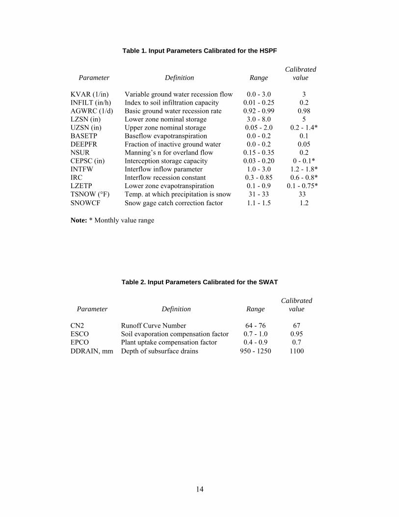
Definition of various HSPF model parameters calibrated in this study is given in Table 1.

These parameters and the respective ranges within which their values were varied were selected

based on other evaluation studies using HSPF (Duncker et al., 1995; Jones and Winterstein

(2000), Laroche et al. (1996), Chew et al. (1991), Bergman and Donnangelo (2000), and the

BASINS Technical Note-6 (USEPA, 2000). The model was run on an hourly time step and

output was obtained on daily basis. A stepwise approach was used for HSPF calibration in which

first an acceptable match was obtained between annual and monthly streamflows. Model

parameters were then further adjusted to obtain a satisfactory agreement between observed and

simulated streamflow hydrographs and daily flow-duration curves. This approach was supported

by the hierarchical structure in HSPF in which annual streamflow values are affected by one set

7

of parameters (e.g. LZETP, DEEPFR, LZSN, and INFILT parameters), monthly flows by

another set (UZSN, BASETP, KVARY, AGWRC, and CEPSC), and storm flows by a third set

(e.g. INFILT, INTFW, and IRC). Snowmelt and freezing phenomena in the watershed were

simulated by changing the values of SNOWCF, TSNOW, and CCFACT parameters associated

with the snow simulation component of the HSPF.

SWAT was also calibrated using a similar stepwise procedure as followed for the HSPF.

Model parameters to be calibrated and ranges within which their values were varied (Table 2)

were selected based on calibration guidelines provided in Neithch et al. (2002), Arnold et al.

(2000), Santhi et al. (2001). SWAT runs on daily time step and output was also generated on

daily basis. Estimates of values of all the four parameters (Table 2) were obtained during initial

model calibration runs which focused on fitting the long term, annual, and monthly streamflows.

Fine tuning of only most sensitive parameters – CN2 and ESCO, was done further so as to obtain

a reasonable match between streamflow hydrographs and flow-duration curves. Surface runoff is

extremely sensitive to parameter CN2. Decreasing the CN2 values results in decreasing runoff,

and increasing infiltration, base flow and recharge. Parameters ESCO and EPCO were varied to

adjust depth distribution for evaporation and plant uptake of water, respectively, from the soil

profile. Depth of subsurface drains was adjusted between 950 to 1250mm. Values of other two

parameters that affect time to drain the soil profile, and time till water enters the channel network

after entering the tiles were set to 24h and 48h, respectively.

Results and Discussion HSPF Calibration

During the nine year calibration period (1987-1995) the absolute value of the volume

error between observed and HSPF simulated annual streamflows was less than 10% (very good

simulation) in three years and 10-15% (good simulation) in four years (Table 3). Out of the nine

years, HSPF oversimulated (2.6% to 49.5%) the streamflow in seven and undersimulated (-0.2

and -13.8%) it in two years. Model oversimulated streamflow in 1988 by 49.5% which was a dry

year that had received 31% less precipitation than the average. The average observed

streamflows, and HSPF simulated streamflows and actual ET during calibration period were

37%, 38%, and 59% of the total precipitation received by the IRW during that period.

8

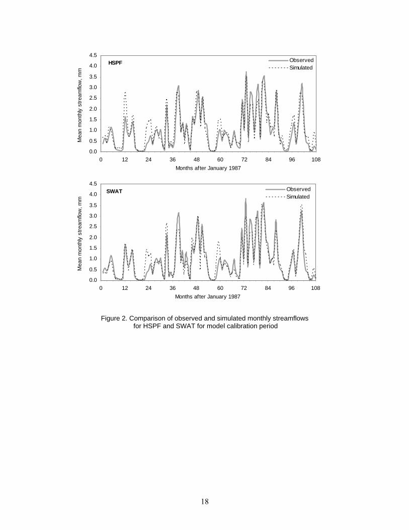
Model predicted mean monthly streamflows satisfactorily as indicated by NSE = 0.88

and r = 0.94 (Table 4). Visual comparison of observed and HSPF simulated mean monthly

hydrographs (Figure 2) also shows this satisfactory agreement. Out of 108 months in calibration

period, the absolute volume error between observed and simulated mean monthly values were

less than 10% in 24 months, 10-15% in 11 months, and 15-25% in 13 months, as shown in Table

4.

Statistics resulting from comparison of daily observe and simulated streamflows for the

calibration period for the two models are given in Table 5. HSPF simulated and observed

streamflow values and their SD were close with a mean volume error of only 4.7% (very good

fit) over the nine year period. Low RMSE (= 0.57mm) and MAE (= 0.33mm), and high NSE (=

0.81) and r (= 0.90) values for daily flow comparisons suggest that the model was well calibrated

to simulate daily streamflows satisfactorily. Also, flow-duration curves for observed and

simulated daily streamflows closely match for the most part (Figure 3). Only some low flows in

the exceedance range of 75-95% were oversimulated by the model. Overall, the calibrated model

simulated the range in magnitude of daily streamflows reasonably well. Comparison of daily

observed and HSPF simulated streamflow time-series for a four year period from 01/01/1992 to

12/31/1995 is shown in Figure 7. Despite high variability of annual precipitation during this

period (49% above average in 1993, 10% and 13% below average in 1992 and 1994, and near

average precipitation in 1995) shape and timing of the observed and simulated streamflow

hydrographs agree for most part of this period. This agreement is evidenced in high values of

daily NSE (=0.83) and r (= 0.91) obtained during this four year period (Figure 4).

SWAT Calibration

The absolute value of the volume error between SWAT simulated and observed annual

streamflows was less than 10% for 4 years, 10-15% for 3 years, and 15-25% for one year (Table

3). Out of the nine years, SWAT oversimulated (6.8% to 35.0%) the streamflow in three and

undersimulated (-0.4 to -24.2%) it in six years. Like HSPF, SWAT also oversimulated the flow

during the dry year of 1988, but by a smaller difference of 35%. Thus, average annual

streamflows were slightly better simulated with SWAT than with the HSPF. SWAT simulated

streamflow and actual ET during calibration period as 35% and 63% of the total rainfall that

occurred during that period.

9

For the mean monthly streamflow comparison for SWAT the NSE and r values were 0.89

and 0.94 (Table 4), indicating satisfactory calibration of the model. This agreement between

observed and HSPF simulated mean monthly hydrographs is also evidenced in Figure 2. Like

HSPF, the absolute volume error between observed and SWAT simulated mean monthly flows

were less than 10% for 24 months, and 10-15% for 11 months. However, in case of SWAT the

number of months with volume error 15-25% (= 32) was more than two times the number of

months with volume error in this range during HSPF simulations.

For SWAT also mean observed and simulated daily flows and their SD matched well

during calibration period and model undersimulated the streamflows by 4.7% indicating ‘very

good’ fit during this nine year period. The low daily RMSE (= 0.60mm) and MAE (= 0.35mm)

values, and high daily NSE (= 0.79) and r (= 0.90) values for SWAT simulations (Table 5) over

this period suggest that the model was well calibrated to simulate daily streamflows. Observed

and SWAT simulated daily flow-duration curves also matched well (Figure 3) except that model

undersimulated some very low flows in the exceedance range of 90-100%. Comparison of

observed and simulated daily streamflow time-series for 01/01/1992 to 12/31/1995 (Figure 4)

showed that shape and timings of the observed and simulated hydrographs agree for most part of

the four year period. High daily NSE (=0.84) and r (= 0.92) values obtained during this four year

period (Figure 4) indicated that model was calibrated satisfactorily to simulate daily streamflows

adequately despite extreme variations in the annual precipitation amount during this period, as

explained earlier.

Comparative Performance of HSPF and SWAT during Model Verification Period

During model verification period of 1972-1986, absolute volume error between observed

and HSPF simulated average annual streamflows were less than 10% for ten years, 10-15% for

one year, and 15-25% for two years, respectively (Figure 5). The absolute volume errors for

SWAT simulations during this period were less than 10% for seven years, and 10-15% for five

years as shown in Figure 5. In genreal, both models mostly oversimulated the annual streamflow

during fifteen year verification period. HSPF oversimulated (1.5% to 35.3%) streamflow during

eleven years and undersimulated (-4.5 to -16.9%) it during four years. Likewise, SWAT

oversimulated (0.6% to 33.2%) streamflow during ten years and undersimulated (-0.7 to -26.4%)

it during five years. These statistics indicate that calibrated HSPF and SWAT models can

10

simulate the average annual flows satisfactorily for period outside the calibration period.

However, HSPF performance was slightly better than SWAT when compared based on the

number of years for which the absolute volume error was less than 10%.

Various model performance evaluation statistics for simulating mean monthly

streamflows during verification period were determined and are presented in Table 4 for both the

models. For HSPF, the mean monthly NSE (= 0.82) and r (= 0.91) values suggest that calibrated

HSPF simulated mean monthly streamflows satisfactorily during verification period also. This

agreement between observed and HSPF simulated mean monthly hydrographs for the

verification period is also shown in Figure 6. Absolute volume error for HSPF simulated mean

monthly flows were less than 10% for twenty eight months, 10-15% for eleven months, and 15-

25% for thirty two months. For SWAT simulations during verification period, slightly smaller

RMSE (=0.38mm) but same MAE (= 0.28mm) were obtained compared to HSPF simulations.

Also, the NSE (= 0.83) and r (= 0.92) values obtained for SWAT simulations were marginally

better than those obtained for the HSPF (Table 4). Observed and SWAT simulated mean

monthly hydrographs, as shown in Figure 6 for the verification period, also show close

agreement between the two. For SWAT simulated mean monthly flows, the absolute volume

errors were less than 10% for thirty three months, 10-15% for nineteen months, and 15-25% for

twenty eight months, respectively (Table 4). Though both models simulated mean monthly

streamflows satisfactorily during verification period, overall performance of SWAT was slightly

superior than that of the HSPF as shown by marginally better statistics.

Model performance evaluation statistics for simulating daily flows during verification

period are given in Table 5 for both HSPF and SWAT. Observed and HSPF simulated mean

daily flow values and their SD were very close and model oversimulated streamflow by only

5.3% (very good fit) for this fifteen year period. As shown in Figure 7, flow-duration curves of

observed and simulated daily flows matched well for the most part except for some low flows

which were oversimulated by the model. Low daily RMSE and MAE values of 0.73mm and

0.39mm, and high daily NSE and r values of 0.70 and 0.84 (Table 5) for the HSPF simulations

indicate that the model simulations of daily streamflows during the verification period were

satisfactory. Comparison of observed and HSPF simulated daily streamflow time-series for

01/01/1978 to 12/31/1981 is illustrated in Figure 8 along with various model performance

statistics. Precipitation was highly variable during this period with 19% and 14% below average

11

precipitation in 1978 and 1980, near average in 1979, and 5% above average precipitation in

1981. Some discrepancies can be seen between high as well as low observed and simulated

streamflows. However, the daily NSE = 0.69 and r = 0.83 values obtained for this period indicate

that overall model performance was satisfactory in simulating streamflow hydrographs for this

four period with highly variable annual precipitation values.

SWAT, like HSPF, also oversimulated streamflow during the 1972-1986 model

verification period but by a smaller error of 3.2% only (Table 5) which indicated ‘very good’ fit

for this period. Performance of SWAT in simulating daily streamflows outside the calibration

period was slightly better than the HSPF as indicated by marginally better values of RMSE (=

0.69 mm), MAE (= 0.36mm), NSE (= 0.73), and r (= 0.88) obtained for model verification

(Table 5) This is despite better calibration of the HSPF as indicated by slightly better values of

RMSE, MAE, and NSE for HSPF calibration (Table 5). For most part, close agreement between

SWAT simulated and observed daily streamflow-duration curves was obtained (Figure 7). Only

some very low flows in the exceedance range of 90-100% were undersimulated. Visual

comparison of flow-duration curves for both HSPF and SWAT (Figure 7) also confirmed better

overall performance of SWAT. Observed and SWAT simulated daily streamflow time-series

comparison and resulting statistics are presented in Figure 8 for the four year period from

01/01/1978 to 12/31/1981. Though, like HSPF, results for SWAT also show discrepancies

between some hydrograph peaks as well as low flows, overall performance of SWAT for this

period was better as evidenced in relatively higher NSE (= 0.79) and r (= 0.90) values (Figure 8).

In both HSPF and SWAT poor simulation of low flows could be due to inadequate model

representation of sub-surface storage and subsequent release of water from that storage as

baseflow for large watershed area. In HSPF parameters LZSN and INFILT control the amount of

water in ground water storage component, and parameter AGWRC governs the rate of release of

baseflow from this storage. Model allows only one value each of these parameters for an HRU

for the entire year resulting in inadequate spatio-temporal representation in this study to account

for effects of land use management and heterogeneity in soil physical properties on water storage

in and release from ground water component. In this study HRUs were created based on

dominant landuse (95% agriculture) and soil types (hydrologic soil group B). Also, tile drainage,

which is mostly practiced on flat and poorly drained soils in the IRW is not modeled by HSPF,

may have also resulted in poor simulation of low flows. The water removal effect from the field

12

due to tiling is estimated in HSPF only by adjusting parameters such as INFILT, UZSN, and

LZSN. In SWAT simulation of low flows may be improved to some extent by calibrating the

baseflow recession and groundwater delay parameters. However, simplifications that exist in the

model that describe subsurface flow and channel transmission losses may also be the cause of

discrepancies between observed and simulated flows.

References

Arnold, J.G., R. Srinivasan, R.S. Muttiah, and J.R. Williams, 1998. Large area hydrologic modeling and assessment part I : Model development. J. American Water Resour. Assoc. 34(1): 73-89.

Arnold, J. G., R. S. Muttiah, R. Srinivasan, and P. M. Allen, 2000. Regional estimation of base flow and groundwater recharge in the Upper Mississippi river basin. J. Hydrology, 227: 21-40.

Bergman, M. J., and L. J. Donnangelo, 2000. Simulation of freshwater discharges from ungaged areas to the Sebastian river, Florida. J. American Water Resour. Assoc. 36(5): 1121-1132.

Bicknell, B.R., J.C. Imhoff, J.L. Kittle, Jr., T.H. Jobes, and A.S. Donigian, Jr., 2001. Hydrologic Simulation Program – FORTRAN (HSPF), user’s manual for version 12.0 : USEPA, Athens, GA, 30605.

Chew, C. Y., Moore, L. W., and R. H. Smith, 1991. Hydrologic simulation of Tennessee’s North Reelfoot Creek Watershed. Res. J. Water Pollution Control Federation, v.63: 10-16.

Donigian, A. S., J. C. Imhoff, and B. R. Bicknell, 1983. Predicting water quality resulting from agricultural nonpoint source pollution via simulation – HSPF. In ‘Agricultural management and water quality’, F. W. Schaller and G.W. Bailey, eds., Iowa State University Press, Ames, Iowa, 200-249.

Duncker, J.J., Vail, T.J., and C.S. Melching, 1995. Regional rainfall-runoff relations for simulation of streamflow for watersheds in Lake County, Illinois, USGS WRIR 95-4023.

Jones, P.M. and T.A. Winterstein, 2000. Characterization of rainfall-runoff response and estimation of the effect of wetland restoration on runoff, Herone Lake Basin, southwestern Minnesota, 1991-97. USGS WRI Report 00-4095.

Knapp, H. V. 1992. Kankakee River basin streamflow assessment model: Hydrologic analysis. Illinois State Water Survey contract report 541, Champaign, IL.

Laroche, A-M., J. Gallichand, R. Lagace, and A Pesant, 1996: Simulating Atrazine Transport with HSPF in an Agricultural Watershed. J. Environmental Eng., 122(7):622.

13

Nash, J.E. and Sutcliffe, J.V. (1970). River flow forecasting through conceptual models, Part 1 – a discussion of principles. J. Hydrology, 10(3), 282-290.

Neitsch, S. L., J. G. Arnold, J. R. Kiniry, R. Srinivasan, and J. R. Williams, 2002. Soil and Water Assessment Tool User’s Manual: Version 2000. GSWRL Report 02-02, BRC Report 02-06, Publ. Texas Water Resources Institute, TR-192, College Station, Texas, 438 pp.

Santhi, C., J. G. Arnold, J. R. Williams, W. A. Dugas, R. Srinivasan, and L. M. Hauck. 2001. Validation of the SWAT model on a large river basin with point and nonpoint sources. J. American Water Resour. Assoc. 37(5): 1169-1188.

USEPA, 2001. Better Assessment Science Integrating Point and Nonpoint Sources -BASINS version 3.0, User's Manual. EPA-823-B-01-001.

USEPA. 2000. BASINS Technical Note 6: Estimating Hydrology and Hydraulic Parameters for HSPF. USEPA, Office of Water. EPA-823-R-99-013.

14

Table 1. Input Parameters Calibrated for the HSPF

Parameter Definition Range Calibrated

value KVAR (1/in) Variable ground water recession flow 0.0 - 3.0 3 INFILT (in/h) Index to soil infiltration capacity 0.01 - 0.25 0.2 AGWRC (1/d) Basic ground water recession rate 0.92 - 0.99 0.98 LZSN (in) Lower zone nominal storage 3.0 - 8.0 5 UZSN (in) Upper zone nominal storage 0.05 - 2.0 0.2 - 1.4* BASETP Baseflow evapotranspiration 0.0 - 0.2 0.1 DEEPFR Fraction of inactive ground water 0.0 - 0.2 0.05 NSUR Manning’s n for overland flow 0.15 - 0.35 0.2 CEPSC (in) Interception storage capacity 0.03 - 0.20 0 - 0.1* INTFW Interflow inflow parameter 1.0 - 3.0 1.2 - 1.8* IRC Interflow recession constant 0.3 - 0.85 0.6 - 0.8* LZETP Lower zone evapotranspiration 0.1 - 0.9 0.1 - 0.75* TSNOW (°F) Temp. at which precipitation is snow 31 - 33 33 SNOWCF Snow gage catch correction factor 1.1 - 1.5 1.2

Note: * Monthly value range

Table 2. Input Parameters Calibrated for the SWAT

Parameter Definition Range Calibrated

value CN2 Runoff Curve Number 64 - 76 67 ESCO Soil evaporation compensation factor 0.7 - 1.0 0.95 EPCO Plant uptake compensation factor 0.4 - 0.9 0.7 DDRAIN, mm Depth of subsurface drains 950 - 1250 1100

15

Table 3. Observed Precipitation and Streamflow, and HSPF and SWAT Simulated Actual Evapotranspiration, Streamflow, and Percent Error for Calibration Period

Year 1987 1988 1989 1990 1991 1992 1993 1994 1995 Precipitation, mm 850 684 863 1230 794 903 1472 858 987 Obs-Q, mm 192 159 245 490 363 272 832 284 330 HSPF: Actual ET, mm 593 427 552 612 502 564 631 591 618 Sim-Q, mm 248 238 278 503 356 278 717 319 371

Error,% 29.1 49.5 13.4 2.6 -2.0 2.3 -

13.8 12.5 12.4 SWAT: Actual ET, mm 648 459 625 667 517 654 684 615 608 Sim-Q, mm 156 215 262 422 362 206 764 264 369

Error,% -

18.8 35.0 6.8 -

14.0 -0.4 -

24.2 -8.1 -6.9 11.8 Note: Obs-Q = Observed streamflow, Sim-Q = Simulated streamflow

Table 4. Model Calibration and Verification Statistics for HSPF and SWAT for Monthly Streamflow Comparison

Calibration Period Verification Period

(1987-1995) (1972-1986) HSPF SWAT HSPF SWAT NSE 0.88 0.89 0.82 0.83 r 0.94 0.94 0.91 0.92 RMSE, mm 0.33 0.31 0.39 0.38 MAE, mm 0.23 0.21 0.28 0.26 Number of months with volume error:

<10% 24 24 28 33 10-15% 11 11 11 19 15-25% 13 32 32 28

16

Table 5. Model Calibration and Verification Statistics for HSPF and SWAT for Daily Streamflow Comparison

Calibration Period Verification Period (1987-1995) (1972-1986) HSPF SWAT HSPF SWAT Observed mean (SD), mm 0.96(1.31) 0.96(1.31) 0.95(1.33) 0.95(1.33)Simulated mean (SD), mm 1.01(1.26) 0.92(1.35) 1.00(1.22) 0.98(1.41)Mean volume error, % 4.70 -4.71 5.26 3.20 NSE 0.81 0.79 0.70 0.73 r 0.90 0.90 0.84 0.88 RMSE, mm 0.57 0.60 0.73 0.69 MAE, mm 0.33 0.35 0.39 0.36

17

#*

Figure 1. Iroquois River watershed and location of precipitation and streamflow gaging stations

Rensselaer

Kentland

Watseka Piper City

Kankakee Sewage Plant

Hoopeston

USGS 05526000 near Chebanse, IL

Lake Michigan

IND

IAN

A

ILLI

NO

IS

N

Precipitation Gage

Streamflow Gage

IL IN

18

HSPF

0.0

0.5

1.0

1.5

2.0

2.5

3.0

3.5

4.0

4.5

0 12 24 36 48 60 72 84 96 108Months after January 1987

Mea

n m

onth

ly s

tream

flow

, mm

ObservedSimulated

SWAT

0.0

0.5

1.0

1.5

2.0

2.5

3.0

3.5

4.0

4.5

0 12 24 36 48 60 72 84 96 108Months after January 1987

Mea

n m

onth

ly s

tream

flow

, mm

ObservedSimulated

Figure 2. Comparison of observed and simulated monthly streamflows for HSPF and SWAT for model calibration period

19

HSPF

0.001

0.01

0.1

1

10

100

0 20 40 60 80 100% time streamflow is equalled or exceeded

Dai

ly s

tream

flow

, mm

ObservedSimulated

SWAT

0.001

0.01

0.1

1

10

100

0 20 40 60 80 100% time streamflow is equalled or exceeded

Dai

ly S

tream

flow

, mm

Observed

Simulated

Figure 3. Comparison of observed and simulated daily streamflow-duration curves for the model calibration period

20

HSPF

0.0

2.0

4.0

6.0

8.0

10.0

12.0

0 120 240 360 480 600 720 840 960 1080 1200 1320 1440

Days after 01/01/1992

Dai

ly s

tream

flow

, mm

Observed

Simulated

SWAT

0.0

2.0

4.0

6.0

8.0

10.0

12.0

0 120 240 360 480 600 720 840 960 1080 1200 1320 1440

Days after 01/01/1992

Dai

ly s

tream

flow

, mm

Observed

Simulated

Figure 4. Comparison of observed and simulated daily streamflow time-seris

for HSPF and SWAT for 1992-1995

NSE = 0.83 r = 0.91

NSE = 0.84 r = 0.92

21

HSPF

0.0

0.2

0.4

0.6

0.8

1.0

1.2

1.4

1.6

1972 1973 1974 1975 1976 1977 1978 1979 1980 1981 1982 1983 1984 1985 1986Year

Mea

n an

nual

stre

amflo

w, m

m

Observed SimulatedS i 4

SWAT

0.0

0.2

0.4

0.6

0.8

1.0

1.2

1.4

1.6

1972 1973 1974 1975 1976 1977 1978 1979 1980 1981 1982 1983 1984 1985 1986Year

Mea

n an

nual

stre

amflo

w, m

m

Observed SimulatedS i 4

Figure 5. Comparison of observed and simulated annual streamflows and their percent errors for HSPF and SWAT for model verification period of 1972-1986

22

HSPF

0.0

1.0

2.0

3.0

4.0

5.0

6.0

0 12 24 36 48 60 72 84 96 108 120 132 144 156 168 180Months after January 1972

Mea

n m

onth

ly s

tream

flow

, mm

Observed

Simulated

SWAT

0.0

1.0

2.0

3.0

4.0

5.0

6.0

0 12 24 36 48 60 72 84 96 108 120 132 144 156 168 180Months after January 1972

Mea

n m

onth

ly s

tream

flow

, mm

Observed

Simulated

Figure 6. Comparison of observed and simulated monthly streamflows for HSPF and SWAT for model verification period of 1972-1986

23

HSPF

0.001

0.01

0.1

1

10

100

0 20 40 60 80 100

% time streamflow is equalled or exceeded

Dai

ly S

tream

flow

, mm

Observed

Simulated

SWAT

0.001

0.01

0.1

1

10

100

0 20 40 60 80 100% time streamflow is equalled or exceeded

Dai

ly S

tream

flow

, mm

Observed

Simulated

Figure 7. Comparison of observed and simulated daily streamflow-duration curves for the model verification period

24

HSPF

0.0

2.0

4.0

6.0

8.0

10.0

12.0

14.0

0 120 240 360 480 600 720 840 960 1080 1200 1320 1440

Days after 01/01/1978

Dai

ly s

tream

flow

, mm

ObservedSimulated

SWAT

0.0

2.0

4.0

6.0

8.0

10.0

12.0

14.0

0 120 240 360 480 600 720 840 960 1080 1200 1320 1440Days after 01/01/1978

Dai

ly s

tream

flow

, mm

ObservedSimulated

Figure 8. Comparison of observed and simulated daily streamflow time-series for HSPF and SWAT for 1978-1981

NSE = 0.69 r = 0.83

NSE = 0.79 r = 0.90