Embed Size (px)
Citation preview

Hydrology and Watershed Analysis
Manual By: Elyse Maurer
Reference Map
Figure 1. This map provides context to the area of Washington State that is being focused on.
The red outline indicates the boundary of our basin.
Re-projection
From NAD 1927 UTM Zone 10 N to NAD 1983 Zone 10 N
*Note: Do not re-project the DEM file until it is properly clipped to your boundary. This will
greatly reduce processing time.
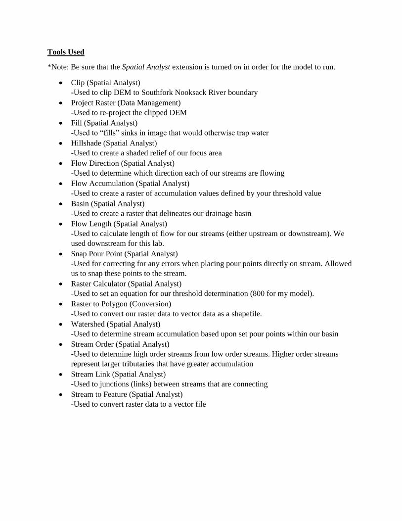
Tools Used
*Note: Be sure that the Spatial Analyst extension is turned on in order for the model to run.
Clip (Spatial Analyst)
-Used to clip DEM to Southfork Nooksack River boundary
Project Raster (Data Management)
-Used to re-project the clipped DEM
Fill (Spatial Analyst)
-Used to “fills” sinks in image that would otherwise trap water
Hillshade (Spatial Analyst)
-Used to create a shaded relief of our focus area
Flow Direction (Spatial Analyst)
-Used to determine which direction each of our streams are flowing
Flow Accumulation (Spatial Analyst)
-Used to create a raster of accumulation values defined by your threshold value
Basin (Spatial Analyst)
-Used to create a raster that delineates our drainage basin
Flow Length (Spatial Analyst)
-Used to calculate length of flow for our streams (either upstream or downstream). We
used downstream for this lab.
Snap Pour Point (Spatial Analyst)
-Used for correcting for any errors when placing pour points directly on stream. Allowed
us to snap these points to the stream.
Raster Calculator (Spatial Analyst)
-Used to set an equation for our threshold determination (800 for my model).
Raster to Polygon (Conversion)
-Used to convert our raster data to vector data as a shapefile.
Watershed (Spatial Analyst)
-Used to determine stream accumulation based upon set pour points within our basin
Stream Order (Spatial Analyst)
-Used to determine high order streams from low order streams. Higher order streams
represent larger tributaries that have greater accumulation
Stream Link (Spatial Analyst)
-Used to junctions (links) between streams that are connecting
Stream to Feature (Spatial Analyst)
-Used to convert raster data to a vector file
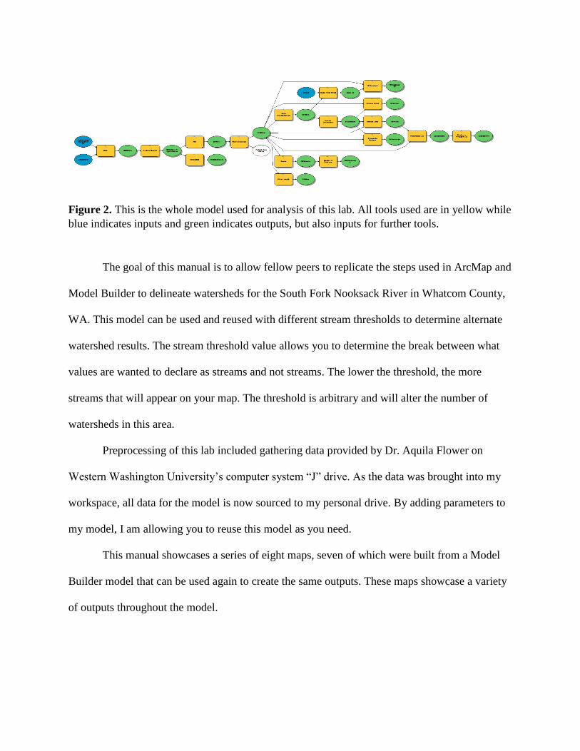
Figure 2. This is the whole model used for analysis of this lab. All tools used are in yellow while
blue indicates inputs and green indicates outputs, but also inputs for further tools.
The goal of this manual is to allow fellow peers to replicate the steps used in ArcMap and
Model Builder to delineate watersheds for the South Fork Nooksack River in Whatcom County,
WA. This model can be used and reused with different stream thresholds to determine alternate
watershed results. The stream threshold value allows you to determine the break between what
values are wanted to declare as streams and not streams. The lower the threshold, the more
streams that will appear on your map. The threshold is arbitrary and will alter the number of
watersheds in this area.
Preprocessing of this lab included gathering data provided by Dr. Aquila Flower on
Western Washington University’s computer system “J” drive. As the data was brought into my
workspace, all data for the model is now sourced to my personal drive. By adding parameters to
my model, I am allowing you to reuse this model as you need.
This manual showcases a series of eight maps, seven of which were built from a Model
Builder model that can be used again to create the same outputs. These maps showcase a variety
of outputs throughout the model.
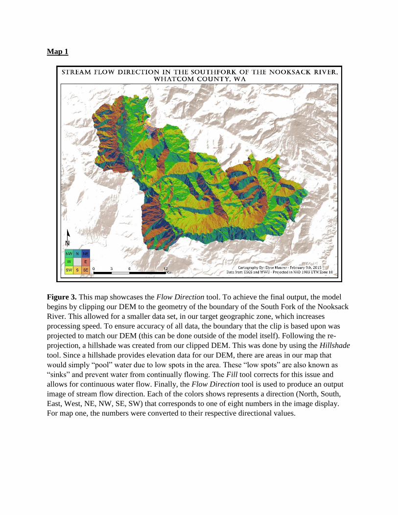
Map 1
Figure 3. This map showcases the Flow Direction tool. To achieve the final output, the model
begins by clipping our DEM to the geometry of the boundary of the South Fork of the Nooksack
River. This allowed for a smaller data set, in our target geographic zone, which increases
processing speed. To ensure accuracy of all data, the boundary that the clip is based upon was
projected to match our DEM (this can be done outside of the model itself). Following the re-
projection, a hillshade was created from our clipped DEM. This was done by using the Hillshade
tool. Since a hillshade provides elevation data for our DEM, there are areas in our map that
would simply “pool” water due to low spots in the area. These “low spots” are also known as
“sinks” and prevent water from continually flowing. The Fill tool corrects for this issue and
allows for continuous water flow. Finally, the Flow Direction tool is used to produce an output
image of stream flow direction. Each of the colors shows represents a direction (North, South,
East, West, NE, NW, SE, SW) that corresponds to one of eight numbers in the image display.
For map one, the numbers were converted to their respective directional values.
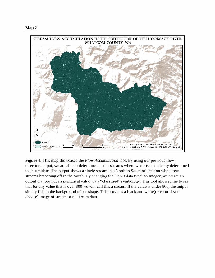
Map 2
Figure 4. This map showcased the Flow Accumulation tool. By using our previous flow
direction output, we are able to determine a set of streams where water is statistically determined
to accumulate. The output shows a single stream in a North to South orientation with a few
streams branching off in the South. By changing the “input data type” to Integer, we create an
output that provides a numerical value via a “classified” symbology. This tool allowed me to say
that for any value that is over 800 we will call this a stream. If the value is under 800, the output
simply fills in the background of our shape. This provides a black and white(or color if you
choose) image of stream or no stream data.
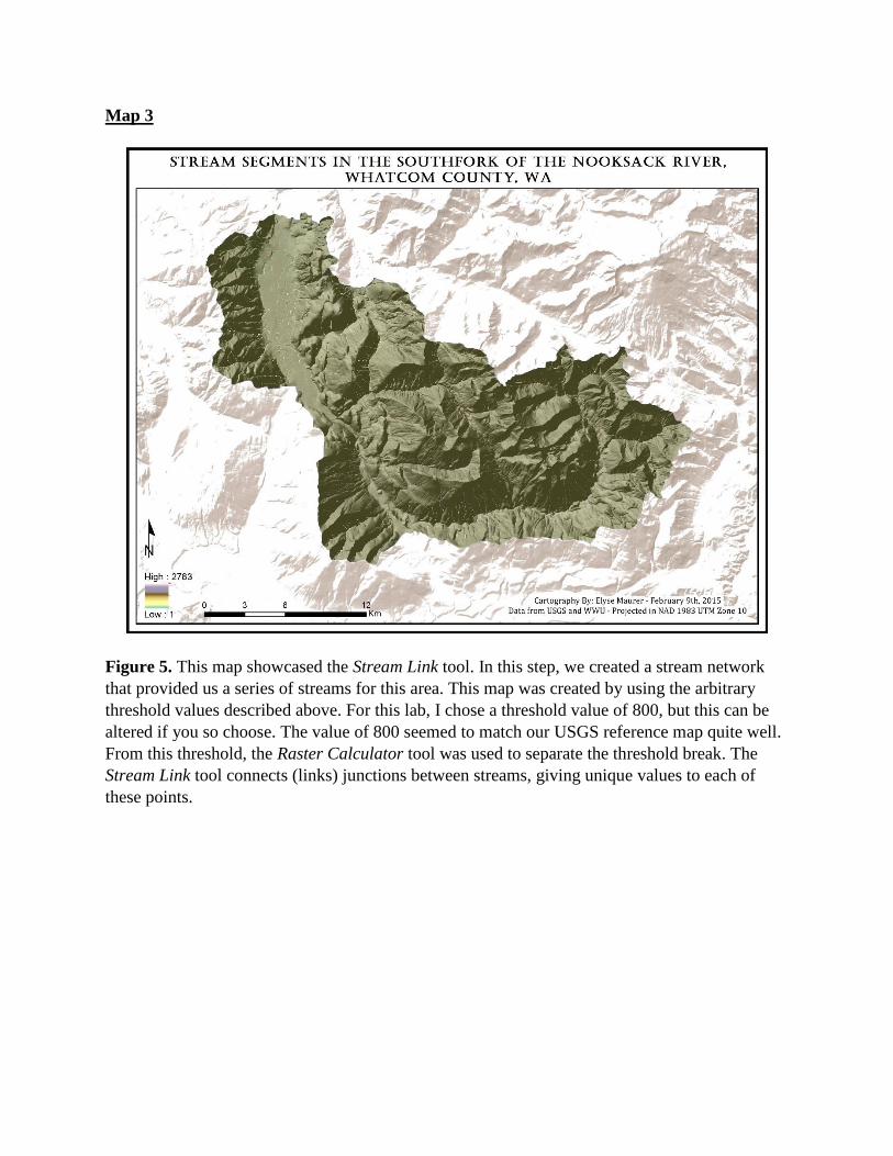
Map 3
Figure 5. This map showcased the Stream Link tool. In this step, we created a stream network
that provided us a series of streams for this area. This map was created by using the arbitrary
threshold values described above. For this lab, I chose a threshold value of 800, but this can be
altered if you so choose. The value of 800 seemed to match our USGS reference map quite well.
From this threshold, the Raster Calculator tool was used to separate the threshold break. The
Stream Link tool connects (links) junctions between streams, giving unique values to each of
these points.
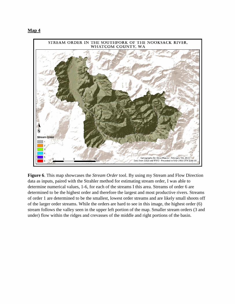
Map 4
Figure 6. This map showcases the Stream Order tool. By using my Stream and Flow Direction
data as inputs, paired with the Strahler method for estimating stream order, I was able to
determine numerical values, 1-6, for each of the streams I this area. Streams of order 6 are
determined to be the highest order and therefore the largest and most productive rivers. Streams
of order 1 are determined to be the smallest, lowest order streams and are likely small shoots off
of the larger order streams. While the orders are hard to see in this image, the highest order (6)
stream follows the valley seen in the upper left portion of the map. Smaller stream orders (3 and
under) flow within the ridges and crevasses of the middle and right portions of the basin.
Map 5:
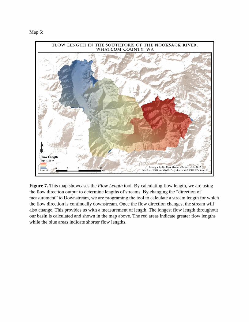
Figure 7. This map showcases the Flow Length tool. By calculating flow length, we are using
the flow direction output to determine lengths of streams. By changing the “direction of
measurement” to Downstream, we are programing the tool to calculate a stream length for which
the flow direction is continually downstream. Once the flow direction changes, the stream will
also change. This provides us with a measurement of length. The longest flow length throughout
our basin is calculated and shown in the map above. The red areas indicate greater flow lengths
while the blue areas indicate shorter flow lengths.
Map 6
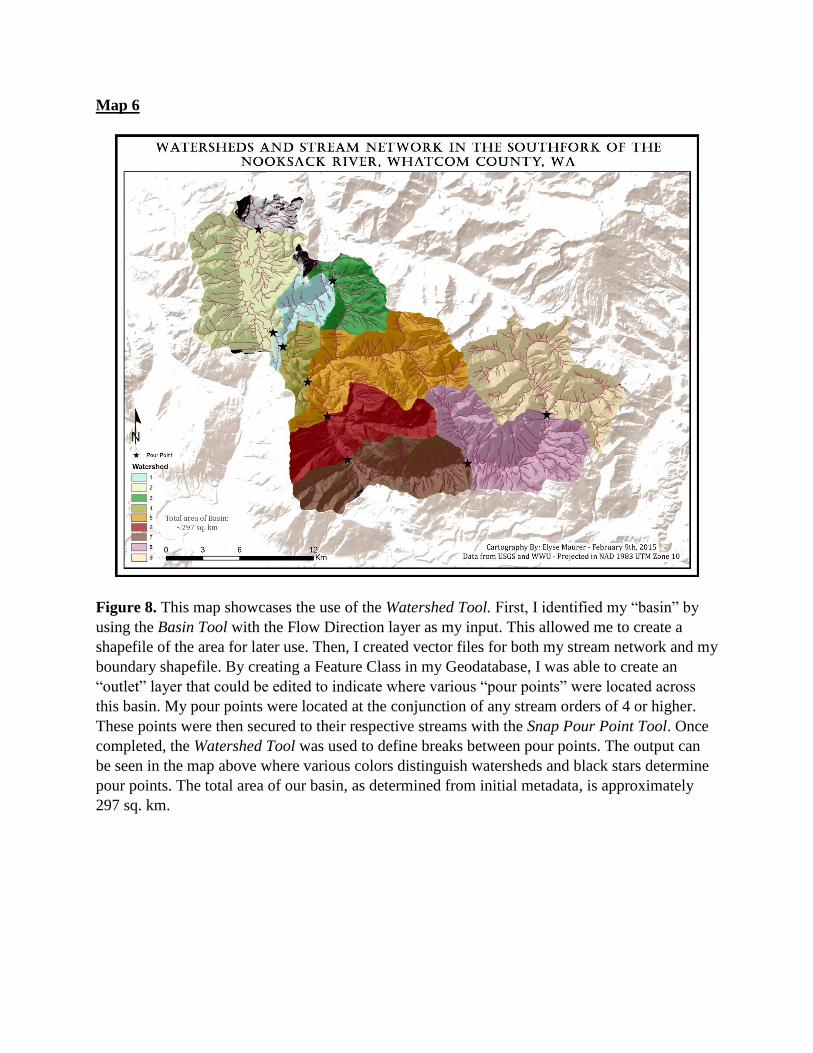
Figure 8. This map showcases the use of the Watershed Tool. First, I identified my “basin” by
using the Basin Tool with the Flow Direction layer as my input. This allowed me to create a
shapefile of the area for later use. Then, I created vector files for both my stream network and my
boundary shapefile. By creating a Feature Class in my Geodatabase, I was able to create an
“outlet” layer that could be edited to indicate where various “pour points” were located across
this basin. My pour points were located at the conjunction of any stream orders of 4 or higher.
These points were then secured to their respective streams with the Snap Pour Point Tool. Once
completed, the Watershed Tool was used to define breaks between pour points. The output can
be seen in the map above where various colors distinguish watersheds and black stars determine
pour points. The total area of our basin, as determined from initial metadata, is approximately
297 sq. km.
Map 7
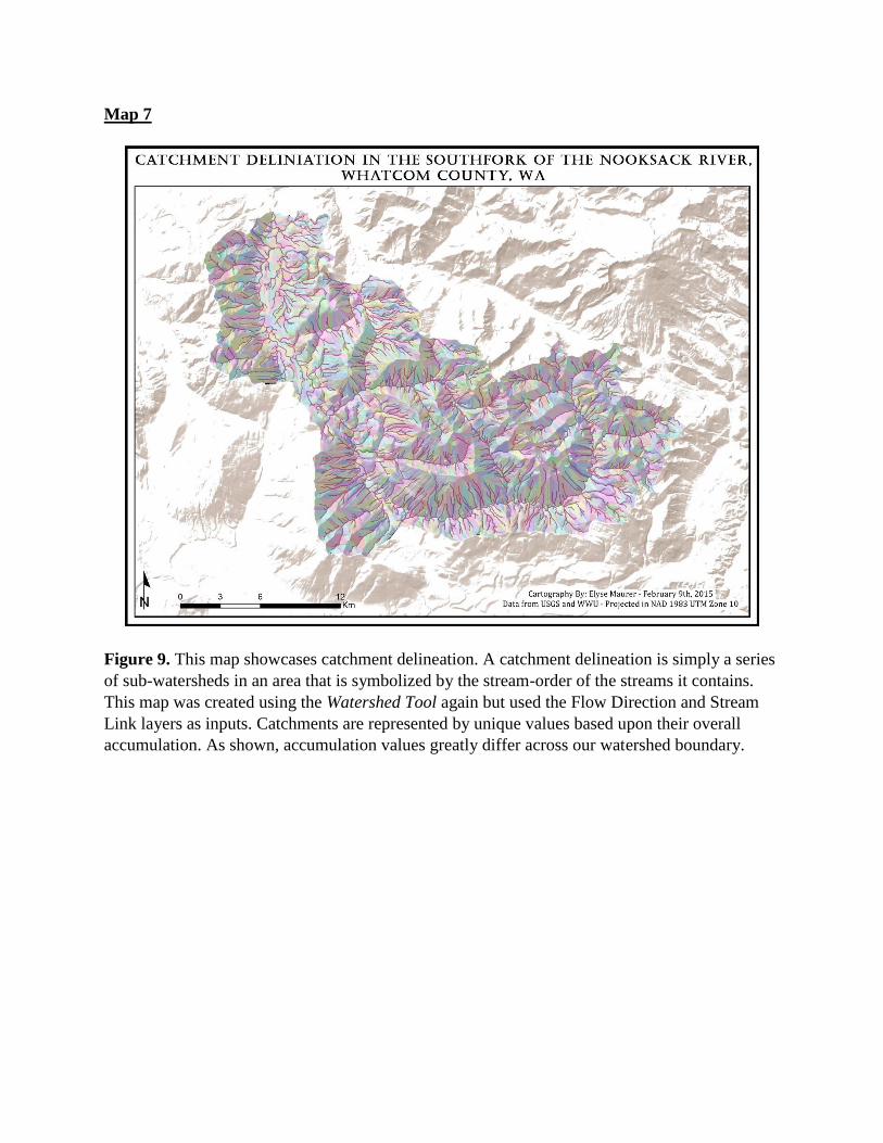
Figure 9. This map showcases catchment delineation. A catchment delineation is simply a series
of sub-watersheds in an area that is symbolized by the stream-order of the streams it contains.
This map was created using the Watershed Tool again but used the Flow Direction and Stream
Link layers as inputs. Catchments are represented by unique values based upon their overall
accumulation. As shown, accumulation values greatly differ across our watershed boundary.
Map 8
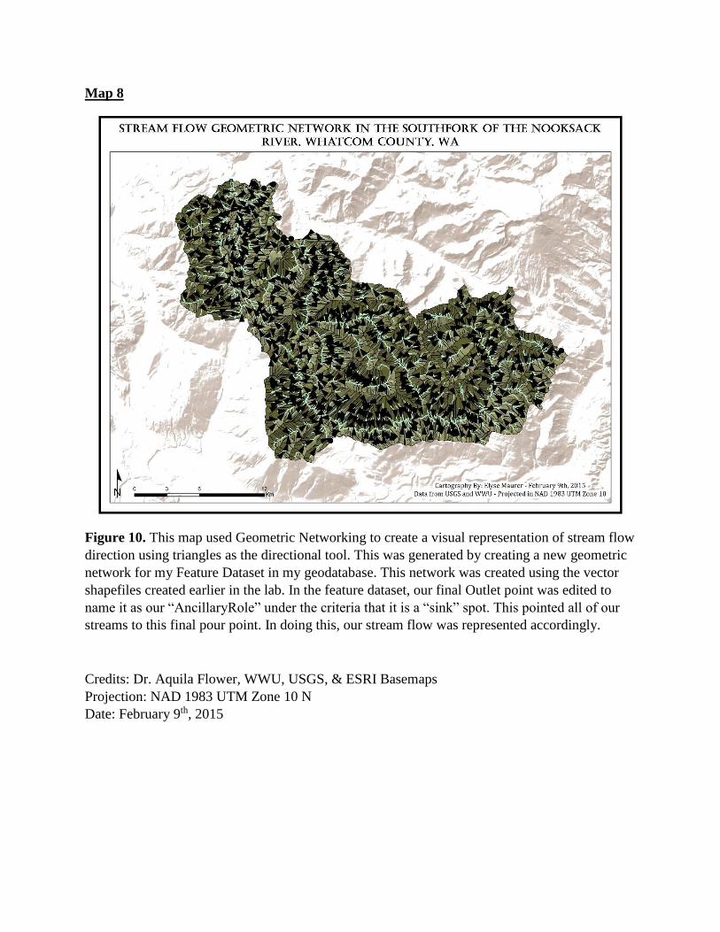
Figure 10. This map used Geometric Networking to create a visual representation of stream flow
direction using triangles as the directional tool. This was generated by creating a new geometric
network for my Feature Dataset in my geodatabase. This network was created using the vector
shapefiles created earlier in the lab. In the feature dataset, our final Outlet point was edited to
name it as our “AncillaryRole” under the criteria that it is a “sink” spot. This pointed all of our
streams to this final pour point. In doing this, our stream flow was represented accordingly.
Credits: Dr. Aquila Flower, WWU, USGS, & ESRI Basemaps
Projection: NAD 1983 UTM Zone 10 N
Date: February 9th, 2015