Hyperacuity Sensing for Image Processingalumni.media.mit.edu/~sbasu/papers/SB_thesis.pdf · development and effectiveness of a scanning system that has a similarly varying ... S.B

1

Hyperacuity Sensing for Image Processing

Sumit [email protected]

Advisors: Warren Jackson (Xerox PARC)David Biegelsen (Xerox PARC) David Jared (Xerox PARC)Fernando Corbató (MIT)

Abstract

The human eye’s response to high spatial frequency content in images is highly depen-dent on the nature of the features: the eye integrates periodic intensity variations at highfrequencies to form a solid gray, yet is very sensitive to high-contrast steps in intensity(which contain high frequency components), such as edges. This study presents thedevelopment and effectiveness of a scanning system that has a similarly varyingresponse to spatial frequency content. The system is implemented by an array of PSD(position sensitive detector) scanning elements, each of which produces four valueswhich can be composed to retrieve intensity and intensity gradient information over thedetector’s area. It is shown that this information, along with additional information fromimmediately neighboring pixels, can be used to determine the frequency content andedge locations of the image area covered by the detector. The accuracy of this determi-nation is shown to vary in a way similar to that of the human eye’s response. A single-pass algorithm (BBJJ) is developed which determines how to render the area of theimage corresponding to each detector as either an edge or a smooth gradient. A versionof the algorithm is also presented for standard scanning detectors, which composes theinformation from multiple detectors to construct values analogous to those availablefrom each PSD element. The algorithms described were implemented in an existingsimulation framework. The performance of each of these methods in comparison to thatof a standard scanning system is shown (in simulation) for three major classes ofimages: line art, continuous tone, and halftoned images.

Perceptual Computing

Sumit Basu. "Hyperacuity Sensing for Image Processing." S.B. Thesis, MIT Department of Electrical Engineering and Computer Science (EECS), 1995.

Introduction

Hyperacuity Sensing for Image Processing 2

Introduction

The typical approach to improving performance in scanning systems has been toincrease the density of the scanning elements. While this undeniably improves theimage quality, it is usually not an efficient or economic solution. Consider , for example,an image that has a single, solid black circle in the center of a white background. A typ-ical scanning system will take the average intensity incident on each detector-sized areaof this image and represent this value in an n by n pixel block on the screen, where n isthe scaling factor. At lower resolutions, this approach results in “jaggies” (jagged linesthat did not exist in the original image - see, for example, Figure 20). Sampling at higherand higher resolutions certainly reduces the visibility of these features, but also resultsin sampling constant-intensity regions at an unnecessarily high resolution.

In this paper, a method is presented for reconstructing image features without going tohigher resolutions by using a novel scanning element, the PSD, and an algorithm whichcomposes the output from these devices and their nearest neighbors to reconstruct sub-detector sized features. An algorithm is also presented for performing this reconstruc-tion using the output from standard grayscale detectors. The goal of this work is not toperfectly rerender an input image - clearly any scanning method will output only a sub-set of the information content of the original, and thus a perfect reconstruction is impos-sible. Instead, the goal is to faithfully reproduce only the visually significant features -those features that are visible to the human eye at a normal viewing distance. In otherwords, the standard of reconstructed image quality to be used is not simply the squaredpixel-by-pixel error between the original and reconstructed images, but one which takesinto account the response of the human visual system. Prior research has suggested con-vincing arguments for adopting such a stance (see Pearlman [11] and Bloomer [1]). Byadopting this standard, it is possible to measure the practical performance of these meth-ods without worrying over features that are effectively invisible to the eye.

The Hyperacuity Model

The inspiration for this work came from the operation of the human visual system.Though the eye has a relatively low “detector density” in terms of light receptors, thevisual system employs various techniques that produce what appear to be very high res-olution images. Though the exact workings of this system are not known, it is possibleto gain some understanding of what goes on from observing the visual response to vari-ous image features. This response varies greatly with the size and quality of the featuresin the image. For a pattern of adjacent vertical strips of 0% and 100% intensities (blackand white, respectively), the ability of the human visual system to distinguish the pat-tern from the average gray drops off significantly at around 300 cycles/inch for a stan-dard viewing distance of 12”. For lower levels of contrast between the intensities, thereponse drops off at even lower spatial frequencies. On the other hand, the visual systemis extremely sensitive to high contrast (non-periodic) steps in an image, such as black-white edges. Though edges contain information at frequencies far higher than 300cycles/inch, the visual system will not blur an edge and is very sensitive to its exactposition. A significant amount of prior research has been performed on this “hyperacu-ity sensing” ability: Nishihara [10] provides a concise description of the effect and citesseveral works examining the effect in detail (citations 1-9). Fahle [2], [3] and Martinez-

Characteristics of the PSD


Uriegas [9] provide explanations and models for the effect. Lennie and D’Zmura [7]examine, for various contrast levels, the transition of the visual system’s response fromdetailed acuity to integrating effects with increasing spatial frequency.

The hyperacuity effect can be easily observed by simply looking at a newspaper pagewith a halftoned image. When held far enough away, the dots in the image will appear toblend into continuous tones, while the edges in the headline text will remain sharp andclear. An ideal scanner should exhibit this effect as well. It should render features withspatial frequencies beyond some range as continuous gray tones, yet be able to place anedge with high pixel accuracy.

The PSD (Position Sensitive Detector) has the capability of achieving this hyperacuitystandard. The four values that the device outputs can be composed to find the centroidof light intensity over the area of the detector and a first-order approximate of the 2Dgradient. As will be shown in later sections, this information can be used to accuratelydetermine sub-detector edge presence and location. Clearly this infomation could not beused to resolve a sequence of twenty black and white strips if it were incident on thedetector - the device would effectively integrate such detail into a solid gray. However,if a single edge were incident on the detector, its position and orientation could be deter-mined exactly (disregarding noise from the device). Thus, in a manner similar to that ofthe human visual system, the PSD integrates periodic high frequency content but is sen-sitive to high-contrast steps in intensity. More specifically, the PSD can be used to accu-rately resolve sub-pixel edges if there is no more than one edge incident on the detector.The development and limitations of this ability will be shown in the following sections.

Characteristics of the PSD

The PSD device itself is basically a simple PIN junction with contacts at each edge heldat virtual ground:

FIGURE 1. The Position Sensitive Detector

When light is incident at a single point on the detector, electron-hole pairs are generatedin the intrinsic layer. The charge pairs separate in the vertical field. The electrons in then-layer then flow to the contacts (all held at ground potential) with currents at each con-

ni

p

incident light

i1 i2

i3

i4

The BBJJ Algorithm


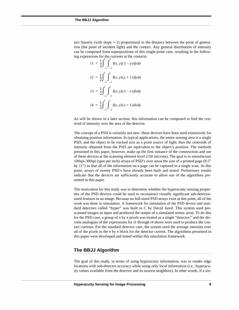
tact linearly (with slope =-1) proportional to the distance between the point of genera-tion (the point of incident light) and the contact. Any general distribution of intensitycan be composed from superpositions of this single-point case, resulting in the follow-ing expressions for the currents at the contacts:

As will be shown in a later section, this information can be composed to find the cen-troid of intensity over the area of the detector.

The concept of a PSD is certainly not new: these devices have been used extensively forobtaining position information. In typical applications, the entire sensing area is a singlePSD, and the object to be tracked acts as a point source of light; thus the centroids ofintensity obtained from the PSD are equivalent to the object’s position. The methodspresented in this paper, however, make up the first instance of the construction and useof these devices at the scanning element level (150 microns). The goal is to manufacture100spi-300spi (spot per inch) arrays of PSD’s over areas the size of a printed page (8.5”by 11”) so that all of the information on a page can be captured in a single scan. At thispoint, arrays of twenty PSD’s have already been built and tested. Preliminary resultsindicate that the devices are sufficiently accurate to allow use of the algorithms pre-sented in this paper.

The motivation for this study was to determine whether the hyperacuity sensing proper-ties of the PSD devices could be used to reconstruct visually significant sub-detector-sized features in an image. Because no full-sized PSD arrays exist at this point, all of thework was done in simulation. A framework for simulation of the PSD device and stan-dard detectors called “hyper” was built in C by David Jared. This system used pre-scanned images as input and produced the output of a simulated sensor array. To do thisfor the PSD case, a group of n by n pixels was treated as a single “detector,” and the dis-crete analogues of the expressions for i1 through i4 above were used to produce the con-tact currents. For the standard detector case, the system used the average intensity overall of the pixels in the n by n block for the detector current. The algorithms presented inthis paper were developed and tested within this simulation framework.

The BBJJ Algorithm

The goal of this study, in terms of using hyperacuity information, was to render edgelocations with sub-detector accuracy while using only local information (i.e., hyperacu-ity values available from the detector and its nearest neighbors). In other words, if a sin-

i112--- I x y,( ) 1 y–( ) y xdd

1–

1

∫1–

1

∫=

i212--- I x y,( ) y 1+( ) y xdd

1–

1

∫1–

1

∫=

i312--- I x y,( ) 1 x–( ) x ydd

1–

1

∫1–

1

∫=

i412--- I x y,( ) x 1+( ) x ydd

1–

1

∫1–

1

∫=

The BBJJ Algorithm


gle black-white edge passed through a detector, the goal was to rerender this edge (andpreserve its location) on the area of the image corresponding to this detector. In contrast,the standard approach in scanning systems is to render the average intensity over thecorresponding area of the image (see Hall [5]).

The algorithm developed in this study to achieve this goal has been named the “BBJJ”algorithm. It models the intensity distribution of a given detector in one of two ways: asa linear edge between two constant intensities or as a non-edge (i.e., a continuous varia-tion in intensity). For the case of an edge, it attempts to determine the location of theedge and the intensity value on each side of the edge, using the values available fromthe detector and its nearest neighbors. For the case of the non-edge, it creates a continu-ous model of the intensity distribution using information from the detector alone.

As opposed to other algorithms which attempt to “segment” an image, i.e., divide it intoregions of various image types and apply different heuristics to each type, the BBJJalgorithm was designed to "autosegment" the image on a detector-by-detector basis.Instead of attempting to determine what areas of the image are grayscale, line art, orhalftone, it applies a constant set of heuristics to every detector. The area correspondingto each detector is thus rendered only on the basis of the information from the detectorand from its nearest neighbors.

The steps of the algorithm are presented in outline form below and then discussed infurther detail in later sections. Note that a separate paper describing the specific meansof implementing the algorithm will be available shortly.

FIGURE 2. Outline of the BBJJ Algorithm

1. Compute I0 (total intensity) and the x and y moments ( and ) of the intensity distibution incident on the detector/macrodetector

2. If the magnitude of the centroid ( ) is large, render area as an edge

a. Find gray value on one side of edge (G1, G2)+If a clear context value exists, use it+Otherwise, use interpolated values

b. Find parametrization of edge from moments using lookup tablesc. Convert gray-on-gray moments to gray-on-black moments

to find actual edge positiond. Use actual edge position to determine other gray valuee. Use edge position and parameters to render area as a

G1, G2 edge3. If the magnitude of the centroid is small, render area as a non-edge

a. Compute the plane/bilinear model parametersb. Render area using plane/bilinear model

Step two, the heart of the BBJJ algorithm, provides the basis for the hyperacuity abili-ties of the detector. The theoretical development of this step will thus be presented first.

x y

x2

y2

+

The BBJJ Algorithm


Afterwards, the particulars of the entire algorithm (all steps) for the PSD (Position Sen-sitive Detector) and standard detector cases will be discussed.

Several basic conventions will be made to simplify the following discussion of the algo-rithm. First, the detector’s area is on a coordinate system as shown below:

FIGURE 3. The detector coordinate system

Second, the intensity function I(x,y) is defined over this area, giving the intensity at eachpoint on the detector. The integral of this function over the area of the detector results inthe total light intensity incident on the detector, I0. Third, a high intensity value (100.0)indicates a white region, while a low intensity (0.0) indicates a black region.

Assumptions

We begin by assuming we know the first moments of intensity ( and ) over the areaof the given detector. The x moment is given by:

and the y moment by:

x

y

1

1

-1

-1

x y

x

xI x y,( ) x ydd1–

1

∫1–

1

∫I x y,( ) x ydd

1–

1

∫1–

1

∫---------------------------------------------=

y

yI x y,( ) x ydd1–

1

∫1–

1

∫I x y,( ) x ydd

1–

1

∫1–

1

∫---------------------------------------------=

The BBJJ Algorithm


We also must know the total intensity incident on the detector, I0:

Lastly, it is assumed that there is no more than one edge incident on a given detector,and that all edges are linear unless otherwise indicated. The implications of this lastassumption will be discussed in later sections.

Initial Estimate of Edge Location

If it were known that the detector covered an area containing a uniform gray area and auniform black area of intensity zero (a grey on black edge), the position of the edgecould determined exactly. This is illustrated in the one-dimensional case below:

FIGURE 4. Gray on Black edge

The moment would fall in the exact center of the region of intensity G2, regardless ofG2’s value, as long as it was non-zero and G1 was zero. In other words, we have

.The edge location for a gray-black edge can be similarly found inthe two-dimensional case. The edge is parametrized by the quantities and . isdefined as the angle, measured from the x axis, which describes the orientation of theedge (i.e., a line passing through theta will be normal to the edge location). Note that is always directed towards the high-intensity region. is defined as the distance to theedge along a line passing through . As a result, is not necessarily positive, as illus-trated in the cases below.

I0 I x y,( ) x ydd1–

1

∫1–

1

∫=

xo 1.0

x

G1=0 G2

edge

inte

nsit

y

x

x0 1 2 1 x–( )–=ρ θ θ

θρ

θ ρ

The BBJJ Algorithm


FIGURE 5. Parametrization of Edge Location with and for Two Edge Locations

A unique mapping can be made between space and ( , ) space. An exact for-mulation for and , while possible, is unwieldy and computationally expensive tosolve. A lookup table was used in the implementations in this study.

Returning to the one-dimensional case above (Figure 4), it is clear that when the valueof G1 is raised to a non-zero value, the moment is shifted towards the G1 region. As aresult, the moments will no longer map to the correct edge location. It is thus necessaryto find what the moments would have been had the distribution been that of a gray-blackedge instead of a gray-gray edge.

Fortunately, it is possible to transform the moments of a gray-gray edge to those of agray-black edge if G1 is known. Consider the intensity distribution below. As shownbelow, this can be seen from two perspectives: a region of intensity G1 and one of inten-sity G2, or a region of intensity 0 and a region of intensity (G2-G1), with a constantintensity G1 added to every point of the detector.

FIGURE 6. Two Representations of a Gray on Gray Edge (offsetting by G1)

From the second perspective, the intensity distribution of the detector is I(x) = I’(x) +G1, where I’(x) is 0 for x<x0 and (G2-G1) for x>x0. is then defined as the moment

ρ θ

x

y

ρθ

edge

x y,( )

x

y

ρ 0<

θ

edge

x y,( )

ρ

ρ 0>Case 1: Case 2:

x y,( ) ρ θρ θ

xo 1.0x

G1

G2

inte

nsity

xo 1.0x

0

G2-G1

inte

nsit

y

0

(1) (2)

0x

xx’

x’

The BBJJ Algorithm

Hyperacuity Sensing for Image Process ing 9

corresponding to the intensity distribution described by I’(x). The calculation for thefirst moment of this distribution is shown below for the two-dimensional detector:

If we now refer to the second term in the numerator as IG1, which corresponds to thetotal intensity of a detector covered entirely by intensity G1, we find the followingexpression for , the moment of the gray-black distribution I’(x,y):

The y moment can be transformed in the same way:

This corresponds to what the moment would have been if G1 had been zero (i.e., if thedistribution had been that of a gray-black edge). Because we can find the location of theedge precisely when given the moments of a gray-black edge (see the explanation ofFigure 4), we can use these transformed moment to precisely determine the location ofthe gray-gray edge.

x


1

∫1–

1

∫I x y,( ) x ydd

1–

1

∫1–

1

∫---------------------------------------------

x I’ x y,( ) G1+[ ] x ydd1–

1

∫1–

1

∫I0

----------------------------------------------------------------

x’ I’ x y,( ) x ydd1–

1

∫1–

1

∫I0

------------------------------------------------= = =

since x’

xI’ x y,( ) x ydd1–

1

∫1–

1

∫I’ x y,( ) x ydd

1–

1

∫1–

1

∫---------------------------------------------- xI’ x y,( ) x ydd

1–

1

∫1–

1

∫⇔ x’ I’ x y,( ) x ydd1–

1

∫1–

1

∫= =

and xG1 x ydd1–

1

∫1–

1

∫ G1 x x ydd1–

1

∫1–

1

∫ 0= =

In addition, we can use the relation

I x y,( ) x ydd1–

1

∫1–

1

∫ I’ x y,( ) G1+[ ] x ydd1–

1

∫1–

1

∫ I’ x y,( ) x ydd1–

1

∫1–

1

∫ G1 x ydd1–

1

∫1–

1

∫+= =

to rewrite the expression for x as:

x x’

I x y,( ) x ydd1–

1

∫1–

1

∫ G1 x ydd1–

1

∫1–

1

∫–

I0-----------------------------------------------------------------------------------

x'

I0 G1 x ydd1–

1

∫1–

1

∫–

I0-------------------------------------------

= =

x’

x’ xI0

I0 IG1–------------------

=

y’ yI0

I0 IG1–------------------

=

The BBJJ Algorithm


In some cases, though, IG1 is not available. The transformation of the moments can thenbe performed using IG2 in place of IG1. I’(x,y) is then defined as being (G1-G2) (which isnegative) for x<x0 and 0 for x>x0, as illustrated below

FIGURE 7. Two Representations of a Gray on Gray Edge (offsetting by G2)

The expressions for calculating the transformed moments are the same as those pre-sented earlier, with IG1 replaced by IG2. These transformed moments correspond to thecentroids of the dark region (the region of intensity G1), as opposed to those of the lightregion (as in the previous cases, as shown in Figure 5). Similarly, the resulting nowpoints in the direction of the dark region, though the is still the distance to the edge.An example of this is shown below.

FIGURE 8. Parametrization of Edge Location After Transforming Moments Using IG2

Looking for Context Gray Values (IG1 and IG2)

In order to perform the transformations described above, it is necessary to have eitherIG1 or IG2. It is hoped that nearby detectors will provide a “context” for the edge, i.e.,that the nearby detectors on each side of the edge will have the same intensity as therespective side of the edge. Ideally, for example, we would find a detector nearby withuniform intensity distribution I(x,y) = G1. Then the total intensity of that detector, I0,would be IG1, the gray value needed to transform the moments and render the edge pre-cisely. If the features in the image are widely spaced, such a detector can be easily foundby choosing the nearest neighbor in the direction normal to the edge. Because eitherintensity will suffice, we can use IG2 instead of IG1 if the detector on the low-intensityside of the edge contains an edge. However, features are often even more closely spacedthan this, and methods for dealing with these cases are described in the sections below.

xo 1.0x

G1

G2

inte

nsit

y

xo 1.0x

G1-G2

0

inte

nsity

0

(1) (2)

0x

x

x'

θρ

x

y

ρθ

edge

x' y',( )

The BBJJ Algorithm


Interpreting the Transformed Moments

At this point, the magnitude of the transformed moment, ( ), is consideredin order to determine the spatial frequency content of the detector. If this value issmaller than some threshold , the intensity distribution across the detector must befairly constant, and it is not rendered as an edge. Various techniques for rendering thedetector’s area in this case are discussed in a later section. Otherwise, the detector areais rendered as a straight edge between two regions of constant intensities IG1 and IG2.

Calculating G2

To render the detector’s corresponding area in the image, it is necessary to have thevalue of G2, assuming we are already using G1 for context. It is possible to determinethis value without any additional information. It is known that the total intensity overthe detector is

where AG1 and AG2 are the regions on the two sides of the edge. Because the intensitiesare constant over this region, and the areas of the two regions must add up to Ad, thetotal area of the detector, we can simplify this to:

AG1 can be easily calculated, since we have already determined the position of the edge.We can now solve for G2:

Rendering the Result

All of the information necessary to render the detector area is now available. Thereremains the issue, though, of what resolution to rerender the image at. If the detectorarea is mapped to a single pixel on the output device, there is clearly no advantage tousing this algorithm. The subpixel information produced by this algorithm is only bene-ficial when rerendering the image at a resolution high enough to display that informa-tion. This issue will be discussed further in a later section.

m x2

y2

+

m0

I0 I x y,( ) x ydd1–

1

∫1–

1

∫ G1 x ydd

AG1

∫∫ G2 x ydd

AG2

∫∫+= =

I0 AG1G1 Ad A– G1( )G2+=

G2

I0 AG1G1–

Ad A– G1

--------------------------=

Calculating the Moments with Actual Detectors



To apply the BBJJ algorithm, it is necessary to find the information listed in the assump-tions above, namely , and I0. This information can be easily derived for the positionsensitive detector (PSD) case, as will be shown below. However, for the standard detec-tor case, it is necessary to use twice the resolution of the PSD array to get approximatelythe same amount of information. This is because the PSD produces three independentvalues out of i1, i2, i3, and i4 (due to the constraint described in the section below),while a standard grayscale detector produces only one (I0). Two by two arrays of thestandard detectors can be composed into “macrodetectors,” from which enough infor-mation can be extracted to use a slightly modified form of the BBJJ algorithm.

Position Sensitive Detectors

The expressions for the four currents from the PSD shown earlier can be readily com-bined to yield the first moments and the total intensity over the area of detector. Thetotal intensity can be calculated in two ways:

This can be easily verified:

The development is identical using i3 and i4. As a result, it is clear that there are onlythree independent values coming from the PSD, since any three can be used to find thefourth value.

We can now use the total intensity to aid in calculating the moments. The expression forthe x moment is given below:

x y,

I0 i1 i2+ i3 i4+= =

i1 i2+12--- I x y,( ) 1 y–( ) y xdd

1–

1

∫1–

1

∫ 12--- I x y,( ) y 1+( ) y xdd

1–

1

∫1–

1

∫+=

212--- I x y,( ) y xdd

1–

1

∫1–

1

∫⋅= I0=

xi4 i3–i4 i3+----------------=



Similarly, we find for the y dimension that

The verification for the x moment is shown below:

The development for the y moment is identical. Thus, for ideal PSD detectors and in theabsence of noise, it is possible to exactly determine the first moments and total intensity.

Standard Detectors

For a two by two array of standard detectors (a macrodetector), we have four pieces ofindependent information: the total intensity of each of the detectors, labeled I1..I4 asshown below:

FIGURE 9. Macrodetector Currents and Coordinate System

I0 is thus simply the sum of the four total intensities:

yi2 i1–i2 i1+----------------=

i4 i3–i4 i3+----------------

12--- I x y,( ) x 1+( ) x ydd

1–

1

∫1–

1

∫ 12--- I x y,( ) 1 x–( ) x ydd

1–

1

∫1–

1

∫–

I0-------------------------------------------------------------------------------------------------------------------------------------=

212--- I x y,( )x x ydd

1–

1

∫1–

1

∫⋅

I0--------------------------------------------------------


1

∫1–

1

∫I x y,( ) x ydd

1–

1

∫1–

1

∫--------------------------------------------- x= ==

I1 I2

I3I4

-1 1

-1

1

x

y

I0 I1 I2 I3 I4+ + +=



Because of the quantizing that results from discretizing the space, it is not possible tofind the moments of the underlying image exactly. However, we can find approximatemoments that provide a reasonably unique mapping to and . Each of the detectorcurrents is the total intensity over its area. Note that the detector cannot distinguishbetween two different intensity distributions that have the same total intensity. We canthus consider the intensity distribution for each detector to be concentrated at a singlepoint at the center of the detector:

FIGURE 10. Simplified Intensity Distribution Model for a Macrodetector

This distribution would be indistinguishable to the macrodetector from any other distri-bution with the same total intensity for each detector. The moments for such a distribu-tion would be as follows. Note that and are defined to be the macrodetectormoments.

These quantities bear a strong resemblance to the moment expressions for the PSD, inthat the expressions for both devices consists of a difference of currents from opposingsides of the device over their sum. In addition, because they are moments in the mathe-matical sense, they can be transformed using a context gray value as shown in the dis-cussion of the BBJJ algorithm. However, the key difference is that the currents from theopposing sides of the PSD contain information from the entire region of the detector,whereas the current from each standard detector within the macrodetector containsinformation from only its quarter of the region. This leads to degeneracies whenattempting to map these moments to and , as will be shown in the next section.

ρ θ

I1 I2

I3I4

-1 1

-1

1

x

yI x y,( )

xm ym

xm

12---–

I412---–

I112---

I312---

I2+ + +

I1 I2 I3 I4+ + +-----------------------------------------------------------------------------------

12---

I3 I2+( ) I4 I1+( )–I1 I2 I3 I4+ + +

-------------------------------------------------= =

ym

12---–

I112---–

I212---

I312---

I4+ + +

I1 I2 I3 I4+ + +-----------------------------------------------------------------------------------

12---

I3 I4+( ) I1 I2+( )–I1 I2 I3 I4+ + +

------------------------------------------------- = =

ρ θ

Mapping the Moments to the Edge Parametrization


Mapping the Moments to the Edge Parametrization

The relationship of the moments to and is analytically complex and expensive tocompute. On the other hand, finding the macrodetector moments from and isstraightforward - the expressions derived above can simply be applied to a distributionthat corresponds to a gray on black edge at and . A lookup table was thus mademapping and to and . This was accomplished by first iterating in a set intervalover the ( , ) space and finding and for each point. A value of , , and

was thus found for a series of moment pairs. As expected, these points were notuniformly distributed over ( , ) space. The values of each of the three quantities werethus interpolated over the entire moment space (-1 to 1) and resampled at 40 divisionsper dimension (e.g., 0.05 per division). It was necessary to use and becausethey are continuous over the entire (x,y) space whereas is not - there is a branch-cut of

that must be placed somewhere. If such discontinuous a mapping were interpolatedover the plane, the region that crossed over the discontinuity would contain values in themidst of the step.

These lookup tables were generated for both the PSD and the array of standard detec-tors. Because the exact moment can be found with the PSD and every edge location/ori-entation maps to a unique moment, the accuracy of this method of attaining the edgelocation can be made arbitarily precise (with a fine enough resolution for the lookuptable). For the standard dectectors, though, this is not the case. The macrodetectormoments derived above for the macrodetector do not map to unique edge locations. Thebasic problem is illustrated in the figure below:

FIGURE 11. Degeneracies in the Macrodetector Moment Mapping

If G1 is zero (black) and G2 is non-zero, then as long as 0 < xe <1, will be 1 (see theexpressions for the macrodetector moments above), since the total intensity of the mac-rodetector (the denominator in the expression for the macrodetector moment) will be thesame as the total intensity of the right side (I2+I3 , the numerator). As a result, manydifferent edge locations will map to the same macrodetector moments. Thus the map-ping is degenerate (i.e., not unique) in this region, and the edge location cannot berecovered from the moments. Note, however, that if G1 is non-zero and G2 is zero (inthe case illustrated above with 0 < xe <1), this problem does not occur, because thenumerator of the macrodetector moment expression changes with the edge location. Themacrodetector moment thus changes with xe in this case, and maps uniquely to an edgelocation. This asymmetry will be later exploited in order to counteract the degeneracy.

ρ θρ θ

ρ θx y ρ θρ θ x y ρ θcos

θsinx y

θcos θsinθ

2π

G2G1

xe

xm

Finding Context Gray Values



Since the spatial resolution and characteristics of the PSD and macrodetector differsignficantly, the techniques for finding context gray values are quite different.

Context in the PSD Array

As shown earlier, if the exact moments can be determined (i.e., for the PSD), either con-text gray value is sufficient to transform the moments and exactly determine the edgelocation. The intensities of interest are those of the neighboring detectors on either sideof the edge (along rays of and ). Because the moments have not yet been trans-formed by the context gray values at this point, the exact value of is not known. How-ever, due to the nature of the detector array’s geometry, we can only choose eight uniquedirections to look for context in (see Figure 12 above). In addition, while the calcu-lated from the transformed moments will differ significantly from the of the originalmoments, stays fairly constant. As a result, it is possible to use the from the initialcalculation of the moments to choose the detectors for context. We quantize the angleinto eight regions of , beginning at , corresponding to the eight detectors sur-rounding the detector being rendered. This division is shown below (the detector beingrendered is at the center):

FIGURE 12. Quantization of the Theta Space

An accurate estimate must now be found for either IG1 or IG2. Thus there are two possi-ble detectors to choose from: the neighbors on either side of the edge. Once the twopotential context detectors are chosen, the moments are calculated for each one. Thefirst criterion for choosing which of the two to use is if for either detector. Thisis to prevent the use of a detector for context that itself contains an edge, since its totalintensity value I0 will not be the desired context value. If both context detectors satisfythis constraint, it is desirable to choose the detector with the smallest moments, since itwill have the least variation in intensity.

If both detectors have moment magnitudes greater than , a somewhat less accuratecontext value can still be calculated by interpolation. If the intensity distribution over

θ θ π+θ

ρρ

θ θ

π 4⁄ π 8⁄–

x

y

π8---–

π8---

I

IIIIIIV

V

VI VII VIII

ρ ρ0<

ρ0



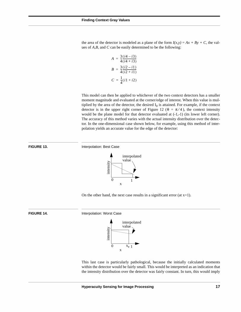
the area of the detector is modeled as a plane of the form I(x,y) = Ax + By + C, the val-ues of A,B, and C can be easily determined to be the following:

This model can then be applied to whichever of the two context detectors has a smallermoment magnitude and evaluated at the corner/edge of interest. When this value is mul-tiplied by the area of the detector, the desired I0 is attained. For example, if the contextdetector is in the upper right corner of Figure 12 ( ), the context intensitywould be the plane model for that detector evaluated at (-1,-1) (its lower left corner).The accuracy of this method varies with the actual intensity distribution over the detec-tor. In the one-dimensional case shown below, for example, using this method of inter-polation yields an accurate value for the edge of the detector:

FIGURE 13. Interpolation: Best Case

On the other hand, the next case results in a significant error (at x=1).

FIGURE 14. Interpolation: Worst Case

This last case is particularly pathological, because the initially calculated momentswithin the detector would be fairly small. This would be interpreted as an indication thatthe intensity distribution over the detector was fairly constant. In turn, this would imply

A34---

i4 i3–( )i4 i3+( )

---------------------=

B34---

i2 i1–( )i2 i1+( )

---------------------=

C14--- i1 i2+( )=

θ π 4⁄=

0 1

inte

nsity

x

interpolatedvalue

0 1

inte

nsity

x

interpolatedvalue

xe



that it would be safe to use for context (i.e., that the I0 of this detector could be used forIG1). If xe was close enough to 1.0, the constraint would be satisfied as well.However, using the I0 of this detector as context would lead to a very conspicuous error- essentially, the light and dark values for the edge would appear flipped (since thedesired dark context intensity would be a light value, and the light intensity would becalculated from this value and the total intensity to yield a dark value). As a result, afinal check is made before rendering the edge to make sure that the intensity of the lightside of the edge is actually higher than that of the dark side. If this is not the case, therewas clearly an error in attempting to find the context gray value, and the pixel is ren-dered as a non-edge (see the section on rendering non-edges).

Context in the Standard Detector Array

For the standard detectors, the freedom to choose either context intensity no longerexists. It is necessary to find the gray value on the side of the edge with the non-domi-nant area. This need arises from the macrodetector moment degeneracy presented ear-lier. In one dimension, the example below clearly demonstrates the problem:

FIGURE 15. One-dimensional Illustration of Macrodetector Degeneracy

If IG1 was used for context, we would effectively reproduce the situation shown in Fig-ure 11. On the other hand, if IG2 is used, the effective resulting distribution would be asfollows:

FIGURE 16. Figure 11 Intensity Distribution Normalized by IG2

This case is free from degeneracy, since the numerator of the macrodetector momentterm is no longer equal to the denominator. As long as there is an edge such that thenon-zero intensity (-G1 in this case) falls on more than one detector in each dimension,the macrodetector moment is not degenerate. The two-dimensional constraint for thiscan be realized by requiring that the non-zero intensity cover more than half of the mac-

ρ ρ0<

1.0

G1 G2

inte

nsit

y

0.5

1.0

-G1

inte

nsity

0.5

0



rodetector (the dominant area). To achieve this situation, the intensity of the non-domi-nant area must be used for context.

In order to determine whether the light or dark side of the edge covers the non-dominantarea, it is necessary to determine what the light and dark values are. To find this infor-mation, we must find an approximation of and . Fortunately, though the macrode-tector moment calculation is degenerate in terms of its uniqueness and sensitivity, itdoes not cause errors in that cross the quantization boundaries shown in Figure 11.

With the PSD array, we had only one choice for a context detector for any of the eight regions. Because we can get a total intensity (I0) value at twice this resolution for thestandard detector array (since the macrodetector of two by two standard detectors isbeing considered equivalent to one PSD), we have several choices for context. To sim-plify this discussion, the three groupings of neighboring detectors used for attainingcontext are shown below for the and cases (corresponding to regionsI and II in Figure 12). All other cases are rotationally symmetric to these. Note thatwhen more than one detector is used for context, the I0 values are averaged to attain thecontext gray value.

ρ θ

θ

θ

θ 0= θ π 4⁄=



FIGURE 17. Detector Groupings for Context Gray Values

To find the initial estimates of G1 (the dark side of the edge) and G2 (the light side), val-ues are determined for all three groupings shown for both the positive and negative directions. Whichever has the highest intensity value for the positive direction is chosenas G2, and whichever has the lowest intensity for the negative direction is chosen as G1.Because it is known that A1G1 + A2G2 = I0 and that A1 + A2 = Ad, it can be determinedwhich intensity covers the non-dominant area. The value for the corresponding I0 foundearlier is then used to transform the moments and determine the edge location. We havemade the assumption earlier on that only one edge can fall within a macrodetector. As aresult, the intensity of the dominant area can now be found exactly. This is because ifthe assumption holds, the dominant area must cover more than 50% of the detector area,and thus must fully cover at least one detector.

While the information of all four detectors is used to construct the edge model, only thecentral region of the macrodetector is rendered, as shown in the figure below. Instead ofiterating by macrodetector steps over the image, the algorithm steps detector by detec-

INSIDE:

OUTSIDE:

ALONG EDGES:

θ 0= θ π4---=

r

Rendering Non-Edges


tor, treating every possible grouping of four adjacent detectors as a macrodetector. Thisis because the macrodetector is most sensitive to edge position in the central region. Inaddition, if the entire macrodector were rendered, it would only be possible to have asingle edge running through the entire detector. On the other hand, if only the centralregion is rendered, the area of one macrodetector is rendered by eight different macro-detector groupings. Edges can thus be followed more closely, reducing the jagginess ofthe result, particularly when dealing with curved edges.

FIGURE 18. Rendered Area of Macrodetector

Rendering Non-Edges

After the recalculation of the moments, it is often the case that the magnitude of themoments is smaller than the threshold required to justify the edge model. In these cases,a variety of alternate models can be applied. The simplest among these is rendering theaverage gray value over the entire detector. This works well when the image fits themodel, i.e. there is no variation in the intensity over the area of the detector. However,often a detector for which the edge model does not apply still contains a significant gra-dient. The three independent pieces of information for the PSD and the four for the mac-rodetector are sufficient to take this gradient into account in rendering a non-edge. Theparticular models used, which make use of all the information available in each case, aredescribed below.

PSDs: the Plane Model

The plane model is used for the PSD array because it requires only three pieces of inde-pendent information: i.e., precisely what is available. This model has already been pre-sented in the earlier description of interpolating to find context gray values. Asdescribed there, this approach models the entire area of the detector as a single planeand can sometimes overshoot or undershoot the actual values at the edges of the detec-tor. As a result, the edges of the plane models of two adjacent detectors may not be thesame intensity, which can produce a false “edge” in the rendered image. Because thespatial extent of such a feature is only a single detector edge, it is usually not significant.If the area in the output image corresponding to a single detector is fairly large, though,the effect can be noticeable.

-1 1

-1

1

x

y

.5

.5

-.5

-.5

Performance


Standard Detectors: the Bilinear Model

The bilinear model requires the four pieces of independent information that are avail-able from a macrodetector. Green [4] develops this method in detail. It matches theaverage intensity of each detector at the exact center of the detector. The values betweencenters are linearly interpolated from the four nearest centers . The expression for theintensity of the rendered area of a macrodetector is thus as follows:

Note that at any detector center (i.e., any corner of the rendered area, such as x=0.5,y=0.5, etc.), the intensity matches that of the corresponding detector. As a result, thecorners and edges of adjacent rendered areas always match in intensity. This continuitygives the bilinear model a significant visual advantage over the plane model. In addi-tion, the total intensity over the area of each macrodetector is preserved.

Performance

Images have been divided into three categories to demonstrate various aspects of theperformance of these algorithms. These categories are continous tone, text/line art, andhalftone. A representative image from each category is shown in its original form and asprocessed for each of three algorithms: BBJJ for PSDs, BBJJ for standard detectors, andgray (i.e., the image area corresponding to a given is rendered with the average intensityincident on the detector - the rendering method used in typical scanning systems [5]).

Continuous Tone Images

Continuous tone images are those in which the intensity can vary continuously over theimage. This class of images is a particularly good test of the BBJJ algorithms, because itentails resolving edges of a variety of contrasts and as well accurately rendering non-edge areas. The original image is shown below:

I x y,( ) I11 x–

2-----------

1 y–2

----------- I2

x 1+2

------------ 1 y–

2-----------

I3x 1+

2------------

y 1+2

------------ I4

1 x–2

----------- y 1+

2------------

+ + +=

Performance


FIGURE 19. Original Continuous Tone Image

This image is now scanned by an array of 10 pixel by 10 pixel standard detectors, withthe average intensity for each detector rendered over that detector (gray model), result-ing in the following image.

FIGURE 20. Continuous Tone Image - Gray Model for 300 dpi Standard Detector Array

The BBJJ for standard detectors is then applied to this input:

Performance


FIGURE 21. Continuous Tone Image - BBJJ algorithm for 300 dpi Standard Detector Array

The same image is now shown for the BBJJ algorithm applied to a PSD array of thesame resolution:

FIGURE 22. Continuous Tone Image - BBJJ algorithm for 300 dpi PSD Array

To provide a fair comparison with regards to the amount of information available to thePSD, the gray and standard detector BBJJ are shown for a standard detector scanning attwice the resolution:

Performance


FIGURE 23. Continuous Tone Image - Gray Model for 600 dpi Standard Detector Array

FIGURE 24. Continuous Tone Image - BBJJ algorithm for 600 dpi pixel Standard Detector Array

Text and Line Art Images

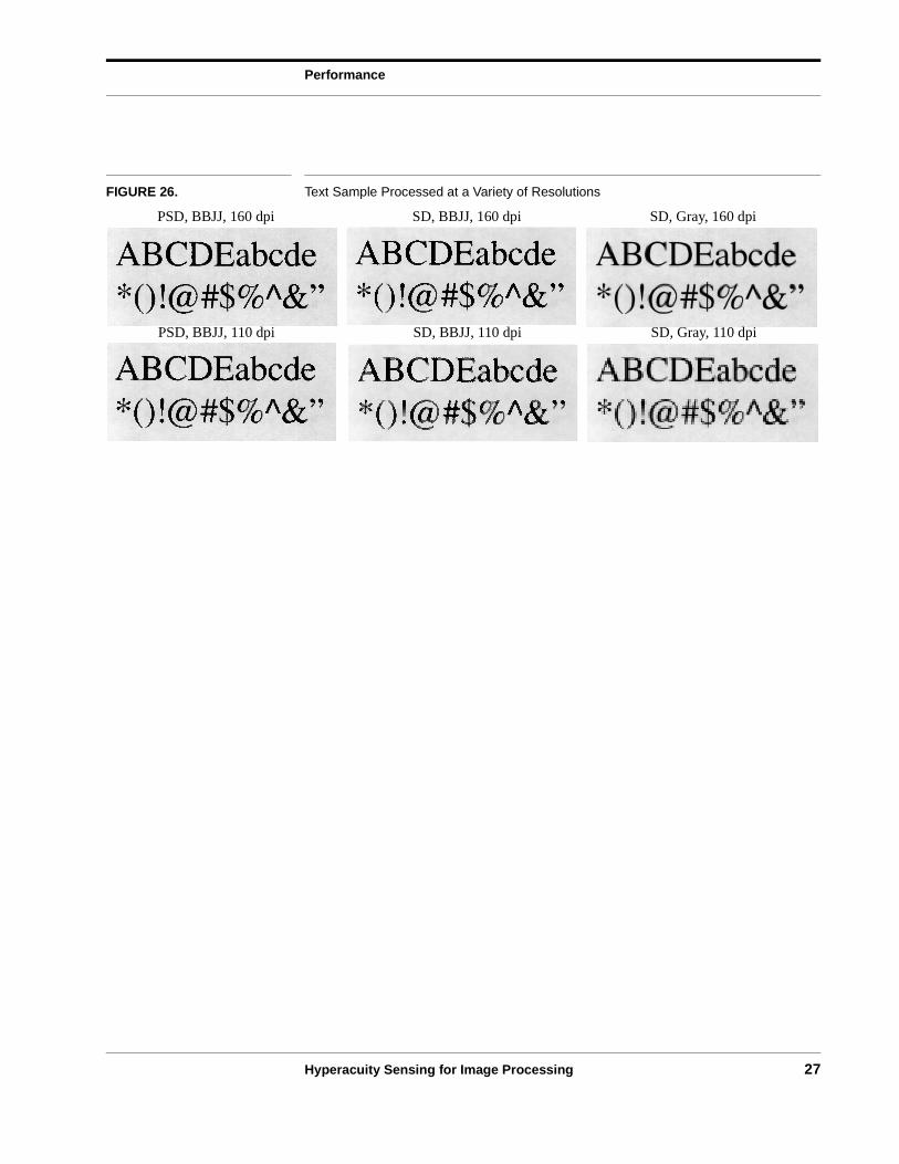
A second important class of images is text and line art. This type of image consists ofrelatively thin, high-frequency features on a background of constant or slowly varyingintensity. A sample of characters is shown processed by both versions of the BBJJ algo-rithm at a variety of resolutions. The spots-per-inch (spi) figure given is for a 10-pointfont. For a 20 point font, the spi would be halved, for a 5 point font, it would be dou-bled.

An important consideration is that the standard grayscale model often seems to workremarkably well on text images, even picking out some edges in certain characters. Thisoccurs because a significant number of the edges encountered in text are either horizon-tal or vertical with respect to the page. As a result, they often fall along the lines of thestandard detector. Edges then appear sharp since they follow the edges of iso-intensity

Performance


detectors. This effect quickly degenerates when the image is skewed, since the majorityof edges are then no longer horizontal or vertical.

FIGURE 25. Original Text Sample

Performance


FIGURE 26. Text Sample Processed at a Variety of Resolutions

PSD, BBJJ, 160 dpi SD, BBJJ, 160 dpi SD, Gray, 160 dpi


Performance


FIGURE 27. Text Sample Processed at a Variety of Resolutions (continued)

Halftoned Images

With halftone images, there are three regions of performance with regard to the scannerspot to printer spot (s:p) ratio. The first region is where the scanner spot size is on theorder of the printer spot size, where the ratio ranges from about one half to two. In thisregion, any gray-preserving algorithm reproduces the visually perceptible characteris-tics of the original image quite acurately. However, the BBJJ algorithm (for the PSD)has the advantage of being able to resolve individual halftone dots at this resolution.Though the effect of this is not readily visible if the image is rendered in gray, it can bebinarized (converted from gray into black and white) without significant loss of quality.The gray model cannot be binarized in this manner without a serious loss in quality. Thegray and binarized version of each algorithm are shown below for an image with aprinter spot size of 4 pixels and a scanner spot size of 7 pixels. Note, however, that theeffective s:p ratio for macrodetectors in the standard detector BBJJ case is twice that forsingle detectors (i.e., 14:4 instead of 7:4).

PSD, BBJJ, 80dpi SD, BBJJ, 80 dpi SD, Gray, 80 dpi



PSD: Position Sensitive DetectorSD: Standard Detector

Performance


FIGURE 28. Original Halftoned Image

FIGURE 29. Grayscale Results of Algorithms on Halftoned Image (2:1 s:p ratio)

FIGURE 30. Binarized Results of Algorithms on Halftoned Image (2:1 s:p ratio)

In the second region (shown below), the scanner spot is three to five times the printerspot size. This is the most volatile of the three regions in that slight changes in the scan-ner spot size or the alignment of the image can produce severe Moire (aliasing) patterns(see Hall [5] and Rozenfield [12] for descriptions and explanations of this effect). Thisresult occurs in all three of the algorithms, and is not any more pronounced for the BBJJ

PSD, BBJJ SD, BBJJ SD, Gray


Performance


algorithm than with the simple gray model. The result of each algorithm with a scannerspot size of 15 pixels is shown below.


The third region (shown below) is where the scanner spot is about an order of magni-tude or more times greater than the printer spot size. At this resolution, at least oneentire halftone cell is under each detector, resulting in the average gray value of thedetector being the original gray value that was rendered with the halftone distribution.The image looks increasingly like a continuous tone image as the s:p ratio increases, andthe performance goes up accordingly. The BBJJ algorithm is quite effective in thisregion because it can find edges between the regions of these halftoned grays, just as itcould with continuous tone images. The result of each algorithm with a scanner spotsize of 30 pixels is shown below. Note that the blurring effect in the border of the stan-dard detector BBJJ case occurs because there are no detectors outside this region withwhich a macrodetector can be composed. As a result, a half-detector width region oneach border of the image is rendered using the non-edge model. The effect is particu-larly pronounced here because the area of a detector is quite large with respect to theimage size.




Discussion


Discussion

It is worth reviewing at this point the major goal of hyperacuity sensing - the correctrendering of visually significant features of the original image. It is not possible to rer-ender a 600 spi checkerboard with the output from a 200 spi PSD array with the BBJJalgorithm, nor is it necessary in order to satisfy the goal above - the algorithm wouldproduce the same uniform gray that the human eye would see from a normal viewingdistance. This goal is not sufficient for all applications of image scanning. For example,the content of an image in which the halftoning pattern itself contains encoded informa-tion cannot be retrieved. However, for the vast majority of images that are scanned, it isvisual significance that is crucial and not pixel for pixel accuracy. In other words, if textis legible on a page, it should still be legible in the scanned image, but if there is a stripethat appears gray which is actually rendered with a high-resolution halftone on the page,it is sufficient to render it with a single gray tone. With this expanded view of the stan-dard in mind, the performance of the BBJJ algorithm can be more practically judged.

Advantages

Though the performance of the BBJJ algorithm was shown on several distinct classes ofimages, it is crucial to note that no parameters were set differently for the differentimages. In other words, if all of the images were put together onto a single page, thealgorithm would have the same performance as shown above for each part of such aconglomerate image. This is because the algorithm uses only extremely local contextinformation - within a radius of one detector/macrodetector - to determine the represen-tation for a given detector. As opposed to traditional edge detection and resolution meth-ods which attempt to parametrize edges spanning large areas in the image (see, forexample, Haralick [6] and Hall [5]), the BBJJ algorithm only represents and rendersedges on a local scale. As a result, the errors it makes are also only on a local scale. Inaddition, because the algorithm works in a single pass over the image, local mistakescannot propagate outside the detector area. The single-pass aspect is also beneficialfrom a computational perspective, in that the time required to process an image is lin-early related to the size of the image and independent of the image’s complexity.

Another important aspect of the algorithm is that it is intensity-conserving on the detec-tor level for the PSD case and on the macrodetector level for the standard detector case.In other words, the total intensity of the algorithm’s output representation for a givendetector/macrodetector is always equal to the total intensity incident on the detector/macrodetector. This fact can be easily verified by examining the algorithms above. Con-serving the intensity is crucial in preserving the appearance of the image. At a largeenough viewing distance for a given size of image area, two areas that contain the sametotal intensity appear the same to the eye. The output of the BBJJ algorithm thus appearsvery similar to the gray model at the viewing distance corresponding to the area of onedetector/macrodetector, regardless of how poorly the algorithm chooses and parame-trizes the edge and continuous models. The key benefit of this is that at some viewingdistance, the output of the algorithm will appear indistinguishable from the original.Though details may be lost and moire patterns may appear, the conservation of gray atthe detector level prevents the algorithm from making gross errors over a large region ofthe image.

Discussion


The examples in the performance section have shown several situations where the BBJJalgorithm can reconstruct visually significant details in the image. What may not be evi-dent, though, are the inherent benefits of extracting an edge representation from thedata. The final output of the BBJJ algorithm for each detector-sized area is a set of fourparameters, describing either the position, orientation, and intensity levels of an edge orthe coefficients for a continuous description (either plane model or bilinear model). Thefact that this is an analytic description of the image under the detector’s area makesoperations such as scaling and rotation simple: the representation can be held constant,while the area of the output image corresponding to each detector can be scaled, rotated,etc. As long as a transformation can be found between a point on the original location ofthe detector to the new coordinate system of the rendered image, the rendering can beperformed on these transformed coordinates. This is not the case in the typical scannedimage representation, in which only the average intensity for each detector is extractedfrom the scan (i.e., a grayscale representation). While edges in the image may appearsmooth when each detector corresponds to one or a few pixels in the image, the squareshape of each detector’s area becomes apparent as the image is scaled (see, for example,Figure 20).

In addition, the edge/continuous model representation can be used to obtain “segmenta-tion” information about an image, where segmentation refers to the process of dividingan image into several regions according the image content (i.e., regions of text, regionsof halftoned images, etc.). Because the system developed in this study did not requiresegmentation for its operation, it was not a primary concern. However, it was found thatinformation resulting from the BBJJ algorithm could be quite useful in performing seg-mentation. It was observed that the output of the algorithm for text and line art imagescontained a large fraction of detectors with edges, while continuous tone images had amuch smaller fraction. The fraction of edge-containing detectors for a given area of animage could thus be used to determine whether it contained text or illustrations. Thisinformation could be very useful if the BBJJ algorithm was being used as an image pre-processor for a system that did require segmentation, such as an OCR system.

Problems

There are several issues concerning the applicability of the BBJJ algorithm in scanningsystems. The first of these concerns the output to scan (o:s) ratio. If the area of eachdetector is rendered on a group of n by n pixels in the output device, this ratio is n.Clearly, if this ratio is not at least two, the BBJJ algorithm provides no benefit whatso-ever, since a sub-detector edge cannot be rendered in a single pixel of the output device.Since the output device of interest is often a printer, the ratio must be even higher, sincemost printers (film and color printers excepted) can produce only binary intensity for agiven pixel and need to compose several pixels to produce a gray value. This means thatfor a significant performance advantage, the output device must have a resolution sev-eral times higher than that of the standard 300 spi scanner. This implies that the algo-rithm is not very useful for images scanned on a standard 300 spi scanner and printed ona 600 spi binary printer. However, printer technology is advancing rapidly in terms ofboth ability and cost, and much higher resolution printers will soon be readily available.This concern can also be countered, though, by considering the many additional abilitiesof a system using BBJJ. For instance, if the image was to be scaled by some factor, theo:s ratio would be increased by the scale factor and the details reconstructed by the algo-rithm would be of direct benefit in the output image. Another approach is to consider

Discussion


the possibility of using cheaper, lower resolution scanners to deliver the same or betterimage quality using the BBJJ algorithm. This method also increases the effective o:sratio.

The other class of problems involves limitations and artifacts produced by the BBJJalgorithm. Because the system requires clear context values to be able to correctly ren-der edges, an image that has a very high spatial density of edges or edge-like featurescannot be accurately rendered: the corresponding regions will be rendered as continuousapproximations to the variation. As discussed earlier in the description of the algorithm,this will only occur when more than two edges occur within one detector/macrodetector.The scanning system thus must have a resolution such that desired features (i.e., a givensize/font of text) do not exceed this constraint.

An additional problem with the algorithm arises from the fact that edges are alwaysmodeled as linear. If there is an edge of high curvature that passes through several adja-cent detectors, the algorithm will produce the best linear fit for each detector to its corre-sponding region of the curve. However, in some cases this results in the edges beingmismatched at detector boundaries. This same problem can occur along a relativelystraight edge if there is noise in the image or the detector measurements. This problemcan be corrected by doing a second pass which constrains the edges of neighboringedge-containing detectors to match. However, this would cause two significant prob-lems - first, it would increase the time required to run the alogrithm, and second,increase the effective context area on average to twice its current size (since all of thecontext of the relevant neighbors would be taken indirectly into account).

Future Directions

The most important next step to be undertaken in this study is the production of full-sized PSD arrays and the investigation of their properties. It must be determinedwhether the effects of noise and the system required to support such an array supersedethe benefits of the BBJJ PSD algorithm.

Another interesting direction to proceed is the extraction of “macro” information fromthe BBJJ algorithm’s output representation. A method for image segmentation hasalready been presented: it has been tested in a very basic sense; it would be worthwhileto fully develop this idea and determine the quality of segmentation that can be per-formed. Similarly, it may be possible to deskew a text image using information from theBBJJ algorithm. As mentioned earlier in the discussion of the algorithm’s performanceon text images, most fonts tend to have a large number of vertical and horizontal lines inthem. As a result, the distribution of the parameter in edge-containing detectorsshould have peaks for the horizontal and vertical directions of the text. Additionally, it isknown that these peaks should be 90 degrees apart from each other. The correspondingpair of peaks should thus be fairly easy to find. Because the smaller of these thetas cor-respond to the orientation of the text lines, the image can be deskewed by rotating itback by this angle. Both the segmentation and the deskewing algorithm are worth sig-nificant further investigation.

θ

Conclusions


Conclusions

It was found through this study that hyperacuity sensing can be beneficial in recon-structing visually significant sub-detector-sized features in scanned images. While per-formance varied depending on the size and spatial density of image features in relationto the size of the detector elements, the hyperacuity sensing algorithm performed at leastas well as the standard gray algorithm, and in most cases was able to accurately rendermany sub-detector sized features. In addition, it was found that composing informationfrom four standard detectors to simulate the hyperacuity sensing properties of the PSDdetectors was fairly successful. Significant improvements over the original scannedresult (standard detector data) could be attained through processing by the BBJJ algo-rithm. Since this latter approach works with the information available from exisitingdetector elements, it could be easily applied in software to the output of current scan-ning systems.

References

[1] Bloomer, J., and Abdel-Malek, A. “Visually Optimized Image Reconstruction,”SPIE vol. 1249: Proc. Human Vision and Electronic Imaging: Models, Methods,and Applications. 12-14 Feb., 1990. pp. 330-335.

[2] Fahle, M. “Parallel, Semi-Parallel, and Serial Processing of Visual Hyperacuity.”SPIE vol. 1249: Proc. Human Vision and Electronic Imaging: Models, Methods,and Applications. 12-14 Feb., 1990. pp. 147-159.

[3] Fahle, M. “Visual Hyperacuity: Parallel vs. Serial Processing.” Invest. Opthal. Vis.Sci. Suppl. 28, pp. 361-365, 1987.

[4] Green, W. B. Digital Image Processing, 2nd ed. Reinhold: New York, 1989,pp.118-120.

[5] Hall, Ernest. Computer Image Processing and Recognition. Academic Press: NewYork, 1979. pp. 93-94.

[6] Haralick, R.and Shapiro, L. “Chapter 10: Image Segmentation” and “Chapter 11:Arc Extraction and Segmentation.” Computer and Robot Vision. Addison-Wesley:New York, 1992.

[7] Lennie, P. and D’Zmura, M. “Mechanisms of Color Vision.” CRC Critical Reviewsin Neurobiology 3, 1988. pp. 333-400.

[8] Marr, D., and Hildreth, E. “Theory of Edge Detection.” Proc. Soc. Lond. B. 207,1980.

[9] Martinez-Uriegas, Eugenio. “Spatiotemporal Multiplexing of Chromatic and Ach-romatic Information in Human Vision.” SPIE vol. 1249: Proc. Human Vision andElectronic Imaging: Models, Methods, and Applications. 12-14 Feb., 1990. pp.178-199.

[10] Nishihara, H. K., and Poggio, T. “Hidden Cues in Random Line Stereograms,” A.I.Memo No. 737. MIT: Cambridge, August 1993.

[11] Pearlman, W. A. “A Visual System Model and a New Distortion Measure in theContext of Image Processing.” Journal Opt. Society of America, Vol. 68(3). March1978. pp.374-385.

[12] Rozenfield, A. and Kak, A. Digital Picture Processing. Academic Press: NewYork, 1976. pp. 79-81.

Documents

Hyperacuity Sensing for Image Processingalumni.media.mit.edu/~sbasu/papers/SB_thesis.pdf · development and effectiveness of a scanning system that has a similarly varying ... S.B