Embed Size (px)
Citation preview
HAL Id: tel-00796108https://tel.archives-ouvertes.fr/tel-00796108
Submitted on 7 May 2013
HAL is a multi-disciplinary open accessarchive for the deposit and dissemination of sci-entific research documents, whether they are pub-lished or not. The documents may come fromteaching and research institutions in France orabroad, or from public or private research centers.
L’archive ouverte pluridisciplinaire HAL, estdestinée au dépôt et à la diffusion de documentsscientifiques de niveau recherche, publiés ou non,émanant des établissements d’enseignement et derecherche français ou étrangers, des laboratoirespublics ou privés.
Hyperspectral image representation and Processing withBinary Partition Trees
Silvia Valero
To cite this version:Silvia Valero. Hyperspectral image representation and Processing with Binary Partition Trees. ImageProcessing. Université de Grenoble, 2011. English. <tel-00796108>

THÈSE Pour obtenir le grade de
DOCTEUR DE L’UNIVERSITÉ DE GRENOBLE et L’UNIVERSITAT POLITÈCNICA DE CATALUNYA
Spécialité : Signal, Image, Parole et Télécom!
Arrêté ministériel : 7 août 2006
Présentée par
Silvia, VALERO VALBUENA Thèse dirigée par Jocelyn CHANUSSOT et
codirigée par Philippe SALEMBIER préparée au sein du Grenoble Images Parole Signal Automatiue Laboratoire (Gipsa-Lab)
dans "#$%&"'!(&%)&*+"'!,!-"'%)*&./01'!2!-"'%)*&)'%3./01'2!41)&5+)/01'2!6*+/)'5'.)!71!8/9.+"!:
Arbre de partition binaire : Un nouvel outil pour la représentation hiérarchique et l’analyse des images hyperspectrales Thèse soutenue publiquement le 9 decembre 2011 devant le jury composé de :
M. Jean, SERRA Professeur Emerite, ESIEE Paris, Président du jury
M. Antonio, PLAZA Associate Professor, Escuela Politecnica de Caceres-University of Extremadura, Rapporteur
Mme. Josiane, ZERUBIA DR INRIA, INRIA Sophia Antipolis Méditerranée, Rapportrice
M. Carlos, LOPEZ-MARTINEZ Assistant Professeur, Universitat Politecnica de Catalunya, Examinateur
M. Hugues, TALBOT Professeur associé, ESIEE Paris, Examinateur
M. Jesus, ANGULO Chargé de recherche, Centre de Morphologie Mathématique, MINES-ParisTech, Examinateur

A mis padres, a mi hermano y a Xavi.
Por su apoyo, comprensión y paciencia durante todos estos años.

2

Acknowledgements
Mes remerciements vont tout d’abord aux membres du jury qui ont eu l’amabilité et la gentillesse
d’évaluer mon travail. Je souhaite aussi remercier mes deux directeurs de thèse, Philippe Salem-
bier et Jocelyn Chanussot.
Merci Jocelyn de m’avoir fait confiance dès le départ de cette course. Merci Philippe, sans toi
la réalisation de ce projet n’aurait également pas été envisageable. Merci pour ces ans pendant
lesquels j’ai beaucoup appris à votre côté.
Gracias a mi padres, por educarme y enseñarme a ser como soy. Gracias a mi hermano, con quien
tanto he compartido. Gracias a Xavi, por estos ocho años a mi lado.
Por último, gracias a todos mis amigos por ser mi segunda familia.

4
Abstract
The optimal exploitation of the information provided by hyperspectral images requires the devel-
opment of advanced image processing tools. Therefore, under the title Hyperspectral image rep-
resentation and Processing with Binary Partition Trees, this PhD thesis proposes the construc-
tion and the processing of a new region-based hierarchical hyperspectral image representation:
the Binary Partition Tree (BPT). This hierarchical region-based representation can be interpreted
as a set of hierarchical regions stored in a tree structure. Hence, the Binary Partition Tree succeeds
in presenting: (i) the decomposition of the image in terms of coherent regions and (ii) the inclusion
relations of the regions in the scene. Based on region-merging techniques, the construction of BPT
is investigated in this work by studying hyperspectral region models and the associated similarity
metrics. As a matter of fact, the very high dimensionality and the complexity of the data require
the definition of specific region models and similarity measures. Once the BPT is constructed,
the fixed tree structure allows implementing efficient and advanced application-dependent tech-
niques on it. The application-dependent processing of BPT is generally implemented through a
specific pruning of the tree. Accordingly, some pruning techniques are proposed and discussed
according to different applications. This Ph.D is focused in particular on segmentation, object de-
tection and classification of hyperspectral imagery. Experimental results on various hyperspectral
data sets demonstrate the interest and the good performances of the BPT representation.

6
Contents
1 Introduction 9
1.1 Hyperspectral imaging . . . . . . . . . . . . . . . . . . . . . . . . . . . . . . . . . . . 10
1.2 Binary Partition Trees . . . . . . . . . . . . . . . . . . . . . . . . . . . . . . . . . . . . 11
1.3 Objectives . . . . . . . . . . . . . . . . . . . . . . . . . . . . . . . . . . . . . . . . . . 15
1.4 Thesis Organization . . . . . . . . . . . . . . . . . . . . . . . . . . . . . . . . . . . . . 17
2 State of the art 19
2.1 Hyperspectral image processing . . . . . . . . . . . . . . . . . . . . . . . . . . . . . 20
2.1.1 Classification techniques incorporating spatial constraints . . . . . . . . . . 21
2.1.2 Traditional imagery techniques extended to HSI . . . . . . . . . . . . . . . . 25
2.2 Hierarchical region-based processing using trees . . . . . . . . . . . . . . . . . . . . 33
2.2.1 Definition of the tree structure . . . . . . . . . . . . . . . . . . . . . . . . . . 35
2.2.2 First hierarchical tree representations . . . . . . . . . . . . . . . . . . . . . . 36
2.2.3 BPT Literature . . . . . . . . . . . . . . . . . . . . . . . . . . . . . . . . . . . 38
2.3 Conclusions . . . . . . . . . . . . . . . . . . . . . . . . . . . . . . . . . . . . . . . . . 39
3 BPT construction 41
3.1 Introduction . . . . . . . . . . . . . . . . . . . . . . . . . . . . . . . . . . . . . . . . . 42
3.2 Region Model . . . . . . . . . . . . . . . . . . . . . . . . . . . . . . . . . . . . . . . . 45
3.2.1 First-order parametric model . . . . . . . . . . . . . . . . . . . . . . . . . . . 46
3.2.2 Non parametric statistical Region Model . . . . . . . . . . . . . . . . . . . . 47
3.3 Merging Criterion . . . . . . . . . . . . . . . . . . . . . . . . . . . . . . . . . . . . . . 55
3.3.1 Measures associated to the first-order parametric model . . . . . . . . . . . 59
3.3.2 Measures associated to the non parametrical statistical region model . . . . 61
3.3.3 Similarity measure via Multidimensional Scaling . . . . . . . . . . . . . . . 64
3.4 Experimental Evaluation . . . . . . . . . . . . . . . . . . . . . . . . . . . . . . . . . . 71
3.4.1 Quality measures between partitions . . . . . . . . . . . . . . . . . . . . . . 71
3.4.2 Data Sets Definition . . . . . . . . . . . . . . . . . . . . . . . . . . . . . . . . 73
3.4.3 Experiment 1: Evaluation of BPT hierarchical levels . . . . . . . . . . . . . . 78
3.4.4 Experiment 2: Evaluation of Ds selection . . . . . . . . . . . . . . . . . . . . 93
3.5 Conclusions . . . . . . . . . . . . . . . . . . . . . . . . . . . . . . . . . . . . . . . . . 94

8 CONTENTS
4 BPT Pruning Strategies 97
4.1 Introduction . . . . . . . . . . . . . . . . . . . . . . . . . . . . . . . . . . . . . . . . . 98
4.2 Supervised Hyperspectral Classification . . . . . . . . . . . . . . . . . . . . . . . . 103
4.2.1 Populating the BPT . . . . . . . . . . . . . . . . . . . . . . . . . . . . . . . . 103
4.2.2 Pruning Decision . . . . . . . . . . . . . . . . . . . . . . . . . . . . . . . . . . 105
4.2.3 Experimental results . . . . . . . . . . . . . . . . . . . . . . . . . . . . . . . . 107
4.3 Segmentation by Energy Minimization Strategy . . . . . . . . . . . . . . . . . . . . 115
4.3.1 The D(N ) definition . . . . . . . . . . . . . . . . . . . . . . . . . . . . . . . . 118
4.3.2 Homogeneity measure . . . . . . . . . . . . . . . . . . . . . . . . . . . . . . 118
4.3.3 Experimental Results . . . . . . . . . . . . . . . . . . . . . . . . . . . . . . . . 119
4.4 Segmentation by recursive spectral graph partitioning . . . . . . . . . . . . . . . . . 124
4.4.1 The BPT node weight WN . . . . . . . . . . . . . . . . . . . . . . . . . . . . 124
4.4.2 Local Branch partitioning . . . . . . . . . . . . . . . . . . . . . . . . . . . . . 126
4.4.3 Experimental Results . . . . . . . . . . . . . . . . . . . . . . . . . . . . . . . . 130
4.5 Object detection . . . . . . . . . . . . . . . . . . . . . . . . . . . . . . . . . . . . . . . 135
4.5.1 Detection of roads . . . . . . . . . . . . . . . . . . . . . . . . . . . . . . . . . 136
4.5.2 Detection of buildings . . . . . . . . . . . . . . . . . . . . . . . . . . . . . . . 137
4.5.3 Experimental Results . . . . . . . . . . . . . . . . . . . . . . . . . . . . . . . . 138
4.6 Conclusions . . . . . . . . . . . . . . . . . . . . . . . . . . . . . . . . . . . . . . . . . 140
5 Conclusions 143
6 Appendix 147
6.1 Tree complexity . . . . . . . . . . . . . . . . . . . . . . . . . . . . . . . . . . . . . . . 148
6.2 Acronyms . . . . . . . . . . . . . . . . . . . . . . . . . . . . . . . . . . . . . . . . . . 153
6.3 Mathematical Appendix: Association measures . . . . . . . . . . . . . . . . . . . . 155
6.4 Hierarchical levels obtained by Pavia University data set . . . . . . . . . . . . . . . 158
6.5 List of Publications . . . . . . . . . . . . . . . . . . . . . . . . . . . . . . . . . . . . . 159
7 Résumé en français 161
1Introduction
Hyperspectral imaging, also known as imaging spectroscopy, corresponds to the acquisition of
a set of images representing the information contained in a large portion of the electromagnetic
spectrum. In contrast to human vision which is restricted to some wavelengths, these spectral
imaging systems have the capability of viewing electromagnetic radiation ranging from ultravi-
olet to infrared. With this additional spectral (or color) information, these images exhibit greatly
improved color differentiation as compared to conventional color imaging. This new source of
information implies an important difference between hyperspectral and traditional imagery. The
main difference is that hyperspectral images are composed by hundreds of bands in the visible
range and other portions of the electromagnetic spectrum. Therefore, hyperspectral imagery al-
lows sensing radiation in a spectral range where human eyes cannot.
Hyperspectral imaging is related to multispectral imaging, however, it exists an important differ-
ence between the number of spectral bands. Multispectral images usually contain a set of up to
ten spectral bands that moreover are typically not contiguous in the electromagnetic spectrum.
Contrarily, hyperspectral images have a large number of narrow spectral bands (usually several
hundreds) being captured by one sensor in a contiguous spectral range. Hence, hyperspectral
imaging often provides results not achievable with multispectral or other types of imagery. The
characterization of images based on their spectral properties has led to the use of this type of im-
ages in a growing number of real-life applications.
In remote sensing, many applications such as mineralogy, biology, defense or environmental mea-
surements have used of the potential of these images. In a different field, some techniques have
10 Chapter 1. Introduction
used hyperspectral data in order to study food quality, safety evaluation and inspection. Also,
in medical research, these images are used to analyze reflected and fluorescent light applied to
the human body. In this context, hyperspectral imaging is an emerging technique which serves
as a diagnostic tool as well as a method for evaluating the effectiveness of applied therapies. In
planetary exploration these data are also used to obtain geochemical information from inaccessi-
ble planetary surfaces within the solar system.
The traditional hyperspectral image representation involves an array of spectral measurements
on the natural scene where each of them corresponds to a pixel. This most elementary unit on the
image, provides an extremely local information. Furthermore, besides the scale issue, the pixel-
based representation also suffers from the lack of structure. As a result, hyperspectral image
processing at the pixel level has to face major difficulties in terms of scale: the scale of representa-
tion is most of the time far too low with respect to the interpretation or decision scale.
Hence, the general aim of this thesis is the construction and the exploitation of a new hyperspec-
tral image representation. The goal of this new representation is to describe the image as a set of
connected regions instead of as a set of individual pixels. This abstraction from pixels to regions
is achieved by Binary Partition Trees. These region-based image representations are presented in
this thesis as an attractive and promising solution to handle the low level representation problem.
In this framework, this first chapter is starting by the basic background concerning this Phd re-
search. Firstly, a brief description of the hyperspectral imagery and the Binary Partition Tree
representation is presented in the following. Afterward, the main objectives and the organization
of this thesis are described.
1.1 Hyperspectral imaging
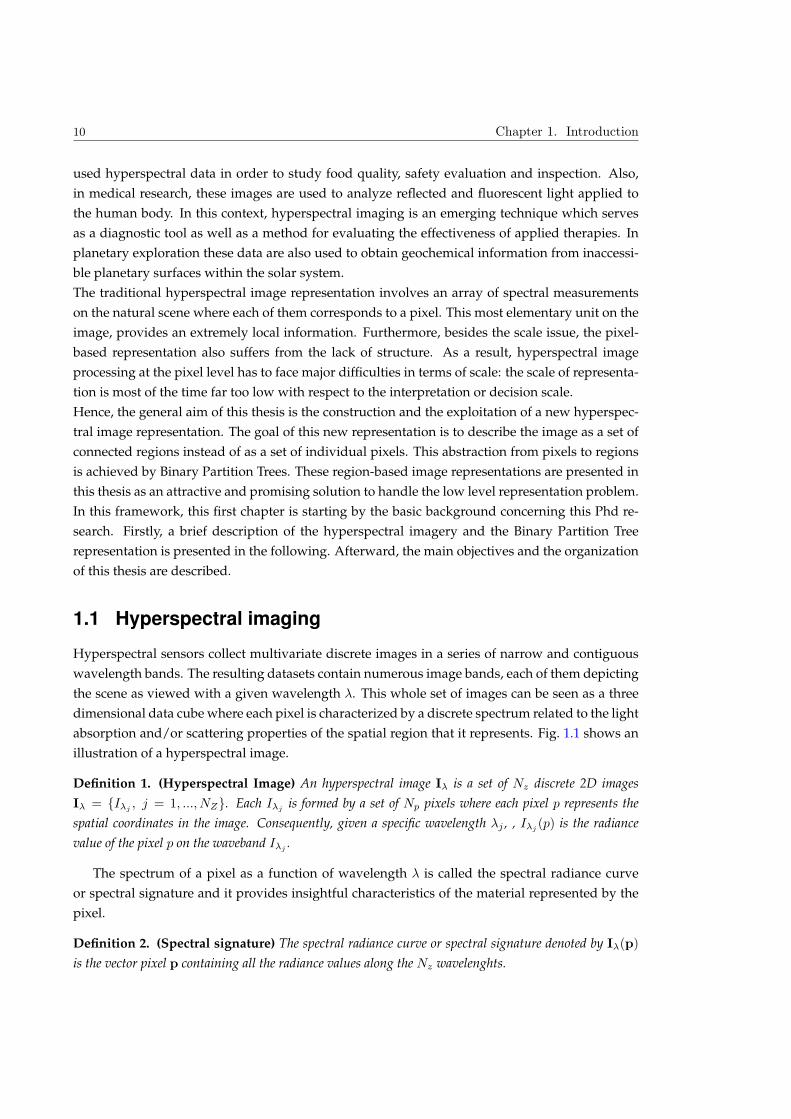
Hyperspectral sensors collect multivariate discrete images in a series of narrow and contiguous
wavelength bands. The resulting datasets contain numerous image bands, each of them depicting
the scene as viewed with a given wavelength λ. This whole set of images can be seen as a three
dimensional data cube where each pixel is characterized by a discrete spectrum related to the light
absorption and/or scattering properties of the spatial region that it represents. Fig. 1.1 shows an
illustration of a hyperspectral image.
Definition 1. (Hyperspectral Image) An hyperspectral image Iλ is a set of Nz discrete 2D images
Iλ = Iλj, j = 1, ..., NZ. Each Iλj
is formed by a set of Np pixels where each pixel p represents the
spatial coordinates in the image. Consequently, given a specific wavelength λj , , Iλj(p) is the radiance
value of the pixel p on the waveband Iλj.
The spectrum of a pixel as a function of wavelength λ is called the spectral radiance curve
or spectral signature and it provides insightful characteristics of the material represented by the
pixel.
Definition 2. (Spectral signature) The spectral radiance curve or spectral signature denoted by Iλ(p)
is the vector pixel p containing all the radiance values along the Nz wavelenghts.
1.2 Binary Partition Trees 11
X
y
そ
そ!"そ#
そ$"
!"#
$%&'%()*
+%,*-*(./01そ
そ2
そ3!"#
Figure 1.1: Illustration of a hyperspectral image
The price of the wealth of information provided by hyperspectral images is a huge amount of
data that cannot be fully exploited using traditional imagery analysis tools. Hence, given the wide
range of real-life applications, a great deal of research is devoted to the field of hyperspectral data
processing [1]. A hyperspectral image can be considered as a mapping between a 2D spatial space
to a spectral space of dimension Nz . The spectral space is important because it contains much
more information about the surface of target objects than what can be perceived by human vision.
The spatial space is also important because it describes the spatial variations and correlation in
the image and this information is essential to interpret objects in natural scenes. Hyperspectral
analysis tools should take into account both the spatial and the spectral spaces in order to be
robust and efficient. However, the number of wavelengths per pixel and the number of pixels per
image, as well as the complexity of jointly handling spatial and spectral correlation explain why
this approach is still a largely open research issue for effective and efficient hyperspectral data
processing.
Hyperspectral image processing highly desired goals include automatic content extraction and
retrieval. These aims to obtain a complete interpretation of a scene are addressed by supervised
or unsupervised pixel level analysis which still requires a remote sensing analyst to manually
interpret the pixel-based results to find high-level structures. This is because there is still a large
semantic gap between the outputs of commonly used models and high-level user expectations.
The limitations of pixel-based models and their inability in modeling spatial content motivated
the research on developing algorithms for region-based analysis.
1.2 Binary Partition Trees
Binary Partition Tree (BPT)[15] is a hierarchical region-based representation, which can be inter-
preted as a set of hierarchical regions stored in a tree structure. A tree structure is well suited for
representing relationships among data in a hierarchical way.
An easy example of the hierarchical organization is the structure followed by the files and folders
12 Chapter 1. Introduction
in a computer. The hierarchy between the folders clearly offers to the user the ability to efficiently
manage filesand the stored information.
In image analysis, tree structures can be used as a hierarchical data organization in a similar
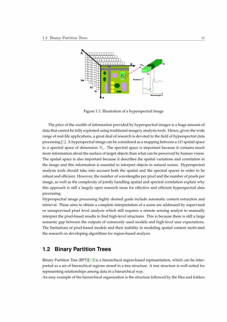
way. An example of such tree representations is the Binary Partition Tree, where the tree nodes
represent image regions and the branches represent the inclusion relationship among the nodes.
Fig. 1.2 is an illustration of a BPT which shows the hierarchical representation offered by this rep-
resentation.
In this tree representation, three types of nodes can be found: Firstly, leaves nodes representing
the original regions of the initial partition; secondly, the root node representing the entire image
support and finally, the remaining tree nodes representing regions formed by the merging of their
two child nodes corresponding to two adjacent regions. Each of these non leaf node has at most
two child nodes, this is why the BPT is defined as binary.
Figure 1.2: Example of hierarchical region-based representation using BPT
The BPT construction is often based on an iterative bottom-up region merging algorithm.
Starting from individual pixels or any other initial partition, the region merging algorithm is an
iterative process in which regions are iteratively merged. Each iteration requires three different
tasks: 1) the pair of most similar neighboring regions is merged, 2) a new region containing the
union of the merged regions is formed, 3) the algorithm updates the distance between the new
created region with its neighboring regions.
Working with hyperspectral data, the definition of a region merging algorithm is not straight-
forward. Theoretically, a pixel in an hyperspectral image is a spectrum representing a certain
ground cover material. Consequently, regions formed by pixels belonging to the same material
are expected to be formed by an unique reflectance curve. Unfortunately, this assumption is not
true since it exists a large spectral variability in a set of spectra formed by one given material.
In the case of remote sensing images, this variability is introduced by several factors such as the
noise resulting from atmospheric conditions, the sensor influence, non direct reflexion or the illu-
mination effects.
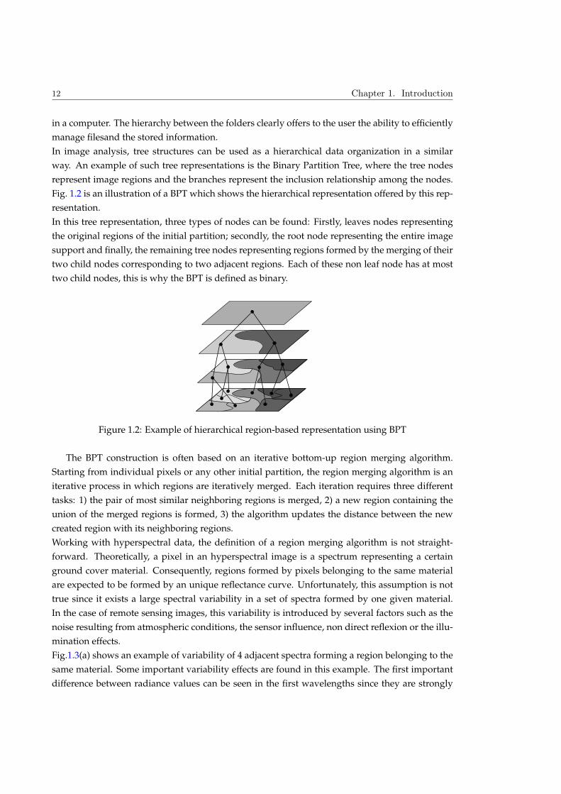
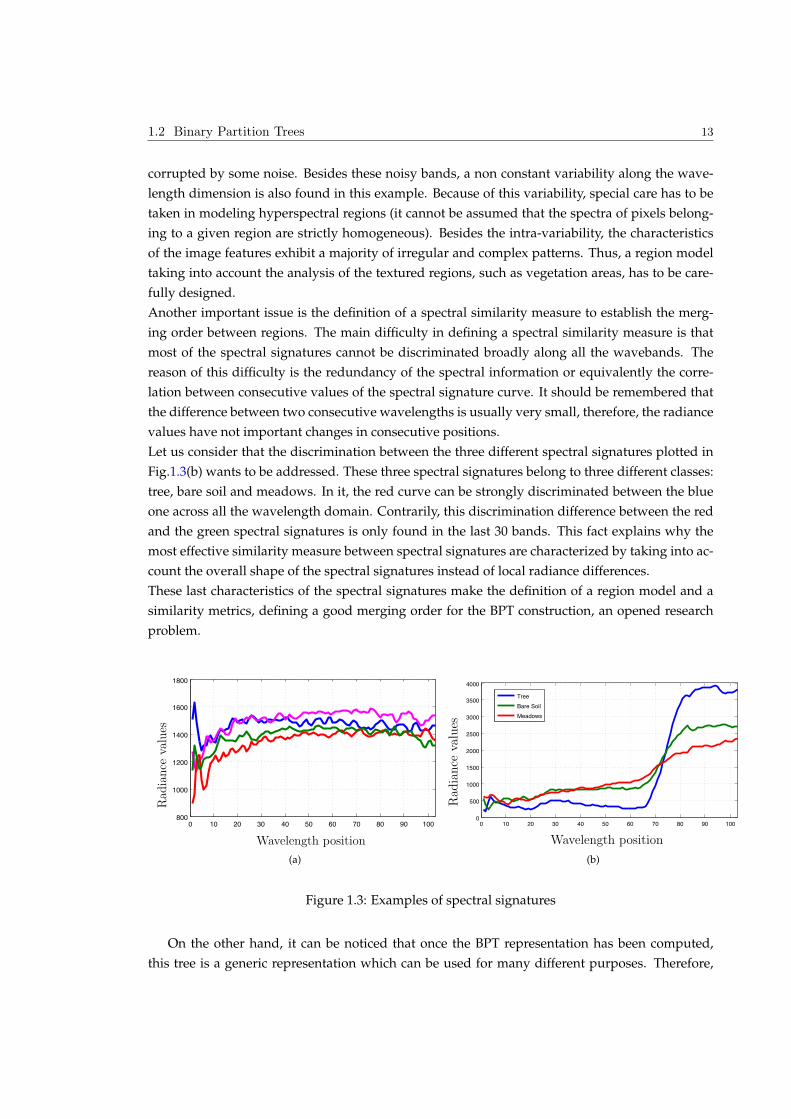
Fig.1.3(a) shows an example of variability of 4 adjacent spectra forming a region belonging to the
same material. Some important variability effects are found in this example. The first important
difference between radiance values can be seen in the first wavelengths since they are strongly
1.2 Binary Partition Trees 13
corrupted by some noise. Besides these noisy bands, a non constant variability along the wave-
length dimension is also found in this example. Because of this variability, special care has to be
taken in modeling hyperspectral regions (it cannot be assumed that the spectra of pixels belong-
ing to a given region are strictly homogeneous). Besides the intra-variability, the characteristics
of the image features exhibit a majority of irregular and complex patterns. Thus, a region model
taking into account the analysis of the textured regions, such as vegetation areas, has to be care-
fully designed.
Another important issue is the definition of a spectral similarity measure to establish the merg-
ing order between regions. The main difficulty in defining a spectral similarity measure is that
most of the spectral signatures cannot be discriminated broadly along all the wavebands. The
reason of this difficulty is the redundancy of the spectral information or equivalently the corre-
lation between consecutive values of the spectral signature curve. It should be remembered that
the difference between two consecutive wavelengths is usually very small, therefore, the radiance
values have not important changes in consecutive positions.
Let us consider that the discrimination between the three different spectral signatures plotted in
Fig.1.3(b) wants to be addressed. These three spectral signatures belong to three different classes:
tree, bare soil and meadows. In it, the red curve can be strongly discriminated between the blue
one across all the wavelength domain. Contrarily, this discrimination difference between the red
and the green spectral signatures is only found in the last 30 bands. This fact explains why the
most effective similarity measure between spectral signatures are characterized by taking into ac-
count the overall shape of the spectral signatures instead of local radiance differences.
These last characteristics of the spectral signatures make the definition of a region model and a
similarity metrics, defining a good merging order for the BPT construction, an opened research
problem.
0 10 20 30 40 50 60 70 80 90 100800
1000
1200
1400
1600
1800
Wavelength position
Reflecta
nce v
alu
es
Wavelength position
Rad
iance
values
(a)
0 10 20 30 40 50 60 70 80 90 1000
500
1000
1500
2000
2500
3000
3500
4000
Wavelength position
Reflecta
nce v
alu
es
Tree
Bare Soil
Meadows
Wavelength position
Rad
iance
values
(b)
Figure 1.3: Examples of spectral signatures
On the other hand, it can be noticed that once the BPT representation has been computed,
this tree is a generic representation which can be used for many different purposes. Therefore,

14 Chapter 1. Introduction
different processing techniques can be defined in order to process the tree. The processing of BPT,
which is highly application dependent, generally consists in defining a pruning strategy. This is
true for filtering (with connected operators), classification, segmentation, object detection or in
the context of data compression.
Fig.1.4 illustrates an example of image representation by using a BPT structure. The images
shown at the top of Fig.1.4 correspond to the set of regions represented by the BPT example. The
whole image is represented by region R9, whereas tree leaves correspond to R1,R2,R3,R4 and R5,
respectively. The inclusion relationship can be easily corroborated by the tree representation of
Fig.1.4. For instance, R6 corresponds to the union of R3 and R4.
R1
R2
R1
R2
R1
R2
R3 R4
R3
R4
R6
R6
R5
R5 R5
R7R8
R9
R7R8R9
Figure 1.4: Binary Partition Tree example
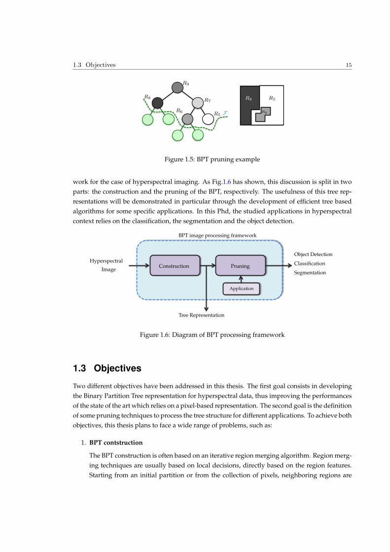
The tree processing of Fig.1.4 according to a specific application can be done by a pruning.
The pruning of the tree can be seen as a process aiming to remove subtrees composed of nodes
which are considered to be homogeneous with respect to some criterion of interest (homogeneity
criterion, e.g., intensity or texture). This task can be performed by analyzing a pruning criterion
along the tree branches to retrieve the nodes of largest area fulfilling the criterion. Given the
example of Fig.1.4 , a pruning example is shown in Fig.1.5 . The pruning is defined by the green
line which cuts the tree into two parts. In this case, the pruning strategy has removed the green
nodes corresponding to regions R1,R2,R3 and R4. The definition of this pruning gives us the
partition shown on the right of Fig.1.5. This partition has been obtained by selecting the leaf
nodes of the pruned tree. Note that Fig.1.5(b) only corresponds to one possible pruning result
from the BPT shown in Fig.1.4. Thus, different hyperspectral image processing aims can lead to
different pruning results. This can be understood as the BPT pruning is the application dependent
step regarding the BPT hyperspectral image processing framework.
The hyperspectral image processing framework based on BPT then relies on two steps illus-
trated in Fig.1.6. The first one corresponds to the construction of the BPT in the case of hyperspec-
tral data, enabling the exploitation of the spectral/spatial correlation. Accordingly, the second
step is a pruning strategy which is completely linked to a specific application.
The work developed in this thesis deals with the discussion of BPT image processing frame-
1.3 Objectives 15
R6R5
F
R7
R8
R9
R5
R6
R8
Figure 1.5: BPT pruning example
work for the case of hyperspectral imaging. As Fig.1.6 has shown, this discussion is split in two
parts: the construction and the pruning of the BPT, respectively. The usefulness of this tree rep-
resentations will be demonstrated in particular through the development of efficient tree based
algorithms for some specific applications. In this Phd, the studied applications in hyperspectral
context relies on the classification, the segmentation and the object detection.
!!
!! !!
!!
Construction Pruning
BPT image processing framework
Tree Representation
Application
Hyperspectral
ImageClassification
Segmentation
Object Detection
Figure 1.6: Diagram of BPT processing framework
1.3 Objectives
Two different objectives have been addressed in this thesis. The first goal consists in developing
the Binary Partition Tree representation for hyperspectral data, thus improving the performances
of the state of the art which relies on a pixel-based representation. The second goal is the definition
of some pruning techniques to process the tree structure for different applications. To achieve both
objectives, this thesis plans to face a wide range of problems, such as:
1. BPT contstruction
The BPT construction is often based on an iterative region merging algorithm. Region merg-
ing techniques are usually based on local decisions, directly based on the region features.
Starting from an initial partition or from the collection of pixels, neighboring regions are
16 Chapter 1. Introduction
iteratively merged. Thus, region merging algorithms are specified by: 1) a merging crite-
rion, defining the similarity between pair of neighboring regions; and 2) a region model that
determines how to represent a region and the union of two regions. Working with hyper-
spectral data, the definition of a region model and a merging criterion is not straighforward.
Thus, the study of both notions is going to be the first step in this PhD work.
• Region Model definition
In our case, the Region Model defines how to characterise a set of spectra forming an
hyperspectral region. The simplest solution is to use a first order model: the mean.
Hence, classical spectral distances between the mean of each region can be used as
merging criterion. Unfortunately, some limitations may come from the poor modeling
based on the mean. The first limitation comes from the fact that high intra-class spec-
tral variability can be found in an image region from the same material. The second
important issue is that, with the mean model, regions are assumed to be homogeneous.
This assumption is rarely true in natural scenes where textured regions are often ob-
served. Therefore, this PhD investigates alternative models which provides a general
strategy with less assumptions about the nature of the regions [17].
• Similarity Measure as Merging Criterion
Following the classical literature, the radiance values along all the wavebands should
be taken into account in order to discriminate two spectra. Consequently, the best clas-
sical distances between spectra are based on the overall shape of the reflectance curve
[16]. However, all the bands in the hyperspectral images are not equally important
in terms of discrimination. In particular, some materials can only be discriminated
in some hyperspectral bands of the spectral range. This issue is related to the strong
correlation existing between consecutive bands. Therefore, a good similarity metric
in the hyperspectral space should take into account the following issues: 1) the cor-
relation between bands in order to remove the redundant information and 2) a mul-
tivariate similarity measure taking into account the most important bands should be
established. During this PhD, similarity measures between hyperspectral regions will
be studied in order to define a good merging criterion for BPT construction.
2. BPT Pruning strategies
As mentioned before, the pruning strategy completely depends on the application of in-
terest. Accordingly, some pruning techniques will be proposed and discussed according
to different applications. We will focus in particular on segmentation, object detection and
classification of hyperspectral imagery.
• Classification application
The goal of this pruning is to remove subtrees composed of nodes belonging to the
same class. Thus, the final aim is to use the pruned BPT to construct a classification map
of the whole image. Note that using the pruned tree, the classification map describing

1.4 Thesis Organization 17
the pixel class assignment can be easily constructed by selecting the leaf nodes of the
resulting pruned tree. The method proposed here consists of two different steps. First,
some specific region descriptors are computed for each node. Then, the second step
involves a BPT analysis to take the pruning decision.
• Segmentation application
The segmentation pruning consists in extracting from BPT a partition of hyperspectral
image where the most meaningful regions are formed. Thus, the goal of such appli-
cation is to remove subtrees which can be replaced by a single node. All the nodes
inside a subtree can be replaced if they belong to the same region in the image space.
This means that the distance between them is small and the distance between them
and their BPT neighboring nodes is high.
In this context, two different approaches are studied in this thesis. Firstly, the hyper-
spectral segmentation goal is tackled by a global energy minimization strategy. This
approach defines an error associated to each partition contained in the BPT and then,
it extracts the partition having the minimum error. The second approach focused on
hyperspectral image segmentation is based on applying normalized cuts on the BPT
branches. The purpose of this second approach is to study how the classical spectral
graph partitioning technique can be applied on BPT structures.
• Object Detection application
The BPT is studied here as a new scale-space of the image representation in the con-
text of hyperspectral object detection. The recognition of the reference objects in hy-
perspectral images has been mainly focused on detecting isolated pixels with similar
spectral characteristics. In contrast, this thesis presents the BPT hyperspectral image
representation in order to perform a different object detection strategy. To this goal, the
detection of two specific reference objects from an urban scene is investigated. Hence,
the methodology to extract BPT nodes forming these objects is studied.
1.4 Thesis Organization
This thesis proposes the construction and the processing of BPT image representation in the case
of hyperspectral images. The major goals are, on the one hand, to develop the construction of
BPT region-based representation and, on the other hand, to propose some pruning strategies
according to three different applications. To tackle these points, this PhD dissertation is divided
into five major parts:
1. In this first chapter, the context of this thesis is introduced. After briefly presenting hyper-
spectral imagery and, the Binary Partition Tree representation, the objectives and the thesis
organization are described.
2. The second chapter provides the background for hyperspectral image processing and hi-
erarchical tree representations. The basic terms used in this Phd are introduced and the

18 Chapter 1. Introduction
techniques proposed in the state of the art are reviewed.
3. In the third chapter, the BPT construction for hyperspectral images is investigated. Different
merging orders are defined by combining different region models and merging criteria. The
different merging orders result in different BPT constructions. Thus, some experiments are
carried out in order to analyze the various constructed BPTs. The quantitative validation of
the BPT construction has been performed based on different manually created ground truth
data. Also in this chapter, a comparison against the classical state of the art technique that
is typically used for hierarchical hyperspectral image segmentation is presented.
4. Different BPT pruning strategies are examined in the fourth chapter. The different appli-
cations and their corresponding pruning strategies are presented in the different sections.
First, a supervised classification of hyperpectral data is described. Afterward, two different
sections tackle the supervised and unsupervised image segmentation goals by perform-
ing two different approaches. A strategy based on energy minimization is firstly proposed
based on a constrained lagrangian function. This approach is supervised because the num-
ber of regions that wants to be obtained at the partition result is previously known. Con-
cerning the unsupervised approach, this chapter presents a pruning strategy based on nor-
malized cut and spectral graph partitioning theory.
Finally, this chapter introduces a hyperspectral object detection procedure using BPT image
representation. Two different examples are described respectively detailing the recognition
of roads and buildings in urban scenes. Each of the aforementioned parts describing the
different application begins with a short introduction to the problems to be addressed. Be-
sides, experimental results are reported on various real data sets according to the distinct
application goals.These results are conducted to assess and validate the interest of the pro-
posed algorithms. Furthermore, each of these sections present the main conclusions of the
approach as well as future perspective.
5. The last chapter summarizes the main points discussed along the thesis and highlights the
major conclusions.
This thesis is concluded by a series of appendices describing different aspects related to the
topics discussed along this work. First, the characteristic of tree performances are discussed.
Then, the acronyms used in this PhD dissertation and a mathematical appendix is presented.
Finally, more results and the list of publications are included.
2State of the art
Contents
2.1 Hyperspectral image processing . . . . . . . . . . . . . . . . . . . . . . . . . . . . 20
2.1.1 Classification techniques incorporating spatial constraints . . . . . . . . . . 21
2.1.2 Traditional imagery techniques extended to HSI . . . . . . . . . . . . . . . 25
2.2 Hierarchical region-based processing using trees . . . . . . . . . . . . . . . . . . . 33
2.2.1 Definition of the tree structure . . . . . . . . . . . . . . . . . . . . . . . . . . 35
2.2.2 First hierarchical tree representations . . . . . . . . . . . . . . . . . . . . . . 36
2.2.3 BPT Literature . . . . . . . . . . . . . . . . . . . . . . . . . . . . . . . . . . . 38
2.3 Conclusions . . . . . . . . . . . . . . . . . . . . . . . . . . . . . . . . . . . . . . . . 39
This chapter provides the background for hyperspectral image processing and hierarchical
tree region-based representations. The first section details the hyperspectral image analysis state
of the art, stressing the importance of the spectral-spatial hyperspectral information. The second
section explains the interest of studying hierarchical region-based representations, and also the
importance of using tree-based structures. The basic terms and the current state of the art of tree
image representations are detailed, justifying the choice of the Binary Partition Tree. Finally, a
review of the BPT related literature is presented.
20 Chapter 2. State of the art
2.1 Hyperspectral image processing
Particular attention has been paid in the literature to hyperspectral image processing in the last
ten years. A large number of techniques have been proposed to process hyperspectral data. As a
matter of fact, the processing of such images not straightforward [72].
The first important drawback is the high dimensionality of the space which contains a lot of re-
dundant information and requires a tremendous computational effort. In order to manage it,
an important number of hyperspectral techniques have focused on transforming the data into
a lower dimensional subspace without losing significant information in terms of separability
among the different materials. In this context, several supervised and unsupervised dimension
reduction techniques have been proposed for hyperspectral imaging.
Based on image statistics, Principal Component Analysis (PCA) and Independent Component
Analysis (ICA) [74] are the two most used unsupervised techniques. Regarding supervised tech-
niques, some examples are the Discriminant Analysis Feature Extraction (DAFE)[75], Decision
Boundary Feature Extraction (DBFE), and Non-parametric Weighted Feature Extraction (NWFE)
[76][77]. These supervised methods reduce the high dimensionality by minimizing a classifica-
tion criterion by using some ground truth data.
The second important challenge in hyperspectral image techniques corresponds to the processing
of the data in a joint spectral-spatial space. Early analysis techniques are traditionally focused on
the spectral properties of the hyperspectral data using only the spectral space. These pixel-based
procedures analyze the spectral properties of each pixel, without taking the spatial or contex-
tual information related to the pixel of interest into account. Thus, these techniques are quite
sensitive to noise and lack of robustness. In this framework, many different supervised and semi-
supervised techniques have been proposed to perform pixelwise classification [2],[3],[4],[5],[6].
Without taking the spatial location of the pixels into consideration (i.e: only studying spectral
proprerties), these techniques assign to each pixel the label corresponding to its predicted class.
In the last few years, the importance of the spatial space and, in particular, of taking into account
the spatial correlation has been demonstrated in different contexts such as classification [10] [?],
image segmentation [11] [12] [13] or unmixing [8]. With this approach, hyperspectral images are
viewed as arrays of ordered pixel spectra which enables to combine the spatial and the spectral
information. For instance, in a classification context, pixels are classified according to the spectral
information and according to the information provided by their spatial neighborhood.
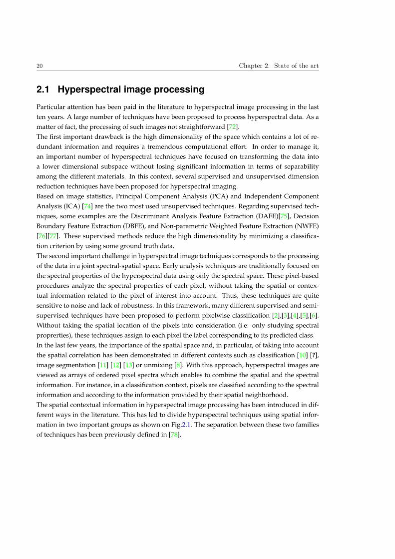
The spatial contextual information in hyperspectral image processing has been introduced in dif-
ferent ways in the literature. This has led to divide hyperspectral techniques using spatial infor-
mation in two important groups as shown on Fig.2.1. The separation between these two families
of techniques has been previously defined in [78].
2.1 Hyperspectral image processing 21
Spectral-based
classification
incorporating
spatial constraints
Extension of classical
image processing
techniques to HSI
Spectral-Spatial methods
Figure 2.1: Spectral-Spatial Hyperspectral processing techniques
1. Classification with spatial constraints: This family of techniques corresponds to all the super-
vised and unsupervised classification methods incorporating spatial constraints.
2. Extension of classical techniques to HSI: This second group of hyperspectral methods is formed
by all the techniques which are the extension of classical image processing techniques to
high dimensional spaces.
According to this classification, the aim of the next subsections is to review some of the tech-
niques related to each category. In 2.1.1, different methodologies introducing the spatial informa-
tion in different stages of the classification process are presented. The other category of techniques
is reviewed in 2.1.2. It deals with methods involving the extension of some classical image pro-
cessing tools to hyperspectral imaging.
2.1.1 Classification techniques incorporating spatial constraints
Classification is one of the most studied applications in hyperspectral imagery. The goal is to
label each pixel with the label corresponding to the class or the object that it belongs to. In the
literature, the best classification results have been obtained by techniques incorporating the spa-
tial information to the spectral space. The incorporation of the spatial or contextual information
improves pixel-wise classification results which usually present an important salt and pepper noise
(misclassification of individual pixels).
Thus, it seems clear that spatial knowledge should be incorporated during the classification
methodology, the main question is then at which stage and how it should be included.
• Is it better to incorporate spatial information as an input data before classifying the data?
• Should the spatial information be included in the classification decision?
• Is the incorporation of the spatial information a post-processing stage of the classification
process?
22 Chapter 2. State of the art
The incorporation of the spatial information has been suggested in different manners. This
work reviews three groups of techniques according to these three discussed questions.
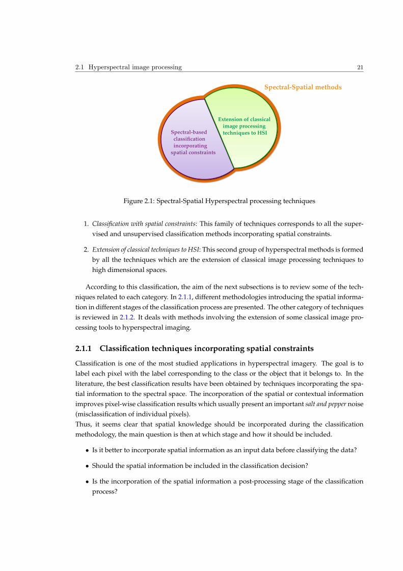
Spatial information as an input parameter
Some methods include the use of the spatial domain in an early stage. These techniques are
characterized by computing in a first step some spatial image measurements which are later used
by a classifier. The flowchart describing this approach is shown in Fig.2.2
Hyperspectral
Image
Classification MapSpatial information
Classification Framework
Classification
Figure 2.2: Spatial information as an input parameter
In some strategies following this scheme, this first step consists in constructing a spectral and
spatial feature vector for each pixel which is later used as an input parameter in a pixel-wise clas-
sication task. An example is found in [79] , where the Gray Level Co-occurrence Matrix (GLCM)
image measurements (Angular Second Moment, Contrast, Entropy and Homogeneity) are com-
puted as a first step. These four texture measurements form a set of images which is decomposed
by a Principal Component Analysis (PCA) to obtain its Principal Components (PCs). This last
information is then used as an input feature for a Maximum Likelihood classifier.
Using another image reduction technique such as the Non-negative Matrix Factorization MNF,
these GLCM texture measurements were also studied in [80]. They are used jointly with some
spectral features to propose a supervised classification using the well-known Support Vector Ma-
chine (SVM) classifier.
Other strategies try to classify hyperspectral data by using a segmentation map as an input pa-
rameter. These approaches start by partitioning the image into homogeneous regions and then
classifying each region as a single object. Most of these methods are based on the work presented
in [81] which is the first standard approach proposed to join spectral and spatial domain in mul-
tispectral imagery. It corresponds to the ECHO (Extraction and Classification of Homogeneous
Objects) classifier. In this method, an image is segmented into statistically homogeneous regions
by the following recursive partitioning algorithm:
• First, an image is divided by a rectangular grid into small regions, each region containing
an initial number of pixels.
• Then, following an iterative algorithm, an homogeneity criterion is tested between adjacent
regions. If the test does not fail, these regions are merged forming a new region which will
2.1 Hyperspectral image processing 23
be evaluated in the next iteration. In the other case, the minimal required homogeneity is
not achieved, the region is then classified by using a ML classifier.
A recent work in [87] has extended this algorithm to an unsupervised version, where an image is
also divided into different homogeneous regions according to their spatial-spectral similarities.
The classical ECHO classification methodology has also been followed in [82]. This technique
proposes as a first step the extraction of some image features to reduce the image dimension.
A merging algorithm similar to ECHO is then applied on the reduced image to construct a parti-
tion. Then, a SVM classifier is used to classify each region of the partition map. The SVM classifier
has largely demonstrated its effectiveness in hyperspectral data. Thus, it has been also used in
[83]. This work defines a neighborhood by using a segmentation result before applying a SVM
classifier for every region. The segmentation map is obtained by a region growing segmentation
performed by the eCognition software[84].
In the context of hyperspectral classification, a study of the pixel neighborhood definition to be
used with SVM classifier can be found in [85] , where techniques as watershed [86] and Recursive
hierarchical segmentation software [?] have been studied. In these last techniques, the classifi-
cation map plays a different role in the classification decision. Instead of classifying a partition
region by considering its spectral mean values, a majority voting decision is studied within the
classification map regions.
One of the most critical aspects for the methods using partition maps as an input parameter is that
they are very sensitive to the initial segmentation settings. For instance, the number of regions
and the regions edges from the spatial partition of the image are critical parameters to achieve a
good classification in the later step.
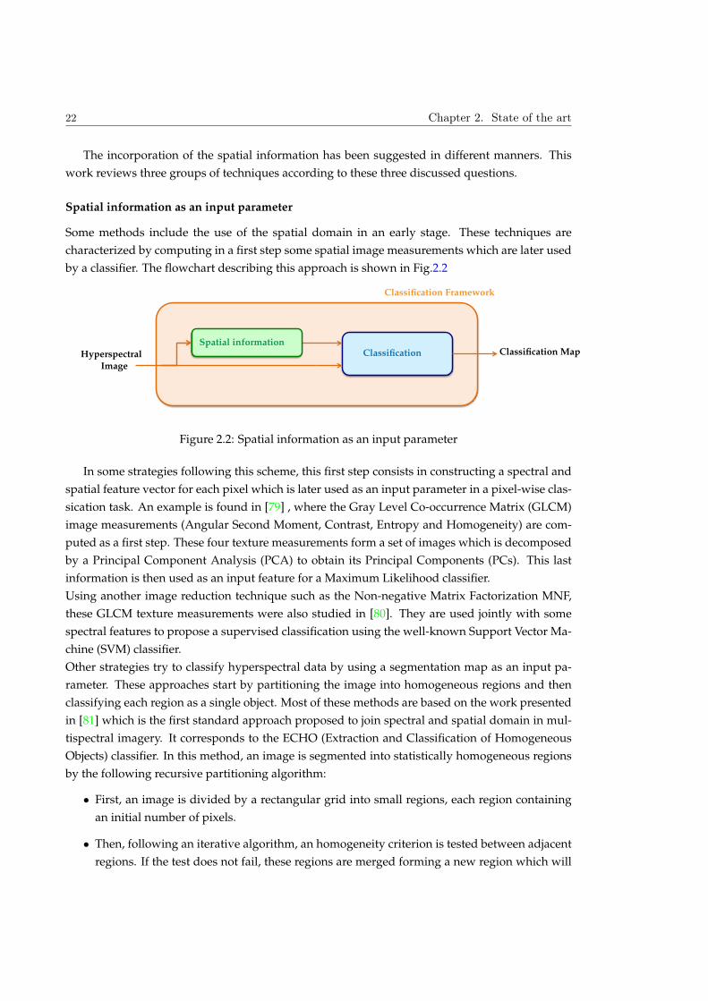
Spatial information inside the classification decision
The second important group of spatial-spectral classification techniques have considered that the
spatial information should be included in the classification decision rule. Fig.2.3 describes the
framework of this methodology.
Hyperspectral
Image Classification Map
Spatial information
Classification Framework
Spectral/Spatial
Classification
Figure 2.3: Spatial information inside the classification decision
Following this strategy, some methods have proposed to introduce the spatial constraints in-
side the SVM classifier decision. The approach of such methods proposed by [88] consists in

24 Chapter 2. State of the art
introducing the spatial information through the kernel functions. It has been demonstrated in
[88] that any linear combination of kernels actually is a kernel K = K1 + K2: if K1 and K2 are
two kernels functions fulfilling Mercer’s conditions [88]. The interest is then to construct a com-
bination of spatial and spectral kernel as K(x, y) = µKspectral(x, y) + (1 − µ)Kspatial(x, y) where
µ weights the relative importance of the spectral and spatial information.
The work presented in [88] proposes a gaussian kernel as Kspectral by using the euclidean dis-
tance. Concerning the contextual information, Kspatial introduces information about the local
mean and variance for each pixel using a fixed square neighborhood. As mentioned by the
authors, some problems can be found in this spatial kernel because of the fixed neighborhood
window. In order to overcome the phenomena of edge effect (misclassifications in the transi-
tion zones), the method presented in [89] proposes an adaptive spatial neighborhood for Kspatial.
Morphological filters are used to extract the connected components of the image which are as-
signed to each pixel as its adaptive neighborhood. The vector median value is computed for each
connected component and this value is then used as the contextual feature for Kspatial.
Other approaches, not using SVM classifier, also include spatial information in the classification
decision. For instance, in [91] and [90], authors have proposed unsupervised and supervised
classification by estimating the class probability of each pixel through a defined spatial-spectral
similarity function. Concerning the spectral decision, the Spectral Angle Mapper (SAM) is used
as a discriminative measure showing its effectiveness in [92] . Concerning spatial discrimination,
a stochastic watershed algorithm is proposed for segmenting hyperspectral data.
Spatial information as a post-processing stage
The third and last familiy of hyperspectral classification techniques reviewed here performs a
post-processing in order to incorporate the spatial information. This regularization step avoids
possible errors obtained by classification methods using only the spectral information. The fol-
lowed methodology is represented by Fig.2.4.
Hyperspectral
Image Classification MapSpatial
Regularization
Classification Framework
Spectral
Classification
Figure 2.4: Spatial information as a post-processing stage
An important number of techniques are characterized by proposing the Markov Random Field
MRF model [93] as the spatial post-processing task. The methodology of such approaches relies
on three different steps. Firstly, hyperspectral data are classified in order to assign to each pixel its
class-conditional PDFs. Secondly, using the classification results, an energy function composed
2.1 Hyperspectral image processing 25
by one spectral and one spatial term is defined. For this energy function, the spectral energy term
is usually derived from its class-conditional probability whereas the spatial energy term is com-
puted by evaluating the class-probability of the neighborhood. Finally, the last step consists in
labeling each hypespectral pixel with one class. This is done by the minimization of the energy
function which has been formulated as a maximum a posteriori (MAP) decision rule.
In hyperspectral literature, different classifiers have been used for assigning class-conditional
PDFs before constructing an energy function. In [96] , a DAFE dimension reduction used by a
Bayesian classifier has been proposed. Another class-Pdfs estimation is proposed in [94] where
the pixelwise ML classifier is used. The integration of the SVM technique within a MRF frame-
work has been used in [100] [98] [99]. Also, in [97] class-conditional PDFs are estimated by the
Mean Field-based SVM regression algorithm. Recent works have proposed to estimate the poste-
rior probability distributions by a multinomial logistic regression model[101] [102]. For instance,
the method presented in [101] first proposes a class-PDFs estimation by using a MLR classifica-
tion step and then a MAP classification by minimizing the energy function using the ↵-Expansion
min-cut algorithm.
Besides of these studies, some other works have been proposed in the literature involving hyper-
spectral image processing by MRF (See [78]).
2.1.2 Traditional imagery techniques extended to HSI
Traditional imagery techniques commonly used to process gray-scale, RGB or multispectral im-
ages are not suited to the dimensionality of the data present in a hyperspectral image. In order
to address the high dimensionality issue, two different approaches have been mainly suggested.
One solution consists in reducing considerably the hyperspectral data dimension in order to work
with classical techniques. The other procedure is based on the extension of certain operations or
image processing fundamentals into this new multi-dimensionality.
Following both approaches, classical techniques such as morphological filters, watershed trans-
formations, hierarchical segmentation, diffusion filtering or scale-space representation, have been
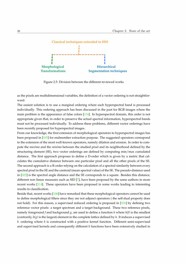
extended for HSI imaging. Within this large group of algorithms, this section will focus on two
groups: the morphological transformations and the hierarchical segmentation techniques (See
Fig.2.5). In order to increase the knowledge about the extension of other classical techniques, a
review of diffusion filtering techniques is presented in [78].
Transformations based on Mathematical Morphology
The first group of techniques reviewed here are the works concerning mathematical morphology
transformations. In traditional imagery, the importance of mathematical morphology has grown
and it has become a popular and solid theory over the past decades [103]. This nonlinear method-
ology has lead to the definition of a wide range of image processing operators. Based on lattice
theory, the morphological operator are based on maxima and minima operations. This implies the
definition of an ordering relation between the image pixels. In the case of hyperspectral image,
26 Chapter 2. State of the art
Hierarchical
Segmentation techniques
Classical techniques extended to HSI
Morphological
Transformations
Figure 2.5: Division between the different reviewed works
as the pixels are multidimensional variables, the definition of a vector ordering is not straightfor-
ward.
The easiest solution is to use a marginal ordering where each hyperspectral band is processed
individually. This ordering approach has been discussed in the past for RGB images where the
main problem is the appearance of false colors [104]. In hyperspectral domain, this order is not
appropriate given that, in order to preserve the actual spectral information, hyperspectral bands
must not be processed individually. To address these problems, different vector orderings have
been recently proposed for hyperspectral images.
From our knowledge, the first extension of morphological operators to hyperspectral images has
been proposed in [105] for endmember extraction purpose. The suggested operators correspond
to the extension of the most well-known operators, namely dilation and erosion. In order to com-
pute the maxima and the minima between the studied pixel and its neighborhood defined by the
structuring element (SE), two vector orderings are defined by computing min/max cumulated
distance. The first approach proposes to define a D-order which is given by a metric that cal-
culates the cumulative distance between one particular pixel and all the other pixels of the SE.
The second approach is a R-order relying on the calculation of a spectral similarity between every
spectral pixel in the SE and the centroid (mean spectral value) of the SE. The pseudo-distance used
in [105] is the spectral angle distance and the SE corresponds to a square. Besides this distance,
different non linear measures such as SID [7], have been proposed by the same authors in more
recent works [114]. These operators have been proposed in some works leading to interesting
results in classification.
Beside that, recent works [106] have remarked that these morphological operators cannot be used
to define morphological filters since they are not adjunct operators ( the self-dual property does
not hold). For this reason, a supervised reduced ordering is proposed in [106] by defining two
reference vector pixels: a target spectrum and a target background. These two reference pixels,
namely foreground f and background g, are used to define a function h where h(f) is the smallest
(contrarily, h(g) is the largest) element in the complete lattice defined by h. It induces a supervised
h -ordering where h is constructed with a positive kernel function. Different semi-supervised
and supervised kernels and consequently different h functions have been extensively studied in
2.1 Hyperspectral image processing 27
[107]. The definition of the h-ordering has allowed authors to define different morphological op-
erators such as the top-hat transformation which extracts contrasted components with respect to
the background.
Other well-known operators of mathematical morphology are morphological profiles MPs [108].
These operators are computed by successively applying classical geodesic opening and closing
operations. At each operation, the structuring element size is increased gradually. These oper-
ators have been studied in HSI in several works mostly focusing on data classification. Most of
these studies have addressed the huge dimensionality issue by first reducing the hyperspectral
image dimension. Hence, hyperspectral dimension reduction techniques are usually proposed as
a first step before constructing MPs.
One of the first work introducing these operators for HSI images can be found in [109] where
PCA is proposed as a first step to reduce the hyperspectral image dimension. The first principal
component band, describing the maximum data variance direction, is then used as a gray scale
image for computing classical MPs.
Following this approach, the work in [110] has also proposed the use of the gray scale first princi-
pal component image for constructing MPs. The resulting MPs are used here to classify the data
by using the fuzzy ARTMAP method.
These two last works have only considered a single band image from PCA to perform Morpho-
logical Profiles. Consequently, the dimensionality reduction applied for these techniques can lead
to a significant loss of information. To manage this issue, Extended Morphological Profiles EMP
have been proposed in [111]. In this work, PCA technique is also proposed to reduce the image
dimensionality. However, more components are taken to form the reduced space. The number of
components is given by comparing the total cumulated variance of the data associated to the PCs
with a threshold usually set to 99%. The resulting PCs are used to build individual morphological
profiles (one for each PC), which are combined together in one extended morphological profile.
In [111], EMPs are then single stacked vectors which are classified with a neural network, with
and without feature extraction.
Another classification works [89] has further investigated the EMP construction for applying SVM
classification. Concerning the image reduction technique, some techniques have considered ICA
instead of PCA for computing the EMP [112]. Instead of the conventional PCA, a Kernel Principal
Component Analysis is proposed in [115] as supervised feature reduction technique for comput-
ing the EMP.
Although most techniques have proposed to reduce the dimensionality of the image, the work
presented in [114] has proposed the MPs construction by using the full spectral information. Us-
ing the morphological operators defined in [105] , the authors proposed in [114] different morpho-
logical profiles without any dimensionality reduction stage. In a SVM classification background,
this new multi-channel MPs are compared with MPs computed in a reduced space.
The extraction of spatial features from hyperspectral images by using MPs or EMPs have shown
their good performances in a large number of applications as classification or unmixing. How-
ever, these transformations cannot fully provide the spatial information of an image scene. This is
28 Chapter 2. State of the art
because they are based on morphological geodesic opening and closing filters which only act on
the extrema of the image. Consequently, MPs only provide a partial analysis of the spatial infor-
mation analyzing the interaction of a set of SEs of fixed shape and increasing size with the image
objects. In order to solve these limitations, morphological attribute filters have been proposed in-
stead of the conventional geodesic operators to construct Extended Attribute Profiles EAPs[113].
The application of attribute filters in a multilevel way leads to describe the image by other fea-
tures such as shape, texture or homogeneity. EAPs have been also proposed for hyperspectral
data classification and they have been constructed after applying different dimensionality reduc-
tion techniques such as PCA or ICA[113].
As can be seen, most of the techniques concerning MP, EMP or EAP are focused on hyperspectral
classification. Thus, they could be also included in the first group of classification techniques re-
viewed in Sec.2.1.1. In fact, these morphological operators have been used to estimate in different
manners the spatial information which is lately used in a classification stage.
Going on with morphological operators, another important algorithm extended to hyperspectral
image is the watershed. This transformation is based on considering each frequency band im-
age as a topographic relief, whose elevation depends on the pixel values. In this topographic
relief, the local minima are considered as catchment basins. In the first step, some image minima
are defined as markers which are the sources of the catchment basins. Then, a flooding process
of the catchment basins is performed by a region growing step starting from each marker. The
flooding process finalizes when two different catchment basins meet, hence defining a watershed
line(edge). The resulting image partition of watershed algorithm is obtained by these edges.
In the case of color image, the classical watershed algorithm is computed by interpreting the
height of the image color gradient as the elevation information. Thus, the extension of watershed
algorithm to HSI relies on defining how to extract the gradient in the multidimensional space.
One of the first works involving watershed in HSI data can be found in [116]. In this study, dif-
ferent gradient functions have been proposed to construct a stochastic watershed algorithm. The
aim of stochastic watershed is to define an algorithm that is relatively independent of the markers
by introducing a probability density function of contours. This pdf gives the edge strength which
can be interpreted as the probability of pixels of belonging to the segmentation contour. The pdf
of contours can be estimated by assigning to each pixel the number of times that it appears as
an edge in a series of segmentations. In the hyperspectral case, the construction of such pdf has
been studied taking into account all the hyperspectral bands or only using some of them after a
dimensionality reduction [116]. In this last work, the contour pdf function is used to construct
watershed algorithm in two different manners. The first approach consists in using the contour
pdf function instead of the classical color gradient. The second approach is to used the contour
pdf to construct a new probabilistic gradient based on the sum of the color gradient and the con-
tour pdf.
Following the first strategy, a vector approach has been proposed where the pdf is computed by
a similarity distance taking into account all the bands (with or without reduction). A marginal
approach has also been proposed by computing one marginal pdf for each channel. The resulting
2.1 Hyperspectral image processing 29
pdf is then defined by a linear weighted combination of all marginal pdfs (the weights are for
example the inertia axes ).
The second approach consists in performing watershed algorithm by using a probabilistic gra-
dient based on the sum of color gradient and the contour pdf. The strategy of constructing a
probabilistic gradient has been pursued in recent works [91] for hyperpsectral image segmenta-
tion. In this case, the proposed gradient is also a sum between a gradient distance and a pdf
contour function. However, some new pdf contour estimators are proposed using different mul-
tiscale segmentations and introducing spectral information.
Besides stochastic watershed, other color gradient functions (without introducing pdfs of con-
tours) have been proposed for hyperspectral classification. In [85] , robust color morphological
gradient and color morphological gradient have been proposed to perform the watershed algo-
rithm. These gradient functions have been performed after reducing the dimensionality of the
hyperspectral image. The result of the watershed algorithm has been used to define an image
adaptive neighborhood for a SVM classification purpose.
Hierarchical segmentation techniques
Image segmentation is interpreted as an exhaustive partitioning of an image. Each region is con-
sidered to be homogeneous with respect to some criterion of interest. The aim of segmentation is
the extraction of image regions as primary visual components that can be used later to identify
and recognize objects of interest. The main problem is that it is very difficult to directly construct
the best image partition (if there is any) given the huge number of applications potentially con-
sidered for one given image.
Let us consider for instance a high-resolution aerial image which is formed by an urban and a
vegetation areas. Working at coarse scales, some applications can be defined to separate between
fields and cities. However, applications focusing on individual tree or building detection should
work for the same image at a much lower scale.
The interpretation of an image at different scales of analysis has led some authors to deal with
multi-scale image segmentations. A multi-scale image segmentation relies on the construction of
hierarchy of partitions mainly based on an iterative region merging algorithm ( See Def.3). The
result of the hierarchical segmentation technique is then an image partition representing a hierar-
chical level obtained after a region merging procedure.
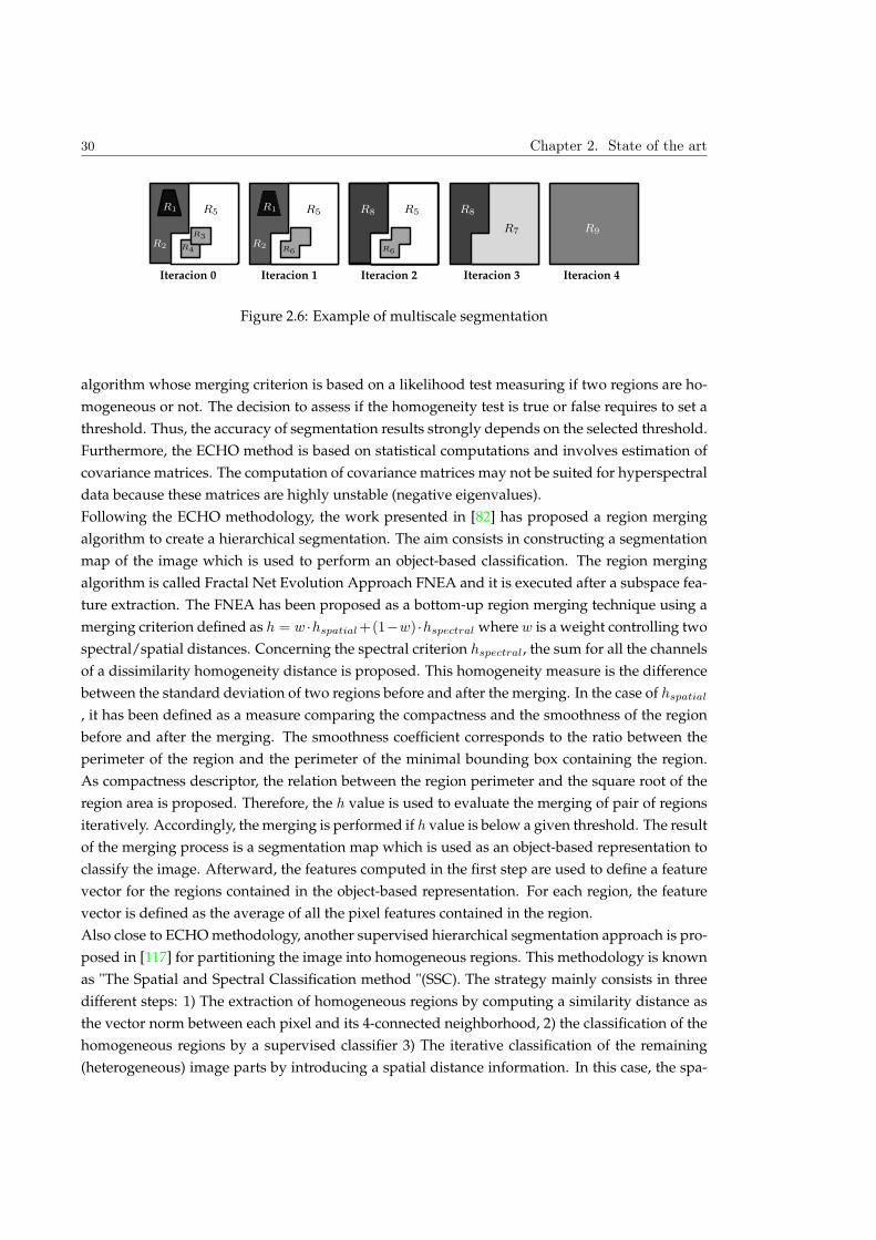
Fig.2.6 shows an example of multi-scale segmentation where a region merging algorithm has
been performed on the image Iteration 0. The partitions created during the iterative procedure are
shown consecutively from the left to the right. Note that once these five hierarchical partitions
are computed, a criterion related to the addressed application is needed in order to select the ap-
propriate level of the hierarchy. Consequently, the segmentation result obtained for this example
will be one of the following partitions: Iteration 0, Iteration 1, Iteration 2, Iteration 3 or Iteration 4.
Hierarchical segmentation techniques have been also studied for hyperspectral data. Some
of them are mentioned in Section2.1.1. In this framework, ECHO was the first proposed hierar-
chical segmentation technique [81]. As previously explained, ECHO proposes a region merging
30 Chapter 2. State of the art
R1
R2
R1 R8
R2
R3
R4 R6 R6
R5 R5 R5
R7
R8
R9
Iteracion 4Iteracion 3Iteracion 2Iteracion 1Iteracion 0
Figure 2.6: Example of multiscale segmentation
algorithm whose merging criterion is based on a likelihood test measuring if two regions are ho-
mogeneous or not. The decision to assess if the homogeneity test is true or false requires to set a
threshold. Thus, the accuracy of segmentation results strongly depends on the selected threshold.
Furthermore, the ECHO method is based on statistical computations and involves estimation of
covariance matrices. The computation of covariance matrices may not be suited for hyperspectral
data because these matrices are highly unstable (negative eigenvalues).
Following the ECHO methodology, the work presented in [82] has proposed a region merging
algorithm to create a hierarchical segmentation. The aim consists in constructing a segmentation
map of the image which is used to perform an object-based classification. The region merging
algorithm is called Fractal Net Evolution Approach FNEA and it is executed after a subspace fea-
ture extraction. The FNEA has been proposed as a bottom-up region merging technique using a
merging criterion defined as h = w ·hspatial+(1−w) ·hspectral where w is a weight controlling two
spectral/spatial distances. Concerning the spectral criterion hspectral, the sum for all the channels
of a dissimilarity homogeneity distance is proposed. This homogeneity measure is the difference
between the standard deviation of two regions before and after the merging. In the case of hspatial
, it has been defined as a measure comparing the compactness and the smoothness of the region
before and after the merging. The smoothness coefficient corresponds to the ratio between the
perimeter of the region and the perimeter of the minimal bounding box containing the region.
As compactness descriptor, the relation between the region perimeter and the square root of the
region area is proposed. Therefore, the h value is used to evaluate the merging of pair of regions
iteratively. Accordingly, the merging is performed if h value is below a given threshold. The result
of the merging process is a segmentation map which is used as an object-based representation to
classify the image. Afterward, the features computed in the first step are used to define a feature
vector for the regions contained in the object-based representation. For each region, the feature
vector is defined as the average of all the pixel features contained in the region.
Also close to ECHO methodology, another supervised hierarchical segmentation approach is pro-
posed in [117] for partitioning the image into homogeneous regions. This methodology is known
as "The Spatial and Spectral Classification method "(SSC). The strategy mainly consists in three
different steps: 1) The extraction of homogeneous regions by computing a similarity distance as
the vector norm between each pixel and its 4-connected neighborhood, 2) the classification of the
homogeneous regions by a supervised classifier 3) The iterative classification of the remaining
(heterogeneous) image parts by introducing a spatial distance information. In this case, the spa-
2.1 Hyperspectral image processing 31
tial distance provides information about the class of the neighboring pixels around the studied
pixel.
One of the most well-known hierarchical segmentation methods in hyperspectral data can be
found in [120] . The proposed algorithm is based on the hierarchical sequential optimization al-
gorithm (HSWO for Optimal Hierarchical step-Wise Segmentation) [119] and it has been adapted
to hyperspectral data [22]. It relies on three steps:
1. Using the pixel-based representation of an image, a region label is assigned to each pixel (if
there is no pre-segmentation step).
2. A dissimilarity criterion is computed between all pairs of adjacent regions. The fusion of
two adjacent regions is performed if the distance is below a minimum threshold.
3. The algorithm stops if there is no more possible merging steps, otherwise it returns to step
2.
For the second step, the dissimilarity vector norm, the spectral information divergence SID,
the spectral angle mapper SAM or the normalized vector distance NVD have been proposed.
Recently, in order to mitigate the important computational cost of the initial approach, an algo-
rithm called recursive approximation RHSEG ("Recursive Hierarchical Segmentation") has been
proposed [121]. It has been recently used in a classification context [?].
Another generic hierarchical segmentation is presented in [78] based on an iterative process and a
cross analysis of spectral and spatial information.The hierarchical segmentation algorithm is im-
plemented by using a split and merge strategy. First, the image is over-segmented by a series of
splits based on spectral and spatial features following a strategy called butterfly. Secondly, setting
a stopping criterion, as for instance the number of regions, a region merging procedure based on
split and merge operations is performed until the stopping criterion is fulfilled. The construction
of a split and merge operations is carried out by the diagonalization of the matrices describing
the intra- and inter-region variance,respectively.
The general conclusion of this review on hierarchical segmentation for hyperspectral data is that
these techniques perform an iterative region merging algorithm based on certain similarity cri-
teria, until the predefined termination criterion is achieved. One of the main problems of such
strategy is that they assume that the "best" partition corresponds to one hierarchical segmenta-
tion level. Unfortunately, this assumption is rarely true and it can lead to some issues when the
coherent objects are found at different levels of the hierarchy.
For instance, assume that for the hierarchical segmentation of Fig.2.6 the optimal partition from a
given segmentation goal is formed by R7 and R8. It can be noticed that in this case, the optimal
partition is contained in the hierarchy at level corresponding to iteration 3. However, it should be
also remarked that an application looking for an optimal partition formed by R7, R1 and R2 will
never reach its purposes. This is because a large amount of information is lost in the hierarchical
segmentation techniques. They actually provide a rather limited number of partitions. This also
shows that these multiscale segmentations are not generic representations, in the sense that they
32 Chapter 2. State of the art
cannot be further processed according to different applications. The processing of a hierarchical
representation can offer various advantages as compared to the strategy of creating a segmenta-
tion map following a region merging procedure. For this reason, some recent works try to process
results contained in the hierarchy [122], [118] .
The work presented in [118] has proposed an example of processing hierarchical segmentation to
find coherent objects in the image. In order to process the partition hierarchy, segmentation results
are represented by a tree structure. In a first step, this work constructs a hierarchical segmenta-
tion of the image after reducing the dimensionality of the image performing a PCA reduction.
The hierarchical segmentation is performed by constructing an opening and closing profile [108].
It is carried out by applying morphological operators on each individual spectral bands using SE
of increasing sizes. These granulometry series produce a set of connected components forming a
hierarchy of segments in each band. Each pixel can then be assigned to more than one connected
component at each SE scale. The aim of constructing such a hierarchy is to look for connected
components which correspond to objects. To this end, authors have then proposed to structure
the hierarchical segmentation by a tree representation where each connected component is a node.
Concerning the edges of the tree, they represent the link between two consecutive scales of the
hierarchy. Thus, the edges correspond to the inclusion relationship where each node is inher-
ently contained in its parent node. In this case, the processing of a tree representing hyperspectral
data has started showing the advantages of hierarchical representations by using trees. Given the
object detection goal, the tree is used to select homogeneous regions contained in the nodes by
using the standard deviation of the spectral information of each region. The proposed criterion
corresponds to the difference between standard deviation of a node and its descendants.
Besides this last work, in parallel of this thesis, another tree image representation has been stud-
ied for processing hyperspectral images. This representation is the max-min tree [135] which has
been studied in hyperspectral context in [113] (See Fig.Fig.2.11). Working in a reduced PCA hy-
perspectral space, this work shows another important benefit of tree structures: their scalability.
This property allows to compute region descripors on the nodes to perform EAP by using the
inclusion hierarchy of the tree. As mentioned before, these morphological transformations, that
can be easily defined using tree, have corroborated their performances in hyperspectral image
classification.
Both hyperspectral tree image representations proposed in [113] and [118] are based on morpho-
logical construction tools. Therefore, the segmentation results stored in the hierarchy corresponds
to the connected components associated to a merging order performed by granulometry series.
Merging orders constructed by an iterative morphological filtering have some difference with re-
gion merging segmentation algorithms. The work in [123] has shown how the merging order
constructed by iterative morphological filters does not efficiently represent objects as a connected
components.
Given a one-band image, by using region merging segmentation algorithm, objects correspond to
connected components that are homogeneous in their gray level. Thus, the merging criterion of
these techniques consists in a measure evaluating this homogeneity notion. Instead, in the case
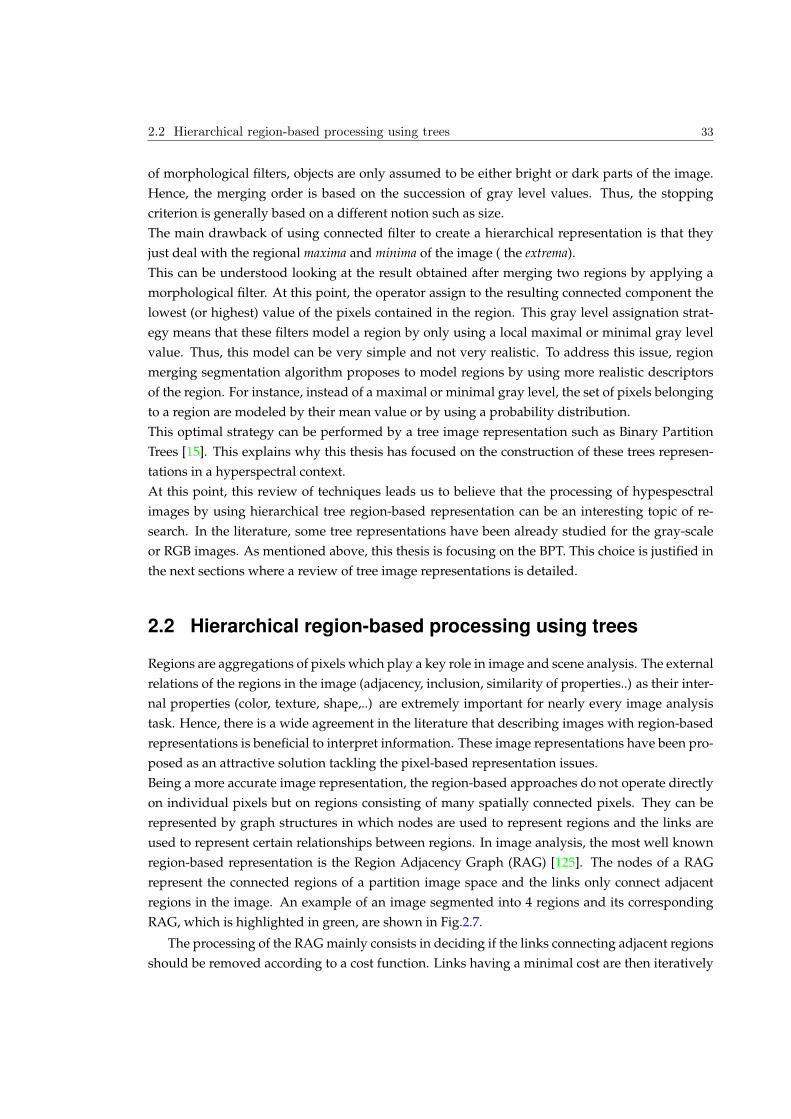
2.2 Hierarchical region-based processing using trees 33
of morphological filters, objects are only assumed to be either bright or dark parts of the image.
Hence, the merging order is based on the succession of gray level values. Thus, the stopping
criterion is generally based on a different notion such as size.
The main drawback of using connected filter to create a hierarchical representation is that they
just deal with the regional maxima and minima of the image ( the extrema).
This can be understood looking at the result obtained after merging two regions by applying a
morphological filter. At this point, the operator assign to the resulting connected component the
lowest (or highest) value of the pixels contained in the region. This gray level assignation strat-
egy means that these filters model a region by only using a local maximal or minimal gray level
value. Thus, this model can be very simple and not very realistic. To address this issue, region
merging segmentation algorithm proposes to model regions by using more realistic descriptors
of the region. For instance, instead of a maximal or minimal gray level, the set of pixels belonging
to a region are modeled by their mean value or by using a probability distribution.
This optimal strategy can be performed by a tree image representation such as Binary Partition
Trees [15]. This explains why this thesis has focused on the construction of these trees represen-
tations in a hyperspectral context.
At this point, this review of techniques leads us to believe that the processing of hypespesctral
images by using hierarchical tree region-based representation can be an interesting topic of re-
search. In the literature, some tree representations have been already studied for the gray-scale
or RGB images. As mentioned above, this thesis is focusing on the BPT. This choice is justified in
the next sections where a review of tree image representations is detailed.
2.2 Hierarchical region-based processing using trees
Regions are aggregations of pixels which play a key role in image and scene analysis. The external
relations of the regions in the image (adjacency, inclusion, similarity of properties..) as their inter-
nal properties (color, texture, shape,..) are extremely important for nearly every image analysis
task. Hence, there is a wide agreement in the literature that describing images with region-based
representations is beneficial to interpret information. These image representations have been pro-
posed as an attractive solution tackling the pixel-based representation issues.
Being a more accurate image representation, the region-based approaches do not operate directly
on individual pixels but on regions consisting of many spatially connected pixels. They can be
represented by graph structures in which nodes are used to represent regions and the links are
used to represent certain relationships between regions. In image analysis, the most well known
region-based representation is the Region Adjacency Graph (RAG) [125]. The nodes of a RAG
represent the connected regions of a partition image space and the links only connect adjacent
regions in the image. An example of an image segmented into 4 regions and its corresponding
RAG, which is highlighted in green, are shown in Fig.2.7.
The processing of the RAG mainly consists in deciding if the links connecting adjacent regions
should be removed according to a cost function. Links having a minimal cost are then iteratively
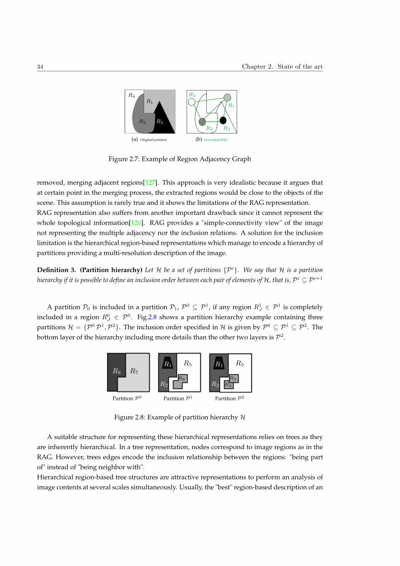
34 Chapter 2. State of the art
(a) Original partition (b) Associated RAG
R2
R2
R3
R3
R1
R1
R4R4
Figure 2.7: Example of Region Adjacency Graph
removed, merging adjacent regions[127]. This approach is very idealistic because it argues that
at certain point in the merging process, the extracted regions would be close to the objects of the
scene. This assumption is rarely true and it shows the limitations of the RAG representation.
RAG representation also suffers from another important drawback since it cannot represent the
whole topological information[126]. RAG provides a "simple-connectivity view" of the image
not representing the multiple adjacency nor the inclusion relations. A solution for the inclusion
limitation is the hierarchical region-based representations which manage to encode a hierarchy of
partitions providing a multi-resolution description of the image.
Definition 3. (Partition hierarchy) Let H be a set of partitions Pi. We say that H is a partition
hierarchy if it is possible to define an inclusion order between each pair of elements of H, that is, Pi Pi+1
A partition P0 is included in a partition P1, P0 P1, if any region R1J 2 P1 is completely
included in a region R0J 2 P0. Fig.2.8 shows a partition hierarchy example containing three
partitions H = P0 P1,P2. The inclusion order specified in H is given by P0 P1 P2. The
bottom layer of the hierarchy including more details than the other two layers is P2.
R1
R2
R1
R2
R3
R4
R6
R5 R5
R7R8
Partition P0 Partition P1 Partition P2
Figure 2.8: Example of partition hierarchy H
A suitable structure for representing these hierarchical representations relies on trees as they
are inherently hierarchical. In a tree representation, nodes correspond to image regions as in the
RAG. However, trees edges encode the inclusion relationship between the regions: "being part
of" instead of "being neighbor with".
Hierarchical region-based tree structures are attractive representations to perform an analysis of
image contents at several scales simultaneously. Usually, the "best" region-based description of an
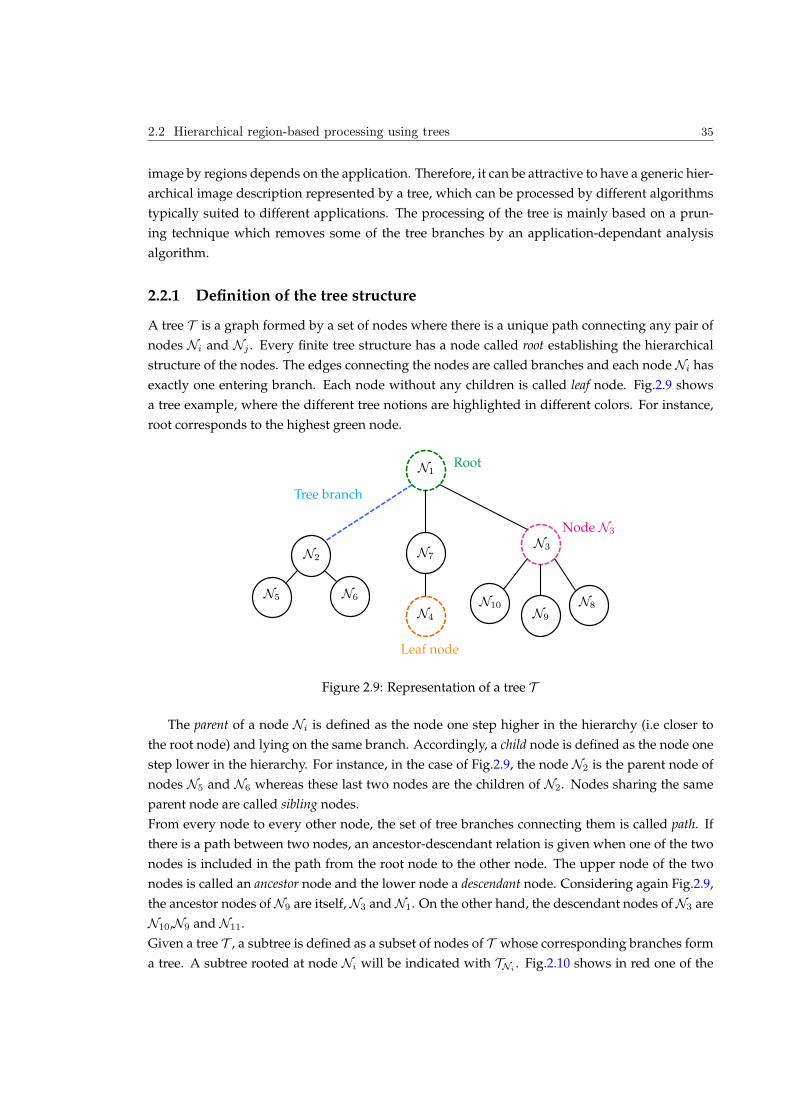
2.2 Hierarchical region-based processing using trees 35
image by regions depends on the application. Therefore, it can be attractive to have a generic hier-
archical image description represented by a tree, which can be processed by different algorithms
typically suited to different applications. The processing of the tree is mainly based on a prun-
ing technique which removes some of the tree branches by an application-dependant analysis
algorithm.
2.2.1 Definition of the tree structure
A tree T is a graph formed by a set of nodes where there is a unique path connecting any pair of
nodes Ni and Nj . Every finite tree structure has a node called root establishing the hierarchical
structure of the nodes. The edges connecting the nodes are called branches and each node Ni has
exactly one entering branch. Each node without any children is called leaf node. Fig.2.9 shows
a tree example, where the different tree notions are highlighted in different colors. For instance,
root corresponds to the highest green node.
N2
N4
N7N3
N8N9
N10N5 N6
N1
Tree branch
Root
Node N3
Leaf node
Figure 2.9: Representation of a tree T
The parent of a node Ni is defined as the node one step higher in the hierarchy (i.e closer to
the root node) and lying on the same branch. Accordingly, a child node is defined as the node one
step lower in the hierarchy. For instance, in the case of Fig.2.9, the node N2 is the parent node of
nodes N5 and N6 whereas these last two nodes are the children of N2. Nodes sharing the same
parent node are called sibling nodes.
From every node to every other node, the set of tree branches connecting them is called path. If
there is a path between two nodes, an ancestor-descendant relation is given when one of the two
nodes is included in the path from the root node to the other node. The upper node of the two
nodes is called an ancestor node and the lower node a descendant node. Considering again Fig.2.9,
the ancestor nodes of N9 are itself, N3 and N1. On the other hand, the descendant nodes of N3 are
N10,N9 and N11.
Given a tree T , a subtree is defined as a subset of nodes of T whose corresponding branches form
a tree. A subtree rooted at node Ni will be indicated with TNi. Fig.2.10 shows in red one of the
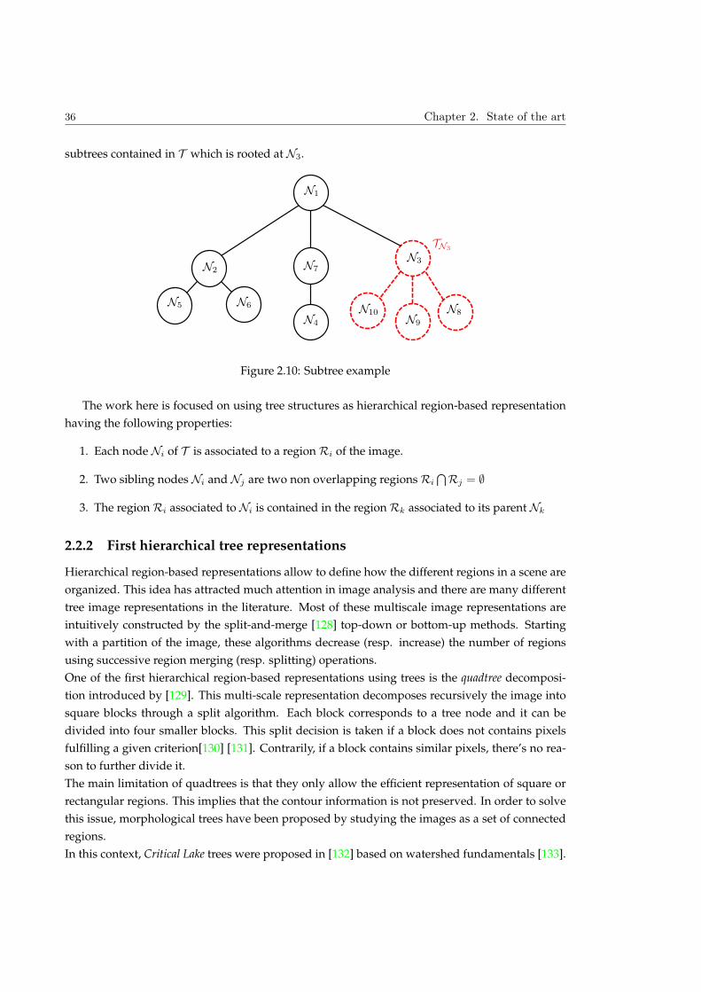
36 Chapter 2. State of the art
subtrees contained in T which is rooted at N3.
N2
N4
N7N3
N8N9
N10N5 N6
N1
TN3
Figure 2.10: Subtree example
The work here is focused on using tree structures as hierarchical region-based representation
having the following properties:
1. Each node Ni of T is associated to a region Ri of the image.
2. Two sibling nodes Ni and Nj are two non overlapping regions Ri
TRj = ;
3. The region Ri associated to Ni is contained in the region Rk associated to its parent Nk
2.2.2 First hierarchical tree representations
Hierarchical region-based representations allow to define how the different regions in a scene are
organized. This idea has attracted much attention in image analysis and there are many different
tree image representations in the literature. Most of these multiscale image representations are
intuitively constructed by the split-and-merge [128] top-down or bottom-up methods. Starting
with a partition of the image, these algorithms decrease (resp. increase) the number of regions
using successive region merging (resp. splitting) operations.
One of the first hierarchical region-based representations using trees is the quadtree decomposi-
tion introduced by [129]. This multi-scale representation decomposes recursively the image into
square blocks through a split algorithm. Each block corresponds to a tree node and it can be
divided into four smaller blocks. This split decision is taken if a block does not contains pixels
fulfilling a given criterion[130] [131]. Contrarily, if a block contains similar pixels, there’s no rea-
son to further divide it.
The main limitation of quadtrees is that they only allow the efficient representation of square or
rectangular regions. This implies that the contour information is not preserved. In order to solve
this issue, morphological trees have been proposed by studying the images as a set of connected
regions.
In this context, Critical Lake trees were proposed in [132] based on watershed fundamentals [133].
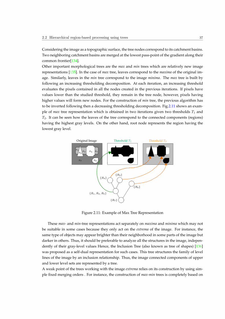
2.2 Hierarchical region-based processing using trees 37
Considering the image as a topographic surface, the tree nodes correspond to its catchment basins.
Two neighboring catchment basins are merged at the lowest pass-point of the gradient along their
common frontier[134].
Other important morphological trees are the max and min trees which are relatively new image
representations [135]. In the case of max tree, leaves correspond to the maxima of the original im-
age. Similarly, leaves in the min tree correspond to the image minima. The max tree is built by
following an increasing thresholding decomposition. At each iteration, an increasing threshold
evaluates the pixels contained in all the nodes created in the previous iterations. If pixels have
values lower than the studied threshold, they remain in the tree node, however, pixels having
higher values will form new nodes. For the construction of min tree, the previous algorithm has
to be inverted following then a decreasing thresholding decomposition. Fig.2.11 shows an exam-
ple of max tree representation which is obtained in two iterations given two thresholds T1 and
T2. It can be seen how the leaves of the tree correspond to the connected components (regions)
having the highest gray levels. On the other hand, root node represents the region having the
lowest gray level.
R7
R2
R6
R4
R1, R3, R5
Original Image Threshold T2Threshold T1
R2R3 R4 R5
R6R7
R1
Figure 2.11: Example of Max Tree Representation
These max- and min-tree representations act separately on maxima and minima which may not
be suitable in some cases because they only act on the extrema of the image. For instance, the
same type of objects may appear brighter than their neighborhood in some parts of the image but
darker in others. Thus, it should be preferable to analyze all the structures in the image, indepen-
dently of their gray-level values Hence, the Inclusion Tree (also known as tree of shapes) [136]
was proposed as a self-dual representation for such cases. This tree structures the family of level
lines of the image by an inclusion relationship. Thus, the image connected components of upper
and lower level sets are represented by a tree.
A weak point of the trees working with the image extrema relies on its construction by using sim-
ple fixed merging orders . For instance, the construction of max-min trees is completely based on
38 Chapter 2. State of the art
the absolute gray levels. Thus, they cannot describe easily objects that are not extrema. Therefore,
objects appearing in transition areas between extrema can be lost in the representation.
To address such limitation, the Binary Partition Tree was proposed as a more accurate image tree
representation being constructed by no fixed algorithm. This tree is a structured representation
of a set of hierarchical partitions which is usually obtained through a segmentation algorithm.
2.2.3 BPT Literature
The Binary Partition Tree [15] is a hierarchy of regions representing the image at different reso-
lution levels. The BPT allows the assignment of spatial constraints and the definition of partial
orders of the regions. The hierarchy of partitions contained in BPT gives a much more natural
representation of visual scenes. This addresses the weaknesses of working with the perceptually
meaningless entities offered by the pixel-based representation (the pixel grid).
In the literature, BPTs have been previously studied showing their effectiveness in image filtering
[15], object extraction [39] [43] [45], segmentation [44] [24], motion compensation [38], filtering
[138] or contour detection [46]. Hence, the construction of BPTs has been an area of research in
the last ten years in the context of multimedia images and RGB images. This construction is based
on the definition of an iterative region-merging algorithm.
In image processing, the construction of a region merging order has to deal with the two follow-
ing questions: 1) how to model a region and 2) how to decide if two regions are similar or not.
For the first aspect, most of the region merging algorithms proposed by BPT construction have
used as region model the mean color value of the pixels belonging to the region [15] [40]. This
model used also in [41] corresponds to a zero-order model which assumes color homogeneity in-
side the region. Because this assumption is rarely true, a model for the images formed by textured
regions has been proposed in [42]. Note that this last approach assumes either color homogeneous
or textured regions. In order to propose a more general strategy, a non parametric statistical region
model has been proposed in [17]. This model corresponds to set of non parametric probability
density functions (pdfs) with no assumptions about the nature of the regions nor the shape of the
pdfs. Other important approaches have been proposed to use region models including shape in-
formation. In [47], syntactic properties directly related to the region shape description have been
introduced. The use of syntactic visual features in region merging algorithm has also been used
in [48] dividing the merging process into stages and using a different homogeneity criterion at
each stage. Also, in [39] the perimeter of the regions is considered as a region model descriptor.
The second important aspect for constructing the merging order is how to measure the similar-
ity between regions. The answer to this question is given by the merging criterion definition.
The merging criterion corresponds to a similarity measure between the regions, which are previ-
ously modeled by the chosen region model. Thus, the merging criterion used in a region merging
algorithm is completely linked to the region model definition. Using a zero-order model, merg-
ing criteria are mainly defined by classical distance based on absolute difference between colors.
A complete study can be found in [40], where different measures using the classical Euclidean
distance are compared. In the case of non-parametric statistical models, their use requires the
2.3 Conclusions 39
definition of a robust distance between probability distributions. In [17], some statistical similar-
ity measures such as the Kullback-Leibler divergence rate, the Bhattacharyya coefficient and the
first order Markov empirical transition matrices are proposed.
As mentioned before, the construction of BPT offers a generic representation of the image. This
is very important and it is the main reason why BPT has been used in various applications. Each
application is associated to a tree processing technique corresponding to the tree pruning[137].
Previous works have presented different tree pruning techniques for different purposes. A first
category of the proposed pruning techniques are based on increasing criteria along the branches.
A criterion C assessed on a region is increasing if: 8R1 R2 =) C(R1) C(R2). This implies
that if a criterion C(Ni) is associated to a node Ni, the criterion value for the parent node of Ni will
be higher. As a result, if a node should be removed by the pruning technique, all its descendant
should also be removed. Thus, the pruning technique is straightforward by removing the subtree
rooted by a node for which the criterion is below a given threshold. An example can be found
in [49] where a BPT pruning by region evolution [56] is presented in an object extraction context.
Increasing criteria have been frequently used because they directly lead to a pruning strategy.
Non-increasing criteria have been also proposed as the basis of the pruning strategy for some
applications. These strategies are more difficult because the descendants of a node to be removed
have not necessarily to be removed.
Formulating the problem as a dynamic programming issue, a pruning algorithm based on the
Viterbi algorithm was presented for filtering purposes in [15] [135]. In the context of object de-
tection, some pruning techniques are formulated as node detection[39] [43]. Defining a set of
descriptors of the sought objects, these algorithms look for the nodes most likely corresponding
to the sought object. More recently, a pruning technique has been proposed in [138] for filtering
speckle noise. Studying a homogeneity measure along branches, this pruning follows a max rule
which prunes the branches from the leaves up to the first node that has to be preserved.
Another family of pruning relies on a global minimization of a criterion under constraint. This
problem is then formulated as a global energy minimization problem by using a Lagrangian func-
tion. In this approach, the lagrangian parameter λ is balancing the criterion and a smoothing
related to the constraint. Using a gradient descent method, the optimal λ value is computed and
the partition associated to the λ parameter defines the global pruning.
Setting a rate/distortion criterion, a pruning strategy following this approach has been proposed
in [139]. Following this idea, a pruning algorithm by using a dynamic programming principle
has been defined to compute the optimal pruning with respect to any value of λ [140].
2.3 Conclusions
In this chapter we have reviewed the work done so far in the areas of hyperspectral image pro-
cessing and of hierarchical region-based tree representations. Most of the relevant work in hy-
perspectral imaging has been explained detailing how the main drawbacks of HSI processing are
addressed. Some of these issues have been presented as the incorporation of the spatial informa-
40 Chapter 2. State of the art
tion to process or classify the data, the dimensionality reduction of the image before processing
the extension of classical techniques to HSI context or the definition of a vector order to define
morphological tools.
A large number of techniques have shown in Sec.2.1.1 how the incorporation of the spatial in-
formation can be introduced as a methodology stage from different manners. All the reviewed
techniques working in the spatial-spectral domain process hyperspectral data by using their pixel-
based representation.
As mentioned before, this low level representation provides extremely local information since the
decisions and processing steps are applied individually to all pixels. Consequently, this low scale
representation is in most cases too far from the semantic interpretation scale. To manage this is-
sue, some of these techniques such as ECHO, have tried to introduce a description of the image,
as region-based partition, as an input parameter in their strategy.
This gap between image representation and semantic interpretation has been also addressed by
hierarchical segmentations described in Sec.2.1.2. In a hyperspectral framework, these techniques
have been suggested to provide a region-based description of the image at different scales. Unfor-
tunately, hierarchical segmentations cannot be considered as a generic region-based image repre-
sentation which can be used to address a large number of applications.
A solution for constructing a generic representation, structuring the different regions in an orga-
nized way, relies on trees. This idea has been reviewed in Sec.2.2. This section has introduced
the main advantages of processing images using tree structures. Some classical tree-based im-
ages representations previously introduced for gray-scale or RGB images have been reviewed.
Morphological trees have been explained in Sec.2.2.2. They offer them a solution for the contour
preservation problem related to Quad-Trees. Concerning morphological trees, some limitations
have also been explained. To address such problems, BPTs have been presented as a powerful
image representation that can be constructed using them by performing a region merging algo-
rithm.
The BPT literature for classical imagery has been presented in Sec.2.2.3 where the different merg-
ing orders proposed for BPT construction have been mentioned. Also in this section, BPT pruning
strategies have been reviewed showing the advantages of tree processing.
As a conclusion, this chapter has presented the framework of this thesis describing the necessity
of the construction of a hierarchical region-based representation as Binary Partition Tree. The fol-
lowing chapters will address the construction of BPT representation for hyperspectral images and
their processing for various specific applications.

3BPT construction
Contents
3.1 Introduction . . . . . . . . . . . . . . . . . . . . . . . . . . . . . . . . . . . . . . . . 42
3.2 Region Model . . . . . . . . . . . . . . . . . . . . . . . . . . . . . . . . . . . . . . . 45
3.2.1 First-order parametric model . . . . . . . . . . . . . . . . . . . . . . . . . . . 46
3.2.2 Non parametric statistical Region Model . . . . . . . . . . . . . . . . . . . . 47
3.3 Merging Criterion . . . . . . . . . . . . . . . . . . . . . . . . . . . . . . . . . . . . . 55
3.3.1 Measures associated to the first-order parametric model . . . . . . . . . . . 59
3.3.2 Measures associated to the non parametrical statistical region model . . . . 61
3.3.3 Similarity measure via Multidimensional Scaling . . . . . . . . . . . . . . . 64
3.4 Experimental Evaluation . . . . . . . . . . . . . . . . . . . . . . . . . . . . . . . . . 71
3.4.1 Quality measures between partitions . . . . . . . . . . . . . . . . . . . . . . 71
3.4.2 Data Sets Definition . . . . . . . . . . . . . . . . . . . . . . . . . . . . . . . . 73
3.4.3 Experiment 1: Evaluation of BPT hierarchical levels . . . . . . . . . . . . . . 78
3.4.4 Experiment 2: Evaluation of Ds selection . . . . . . . . . . . . . . . . . . . . 93
3.5 Conclusions . . . . . . . . . . . . . . . . . . . . . . . . . . . . . . . . . . . . . . . . 94
This chapter details the construction of BPT representation for hyperspectral imaging. In this
framework, different region merging algorithms are discussed by studying various region mod-
els and merging criteria. The hierarchical partitions obtained during the BPT construction are
evaluated and compared with other state-of-the-art region merging techniques[22].
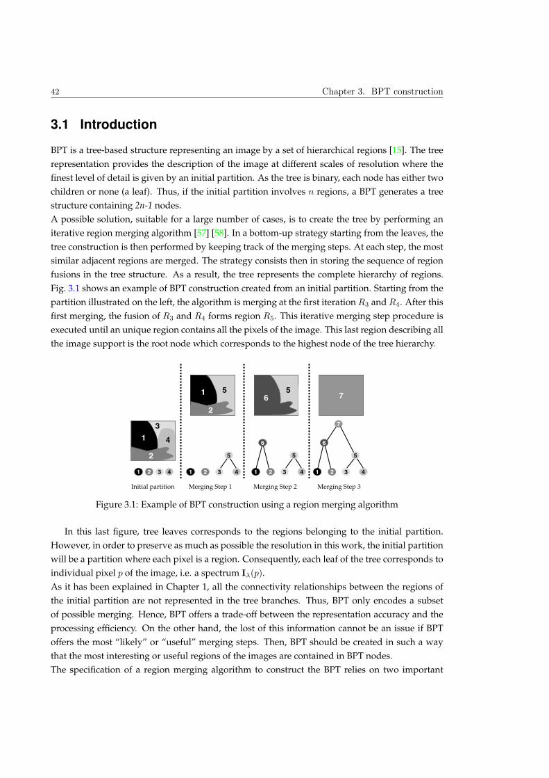
42 Chapter 3. BPT construction
3.1 Introduction
BPT is a tree-based structure representing an image by a set of hierarchical regions [15]. The tree
representation provides the description of the image at different scales of resolution where the
finest level of detail is given by an initial partition. As the tree is binary, each node has either two
children or none (a leaf). Thus, if the initial partition involves n regions, a BPT generates a tree
structure containing 2n-1 nodes.
A possible solution, suitable for a large number of cases, is to create the tree by performing an
iterative region merging algorithm [57] [58]. In a bottom-up strategy starting from the leaves, the
tree construction is then performed by keeping track of the merging steps. At each step, the most
similar adjacent regions are merged. The strategy consists then in storing the sequence of region
fusions in the tree structure. As a result, the tree represents the complete hierarchy of regions.
Fig. 3.1 shows an example of BPT construction created from an initial partition. Starting from the
partition illustrated on the left, the algorithm is merging at the first iteration R3 and R4. After this
first merging, the fusion of R3 and R4 forms region R5. This iterative merging step procedure is
executed until an unique region contains all the pixels of the image. This last region describing all
the image support is the root node which corresponds to the highest node of the tree hierarchy.
1
2
3
4
1
2
56
5
3 4
5
1 23 41 2 3 4
5
1 2
6
7
3 4
5
1 2
6
7
Original PartitionInitial partition Merging Step 1 Merging Step 2 Merging Step 3
Figure 3.1: Example of BPT construction using a region merging algorithm
In this last figure, tree leaves corresponds to the regions belonging to the initial partition.
However, in order to preserve as much as possible the resolution in this work, the initial partition
will be a partition where each pixel is a region. Consequently, each leaf of the tree corresponds to
individual pixel p of the image, i.e. a spectrum Iλ(p).
As it has been explained in Chapter 1, all the connectivity relationships between the regions of
the initial partition are not represented in the tree branches. Thus, BPT only encodes a subset
of possible merging. Hence, BPT offers a trade-off between the representation accuracy and the
processing efficiency. On the other hand, the lost of this information cannot be an issue if BPT
offers the most “likely” or “useful” merging steps. Then, BPT should be created in such a way
that the most interesting or useful regions of the images are contained in BPT nodes.
The specification of a region merging algorithm to construct the BPT relies on two important
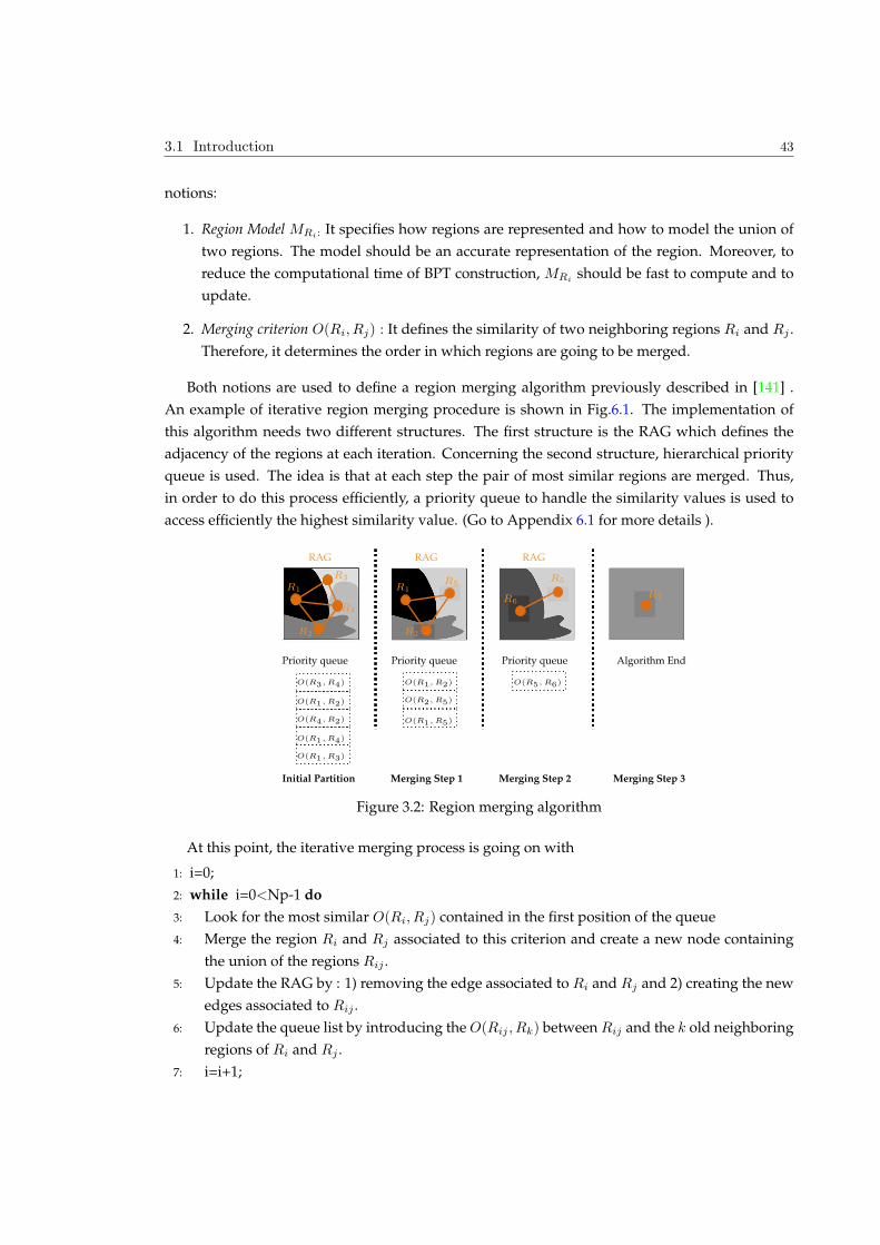
3.1 Introduction 43
notions:
1. Region Model MRi: It specifies how regions are represented and how to model the union of
two regions. The model should be an accurate representation of the region. Moreover, to
reduce the computational time of BPT construction, MRishould be fast to compute and to
update.
2. Merging criterion O(Ri, Rj) : It defines the similarity of two neighboring regions Ri and Rj .
Therefore, it determines the order in which regions are going to be merged.
Both notions are used to define a region merging algorithm previously described in [141] .
An example of iterative region merging procedure is shown in Fig.6.1. The implementation of
this algorithm needs two different structures. The first structure is the RAG which defines the
adjacency of the regions at each iteration. Concerning the second structure, hierarchical priority
queue is used. The idea is that at each step the pair of most similar regions are merged. Thus,
in order to do this process efficiently, a priority queue to handle the similarity values is used to
access efficiently the highest similarity value. (Go to Appendix 6.1 for more details ).
Priority queue
O(R3, R4) O(R1, R2)
O(R2, R5)
O(R1, R5)
O(R5, R6)
O(R1, R2)
O(R4, R2)
O(R1, R4)
O(R1, R3)
RAG
R1
R3
R4
R2
Priority queue
RAG
R1
R2
R5
Priority queue
RAG
R6
R5
Algorithm End
R7
Initial Partition Merging Step 1 Merging Step 2 Merging Step 3
Figure 3.2: Region merging algorithm
At this point, the iterative merging process is going on with
1: i=0;
2: while i=0<Np-1 do
3: Look for the most similar O(Ri, Rj) contained in the first position of the queue
4: Merge the region Ri and Rj associated to this criterion and create a new node containing
the union of the regions Rij .
5: Update the RAG by : 1) removing the edge associated to Ri and Rj and 2) creating the new
edges associated to Rij .
6: Update the queue list by introducing the O(Rij , Rk) between Rij and the k old neighboring
regions of Ri and Rj .
7: i=i+1;
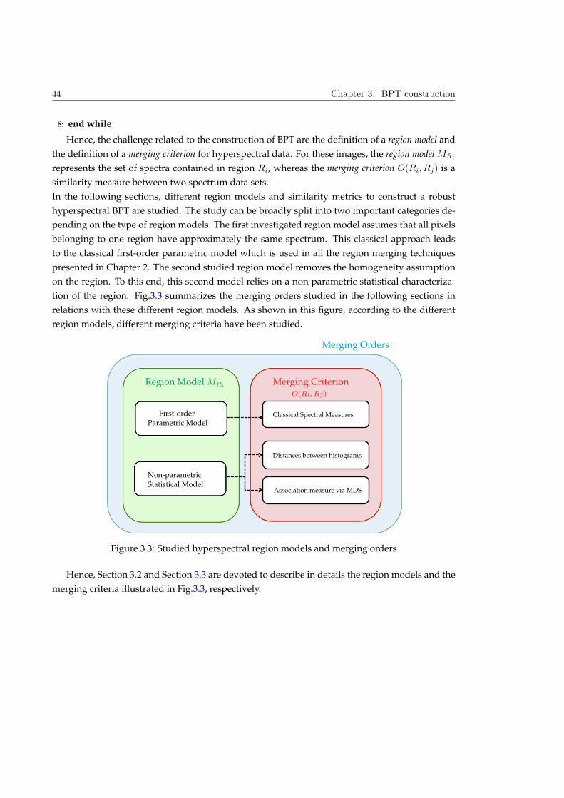
44 Chapter 3. BPT construction
8: end while
Hence, the challenge related to the construction of BPT are the definition of a region model and
the definition of a merging criterion for hyperspectral data. For these images, the region model MRi
represents the set of spectra contained in region Ri, whereas the merging criterion O(Ri, Rj) is a
similarity measure between two spectrum data sets.
In the following sections, different region models and similarity metrics to construct a robust
hyperspectral BPT are studied. The study can be broadly split into two important categories de-
pending on the type of region models. The first investigated region model assumes that all pixels
belonging to one region have approximately the same spectrum. This classical approach leads
to the classical first-order parametric model which is used in all the region merging techniques
presented in Chapter 2. The second studied region model removes the homogeneity assumption
on the region. To this end, this second model relies on a non parametric statistical characteriza-
tion of the region. Fig.3.3 summarizes the merging orders studied in the following sections in
relations with these different region models. As shown in this figure, according to the different
region models, different merging criteria have been studied.
Region Model MRiMerging Criterion
O(Ri,Rj)
Classical Spectral Measures
Distances between histograms
Association measure via MDS
First-orderParametric Model
Non-parametricStatistical Model
Merging Orders
Figure 3.3: Studied hyperspectral region models and merging orders
Hence, Section 3.2 and Section 3.3 are devoted to describe in details the region models and the
merging criteria illustrated in Fig.3.3, respectively.
3.2 Region Model 45
3.2 Region Model
In hyperspectral image analysis, an image region R is defined as a set of connected NRppixels,
corresonding to spectra. In this spectrum data set R = Iλ(p1), Iλ(p2), .....Iλ(pNRp), each pixel is
described by pj and a spectrum Iλ(pj) formed by Nz radiance values. The model of a region MR
is an approximate description of the NR spectra describing the relevant information about region
R.
Region modeling for hyperspectral data is challenging because the goal is to make full use of the
greater discrimination provided by the high spectral resolution. The main issue is the variations
of the spectral reflectance curve, within the spectra forming a region of the same class material.
The spatial and spectral patterns are characteristic of the material itself, and they introduce a de-
gree of uncertainty arising from inhomogeneities and natural variations within the material. For
example, if the goal is to model a large vegetation region formed by healthy and stressed grass. In
this case, all the spectra forming the region may be in fact almost identical, however, this region
will not have an unimodal behavior.
Past hyperspectral works focusing on spectral classification and hierarchical segmentation have
presented different strategies to model a set of spectra [19] [22][9]. Although these classification
and segmentation algorithms have tried to model spectral data sets, there is an important dif-
ference between them. In hierarchical segmentation methods, each modeled spectrum data set
forms a region, i.e. the spectra are connected in the spatial domain. Contrarily, in the case of
spectral classification techniques, spectrum data sets are sets of unconnected spectra. Therefore,
in this last case, spectrum data sets are only groups of spectra having "similar behaviors" in the
spectral domain.
In the case of hierarchical segmentations [82] [117] [22], the most popular solution to describe a
set of spectra is the first-order parametric model, that is the mean spectrum. As detailed in the
following, the key of this model’s popularity is its simplicity which allows to define merging or-
ders in a simple way. However, this model can have an important drawback because it assumes
spatial homogeneity inside the region. In order to solve this problem, parametric models for hy-
perspectral data have also been studied for some approaches [81]. In this case, the strategy is to
model regions by a gaussian probability density function by estimating its mean and covariance
matrix. This model presents two important drawbacks: 1) the estimation of the covariance matrix
is not easy, in particular for small regions and 2) this model, as in the case of first order model, is
also unimodal.
The unimodality problem has been addressed in several classification (also clustering) techniques.
The most well-known solution consists in modeling a spectrum data set assuming that spectra
belonging to the same group (cluster) are drawn from a multivariate Gaussian probability dis-
tribution. Thus, a group of spectra can be statistically modeled by a parametric probability den-
sity function completely specified by parameters as multivariate means and covariance matrices.
Note that these models are obtained through a training phase, therefore, the performances of this
modeling approach largely rely on the number of training samples for each class. This implies
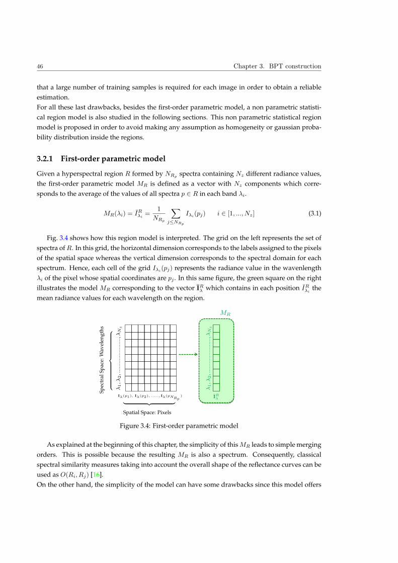
46 Chapter 3. BPT construction
that a large number of training samples is required for each image in order to obtain a reliable
estimation.
For all these last drawbacks, besides the first-order parametric model, a non parametric statisti-
cal region model is also studied in the following sections. This non parametric statistical region
model is proposed in order to avoid making any assumption as homogeneity or gaussian proba-
bility distribution inside the regions.
3.2.1 First-order parametric model
Given a hyperspectral region R formed by NRpspectra containing Nz different radiance values,
the first-order parametric model MR is defined as a vector with Nz components which corre-
sponds to the average of the values of all spectra p 2 R in each band λi.
MR(λi) = IRλi=
1
NRp
X
jNRp
Iλi(pj) i 2 [1, ..., Nz] (3.1)
Fig. 3.4 shows how this region model is interpreted. The grid on the left represents the set of
spectra of R. In this grid, the horizontal dimension corresponds to the labels assigned to the pixels
of the spatial space whereas the vertical dimension corresponds to the spectral domain for each
spectrum. Hence, each cell of the grid Iλi(pj) represents the radiance value in the wavenlength
λi of the pixel whose spatial coordinates are pj . In this same figure, the green square on the right
illustrates the model MR corresponding to the vector IRλ which contains in each position IRλithe
mean radiance values for each wavelength on the region.
MR
λ1,λ2,......................,λN
z
λ1,λ2,......................,λN
z
Iλ(p1), Iλ(p2), ....., Iλ(pNRp) I
Rλ
z|
| z
Spatial Space: Pixels
Sp
ectr
alS
pac
e:W
avel
eng
ths
Figure 3.4: First-order parametric model
As explained at the beginning of this chapter, the simplicity of this MR leads to simple merging
orders. This is possible because the resulting MR is also a spectrum. Consequently, classical
spectral similarity measures taking into account the overall shape of the reflectance curves can be
used as O(Ri, Rj) [16].
On the other hand, the simplicity of the model can have some drawbacks since this model offers
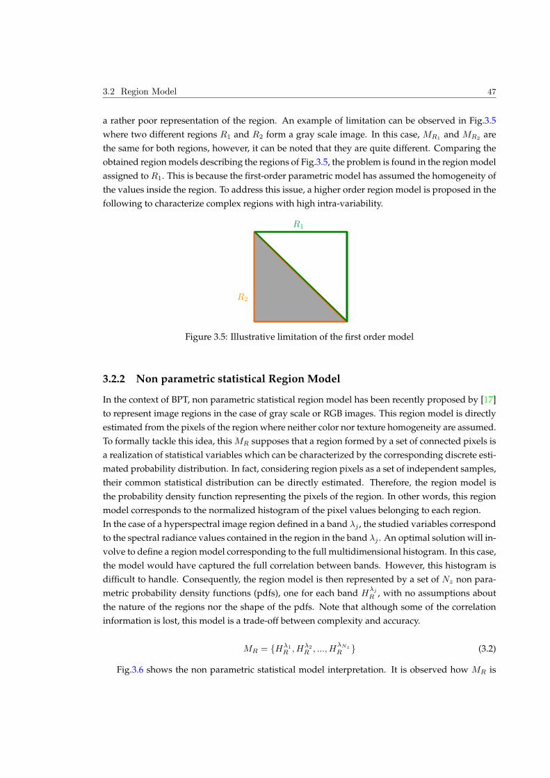
3.2 Region Model 47
a rather poor representation of the region. An example of limitation can be observed in Fig.3.5
where two different regions R1 and R2 form a gray scale image. In this case, MR1and MR2
are
the same for both regions, however, it can be noted that they are quite different. Comparing the
obtained region models describing the regions of Fig.3.5, the problem is found in the region model
assigned to R1. This is because the first-order parametric model has assumed the homogeneity of
the values inside the region. To address this issue, a higher order region model is proposed in the
following to characterize complex regions with high intra-variability.
R1
R2
Figure 3.5: Illustrative limitation of the first order model
3.2.2 Non parametric statistical Region Model
In the context of BPT, non parametric statistical region model has been recently proposed by [17]
to represent image regions in the case of gray scale or RGB images. This region model is directly
estimated from the pixels of the region where neither color nor texture homogeneity are assumed.
To formally tackle this idea, this MR supposes that a region formed by a set of connected pixels is
a realization of statistical variables which can be characterized by the corresponding discrete esti-
mated probability distribution. In fact, considering region pixels as a set of independent samples,
their common statistical distribution can be directly estimated. Therefore, the region model is
the probability density function representing the pixels of the region. In other words, this region
model corresponds to the normalized histogram of the pixel values belonging to each region.
In the case of a hyperspectral image region defined in a band λj , the studied variables correspond
to the spectral radiance values contained in the region in the band λj . An optimal solution will in-
volve to define a region model corresponding to the full multidimensional histogram. In this case,
the model would have captured the full correlation between bands. However, this histogram is
difficult to handle. Consequently, the region model is then represented by a set of Nz non para-
metric probability density functions (pdfs), one for each band Hλj
R , with no assumptions about
the nature of the regions nor the shape of the pdfs. Note that although some of the correlation
information is lost, this model is a trade-off between complexity and accuracy.
MR = Hλ1
R , Hλ2
R , ..., HλNz
R (3.2)
Fig.3.6 shows the non parametric statistical model interpretation. It is observed how MR is
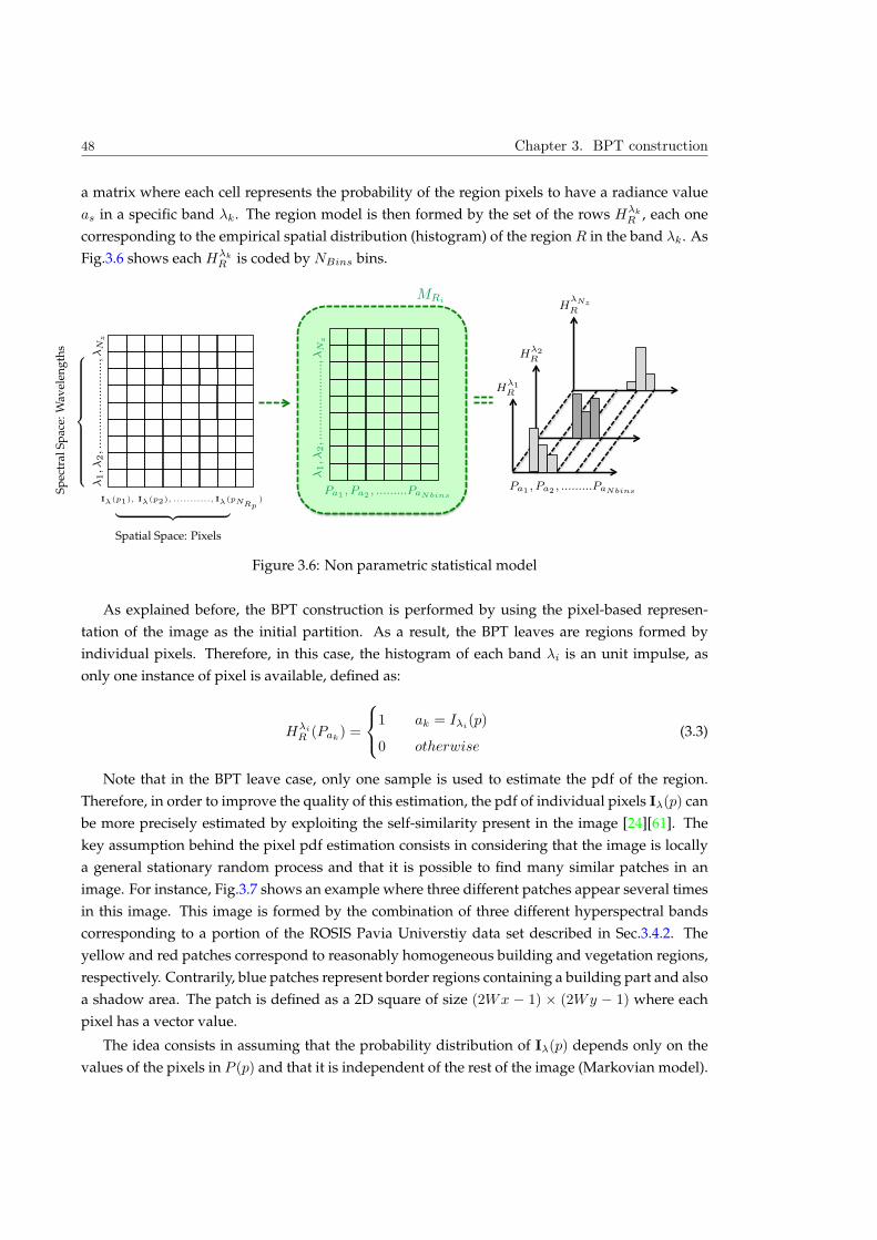
48 Chapter 3. BPT construction
a matrix where each cell represents the probability of the region pixels to have a radiance value
as in a specific band λk. The region model is then formed by the set of the rows Hλk
R , each one
corresponding to the empirical spatial distribution (histogram) of the region R in the band λk. As
Fig.3.6 shows each Hλk
R is coded by NBins bins.
MRi
λ1,λ2,......................,λN
z
λ1,λ2,.........................,λN
z
Iλ(p1), Iλ(p2), ..........., Iλ(pNRp)
Pa1 , Pa2 , .........PaNbinsPa1 , Pa2 , .........PaNbins
Hλ2R
HλNzR
Hλ1R
z|
| z
Spatial Space: Pixels
Sp
ectr
alS
pac
e:W
avel
eng
ths
Figure 3.6: Non parametric statistical model
As explained before, the BPT construction is performed by using the pixel-based represen-
tation of the image as the initial partition. As a result, the BPT leaves are regions formed by
individual pixels. Therefore, in this case, the histogram of each band λi is an unit impulse, as
only one instance of pixel is available, defined as:
Hλi
R (Pak) =
8
<
:
1 ak = Iλi(p)
0 otherwise(3.3)
Note that in the BPT leave case, only one sample is used to estimate the pdf of the region.
Therefore, in order to improve the quality of this estimation, the pdf of individual pixels Iλ(p) can
be more precisely estimated by exploiting the self-similarity present in the image [24][61]. The
key assumption behind the pixel pdf estimation consists in considering that the image is locally
a general stationary random process and that it is possible to find many similar patches in an
image. For instance, Fig.3.7 shows an example where three different patches appear several times
in this image. This image is formed by the combination of three different hyperspectral bands
corresponding to a portion of the ROSIS Pavia Universtiy data set described in Sec.3.4.2. The
yellow and red patches correspond to reasonably homogeneous building and vegetation regions,
respectively. Contrarily, blue patches represent border regions containing a building part and also
a shadow area. The patch is defined as a 2D square of size (2Wx − 1) (2Wy − 1) where each
pixel has a vector value.
The idea consists in assuming that the probability distribution of Iλ(p) depends only on the
values of the pixels in P (p) and that it is independent of the rest of the image (Markovian model).
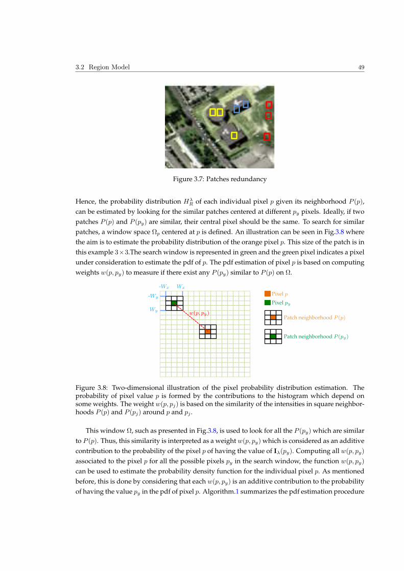
3.2 Region Model 49
Figure 3.7: Patches redundancy
Hence, the probability distribution HλR of each individual pixel p given its neighborhood P (p),
can be estimated by looking for the similar patches centered at different py pixels. Ideally, if two
patches P (p) and P (py) are similar, their central pixel should be the same. To search for similar
patches, a window space Ωp centered at p is defined. An illustration can be seen in Fig.3.8 where
the aim is to estimate the probability distribution of the orange pixel p. This size of the patch is in
this example 33.The search window is represented in green and the green pixel indicates a pixel
under consideration to estimate the pdf of p. The pdf estimation of pixel p is based on computing
weights w(p, py) to measure if there exist any P (py) similar to P (p) on Ω.
Wx-Wx
-Wy
Wy
Pixel p
Pixel py
w(p, py)Patch neighborhood P (p)
Patch neighborhood P (py)
Figure 3.8: Two-dimensional illustration of the pixel probability distribution estimation. Theprobability of pixel value p is formed by the contributions to the histogram which depend onsome weights. The weight w(p, pj) is based on the similarity of the intensities in square neighbor-hoods P (p) and P (pj) around p and pj .
This window Ω, such as presented in Fig.3.8, is used to look for all the P (py) which are similar
to P (p). Thus, this similarity is interpreted as a weight w(p, py) which is considered as an additive
contribution to the probability of the pixel p of having the value of Iλ(py). Computing all w(p, py)
associated to the pixel p for all the possible pixels py in the search window, the function w(p, py)
can be used to estimate the probability density function for the individual pixel p. As mentioned
before, this is done by considering that each w(p, py) is an additive contribution to the probability
of having the value py in the pdf of pixel p. Algorithm.1 summarizes the pdf estimation procedure
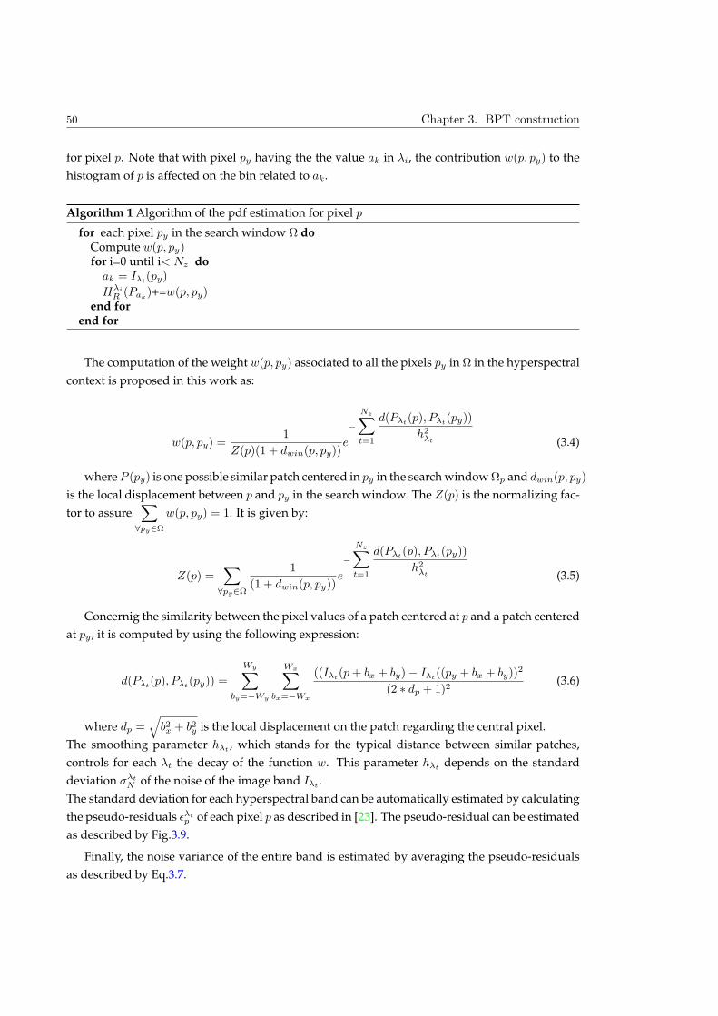
50 Chapter 3. BPT construction
for pixel p. Note that with pixel py having the the value ak in λi, the contribution w(p, py) to the
histogram of p is affected on the bin related to ak.
Algorithm 1 Algorithm of the pdf estimation for pixel p
for each pixel py in the search window Ω doCompute w(p, py)for i=0 until i< Nz doak = Iλi
(py)
Hλi
R (Pak)+=w(p, py)
end forend for
The computation of the weight w(p, py) associated to all the pixels py in Ω in the hyperspectral
context is proposed in this work as:
w(p, py) =1
Z(p)(1 + dwin(p, py))e
−
NzX
t=1
d(Pλt(p), Pλt
(py))
h2λt (3.4)
where P (py) is one possible similar patch centered in py in the search window Ωp and dwin(p, py)
is the local displacement between p and py in the search window. The Z(p) is the normalizing fac-
tor to assureX
8py2Ω
w(p, py) = 1. It is given by:
Z(p) =X
8py2Ω
1
(1 + dwin(p, py))e
−
NzX
t=1
d(Pλt(p), Pλt
(py))
h2λt (3.5)
Concernig the similarity between the pixel values of a patch centered at p and a patch centered
at py , it is computed by using the following expression:
d(Pλt(p), Pλt
(py)) =
WyX
by=−Wy
WxX
bx=−Wx
((Iλt(p+ bx + by)− Iλt
((py + bx + by))2
(2 dp + 1)2(3.6)
where dp =q
b2x + b2y is the local displacement on the patch regarding the central pixel.
The smoothing parameter hλt, which stands for the typical distance between similar patches,
controls for each λt the decay of the function w. This parameter hλtdepends on the standard
deviation σλt
N of the noise of the image band Iλt.
The standard deviation for each hyperspectral band can be automatically estimated by calculating
the pseudo-residuals λtp of each pixel p as described in [23]. The pseudo-residual can be estimated
as described by Fig.3.9.
Finally, the noise variance of the entire band is estimated by averaging the pseudo-residuals
as described by Eq.3.7.
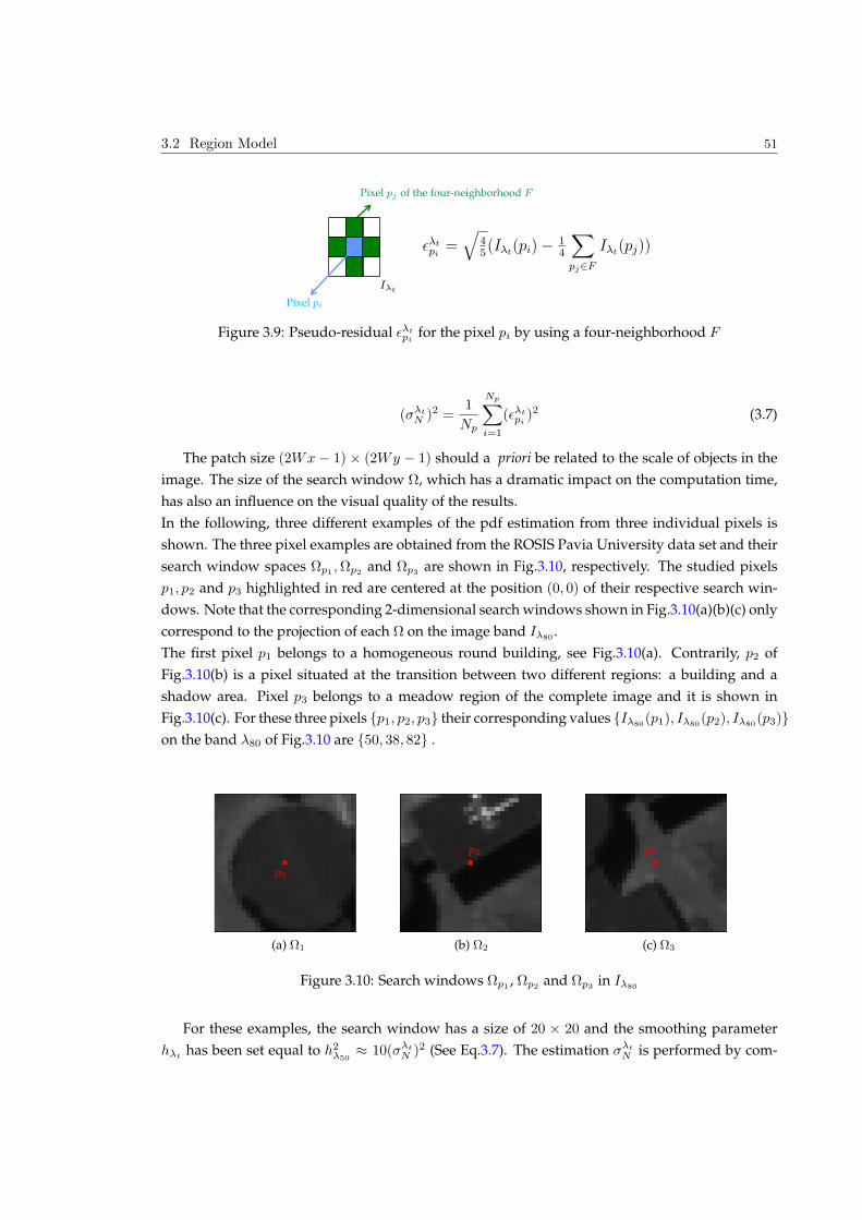
3.2 Region Model 51
Pixel pi
Pixel pj of the four-neighborhood F
ελtpi
=q
45(Iλt
(pi)−14
X
pj∈F
Iλt(pj))
Iλt
Figure 3.9: Pseudo-residual λtpi
for the pixel pi by using a four-neighborhood F
(σλt
N )2 =1
Np
NpX
i=1
(λtpi)2 (3.7)
The patch size (2Wx − 1) (2Wy − 1) should a priori be related to the scale of objects in the
image. The size of the search window Ω, which has a dramatic impact on the computation time,
has also an influence on the visual quality of the results.
In the following, three different examples of the pdf estimation from three individual pixels is
shown. The three pixel examples are obtained from the ROSIS Pavia University data set and their
search window spaces Ωp1,Ωp2
and Ωp3are shown in Fig.3.10, respectively. The studied pixels
p1, p2 and p3 highlighted in red are centered at the position (0, 0) of their respective search win-
dows. Note that the corresponding 2-dimensional search windows shown in Fig.3.10(a)(b)(c) only
correspond to the projection of each Ω on the image band Iλ80.
The first pixel p1 belongs to a homogeneous round building, see Fig.3.10(a). Contrarily, p2 of
Fig.3.10(b) is a pixel situated at the transition between two different regions: a building and a
shadow area. Pixel p3 belongs to a meadow region of the complete image and it is shown in
Fig.3.10(c). For these three pixels p1, p2, p3 their corresponding values Iλ80(p1), Iλ80(p2), Iλ80(p3)
on the band λ80 of Fig.3.10 are 50, 38, 82 .
(a) Ω1
p1
(b) Ω2
p2
(c) Ω3
p3
Figure 3.10: Search windows Ωp1 , Ωp2 and Ωp3 in Iλ80
For these examples, the search window has a size of 20 20 and the smoothing parameter
hλthas been set equal to h2
λ50 10(σλt
N )2 (See Eq.3.7). The estimation σλt
N is performed by com-
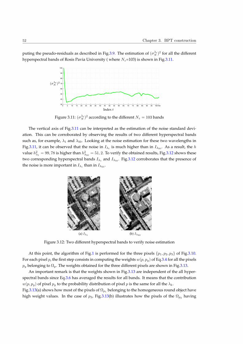
52 Chapter 3. BPT construction
puting the pseudo-residuals as described in Fig.3.9. The estimation of (σλt
N )2 for all the different
hyperspectral bands of Rosis Pavia University ( where Nz=103) is shown in Fig.3.11.
0 5 10 15 20 25 30 35 40 45 50 55 60 65 70 75 80 85 90 95 10010330
40
50
60
70
80
90
100
Index t
(σλtN
)2
Figure 3.11: (σλt
N )2 according to the different Nz = 103 bands
The vertical axis of Fig.3.11 can be interpreted as the estimation of the noise standard devi-
ation. This can be corroborated by observing the results of two different hyperspectral bands
such as, for example, λ1 and λ50. Looking at the noise estimation for these two wavelengths in
Fig.3.11, it can be observed that the noise in Iλ1is much higher than in Iλ50
. As a result, the h
value h2λ1
= 99, 78 is higher than h2λ50
= 51, 2. To verify the obtained results, Fig.3.12 shows these
two corresponding hyperspectral bands Iλ1and Iλ50
. Fig.3.12 corroborates that the presence of
the noise is more important in Iλ1than in Iλ50
.
(a) Iλ1(b) Iλ50
Figure 3.12: Two different hyperspectral bands to verify noise estimation
At this point, the algorithm of Fig.1 is performed for the three pixels p1, p2, p3 of Fig.3.10.
For each pixel p, the first step consists in computing the weights w(p, py) of Eq.3.4 for all the pixels
py belonging to Ωp. The weights obtained for the three different pixels are shown in Fig.3.13.
An important remark is that the weights shown in Fig.3.13 are independent of the all hyper-
spectral bands since Eq.3.6 has averaged the results for all bands. It means that the contribution
w(p, py) of pixel py to the probability distribution of pixel p is the same for all the λk.
Fig.3.13(a) shows how most of the pixels of Ωp1belonging to the homogeneous round object have
high weight values. In the case of p2, Fig.3.13(b) illustrates how the pixels of the Ωp2having
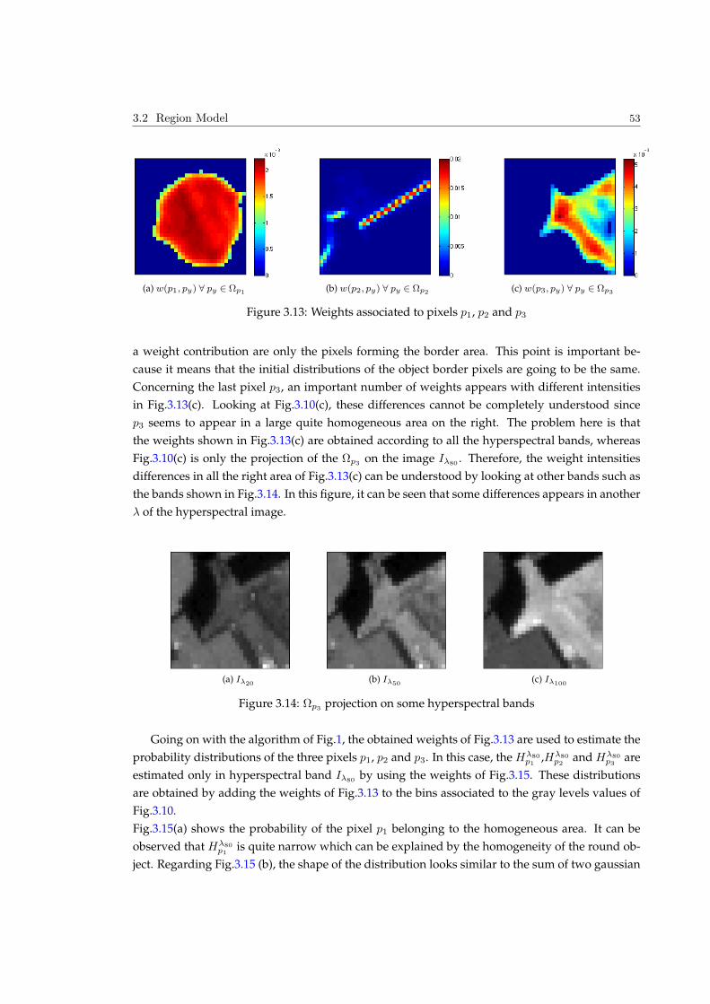
3.2 Region Model 53
(a) w(p1, py) ∀ py ∈ Ωp1 (b) w(p2, py) ∀ py ∈ Ωp2 (c) w(p3, py) ∀ py ∈ Ωp3
Figure 3.13: Weights associated to pixels p1, p2 and p3
a weight contribution are only the pixels forming the border area. This point is important be-
cause it means that the initial distributions of the object border pixels are going to be the same.
Concerning the last pixel p3, an important number of weights appears with different intensities
in Fig.3.13(c). Looking at Fig.3.10(c), these differences cannot be completely understood since
p3 seems to appear in a large quite homogeneous area on the right. The problem here is that
the weights shown in Fig.3.13(c) are obtained according to all the hyperspectral bands, whereas
Fig.3.10(c) is only the projection of the Ωp3on the image Iλ80
. Therefore, the weight intensities
differences in all the right area of Fig.3.13(c) can be understood by looking at other bands such as
the bands shown in Fig.3.14. In this figure, it can be seen that some differences appears in another
λ of the hyperspectral image.
(a) Iλ20(b) Iλ50
(c) Iλ100
Figure 3.14: Ωp3projection on some hyperspectral bands
Going on with the algorithm of Fig.1, the obtained weights of Fig.3.13 are used to estimate the
probability distributions of the three pixels p1, p2 and p3. In this case, the Hλ80p1
,Hλ80p2
and Hλ80p3
are
estimated only in hyperspectral band Iλ80by using the weights of Fig.3.15. These distributions
are obtained by adding the weights of Fig.3.13 to the bins associated to the gray levels values of
Fig.3.10.
Fig.3.15(a) shows the probability of the pixel p1 belonging to the homogeneous area. It can be
observed that Hλ80p1
is quite narrow which can be explained by the homogeneity of the round ob-
ject. Regarding Fig.3.15 (b), the shape of the distribution looks similar to the sum of two gaussian

54 Chapter 3. BPT construction
distributions centered around two values. This can be interpreted by the border position of this
pixel p2 situated between two different regions. For the last distribution Hλ80p3
, a maximum of prob-
ability is observed around the value 80. Note that this is explained because the value of p3 in Iλ80
is equal to 82.
0 50 100 150 200 2500
0.05
0.1
0.15
0.2
0 50 100 150 200 2500
0.02
0.04
0.06
0.08
0 50 100 150 200 2500
0.05
0.1
0.15
0.2
(a) Hλ80p1 (b) Hλ80
p2 (c) Hλ80p3
Figure 3.15: Probability distributions associated to weights of Fig.3.13 in Iλ80
At this point, two different region models have been presented for modeling a hyperspectral
region in this section. Thus, different merging criteria are going to be studied in the following
according to these models.
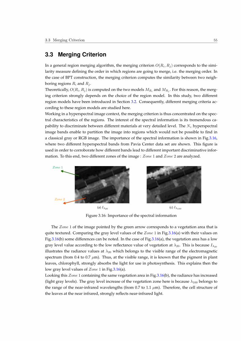
3.3 Merging Criterion 55
3.3 Merging Criterion
In a general region merging algorithm, the merging criterion O(Ri, Rj) corresponds to the simi-
larity measure defining the order in which regions are going to merge, i.e. the merging order. In
the case of BPT construction, the merging criterion computes the similarity between two neigh-
boring regions Ri and Rj .
Theoretically, O(Ri, Rj) is computed on the two models MRiand MRj
. For this reason, the merg-
ing criterion strongly depends on the choice of the region model. In this study, two different
region models have been introduced in Section 3.2. Consequently, different merging criteria ac-
cording to these region models are studied here.
Working in a hyperspectral image context, the merging criterion is thus concentrated on the spec-
tral characteristics of the regions. The interest of the spectral information is its tremendous ca-
pability to discriminate between different materials at very detailed level. The Nz hyperspectral
image bands enable to partition the image into regions which would not be possible to find in
a classical gray or RGB image. The importance of the spectral information is shown in Fig.3.16,
where two different hyperspectral bands from Pavia Center data set are shown. This figure is
used in order to corroborate how different bands lead to different important discriminative infor-
mation. To this end, two different zones of the image : Zone 1 and Zone 2 are analyzed.
(a) Iλ20(c) Iλ100
Zone 1
Zone 2
Figure 3.16: Importance of the spectral information
The Zone 1 of the image pointed by the green arrow corresponds to a vegetation area that is
quite textured. Comparing the gray level values of the Zone 1 in Fig.3.16(a) with their values on
Fig.3.16(b) some differences can be noted. In the case of Fig.3.16(a), the vegetation area has a low
gray level value according to the low reflectance value of vegetation at λ20. This is because Iλ20
illustrates the radiance values at λ20 which belongs to the visible range of the electromagnetic
spectrum (from 0.4 to 0.7 µm). Thus, at the visible range, it is known that the pigment in plant
leaves, chlorophyll, strongly absorbs the light for use in photosynthesis. This explains then the
low gray level values of Zone 1 in Fig.3.16(a).
Looking this Zone 1 containing the same vegetation area in Fig.3.16(b), the radiance has increased
(light gray levels). The gray level increase of the vegetation zone here is because λ100 belongs to
the range of the near-infrared wavelengths (from 0.7 to 1.1 µm). Therefore, the cell structure of
the leaves at the near infrared, strongly reflects near-infrared light.
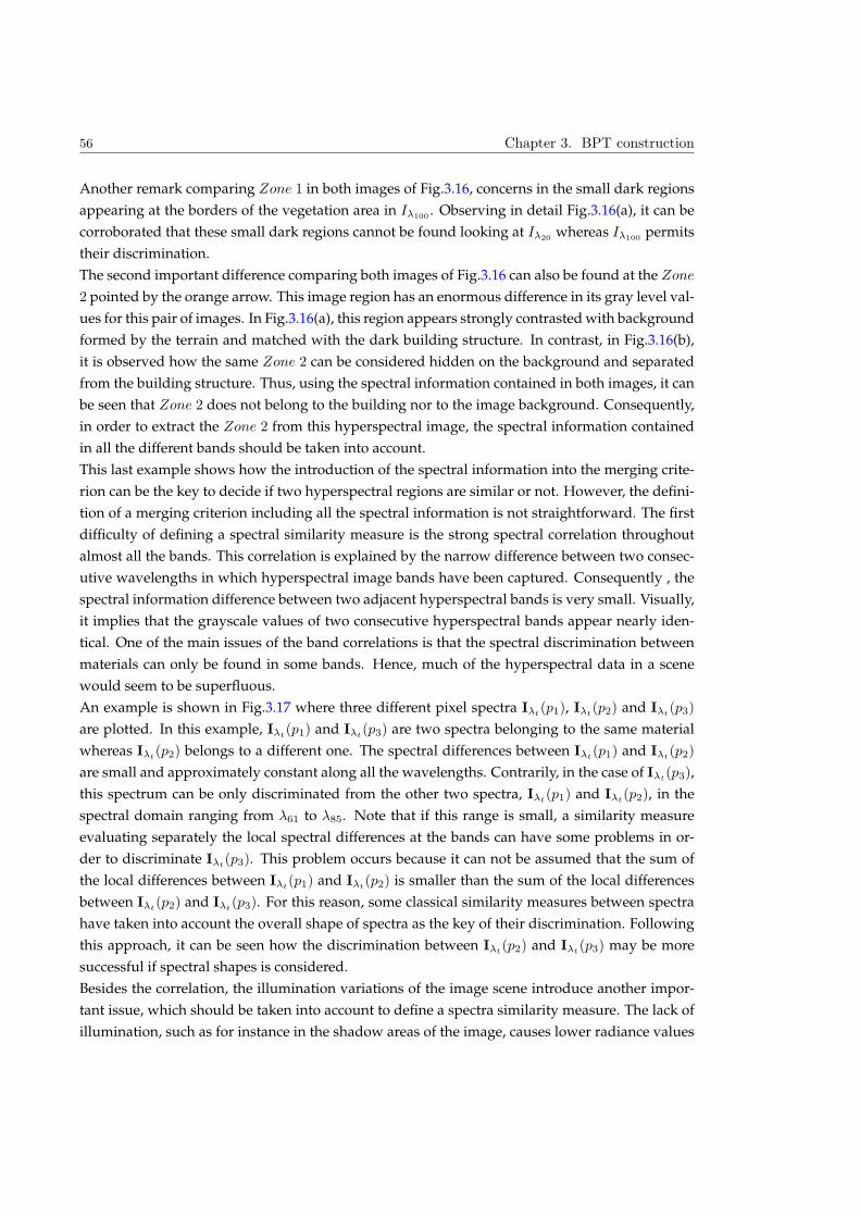
56 Chapter 3. BPT construction
Another remark comparing Zone 1 in both images of Fig.3.16, concerns in the small dark regions
appearing at the borders of the vegetation area in Iλ100. Observing in detail Fig.3.16(a), it can be
corroborated that these small dark regions cannot be found looking at Iλ20whereas Iλ100
permits
their discrimination.
The second important difference comparing both images of Fig.3.16 can also be found at the Zone
2 pointed by the orange arrow. This image region has an enormous difference in its gray level val-
ues for this pair of images. In Fig.3.16(a), this region appears strongly contrasted with background
formed by the terrain and matched with the dark building structure. In contrast, in Fig.3.16(b),
it is observed how the same Zone 2 can be considered hidden on the background and separated
from the building structure. Thus, using the spectral information contained in both images, it can
be seen that Zone 2 does not belong to the building nor to the image background. Consequently,
in order to extract the Zone 2 from this hyperspectral image, the spectral information contained
in all the different bands should be taken into account.
This last example shows how the introduction of the spectral information into the merging crite-
rion can be the key to decide if two hyperspectral regions are similar or not. However, the defini-
tion of a merging criterion including all the spectral information is not straightforward. The first
difficulty of defining a spectral similarity measure is the strong spectral correlation throughout
almost all the bands. This correlation is explained by the narrow difference between two consec-
utive wavelengths in which hyperspectral image bands have been captured. Consequently , the
spectral information difference between two adjacent hyperspectral bands is very small. Visually,
it implies that the grayscale values of two consecutive hyperspectral bands appear nearly iden-
tical. One of the main issues of the band correlations is that the spectral discrimination between
materials can only be found in some bands. Hence, much of the hyperspectral data in a scene
would seem to be superfluous.
An example is shown in Fig.3.17 where three different pixel spectra Iλt(p1), Iλt
(p2) and Iλt(p3)
are plotted. In this example, Iλt(p1) and Iλt
(p3) are two spectra belonging to the same material
whereas Iλt(p2) belongs to a different one. The spectral differences between Iλt
(p1) and Iλt(p2)
are small and approximately constant along all the wavelengths. Contrarily, in the case of Iλt(p3),
this spectrum can be only discriminated from the other two spectra, Iλt(p1) and Iλt
(p2), in the
spectral domain ranging from λ61 to λ85. Note that if this range is small, a similarity measure
evaluating separately the local spectral differences at the bands can have some problems in or-
der to discriminate Iλt(p3). This problem occurs because it can not be assumed that the sum of
the local differences between Iλt(p1) and Iλt
(p2) is smaller than the sum of the local differences
between Iλt(p2) and Iλt
(p3). For this reason, some classical similarity measures between spectra
have taken into account the overall shape of spectra as the key of their discrimination. Following
this approach, it can be seen how the discrimination between Iλt(p2) and Iλt
(p3) may be more
successful if spectral shapes is considered.
Besides the correlation, the illumination variations of the image scene introduce another impor-
tant issue, which should be taken into account to define a spectra similarity measure. The lack of
illumination, such as for instance in the shadow areas of the image, causes lower radiance values
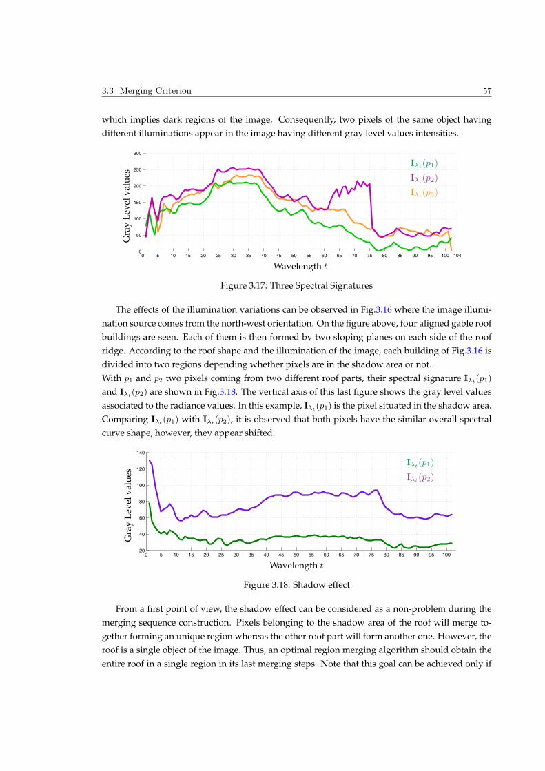
3.3 Merging Criterion 57
which implies dark regions of the image. Consequently, two pixels of the same object having
different illuminations appear in the image having different gray level values intensities.
0 5 10 15 20 25 30 35 40 45 50 55 60 65 70 75 80 85 90 95 100 1040
50
100
150
200
250
300
Wavelength t
Gra
yL
evel
val
ues
Iλt(p1)
Iλt(p2)
Iλt(p3)
Figure 3.17: Three Spectral Signatures
The effects of the illumination variations can be observed in Fig.3.16 where the image illumi-
nation source comes from the north-west orientation. On the figure above, four aligned gable roof
buildings are seen. Each of them is then formed by two sloping planes on each side of the roof
ridge. According to the roof shape and the illumination of the image, each building of Fig.3.16 is
divided into two regions depending whether pixels are in the shadow area or not.
With p1 and p2 two pixels coming from two different roof parts, their spectral signature Iλt(p1)
and Iλt(p2) are shown in Fig.3.18. The vertical axis of this last figure shows the gray level values
associated to the radiance values. In this example, Iλt(p1) is the pixel situated in the shadow area.
Comparing Iλt(p1) with Iλt
(p2), it is observed that both pixels have the similar overall spectral
curve shape, however, they appear shifted.
0 5 10 15 20 25 30 35 40 45 50 55 60 65 70 75 80 85 90 95 10020
40
60
80
100
120
140
Wavelength t
Gra
yL
evel
val
ues
Iλt(p1)
Iλt(p2)
Figure 3.18: Shadow effect
From a first point of view, the shadow effect can be considered as a non-problem during the
merging sequence construction. Pixels belonging to the shadow area of the roof will merge to-
gether forming an unique region whereas the other roof part will form another one. However, the
roof is a single object of the image. Thus, an optimal region merging algorithm should obtain the
entire roof in a single region in its last merging steps. Note that this goal can be achieved only if
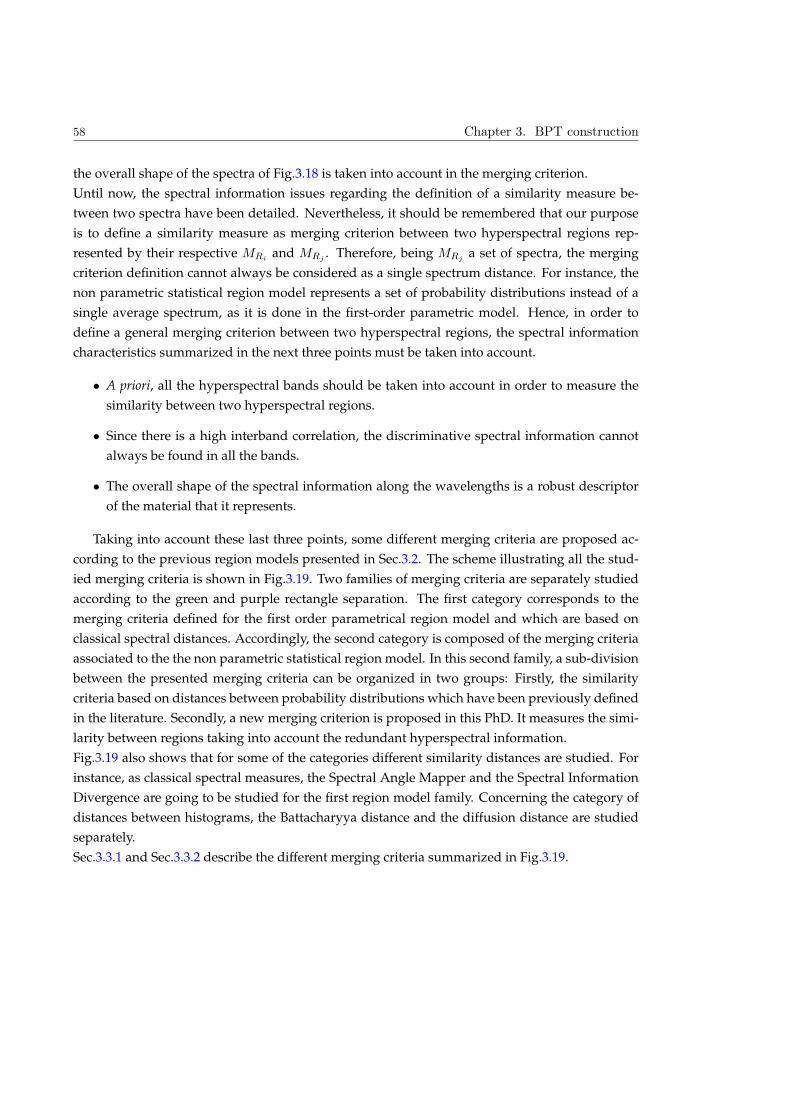
58 Chapter 3. BPT construction
the overall shape of the spectra of Fig.3.18 is taken into account in the merging criterion.
Until now, the spectral information issues regarding the definition of a similarity measure be-
tween two spectra have been detailed. Nevertheless, it should be remembered that our purpose
is to define a similarity measure as merging criterion between two hyperspectral regions rep-
resented by their respective MRiand MRj
. Therefore, being MRja set of spectra, the merging
criterion definition cannot always be considered as a single spectrum distance. For instance, the
non parametric statistical region model represents a set of probability distributions instead of a
single average spectrum, as it is done in the first-order parametric model. Hence, in order to
define a general merging criterion between two hyperspectral regions, the spectral information
characteristics summarized in the next three points must be taken into account.
• A priori, all the hyperspectral bands should be taken into account in order to measure the
similarity between two hyperspectral regions.
• Since there is a high interband correlation, the discriminative spectral information cannot
always be found in all the bands.
• The overall shape of the spectral information along the wavelengths is a robust descriptor
of the material that it represents.
Taking into account these last three points, some different merging criteria are proposed ac-
cording to the previous region models presented in Sec.3.2. The scheme illustrating all the stud-
ied merging criteria is shown in Fig.3.19. Two families of merging criteria are separately studied
according to the green and purple rectangle separation. The first category corresponds to the
merging criteria defined for the first order parametrical region model and which are based on
classical spectral distances. Accordingly, the second category is composed of the merging criteria
associated to the the non parametric statistical region model. In this second family, a sub-division
between the presented merging criteria can be organized in two groups: Firstly, the similarity
criteria based on distances between probability distributions which have been previously defined
in the literature. Secondly, a new merging criterion is proposed in this PhD. It measures the simi-
larity between regions taking into account the redundant hyperspectral information.
Fig.3.19 also shows that for some of the categories different similarity distances are studied. For
instance, as classical spectral measures, the Spectral Angle Mapper and the Spectral Information
Divergence are going to be studied for the first region model family. Concerning the category of
distances between histograms, the Battacharyya distance and the diffusion distance are studied
separately.
Sec.3.3.1 and Sec.3.3.2 describe the different merging criteria summarized in Fig.3.19.
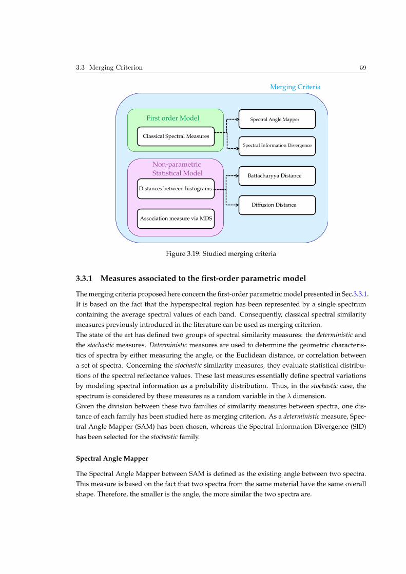
3.3 Merging Criterion 59
First order Model Spectral Angle Mapper
Classical Spectral Measures
Spectral Information Divergence
Battacharyya Distance
Diffusion Distance
Distances between histograms
Association measure via MDS
Non-parametric
Statistical Model
Merging Criteria
Figure 3.19: Studied merging criteria
3.3.1 Measures associated to the first-order parametric model
The merging criteria proposed here concern the first-order parametric model presented in Sec.3.3.1.
It is based on the fact that the hyperspectral region has been represented by a single spectrum
containing the average spectral values of each band. Consequently, classical spectral similarity
measures previously introduced in the literature can be used as merging criterion.
The state of the art has defined two groups of spectral similarity measures: the deterministic and
the stochastic measures. Deterministic measures are used to determine the geometric characteris-
tics of spectra by either measuring the angle, or the Euclidean distance, or correlation between
a set of spectra. Concerning the stochastic similarity measures, they evaluate statistical distribu-
tions of the spectral reflectance values. These last measures essentially define spectral variations
by modeling spectral information as a probability distribution. Thus, in the stochastic case, the
spectrum is considered by these measures as a random variable in the λ dimension.
Given the division between these two families of similarity measures between spectra, one dis-
tance of each family has been studied here as merging criterion. As a deterministic measure, Spec-
tral Angle Mapper (SAM) has been chosen, whereas the Spectral Information Divergence (SID)
has been selected for the stochastic family.
Spectral Angle Mapper
The Spectral Angle Mapper between SAM is defined as the existing angle between two spectra.
This measure is based on the fact that two spectra from the same material have the same overall
shape. Therefore, the smaller is the angle, the more similar the two spectra are.
60 Chapter 3. BPT construction
Given two region models MRiand MRj
representing two adjacent regions by their mean spectra
IRλ and IRλ , the use of SAM as merging criterion is given by
OSAM = argminRi,Rj
cos−1
0
BBBBBB@
NzX
z=1
IRi
λzIRj
λz
vuut
NzX
z=1
IRi
λzIRi
λz
NzX
z=1
IRj
λzIRj
λz
1
CCCCCCA
(3.8)
Note that this spectral angle is relatively insensitive to changes in pixel illumination because
increasing or decreasing illumination does not change the direction of the vector, only its magni-
tude (See Fig.3.18). This insensitivity to the illumination variations is also found in the Spectral
Information Divergence which is studied as the second similarity measure.
Spectral Information Divergence
The Spectral Information Divergence computes the probabilistic discrepancy between two spec-
tral signatures modeled by their corresponding probability distributions PRi(λ) and PRj
(λ). The
use of the SID as merging criterion then implies that the probability distribution PR(λ) associated
to each MR should be computed as a first step. To address the modelling of MR as a random
variable in the λ dimension, the spectrum normalization of Eq. 3.9 is applied at each λi
PR(λi) = IRλi/
NzX
t=1
IRλt(3.9)
where IRλicorresponds to the average of the values of all spectra p 2 R in each band λi.
The estimation of PRi(λ) and PRj
(λ) enables the computation of a similarity measure between
Ri and Rj by computing the Kullback Leibler divergence D(Ri, Rj) between their probability
distributions as follows:
D(Ri, Rj) =
NX
k=1
PRi(λk) logPRi(λk)
PRj(λk)(3.10)
Note that this measure is not symmetric, therefore, the dual divergence must be computed in
order to use D(Ri, Rj) as merging criterion. Finally, the merging criterion by using the Spectral
Information Divergence is given by
OSID = argminRi,Rj
D(Ri, Rj) + D(Rj , Ri) (3.11)
3.3 Merging Criterion 61
3.3.2 Measures associated to the non parametrical statistical region model
In the case of non parametrical statistical region model, a region is represented by a set of spatial
histograms. Each histogram corresponds to the distribution of the radiance intensities at each
wavelength. Given this region model, distances between histograms are studied here.
In image processing, it is well known that the design of a robust histogram distance is a chal-
lenging task because histograms are quite sensitive to changes such as the quantization effects. In
the literature, two families of distances have been defined according to the type of bin correspon-
dence: the classical bin-to-bin and the cross-bin distances. In the first group, distances just compare
each bin in one histogram to the corresponding bin in the other. Some classical examples belong-
ing to this category are the Minkowski distance (such as L1 and L2), the histogram intersection,
the Kullback-Leibler metric, or the Bhattacharyya distance. The second family corresponds to
the cross-bin distances allowing the cross-bin comparison. Consequently, this second family of
distances is more robust to distortions. The Earth Mover’s Distance (EMD)[60] and Diffusion dis-
tance [59] fall into this second category.
In this work, one distance of each family has been studied as merging criterion. Concerning the
bin-to-bin distances, Battacharyya distance has been chosen to be studied. In the same context,
this measure has been previously proposed and tested in [17] its effectiveness has been demon-
strated compared to other distances such as the Kullback-Leibler metric. In the case of cross-bin
distances, diffusion distance has been chosen due to its fast computation time compared to other
measures.
These two classical distances are proposed in this section as merging criteria. Note that these
distances are measured separately for each band. Accordingly, the correlation between the his-
tograms in the spectral domain has not been taken into account by these distances. Hence, another
merging criterion has been defined for the non parametrical statistical region model. The idea of
this third merging criterion is to exploit the properties of the spectral information explained at the
beginning of this section. To this end, it involves two steps for each pair of adjacent regions: 1) the
extraction of the discriminative information contained in each region and 2) the definition of an
association measure measuring the similarity between the information obtained in the first step.
This last merging criterion has been called here as the association measure via Multidimensional
Scaling (MDS). In the following, the three merging criterion are detailed.
Battacharyya Distance
The bin-to-bin Bhattacharyya distance between two statistical discrete distributions measures the
amount of overlap between them. Given two adjacent regions Ri and Rj , modeled by their non
parametrical statistical region models, the Battacharyya distance at band λk between the distribu-
tions Hλk
Riand Hλk
Rj. is defined by
BC(Hλk
Ri, Hλk
Rj) = − log(
NBinsX
s=1
Hλk
Ri(as)
12Hλk
Rj(as)
12 ) (3.12)
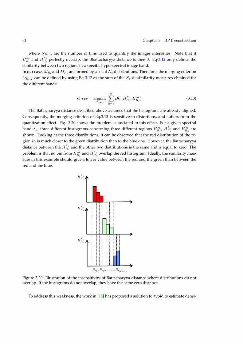
62 Chapter 3. BPT construction
where NBins are the number of bins used to quantify the images intensities. Note that if
Hλk
Riand Hλk
Rjperfectly overlap, the Bhattacharyya distance is then 0. Eq-3.12 only defines the
similarity between two regions in a specific hyperspectral image band.
In our case, MRiand MRj
are formed by a set of Nz distributions. Therefore, the merging criterion
OBAT can be defined by using Eq-3.12 as the sum of the Nz dissimilarity measures obtained for
the different bands:
OBAT = argminRi,Rj
NX
k=1
BC(Hλk
Ri, Hλk
Rj) (3.13)
The Battacharyya distance described above assumes that the histograms are already aligned.
Consequently, the merging criterion of Eq.3.13 is sensitive to distortions, and suffers from the
quantization effect. Fig. 3.20 shows the problems associated to this effect. For a given spectral
band λk, three different histograms concerning three different regions Hλk
Ri, Hλk
Rjand Hλk
Rpare
shown. Looking at the three distributions, it can be observed that the red distribution of the re-
gion Ri is much closer to the green distribution than to the blue one. However, the Battacharyya
distance between the Hλk
Riand the other two distributions is the same and is equal to zero. The
problem is that no bin from Hλk
Rjand Hλk
Rpoverlap the red histogram. Ideally, the similarity mea-
sure in this example should give a lower value between the red and the green than between the
red and the blue.
Pa1 , Pa2 , .........PaNbins
HλkRi
HλkRj
HλkRp
Figure 3.20: Illustration of the insensitivity of Battacharyya distance where distributions do notoverlap. If the histograms do not overlap, they have the same zero distance
To address this weakness, the work in [18] has proposed a solution to avoid to estimate densi-
3.3 Merging Criterion 63
ties formed by too many bins with zero probability which, in practice, may decrease the value of
the similarity measure between the densities. The solution consists in convolving the histograms
by a triangular window. Note that this approach introduces some probability values that are
not really existing in the region. Therefore, in order to solve this problem, the work presented
here has proposed the use of a cross-bin measure between probability distributions as a solution.
Thus, the diffusion distance is proposed as a cross-bin similarity measure [59] in the following. It
defines a second merging criterion.
Diffusion Distance
The diffusion distance DK is a cross-bin distance defined to measure the similarity between two
discrete probability distributions, which cannot be overlapped. The main idea of this distance is
to measure the difference between two histograms at various resolution scales through a diffusion
process. Therefore, the goal is to measure at the different scales how the histogram are different.
If the histograms are different, the difference between them will exist in several scales.
The diffusion process is computed by convolving the histogram difference dl(as) with a Gaussian
filter φσG(as) ,where as 2 Rm is a vector. Thus, each diffusion scale l is computed by a convolution
task and a downsampling step as:
d0(as) = Hλk
Ri(as)−Hλk
Rj(as) (3.14)
dl(as) = [dl−1(as) φσG(as)] #2 l 2 [1, ..., L] (3.15)
The notation #2 denotes downsampling by a factor of two. L is the number of pyramid layers
and σG is the constant standard deviation for the Gaussian filter φ. From the Gaussian pyramid
constructed by Eq.3.15, a distance DK between the histograms can be computed summing up the
L1 norms of the various levels:
DK(Hλk
Ri, Hλk
Rj) =
LX
l=0
NBX
s=1
|dl(as)| (3.16)
Consequently, the proposed merging criterion using the diffusion distance defined in previous
equations is derived as:
ODIF = argminRi,Rj
NX
k=1
DK(Hλk
Ri, Hλk
Rj) (3.17)
Before concluding on merging criteria using classical histogram distances, it should be re-
membered that hyperspectral bands are processed separately by the last two criteria: OBAT and
ODIF . As a result, the correlation between bands is not taken into account in these merging cri-
teria. Moreover, the overall spectral shape of the spectra is another unused information. Note
that in order to include all of these notions, the non parametric statistical region model should be
processed entirely. Ideally, this could be done if the region model was the full multidimensional
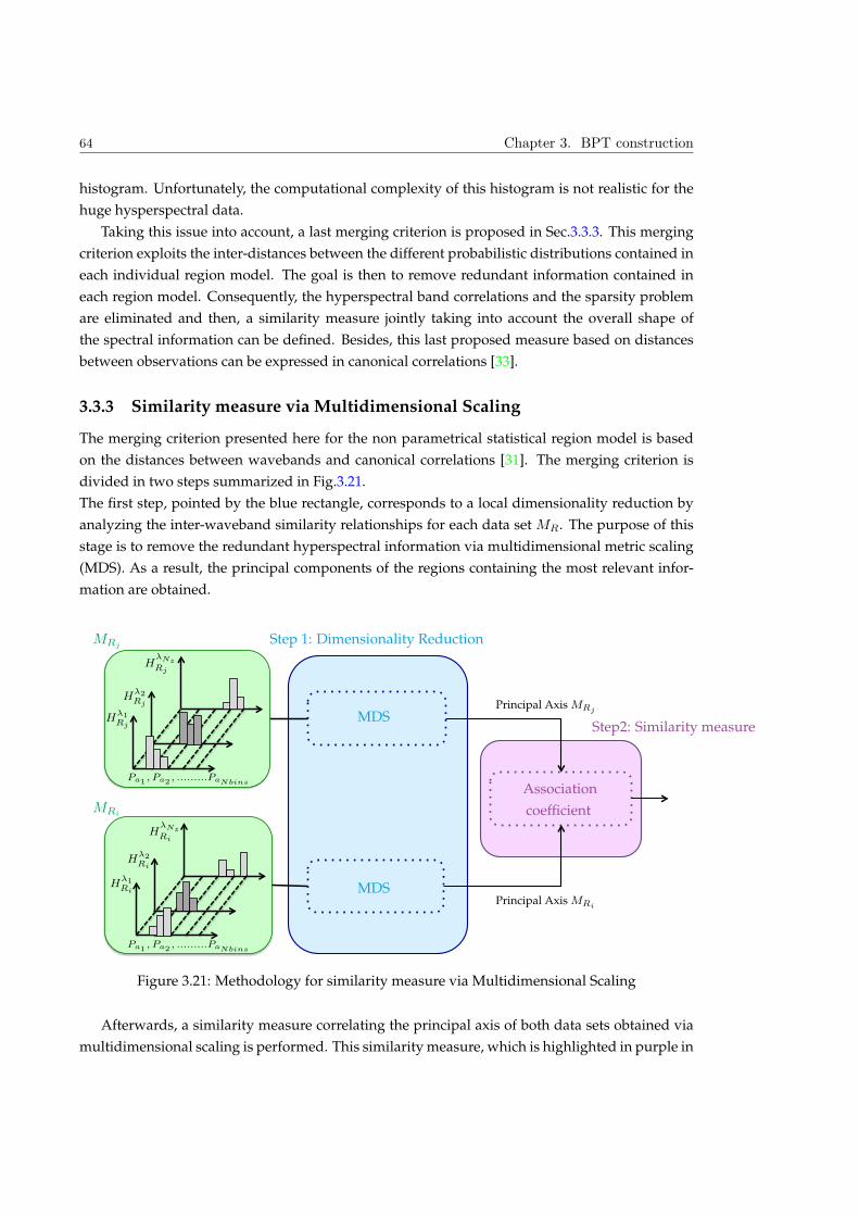
64 Chapter 3. BPT construction
histogram. Unfortunately, the computational complexity of this histogram is not realistic for the
huge hysperspectral data.
Taking this issue into account, a last merging criterion is proposed in Sec.3.3.3. This merging
criterion exploits the inter-distances between the different probabilistic distributions contained in
each individual region model. The goal is then to remove redundant information contained in
each region model. Consequently, the hyperspectral band correlations and the sparsity problem
are eliminated and then, a similarity measure jointly taking into account the overall shape of
the spectral information can be defined. Besides, this last proposed measure based on distances
between observations can be expressed in canonical correlations [33].
3.3.3 Similarity measure via Multidimensional Scaling
The merging criterion presented here for the non parametrical statistical region model is based
on the distances between wavebands and canonical correlations [31]. The merging criterion is
divided in two steps summarized in Fig.3.21.
The first step, pointed by the blue rectangle, corresponds to a local dimensionality reduction by
analyzing the inter-waveband similarity relationships for each data set MR. The purpose of this
stage is to remove the redundant hyperspectral information via multidimensional metric scaling
(MDS). As a result, the principal components of the regions containing the most relevant infor-
mation are obtained.
MRi
Pa1 , Pa2 , .........PaNbins
Hλ2Ri
HλNzRi
Hλ1Ri
MRjStep 1: Dimensionality Reduction
Step2: Similarity measure
Association
coefficient
Pa1, Pa2
, .........PaNbins
Hλ2Rj
HλNzRj
Hλ1Rj
Principal Axis MRj
Principal Axis MRi
MDS
MDS
Figure 3.21: Methodology for similarity measure via Multidimensional Scaling
Afterwards, a similarity measure correlating the principal axis of both data sets obtained via
multidimensional scaling is performed. This similarity measure, which is highlighted in purple in
3.3 Merging Criterion 65
Fig.3.21, relies on a statistical test based on the multivariate analysis of variance (MANOVA). The
goal is to test whether there is a dependence (or correlation) between the principal components
of the regions or not.
Step1: Dimensionality Reduction
Multidimensional scaling (MDS) [28] represents a set of objects as a set of points in a map of cho-
sen dimensionality, based on their interpoint distances. The objective is to maximize the agree-
ment between the displayed interpoint distances and the given ones. Thus, MDS attempts to
locate No objects as points in an Euclidean space E where the geometric differences between
pairs of points in E agree, as closely as possible, with the true differences between the No objects.
In our case, the No objects correspond to the Nz probability distributions of each MR. Hence, the
probability distribution similarities (or dissimilarities) of MR can be represented by a Nz x Nz dis-
tance matrix ∆R= (δkl), where δkl = δlk ≥0 is the diffusion distance value computed by Eq. 3.16.
Hence, being A the matrix with entries A = −( 12 )δ2kl and the centering matrix H = IN − 1
N11t ,
the so-called inner product matrix BR associated to ∆R can be computed by BR = HAH for each
MR [28]. BR is also called Gower’s centered matrix which is computed by centering the elements
of A [32].
The inner product matrix BR is an NzxNz symmetric matrix which can be spectrally decomposed
as BR = URΛ2RU
tR. Assuming that the eigenvalues in Λ2
R are arranged in descending order, the
matrix URΛR and UR contains the principal and the standard coordinates of region R, respec-
tively.
As mentioned above, the aim of MDS is to represent MR in a lower dimensional space, by tak-
ing the first Ds most representative principal or standard coordinates. Therefore, given two
regions defined by MRiand MRj
, this first step computes the first Ds standard coordinates of
MRiand MRj
. That is, two distance matrices ∆Riand ∆Rj
to find BRi= URi
Λ2RiU tRi
and
BRj= URj
Λ2Rj
U tRj
are computed using the explained procedure.
Selection of the number of dimension Ds
The number of dimensions Ds is an important aspect in most multivariate analysis methods.
Classically, the number of dimensions is based on the percentage of variability accounted for
by the first dimensions. Therefore, a popular criterion consists in selecting the first eigenvectors
corresponding to the highest eigenvalues. In this case, the Ds components represent the maximum
possible proportion of the variance in Ds dimensions. Applying this strategy with Nz possible
eigenvalues arranged in descending order, the dimension Ds is then given by Eq.3.18.
DsX
t=1
λtR
NzX
t=1
λtR
1 (3.18)
66 Chapter 3. BPT construction
where λNzR and λ1R correspond to the smallest and the highest eigenvalues, respectively.
This criterion has been the only criterion used in hyperspectral methods performing dimension-
ality reduction techniques as PCA [10] [36] [116]. Note that PCA corresponds to the special case
of multidimensional scaling metric when the euclidean distance is used as δ. For these works, the
criterion according to Eq.3.18 has allowed to extract the first Ds uncorrelated components.
Unfortunately, this criterion can have some issues in our case. The problem is that the Ds prin-
cipal coordinates representing two different regions can be correlated between themselves. For
example, let us consider that Ds is equal to 5 for two neighboring regions which leads to the result
of 5 different eigenvectors. If these 5 eigenvectors give different information, i.e. are uncorrelated,
the choice of Ds is correct. However, if the first eigenvector of the first region is highly correlated
with the fourth component of the second region, the choice of Ds = 5 is going to introduce a bias.
Therefore, it may be better to choose Ds = 3 in this example.
Here, in order to solve the explained limitation, a criterion which extends a sequence c defined
and studied in [33] is used to set the value of Ds. Firstly, a maximum dimension Ns suggested by
the data should be fixed, which corresponds to the minimum dimension for which
PNs
t=1 λ2tR
PNz
t=1 λ2tR
1
(Such as 3.18). Then, with ui and vi, i = 1, ..., Ns, being the Ns first eigenvectors of URiand URj
,
a sequence Ck is defined as:
Ck =
Pk
t=1
Pk
p=1 λ2tRi
(u0tvp)
2λ2tRj
PNs
t=1
PNs
p=1 λ2tRi
(u0tvp)
2λ2tRj
k 2 [1, ..., Ns] (3.19)
where λ2tRi
λ2tRj
are the eigenvalues of BRiand BRj
which are proportional to the variances of
the corresponding principal axes. The term (u0tvp)
2 is the correlation coefficient between the t-th
and the p-th eigenvectors. Thus, the numerator in ck can be interepreted as a weighted average of
the relationships between principal axes.
Clearly 0 C1 , ... CDs, ... CNs
= 1. Hence, the dimension Ds is then chosen such
that CDsis high, for instance CDs
= 0.9. In this way, Ds represents the number of uncorrelated
eigenvectors representing the largest proportion of variance.
Step2: Similarity measure between MRiand MRj
principal axis
The proposed similarity measure relies on measuring the correlation, also called dependency, be-
tween the principal coordinates representing two adjacent regions. This notion of multivariate
dependence test can be easily explained by the next example.
Assume that a study wants to be conducted to evaluate the students’ improvements in math and
physics by trying different textbooks. In that case, improvements in math and physics are the
two dependent variables, and the goal is to test the following hypothesis: Are both topics jointly
affected by the difference in textbooks?
As a result, if the overall multivariate test is significant, it can be concluded that the respective
effect (e.g., textbook) is significant. In our case, changing the textbooks and the improvements by
two different hyperspectral regions, the purpose of the dependence test still remains the same.
3.3 Merging Criterion 67
Hence, the goal is to measure if a multivariate test between two regions defined by their principal
coordinates (URiΛRi
and URjΛRj
) will be significant or not.
It is done by interpreting the Ds columns of URiΛRi
and URjΛRj
as a predictor X and a response
variable Y of a multivariate linear regression model, respectively. Regression analysis helps to an-
alyze such situations by focusing on the change in a dependent variable associated with changes
in two or more independent variables. The expression of this multivariate linear regression model
is given by:
Y = Xβ + e (3.20)
where β is the matrix of parameters containing the regression coefficients and e is the matrix
of residual errors. Given Eq.3.20, the aim is to use this model to test if Y and X are correlated or,
in other words, if Y is a linear combination of X. It is clearly seen that if there is no relationship
between X and Y, the matrix β is equal to 0.
The goal is therefore to measure if a significant relationship between X and Y exists by testing
the multivariate general linear hypothesis β = 0.
The proposed multivariate statistical test is based on the Multivariate analysis of the variance
(MANOVA) theory. The MANOVA has been largely used to measure the interactions among
dependent and independent multidimensional variables. The primary objective is to assess the
significance of group differences. To estimate it, MANOVA studies the covariances of the vari-
ables as well as their individual variances by the sums of squares and cross-products matrices,
which are the basis for these quantities.
The sums of squares and cross-products matrices evaluates how is the residual error e = (Y −Xβ)
measuring the error of the prediction matrix Y according to Y . The prediction matrix Y = Xβ
is defined by the estimation of the regression coefficients β. In the case of multivariate data, the
simplest method to estimate the matrix β is the ordinary least-squares method which minimizes
the sum of squares residuals tr(e0e) = tr[(Y − Xβ)t(Y − Xβ)] [30]. The least-squares solution
for β estimation is given by β = (XtX)−1XtY . Accordingly, the prediction matrix is given by
Y = Xβ = PY where P = X(XtX)−1Xt is the known hat matrix [34].
The regression equation allows to find the score of an outcome, and these scores are such that
Y = Y + e, so the Total Sum of Square and Cross Product SSCP is given as:
Y tY = (Y + e)t(Y + e)
= Y tY + Y te+ etY + ete
= Y tY + ete (3.21)
Eq. 3.21 shows how SSCP is decomposed into Sum of Square and Cross Product of scores of
outcomes Y tY and Sum of Square and Cross Product of errors ete. These two matrices denoted
in the following by H and E summarize the (co)variation of the fitted values and residuals for
a given predictor Y . In MANOVA theory, they have been used to define different multivariate
68 Chapter 3. BPT construction
dependences test to verify the general linear hypothesis β = 0.
The most common multivariate statistic test to measure if the hypothesis β = 0 is true or false is
known as Wilks’ lambda likelihood ratio test W . Besides this test, it must be remarked that other
multivariate statistics tests as Roy, Lawley-Hotteling or Pillai criteria to test β = 0 have been
studied.(See Appendix 6.3 for further information). Also, association measures without consid-
ering the multivariate regression model have also been taken into account as measures shown in
Appendix 6.3. Comparing all these measures, Wilks’ lambda test has been chosen because the
association measure obtained by Wilks’ lambda test Aw leads to the highest value of association.
It means that the other measures can obtain very small values which could be interpreted as a
null association.(See order relationship in Appendix.6.3).
The Wilks’ lambda test can be interpreted as the proportion of generalized variance in the depen-
dent variables that is accounted for by the predictors. This treatment is performed by finding the
ratio of the determinant (generalized variance) of the error SSCP matrix to the determinant of the
sum of the treatment and error E matrices. Mathematically, the Wilks’ lambda W is expressed by:
W (X,Y ) =det(E)
det(E +H)=
det(ete)
det(Y tY )(3.22)
where the term ete is defined by:
ete = (Y −Xβ)t(Y −Xβ)
= Y tY − Y tXβ − βXtY + βtXtY + βtXtXβ
= Y tY − Y tXβ ( where βtXtY = βtXtXβ )
= Y tY − Y tX(XtX)−Y
= Y 0[I −X(XtX)−Xt]Y (3.23)
The Wilks’ lambda test satisfies 0 W (X,Y ) 1 . The zero value indicates that the hypothesis
β = 0 is false and then X and Y are highly correlated. Contrarily, if W (X,Y ) = 1, the hypothesis
is true and then X and Y are completely independent. It must be remembered that in our case,
X and Y correspond to the principal coordinates of the region represented by Y = URjΛRj
and
X = URiΛRi
. The predicted model Y then corresponds to
Y = PY = X(XtX)−1XtY = URiU 0RiURj
ΛRj(3.24)
Hence, given Eq. 3.23 and Eq.3.24, the Sum of Square and Cross Product of errors E and the
total Sum of Square and Cross Product E+H are given by:
E = ete = Y 0[I −X(XtX)−Xt]Y = ΛRj(I − U t
RjURi
U tRiURj
)ΛRj(3.25)
E +H = Y tY = ΛRjU tRj
URjΛRj
= Λ2Rj
(3.26)
3.3 Merging Criterion 69
These last two expressions re-define the Wilks’ lambda test of Eq.3.22. In this context, X and
Y correspond to region models representing two adjacent regions Ri and Rj . Accordingly, the
Wilks’ lambda test W (Ri, Rj) is expressed by Eq.3.27. This last equation can be used to define an
association measure as Aw = 1−W , which does not depend on ΛRjneither ΛRi
.
W (Ri, Rj) = det(I − U tRj
URiU tRiURj
) (3.27)
The Wilks’ lambda test of Eq. 3.22, can also be calculated from the point of view of an eigen-
value approach by W (Ri, Rj) = λ1w λ2
w.... λDsw where λi
w are the eigenvalues corresponding
to:
det(E − λw(E +H)) = 0 (3.28)
with 0 λiw 1. These eigenvalues are directly related to the canonical correlations which
are used as a way of measuring the linear relationship between two multidimensional variables.
In this context, the squared canonical correlation r2i is defined by 1− λiw. The Wilks’ criterion can
thus be expressed in terms of canonical correlations as:
W (Ri, Rj) =
DsY
i=1
(1− r2i ) (3.29)
Hence, the Wilks’ lambda test computed in Eq.3.29 is proposed here as the similarity measure
between Ri and Rj . If W (Ri, Rj) is equal to 0, it means that the hypothesis β = 0 is false and
then Ri and Rj are highly correlated, i.e. very similar. In contrast, W (Ri, Rj) = 1 implies that the
adjacent regions Ri and Rj are very different and no dependency can be found. Hence, this leads
to the definition of the proposed merging criterion:
OMDS = argminRi,Rj
W (Ri, Rj) (3.30)
Before concluding this section, we would like to remark that all the proposed merging criteria
shown in Fig.3.19 are size-independent. In other words, the area of the regions is not included in
any proposed merging order. Thus, depending on the initial partition where the merging process
is started and on the specific characteristics of the image, these approaches may suffer from small
and meaningless regions into the generated partition. This limitation is found especially in the
initial stages of the BPT construction process.
To overcome this issue, the combination of a scale-based merging order with the presented area-
independent merging criteria is used here as it has been previously done in [17]. The benefit of this
approach is that the fusion of large regions is not too penalized compared to classical approaches,
where the area of the region is multiplied by the similarity measure O(Ri, Rj) [40] [141] .
The problem of this approach is that the area constraint and the similarity measure O(Ri, Rj) can
have different magnitude orders. An example can be seen in Eq.3.31 where a weighted merging
criterion has been proposed in [17] by using the Battacharyya distance of Eq.3.13. In this example,
70 Chapter 3. BPT construction
the merging order obtained by the similarity measure is multiplied by the minimum area of the
pair of regions. In this case, OBAT and the area constraint can really have different magnitude
orders. The term OBAT comes from a logarithmic function , it can therefore be much more smaller
than the first term concerning the area of the regions. Hence, this approach can force to obtain
regions having similar sizes by strongly enforcing the area constraint.
OweightedBAT = min(NRip
, NRjp)OBAT (3.31)
To avoid this limitation, the scale-threshold procedure is included during the construction of
BPT in order to avoid meaningless regions at the different levels of the hierarchy.
Introduction of the scale-threshold in the merging criteria
The idea proposed in [17] is to define a scale threshold TLi
scale at each merging step Li according to
the number of remaining regions in the partition. At each step Li, the TLi
scale is considered as the
minimum area that regions forming the partition of this level should have.
The combination of the scale-threshold constraint with the region merging order described on
Fig.3.1 can be easily performed. The strategy consists in verifying for each Li, whether there are
regions of size lower than TLi
scale.
Regions below this threshold are considered as out-of-scale and the algorithm forces their merg-
ing (following their similarity values). It should be noticed that even if the out-of-scale regions
are forced to merge at a given level, they will merge with their most similar neighboring region
in the partition.
The scale threshold is updated after each merging step and its definition is based on the average
size of regions at a certain iteration Li by:
TLi
scale =↵ · Image Area
Number of regions at Li
(3.32)
Note that even if the out-of-scale criterion forces the fusion of the small regions, the constraint
is not too restrictive because it still permits to have small regions different from their neighbor-
hood, at that high levels of the BPT hierarchy. For instance, assuming an image containing 1000
pixels and ↵ = 0.15. After 980 merging steps, the resulting partition at level L980 is formed by
21 different regions can be composed of regions having as few as 8 pixels. Heuristically, a good
trade-off was presented in [17] by using ↵ = 0.15
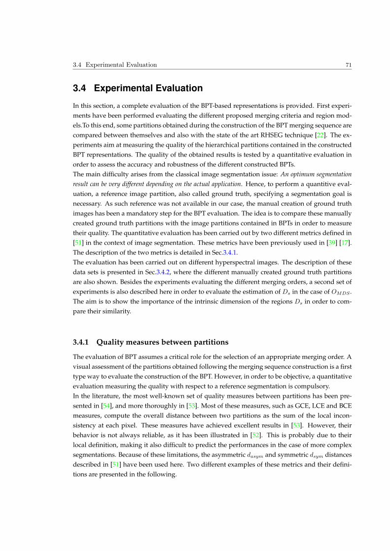
3.4 Experimental Evaluation 71
3.4 Experimental Evaluation
In this section, a complete evaluation of the BPT-based representations is provided. First experi-
ments have been performed evaluating the different proposed merging criteria and region mod-
els.To this end, some partitions obtained during the construction of the BPT merging sequence are
compared between themselves and also with the state of the art RHSEG technique [22]. The ex-
periments aim at measuring the quality of the hierarchical partitions contained in the constructed
BPT representations. The quality of the obtained results is tested by a quantitative evaluation in
order to assess the accuracy and robustness of the different constructed BPTs.
The main difficulty arises from the classical image segmentation issue: An optimum segmentation
result can be very different depending on the actual application. Hence, to perform a quantitive eval-
uation, a reference image partition, also called ground truth, specifying a segmentation goal is
necessary. As such reference was not available in our case, the manual creation of ground truth
images has been a mandatory step for the BPT evaluation. The idea is to compare these manually
created ground truth partitions with the image partitions contained in BPTs in order to measure
their quality. The quantitative evaluation has been carried out by two different metrics defined in
[51] in the context of image segmentation. These metrics have been previously used in [39] [17].
The description of the two metrics is detailed in Sec.3.4.1.
The evaluation has been carried out on different hyperspectral images. The description of these
data sets is presented in Sec.3.4.2, where the different manually created ground truth partitions
are also shown. Besides the experiments evaluating the different merging orders, a second set of
experiments is also described here in order to evaluate the estimation of Ds in the case of OMDS .
The aim is to show the importance of the intrinsic dimension of the regions Ds in order to com-
pare their similarity.
3.4.1 Quality measures between partitions
The evaluation of BPT assumes a critical role for the selection of an appropriate merging order. A
visual assessment of the partitions obtained following the merging sequence construction is a first
type way to evaluate the construction of the BPT. However, in order to be objective, a quantitative
evaluation measuring the quality with respect to a reference segmentation is compulsory.
In the literature, the most well-known set of quality measures between partitions has been pre-
sented in [54], and more thoroughly in [53]. Most of these measures, such as GCE, LCE and BCE
measures, compute the overall distance between two partitions as the sum of the local incon-
sistency at each pixel. These measures have achieved excellent results in [53]. However, their
behavior is not always reliable, as it has been illustrated in [52]. This is probably due to their
local definition, making it also difficult to predict the performances in the case of more complex
segmentations. Because of these limitations, the asymmetric dasym and symmetric dsym distances
described in [51] have been used here. Two different examples of these metrics and their defini-
tions are presented in the following.
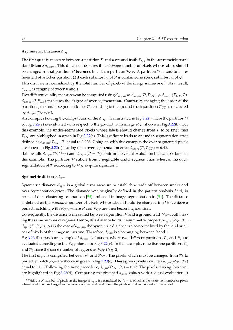
72 Chapter 3. BPT construction
Asymmetric Distance dasym
The first quality measure between a partition P and a ground truth PGT is the asymmetric parti-
tion distance dasym. This distance measures the minimum number of pixels whose labels should
be changed so that partition P becomes finer than partition PGT . A partition P is said to be re-
finement of another partition Q if each subinterval of P is contained in some subinterval of Q.
This distance is normalized by the total number of pixels of the image minus one 1. As a result,
dasym is ranging between 0 and 1.
Two different quality measures can be computed using dasym, as dasym(P,PGT ) 6= dasym(PGT ,P).
dasym(P, PGT ) measures the degree of over-segmentation. Contrarily, changing the order of the
partitions, the under-segmentation of P according to the ground truth partition PGT is measured
by dasym(PGT ,P).
An example showing the computation of the dasym is illustrated in Fig.3.22, where the partition P
of Fig.3.22(a) is evaluated with respect to the ground truth image PGT shown in Fig.3.22(b). For
this example, the under-segmented pixels whose labels should change from P to be finer than
PGT are highligthed in green in Fig.3.22(c). This last figure leads to an under-segmentation error
defined as dasym(PGT ,P) equal to 0.006. Going on with this example, the over-segmented pixels
are shown in Fig.3.22(c) leading to an over-segmentation error dasym(P,PGT ) = 0.42.
Both results dasym(P,PGT ) and dasym(PGT ,P) confirm the visual evaluation that can be done for
this example. The partition P suffers from a negligible under-segmentation whereas the over-
segmentation of P according to PGT is quite significant.
Symmetric distance dsym
Symmetric distance dsym is a global error measure to establish a trade-off between under-and
over-segmentation error. The distance was originally defined in the pattern analysis field, in
terms of data clustering comparison [55] and used in image segmentation in [51]. The distance
is defined as the minimum number of pixels whose labels should be changed in P to achieve a
perfect matching with PGT , where P and PGT are then becoming identical.
Consequently, the distance is measured between a partition P and a ground truth PGT , both hav-
ing the same number of regions. Hence, this distance holds the symmetric property dsym(PGT ,P) =
dsym(P,PGT ). As in the case of dasym, the symmetric distance is also normalized by the total num-
ber of pixels of the image minus one. Therefore, dsym is also ranging between 0 and 1.
Fig.3.23 illustrates an example of dsym evaluation, where two different partitions P1 and P2 are
evaluated according to the PGT shown in Fig.3.22(b). In this example, note that the partitions P1
and P2 have the same number of regions as PGT (NR=2).
The first dsym is computed between P1 and PGT . The pixels which must be changed from P1 to
perfectly match PGT are shown in green in Fig.3.23(c). These green pixels involve a dsym(PGT ,P1)
equal to 0.08. Following the same procedure, dsym(PGT ,P2) = 0.17. The pixels causing this error
are highlighted in Fig.3.23(d). Comparing the obtained dsym values with a visual evaluation, it
1 With the N number of pixels in the image, dasym is normalized by N − 1, which is the maximum number of pixelswhose label may be changed in the worst case, since at least one of the pixels would remain with its own label
3.4 Experimental Evaluation 73
(a) PGT (b) P
(c) Under-segmented pixels (d) Over-segmented pixels
Figure 3.22: Illustrative example of asymmetric partition distance for an image having 10 10pixels. (a) Partition P to be evaluated . (b) Ground truth partition PGT . (c) and (d) are binaryimages showing in green the pixels whose labels must be changed in each case to compute theunder- (dasym(PGT ,P)) and the over-segmentation(dasym(P,PGT )) errors, respectively.
can be seen that both distances provide objective results between the evaluated partitions. Both
evaluations result in the same conclusion, the partition P1 is closer to the ground truth segmenta-
tion than the partition P2.
3.4.2 Data Sets Definition
The experimental evaluation is carried out by using five different hyperspectral images captured
by two different sensors. Accordingly, the different data sets have different spectral and spatial
resolutions. The five hyperspectral images can be split in three categories: three images from
Pavia University, an image from Pavia Center both acquired by the ROSIS sensor and finally, an
image acquired by HYDICE sensor. Five different ground truth partitions have been manually
created.
Due to the low resolution of hyperspectral data, the creation of ground truth partitions is not
straightforward. Therefore, as these images present complex structures, the creation of a com-
plete ground truth is an important challenge. A second important issue is related to the scene
intrepretation. This problem is related with the different information contained in the different
hyperspectral bands. In particular, composing two RGB images by using 6 different hyperspec-
tral bands, two completely different ground truths can be created.
In order to minimize this problem, the RGB image composition used to create the ground truth
partitions has been obtained by the first PCA components. Concretely, it corresponds to the three
74 Chapter 3. BPT construction
(a) P1 (b) P2
(c) dsym(PGT ,P2) = 0.08 (d) dsym(PGT ,P2) = 0.17
Figure 3.23: Illustrative example of symmetric partition distance for an image having 10 10pixels. (a)-(b) Partitions P1 and P2 to be evaluated. (c) and (d) are binary images showing ingreen the pixels whose labels must be changed for partition P1 and P2 to perfectly match withPGT shown in Fig.3.22(b).
components associated to the 3 highest eigenvalues. The generated ground truth partitions and
the characteristics of the five hyperspectral data sets are detailed in the following.
Pavia University
The first studied hyperspectral image is acquired over the city of Pavia (Italy) by the ROSIS− 03
(Reflective Optics Systems Imaging Spectrometer) hyperspectral sensor operated by DLR out of
Oberpfaffenhofen (Germany). The spatial dimension of the image is 610 340. The geometrical
resolution is 1.3 m. The original data are composed of 115 spectral bands, ranging from 0.43 to
0.86 µm with a band width of 4 nm. However, typical noisy bands corresponding to the water
absorption were previously discarded leading to 103 channels. A RGB composition of the entire
Pavia University data set is shown in Fig.3.24.
For this image, the experimental results aiming at the BPT evaluation are not performed by using
the complete image. Indeed, the creation of a ground truth image labeling all the pixels is too
complex. Fig.3.24 shows the complexity of the structures forming this image. Thus, in order to
create an accurate ground truth image, three different portions of hyperspectral Pavia University
have been used. The three different portions studied for the Pavia University data set are boxed
by the red, the orange and the yellow rectangles.
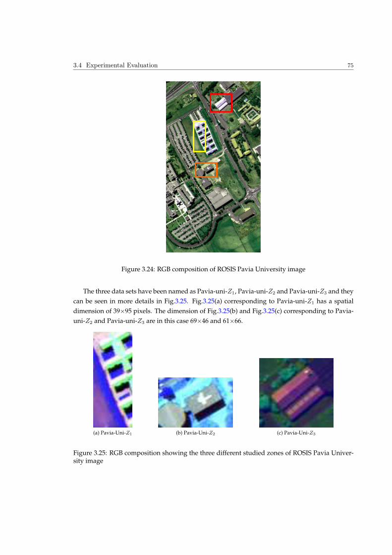
3.4 Experimental Evaluation 75
Figure 3.24: RGB composition of ROSIS Pavia University image
The three data sets have been named as Pavia-uni-Z1, Pavia-uni-Z2 and Pavia-uni-Z3 and they
can be seen in more details in Fig.3.25. Fig.3.25(a) corresponding to Pavia-uni-Z1 has a spatial
dimension of 3995 pixels. The dimension of Fig.3.25(b) and Fig.3.25(c) corresponding to Pavia-
uni-Z2 and Pavia-uni-Z3 are in this case 6946 and 6166.
(a) Pavia-Uni-Z1 (b) Pavia-Uni-Z2 (c) Pavia-Uni-Z3
Figure 3.25: RGB composition showing the three different studied zones of ROSIS Pavia Univer-sity image

76 Chapter 3. BPT construction
For these last images, three manually ground truth partitions PGT have been created. These
reference partitions are shown in Fig.3.26(a)(b)(c). The corresponding numbers of regions NR are
NR = 33, NR = 11 and NR = 42, respectively.
(a) PGT fromPavia-Uni-Z1
(b) PGT from Pavia-Uni-Z2 (c) PGT from Pavia-Uni-Z2
Figure 3.26: Manually created PGT partitions of the three different studied zones of ROSIS PaviaUniversity image
Pavia Center
The second studied hyperspectral data has also been captured by the hyperspectral ROSIS sen-
sor. The entire image has 492 by 1096 pixels, collected over Pavia city centre, Italy. It contains
102 spectral channels after removal of noisy bands. From the same reasons as Pavia University,
a portion of this image has been selected in order to evaluate the BPT construction. The RGB
composition describing the image scene is shown in Fig.3.27(a). The corresponding ground truth
containing NR = 23 regions is shown in Fig.3.27(b).
(a) RGB Composition (b) Manually created PGT
Figure 3.27: Pavia Center Data Set
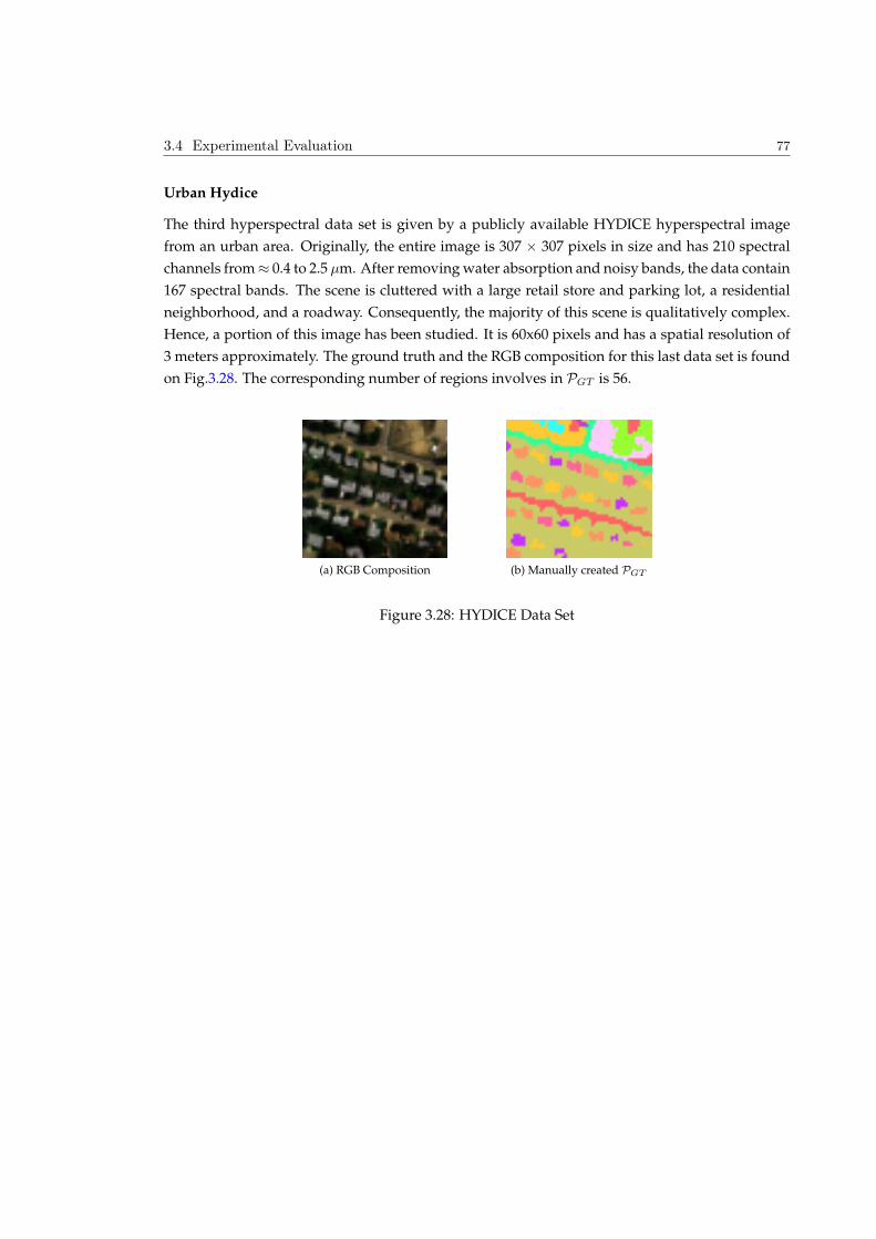
3.4 Experimental Evaluation 77
Urban Hydice
The third hyperspectral data set is given by a publicly available HYDICE hyperspectral image
from an urban area. Originally, the entire image is 307 307 pixels in size and has 210 spectral
channels from 0.4 to 2.5 µm. After removing water absorption and noisy bands, the data contain
167 spectral bands. The scene is cluttered with a large retail store and parking lot, a residential
neighborhood, and a roadway. Consequently, the majority of this scene is qualitatively complex.
Hence, a portion of this image has been studied. It is 60x60 pixels and has a spatial resolution of
3 meters approximately. The ground truth and the RGB composition for this last data set is found
on Fig.3.28. The corresponding number of regions involves in PGT is 56.
(a) RGB Composition (b) Manually created PGT
Figure 3.28: HYDICE Data Set
78 Chapter 3. BPT construction
3.4.3 Experiment 1: Evaluation of BPT hierarchical levels
The purpose of this experiment is to evaluate the different image partitions created during the
BPT construction by the different merging criteria. Starting from the pixel-based representation
of an image containing Np pixels, partitions having a number of regions equal to NR are studied.
These partitions are obtained by doing the Np - NR merging steps over the initial partition. The
quality of the obtained partitions having NR regions is evaluated in two different ways: Visually
and by using the two different partition distances described in Sec.3.4.1.
This complete evaluation is carried out on the five different images presented in Sec.3.4.2. For
each image, different BPTs according to the different merging orders proposed in Fig.3.3 have
been constructed.
To perform this experiment, some parameters for the different region models and merging crite-
ria should be set. In the case of OSID ad OSAM , no parameter is required. Note that the region
model corresponding to these merging orders is only the average of the spectral values of the
region. Contrarily, in order to construct the non parametric statistical region model presented in
Sec.3.3.2, some parameters should be defined. The first important parameter is the number of bins
Nbins used to construct the histogram of each region at each hyperspectral band. Ideally, Nbins
should be equal to the number of possible radiance values contained on the image. For instance,
if the radiance value is an integer encoded over 8 bits, their range is [0, 255]. Therefore, the ideal
number of bins used to represent the spatial histograms of the region corresponds to Nbins = 256.
The main problem is that having hundred of Nz channels, thousands of Np pixels and 2Np − 1
merging steps, a high Nbins value can be computationally critical. On the other hand, radiance
values can also be coded with 16 bits ranging from [0, 65535], therefore, the parameter is even
more critical. Consequently, a moderate quantization is used for the computation of the non
parametric statistical model.
Another consideration concerning Nbins is the possible histogram misalignment problem previ-
ously shown in Fig.3.20. This problem is mainly found because OBAT is not robust with regards
to this point. The robustness of Nbins parameters is sought with the merging order ODIF . For
this criterion, different results can be obtained by changing the value of Nbins, however, their
differences are not very significant. The diffusion distance ODIF needs to set two parameters:
the standard deviation for the Gaussian filter σG and the number of layers. In our work, these
parameters have been set according to [59]. Thus, σG is equal to 0.5 and the number of layers is
set to 3.
Another important parameter concerning the non parametric statistical region model is the value
Ds used in OMDS . The procedure to extract Ds has been explained in Sec.3.3.3. Before conclud-
ing, it should be remembered that other parameters for the case of non parametrical statistical
region model have been defined at the beginning of Sec.3.6. These are the parameters described
to estimate the pdf’s of the individual pixels. In the experiments presented in this section, the
pixel pdf estimation has been performed as it has been previously done on the pixels of Fig.3.10.
At this point, the following sub-sections describe the obtained experimental results for the visual
and quantitive evaluation.
3.4 Experimental Evaluation 79
Visual Evaluation of the hierarchical BPT levels
The visual evaluation of the partitions obtained by the different merging criteria is carried out
here. A set of partitions obtained during the BPT construction having different number of regions
are shown.
Starting from the hyperspectral image illustrated in Fig.3.24, five different BPTs have been con-
structed for each of the three zones: Pavia-uni-Z1 ,Pavia-uni-Z2 and Pavia-uni-Z3. Nbins is set to
120 for these three images and Ds is set to 3.
The first results correspond to the BPT construction for Pavia-uni-Z1, whose RGB composition
has been previously shown in Fig.3.25 (a). Fig.3.29 illustrates the different partitions for the five
different merging orders. In this figure, each column corresponds to a different merging order,
and each row shows a partition formed by a specific number of regions NR. From the first to the
third rows, NR values correspond to NR = 15, NR = 35 and NR = 45. The five different merging
criteria are ordered as : OSID, OSAM , OBAT , ODIF , OMDS . The last column of Fig.3.29 shows
the results obtained by the RHSEG algorithm [22], which is widely used in the context of hyper-
spectral image segmentation. The parameters used by RHSEG algorithm are the SAM similarity
criterion with a spectral clustering weight of 0.1 as has been previously done in [20]. The RHSEG
parameters have been kept identical for the five hyperspectral images.
Fig.3.29 shows how the merging criteria using the non parametric statistical region model (OBAT ,
ODIF and OMDS) provide the best results. Comparing the methods processing hyperpsectral
bands jointly or separately, some differences can be noticed. For instance, looking at the last rows
where NR = 45, the brown region on the left of the figure appears entirely for the case of OMDS ,
OSID, OSAM and RHSEG. Contrarily, the merging orders OBAT and ODIF which process sepa-
rately the different channels, have some problems forming this region. As a conclusion of this
first visual evaluation, OMDS seems to perform better than the other used criteria.
The next results in Fig.3.30 correspond to the partitions obtained for the Pavia-uni-Z2 data. In
this case, given the dimension of the image, the configuration of this figure according to Fig.3.29
has been transposed. Thus, a row contains the partitions with different NR for a specific merging
order. Correspondingly, each column shows the partitions associated to the different merging
orders but with the same number of regions. This configuration is going to be kept for the re-
maining hyperspectral data sets. For this data set, the number of regions forming the partitions
correspond to NR = 11, NR = 25 and NR = 44.
Looking at this last figure, the results obtained by OMDS and ODIF lead to the best partitions.
Despite of some meaningless regions, it can be seen how the main structures of the PGT appear in
these results. The difference between jointly or not taking into account all the spectral information
can also be noticed in this data set by comparing Fig.3.30(j) with Fig.3.30(m). In Fig.3.30(j), a tree
located on the left of the figure is split in two regions because of the shadow effect described in
Sec.3.3.
Concerning the pdf estimation of the initial pixels, an interesting behavior can be seen in Fig.3.30(m).
In this case, pixels forming the edge of an object have merged together forming a single region.
The brown region at the figure bottom is an example of this effect. This fact is very interesting
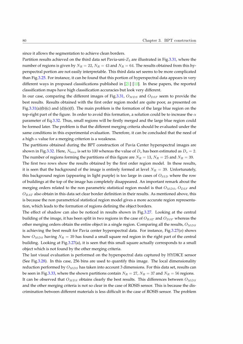
80 Chapter 3. BPT construction
since it allows the segmentation to achieve clean borders.
Partition results achieved on the third data set Pavia-uni-Z3 are illustrated in Fig.3.31, where the
number of regions is given by NR = 22, NR = 43 and NR = 64. The results obtained from this hy-
perspectral portion are not easily interpretable. This third data set seems to be more complicated
than Fig.3.25. For instance, it can be found that this portion of hyperspectral data appears in very
different ways in proposed classifications published in [21] [10]. In these papers, the reported
classification maps have high classification accuracies but look very different.
In our case, comparing the different images of Fig.3.31, OMDS and ODIF seem to provide the
best results. Results obtained with the first order region model are quite poor, as presented on
Fig.3.31(a)(b)(c) and (d)(e)(f). The main problem is the formation of the large blue region on the
top-right part of the figure. In order to avoid this formation, a solution could be to increase the ↵
parameter of Eq.3.32. Thus, small regions will be firstly merged and the large blue region could
be formed later. The problem is that the different merging criteria should be evaluated under the
same conditions in this experimental evaluation. Therefore, it can be concluded that the need of
a high ↵ value for a merging criterion is a weakness.
The partitions obtained during the BPT construction of Pavia Center hyperspectral images are
shown in Fig.3.32. Here, Nbins is set to 100 whereas the value of Ds has been estimated as Ds = 2.
The number of regions forming the partitions of this figure are NR = 13, NR = 25 and NR = 39.
The first two rows show the results obtained by the first order region model. In these results,
it is seen that the background of the image is entirely formed at level NR = 39. Unfortunately,
this background region (appearing in light purple) is too large in cases of OSID where the row
of buildings at the top of the image has completely disappeared. An important remark about the
merging orders related to the non parametric statistical region model is that OMDS , ODIF and
OBAT also obtain in this data set clear border definition in their results. As mentioned above, this
is because the non parametrical statistical region model gives a more accurate region representa-
tion, which leads to the formation of regions defining the object borders.
The effect of shadow can also be noticed in results shown in Fig.3.27. Looking at the central
building of the image, it has been split in two regions in the case of OBAT and ODIF whereas the
other merging orders obtain the entire object in a single region. Comparing all the results, OMDS
is achieving the best result for Pavia center hyperspectral data. For instance, Fig.3.27(o) shows
how OMDS having NR = 39 has found a small square red region in the right part of the central
building. Looking at Fig.3.27(a), it is seen that this small square actually corresponds to a small
object which is not found by the other merging criteria.
The last visual evaluation is performed on the hyperspectral data captured by HYDICE sensor
(See Fig.3.28). In this case, 256 bins are used to quantify this image. The local dimensionality
reduction performed by OMDS has taken into account 3 dimensions. For this data set, results can
be seen in Fig.3.33, where the shown partitions contain NR = 27, NR = 37 and NR = 56 regions.
It can be observed that OMDS obtains clearly the best results. This differences between OMDS
and the other merging criteria is not so clear in the case of ROSIS sensor. This is because the dis-
crimination between different materials is less difficult in the case of ROSIS sensor. The problem

3.4 Experimental Evaluation 81
is that there is a lower discrimination along all the spectral range in the Hydice image.
Also for this image, it can be seen that the merging orders OSID and OSAM have some problems.
For these two merging orders, buildings appear connected with roads. This can be observed at
the two first rows of Fig.3.33.
Comparing all the different results shown in Fig.3.29, Fig.3.30, Fig.3.31,Fig.3.32 and Fig.3.33, it is
not evident to perform an accurate classification of the merging orders according to their perfor-
mances. ODIF and OMDS seem to obtain the best results followed by OBC . However, in order to
evaluate more precisely the merging orders a quantitive evaluation should be done. This evalua-
tion is carried out in the following.
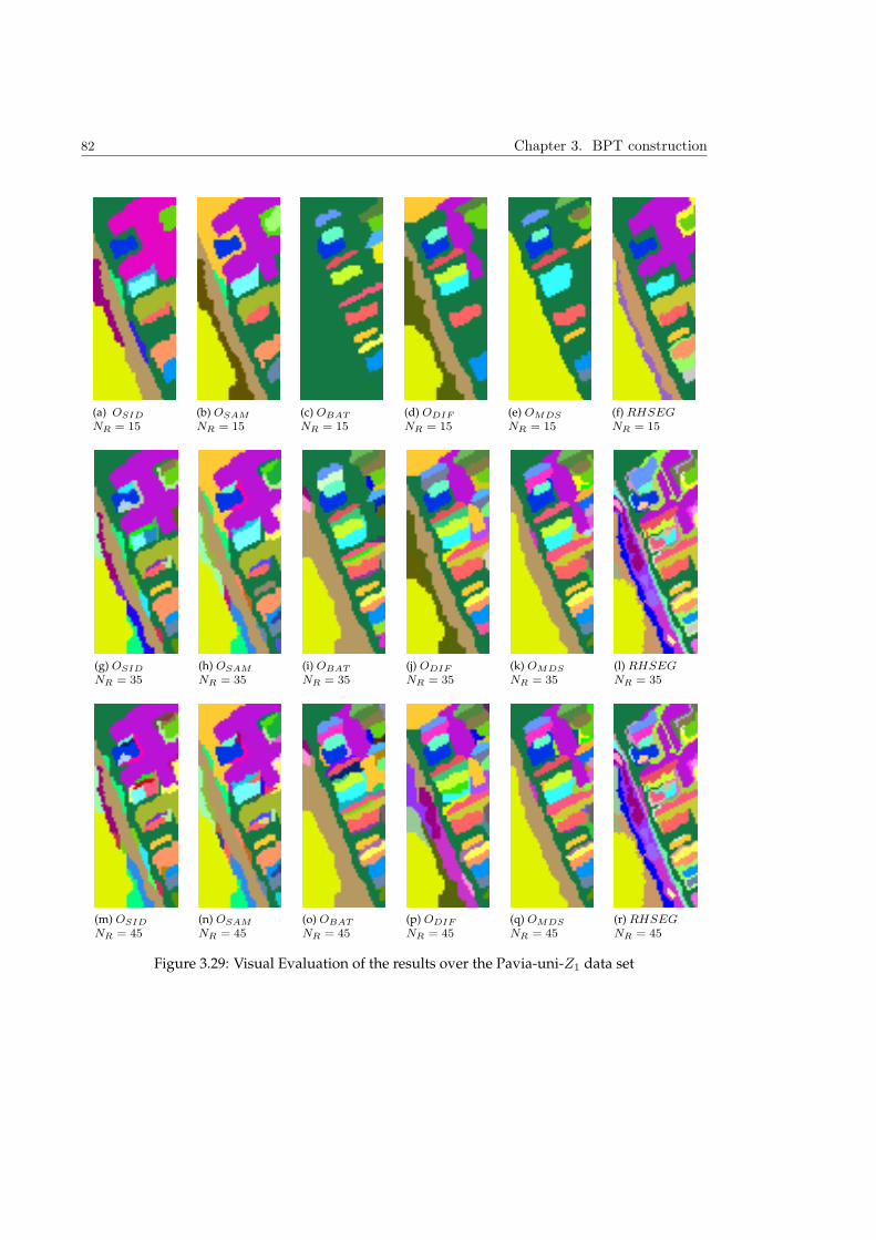
82 Chapter 3. BPT construction
(a) OSID
NR = 15(b) OSAM
NR = 15(c) OBAT
NR = 15(d) ODIF
NR = 15(e) OMDS
NR = 15(f) RHSEG
NR = 15
(g) OSID
NR = 35(h) OSAM
NR = 35(i) OBAT
NR = 35(j) ODIF
NR = 35(k) OMDS
NR = 35(l) RHSEG
NR = 35
(m) OSID
NR = 45(n) OSAM
NR = 45(o) OBAT
NR = 45(p) ODIF
NR = 45(q) OMDS
NR = 45(r) RHSEG
NR = 45
Figure 3.29: Visual Evaluation of the results over the Pavia-uni-Z1 data set
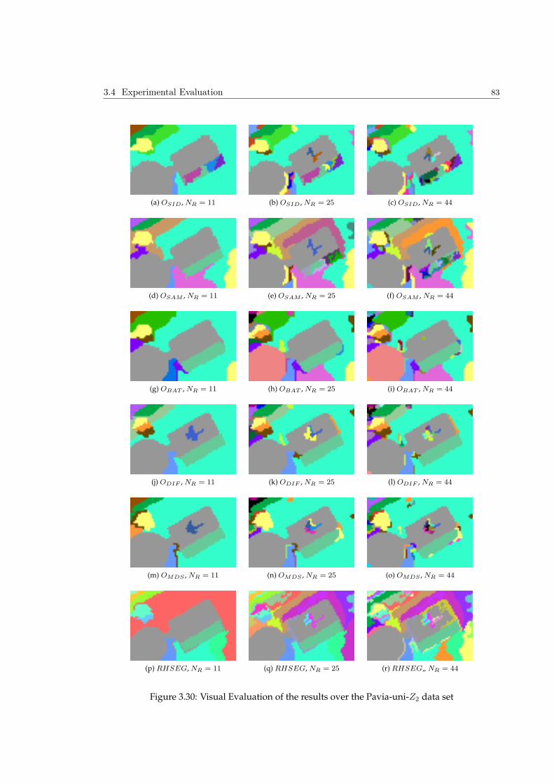
3.4 Experimental Evaluation 83
(a) OSID , NR = 11 (b) OSID , NR = 25 (c) OSID , NR = 44
(d) OSAM , NR = 11 (e) OSAM , NR = 25 (f) OSAM , NR = 44
(g) OBAT , NR = 11 (h) OBAT , NR = 25 (i) OBAT , NR = 44
(j) ODIF , NR = 11 (k) ODIF , NR = 25 (l) ODIF , NR = 44
(m) OMDS , NR = 11 (n) OMDS , NR = 25 (o) OMDS , NR = 44
(p) RHSEG, NR = 11 (q) RHSEG, NR = 25 (r) RHSEG„ NR = 44
Figure 3.30: Visual Evaluation of the results over the Pavia-uni-Z2 data set
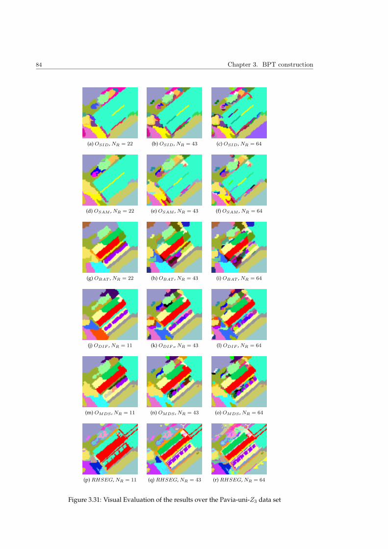
84 Chapter 3. BPT construction
(a) OSID , NR = 22 (b) OSID , NR = 43 (c) OSID , NR = 64
(d) OSAM , NR = 22 (e) OSAM , NR = 43 (f) OSAM , NR = 64
(g) OBAT , NR = 22 (h) OBAT , NR = 43 (i) OBAT , NR = 64
(j) ODIF , NR = 11 (k) ODIF „ NR = 43 (l) ODIF , NR = 64
(m) OMDS , NR = 11 (n) OMDS , NR = 43 (o) OMDS , NR = 64
(p) RHSEG, NR = 11 (q) RHSEG, NR = 43 (r) RHSEG, NR = 64
Figure 3.31: Visual Evaluation of the results over the Pavia-uni-Z3 data set
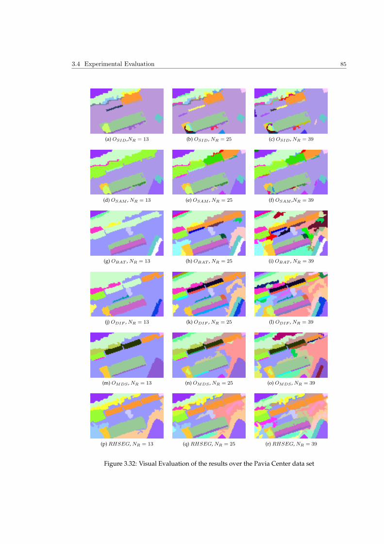
3.4 Experimental Evaluation 85
(a) OSID ,NR = 13 (b) OSID , NR = 25 (c) OSID , NR = 39
(d) OSAM , NR = 13 (e) OSAM , NR = 25 (f) OSAM ,NR = 39
(g) OBAT , NR = 13 (h) OBAT , NR = 25 (i) OBAT , NR = 39
(j) ODIF , NR = 13 (k) ODIF , NR = 25 (l) ODIF , NR = 39
(m) OMDS , NR = 13 (n) OMDS , NR = 25 (o) OMDS , NR = 39
(p) RHSEG, NR = 13 (q) RHSEG, NR = 25 (r) RHSEG, NR = 39
Figure 3.32: Visual Evaluation of the results over the Pavia Center data set
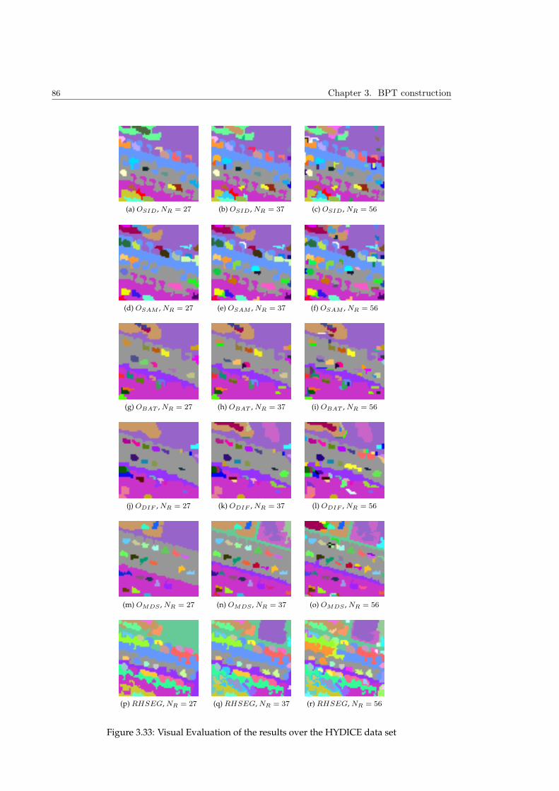
86 Chapter 3. BPT construction
(a) OSID , NR = 27 (b) OSID , NR = 37 (c) OSID , NR = 56
(d) OSAM , NR = 27 (e) OSAM , NR = 37 (f) OSAM , NR = 56
(g) OBAT , NR = 27 (h) OBAT , NR = 37 (i) OBAT , NR = 56
(j) ODIF , NR = 27 (k) ODIF , NR = 37 (l) ODIF , NR = 56
(m) OMDS , NR = 27 (n) OMDS , NR = 37 (o) OMDS , NR = 56
(p) RHSEG, NR = 27 (q) RHSEG, NR = 37 (r) RHSEG, NR = 56
Figure 3.33: Visual Evaluation of the results over the HYDICE data set
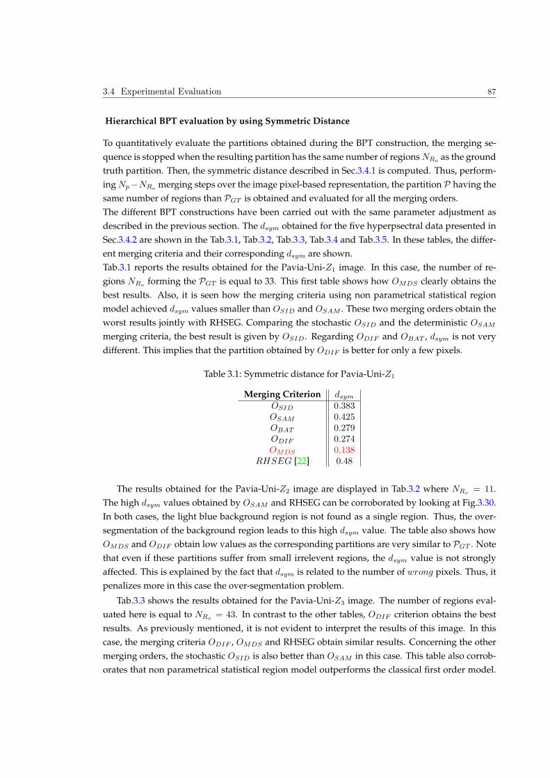
3.4 Experimental Evaluation 87
Hierarchical BPT evaluation by using Symmetric Distance
To quantitatively evaluate the partitions obtained during the BPT construction, the merging se-
quence is stopped when the resulting partition has the same number of regions NRoas the ground
truth partition. Then, the symmetric distance described in Sec.3.4.1 is computed. Thus, perform-
ing Np−NRomerging steps over the image pixel-based representation, the partition P having the
same number of regions than PGT is obtained and evaluated for all the merging orders.
The different BPT constructions have been carried out with the same parameter adjustment as
described in the previous section. The dsym obtained for the five hyperpsectral data presented in
Sec.3.4.2 are shown in the Tab.3.1, Tab.3.2, Tab.3.3, Tab.3.4 and Tab.3.5. In these tables, the differ-
ent merging criteria and their corresponding dsym are shown.
Tab.3.1 reports the results obtained for the Pavia-Uni-Z1 image. In this case, the number of re-
gions NRoforming the PGT is equal to 33. This first table shows how OMDS clearly obtains the
best results. Also, it is seen how the merging criteria using non parametrical statistical region
model achieved dsym values smaller than OSID and OSAM . These two merging orders obtain the
worst results jointly with RHSEG. Comparing the stochastic OSID and the deterministic OSAM
merging criteria, the best result is given by OSID. Regarding ODIF and OBAT , dsym is not very
different. This implies that the partition obtained by ODIF is better for only a few pixels.
Table 3.1: Symmetric distance for Pavia-Uni-Z1
Merging Criterion dsymOSID 0.383OSAM 0.425OBAT 0.279ODIF 0.274OMDS 0.138
RHSEG [22] 0.48
The results obtained for the Pavia-Uni-Z2 image are displayed in Tab.3.2 where NRo= 11.
The high dsym values obtained by OSAM and RHSEG can be corroborated by looking at Fig.3.30.
In both cases, the light blue background region is not found as a single region. Thus, the over-
segmentation of the background region leads to this high dsym value. The table also shows how
OMDS and ODIF obtain low values as the corresponding partitions are very similar to PGT . Note
that even if these partitions suffer from small irrelevent regions, the dsym value is not strongly
affected. This is explained by the fact that dsym is related to the number of wrong pixels. Thus, it
penalizes more in this case the over-segmentation problem.
Tab.3.3 shows the results obtained for the Pavia-Uni-Z3 image. The number of regions eval-
uated here is equal to NRo= 43. In contrast to the other tables, ODIF criterion obtains the best
results. As previously mentioned, it is not evident to interpret the results of this image. In this
case, the merging criteria ODIF , OMDS and RHSEG obtain similar results. Concerning the other
merging orders, the stochastic OSID is also better than OSAM in this case. This table also corrob-
orates that non parametrical statistical region model outperforms the classical first order model.

88 Chapter 3. BPT construction
Table 3.2: Symmetric distance for Pavia-Uni-Z2
Merging Criterion dsymOSID 0.175OSAM 0.303OBAT 0.186ODIF 0.132OMDS 0.108
RHSEG [22] 0.202
The robustness of ODIF to Nbins lead to better results as compared to the OBAT criterion.
Table 3.3: Symmetric distance for Pavia-uni-Z3
Merging Criterion dsymOSID 0.427OSAM 0.434OBAT 0.303ODIF 0.239OMDS 0.269
RHSEG [22] 0.272
Results obtained for the Pavia Center image are presented in Tab.3.4. The number of regions
contained in PGT are in this case equal to 23. As in the first two tables, OMDS achieves also here
the best result. However, the second best result is achieved by OSAM in this case. It is observed
how the partition of Fig.3.32 (e) is close to the PGT of Fig.3.27(b). For this example, one of the main
problems of OBAT and ODIF is the division of the central building of the image. Concerning the
background region, the over-segmentation error is also important in OMDS , OBAT , ODIF and
RHSEG. Thus, these merging orders increase their dsym value.
Table 3.4: Symmetric distance for Pavia Center
Merging Criterion dsymOSID 0.336OSAM 0.225OBAT 0.286ODIF 0.274OMDS 0.227
RHSEG [22] 0.48
Finally, the dsym evaluation by Hydice image is reported in Tab.3.5. The obtained results
evaluate partitions containing 56 regions with the PGT partition shown in Fig.3.28(b). The table
corroborates the visual results illustrated on Fig.3.33.
OMDS is also here the best merging criterion which can also be seen in Fig.3.33(m)(n)(o). For this
criterion, the different zones of the images as building, roads and background are correctly sep-
arated. As in the previous data sets, merging orders which rely on the non-parametric statistical
region model obviously outperforms the OSID and OSAM criteria. Comparing ODIF and OBAT ,
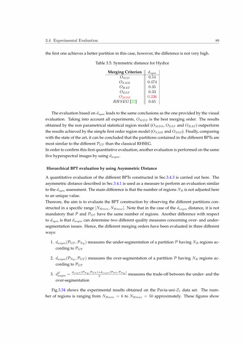
3.4 Experimental Evaluation 89
the first one achieves a better partition in this case, however, the difference is not very high.
Table 3.5: Symmetric distance for Hydice
Merging Criterion dsymOSID 0.54OSAM 0.474OBAT 0.35ODIF 0.33OMDS 0.236
RHSEG [22] 0.65
The evaluation based on dsym leads to the same conclusions as the one provided by the visual
evaluation. Taking into account all experiments, OMDS is the best merging order. The results
obtained by the non parametrical statistical region model (OMDS , ODIF and OBAT ) outperform
the results achieved by the simple first order region model (OSAM and OSID). Finally, comparing
with the state of the art, it can be concluded that the partitions contained in the different BPTs are
most similar to the different PGT than the classical RHSEG.
In order to confirm this first quantitative evaluation, another evaluation is performed on the same
five hyperspectral images by using dasym.
Hierarchical BPT evaluation by using Asymmetric Distance
A quantitative evaluation of the different BPTs constructed in Sec.3.4.3 is carried out here. The
asymmetric distance described in Sec.3.4.1 is used as a measure to perform an evaluation similar
to the dsym assessment. The main difference is that the number of regions NR is not adjusted here
to an unique value.
Thereore, the aim is to evaluate the BPT construction by observing the different partitions con-
structed in a specific range [NRmin, NRmax]. Note that in the case of the dasym distance, it is not
mandatory that P and PGT have the same number of regions. Another difference with respect
to dsym is that dasym can determine two different quality measures concerning over- and under-
segmentation issues. Hence, the different merging orders have been evaluated in three different
ways:
1. dasym(PGT ,PNR) measures the under-segmentation of a partition P having NR regions ac-
cording to PGT
2. dasym(PNR,PGT ) measures the over-segmentation of a partition P having NR regions ac-
cording to PGT
3. dTasym =dasym(PNR
,PGT )+dasym(PGT ,PNR)
2 measures the trade-off between the under- and the
over-segmentation
Fig.3.34 shows the experimental results obtained on the Pavia-uni-Z1 data set. The num-
ber of regions is ranging from NRmin = 6 to NRmax = 50 approximately. These figures show
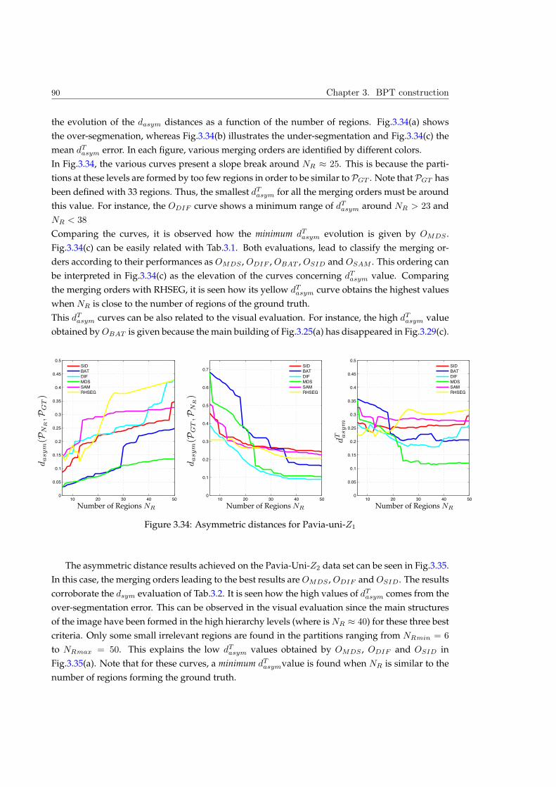
90 Chapter 3. BPT construction
the evolution of the dasym distances as a function of the number of regions. Fig.3.34(a) shows
the over-segmenation, whereas Fig.3.34(b) illustrates the under-segmentation and Fig.3.34(c) the
mean dTasym error. In each figure, various merging orders are identified by different colors.
In Fig.3.34, the various curves present a slope break around NR 25. This is because the parti-
tions at these levels are formed by too few regions in order to be similar to PGT . Note that PGT has
been defined with 33 regions. Thus, the smallest dTasym for all the merging orders must be around
this value. For instance, the ODIF curve shows a minimum range of dTasym around NR > 23 and
NR < 38
Comparing the curves, it is observed how the minimum dTasym evolution is given by OMDS .
Fig.3.34(c) can be easily related with Tab.3.1. Both evaluations, lead to classify the merging or-
ders according to their performances as OMDS , ODIF , OBAT , OSID and OSAM . This ordering can
be interpreted in Fig.3.34(c) as the elevation of the curves concerning dTasym value. Comparing
the merging orders with RHSEG, it is seen how its yellow dTasym curve obtains the highest values
when NR is close to the number of regions of the ground truth.
This dTasym curves can be also related to the visual evaluation. For instance, the high dTasym value
obtained by OBAT is given because the main building of Fig.3.25(a) has disappeared in Fig.3.29(c).
10 20 30 40 500
0.05
0.1
0.15
0.2
0.25
0.3
0.35
0.4
0.45
0.5
SID
BAT
DIF
MDS
SAM
RHSEG
10 20 30 40 500
0.1
0.2
0.3
0.4
0.5
0.6
0.7
SID
BAT
DIF
MDS
SAM
RHSEG
10 20 30 40 500
0.05
0.1
0.15
0.2
0.25
0.3
0.35
0.4
0.45
0.5
SID
BAT
DIF
MDS
SAM
RHSEG
dasym(P
NR,P
GT)
dasym(P
GT,P
NR)
dT asym
Number of Regions NRNumber of Regions NRNumber of Regions NR
Figure 3.34: Asymmetric distances for Pavia-uni-Z1
The asymmetric distance results achieved on the Pavia-Uni-Z2 data set can be seen in Fig.3.35.
In this case, the merging orders leading to the best results are OMDS , ODIF and OSID. The results
corroborate the dsym evaluation of Tab.3.2. It is seen how the high values of dTasym comes from the
over-segmentation error. This can be observed in the visual evaluation since the main structures
of the image have been formed in the high hierarchy levels (where is NR 40) for these three best
criteria. Only some small irrelevant regions are found in the partitions ranging from NRmin = 6
to NRmax = 50. This explains the low dTasym values obtained by OMDS , ODIF and OSID in
Fig.3.35(a). Note that for these curves, a minimum dTasymvalue is found when NR is similar to the
number of regions forming the ground truth.
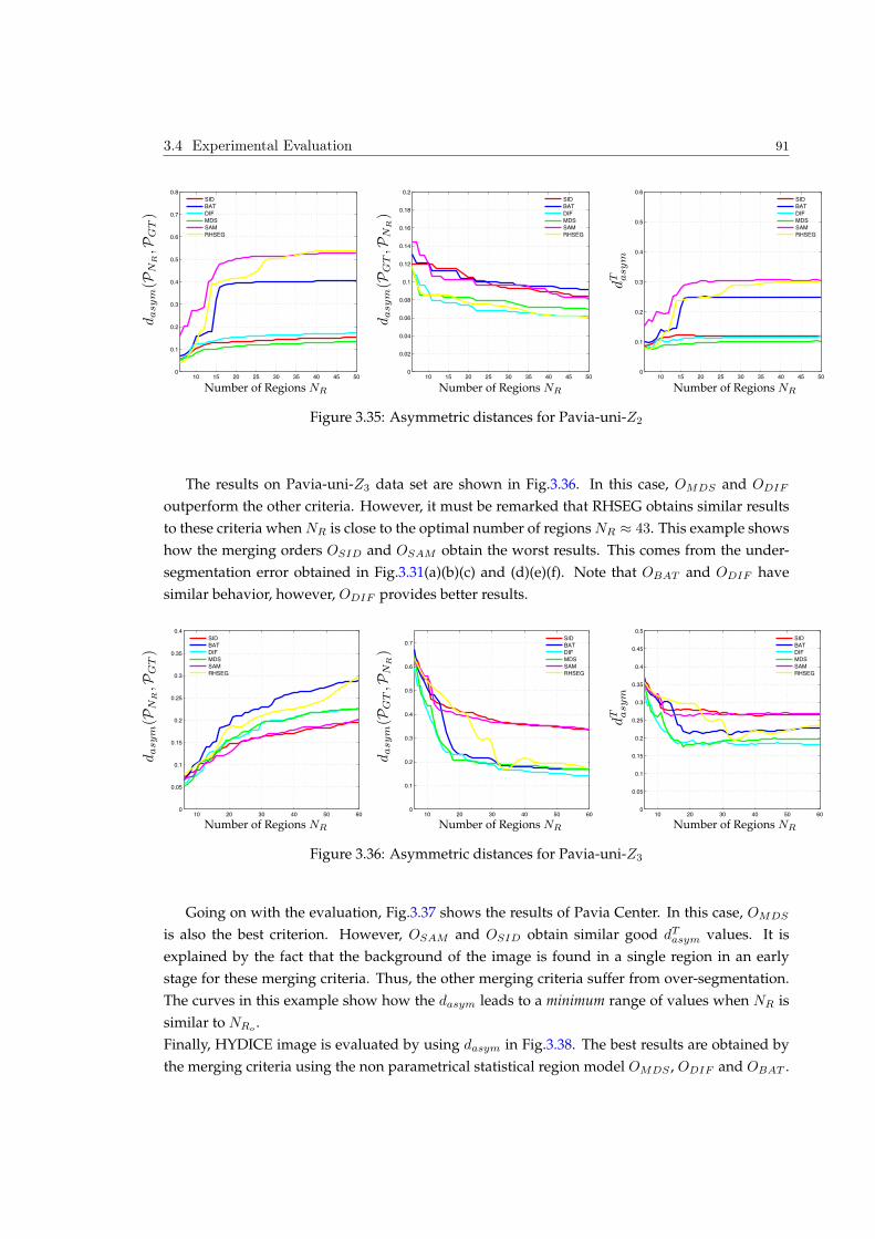
3.4 Experimental Evaluation 91
10 15 20 25 30 35 40 45 500
0.1
0.2
0.3
0.4
0.5
0.6
0.7
0.8
SID
BAT
DIF
MDS
SAM
RHSEG
10 15 20 25 30 35 40 45 500
0.02
0.04
0.06
0.08
0.1
0.12
0.14
0.16
0.18
0.2
SID
BAT
DIF
MDS
SAM
RHSEG
10 15 20 25 30 35 40 45 500
0.1
0.2
0.3
0.4
0.5
0.6
SID
BAT
DIF
MDS
SAM
RHSEG
dasym(P
NR,P
GT)
dasym(P
GT,P
NR)
dT asym
Number of Regions NRNumber of Regions NRNumber of Regions NR
Figure 3.35: Asymmetric distances for Pavia-uni-Z2
The results on Pavia-uni-Z3 data set are shown in Fig.3.36. In this case, OMDS and ODIF
outperform the other criteria. However, it must be remarked that RHSEG obtains similar results
to these criteria when NR is close to the optimal number of regions NR 43. This example shows
how the merging orders OSID and OSAM obtain the worst results. This comes from the under-
segmentation error obtained in Fig.3.31(a)(b)(c) and (d)(e)(f). Note that OBAT and ODIF have
similar behavior, however, ODIF provides better results.
10 20 30 40 50 600
0.05
0.1
0.15
0.2
0.25
0.3
0.35
0.4
SID
BAT
DIF
MDS
SAM
RHSEG
10 20 30 40 50 600
0.1
0.2
0.3
0.4
0.5
0.6
0.7
SID
BAT
DIF
MDS
SAM
RHSEG
10 20 30 40 50 600
0.05
0.1
0.15
0.2
0.25
0.3
0.35
0.4
0.45
0.5
SID
BAT
DIF
MDS
SAM
RHSEG
dasym(P
NR,P
GT)
dasym(P
GT,P
NR)
dT asym
Number of Regions NRNumber of Regions NRNumber of Regions NR
Figure 3.36: Asymmetric distances for Pavia-uni-Z3
Going on with the evaluation, Fig.3.37 shows the results of Pavia Center. In this case, OMDS
is also the best criterion. However, OSAM and OSID obtain similar good dTasym values. It is
explained by the fact that the background of the image is found in a single region in an early
stage for these merging criteria. Thus, the other merging criteria suffer from over-segmentation.
The curves in this example show how the dasym leads to a minimum range of values when NR is
similar to NRo.
Finally, HYDICE image is evaluated by using dasym in Fig.3.38. The best results are obtained by
the merging criteria using the non parametrical statistical region model OMDS , ODIF and OBAT .
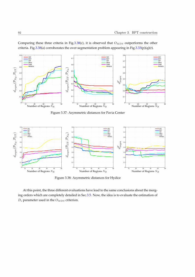
92 Chapter 3. BPT construction
Comparing these three criteria in Fig.3.38(c), it is observed that OMDS outperforms the other
criteria. Fig.3.38(a) corroborates the over-segmentation problem appearing in Fig.3.33(p)(q)(r).
10 20 30 40 500
0.1
0.2
0.3
0.4
0.5
0.6
0.7
0.8
SID
BAT
DIF
MDS
SAM
RHSEG
10 20 30 40 500
0.1
0.2
0.3
0.4
0.5
0.6
0.7
SID
BAT
DIF
MDS
SAM
RHSEG
10 20 30 40 500
0.1
0.2
0.3
0.4
0.5
0.6
0.7
0.8
SID
BAT
DIF
MDS
SAM
RHSEG
dasym(P
NR,P
GT)
dasym(P
GT,P
NR)
dT asym
Number of Regions NRNumber of Regions NRNumber of Regions NR
Figure 3.37: Asymmetric distances for Pavia Center
10 20 30 40 50 600
0.1
0.2
0.3
0.4
0.5
0.6
0.7
0.8
SID
BAT
DIF
MDS
SAM
RHSEG
10 20 30 40 50 600
0.1
0.2
0.3
0.4
0.5
0.6
0.7
0.8
SID
BAT
DIF
MDS
SAM
RHSEG
10 20 30 40 50 600
0.1
0.2
0.3
0.4
0.5
0.6
0.7
0.8
SID
BAT
DIF
MDS
SAM
RHSEG
dasym(P
NR,P
GT)
dasym(P
GT,P
NR)
dT asym
Number of Regions NRNumber of Regions NRNumber of Regions NR
Figure 3.38: Asymmetric distances for Hydice
At this point, the three different evaluations have lead to the same conclusions about the merg-
ing orders which are completely detailed in Sec.3.5. Now, the idea is to evaluate the estimation of
Ds parameter used in the OMDS criterion.
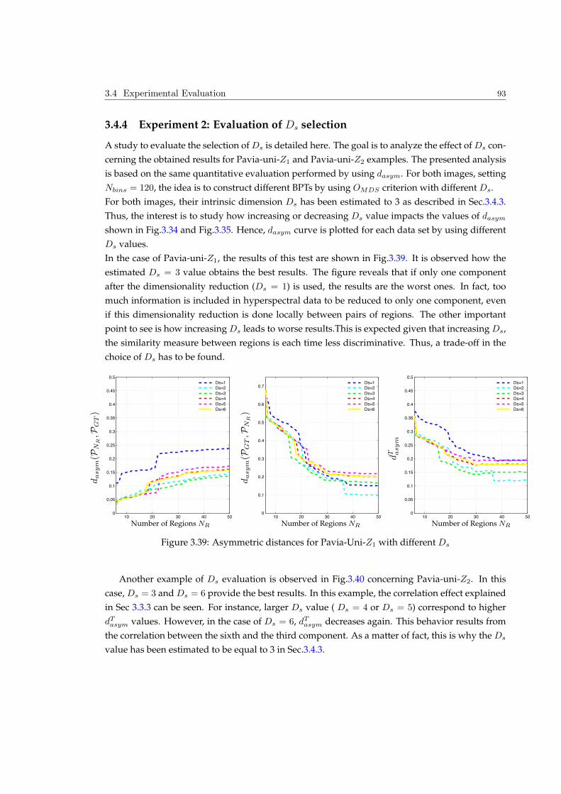
3.4 Experimental Evaluation 93
3.4.4 Experiment 2: Evaluation of Ds selection
A study to evaluate the selection of Ds is detailed here. The goal is to analyze the effect of Ds con-
cerning the obtained results for Pavia-uni-Z1 and Pavia-uni-Z2 examples. The presented analysis
is based on the same quantitative evaluation performed by using dasym. For both images, setting
Nbins = 120, the idea is to construct different BPTs by using OMDS criterion with different Ds.
For both images, their intrinsic dimension Ds has been estimated to 3 as described in Sec.3.4.3.
Thus, the interest is to study how increasing or decreasing Ds value impacts the values of dasym
shown in Fig.3.34 and Fig.3.35. Hence, dasym curve is plotted for each data set by using different
Ds values.
In the case of Pavia-uni-Z1, the results of this test are shown in Fig.3.39. It is observed how the
estimated Ds = 3 value obtains the best results. The figure reveals that if only one component
after the dimensionality reduction (Ds = 1) is used, the results are the worst ones. In fact, too
much information is included in hyperspectral data to be reduced to only one component, even
if this dimensionality reduction is done locally between pairs of regions. The other important
point to see is how increasing Ds leads to worse results.This is expected given that increasing Ds,
the similarity measure between regions is each time less discriminative. Thus, a trade-off in the
choice of Ds has to be found.
10 20 30 40 500
0.05
0.1
0.15
0.2
0.25
0.3
0.35
0.4
0.45
0.5
Ds=1
Ds=2
Ds=3
Ds=4
Ds=5
Ds=6
10 20 30 40 500
0.1
0.2
0.3
0.4
0.5
0.6
0.7
Ds=1
Ds=2
Ds=3
Ds=4
Ds=5
Ds=6
10 20 30 40 500
0.05
0.1
0.15
0.2
0.25
0.3
0.35
0.4
0.45
0.5
Ds=1
Ds=2
Ds=3
Ds=4
Ds=5
Ds=6
dasym(P
NR,P
GT)
dasym(P
GT,P
NR)
dT asym
Number of Regions NRNumber of Regions NRNumber of Regions NR
Figure 3.39: Asymmetric distances for Pavia-Uni-Z1 with different Ds
Another example of Ds evaluation is observed in Fig.3.40 concerning Pavia-uni-Z2. In this
case, Ds = 3 and Ds = 6 provide the best results. In this example, the correlation effect explained
in Sec 3.3.3 can be seen. For instance, larger Ds value ( Ds = 4 or Ds = 5) correspond to higher
dTasym values. However, in the case of Ds = 6, dTasym decreases again. This behavior results from
the correlation between the sixth and the third component. As a matter of fact, this is why the Ds
value has been estimated to be equal to 3 in Sec.3.4.3.
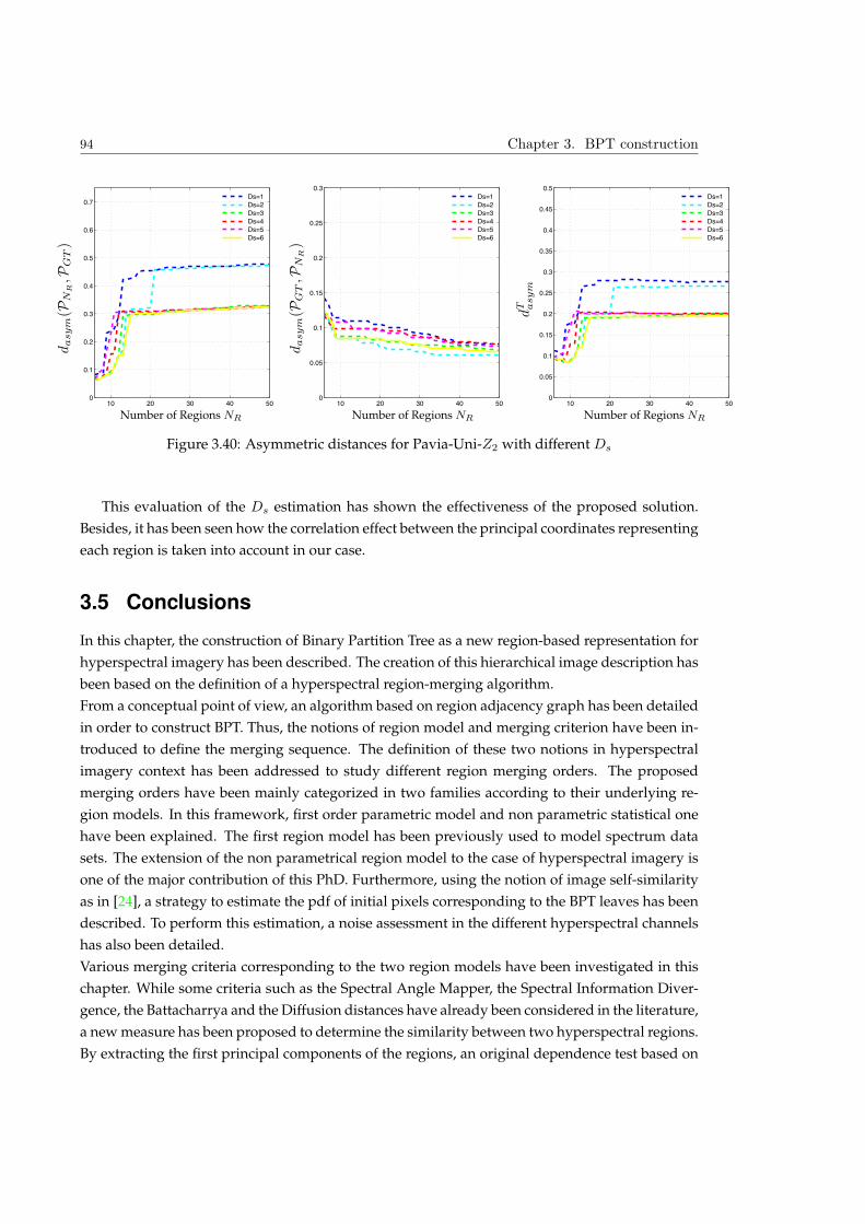
94 Chapter 3. BPT construction
10 20 30 40 500
0.1
0.2
0.3
0.4
0.5
0.6
0.7
Ds=1
Ds=2
Ds=3
Ds=4
Ds=5
Ds=6
10 20 30 40 500
0.05
0.1
0.15
0.2
0.25
0.3
Ds=1
Ds=2
Ds=3
Ds=4
Ds=5
Ds=6
10 20 30 40 500
0.05
0.1
0.15
0.2
0.25
0.3
0.35
0.4
0.45
0.5
Ds=1
Ds=2
Ds=3
Ds=4
Ds=5
Ds=6
dasym(P
NR,P
GT)
dasym(P
GT,P
NR)
dT asym
Number of Regions NRNumber of Regions NRNumber of Regions NR
Figure 3.40: Asymmetric distances for Pavia-Uni-Z2 with different Ds
This evaluation of the Ds estimation has shown the effectiveness of the proposed solution.
Besides, it has been seen how the correlation effect between the principal coordinates representing
each region is taken into account in our case.
3.5 Conclusions
In this chapter, the construction of Binary Partition Tree as a new region-based representation for
hyperspectral imagery has been described. The creation of this hierarchical image description has
been based on the definition of a hyperspectral region-merging algorithm.
From a conceptual point of view, an algorithm based on region adjacency graph has been detailed
in order to construct BPT. Thus, the notions of region model and merging criterion have been in-
troduced to define the merging sequence. The definition of these two notions in hyperspectral
imagery context has been addressed to study different region merging orders. The proposed
merging orders have been mainly categorized in two families according to their underlying re-
gion models. In this framework, first order parametric model and non parametric statistical one
have been explained. The first region model has been previously used to model spectrum data
sets. The extension of the non parametrical region model to the case of hyperspectral imagery is
one of the major contribution of this PhD. Furthermore, using the notion of image self-similarity
as in [24], a strategy to estimate the pdf of initial pixels corresponding to the BPT leaves has been
described. To perform this estimation, a noise assessment in the different hyperspectral channels
has also been detailed.
Various merging criteria corresponding to the two region models have been investigated in this
chapter. While some criteria such as the Spectral Angle Mapper, the Spectral Information Diver-
gence, the Battacharrya and the Diffusion distances have already been considered in the literature,
a new measure has been proposed to determine the similarity between two hyperspectral regions.
By extracting the first principal components of the regions, an original dependence test based on
3.5 Conclusions 95
MANOVA theory has been proposed to measure the correlation between two spectrum data sets.
To our knowledge, the MDS dimensionality reduction technique proposed here introduces a nov-
elty regarding the state of the art and is another contribution of our work. In the literature, au-
thors have focused on the reduction of the dimensionality of hyperspectral data by studying the
global image statistics. Contrarily, this Phd has proposed to extract local principal components
by studying the local statistics of the regions. This local dimensionality reduction has lead to a
more accurate representation of the regions.
Furthermore, a new method to extract the intrinsic dimensionality of the hyperspectral regions
has also been described. The idea of correlation between the extracted principal components have
been presented here.
A sensitivity study has been carried out to determine the performances of the proposed merging
orders. The construction of different BPTs using the different region models and merging criteria
has been investigated. Five different hyperspectral images have been selected for this study. Be-
sides comparing the different merging orders, the partitions obtained by BPT are also compared
with the state-of-the-art.
The analysis of the partitions contained in the BPT hierarchical levels has been addressed by
three different evaluations. Firstly, a visual assessment of the partitions formed during the merg-
ing construction has been analyzed. Secondly, a quantitative evaluation by using different quality
measures (dsym and dasym) has been performed. These measures have led to determine over-and
under-segmentations errors committed during the BPT construction.
The results obtained by the three different evaluations lead to the same conclusions. The non-
parametric statistical model clearly outperforms the simple first-order model. Given the com-
plexity of the scene, the first-order model has shown its limitation in order to represent spectrum
data sets. Contrarily, non parametrical statistical region model has shown its effectiveness in
order to model the spectral variability. In particular, the obtained results have shown a high ac-
curacy and robustness with respect to borders.
Comparing the stochastic and deterministic merging criteria used with first-order region model,
SID has obtained better result than SAM.
An evaluation between the different merging criteria proposed to be used with the non para-
metric statistical region model has also been done. For the three presented similarity measures,
Battacharyya distance obtains the worst results which is explained by its lack of robustness in
case of histogram misalignment. Thus, an improvement on the results has been introduced by
the cross-bin Diffusion distance. Note that this distance gives more precise information taking
into account cross-bin contributions. However, the problem of Battacharrya and Diffusion dis-
tance is that the spectral information is not jointly studied. Thus, the correlation of the channels
and the importance of the relevant information is not taken into account by these merging criteria.
Contrarily, the similarity measure proposed via multidimensionality scaling metric has dealt with
all these problems. For this reason, the merging order interpreted as the canonical correlation has
achieved the best results. In all the cases, the merging criterion based on MDS and the MANOVA
dependence test has constructed the best BPT image representation.

96 Chapter 3. BPT construction
Besides the experiments aiming at the evaluation of the partitions obtained during the BPT con-
struction, another experiment has shown the importance of the Ds choice. The number of dimen-
sions used to measure the similarity between hyperspectral regions is an important parameter
and an algorithm estimating its value has been proposed.

4BPT Pruning Strategies
Contents
4.1 Introduction . . . . . . . . . . . . . . . . . . . . . . . . . . . . . . . . . . . . . . . . 98
4.2 Supervised Hyperspectral Classification . . . . . . . . . . . . . . . . . . . . . . . 103
4.2.1 Populating the BPT . . . . . . . . . . . . . . . . . . . . . . . . . . . . . . . . 103
4.2.2 Pruning Decision . . . . . . . . . . . . . . . . . . . . . . . . . . . . . . . . . 105
4.2.3 Experimental results . . . . . . . . . . . . . . . . . . . . . . . . . . . . . . . 107
4.3 Segmentation by Energy Minimization Strategy . . . . . . . . . . . . . . . . . . . 115
4.3.1 The D(N ) definition . . . . . . . . . . . . . . . . . . . . . . . . . . . . . . . 118
4.3.2 Homogeneity measure . . . . . . . . . . . . . . . . . . . . . . . . . . . . . . 118
4.3.3 Experimental Results . . . . . . . . . . . . . . . . . . . . . . . . . . . . . . . 119
4.4 Segmentation by recursive spectral graph partitioning . . . . . . . . . . . . . . . 124
4.4.1 The BPT node weight WN . . . . . . . . . . . . . . . . . . . . . . . . . . . . 124
4.4.2 Local Branch partitioning . . . . . . . . . . . . . . . . . . . . . . . . . . . . . 126
4.4.3 Experimental Results . . . . . . . . . . . . . . . . . . . . . . . . . . . . . . . 130
4.5 Object detection . . . . . . . . . . . . . . . . . . . . . . . . . . . . . . . . . . . . . . 135
4.5.1 Detection of roads . . . . . . . . . . . . . . . . . . . . . . . . . . . . . . . . . 136
4.5.2 Detection of buildings . . . . . . . . . . . . . . . . . . . . . . . . . . . . . . 137
4.5.3 Experimental Results . . . . . . . . . . . . . . . . . . . . . . . . . . . . . . . 138
4.6 Conclusions . . . . . . . . . . . . . . . . . . . . . . . . . . . . . . . . . . . . . . . . 140
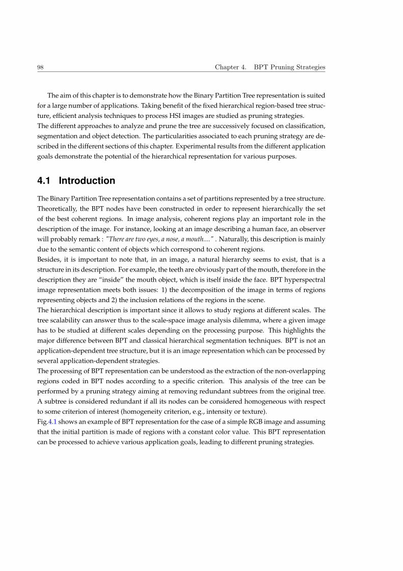
98 Chapter 4. BPT Pruning Strategies
The aim of this chapter is to demonstrate how the Binary Partition Tree representation is suited
for a large number of applications. Taking benefit of the fixed hierarchical region-based tree struc-
ture, efficient analysis techniques to process HSI images are studied as pruning strategies.
The different approaches to analyze and prune the tree are successively focused on classification,
segmentation and object detection. The particularities associated to each pruning strategy are de-
scribed in the different sections of this chapter. Experimental results from the different application
goals demonstrate the potential of the hierarchical representation for various purposes.
4.1 Introduction
The Binary Partition Tree representation contains a set of partitions represented by a tree structure.
Theoretically, the BPT nodes have been constructed in order to represent hierarchically the set
of the best coherent regions. In image analysis, coherent regions play an important role in the
description of the image. For instance, looking at an image describing a human face, an observer
will probably remark : "There are two eyes, a nose, a mouth...." . Naturally, this description is mainly
due to the semantic content of objects which correspond to coherent regions.
Besides, it is important to note that, in an image, a natural hierarchy seems to exist, that is a
structure in its description. For example, the teeth are obviously part of the mouth, therefore in the
description they are “inside” the mouth object, which is itself inside the face. BPT hyperspectral
image representation meets both issues: 1) the decomposition of the image in terms of regions
representing objects and 2) the inclusion relations of the regions in the scene.
The hierarchical description is important since it allows to study regions at different scales. The
tree scalability can answer thus to the scale-space image analysis dilemma, where a given image
has to be studied at different scales depending on the processing purpose. This highlights the
major difference between BPT and classical hierarchical segmentation techniques. BPT is not an
application-dependent tree structure, but it is an image representation which can be processed by
several application-dependent strategies.
The processing of BPT representation can be understood as the extraction of the non-overlapping
regions coded in BPT nodes according to a specific criterion. This analysis of the tree can be
performed by a pruning strategy aiming at removing redundant subtrees from the original tree.
A subtree is considered redundant if all its nodes can be considered homogeneous with respect
to some criterion of interest (homogeneity criterion, e.g., intensity or texture).
Fig.4.1 shows an example of BPT representation for the case of a simple RGB image and assuming
that the initial partition is made of regions with a constant color value. This BPT representation
can be processed to achieve various application goals, leading to different pruning strategies.
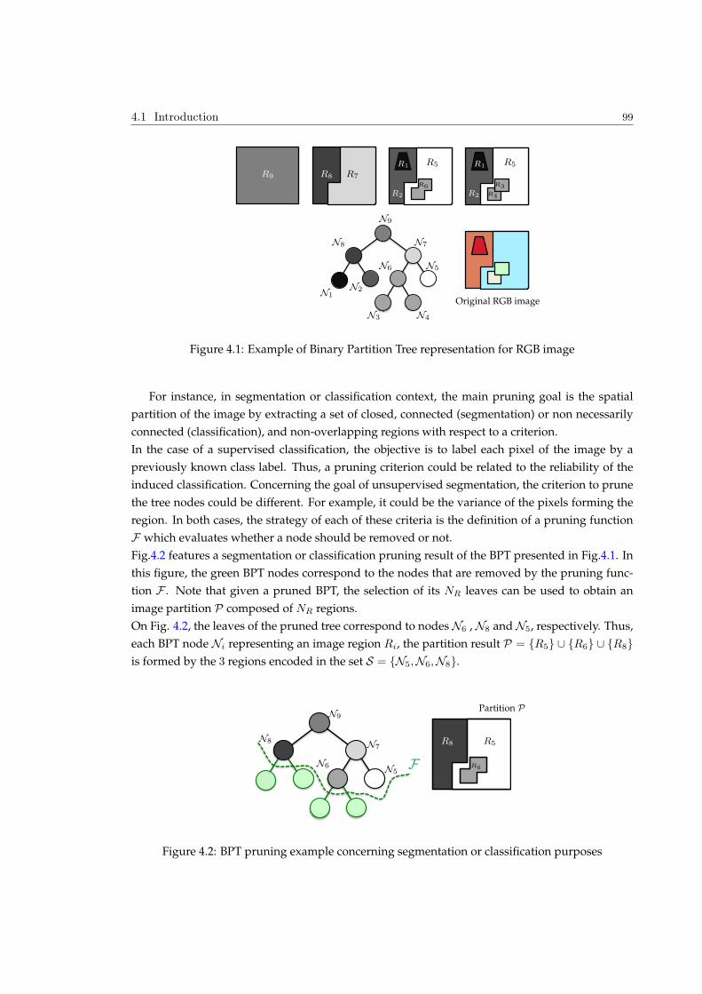
4.1 Introduction 99
N1
N2
R1
R2
R1
R2
N3 N4
R3
R4
N6
R6
N5
Original RGB image
R5 R5
N7N8
N9
R7R8R9
Figure 4.1: Example of Binary Partition Tree representation for RGB image
For instance, in segmentation or classification context, the main pruning goal is the spatial
partition of the image by extracting a set of closed, connected (segmentation) or non necessarily
connected (classification), and non-overlapping regions with respect to a criterion.
In the case of a supervised classification, the objective is to label each pixel of the image by a
previously known class label. Thus, a pruning criterion could be related to the reliability of the
induced classification. Concerning the goal of unsupervised segmentation, the criterion to prune
the tree nodes could be different. For example, it could be the variance of the pixels forming the
region. In both cases, the strategy of each of these criteria is the definition of a pruning function
F which evaluates whether a node should be removed or not.
Fig.4.2 features a segmentation or classification pruning result of the BPT presented in Fig.4.1. In
this figure, the green BPT nodes correspond to the nodes that are removed by the pruning func-
tion F . Note that given a pruned BPT, the selection of its NR leaves can be used to obtain an
image partition P composed of NR regions.
On Fig. 4.2, the leaves of the pruned tree correspond to nodes N6 , N8 and N5, respectively. Thus,
each BPT node Ni representing an image region Ri, the partition result P = R5 [ R6 [ R8
is formed by the 3 regions encoded in the set S = N5,N6,N8.
N6N5
F
N7
N8
N9
R5
Partition P
R6
R8
Figure 4.2: BPT pruning example concerning segmentation or classification purposes
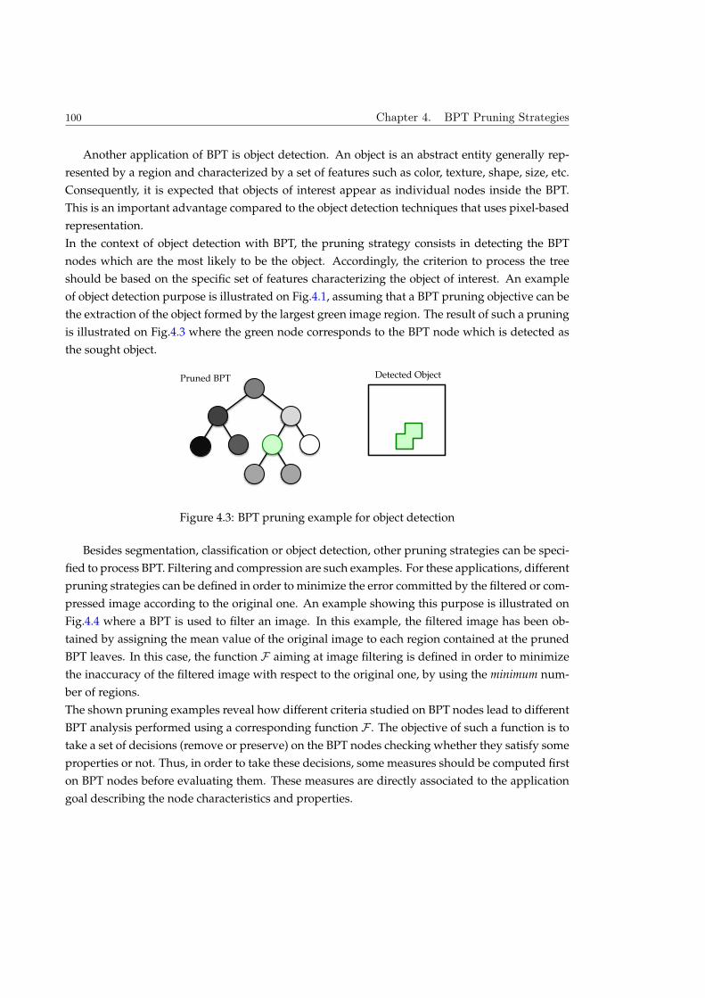
100 Chapter 4. BPT Pruning Strategies
Another application of BPT is object detection. An object is an abstract entity generally rep-
resented by a region and characterized by a set of features such as color, texture, shape, size, etc.
Consequently, it is expected that objects of interest appear as individual nodes inside the BPT.
This is an important advantage compared to the object detection techniques that uses pixel-based
representation.
In the context of object detection with BPT, the pruning strategy consists in detecting the BPT
nodes which are the most likely to be the object. Accordingly, the criterion to process the tree
should be based on the specific set of features characterizing the object of interest. An example
of object detection purpose is illustrated on Fig.4.1, assuming that a BPT pruning objective can be
the extraction of the object formed by the largest green image region. The result of such a pruning
is illustrated on Fig.4.3 where the green node corresponds to the BPT node which is detected as
the sought object.
Pruned BPT Detected Object
Figure 4.3: BPT pruning example for object detection
Besides segmentation, classification or object detection, other pruning strategies can be speci-
fied to process BPT. Filtering and compression are such examples. For these applications, different
pruning strategies can be defined in order to minimize the error committed by the filtered or com-
pressed image according to the original one. An example showing this purpose is illustrated on
Fig.4.4 where a BPT is used to filter an image. In this example, the filtered image has been ob-
tained by assigning the mean value of the original image to each region contained at the pruned
BPT leaves. In this case, the function F aiming at image filtering is defined in order to minimize
the inaccuracy of the filtered image with respect to the original one, by using the minimum num-
ber of regions.
The shown pruning examples reveal how different criteria studied on BPT nodes lead to different
BPT analysis performed using a corresponding function F . The objective of such a function is to
take a set of decisions (remove or preserve) on the BPT nodes checking whether they satisfy some
properties or not. Thus, in order to take these decisions, some measures should be computed first
on BPT nodes before evaluating them. These measures are directly associated to the application
goal describing the node characteristics and properties.
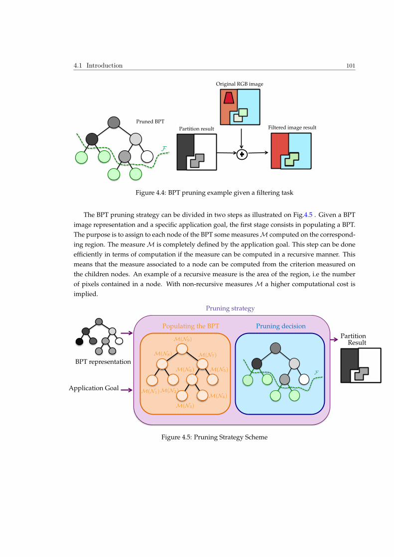
4.1 Introduction 101
Original RGB image
Filtered image result
F
Pruned BPT
Partition result
Figure 4.4: BPT pruning example given a filtering task
The BPT pruning strategy can be divided in two steps as illustrated on Fig.4.5 . Given a BPT
image representation and a specific application goal, the first stage consists in populating a BPT.
The purpose is to assign to each node of the BPT some measures M computed on the correspond-
ing region. The measure M is completely defined by the application goal. This step can be done
efficiently in terms of computation if the measure can be computed in a recursive manner. This
means that the measure associated to a node can be computed from the criterion measured on
the children nodes. An example of a recursive measure is the area of the region, i.e the number
of pixels contained in a node. With non-recursive measures M a higher computational cost is
implied.
PartitionResult
Pruning strategy
Pruning decisionPopulating the BPT
M(N8)
M(N2)M(N1)
M(N9)
M(N7)
M(N6) M(N5)
M(N4)
M(N3)
F
Application Goal
BPT representation
Figure 4.5: Pruning Strategy Scheme
102 Chapter 4. BPT Pruning Strategies
According to this first step, the second pruning stage is the definition of a function F which
analyzes the node measures in order to take the decision to preserve or to remove it. In the case
of an increasing function F , the pruning decision can be easily taken. An increasing function F
assessed on a region represented by a BPT node is increasing if: 8R1 R2 =) F(R1) F(R2).
Consequently, if a node has to be removed, their corresponding descendant have to be removed
as well. Contrarily, in the case of non-increasing F function, the pruning decision may be more
complex. In this case, two simple strategies are known as the minimum and the maximum deci-
sion. In the minimum decision, a node is preserved if and only if all its ancestors also have to be
preserved. Contrarily, the maximum decision corresponds to the dual behavior. Thus, a node is
removed if and only if all its descendant nodes also have to be removed. The choice is also related
to the tree analysis which can follow a bottom-up or a top-down strategy.
Following the strategy described in Fig.4.5, different pruning strategies are presented in the next
Sections. Firstly, a supervised pruning strategy aiming at hyperspectral image classification is
proposed. According to the classification goal, a specific populating of the BPT node and the
corresponding pruning decision is detailed. For this application, some experimental results are
shown in order to illustrate the advantage of using a region-based representation for classifica-
tion.
Besides classification goal, a second purpose involving the unsupervised segmentation of hyper-
spectral images is proposed in Sec.4.3 and Sec.4.4. In this context, two different pruning strategies
are discussed. The first approach consists in minimizing an energy function on the BPT structure
to reach a global minimum of the cost associated to a partition. The second approach involves a
local pruning decision on the BPT branches.These pruning decisions are computed by interpret-
ing the BPT branch cut as a spectral graph partitioning problem.
Finally, an object detection pruning strategy is presented in Sec.4.5. In this last section, two exam-
ples of object recognition are proposed in an urban scene. Specifically, the roads and the building
of the HYDICE urban scene are detected by the proposed technique.
4.2 Supervised Hyperspectral Classification 103
4.2 Supervised Hyperspectral Classification
In this section, an example of tree processing aiming at classifying hyperspectral images is dis-
cussed. Hyperspectral image classification is the process of labeling a pixel or group of pixels on
the basis of their spectral and spatial similarities. In the past, the classification of hyperspectral
data has been tackled using various approaches (See Chapter 2). In the case of supervised tech-
niques, representative samples, called training samples, are used to specify the spectral attributes
of the different classes composing the scene. These class spectral features are then used by the
algorithm to perform the pixel labeling. To this end, the classification algorithm compares the
pixels of the image with the training samples features. Accordingly, a pixel is then labeled given
its spectral characteristics by the most likely class of the training samples. The complete labeled
image is known as a classification map.
According to the supervised classification objective, the goal of the pruning strategy described
here aims at constructing a classification map for hyperspectral data. Note that using the pruned
tree, a partition describing the pixel class assignment can be easily constructed by selecting the
leaf nodes of the resulting pruned tree (See Fig.4.2). The pruning strategy discussed in this sec-
tion corresponds to a bottom-up analysis of the BPT. The particular criterion used here directly
depends on our classification goal.
As it has been explained at the beginning of this chapter, the analysis of the tree consists of two
important steps. The first one computes and assigns specific region descriptors to each BPT node
N . The second step is the pruning decision whose task is to evaluate a cost associated to the
region descriptors and eventually to decide where to prune the tree. In this classification context,
both steps are explained in the following sections.
4.2.1 Populating the BPT
Given the classification aim, the main information, or node descriptor, to define our pruning in-
volves the class probability distribution PN . This probability distribution is a vector containing
the probabilities that the node belongs to each class Ci. The reliable estimation of these probabil-
ities is a very challenging task [3]. This is due to the small number of training samples and the
high number of features.
To address this issue, class probabilities are estimated in a supervised way by using a multi-class
classifier. From our knowledge, the most popular discriminative classifier in the hyperspectral
image community is the support vector machines classifier (SVM), which is characterized by its
ability to effectively deal with large input spaces (and to produce sparse solutions) using limited
training samples. This classifier has proved to be well suited for the classification of hyperspectral
data [1] [4][5] [6].
As SVMs is a supervised algorithm [68], the kernel parameters should be computed first using
a training step. Here, the SVM training is done by using some leaf nodes which correspond to
single spectra. The selection of these nodes directly depends on the available ground truth. The
kernel function constructed during the training process enables to map an input spectrum to a
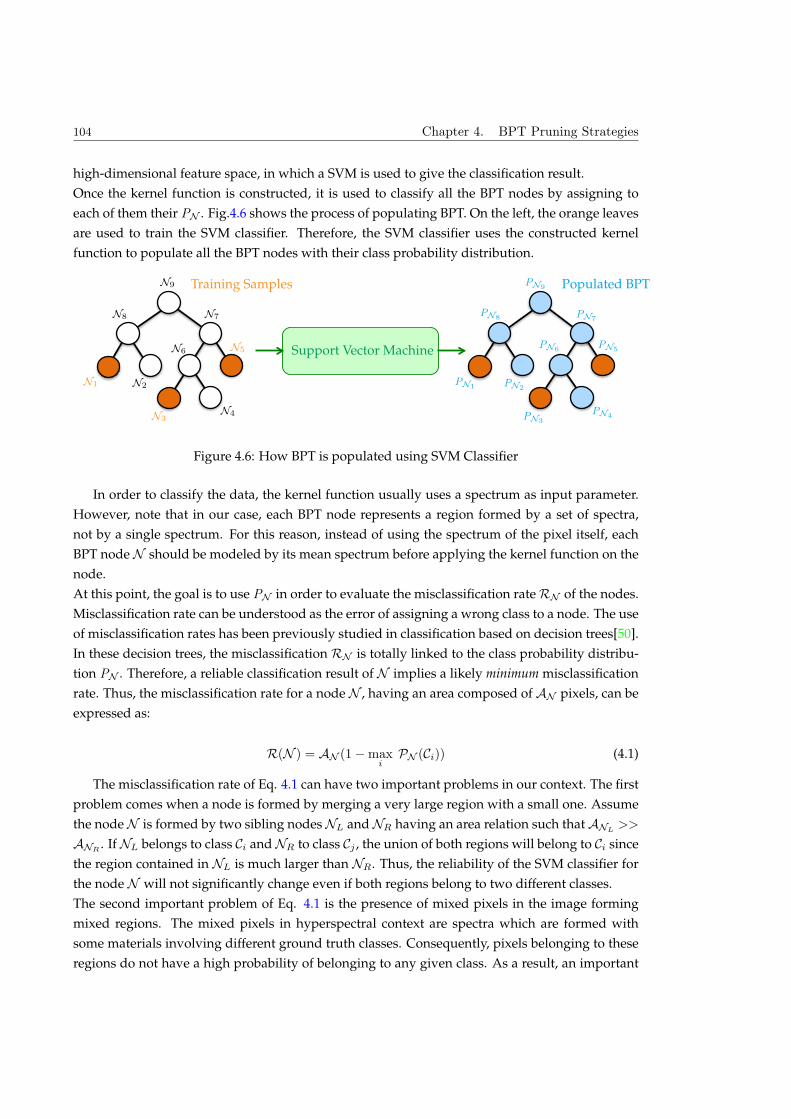
104 Chapter 4. BPT Pruning Strategies
high-dimensional feature space, in which a SVM is used to give the classification result.
Once the kernel function is constructed, it is used to classify all the BPT nodes by assigning to
each of them their PN . Fig.4.6 shows the process of populating BPT. On the left, the orange leaves
are used to train the SVM classifier. Therefore, the SVM classifier uses the constructed kernel
function to populate all the BPT nodes with their class probability distribution.
Support Vector Machine
Training Samples Populated BPT
N8
N2N1
N9
N7
N6N5
N4N3
PN8
PN2PN1
PN9
PN7
PN6PN5
PN4PN3
Figure 4.6: How BPT is populated using SVM Classifier
In order to classify the data, the kernel function usually uses a spectrum as input parameter.
However, note that in our case, each BPT node represents a region formed by a set of spectra,
not by a single spectrum. For this reason, instead of using the spectrum of the pixel itself, each
BPT node N should be modeled by its mean spectrum before applying the kernel function on the
node.
At this point, the goal is to use PN in order to evaluate the misclassification rate RN of the nodes.
Misclassification rate can be understood as the error of assigning a wrong class to a node. The use
of misclassification rates has been previously studied in classification based on decision trees[50].
In these decision trees, the misclassification RN is totally linked to the class probability distribu-
tion PN . Therefore, a reliable classification result of N implies a likely minimum misclassification
rate. Thus, the misclassification rate for a node N , having an area composed of AN pixels, can be
expressed as:
R(N ) = AN (1−maxi
PN (Ci)) (4.1)
The misclassification rate of Eq. 4.1 can have two important problems in our context. The first
problem comes when a node is formed by merging a very large region with a small one. Assume
the node N is formed by two sibling nodes NL and NR having an area relation such that ANL>>
ANR. If NL belongs to class Ci and NR to class Cj , the union of both regions will belong to Ci since
the region contained in NL is much larger than NR. Thus, the reliability of the SVM classifier for
the node N will not significantly change even if both regions belong to two different classes.
The second important problem of Eq. 4.1 is the presence of mixed pixels in the image forming
mixed regions. The mixed pixels in hyperspectral context are spectra which are formed with
some materials involving different ground truth classes. Consequently, pixels belonging to these
regions do not have a high probability of belonging to any given class. As a result, an important
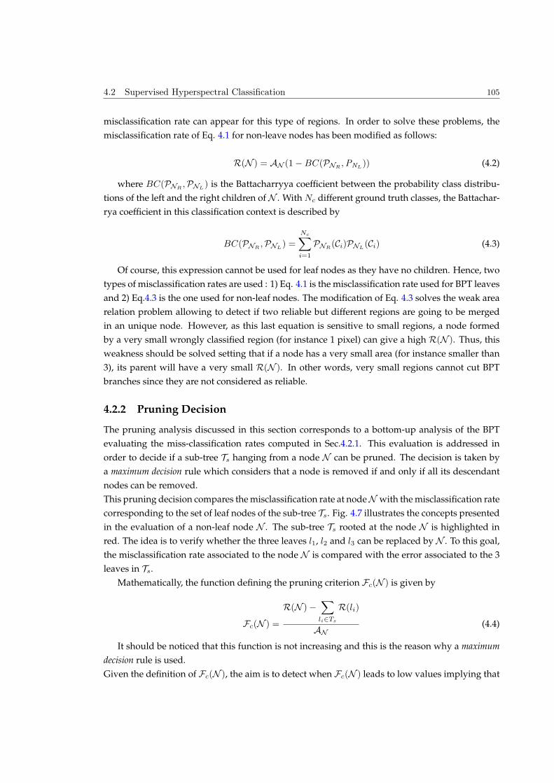
4.2 Supervised Hyperspectral Classification 105
misclassification rate can appear for this type of regions. In order to solve these problems, the
misclassification rate of Eq. 4.1 for non-leave nodes has been modified as follows:
R(N ) = AN (1−BC(PNR,PNL
)) (4.2)
where BC(PNR,PNL
) is the Battacharryya coefficient between the probability class distribu-
tions of the left and the right children of N . With Nc different ground truth classes, the Battachar-
rya coefficient in this classification context is described by
BC(PNR,PNL
) =
NcX
i=1
PNR(Ci)PNL
(Ci) (4.3)
Of course, this expression cannot be used for leaf nodes as they have no children. Hence, two
types of misclassification rates are used : 1) Eq. 4.1 is the misclassification rate used for BPT leaves
and 2) Eq.4.3 is the one used for non-leaf nodes. The modification of Eq. 4.3 solves the weak area
relation problem allowing to detect if two reliable but different regions are going to be merged
in an unique node. However, as this last equation is sensitive to small regions, a node formed
by a very small wrongly classified region (for instance 1 pixel) can give a high R(N ). Thus, this
weakness should be solved setting that if a node has a very small area (for instance smaller than
3), its parent will have a very small R(N ). In other words, very small regions cannot cut BPT
branches since they are not considered as reliable.
4.2.2 Pruning Decision
The pruning analysis discussed in this section corresponds to a bottom-up analysis of the BPT
evaluating the miss-classification rates computed in Sec.4.2.1. This evaluation is addressed in
order to decide if a sub-tree Ts hanging from a node N can be pruned. The decision is taken by
a maximum decision rule which considers that a node is removed if and only if all its descendant
nodes can be removed.
This pruning decision compares the misclassification rate at node N with the misclassification rate
corresponding to the set of leaf nodes of the sub-tree Ts. Fig. 4.7 illustrates the concepts presented
in the evaluation of a non-leaf node N . The sub-tree Ts rooted at the node N is highlighted in
red. The idea is to verify whether the three leaves l1, l2 and l3 can be replaced by N . To this goal,
the misclassification rate associated to the node N is compared with the error associated to the 3
leaves in Ts.
Mathematically, the function defining the pruning criterion Fc(N ) is given by
Fc(N ) =
R(N )−X
li2Ts
R(li)
AN(4.4)
It should be noticed that this function is not increasing and this is the reason why a maximum
decision rule is used.
Given the definition of Fc(N ), the aim is to detect when Fc(N ) leads to low values implying that
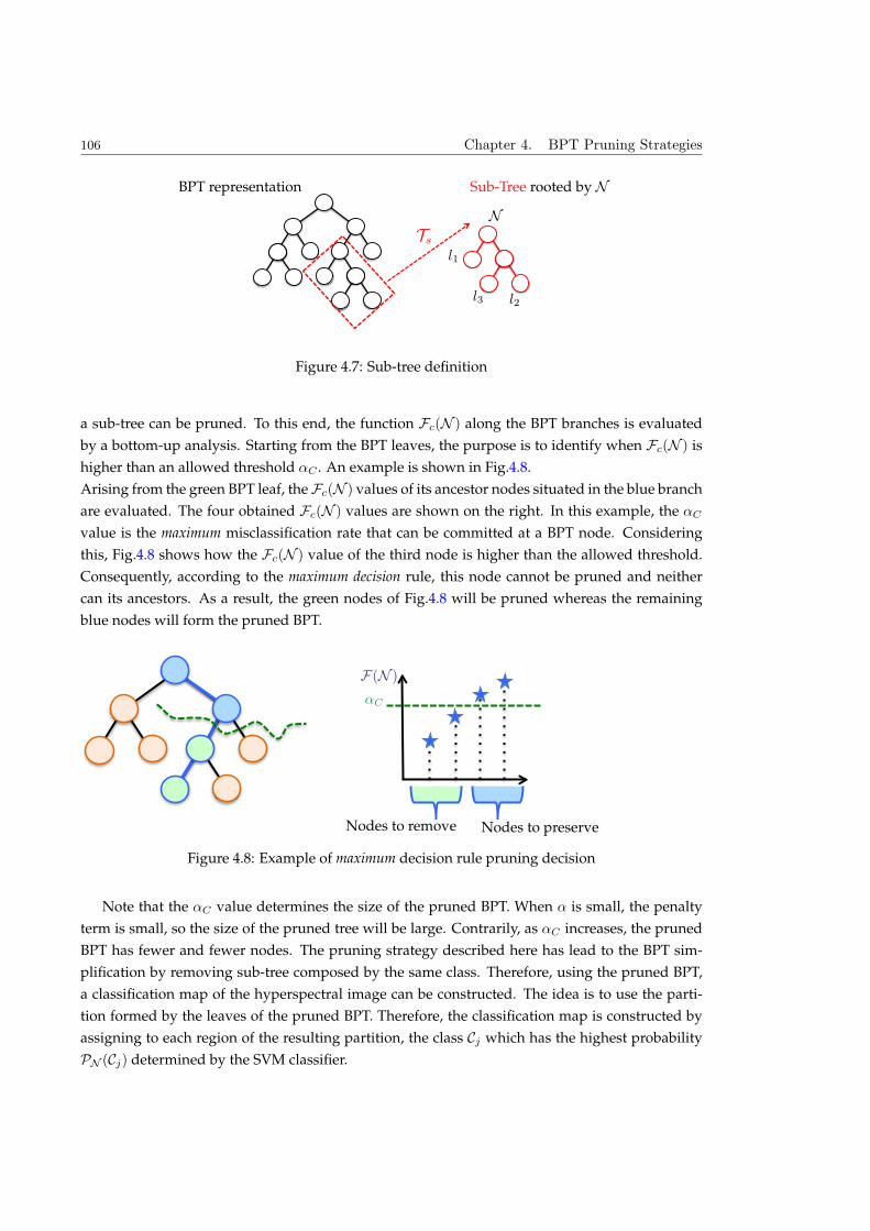
106 Chapter 4. BPT Pruning Strategies
Sub-Tree rooted by NBPT representation
Ts
N
l1
l2l3
Figure 4.7: Sub-tree definition
a sub-tree can be pruned. To this end, the function Fc(N ) along the BPT branches is evaluated
by a bottom-up analysis. Starting from the BPT leaves, the purpose is to identify when Fc(N ) is
higher than an allowed threshold ↵C . An example is shown in Fig.4.8.
Arising from the green BPT leaf, the Fc(N ) values of its ancestor nodes situated in the blue branch
are evaluated. The four obtained Fc(N ) values are shown on the right. In this example, the ↵C
value is the maximum misclassification rate that can be committed at a BPT node. Considering
this, Fig.4.8 shows how the Fc(N ) value of the third node is higher than the allowed threshold.
Consequently, according to the maximum decision rule, this node cannot be pruned and neither
can its ancestors. As a result, the green nodes of Fig.4.8 will be pruned whereas the remaining
blue nodes will form the pruned BPT.
F(N )
↵C
Nodes to remove Nodes to preserve
Figure 4.8: Example of maximum decision rule pruning decision
Note that the ↵C value determines the size of the pruned BPT. When ↵ is small, the penalty
term is small, so the size of the pruned tree will be large. Contrarily, as ↵C increases, the pruned
BPT has fewer and fewer nodes. The pruning strategy described here has lead to the BPT sim-
plification by removing sub-tree composed by the same class. Therefore, using the pruned BPT,
a classification map of the hyperspectral image can be constructed. The idea is to use the parti-
tion formed by the leaves of the pruned BPT. Therefore, the classification map is constructed by
assigning to each region of the resulting partition, the class Cj which has the highest probability
PN (Cj) determined by the SVM classifier.
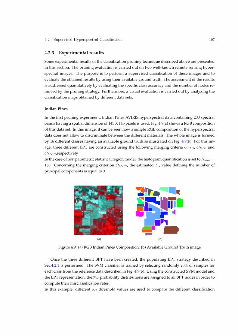
4.2 Supervised Hyperspectral Classification 107
4.2.3 Experimental results
Some experimental results of the classification pruning technique described above are presented
in this section. The pruning evaluation is carried out on two well-known remote sensing hyper-
spectral images. The purpose is to perform a supervised classification of these images and to
evaluate the obtained results by using their available ground truth. The assessment of the results
is addressed quantitatively by evaluating the specific class accuracy and the number of nodes re-
moved by the pruning strategy. Furthermore, a visual evaluation is carried out by analyzing the
classification maps obtained by different data sets.
Indian Pines
In the first pruning experiment, Indian Pines AVIRIS hyperspectral data containing 200 spectral
bands having a spatial dimension of 145 X 145 pixels is used. Fig. 4.9(a) shows a RGB composition
of this data set. In this image, it can be seen how a simple RGB composition of the hyperspectral
data does not allow to discriminate between the different materials. The whole image is formed
by 16 different classes having an available ground truth as illustrated on Fig. 4.9(b). For this im-
age, three different BPT are constructed using the following merging criteria OSID, ODIF and
OMDS ,respectively.
In the case of non parametric statistical region model, the histogram quantification is set to Nbins =
150. Concerning the merging criterion OMDS , the estimated Ds value defining the number of
principal components is equal to 3.
!! ! !!!!"#$ $ $ $
(a) (b)
Figure 4.9: (a) RGB Indian Pines Composition. (b) Available Ground Truth image
Once the three different BPT have been created, the populating BPT strategy described in
Sec.4.2.1 is performed. The SVM classifier is trained by selecting randomly 20% of samples for
each class from the reference data described in Fig. 4.9(b). Using the constructed SVM model and
the BPT representation, the PN probability distributions are assigned to all BPT nodes in order to
compute their misclassification rates.
In this example, different ↵C threshold values are used to compare the different classification
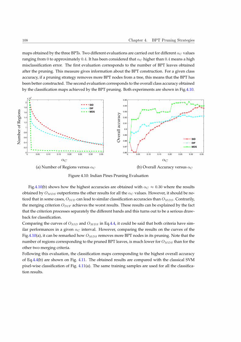
108 Chapter 4. BPT Pruning Strategies
maps obtained by the three BPTs. Two different evaluations are carried out for different ↵C values
ranging from 0 to approximately 0.4. It has been considered that ↵C higher than 0.4 means a high
misclassification error. The first evaluation corresponds to the number of BPT leaves obtained
after the pruning. This measure gives information about the BPT construction. For a given class
accuracy, if a pruning strategy removes more BPT nodes from a tree, this means that the BPT has
been better constructed. The second evaluation corresponds to the overall class accuracy obtained
by the classification maps achieved by the BPT pruning. Both experiments are shown in Fig.4.10.
0 0.05 0.10 0.15 0.20 0.25 0.30 0.350
0.2
0.4
0.6
0.8
1
1.2
1.4
1.6
1.8
2
x 104
0 0.05 0.10 0.15 0.20 0.25 0.30 0.350.86
0.87
0.88
0.89
0.9
0.91
0.92
0.93
0.94
0.95
SID
DIF
MDS
SID
DIF
MDS
Ov
eral
lac
cura
cy
(b) Overall Accuracy versus ↵C
αC
(a) Number of Regions versus ↵C
αC
Nu
mb
ero
fR
egio
ns
Figure 4.10: Indian Pines Pruning Evaluation
Fig.4.10(b) shows how the highest accuracies are obtained with ↵C 0.30 where the results
obtained by OMDS outperforms the other results for all the ↵C values. However, it should be no-
ticed that in some cases, OSID can lead to similar classification accuracies than OMDS . Contrarily,
the merging criterion ODIF achieves the worst results. These results can be explained by the fact
that the criterion processes separately the different bands and this turns out to be a serious draw-
back for classification.
Comparing the curves of OSID and OMDS in Eq.4.4, it could be said that both criteria have sim-
ilar performances in a given ↵C interval. However, comparing the results on the curves of the
Fig.4.10(a), it can be remarked how OMDS removes more BPT nodes in its pruning. Note that the
number of regions corresponding to the pruned BPT leaves, is much lower for OMDS than for the
other two merging criteria.
Following this evaluation, the classification maps corresponding to the highest overall accuracy
of Eq.4.4(b) are shown on Fig. 4.11. The obtained results are compared with the classical SVM
pixel-wise classification of Fig. 4.11(a). The same training samples are used for all the classifica-
tion results.
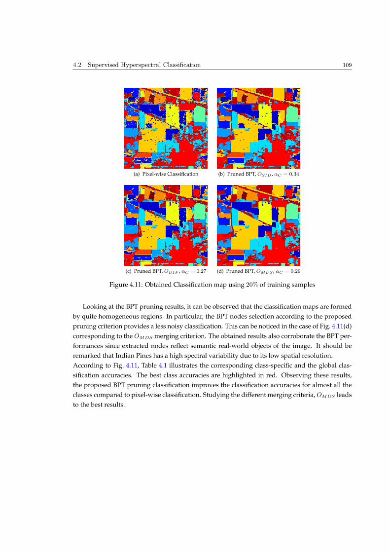
4.2 Supervised Hyperspectral Classification 109
(a) Pixel-wise Classification (b) Pruned BPT, OSID , αC = 0.34
(c) Pruned BPT, ODIF , αC = 0.27 (d) Pruned BPT, OMDS , αC = 0.29
Figure 4.11: Obtained Classification map using 20% of training samples
Looking at the BPT pruning results, it can be observed that the classification maps are formed
by quite homogeneous regions. In particular, the BPT nodes selection according to the proposed
pruning criterion provides a less noisy classification. This can be noticed in the case of Fig. 4.11(d)
corresponding to the OMDS merging criterion. The obtained results also corroborate the BPT per-
formances since extracted nodes reflect semantic real-world objects of the image. It should be
remarked that Indian Pines has a high spectral variability due to its low spatial resolution.
According to Fig. 4.11, Table 4.1 illustrates the corresponding class-specific and the global clas-
sification accuracies. The best class accuracies are highlighted in red. Observing these results,
the proposed BPT pruning classification improves the classification accuracies for almost all the
classes compared to pixel-wise classification. Studying the different merging criteria, OMDS leads
to the best results.
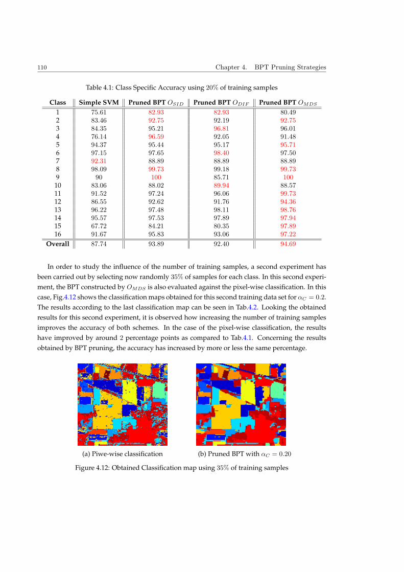
110 Chapter 4. BPT Pruning Strategies
Table 4.1: Class Specific Accuracy using 20% of training samples
Class Simple SVM Pruned BPT OSID Pruned BPT ODIF Pruned BPT OMDS
1 75.61 82.93 82.93 80.492 83.46 92.75 92.19 92.753 84.35 95.21 96.81 96.014 76.14 96.59 92.05 91.485 94.37 95.44 95.17 95.716 97.15 97.65 98.40 97.507 92.31 88.89 88.89 88.898 98.09 99.73 99.18 99.739 90 100 85.71 10010 83.06 88.02 89.94 88.5711 91.52 97.24 96.06 99.7312 86.55 92.62 91.76 94.3613 96.22 97.48 98.11 98.7614 95.57 97.53 97.89 97.9415 67.72 84.21 80.35 97.8916 91.67 95.83 93.06 97.22
Overall 87.74 93.89 92.40 94.69
In order to study the influence of the number of training samples, a second experiment has
been carried out by selecting now randomly 35% of samples for each class. In this second experi-
ment, the BPT constructed by OMDS is also evaluated against the pixel-wise classification. In this
case, Fig.4.12 shows the classification maps obtained for this second training data set for ↵C = 0.2.
The results according to the last classification map can be seen in Tab.4.2. Looking the obtained
results for this second experiment, it is observed how increasing the number of training samples
improves the accuracy of both schemes. In the case of the pixel-wise classification, the results
have improved by around 2 percentage points as compared to Tab.4.1. Concerning the results
obtained by BPT pruning, the accuracy has increased by more or less the same percentage.
(a) (b)(a) Piwe-wise classification (b) Pruned BPT with ↵C = 0.20
Figure 4.12: Obtained Classification map using 35% of training samples
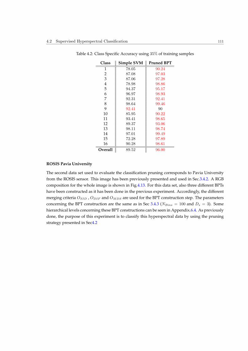
4.2 Supervised Hyperspectral Classification 111
Table 4.2: Class Specific Accuracy using 35% of training samples
Class Simple SVM Pruned BPT
1 78.05 90.242 87.08 97.033 87.06 97.284 78.98 98.865 94.37 95.176 96.97 98.937 92.31 92.418 98.64 99.469 92.41 90
10 85.95 90.2211 93.41 98.6512 89.37 93.0613 98.11 98.7414 97.01 99.4915 72.28 97.8916 90.28 98.61
Overall 89.52 96.00
ROSIS Pavia University
The second data set used to evaluate the classification pruning corresponds to Pavia University
from the ROSIS sensor. This image has been previously presented and used in Sec.3.4.2. A RGB
composition for the whole image is shown in Fig.4.13. For this data set, also three different BPTs
have been constructed as it has been done in the previous experiment. Accordingly, the different
merging criteria OSID , ODIF and OMDS are used for the BPT construction step. The parameters
concerning the BPT construction are the same as in Sec 3.4.3 (NBins = 100 and Ds = 3). Some
hierarchical levels concerning these BPT constructions can be seen in Appendix.6.4. As previously
done, the purpose of this experiment is to classify this hyperspectral data by using the pruning
strategy presented in Sec4.2
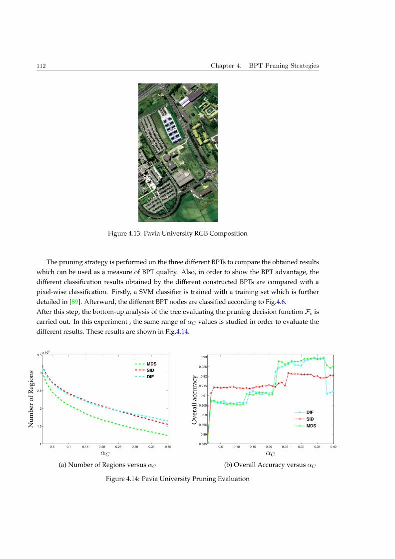
112 Chapter 4. BPT Pruning Strategies
(a)Figure 4.13: Pavia University RGB Composition
The pruning strategy is performed on the three different BPTs to compare the obtained results
which can be used as a measure of BPT quality. Also, in order to show the BPT advantage, the
different classification results obtained by the different constructed BPTs are compared with a
pixel-wise classification. Firstly, a SVM classifier is trained with a training set which is further
detailed in [89]. Afterward, the different BPT nodes are classified according to Fig.4.6.
After this step, the bottom-up analysis of the tree evaluating the pruning decision function Fc is
carried out. In this experiment , the same range of ↵C values is studied in order to evaluate the
different results. These results are shown in Fig.4.14.
0.5 0.1 0.15 0.20 0.25 0.30 0.35 0.401
1.5
2
2.5
3
3.5x 10
4
0.5 0.10 0.15 0.20 0.25 0.30 0.35 0.400.885
0.89
0.895
0.9
0.905
0.91
0.915
0.92
0.925
0.93
MDS
SID
DIF
DIF
SID
MDS
Ov
eral
lac
cura
cy
(b) Overall Accuracy versus ↵C
αC
(a) Number of Regions versus ↵C
αC
Nu
mb
ero
fR
egio
ns
Figure 4.14: Pavia University Pruning Evaluation
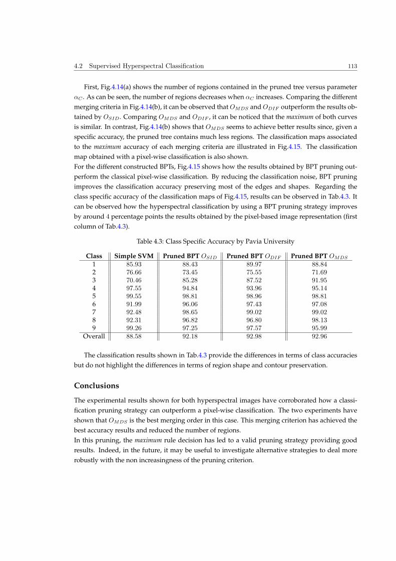
4.2 Supervised Hyperspectral Classification 113
First, Fig.4.14(a) shows the number of regions contained in the pruned tree versus parameter
↵C . As can be seen, the number of regions decreases when ↵C increases. Comparing the different
merging criteria in Fig.4.14(b), it can be observed that OMDS and ODIF outperform the results ob-
tained by OSID. Comparing OMDS and ODIF , it can be noticed that the maximum of both curves
is similar. In contrast, Fig.4.14(b) shows that OMDS seems to achieve better results since, given a
specific accuracy, the pruned tree contains much less regions. The classification maps associated
to the maximum accuracy of each merging criteria are illustrated in Fig.4.15. The classification
map obtained with a pixel-wise classification is also shown.
For the different constructed BPTs, Fig.4.15 shows how the results obtained by BPT pruning out-
perform the classical pixel-wise classification. By reducing the classification noise, BPT pruning
improves the classification accuracy preserving most of the edges and shapes. Regarding the
class specific accuracy of the classification maps of Fig.4.15, results can be observed in Tab.4.3. It
can be observed how the hyperspectral classification by using a BPT pruning strategy improves
by around 4 percentage points the results obtained by the pixel-based image representation (first
column of Tab.4.3).
Table 4.3: Class Specific Accuracy by Pavia University
Class Simple SVM Pruned BPT OSID Pruned BPT ODIF Pruned BPT OMDS
1 85.93 88.43 89.97 88.842 76.66 73.45 75.55 71.693 70.46 85.28 87.52 91.954 97.55 94.84 93.96 95.145 99.55 98.81 98.96 98.816 91.99 96.06 97.43 97.087 92.48 98.65 99.02 99.028 92.31 96.82 96.80 98.139 99.26 97.25 97.57 95.99
Overall 88.58 92.18 92.98 92.96
The classification results shown in Tab.4.3 provide the differences in terms of class accuracies
but do not highlight the differences in terms of region shape and contour preservation.
Conclusions
The experimental results shown for both hyperspectral images have corroborated how a classi-
fication pruning strategy can outperform a pixel-wise classification. The two experiments have
shown that OMDS is the best merging order in this case. This merging criterion has achieved the
best accuracy results and reduced the number of regions.
In this pruning, the maximum rule decision has led to a valid pruning strategy providing good
results. Indeed, in the future, it may be useful to investigate alternative strategies to deal more
robustly with the non increasingness of the pruning criterion.
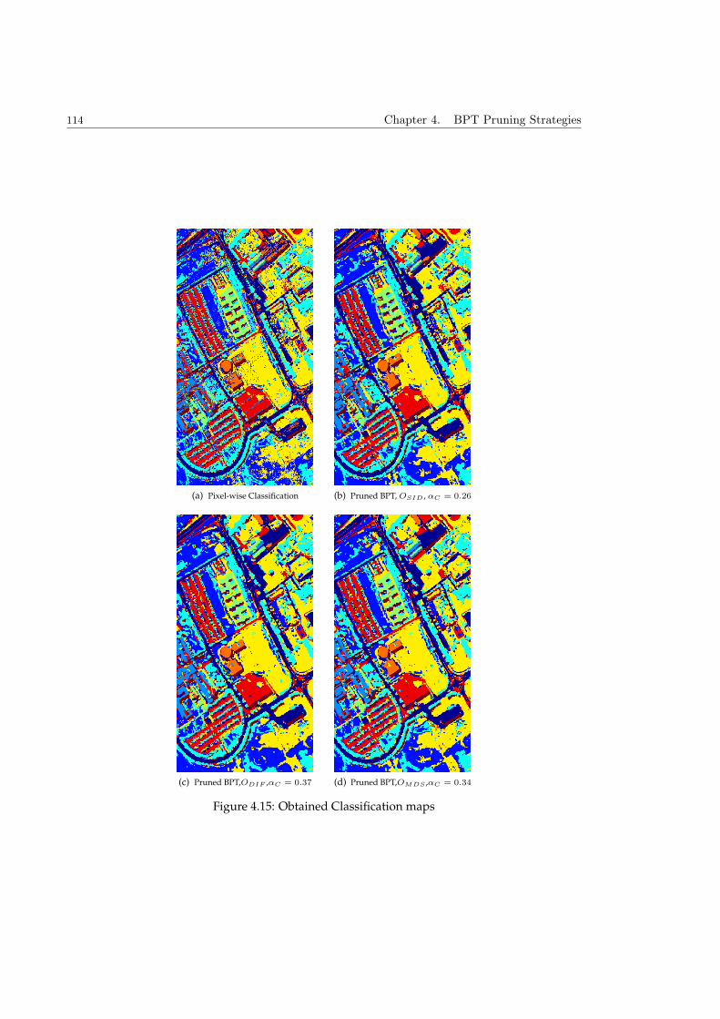
114 Chapter 4. BPT Pruning Strategies
(a) Pixel-wise Classification (b) Pruned BPT, OSID , αC = 0.26
(c) Pruned BPT,ODIF ,αC = 0.37 (d) Pruned BPT,OMDS ,αC = 0.34
Figure 4.15: Obtained Classification maps
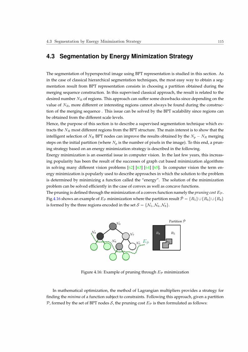
4.3 Segmentation by Energy Minimization Strategy 115
4.3 Segmentation by Energy Minimization Strategy
The segmentation of hyperspectral image using BPT representation is studied in this section. As
in the case of classical hierarchical segmentation techniques, the most easy way to obtain a seg-
mentation result from BPT representation consists in choosing a partition obtained during the
merging sequence construction. In this supervised classical approach, the result is related to the
desired number NR of regions. This approach can suffer some drawbacks since depending on the
value of NR, more different or interesting regions cannot always be found during the construc-
tion of the merging sequence . This issue can be solved by the BPT scalability since regions can
be obtained from the different scale levels.
Hence, the purpose of this section is to describe a supervised segmentation technique which ex-
tracts the NR most different regions from the BPT structure. The main interest is to show that the
intelligent selection of NR BPT nodes can improve the results obtained by the Np − NR merging
steps on the initial partition (where Np is the number of pixels in the image). To this end, a prun-
ing strategy based on an energy minimization strategy is described in the following.
Energy minimization is an essential issue in computer vision. In the last few years, this increas-
ing popularity has been the result of the successes of graph cut based minimization algorithms
in solving many different vision problems [62] [63] [64] [65]. In computer vision the term en-
ergy minimization is popularly used to describe approaches in which the solution to the problem
is determined by minimizing a function called the “energy”. The solution of the minimization
problem can be solved efficiently in the case of convex as well as concave functions.
The pruning is defined through the minimization of a convex function namely the pruning cost EP .
Fig.4.16 shows an example of EP minimization where the partition result P = R5[R6[R8
is formed by the three regions encoded in the set S = N5,N6,N8.
N6N5
EP
N7
N8
N9
R5
Partition P
R6
R8
Figure 4.16: Example of pruning through EP minimization
In mathematical optimization, the method of Lagrangian multipliers provides a strategy for
finding the minima of a function subject to constraints. Following this approach, given a partition
P , formed by the set of BPT nodes S , the pruning cost EP is then formulated as follows:
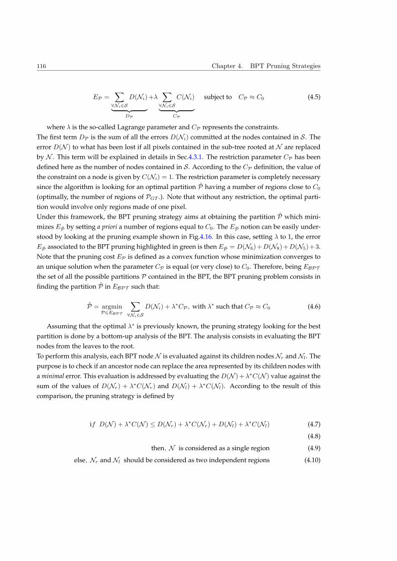
116 Chapter 4. BPT Pruning Strategies
EP =X
8Ni2S
D(Ni)
| z
DP
+λX
8Ni2S
C(Ni)
| z
CP
subject to CP C0 (4.5)
where λ is the so-called Lagrange parameter and CP represents the constraints.
The first term DP is the sum of all the errors D(Ni) committed at the nodes contained in S . The
error D(N ) to what has been lost if all pixels contained in the sub-tree rooted at N are replaced
by N . This term will be explained in details in Sec.4.3.1. The restriction parameter CP has been
defined here as the number of nodes contained in S . According to the CP definition, the value of
the constraint on a node is given by C(Ni) = 1. The restriction parameter is completely necessary
since the algorithm is looking for an optimal partition P having a number of regions close to C0
(optimally, the number of regions of PGT .). Note that without any restriction, the optimal parti-
tion would involve only regions made of one pixel.
Under this framework, the BPT pruning strategy aims at obtaining the partition P which mini-
mizes EP by setting a priori a number of regions equal to C0. The EP notion can be easily under-
stood by looking at the pruning example shown in Fig.4.16. In this case, setting λ to 1, the error
EP associated to the BPT pruning highlighted in green is then EP = D(N6)+D(N8)+D(N5)+3.
Note that the pruning cost EP is defined as a convex function whose minimization converges to
an unique solution when the parameter CP is equal (or very close) to C0. Therefore, being EBPT
the set of all the possible partitions P contained in the BPT, the BPT pruning problem consists in
finding the partition P in EBPT such that:
P = argminP2EBPT
X
8Ni2S
D(Ni) + λCP , with λ such that CP C0 (4.6)
Assuming that the optimal λ is previously known, the pruning strategy looking for the best
partition is done by a bottom-up analysis of the BPT. The analysis consists in evaluating the BPT
nodes from the leaves to the root.
To perform this analysis, each BPT node N is evaluated against its children nodes Nr and Nl. The
purpose is to check if an ancestor node can replace the area represented by its children nodes with
a minimal error. This evaluation is addressed by evaluating the D(N )+λC(N ) value against the
sum of the values of D(Nr) + λC(Nr) and D(Nl) + λC(Nl). According to the result of this
comparison, the pruning strategy is defined by
if D(N ) + λC(N ) D(Nr) + λC(Nr) +D(Nl) + λC(Nl) (4.7)
(4.8)
then, N is considered as a single region (4.9)
else, Nr and Nl should be considered as two independent regions (4.10)
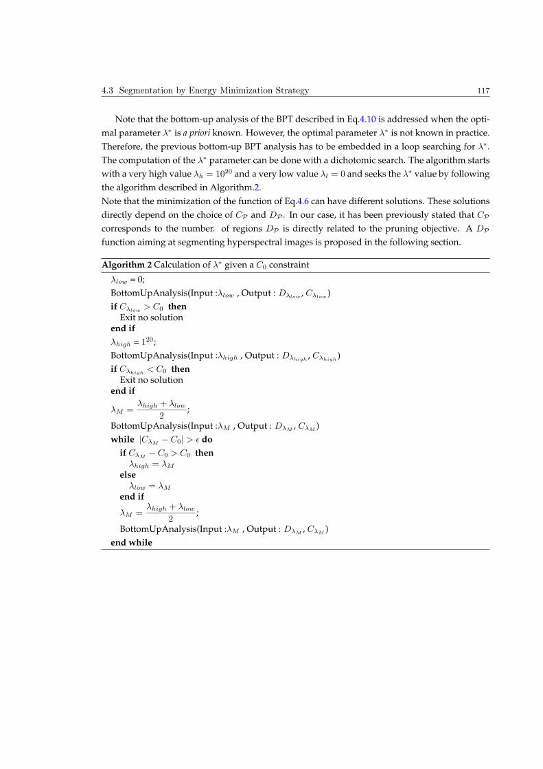
4.3 Segmentation by Energy Minimization Strategy 117
Note that the bottom-up analysis of the BPT described in Eq.4.10 is addressed when the opti-
mal parameter λ is a priori known. However, the optimal parameter λ is not known in practice.
Therefore, the previous bottom-up BPT analysis has to be embedded in a loop searching for λ.
The computation of the λ parameter can be done with a dichotomic search. The algorithm starts
with a very high value λh = 1020 and a very low value λl = 0 and seeks the λ value by following
the algorithm described in Algorithm.2.
Note that the minimization of the function of Eq.4.6 can have different solutions. These solutions
directly depend on the choice of CP and DP . In our case, it has been previously stated that CP
corresponds to the number. of regions DP is directly related to the pruning objective. A DP
function aiming at segmenting hyperspectral images is proposed in the following section.
Algorithm 2 Calculation of λ given a C0 constraint
λlow = 0;
BottomUpAnalysis(Input :λlow , Output : Dλlow, Cλlow
)
if Cλlow> C0 then
Exit no solutionend if
λhigh = 120;
BottomUpAnalysis(Input :λhigh , Output : Dλhigh, Cλhigh
)
if Cλhigh< C0 then
Exit no solutionend if
λM =λhigh + λlow
2;
BottomUpAnalysis(Input :λM , Output : DλM, CλM
)
while |CλM− C0| > do
if CλM− C0 > C0 then
λhigh = λM
elseλlow = λM
end if
λM =λhigh + λlow
2;
BottomUpAnalysis(Input :λM , Output : DλM, CλM
)
end while
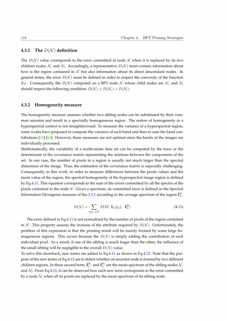
118 Chapter 4. BPT Pruning Strategies
4.3.1 The D(N ) definition
The D(N ) value corresponds to the error committed at node N when it is replaced by its two
children nodes Nr and Nl. Accordingly, a representative D(N ) must contain information about
how is the region contained in N but also information about its direct descendant nodes. In
general terms, the error D(N ) must be defined in order to respect the convexity of the function
EP . Consequently, the D(N ) computed on a BPT node N whose child nodes are Nr and Nl
should respect the following condition: D(N ) ≥ D(Nr) +D(Nl).
4.3.2 Homogeneity measure
The homogeneity measure assesses whether two sibling nodes can be substituted by their com-
mon ancestor and result in a spectrally homogeneous region. The notion of homogeneity in a
hyperspectral context is not straightforward. To measure the variance of a hyperspectral region,
some works have proposed to compute the variance of each band and then to sum the band con-
tributions [19] [69]. However, these measures are not optimal since the bands of the images are
individually processed.
Mathematically, the variability of a multivariate data set can be computed by the trace or the
determinant of the covariance matrix representing the relations between the components of the
set. In our case, the number of pixels in a region is usually not much larger than the spectral
dimension of the image. Thus, the estimation of the covariance matrix is especially challenging.
Consequently, in this work, in order to measure differences between the pixels values and the
mean value of the region, the spectral homogeneity of the hyperspectral image region is defined
by Eq.4.11. This equation corresponds to the sum of the errors committed by all the spectra of the
pixels contained in the node N . Given a spectrum, its committed error is defined as the Spectral
Information Divergence measure of Sec.3.3.1 according to the average spectrum of the region IRλ .
D(N ) =X
8pj 2N
SID( Iλ(pj), IRλ ) (4.11)
The error defined in Eq.4.11 is not normalized by the number of pixels of the region contained
in N . This property assures the increase of the attribute required by D(N ). Unfortunately, the
problem of this expression is that the pruning result will be mainly formed by some large ho-
mogeneous regions. This occurs because the D(N) is simply adding the contribution of each
individual pixel. As a result, if one of the sibling is much larger than the other, the influence of
the small sibling will be negligible in the overall D(N) value.
To solve this drawback, new terms are added to Eq.4.11 as shown in Eq.4.12. Note that the pur-
pose of the new terms of Eq.4.12 are to detect whether an ancestor node is formed by two different
children regions. In these second term, IRr
λ and IRl
λ are the mean spectrum of the sibling nodes Nr
and Nl. From Eq.4.12, it can be observed how each new term corresponds to the error committed
by a node Ni when all its pixels are replaced by the mean spectrum of its sibling node.
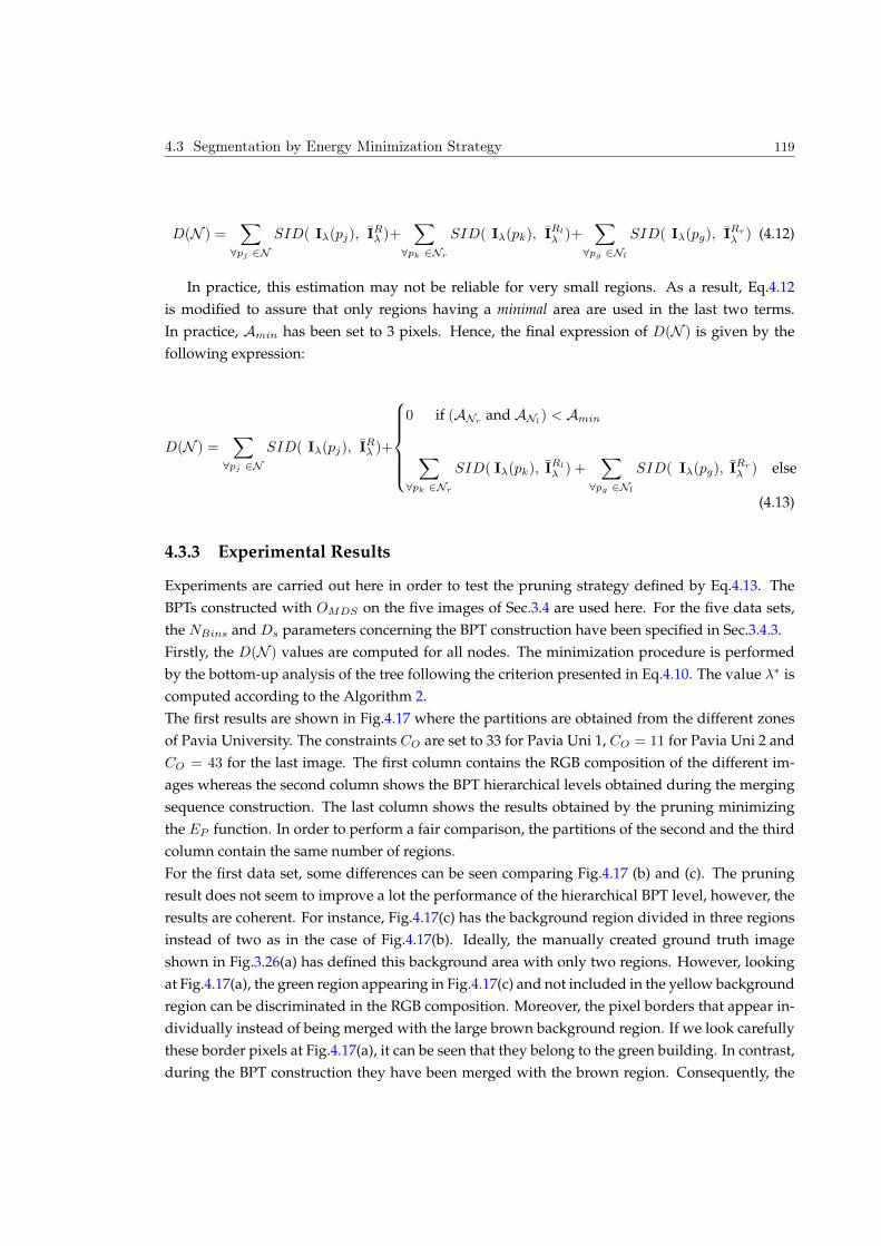
4.3 Segmentation by Energy Minimization Strategy 119
D(N ) =X
8pj 2N
SID( Iλ(pj), IRλ )+X
8pk 2Nr
SID( Iλ(pk), IRl
λ )+X
8pg 2Nl
SID( Iλ(pg), IRr
λ ) (4.12)
In practice, this estimation may not be reliable for very small regions. As a result, Eq.4.12
is modified to assure that only regions having a minimal area are used in the last two terms.
In practice, Amin has been set to 3 pixels. Hence, the final expression of D(N ) is given by the
following expression:
D(N ) =X
8pj 2N
SID( Iλ(pj), IRλ )+
8
>>>><
>>>>:
0 if (ANrand ANl
) < Amin
X
8pk 2Nr
SID( Iλ(pk), IRl
λ ) +X
8pg 2Nl
SID( Iλ(pg), IRr
λ ) else
(4.13)
4.3.3 Experimental Results
Experiments are carried out here in order to test the pruning strategy defined by Eq.4.13. The
BPTs constructed with OMDS on the five images of Sec.3.4 are used here. For the five data sets,
the NBins and Ds parameters concerning the BPT construction have been specified in Sec.3.4.3.
Firstly, the D(N ) values are computed for all nodes. The minimization procedure is performed
by the bottom-up analysis of the tree following the criterion presented in Eq.4.10. The value λ is
computed according to the Algorithm 2.
The first results are shown in Fig.4.17 where the partitions are obtained from the different zones
of Pavia University. The constraints CO are set to 33 for Pavia Uni 1, CO = 11 for Pavia Uni 2 and
CO = 43 for the last image. The first column contains the RGB composition of the different im-
ages whereas the second column shows the BPT hierarchical levels obtained during the merging
sequence construction. The last column shows the results obtained by the pruning minimizing
the EP function. In order to perform a fair comparison, the partitions of the second and the third
column contain the same number of regions.
For the first data set, some differences can be seen comparing Fig.4.17 (b) and (c). The pruning
result does not seem to improve a lot the performance of the hierarchical BPT level, however, the
results are coherent. For instance, Fig.4.17(c) has the background region divided in three regions
instead of two as in the case of Fig.4.17(b). Ideally, the manually created ground truth image
shown in Fig.3.26(a) has defined this background area with only two regions. However, looking
at Fig.4.17(a), the green region appearing in Fig.4.17(c) and not included in the yellow background
region can be discriminated in the RGB composition. Moreover, the pixel borders that appear in-
dividually instead of being merged with the large brown background region. If we look carefully
these border pixels at Fig.4.17(a), it can be seen that they belong to the green building. In contrast,
during the BPT construction they have been merged with the brown region. Consequently, the
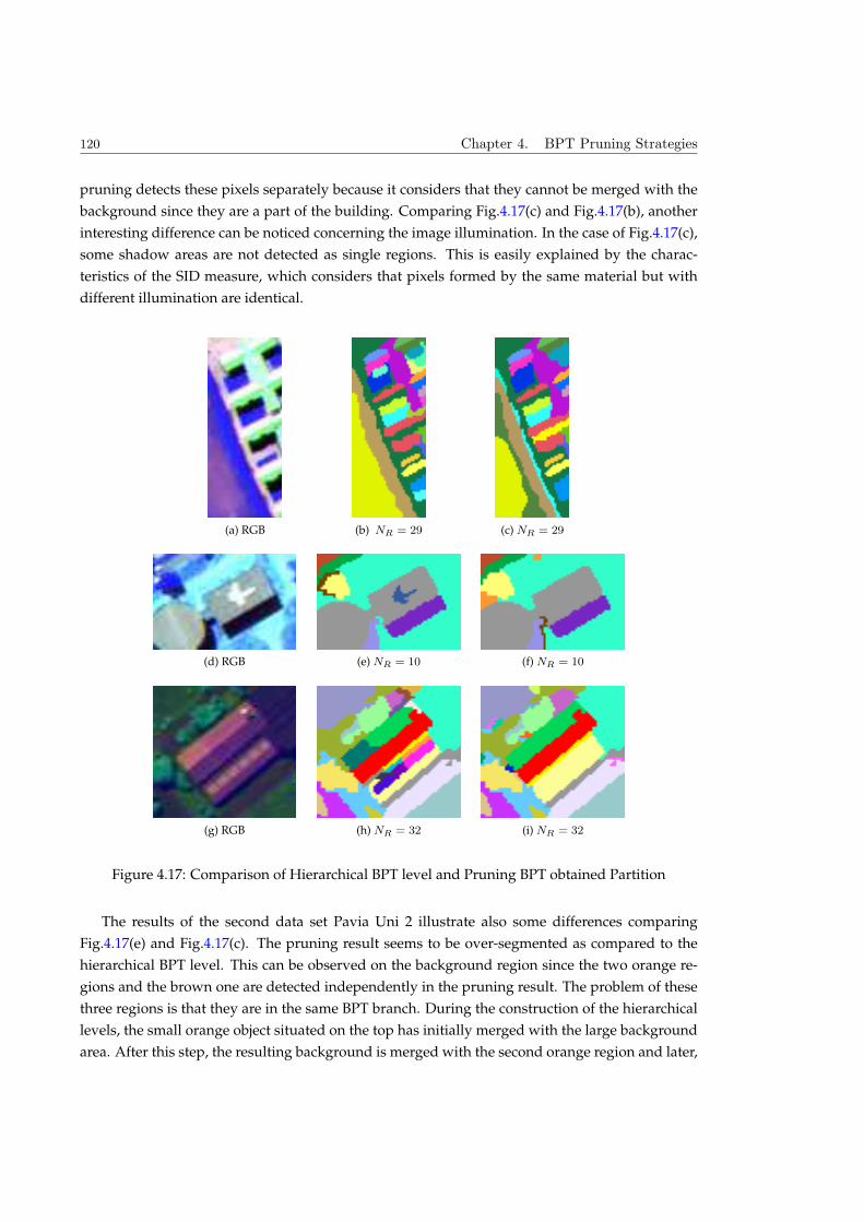
120 Chapter 4. BPT Pruning Strategies
pruning detects these pixels separately because it considers that they cannot be merged with the
background since they are a part of the building. Comparing Fig.4.17(c) and Fig.4.17(b), another
interesting difference can be noticed concerning the image illumination. In the case of Fig.4.17(c),
some shadow areas are not detected as single regions. This is easily explained by the charac-
teristics of the SID measure, which considers that pixels formed by the same material but with
different illumination are identical.
(a) RGB (b) NR = 29 (c) NR = 29
(d) RGB (e) NR = 10 (f) NR = 10
(g) RGB (h) NR = 32 (i) NR = 32
Figure 4.17: Comparison of Hierarchical BPT level and Pruning BPT obtained Partition
The results of the second data set Pavia Uni 2 illustrate also some differences comparing
Fig.4.17(e) and Fig.4.17(c). The pruning result seems to be over-segmented as compared to the
hierarchical BPT level. This can be observed on the background region since the two orange re-
gions and the brown one are detected independently in the pruning result. The problem of these
three regions is that they are in the same BPT branch. During the construction of the hierarchical
levels, the small orange object situated on the top has initially merged with the large background
area. After this step, the resulting background is merged with the second orange region and later,
4.3 Segmentation by Energy Minimization Strategy 121
it is merged with the brown region situated close to the building shadow. Therefore, as the small
orange object has been detected separately in the pruning result, the consequence is that the other
regions have not merged with the background region. This can seem an error of the pruning,
however, the detection of the small orange object is not wrong since this object really exists in
Fig.4.17(a). Hence, optimally, this small orange object should not be merged with the background
region before the other two background regions. On the other hand, it should be noticed that
the first merging concerning this small orange region during the BPT construction is explained
because of the scale threshold step of Sec.3.3.3. The area of this object is too small with respect
to the mean area of the regions forming its hierarchical level, then the merging of this object has
been forced.
In Fig.4.17(c), a problem can be detected on the pruning results since the large metallic object sit-
uated on the building roof has disappeared in the complete gray building region. This effect is
due to the definition of D(N ) that uses the Spectral Information Divergence (SID). Theoretically,
the complete region of the image formed by the roof building and the large metallic object must
have a large D(N ) value and consequently, these two regions should not merge. As the two re-
gions have a strong dissimilarity, the high value of D(N ) should come from the second term of
the Eq.4.13. However, after modeling the two regions by a mean spectrum, the SID between the
metallic region and the roof is not very high. Note that the first term concerning the parent ho-
mogeneity is not very high because most of the pixels form the building region. Accordingly, the
SID and the mean first order region model show some limitations in order to define an optimal
D(N ) descriptor at this example.
Going on with Fig.4.17 evaluation, the third data set also shows how the pruning technique ex-
tracts some small regions which have been merged previously with the background at the BPT
hierarchical levels. This can be observed on the right part of the figure, where some small regions
appear in the background area. At the same time, the pruning result shows how the main build-
ing is formed by less regions. Visually, the pruning result seems to achieve better results for this
third data set.
The same experiment is performed on the Pavia Center and HYDICE hyperspectral images. Set-
ting the constraint equal to CO = 25 for Pavia center and CO = 56 for HYDICE, the obtained re-
sults are shown in Fig.4.18. Looking at the first data set, it can be noticed how the background of
Pavia Center is formed by a single region in the pruning result. Besides, the pruning result shows
that the small blue region on the top-right corner has been retrieved by the pruning whereas
the same region does not appear in the hierarchical BPT level. The shadow effects can also be
remarked for this data set and also an over-segmentation issue concerning the vegetation area.
The problem of this over-segmented vegetation area is due to the fact that this region is strongly
textured. In the case of hierarchical levels, the statistical region model has taken into account
this texture characteristics. However, the pruning strategy is simply carried out by analyzing the
mean spectrum of the region. In addition, it can also be observed in the pruning result how some
small regions have cut the BPT branches because they are considered as not belonging to the large
vegetation area which is reasonable.
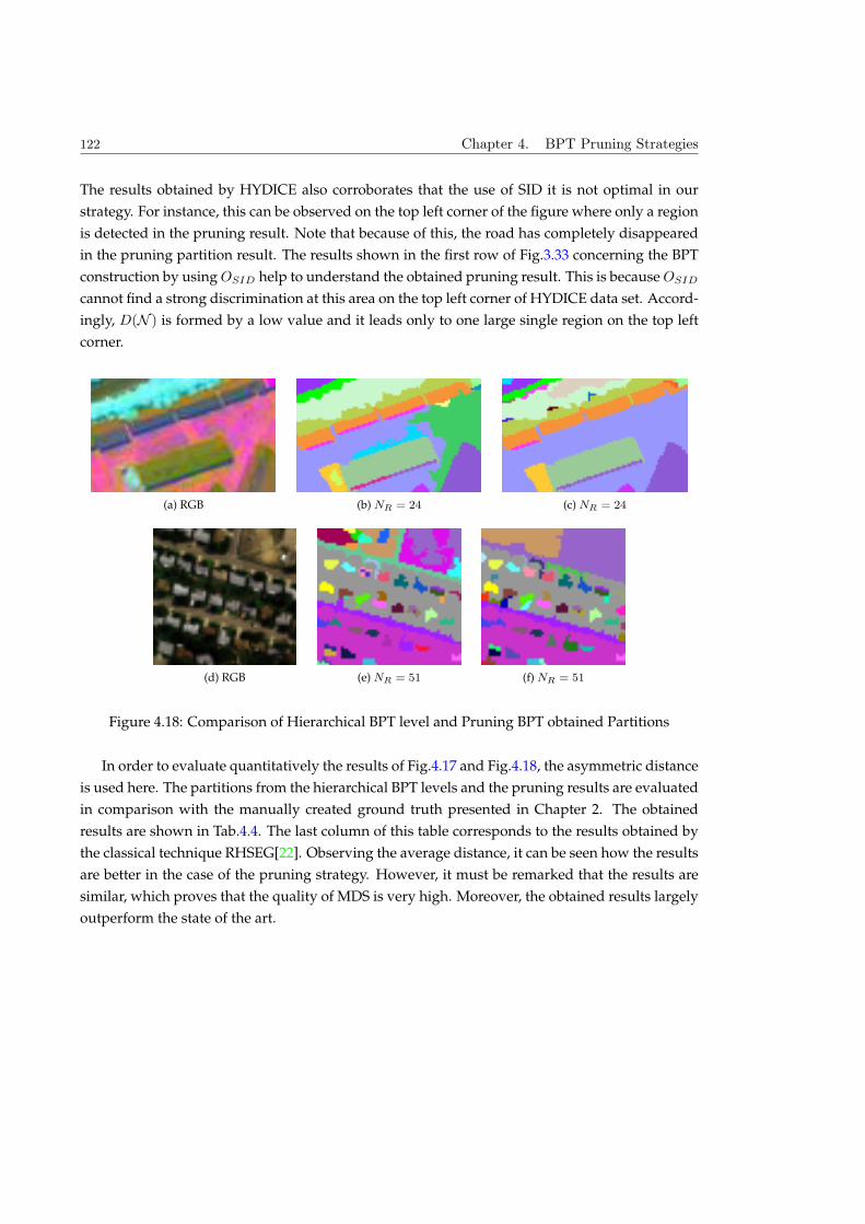
122 Chapter 4. BPT Pruning Strategies
The results obtained by HYDICE also corroborates that the use of SID it is not optimal in our
strategy. For instance, this can be observed on the top left corner of the figure where only a region
is detected in the pruning result. Note that because of this, the road has completely disappeared
in the pruning partition result. The results shown in the first row of Fig.3.33 concerning the BPT
construction by using OSID help to understand the obtained pruning result. This is because OSID
cannot find a strong discrimination at this area on the top left corner of HYDICE data set. Accord-
ingly, D(N ) is formed by a low value and it leads only to one large single region on the top left
corner.
(a) RGB (b) NR = 24 (c) NR = 24
(d) RGB (e) NR = 51 (f) NR = 51
Figure 4.18: Comparison of Hierarchical BPT level and Pruning BPT obtained Partitions
In order to evaluate quantitatively the results of Fig.4.17 and Fig.4.18, the asymmetric distance
is used here. The partitions from the hierarchical BPT levels and the pruning results are evaluated
in comparison with the manually created ground truth presented in Chapter 2. The obtained
results are shown in Tab.4.4. The last column of this table corresponds to the results obtained by
the classical technique RHSEG[22]. Observing the average distance, it can be seen how the results
are better in the case of the pruning strategy. However, it must be remarked that the results are
similar, which proves that the quality of MDS is very high. Moreover, the obtained results largely
outperform the state of the art.
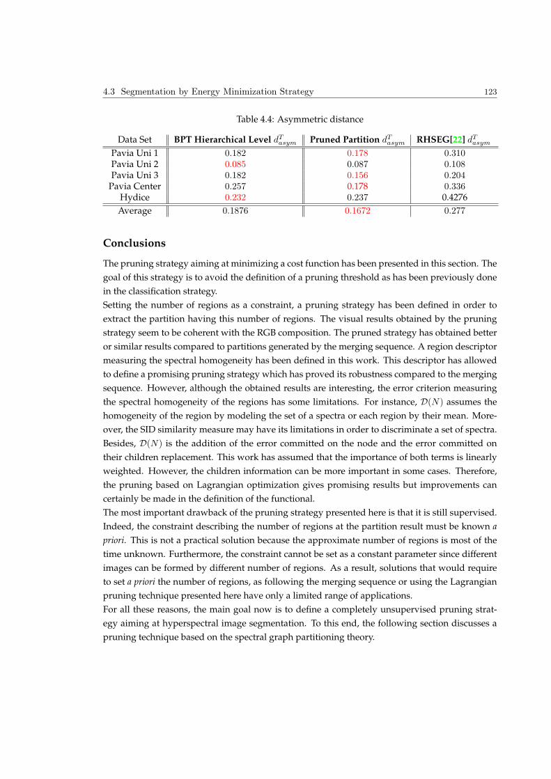
4.3 Segmentation by Energy Minimization Strategy 123
Table 4.4: Asymmetric distance
Data Set BPT Hierarchical Level dTasym Pruned Partition dTasym RHSEG[22] dTasymPavia Uni 1 0.182 0.178 0.310Pavia Uni 2 0.085 0.087 0.108Pavia Uni 3 0.182 0.156 0.204
Pavia Center 0.257 0.178 0.336Hydice 0.232 0.237 0.4276
Average 0.1876 0.1672 0.277
Conclusions
The pruning strategy aiming at minimizing a cost function has been presented in this section. The
goal of this strategy is to avoid the definition of a pruning threshold as has been previously done
in the classification strategy.
Setting the number of regions as a constraint, a pruning strategy has been defined in order to
extract the partition having this number of regions. The visual results obtained by the pruning
strategy seem to be coherent with the RGB composition. The pruned strategy has obtained better
or similar results compared to partitions generated by the merging sequence. A region descriptor
measuring the spectral homogeneity has been defined in this work. This descriptor has allowed
to define a promising pruning strategy which has proved its robustness compared to the merging
sequence. However, although the obtained results are interesting, the error criterion measuring
the spectral homogeneity of the regions has some limitations. For instance, D(N) assumes the
homogeneity of the region by modeling the set of a spectra or each region by their mean. More-
over, the SID similarity measure may have its limitations in order to discriminate a set of spectra.
Besides, D(N) is the addition of the error committed on the node and the error committed on
their children replacement. This work has assumed that the importance of both terms is linearly
weighted. However, the children information can be more important in some cases. Therefore,
the pruning based on Lagrangian optimization gives promising results but improvements can
certainly be made in the definition of the functional.
The most important drawback of the pruning strategy presented here is that it is still supervised.
Indeed, the constraint describing the number of regions at the partition result must be known a
priori. This is not a practical solution because the approximate number of regions is most of the
time unknown. Furthermore, the constraint cannot be set as a constant parameter since different
images can be formed by different number of regions. As a result, solutions that would require
to set a priori the number of regions, as following the merging sequence or using the Lagrangian
pruning technique presented here have only a limited range of applications.
For all these reasons, the main goal now is to define a completely unsupervised pruning strat-
egy aiming at hyperspectral image segmentation. To this end, the following section discusses a
pruning technique based on the spectral graph partitioning theory.
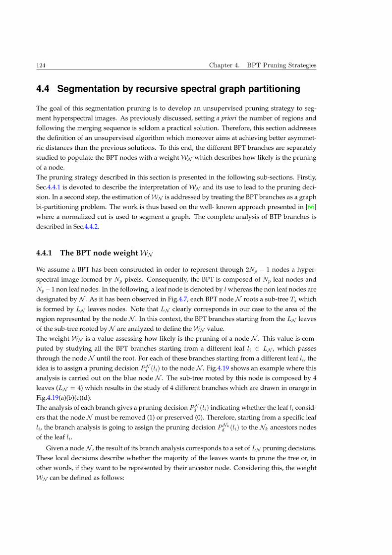
124 Chapter 4. BPT Pruning Strategies
4.4 Segmentation by recursive spectral graph partitioning
The goal of this segmentation pruning is to develop an unsupervised pruning strategy to seg-
ment hyperspectral images. As previously discussed, setting a priori the number of regions and
following the merging sequence is seldom a practical solution. Therefore, this section addresses
the definition of an unsupervised algorithm which moreover aims at achieving better asymmet-
ric distances than the previous solutions. To this end, the different BPT branches are separately
studied to populate the BPT nodes with a weight WN which describes how likely is the pruning
of a node.
The pruning strategy described in this section is presented in the following sub-sections. Firstly,
Sec.4.4.1 is devoted to describe the interpretation of WN and its use to lead to the pruning deci-
sion. In a second step, the estimation of WN is addressed by treating the BPT branches as a graph
bi-partitioning problem. The work is thus based on the well- known approach presented in [66]
where a normalized cut is used to segment a graph. The complete analysis of BTP branches is
described in Sec.4.4.2.
4.4.1 The BPT node weight WN
We assume a BPT has been constructed in order to represent through 2Np − 1 nodes a hyper-
spectral image formed by Np pixels. Consequently, the BPT is composed of Np leaf nodes and
Np−1 non leaf nodes. In the following, a leaf node is denoted by l whereas the non leaf nodes are
designated by N . As it has been observed in Fig.4.7, each BPT node N roots a sub-tree Ts which
is formed by LN leaves nodes. Note that LN clearly corresponds in our case to the area of the
region represented by the node N . In this context, the BPT branches starting from the LN leaves
of the sub-tree rooted by N are analyzed to define the WN value.
The weight WN is a value assessing how likely is the pruning of a node N . This value is com-
puted by studying all the BPT branches starting from a different leaf li 2 LN , which passes
through the node N until the root. For each of these branches starting from a different leaf li, the
idea is to assign a pruning decision PNd (li) to the node N . Fig.4.19 shows an example where this
analysis is carried out on the blue node N . The sub-tree rooted by this node is composed by 4
leaves (LN = 4) which results in the study of 4 different branches which are drawn in orange in
Fig.4.19(a)(b)(c)(d).
The analysis of each branch gives a pruning decision PNd (li) indicating whether the leaf li consid-
ers that the node N must be removed (1) or preserved (0). Therefore, starting from a specific leaf
li, the branch analysis is going to assign the pruning decision PNk
d (li) to the Nk ancestors nodes
of the leaf li.
Given a node N , the result of its branch analysis corresponds to a set of LN pruning decisions.
These local decisions describe whether the majority of the leaves wants to prune the tree or, in
other words, if they want to be represented by their ancestor node. Considering this, the weight
WN can be defined as follows:
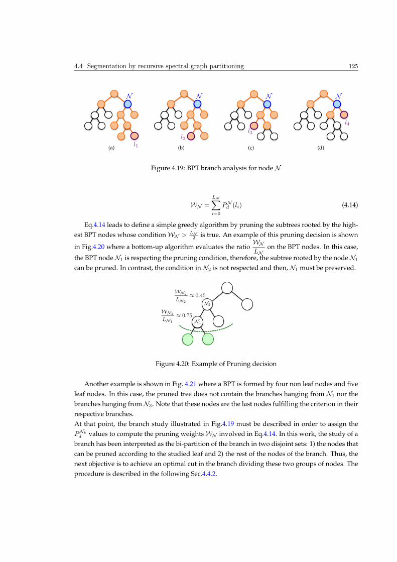
4.4 Segmentation by recursive spectral graph partitioning 125
(a)
N
l1 (b)
N
l2
(c)
N
l3
(d)
N
l4
Figure 4.19: BPT branch analysis for node N
WN =
LNX
i=0
PNd (li) (4.14)
Eq.4.14 leads to define a simple greedy algorithm by pruning the subtrees rooted by the high-
est BPT nodes whose condition WN > LN
2 is true. An example of this pruning decision is shown
in Fig.4.20 where a bottom-up algorithm evaluates the ratioWN
LNon the BPT nodes. In this case,
the BPT node N1 is respecting the pruning condition, therefore, the subtree rooted by the node N1
can be pruned. In contrast, the condition in N2 is not respected and then, N1 must be preserved.
WN2
LN2
≈ 0.45
WN1
LN1
≈ 0.75N1
N2
Figure 4.20: Example of Pruning decision
Another example is shown in Fig. 4.21 where a BPT is formed by four non leaf nodes and five
leaf nodes. In this case, the pruned tree does not contain the branches hanging from N1 nor the
branches hanging from N3. Note that these nodes are the last nodes fulfilling the criterion in their
respective branches.
At that point, the branch study illustrated in Fig.4.19 must be described in order to assign the
PNk
d values to compute the pruning weights WN involved in Eq.4.14. In this work, the study of a
branch has been interpreted as the bi-partition of the branch in two disjoint sets: 1) the nodes that
can be pruned according to the studied leaf and 2) the rest of the nodes of the branch. Thus, the
next objective is to achieve an optimal cut in the branch dividing these two groups of nodes. The
procedure is described in the following Sec.4.4.2.
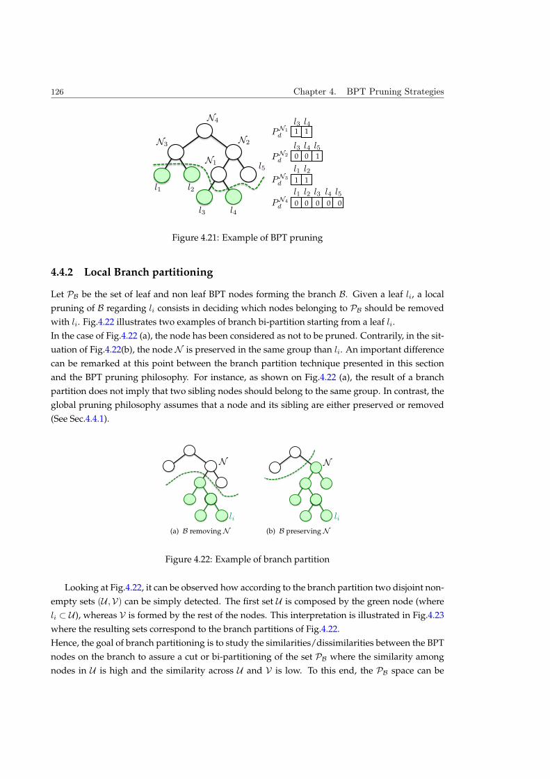
126 Chapter 4. BPT Pruning Strategies
l2
l5N1
l1
l4l3
N2N3
N4
PN1
d
PN2
d
PN3
d
PN4
d
l5l4l3
l4l3
l2l1
l2l1 l3 l4 l5
1 1
100
11
000 0 0
Figure 4.21: Example of BPT pruning
4.4.2 Local Branch partitioning
Let PB be the set of leaf and non leaf BPT nodes forming the branch B. Given a leaf li, a local
pruning of B regarding li consists in deciding which nodes belonging to PB should be removed
with li. Fig.4.22 illustrates two examples of branch bi-partition starting from a leaf li.
In the case of Fig.4.22 (a), the node has been considered as not to be pruned. Contrarily, in the sit-
uation of Fig.4.22(b), the node N is preserved in the same group than li. An important difference
can be remarked at this point between the branch partition technique presented in this section
and the BPT pruning philosophy. For instance, as shown on Fig.4.22 (a), the result of a branch
partition does not imply that two sibling nodes should belong to the same group. In contrast, the
global pruning philosophy assumes that a node and its sibling are either preserved or removed
(See Sec.4.4.1).
(a) B removing N
N
li
(b) B preserving N
N
li
Figure 4.22: Example of branch partition
Looking at Fig.4.22, it can be observed how according to the branch partition two disjoint non-
empty sets (U ,V) can be simply detected. The first set U is composed by the green node (where
li U ), whereas V is formed by the rest of the nodes. This interpretation is illustrated in Fig.4.23
where the resulting sets correspond to the branch partitions of Fig.4.22.
Hence, the goal of branch partitioning is to study the similarities/dissimilarities between the BPT
nodes on the branch to assure a cut or bi-partitioning of the set PB where the similarity among
nodes in U is high and the similarity across U and V is low. To this end, the PB space can be
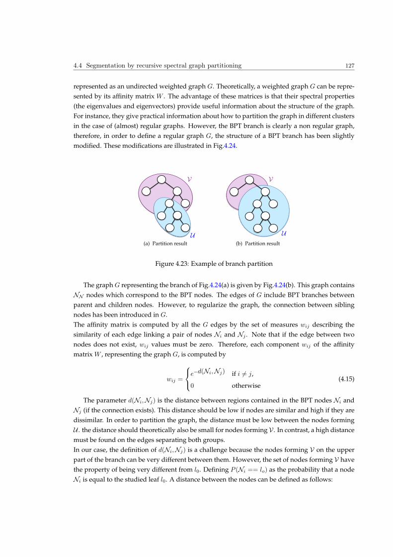
4.4 Segmentation by recursive spectral graph partitioning 127
represented as an undirected weighted graph G. Theoretically, a weighted graph G can be repre-
sented by its affinity matrix W . The advantage of these matrices is that their spectral properties
(the eigenvalues and eigenvectors) provide useful information about the structure of the graph.
For instance, they give practical information about how to partition the graph in different clusters
in the case of (almost) regular graphs. However, the BPT branch is clearly a non regular graph,
therefore, in order to define a regular graph G, the structure of a BPT branch has been slightly
modified. These modifications are illustrated in Fig.4.24.
(a) Partition result
V
U(b) Partition result
V
U
Figure 4.23: Example of branch partition
The graph G representing the branch of Fig.4.24(a) is given by Fig.4.24(b). This graph contains
NN nodes which correspond to the BPT nodes. The edges of G include BPT branches between
parent and children nodes. However, to regularize the graph, the connection between sibling
nodes has been introduced in G.
The affinity matrix is computed by all the G edges by the set of measures wij describing the
similarity of each edge linking a pair of nodes Ni and Nj . Note that if the edge between two
nodes does not exist, wij values must be zero. Therefore, each component wij of the affinity
matrix W , representing the graph G, is computed by
wij =
8
<
:
e−d(Ni,Nj) if i 6= j,
0 otherwise(4.15)
The parameter d(Ni,Nj) is the distance between regions contained in the BPT nodes Ni and
Nj (if the connection exists). This distance should be low if nodes are similar and high if they are
dissimilar. In order to partition the graph, the distance must be low between the nodes forming
U . the distance should theoretically also be small for nodes forming V . In contrast, a high distance
must be found on the edges separating both groups.
In our case, the definition of d(Ni,Nj) is a challenge because the nodes forming V on the upper
part of the branch can be very different between them. However, the set of nodes forming V have
the property of being very different from l0. Defining P (Ni == lo) as the probability that a node
Ni is equal to the studied leaf l0. A distance between the nodes can be defined as follows:
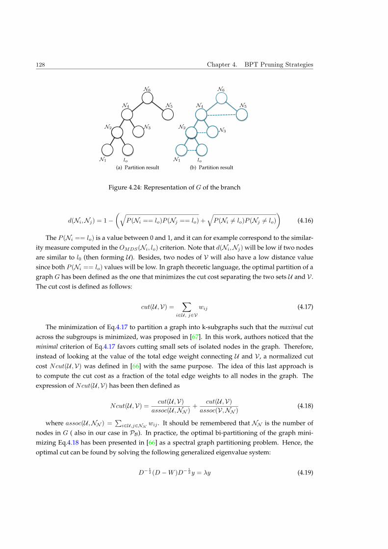
128 Chapter 4. BPT Pruning Strategies
N4 N5
N2 N3
N6
N1 lo
(a) Partition result
N4 N5
N2N3
N6
N1 lo
(b) Partition result
Figure 4.24: Representation of G of the branch
d(Ni,Nj) = 1−
q
P (Ni == lo)P (Nj == lo) +q
P (Ni 6= lo)P (Nj 6= lo)
(4.16)
The P (Ni == lo) is a value between 0 and 1, and it can for example correspond to the similar-
ity measure computed in the OMDS(Ni, lo) criterion. Note that d(Ni,Nj) will be low if two nodes
are similar to l0 (then forming U ). Besides, two nodes of V will also have a low distance value
since both P (Ni == lo) values will be low. In graph theoretic language, the optimal partition of a
graph G has been defined as the one that minimizes the cut cost separating the two sets U and V .
The cut cost is defined as follows:
cut(U ,V) =X
i2U, j2V
wij (4.17)
The minimization of Eq.4.17 to partition a graph into k-subgraphs such that the maximal cut
across the subgroups is minimized, was proposed in [67]. In this work, authors noticed that the
minimal criterion of Eq.4.17 favors cutting small sets of isolated nodes in the graph. Therefore,
instead of looking at the value of the total edge weight connecting U and V , a normalized cut
cost Ncut(U ,V) was defined in [66] with the same purpose. The idea of this last approach is
to compute the cut cost as a fraction of the total edge weights to all nodes in the graph. The
expression of Ncut(U ,V) has been then defined as
Ncut(U ,V) =cut(U ,V)
assoc(U ,NN )+
cut(U ,V)
assoc(V,NN )(4.18)
where assoc(U ,NN ) =P
i2U,j2NNwij . It should be remembered that NN is the number of
nodes in G ( also in our case in PB). In practice, the optimal bi-partitioning of the graph mini-
mizing Eq.4.18 has been presented in [66] as a spectral graph partitioning problem. Hence, the
optimal cut can be found by solving the following generalized eigenvalue system:
D− 12 (D −W )D− 1
2 y = λy (4.19)
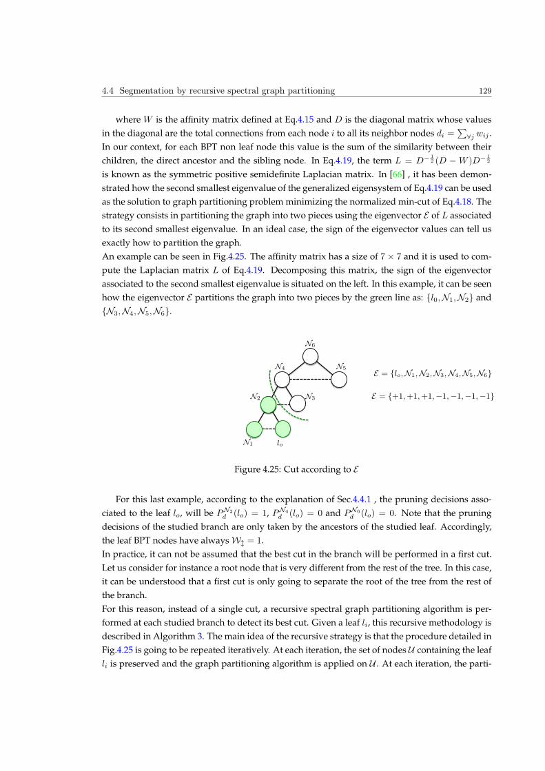
4.4 Segmentation by recursive spectral graph partitioning 129
where W is the affinity matrix defined at Eq.4.15 and D is the diagonal matrix whose values
in the diagonal are the total connections from each node i to all its neighbor nodes di =P
8j wij .
In our context, for each BPT non leaf node this value is the sum of the similarity between their
children, the direct ancestor and the sibling node. In Eq.4.19, the term L = D− 12 (D − W )D− 1
2
is known as the symmetric positive semidefinite Laplacian matrix. In [66] , it has been demon-
strated how the second smallest eigenvalue of the generalized eigensystem of Eq.4.19 can be used
as the solution to graph partitioning problem minimizing the normalized min-cut of Eq.4.18. The
strategy consists in partitioning the graph into two pieces using the eigenvector E of L associated
to its second smallest eigenvalue. In an ideal case, the sign of the eigenvector values can tell us
exactly how to partition the graph.
An example can be seen in Fig.4.25. The affinity matrix has a size of 7 7 and it is used to com-
pute the Laplacian matrix L of Eq.4.19. Decomposing this matrix, the sign of the eigenvector
associated to the second smallest eigenvalue is situated on the left. In this example, it can be seen
how the eigenvector E partitions the graph into two pieces by the green line as: l0,N1,N2 and
N3,N4,N5,N6.
N4 N5
N2 N3
N6
N1 lo
E = lo,N1,N2,N3,N4,N5,N6
E = +1,+1,+1,−1,−1,−1,−1
Figure 4.25: Cut according to E
For this last example, according to the explanation of Sec.4.4.1 , the pruning decisions asso-
ciated to the leaf lo, will be PN2
d (lo) = 1, PN4
d (lo) = 0 and PN6
d (lo) = 0. Note that the pruning
decisions of the studied branch are only taken by the ancestors of the studied leaf. Accordingly,
the leaf BPT nodes have always Wl = 1.
In practice, it can not be assumed that the best cut in the branch will be performed in a first cut.
Let us consider for instance a root node that is very different from the rest of the tree. In this case,
it can be understood that a first cut is only going to separate the root of the tree from the rest of
the branch.
For this reason, instead of a single cut, a recursive spectral graph partitioning algorithm is per-
formed at each studied branch to detect its best cut. Given a leaf li, this recursive methodology is
described in Algorithm 3. The main idea of the recursive strategy is that the procedure detailed in
Fig.4.25 is going to be repeated iteratively. At each iteration, the set of nodes U containing the leaf
li is preserved and the graph partitioning algorithm is applied on U . At each iteration, the parti-
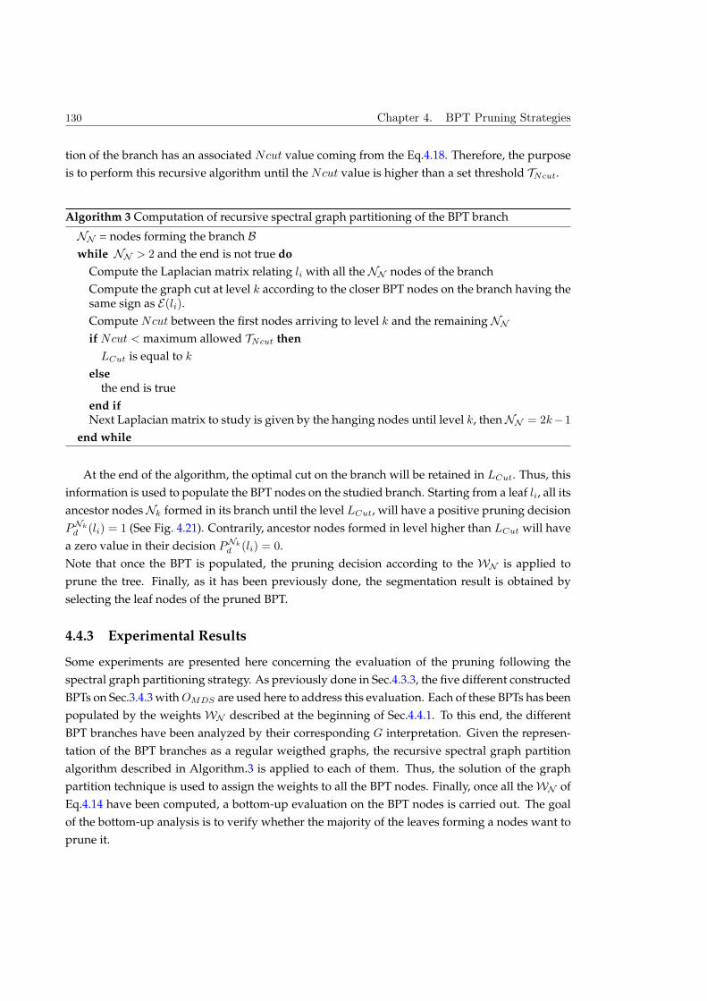
130 Chapter 4. BPT Pruning Strategies
tion of the branch has an associated Ncut value coming from the Eq.4.18. Therefore, the purpose
is to perform this recursive algorithm until the Ncut value is higher than a set threshold TNcut.
Algorithm 3 Computation of recursive spectral graph partitioning of the BPT branch
NN = nodes forming the branch B
while NN > 2 and the end is not true do
Compute the Laplacian matrix relating li with all the NN nodes of the branch
Compute the graph cut at level k according to the closer BPT nodes on the branch having thesame sign as E(li).
Compute Ncut between the first nodes arriving to level k and the remaining NN
if Ncut < maximum allowed TNcut then
LCut is equal to k
elsethe end is true
end ifNext Laplacian matrix to study is given by the hanging nodes until level k, then NN = 2k−1
end while
At the end of the algorithm, the optimal cut on the branch will be retained in LCut. Thus, this
information is used to populate the BPT nodes on the studied branch. Starting from a leaf li, all its
ancestor nodes Nk formed in its branch until the level LCut, will have a positive pruning decision
PNk
d (li) = 1 (See Fig. 4.21). Contrarily, ancestor nodes formed in level higher than LCut will have
a zero value in their decision PNk
d (li) = 0.
Note that once the BPT is populated, the pruning decision according to the WN is applied to
prune the tree. Finally, as it has been previously done, the segmentation result is obtained by
selecting the leaf nodes of the pruned BPT.
4.4.3 Experimental Results
Some experiments are presented here concerning the evaluation of the pruning following the
spectral graph partitioning strategy. As previously done in Sec.4.3.3, the five different constructed
BPTs on Sec.3.4.3 with OMDS are used here to address this evaluation. Each of these BPTs has been
populated by the weights WN described at the beginning of Sec.4.4.1. To this end, the different
BPT branches have been analyzed by their corresponding G interpretation. Given the represen-
tation of the BPT branches as a regular weigthed graphs, the recursive spectral graph partition
algorithm described in Algorithm.3 is applied to each of them. Thus, the solution of the graph
partition technique is used to assign the weights to all the BPT nodes. Finally, once all the WN of
Eq.4.14 have been computed, a bottom-up evaluation on the BPT nodes is carried out. The goal
of the bottom-up analysis is to verify whether the majority of the leaves forming a nodes want to
prune it.
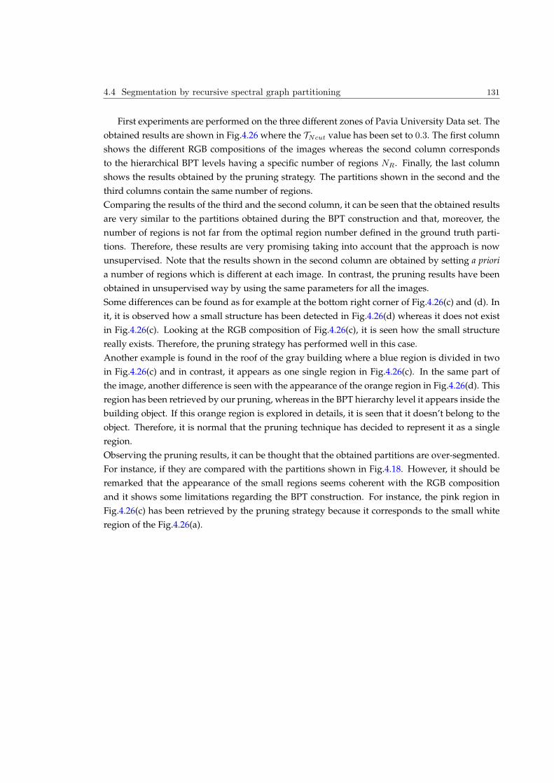
4.4 Segmentation by recursive spectral graph partitioning 131
First experiments are performed on the three different zones of Pavia University Data set. The
obtained results are shown in Fig.4.26 where the TNcut value has been set to 0.3. The first column
shows the different RGB compositions of the images whereas the second column corresponds
to the hierarchical BPT levels having a specific number of regions NR. Finally, the last column
shows the results obtained by the pruning strategy. The partitions shown in the second and the
third columns contain the same number of regions.
Comparing the results of the third and the second column, it can be seen that the obtained results
are very similar to the partitions obtained during the BPT construction and that, moreover, the
number of regions is not far from the optimal region number defined in the ground truth parti-
tions. Therefore, these results are very promising taking into account that the approach is now
unsupervised. Note that the results shown in the second column are obtained by setting a priori
a number of regions which is different at each image. In contrast, the pruning results have been
obtained in unsupervised way by using the same parameters for all the images.
Some differences can be found as for example at the bottom right corner of Fig.4.26(c) and (d). In
it, it is observed how a small structure has been detected in Fig.4.26(d) whereas it does not exist
in Fig.4.26(c). Looking at the RGB composition of Fig.4.26(c), it is seen how the small structure
really exists. Therefore, the pruning strategy has performed well in this case.
Another example is found in the roof of the gray building where a blue region is divided in two
in Fig.4.26(c) and in contrast, it appears as one single region in Fig.4.26(c). In the same part of
the image, another difference is seen with the appearance of the orange region in Fig.4.26(d). This
region has been retrieved by our pruning, whereas in the BPT hierarchy level it appears inside the
building object. If this orange region is explored in details, it is seen that it doesn’t belong to the
object. Therefore, it is normal that the pruning technique has decided to represent it as a single
region.
Observing the pruning results, it can be thought that the obtained partitions are over-segmented.
For instance, if they are compared with the partitions shown in Fig.4.18. However, it should be
remarked that the appearance of the small regions seems coherent with the RGB composition
and it shows some limitations regarding the BPT construction. For instance, the pink region in
Fig.4.26(c) has been retrieved by the pruning strategy because it corresponds to the small white
region of the Fig.4.26(a).

132 Chapter 4. BPT Pruning Strategies
(a) RGB (b) NR = 29 (c) NR = 29
(d) RGB (e) NR = 22 (f) NR = 22
(g) RGB (h) NR = 34 (i) NR = 34
Figure 4.26: Comparison of Hierarchical BPT level(center) and pruned BPT(right) partitions
A second set of experiments is carried out on the Pavia Center and Hydice images. For both
images, the same pruning strategy is carried out leading to the results of Fig.4.27. In the case of
Pavia Center, the pruning results clearly outperform the hierarchical level since the background
is only formed by a single region. An interesting phenomenon is observed in Fig.4.27(c) where
4 regions on the left part of the image have been detected individually. In all the other results
obtained during this PhD on this data set, these four regions appear as a single purple region.
However, looking at the RGB composition of Fig.4.27, it can be corroborated how this part of the
image is formed by more than one region.
Concerning HYDICE results, both images present very similar results. A small difference can be
seen as for example on the top right part of the image. The pruning results show an orange region
separated from the road whereas the same region has been merged with the road in Fig.4.27(e).
Looking at the RGB composition Fig.4.27(d), it seems that the pruning result is the wrong one.
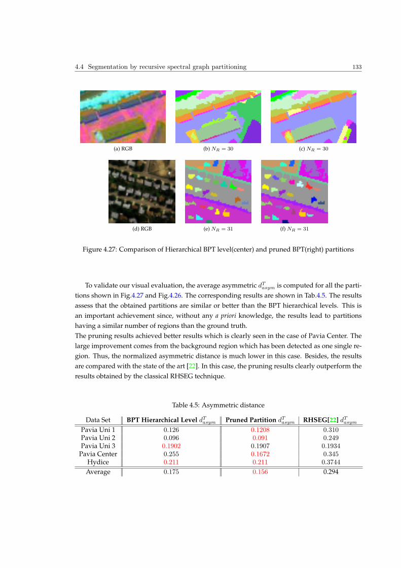
4.4 Segmentation by recursive spectral graph partitioning 133
(a) RGB (b) NR = 30 (c) NR = 30
(d) RGB (e) NR = 31 (f) NR = 31
Figure 4.27: Comparison of Hierarchical BPT level(center) and pruned BPT(right) partitions
To validate our visual evaluation, the average asymmetric dTasym is computed for all the parti-
tions shown in Fig.4.27 and Fig.4.26. The corresponding results are shown in Tab.4.5. The results
assess that the obtained partitions are similar or better than the BPT hierarchical levels. This is
an important achievement since, without any a priori knowledge, the results lead to partitions
having a similar number of regions than the ground truth.
The pruning results achieved better results which is clearly seen in the case of Pavia Center. The
large improvement comes from the background region which has been detected as one single re-
gion. Thus, the normalized asymmetric distance is much lower in this case. Besides, the results
are compared with the state of the art [22]. In this case, the pruning results clearly outperform the
results obtained by the classical RHSEG technique.
Table 4.5: Asymmetric distance
Data Set BPT Hierarchical Level dTasym Pruned Partition dTasym RHSEG[22] dTasymPavia Uni 1 0.126 0.1208 0.310Pavia Uni 2 0.096 0.091 0.249Pavia Uni 3 0.1902 0.1907 0.1934
Pavia Center 0.255 0.1672 0.345Hydice 0.211 0.211 0.3744
Average 0.175 0.156 0.294
134 Chapter 4. BPT Pruning Strategies
Conclusions
In an unsupervised segmentation framework, the BPT pruning has been considered here as a
graph cut problem. The study of the BPT branches to decide the best branch cut has been carried
out by a classical technique proposed in [66]. The proposed approach has allowed to compute the
affinity matrices describing the image relations by using different regions of an image. This in-
troduces a novelty regarding the state of the art where the graph cut techniques is applied on the
RAG pixel representation. Hence, classical works have computed the affinity matrix representing
a region simply by studying the pixel similarities. Here, the construction of the affinity matrices
using regions has been proposed. In this work, a similarity function relying on the spectrum in-
formation has been applied to weight the edges of the graph. However, note that having regions,
the affinity matrix could use more information as such the shape of regions.
Looking at all the obtained results, it can be observed how the pruning strategy has lead to in-
teresting results. The obtained partitions are coherent with the realistic RGB composition. The
asymmetric distance computed on the different results has shown the improvement achieved by
the BPT pruning strategy. Indeed, the obtained partitions have been obtained without any priori
knowledge (such as a given number of regions). Comparing our asymmetric distance results with
the results obtained in Sec.3.4.3 , it can be noticed that the pruning strategy has achieved parti-
tions situated close to the minimum of the dasym curves.
In this section as well as in Sec.4.3, it has been seen that because of the complexity of the scenes,
it is sometimes difficult to define the ground truth partitions. A detailed analysis of the results
reveals that some of the observed differences are subject to interpretation. On the other hand, the
results have also shown that some mistakes were generated during the BPT construction. As the
pruning results directly depend on the BPT construction, if a region is not perfectly represented
by BPT nodes, the pruning strategy cannot retrieve it.
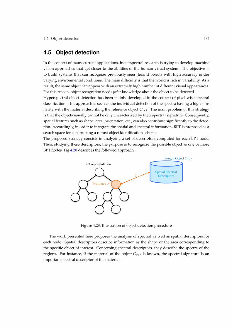
4.5 Object detection 135
4.5 Object detection
In the context of many current applications, hyperspectral research is trying to develop machine
vision approaches that get closer to the abilities of the human visual system. The objective is
to build systems that can recognize previously seen (learnt) objects with high accuracy under
varying environmental conditions. The main difficulty is that the world is rich in variability. As a
result, the same object can appear with an extremely high number of different visual appearances.
For this reason, object recognition needs prior knowledge about the object to be detected.
Hyperspectral object detection has been mainly developed in the context of pixel-wise spectral
classification. This approach is seen as the individual detection of the spectra having a high sim-
ilarity with the material describing the reference object Oref . The main problem of this strategy
is that the objects usually cannot be only characterized by their spectral signature. Consequently,
spatial features such as shape, area, orientation, etc., can also contribute significantly to the detec-
tion. Accordingly, in order to integrate the spatial and spectral information, BPT is proposed as a
search space for constructing a robust object identification scheme.
The proposed strategy consists in analyzing a set of descriptors computed for each BPT node.
Thus, studying these descriptors, the purpose is to recognize the possible object as one or more
BPT nodes. Fig.4.28 describes the followed approach.
Sought Object Oref
Spatial-SpectralDescriptors?
BPT representation
Evaluated N
Figure 4.28: Illustration of object detection procedure
The work presented here proposes the analysis of spectral as well as spatial descriptors for
each node. Spatial descriptors describe information as the shape or the area corresponding to
the specific object of interest. Concerning spectral descriptors, they describe the spectra of the
regions. For instance, if the material of the object Oref is known, the spectral signature is an
important spectral descriptor of the material.
136 Chapter 4. BPT Pruning Strategies
Accordingly, the proposed scheme relies on the three different descriptors for the BPT nodes
O = Dshape, Dspectral, Darea (4.20)
The computation of the set of descriptors for the nodes populates the BPT in this application.
Thus, once the proposed descriptors D are computed, they are studied from the leaves to the root.
The approach consists in removing all nodes that significantly differ from the characterization
proposed by the reference Oref . Hence, the idea consists in considering that the sought objects
are defined by the closest nodes to the root node that have a set descriptors close to the Oref
model. In order to illustrate the generality of the approach, two detection examples are presented
here: road and building detection in urban scenes, respectively.
4.5.1 Detection of roads
Roads appear as elongated structures having fairly homogeneous radiance values usually cor-
responding to asphalt. In a classical pixel-wise classification, the detection of the roads clearly
consists in detecting the possible pixels of the image that belong to the asphalt class. The main
drawback is that other structures of the image can also be formed by asphalt. To solve this issue,
an information is that roads appear as stretched objects. Thus, given their characteristic shape, the
region elongation is used here as the shape descriptor Dshape. In order to compute it, the smallest
oriented rectangular bounding box must be computed for each region contained in a BPT node.
The oriented bounding box of the region containing N is the smallest rectangle including the region
that is aligned with its orientation φ. Knowing this value, the rotation of coordinates x, y is given
by
↵ = xcosφ+ ysinφ (4.21)
β = xsinφ+ ycosφ (4.22)
The last transformation defines new coordinates ↵ and β which are used to describe the points
P1, P2, P3 and P4 characterizing the oriented bounding box (See Fig.4.29). Once the oriented
bounding box of a region is computed, the elongation of the region, corresponding to the Dshape,
can be easily computed as the ratio between the width and the height of the bounding box.
The second spatial descriptor computed at BPT nodes is the area of the region Darea. The idea is
that a road should have at least a given number of pixels. This minimum required area should be
set according to the spatial resolution of the image.
Concerning the spectral descriptor Dspectral, it must contained the information concerning whether
the region on the BPT node is formed by asphalt. Thus, given a reference spectrum of the road
material, the correlation coefficient between the mean spectrum of the BPT node and a reference
spectrum of the road material is used as Dspectral. This coefficient can be computed by Eq.4.23
where INλ is the average spectrum contained in N .
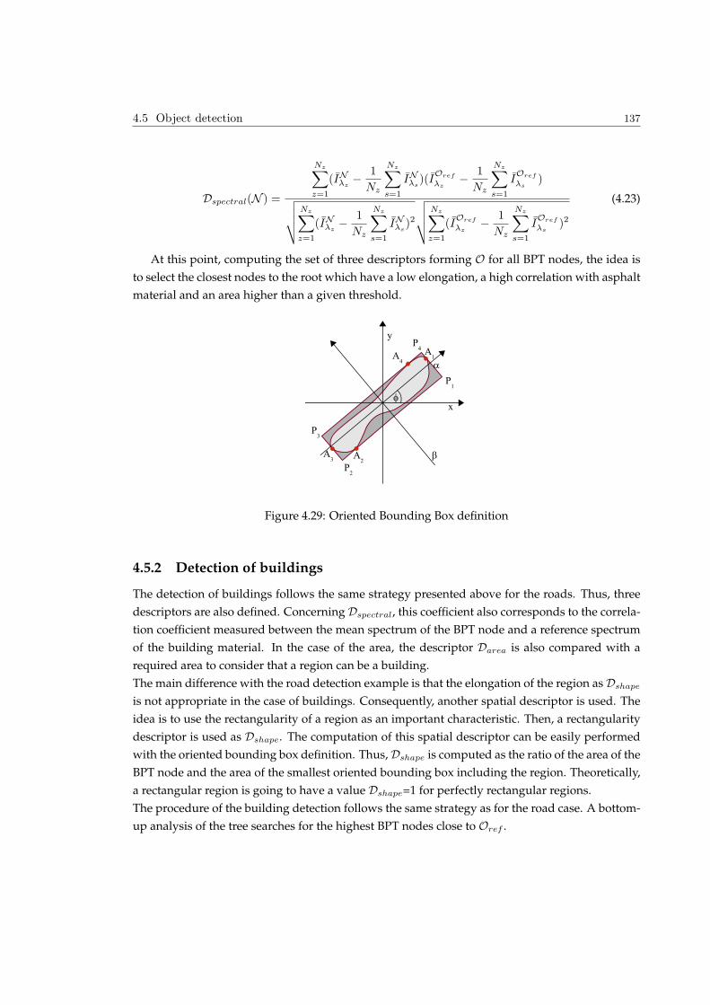
4.5 Object detection 137
Dspectral(N ) =
NzX
z=1
(INλz−
1
Nz
NzX
s=1
INλs)(I
Oref
λz−
1
Nz
NzX
s=1
IOref
λs)
vuut
NzX
z=1
(INλz−
1
Nz
NzX
s=1
INλs)2
vuut
NzX
z=1
(IOref
λz−
1
Nz
NzX
s=1
IOref
λs)2
(4.23)
At this point, computing the set of three descriptors forming O for all BPT nodes, the idea is
to select the closest nodes to the root which have a low elongation, a high correlation with asphalt
material and an area higher than a given threshold.
Figure 4.29: Oriented Bounding Box definition
4.5.2 Detection of buildings
The detection of buildings follows the same strategy presented above for the roads. Thus, three
descriptors are also defined. Concerning Dspectral, this coefficient also corresponds to the correla-
tion coefficient measured between the mean spectrum of the BPT node and a reference spectrum
of the building material. In the case of the area, the descriptor Darea is also compared with a
required area to consider that a region can be a building.
The main difference with the road detection example is that the elongation of the region as Dshape
is not appropriate in the case of buildings. Consequently, another spatial descriptor is used. The
idea is to use the rectangularity of a region as an important characteristic. Then, a rectangularity
descriptor is used as Dshape. The computation of this spatial descriptor can be easily performed
with the oriented bounding box definition. Thus, Dshape is computed as the ratio of the area of the
BPT node and the area of the smallest oriented bounding box including the region. Theoretically,
a rectangular region is going to have a value Dshape=1 for perfectly rectangular regions.
The procedure of the building detection follows the same strategy as for the road case. A bottom-
up analysis of the tree searches for the highest BPT nodes close to Oref .

138 Chapter 4. BPT Pruning Strategies
4.5.3 Experimental Results
This section addresses the evaluation of the BPT object detection strategy proposed for the road
and building detection. The goal of the experiments is to compare the results of the BPT object
recognition strategy with a classical unsupervised pixel-wise classification. The experiments have
been performed using the portion of HYDICE hyperspectral image of Sec.3.4.2. Fig. 4.30(a) shows
a RGB combination of the image portion. The BPT has been computed with the OMDS . The
ground truth partition of this image illustrating the roads and buildings of the scene are shown
in Fig. 4.30(b) and Fig. 4.30(c).
(a) RGB Composition (b) Roads PGT (c) Buildings PGT
Figure 4.30: Hydice Data Set
The pixel-wise classification consists in detecting pixels in the image having a correlation
higher than 0.9 with the reference spectrum.
To detect Oref some reference parameters should be set. For instance, in the case of roads, the
pruning strategy is looking for regions having an elongation lower than 0.3, with a correlation co-
efficient with asphalt higher than 0.9 and an area larger than 15 pixels. Regarding the buildings,
the BPT analysis is focused on detecting regions having a rectangularity higher than 0.4, a corre-
lation coefficient between building material higher than 0.9 and an area smaller than 15 pixels.
The first row of Fig. 4.31 shows the results of the pixel-wise classification road and building hav-
ing a high correlation coefficient. The second row of Fig. 4.31 illustrates the detected BPT nodes
using the two different Dref . The results obtained with the BPT corroborate the advantage of
using this image representation. The use of spectral as well as spatial descriptors of BPT nodes
outperforms the classical pixel-wise detection using only spectral information.
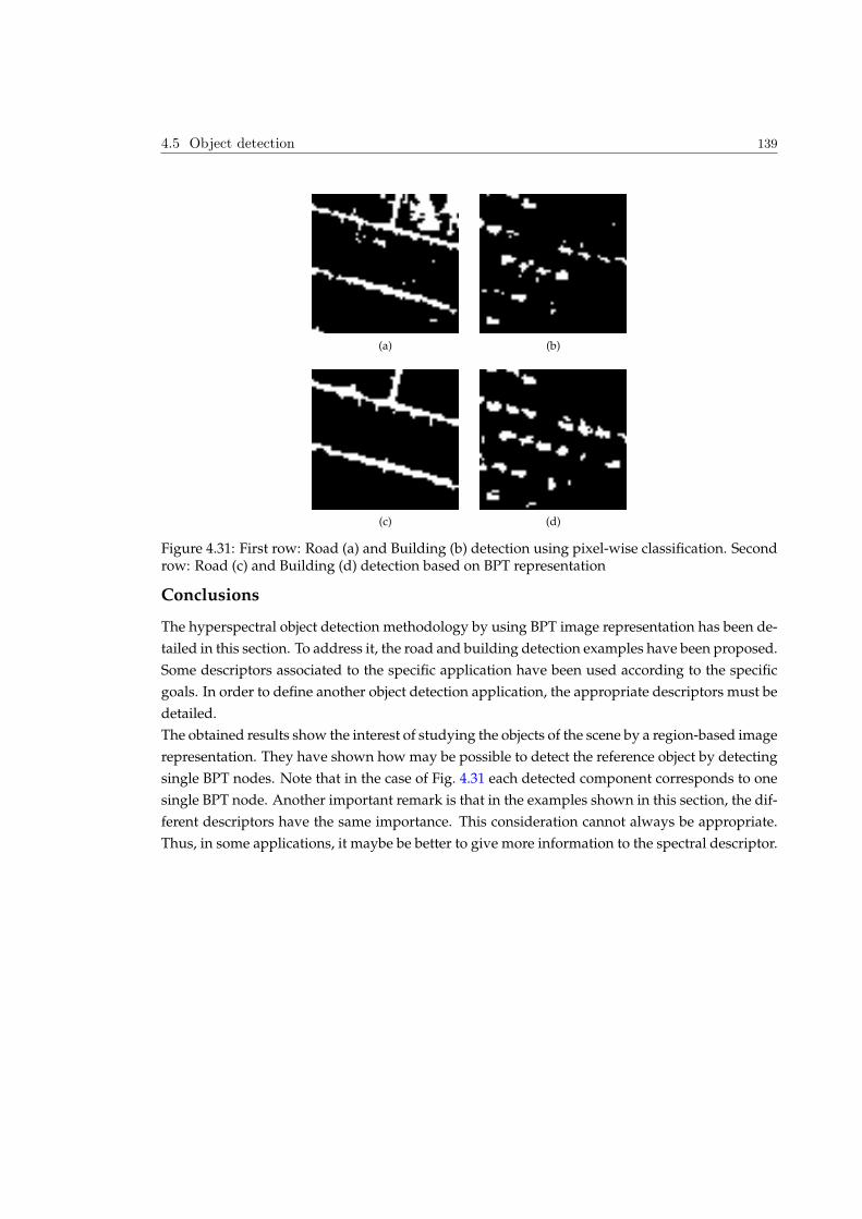
4.5 Object detection 139
(a) (b)
(c) (d)
Figure 4.31: First row: Road (a) and Building (b) detection using pixel-wise classification. Secondrow: Road (c) and Building (d) detection based on BPT representation
Conclusions
The hyperspectral object detection methodology by using BPT image representation has been de-
tailed in this section. To address it, the road and building detection examples have been proposed.
Some descriptors associated to the specific application have been used according to the specific
goals. In order to define another object detection application, the appropriate descriptors must be
detailed.
The obtained results show the interest of studying the objects of the scene by a region-based image
representation. They have shown how may be possible to detect the reference object by detecting
single BPT nodes. Note that in the case of Fig. 4.31 each detected component corresponds to one
single BPT node. Another important remark is that in the examples shown in this section, the dif-
ferent descriptors have the same importance. This consideration cannot always be appropriate.
Thus, in some applications, it maybe be better to give more information to the spectral descriptor.
140 Chapter 4. BPT Pruning Strategies
4.6 Conclusions
This chapter has discussed different BPT processing techniques. The main purpose has been to
demonstrate how different pruning strategies can be defined on the BPT structure according to
specific applications. Three different applications have been studied in order to prune the tree.
Firstly, a supervised hyperspectral image classification has been proposed using the SVM clas-
sifier. Then, the hyperspectral image segmentation challenge has been studied by a supervised
and an unsupervised pruning strategy. Finally, the hyperspectral object detection using the BPT
image representation has been explained with two different examples.
In each case, the processing of the BPT has been done in two steps. Firstly, BPT nodes are popu-
lated by computing some descriptors or features. Secondly, the analysis of the node descriptors
along the BPT branches decides whether nodes should be removed or preserved.
Concerning the first step, different descriptors have been presented according to the applications.
For instance, in the classification case, a descriptor related to the misclassification rate has been
proposed. The goal of this descriptor is the evaluation of the error committed by removing nodes
having a class different from their direct descendants. The computation of this rate has been
performed by using the SVM supervised classifier. In the case of segmentation, two different ap-
proaches have been discussed. In the first approach, a supervised pruning based on an energy
minimization strategy has been presented. In this context, BPT nodes have been populated by
a spectral homogeneity descriptor. In this case, the idea has been to describe if the regions are
spectrally homogeneous with respect to their mean spectrum. The second approach involving
segmentation has been presented as an unsupervised BPT pruning technique. In this case, the
BPT nodes have been populated by weights representing local pruning decisions. Studying sep-
arately each branch, the proposed methodology analyses if the ancestor nodes can replace their
leaves. Finally, in the case of object detection, nodes have been populated with spatial and spec-
tral descriptors. The descriptor choice is directly related with the road and building detection
application. The elongation and the rectangularity of the regions have been proposed as spatial
descriptors. Regarding the spectral descriptor, the correlation coefficient with the reference mate-
rial has been used.
Once the BPT nodes have been populated, different strategies have been proposed in order to
decide the pruning of the nodes. In all cases, a bottom-up analysis of the tree from the leaves to
the root has been performed. Therefore, some pruning rules have been defined for the different
BPT pruning strategies. In the first pruning strategy involving the hyperspectral image classifi-
cation, the maximum decision rule has been used. In this context, the classification results have
shown the benefit of using the BPT image representation. Classification accuracies have clearly
outperformed the classical results obtained by the standard pixel-wise classification. Besides the
quantitative results, the obtained classification maps have shown homogeneous regions without
involving the classical impulsive classification noise.

4.6 Conclusions 141
For segmentation, a supervised pruning technique performing a global analysis has been pro-
posed. This technique has been presented as an energy minimization problem subject to a con-
straint. The constraint corresponds to the desired number of regions. Note that because of this
constraint this pruning is supervised. In this case, promising results have been obtained. How-
ever, the main drawback of this technique is that the number of regions forming the partition
should be known a priori. Hence, this approach does not seem to be appropriate for most prac-
tical solutions. Therefore, an unsupervised pruning strategy has been proposed based on the
spectral graph partitioning theory.
This last pruning technique have provided the best performances. The partition results have been
compared with the partitions obtained during the merging sequence construction and with the
state of the art. The quantitative evaluations have corroborated the robustness of the pruning.
In the case of object detection, two different pruning examples have been presented for two object
detection examples. Setting the detection of roads and building as main goals, very interesting
and promising results have been obtained.
The four pruning strategies have shown how the BPT representation can be used in different con-
texts. Moreover, the obtained results have corroborated the interest of studying hyperspectral
images by using a region-based representation like the BPT.

142 Chapter 4. BPT Pruning Strategies
5Conclusions
In this thesis, the BPT region-based representation for hyperspectral imagery has been presented
as a very promising area of research [70]. The construction and the processing of the BPT rep-
resentation in a hyperspectral context have been discussed. This tree-based structure has been
preferred in to other graph structures since BPT succeeds in representing : 1) the decomposition
of the image in terms of regions representing objects and 2) the inclusion relations of the regions
in the scene. Furthermore, given its fixed structure, BPT allows implementing efficient and ad-
vanced application-dependent techniques on it. In this framework, the work addressed in this
thesis is mainly divided in two parts: the BPT construction and the BPT processing.
The BPT construction for hyperspectral imaging has been investigated in Chapter 3. Conse-
quently, the first main challenge in this Phd has been the definition of a region merging algo-
rithm. This task has not been straightforward. This has been explained by the complexity of the
data given the variability of the spectra and the high correlation between bands. To address these
issues, several regions models and merging criteria have been studied [69]. Concerning the region
models, the popular region model described here as the first-order model has been compared with
the non parametric statistical region model previously defined in [17] for classical imagery. The
use of non parametric statistical region model has been proposed as a solution for representing
a set of spectra. This region model has shown its performances to solve the spectral variability
issue. Furthermore, it has proved its capabilities to represent complex or textured regions. In
order to compute this model for the individual spectra of the image, robust algorithm to estimate
the pdf of initial pixels based on self-similarity ideas has been proposed in Sec.3.2.2. To be able to
144 Chapter 5. Conclusions
estimate the pdf of individual spectra, a noise estimation in the case of the hyperspectral image
bands has been detailed in the same section. This noise estimation can be used in future works to
define a noise reduction strategy in hyperspectral image based on a non-local mean procedure.
According to the non parametric statistical region model, different merging criteria have been
proposed. The problem associated to the Battacharyya distance described in [17] has been solved
by using the cross-bin Diffusion distance. The use of a cross-bin distance has corroborated its ad-
vantage showing in particular its robustness to the Nbins parameter. Although this distance may
be less accurate than other cross-bin histogram distances known in the literature such as Earth
Mover Distance L1, it has been chosen because of its trade-off between complexity and accuracy.
Despite of the interesting results provided by the metrics comparing histograms, the correlation
issue was not addressed in this case.
Hence, a new merging criterion taking into account the correlation between hyperspectral bands
has been proposed as one of the main contributions of the PhD in Sec.3.3.3. The idea has been
to locally reduce the dimension of the region model via multidimensional scaling. Studying the
similarities between the histograms of the region, the local principal coordinates of each region
has been extracted. Then, a statistical test based on MANOVA theory has been proposed to mea-
sure the similarity between two adjacent regions. This test has also been directly related with the
canonical correlations. In this context, an estimation of the best dimension to compare the princi-
pal coordinates of two regions has been presented in this work. In order to compare two principal
components data sets representing two hyperspectral regions, a trade-off between the principal
coordinates of each data set has been proposed.
To compare the different merging orders, an evaluation has been carried out by evaluating the
partitions obtained during the merging sequence construction. In order to evaluate the results,
a visual and a quantitative evaluation have been carried out. The quantitative assessment has
been performed wiht the symmetric and the asymmetric distances presented in Sec.3.4.1. To our
knowledge, this Phd has introduced the first quantitative evaluation to validate the hyperspec-
tral image partitions concerning the whole image. Experimental results have shown the good
performances of the BPT construction in comparison with the most used state of the art tech-
nique: RHSEG [22]. The obtained results have also shown the limitations of the first order region
model. In contrast, the merging criterion via MDS has obtained the best results in our study. Thus,
this merging criterion can be considered as a promising measure to establish similarities between
spectral data sets in future works.
The second main important contribution shown in this thesis is the different BPT processing tech-
niques which have been targeted for different applications. Four different strategies have been
presented in the context of supervised hyperspectral image classification, supervised and unsu-
pervised hyperspectral image segmentation and finally, object detection. The processing of BPT
has been presented in Chapter 4 as a pruning strategy based on performing an analysis of the
nodes of the tree by measuring a specific criterion . The different strategies have corroborated
how the BPT is not an application-dependent tree structure, but it is an image representation
which can be processed by several application-dependent strategies.
145
As a first example of pruning, the supervised classification of hyperspectral image has been ad-
dressed. The SVM classifier has been used to populate the BPT nodes with the probability class
distribution. Then, a bottom-up analysis of the tree branches has removed the BPT nodes fol-
lowing a maximum rule decision. Experimental results have shown that the proposed method
improves the classification accuracies of a standard SVM, providing classification maps with a
reduced amount of noise.
The second pruning strategy was targeting a supervised segmentation. This pruning technique
has been presented as a global energy minimization problem on the BPT structure. Under this
framework, a constrained Lagrangian function has been proposed by using a spectral homogene-
ity descriptor. The constraint parameter has been set as the desired number of regions. The main
goal of this pruning has been to show that if the desired number of regions is known, the partition
involving this number of regions obtained following the merging sequence construction is not op-
timal. In other words, the pruning technique aims at extracting the same number of regions but
with higher homogeneity. Experiments have been conduced to compare the partitions obtained
from the merging sequence with those obtained through the pruning. The pruning results have
shown some improvements in their accuracies. However, it must be remarked that the OMDS
criterion has constructed a quite good BPT representation, therefore, to achieve a large improve-
ment is a challenging task. The formulation of the BPT pruning as global minimization problem
offers a very promising line of work for the future leading to robust strategies.
Nevertheless, supervised segmentation cannot be widely used in practice. Indeed, the number
of regions is most of the time unknown and moreover, it is strongly image-dependant. Hence,
in order to tackle this problem, the segmentation of hyperspectral images with an unsupervised
pruning strategy has been studied. To this end, a pruning strategy based on normalized cut has
been proposed.
The analysis of BPT branches to decide the best cut has been addressed by interpreting the BPT
branches as regular graphs by including the sibling node connections. Then, the spectral graph
partitioning theory has been applied to obtain normalized cut. The aim of the cut has been to par-
tition the branch in two disjoint data sets. As a result, the cut on the branch must be considered as
a local pruning . Therefore, the solution of the branch cut has been used here to populate the BPT
nodes using weights describing how likely is the pruning of a node. These weights have been
used later to perform a bottom-up analysis of the tree according to a maximum decision rule. This
rule has been defined as a majority vote comparing the weight of a node with its area.
The results obtained by this pruning are very positive since using the same parameters, it has
been possible to extract partitions with similar number of regions as the ground truth partitions
and with the highest quality compared to the remaining segmentation strategies discussed in this
PhD. The results have shown how a hyperspectral image is partitioned in coherent regions com-
pared to the ground truth. One of the possible limitations of this pruning is that the study of
the branches is done locally. Thus, the application of the spectral graph theory to the complete
tree structure could be envisaged as future research work. Futhermore, the computation of the
affinity matrices by using BPT image representation seems to be an encouraging line of research.

146 Chapter 5. Conclusions
Indeed, the computation of this matrices has been mainly done in the literature for classical RAG
structures. Therefore, the idea of using a hierarchical image representation could lead to better
results.
The last pruning example has been presented in the framework of object detection. Two examples
have been proposed in order to illustrate how BPT can be a powerful representation for the object
recognition applications. To this end, the road and the building examples have been shown. Such
examples have described how the spectral and the spatial information can be incorporated in the
search of a reference object. This work can be seen as a contribution in the hyperspectral field.
Indeed, in most of the work reported in the literature, object detection has been only based on a
pixel-wise classification algorithm by selecting pixels spectrally similar to a pre-defined class.

6Appendix
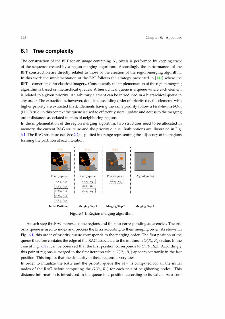
148 Chapter 6. Appendix
6.1 Tree complexity
The construction of the BPT for an image containing Np pixels is performed by keeping track
of the sequence created by a region-merging algorithm. Accordingly the performances of the
BPT construction are directly related to those of the creation of the region-merging algorithm.
In this work the implementation of the BPT follows the strategy presented in [141] where the
BPT is constructed for classical imagery. Consequently the implementation of the region merging
algorithm is based on hierarchical queues. A hierarchical queue is a queue where each element
is related to a given priority. An arbitrary element can be introduced in a hierarchical queue in
any order. The extraction is, however, done in descending order of priority (i.e. the elements with
higher priority are extracted first). Elements having the same priority follow a First-In-First-Out
(FIFO) rule. In this context the queue is used to efficiently store, update and access to the merging
order distances associated to pairs of neighboring regions.
In the implementation of the region merging algorithm, two structures need to be allocated in
memory, the current RAG structure and the priority queue. Both notions are illustrated in Fig.
6.1. The RAG structure (see Sec.2.2) is plotted in orange representing the adjacency of the regions
forming the partition at each iteration.
Priority queue
O(R3, R4) O(R1, R2)
O(R2, R5)
O(R1, R5)
O(R5, R6)
O(R1, R2)
O(R4, R2)
O(R1, R4)
O(R1, R3)
RAG
R1
R3
R4
R2
Priority queue
RAG
R1
R2
R5
Priority queue
RAG
R6
R5
Algorithm End
R7
Initial Partition Merging Step 1 Merging Step 2 Merging Step 3
Figure 6.1: Region merging algorithm
At each step the RAG represents the regions and the four corresponding adjacencies. The pri-
ority queue is used to index and process the links according to their merging order. As shown in
Fig. 6.1, this order of priority queue corresponds to the merging order. The first position of the
queue therefore contains the edge of the RAG associated to the minimum O(Ri, Rj) value. In the
case of Fig. 6.1 it can be observed that the first position corresponds to O(R3, R4). Accordingly
this pair of regions is merged in the first iteration while O(R3, R1) appears contrarily in the last
position. This implies that the similarity of these regions is very low.
In order to initialize the RAG and the priority queue the MRiis computed for all the initial
nodes of the RAG before computing the O(Ri, Rj) for each pair of neighboring nodes. This
distance information is introduced in the queue in a position according to its value. As a con-

6.1 Tree complexity 149
sequence, whether the initial partition is made of single-pixel regions and the neighborhood is
four-connected, the queue is initially formed by Np multiplied by the all pair of regions according
to the four-connectivity.
After each merging the queue is updated in two sequential steps, (i) by removing the old links
concerning the merged nodes, and (ii) by updating the new links representing the adjacency of
the new regions with its neighbors. The algorithm used to insert, to delete and to search the nodes
relies on a balanced tree binary search. The number of steps required for searching, inserting and
deleting nodes in the queue can be therefore done in O(log2N) where N is the number of nodes
in the tree [142] [141].
In order to construct the BPT Np − 1 merging iterations are performed after which the queue is
empty. Accordingly the number of operations Ototal required by this implementation is given by
Ototal = Oinitial + (Np − 1) ∗Oupdate (6.1)
where Oinitial is the number of operations at the initialization step and Oupdate is the number
of operations required for updating the new links. The former task consists of two different sub-
tasks as shown in Eq.6.2. First, the Np region models are computed where Oini node represents
the number of operations required by the construction of a BPT leaf. Second, the corresponding
distance Omerging between its four neighboring pixels is computed for each leaf node.
Oinitial = Np ∗Oini node +Np ∗ 4 ∗Omerging (6.2)
The second term of Eq.6.1 corresponds to the Np − 1 iterations that have to be performed.
Note that the term Np ∗ 4 can be lower if a neighboring pixel has been previously initialized. The
term Oupdated is the number of required operations after a region merging step corresponding to
the update of the queue, which are described by Eq.6.3. At each iteration, a new node is formed
and the corresponding region model is computed. The second term of Eq.6.3 corresponds to the
update of distances between the old neighbors of the removed regions and the newly formed
region. It must be noted that the number of distances to be computed at this step depends on a
factor K. This factor corresponds to the number of links to be updated and it depends on the tree
construction (if it is more or less balanced).
Oupdate = Onode +K ∗Omerging (6.3)
This last equation shows the strong dependence of the complexity of the BPT construction on
three factors, (i) the number of pixels of the image Np, (ii) the operations required for the creation
of a node after a merging Onode, and (iii) the complexity of the merging criteria Omerging between
each pair of adjacent regions.
In order to minimize the computational load the previous bottlenecks of the tree must be studied.
As for parameter Np, it is evident that the number of pixels of the image cannot be modified.
However, in order to reduce the computational load in some applications it might be interesting
to start where pixels are not single individual regions as it is done in Fig. 6.1. For instance, an
150 Chapter 6. Appendix
initial partition can be defined with regions containing three pixels. Although some accuracy will
be lost in this case, the complexity of the BPT construction will strongly decrease.
Concerning the term Onode, the computation of the region model plays an important role. In this
context the strategy of constructing a region model in a recursive manner means that the model
of the union of two regions can be computed from the models of these regions. Non-recursive
strategies requiring to go back to the original pixels to compute the model should be avoided.
Concerning the region models described in this dissertation the first order and the non-parametric
statistical region model can be recursively computed. In the case of the first order model, this can
be easily done by saving only two parameters, (i) the number of pixels of the region NRpand
(ii) the accumulative sum for all the spectra for each bandP
j2NRpIλi
(pj). Regarding the non-
parametric statistical region model, the model of a parent node can be also computed recursively
since:
Hλi
Ri∪j(Pak
) =NRip
∗Hλi
Ri(Pak
) +NRjp∗Hλi
Rj(Pak
)
NRjp+NRip
(6.4)
where Hλi
Ri(Pak
) and Hλi
Rj(Pak
) are the probability of the children nodes representing the prob-
ability of having a specific radiance value at ak histogram bin.
Hence a recursive region model Onode is mandatory in order to obtain better performances. How-
ever, the information concerning each model must be saved in order to get a recursive algorithm.
Therefore, the allocation of the memory for each node has an increasing cost increasing the mem-
ory cost of the BPT construction.
An important remark must be done concerning the non-parametric statistical model presented in
Sec. 3.2.2. For this region model, an algorithm estimating the probability distribution of a single
pixel has been described. As a consequence the number of steps Onode required at Eq.6.2 does
not correspond to the same number of operations Oininode needed for Eq. 6.3. In the first case the
number of operations is related to the pdf estimation for each individual pixel. In the second case
this region model is computed recursively as it is described by Eq. 6.4.
In a large hyperspectral image, the estimation of the pdf of individual pixels can become a bot-
tleneck during the initialization step. Note that for each pixel the algorithm described in Fig.1 is
computed by analyzing a local window. In this thesis, we have made no attempt to actually opti-
mize the processing time. However, if this issue of pixel pdf estimation turns out to be important
in the context of specific applications, simplification of the estimation algorithm will be studied.
Comparing the two proposed region models in this thesis, it can be seen that the complexity and
the memory requirements are quite different. The first order model only requires the allocation of
1) a vector of Nz values where each component contains the sum of all the spectra in the region
and 2) a variable describing the number of pixels of the region. In the case of non-parametric
statistical region model the set of histograms per bands containing NBins must be allocated in
memory for each region. In the case of OMDS criterion the principal coordinates of the region
must be also allocated in memory in order to avoid redundant operations. In conclusion, the
memory requirements are high for the non-parametric statistical region model.
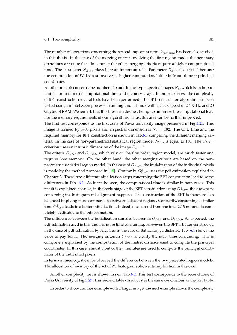
6.1 Tree complexity 151
The number of operations concerning the second important term Omerging has been also studied
in this thesis. In the case of the merging criteria involving the first region model the necessary
operations are quite fast. In contrast the other merging criteria require a higher computational
time. The parameter NBins plays here an important role. Parameter Ds is also critical because
the computation of Wilks’ test involves a higher computational time in front of more principal
coordinates.
Another remark concerns the number of bands in the hyperspectral images Nz , which is an impor-
tant factor in terms of computational time and memory usage. In order to assess the complexity
of BPT construction several tests have been performed. The BPT construction algorithm has been
tested using an Intel Xeon processor running under Linux with a clock speed of 2.40GHz and 20
Gbytes of RAM. We remark that this thesis mades no attempt to minimize the computational load
nor the memory requirements of our algorithms. Thus, this area can be further improved.
The first test corresponds to the first zone of Pavia university image presented in Fig.3.25. This
image is formed by 3705 pixels and a spectral dimension is Nz = 102. The CPU time and the
required memory for BPT construction is shown in Tab.6.1 comparing the different merging cri-
teria. In the case of non-parametrical statistical region model Nbins is equal to 150. The OMDS
criterion uses an intrinsic dimension of the image Ds = 3.
The criteria OSID and OSAM , which rely on the first order region model, are much faster and
requires low memory. On the other hand, the other merging criteria are based on the non-
parametric statistical region model. In the case of O1BAT , the initialization of the individual pixels
is made by the method proposed in [18]. Contrarily, O2BAT uses the pdf estimation explained in
Chapter 3. These two different initialization steps concerning the BPT construction lead to some
differences in Tab. 6.1. As it can be seen, the computational time is similar in both cases. This
result is explained because, in the early stage of the BPT construction using O1BAT , the drawback
concerning the histogram misalignment happens. The construction of the BPT is therefore less
balanced implying more comparisons between adjacent regions. Contrarily, consuming a similar
time O2BAT leads to a better initialization. Indeed, one second from the total 2.15 minutes is com-
pletely dedicated to the pdf estimation.
The differences between the initialization can also be seen in ODIF and OMDS . As expected, the
pdf estimation used in this thesis is more time consuming. However, the BPT is better constructed
in the case of pdf estimation by Alg. 1 as in the case of Battacharyya distance. Tab. 6.1 shows the
price to pay for it. The merging criterion OMDS is clearly the most time consuming. This is
completely explained by the computation of the matrix distance used to compute the principal
coordinates. In this case, almost 6 out of the 9 minutes are used to compute the principal coordi-
nates of the individual pixels.
In terms in memory, it can be observed the difference between the two presented region models.
The allocation of memory of the set of Nz histograms shows its implication in this case.
Another complexity test is shown in next Tab.6.2. This test corresponds to the second zone of
Pavia University of Fig.3.25 .This second table corroborates the same conclusions as the last Table.
In order to show another example with a larger image, the next example shows the complexity
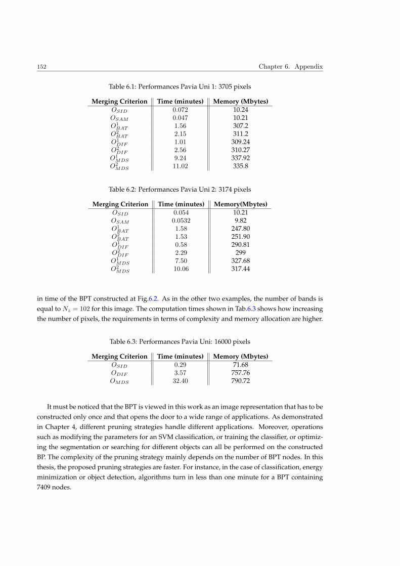
152 Chapter 6. Appendix
Table 6.1: Performances Pavia Uni 1: 3705 pixels
Merging Criterion Time (minutes) Memory (Mbytes)
OSID 0.072 10.24OSAM 0.047 10.21O1
BAT 1.56 307.2O2
BAT 2.15 311.2O1
DIF 1.01 309.24O2
DIF 2.56 310.27O1
MDS 9.24 337.92O2
MDS 11.02 335.8
Table 6.2: Performances Pavia Uni 2: 3174 pixels
Merging Criterion Time (minutes) Memory(Mbytes)
OSID 0.054 10.21OSAM 0.0532 9.82O1
BAT 1.58 247.80O2
BAT 1.53 251.90O1
DIF 0.58 290.81O2
DIF 2.29 299O1
MDS 7.50 327.68O2
MDS 10.06 317.44
in time of the BPT constructed at Fig.6.2. As in the other two examples, the number of bands is
equal to Nz = 102 for this image. The computation times shown in Tab.6.3 shows how increasing
the number of pixels, the requirements in terms of complexity and memory allocation are higher.
Table 6.3: Performances Pavia Uni: 16000 pixels
Merging Criterion Time (minutes) Memory (Mbytes)
OSID 0.29 71.68ODIF 3.57 757.76OMDS 32.40 790.72
It must be noticed that the BPT is viewed in this work as an image representation that has to be
constructed only once and that opens the door to a wide range of applications. As demonstrated
in Chapter 4, different pruning strategies handle different applications. Moreover, operations
such as modifying the parameters for an SVM classification, or training the classifier, or optimiz-
ing the segmentation or searching for different objects can all be performed on the constructed
BP. The complexity of the pruning strategy mainly depends on the number of BPT nodes. In this
thesis, the proposed pruning strategies are faster. For instance, in the case of classification, energy
minimization or object detection, algorithms turn in less than one minute for a BPT containing
7409 nodes.

6.2 Acronyms 153
6.2 Acronyms
BPT Binary Partition Tree
λ Wavenlength
Iλ Hyperspectral image
Nz Number of hyperspectral bands
Np Number of pixels of hyperspectral image
IλjHyperspectral image band given a specific wavelength λj
Iλj(p) the radiance value of the pixel p on the hyperspectral image band λj
Iλ(p) is the vector pixel p containing all the radiance values along the Nz wavelenghts
R Image region
P Image partition
NR Number of region containing in an image partition
RAG Region Adjacency Graph
N Tree node
TN Subtree rooted by BPT node N
MR Region Model
O(Ri, Rj) Merging criterion between region Ri and Rj
NRpNumber of spectra containing in region
IRλiThe average spectral value of a region R at the image band λi
IRλ Vector containing the average spectral values of a region R for all Nz bands
PR(λ) The probability distribution according to λ by applying the IRλ spectrum normalization
Hλk
R Empirical spatial distribution (histogram) of the region R in the band λk
NBins Number of bins
Hλi
R (Pak) Probability of the region R of having the radiance value ak in the band λi
P (p) Patch neighborhood centered at pixel p
Wx, Wy Horizontal and vertical dimension of patch neighborhood
Ωp Search window centered at p given its individual pixel distribution initialization
w(p, py) The additive contribution to the probability of the pixel p of having the value of Iλ(py).
dwin(p, py) The local displacement between pixels p and py according to the search window space Ωp
Z(p) Normalizing factor
dp The local displacement on the patch regarding the central pixel
hλiSmoothing parameter for λi
σλi
N Standard deviation of the noise in the λi
PR(λ) Probability distribution of a spectrum concerning λ dimension
SAM Spectral Angle Mapper
SID Spectral Information Divergence
D(Ri, Rj) Kullback-Leibler Divergence between Ri and Rj
BAT Battacharyya Distance
DIF Diffusion Distance
MDS Multidimensional Scaling Metric

154 Chapter 6. Appendix
P Image Partition
PGT Ground truth Partition
dasym Asymmetric distance between partitions
dsym Symmetric distance between partitions
Nc Number of classes of ground truth
AN Area of region contained on the node N
PN Class probability distribution of node N
LNiNumber of leaves forming the sub-tree TNi
rooted by the node Ni
EP Minimum Pruning cost of the partition P
C0 Equaltity constraint of the Lagrangia multiplier
EBPT the set of all the possible partitions P contained in the BPT
D(N ) Error commtited at node N
C(N ) Constraint at node N
λ∗ Optimal Lagrangian parameter
Nr and Nl Right and left children nodes sharing the same N father node
l Leaf node
WN Pruning decision weight for a node N
PNd (li) Local Pruning decision from a leaf li to its ancestor node on the branch N
B BPT branch
PB The set containing the nodes forming the BPT branch B
G Weighted graph
W Affinity matrix
d(Ni,Nj Similarity distance between node Ni andNj
L Laplacian matrix
E Second smallest eigenvalues of Laplacian matrix
NN Number of nodes forming a BPT branch

6.3 Mathematical Appendix: Association measures 155
6.3 Mathematical Appendix: Association measures
Roy, Lawley-Hotelling and Pillai Criteria
For testing β = 0, another criteria as the Roy R, Lawley-Hotelling U and Pilllai’s criterion V can
be employed as
R =λ1
(1 + λ1)(6.5)
U = tr(E−1H) =
DsX
i=1
λi (6.6)
V = tr((E +H)−1H) =
DsX
i=1
λi
(1 + λi)(6.7)
where λ are the eigenvalues associated to E−1H . These criteria can be described in terms of
canonical correlations as
R = r21 (6.8)
U =
DsX
i=1
r2i1− r2i
(6.9)
V =
DsX
i=1
r2i (6.10)
The three different tests can be used to define three new association measures AR, ALH and
AP by
AR =λ1
(1 + λ1)(6.11)
ALH =U
Ds
(1 +U
Ds
) (6.12)
AP =V
Ds
(6.13)
Other symmetric measures to measure multivariate dependence between two
data sets
Vector Correlations
Given two data sets X and Y whose covariance matrices are defined by Sxx = XtX , Syy = Y Y t
and SX,y = XtY , the RV coefficient [25] is given by
156 Chapter 6. Appendix
RV (X,Y ) =tr(SxySyx)
q
tr(S2xx)tr(S
2yy)
(6.14)
In our case, being URiand URj
the standard coordinates of two regions having NzxDs di-
mensions, Sxx = Syy = IDswhere IDs
is a diagonal matrix of Ds columns and rows. Thus, the
association measure ARV given by the vectorial correlation between two regions Ri and Rj is
ARV (Ri, Rj) =tr(U t
RiURj
U tRj
URi)
p
D2s
(6.15)
which is expressed in terms of canonical correlations ri as
ARV (Ri, Rj) =
DsX
i=1
r2i
Ds
(6.16)
Note that being in our case tr(S2xx) = tr(S2
yy), the association measure ARV is equal to AP
Generalized multiple Correlation
Another measure of multiple correlation coefficient [31] between X and Y has been defined as
R2(X,Y ) =det(SyxS
−1xx Sxy)
det(Syy)(6.17)
Simplifying this last equation when X and Y correspond to the standard coordinates URiand
URj, the association measure AR by the multiple correlation coefficient is defined as
AHC(Ri, Rj) = det(U tRj
URiU tRiURj
) =
DsY
i=1
r2i (6.18)
where notation HC refers to Hotelling and Cramer[31]
Procrustes statistics
According to [28], Procrustes analysis is a technique which matches a configuration to another,
where there is a one-to-one correspondence from one set to the other set of points, and obtains a
measure of the match. If both configurations are represented by two centered matrices X and Y,
the Procrustes statistic PR is
PR2(X,Y ) =[tr(XtY Y tX)
12 ]2
tr(XtX)tr(Y tY )(6.19)
This test can be expressed as the association measure APR by considering Y = URjΛRj
and
X = URiΛRi
as

6.3 Mathematical Appendix: Association measures 157
APR(Ri, Rj) =[tr(ΛRi
UtRi
URjΛ2
RjUt
RjURi
ΛRi)12 ]2
tr(Λ2Ri
)tr(Λ2Rj
)
=[tr(Ut
RiURj
UtRj
URi)12 ]2
D2s
=
(
DsX
i=1
ri)2
Ds(6.20)
Order relationship
The association measures can be ordered as
AHC ≤ APR ≤ AP ≤ ALH ≤ AR ≤ Aw (6.21)
because, clearly,
DsY
i=1
r2i ≤
DsY
i=1
(r2i )1s ≤
DsX
i=1
r2i
Ds
(6.22)
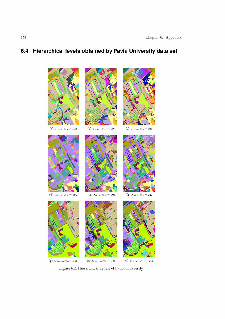
158 Chapter 6. Appendix
6.4 Hierarchical levels obtained by Pavia University data set
(a) OSID , NR = 102 (b) OSID , NR = 186 (c) OSID , NR = 242
(d) ODIF , NR = 102 (e) ODIF , NR = 186 (f) ODIF , NR = 242
(g) OMDS , NR = 102 (h) OMDS , NR = 186 (i) OMDS , NR = 242
Figure 6.2: Hierarchical Levels of Pavia University

6.5 List of Publications 159
6.5 List of Publications
International Journals
• A. Alonso-Gonzalez, S. Valero, J. Chanussot, C. Lopez-Martinez and P. Salembier,
Processing multidimensional SAR and hyperspectral images with Binary Partition Trees,
In reviewing process in IEEE Transactions on Geoscience and Remote Sensing, 2012
• S. Valero, P. Salembier and J. Chanussot,
Hyperspectral image representation and processing with Binary Partition Trees,
In reviewing process in IEEE Transactions on Image Processing, 2011
• C.M. Cuadras, S. Valero, D. Cuadras, P. Salembier and J. Chanussot,
Distance-based measure of association with applications in relating hyperspectral images,
Communications in Statistics: Theory and Methods,vol.41, pp. 2342–2355, 2012.
International Conferences
• S. Valero, P. Salembier and J. Chanussot,
Hyperspectral image segmentation using Binary Partition Trees,
IEEE ICIP’11 - International Conference on Image Processing, september 2011
• S. Valero, P. Salembier, J. Chanussot and C.M. Cuadras,
Improved Binary Partition Tree Construction for hyperspectral images: Application to object detec-
tion
IEEE IGARSS’11 - International Geoscience and Remote Sensing Symposium, Vancouver
• J.Benediktsson, L.Bruzzone, J.Chanussot, M.Dalla Mura, P.Salembier and S.Valero,
Hierarchical Analysis of Remote Sensing Data: Morphological Attribute Profiles and Binary Parti-
tion Trees
ISMM 2011, International Symposium on Mathematical Morphology, 2011
• C.M. Cuadras, S. Valero, P. Salembier, J. Chanussot
Some measures of multivariate association relating two spectral data sets,
COMPSTAT 2010 - International Conference on Computational Statistics, 2010, Paris
• S. Valero, P. Salembier and J. Chanussot,
Comparison of merging orders and pruning strategies for binary partition tree in HSI data
IEEE ICIP’10 - International Conference on Image Processing, 2010, Hong Kong
• S. Valero, P. Salembier and J. Chanussot,
New hyperspectral data representation using binary partition tree
IEEE IGARSS’10 - International Geoscience and Remote Sensing Symposium,2010, USA
This paper received the Symposium Prize Best Paper Award

160 Chapter 6. Appendix
National Conferences
• S. Valero, P. Salembier and J. Chanussot,
L’arbre binaire de partitions: Une nouvelle representation hierarchique d’une image hyperspectral,
Gretsi, Symposium on Signal and Image Processing, 2011

7Résumé en français

162 Chapter 7. Résumé en français
L’Arbre Binaire de Partitions: Un nouvel outil pour
la représentation hiérarchique et l’analyse des
images hyperspectrales
14 février 2013
Table des matières
1 Introduction 2
2 La construction de l’Arbre Binaire de Partitions 6
2.1 Le modèle paramétrique de premier ordre . . . . . . . . . . . . . . . . . . . 7
2.1.1 Spectral Information Divergence (SID) . . . . . . . . . . . . . . . . 8
2.2 Le modèle statistique non paramétrique . . . . . . . . . . . . . . . . . . . . 8
2.2.1 Bhattacharyya distance . . . . . . . . . . . . . . . . . . . . . . . . . 9
2.2.2 Diffusion Distance . . . . . . . . . . . . . . . . . . . . . . . . . . . . 9
2.2.3 Association measure via Multidimensional Scaling . . . . . . . . . . 10
3 Évaluation de la construction de l’ABP 13
4 L’élagage de l ’ABP 17
4.1 La classification supervisée . . . . . . . . . . . . . . . . . . . . . . . . . . . . 17
4.1.1 Calcul des descripteurs . . . . . . . . . . . . . . . . . . . . . . . . . . 17
4.1.2 L’analyse des branches . . . . . . . . . . . . . . . . . . . . . . . . . . 18
4.2 La segmentation supervisée . . . . . . . . . . . . . . . . . . . . . . . . . . . 21
4.3 La détéction d’objets . . . . . . . . . . . . . . . . . . . . . . . . . . . . . . . 25
4.3.1 La détection de routes . . . . . . . . . . . . . . . . . . . . . . . . . . 26
4.3.2 La détection des bâtiments . . . . . . . . . . . . . . . . . . . . . . . 27
5 Conclusions 28
1
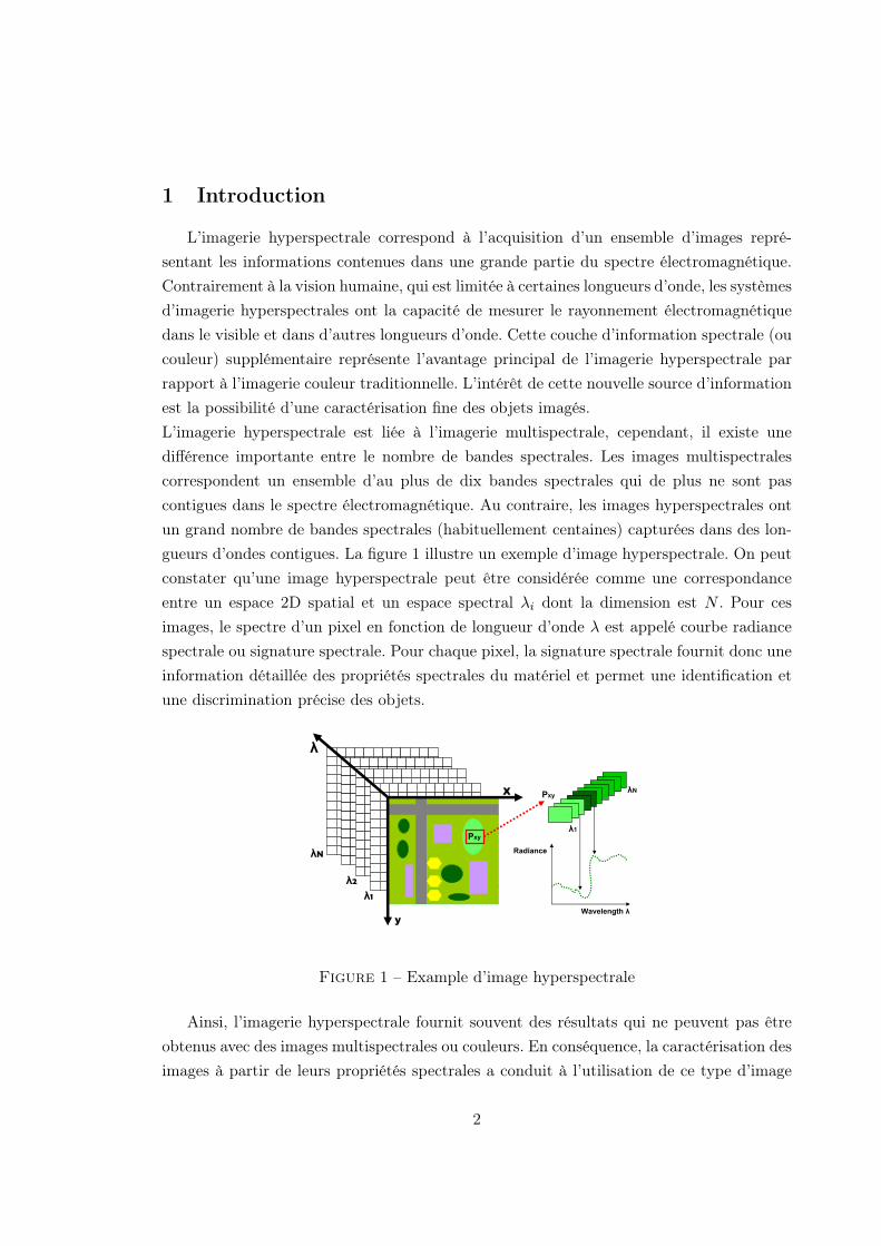
1 Introduction
L’imagerie hyperspectrale correspond à l’acquisition d’un ensemble d’images repré-
sentant les informations contenues dans une grande partie du spectre électromagnétique.
Contrairement à la vision humaine, qui est limitée à certaines longueurs d’onde, les systèmes
d’imagerie hyperspectrales ont la capacité de mesurer le rayonnement électromagnétique
dans le visible et dans d’autres longueurs d’onde. Cette couche d’information spectrale (ou
couleur) supplémentaire représente l’avantage principal de l’imagerie hyperspectrale par
rapport à l’imagerie couleur traditionnelle. L’intérêt de cette nouvelle source d’information
est la possibilité d’une caractérisation fine des objets imagés.
L’imagerie hyperspectrale est liée à l’imagerie multispectrale, cependant, il existe une
différence importante entre le nombre de bandes spectrales. Les images multispectrales
correspondent un ensemble d’au plus de dix bandes spectrales qui de plus ne sont pas
contigues dans le spectre électromagnétique. Au contraire, les images hyperspectrales ont
un grand nombre de bandes spectrales (habituellement centaines) capturées dans des lon-
gueurs d’ondes contigues. La figure 1 illustre un exemple d’image hyperspectrale. On peut
constater qu’une image hyperspectrale peut être considérée comme une correspondance
entre un espace 2D spatial et un espace spectral λi dont la dimension est N . Pour ces
images, le spectre d’un pixel en fonction de longueur d’onde λ est appelé courbe radiance
spectrale ou signature spectrale. Pour chaque pixel, la signature spectrale fournit donc une
information détaillée des propriétés spectrales du matériel et permet une identification et
une discrimination précise des objets.
X
y
そ
そ!"そ#
そ$"
!"#
$%&'%()*
+%,*-*(./01そ
そ2
そ3!"#
Figure 1 – Example d’image hyperspectrale
Ainsi, l’imagerie hyperspectrale fournit souvent des résultats qui ne peuvent pas être
obtenus avec des images multispectrales ou couleurs. En conséquence, la caractérisation des
images à partir de leurs propriétés spectrales a conduit à l’utilisation de ce type d’image
2
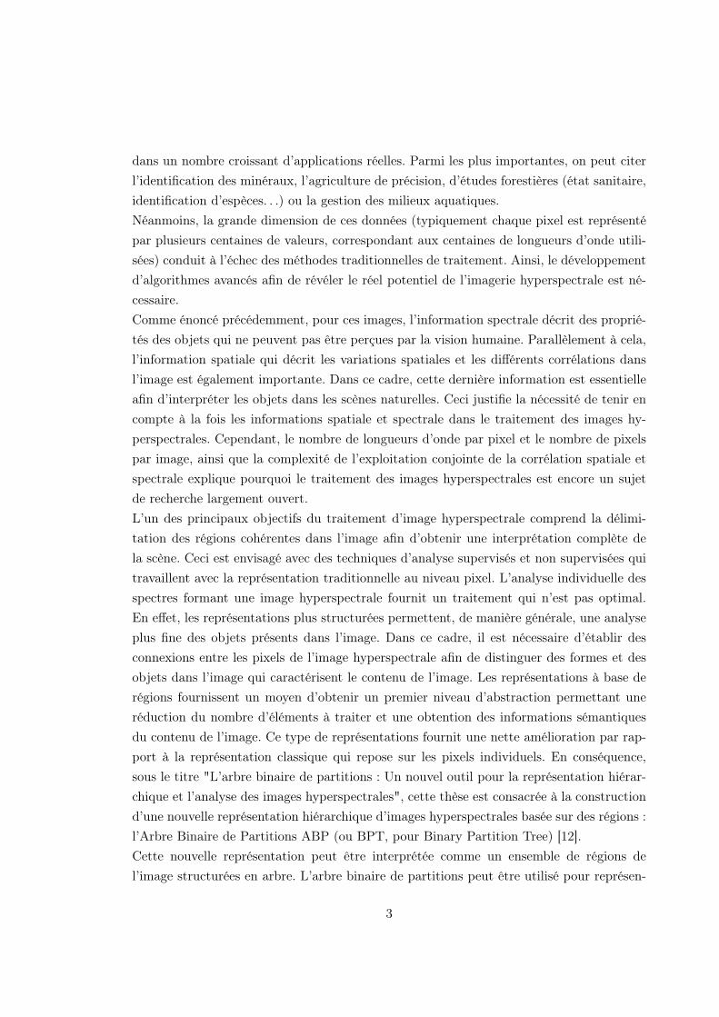
dans un nombre croissant d’applications réelles. Parmi les plus importantes, on peut citer
l’identification des minéraux, l’agriculture de précision, d’études forestières (état sanitaire,
identification d’espèces. . .) ou la gestion des milieux aquatiques.
Néanmoins, la grande dimension de ces données (typiquement chaque pixel est représenté
par plusieurs centaines de valeurs, correspondant aux centaines de longueurs d’onde utili-
sées) conduit à l’échec des méthodes traditionnelles de traitement. Ainsi, le développement
d’algorithmes avancés afin de révéler le réel potentiel de l’imagerie hyperspectrale est né-
cessaire.
Comme énoncé précédemment, pour ces images, l’information spectrale décrit des proprié-
tés des objets qui ne peuvent pas être perçues par la vision humaine. Parallèlement à cela,
l’information spatiale qui décrit les variations spatiales et les différents corrélations dans
l’image est également importante. Dans ce cadre, cette dernière information est essentielle
afin d’interpréter les objets dans les scènes naturelles. Ceci justifie la nécessité de tenir en
compte à la fois les informations spatiale et spectrale dans le traitement des images hy-
perspectrales. Cependant, le nombre de longueurs d’onde par pixel et le nombre de pixels
par image, ainsi que la complexité de l’exploitation conjointe de la corrélation spatiale et
spectrale explique pourquoi le traitement des images hyperspectrales est encore un sujet
de recherche largement ouvert.
L’un des principaux objectifs du traitement d’image hyperspectrale comprend la délimi-
tation des régions cohérentes dans l’image afin d’obtenir une interprétation complète de
la scène. Ceci est envisagé avec des techniques d’analyse supervisés et non supervisées qui
travaillent avec la représentation traditionnelle au niveau pixel. L’analyse individuelle des
spectres formant une image hyperspectrale fournit un traitement qui n’est pas optimal.
En effet, les représentations plus structurées permettent, de manière générale, une analyse
plus fine des objets présents dans l’image. Dans ce cadre, il est nécessaire d’établir des
connexions entre les pixels de l’image hyperspectrale afin de distinguer des formes et des
objets dans l’image qui caractérisent le contenu de l’image. Les représentations à base de
régions fournissent un moyen d’obtenir un premier niveau d’abstraction permettant une
réduction du nombre d’éléments à traiter et une obtention des informations sémantiques
du contenu de l’image. Ce type de représentations fournit une nette amélioration par rap-
port à la représentation classique qui repose sur les pixels individuels. En conséquence,
sous le titre "L’arbre binaire de partitions : Un nouvel outil pour la représentation hiérar-
chique et l’analyse des images hyperspectrales", cette thèse est consacrée à la construction
d’une nouvelle représentation hiérarchique d’images hyperspectrales basée sur des régions :
l’Arbre Binaire de Partitions ABP (ou BPT, pour Binary Partition Tree) [12].
Cette nouvelle représentation peut être interprétée comme un ensemble de régions de
l’image structurées en arbre. L’arbre binaire de partitions peut être utilisé pour représen-
3
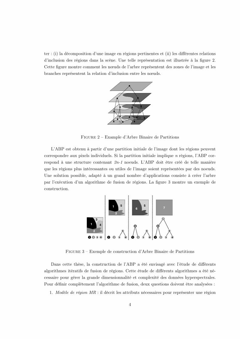
ter : (i) la décomposition d’une image en régions pertinentes et (ii) les différentes relations
d’inclusion des régions dans la scène. Une telle représentation est illustrée à la figure 2.
Cette figure montre comment les nœuds de l’arbre représentent des zones de l’image et les
branches représentent la relation d’inclusion entre les nœuds.
Figure 2 – Example d’Arbre Binaire de Partitions
L’ABP est obtenu à partir d’une partition initiale de l’image dont les régions peuvent
correspondre aux pixels individuels. Si la partition initiale implique n régions, l’ABP cor-
respond à une structure contenant 2n-1 noeuds. L’ABP doit être créé de telle manière
que les régions plus intéressantes ou utiles de l’image soient représentées par des noeuds.
Une solution possible, adapté à un grand nombre d’applications consiste à créer l’arbre
par l’exécution d’un algorithme de fusion de régions. La figure 3 montre un exemple de
construction.
1
2
3
4
1
2
56
5
3 4
5
1 23 41 2 3 4
5
1 2
6
7
3 4
5
1 2
6
7
Original Partition
Figure 3 – Exemple de construction d’Arbre Binaire de Partitions
Dans cette thèse, la construction de l’ABP a été envisagé avec l’étude de différents
algorithmes itératifs de fusion de régions. Cette étude de différents algorithmes a été né-
cessaire pour gérer la grande dimensionnalité et complexité des données hyperspectrales.
Pour définir complètement l’algorithme de fusion, deux questions doivent être analysées :
1. Modèle de région MR : il décrit les attributs nécessaires pour représenter une région
4
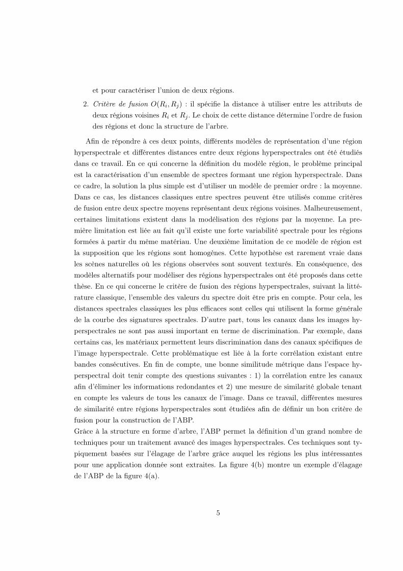
et pour caractériser l’union de deux régions.
2. Critère de fusion O(Ri, Rj) : il spécifie la distance à utiliser entre les attributs de
deux régions voisines Ri et Rj . Le choix de cette distance détermine l’ordre de fusion
des régions et donc la structure de l’arbre.
Afin de répondre à ces deux points, différents modèles de représentation d’une région
hyperspectrale et différentes distances entre deux régions hyperspectrales ont été étudiés
dans ce travail. En ce qui concerne la définition du modèle région, le problème principal
est la caractérisation d’un ensemble de spectres formant une région hyperspectrale. Dans
ce cadre, la solution la plus simple est d’utiliser un modèle de premier ordre : la moyenne.
Dans ce cas, les distances classiques entre spectres peuvent être utilisés comme critères
de fusion entre deux spectre moyens représentant deux régions voisines. Malheureusement,
certaines limitations existent dans la modélisation des régions par la moyenne. La pre-
mière limitation est liée au fait qu’il existe une forte variabilité spectrale pour les régions
formées à partir du même matériau. Une deuxième limitation de ce modèle de région est
la supposition que les régions sont homogènes. Cette hypothèse est rarement vraie dans
les scènes naturelles où les régions observées sont souvent texturés. En conséquence, des
modèles alternatifs pour modéliser des régions hyperspectrales ont été proposés dans cette
thèse. En ce qui concerne le critère de fusion des régions hyperspectrales, suivant la litté-
rature classique, l’ensemble des valeurs du spectre doit être pris en compte. Pour cela, les
distances spectrales classiques les plus efficaces sont celles qui utilisent la forme générale
de la courbe des signatures spectrales. D’autre part, tous les canaux dans les images hy-
perspectrales ne sont pas aussi important en terme de discrimination. Par exemple, dans
certains cas, les matériaux permettent leurs discrimination dans des canaux spécifiques de
l’image hyperspectrale. Cette problématique est liée à la forte corrélation existant entre
bandes consécutives. En fin de compte, une bonne similitude métrique dans l’espace hy-
perspectral doit tenir compte des questions suivantes : 1) la corrélation entre les canaux
afin d’éliminer les informations redondantes et 2) une mesure de similarité globale tenant
en compte les valeurs de tous les canaux de l’image. Dans ce travail, différentes mesures
de similarité entre régions hyperspectrales sont étudiées afin de définir un bon critère de
fusion pour la construction de l’ABP.
Grâce à la structure en forme d’arbre, l’ABP permet la définition d’un grand nombre de
techniques pour un traitement avancé des images hyperspectrales. Ces techniques sont ty-
piquement basées sur l’élagage de l’arbre grâce auquel les régions les plus intéressantes
pour une application donnée sont extraites. La figure 4(b) montre un exemple d’élagage
de l’ABP de la figure 4(a).
5
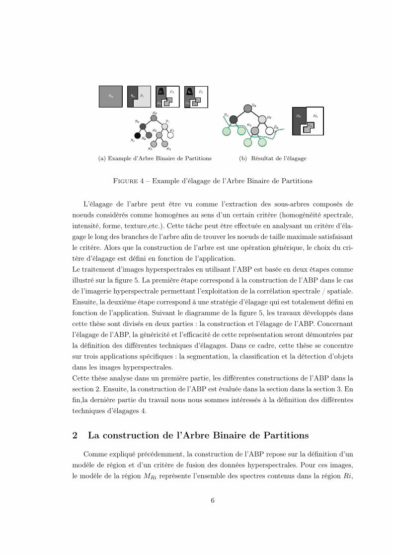
(a) Example d’Arbre Binaire de Partitions (b) Résultat de l’élagage
Figure 4 – Example d’élagage de l’Arbre Binaire de Partitions
L’élagage de l’arbre peut être vu comme l’extraction des sous-arbres composés de
noeuds considérés comme homogènes au sens d’un certain critère (homogénéité spectrale,
intensité, forme, texture,etc.). Cette tâche peut être effectuée en analysant un critère d’éla-
gage le long des branches de l’arbre afin de trouver les noeuds de taille maximale satisfaisant
le critère. Alors que la construction de l’arbre est une opération générique, le choix du cri-
tère d’élagage est défini en fonction de l’application.
Le traitement d’images hyperspectrales en utilisant l’ABP est basée en deux étapes comme
illustré sur la figure 5. La première étape correspond à la construction de l’ABP dans le cas
de l’imagerie hyperspectrale permettant l’exploitation de la corrélation spectrale / spatiale.
Ensuite, la deuxième étape correspond à une stratégie d’élagage qui est totalement défini en
fonction de l’application. Suivant le diagramme de la figure 5, les travaux développés dans
cette thèse sont divisés en deux parties : la construction et l’élagage de l’ABP. Concernant
l’élagage de l’ABP, la généricité et l’efficacité de cette représentation seront démontrées par
la définition des différentes techniques d’élagages. Dans ce cadre, cette thèse se concentre
sur trois applications spécifiques : la segmentation, la classification et la détection d’objets
dans les images hyperspectrales.
Cette thèse analyse dans un première partie, les différentes constructions de l’ABP dans la
section 2. Ensuite, la construction de l’ABP est évaluée dans la section dans la section 3. En
fin,la dernière partie du travail nous nous sommes intéressés à la définition des différentes
techniques d’élagages 4.
2 La construction de l’Arbre Binaire de Partitions
Comme expliqué précédemment, la construction de l’ABP repose sur la définition d’un
modèle de région et d’un critère de fusion des données hyperspectrales. Pour ces images,
le modèle de la région MRi représente l’ensemble des spectres contenus dans la région Ri,
6
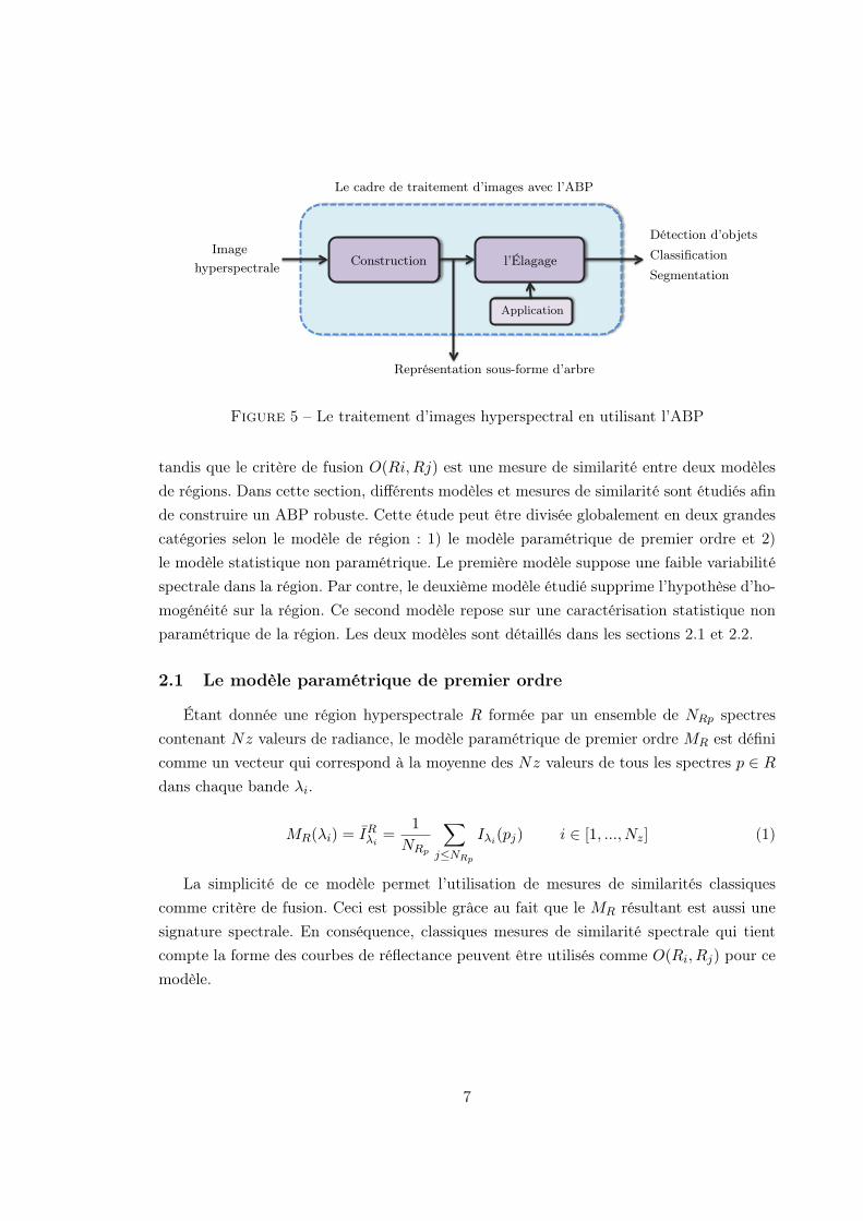
!!
!! !!
!!
Construction l’Élagage
Le cadre de traitement d’images avec l’ABP
Représentation sous-forme d’arbre
Application
Image
hyperspectraleClassification
Segmentation
Détection d’objets
Figure 5 – Le traitement d’images hyperspectral en utilisant l’ABP
tandis que le critère de fusion O(Ri,Rj) est une mesure de similarité entre deux modèles
de régions. Dans cette section, différents modèles et mesures de similarité sont étudiés afin
de construire un ABP robuste. Cette étude peut être divisée globalement en deux grandes
catégories selon le modèle de région : 1) le modèle paramétrique de premier ordre et 2)
le modèle statistique non paramétrique. Le première modèle suppose une faible variabilité
spectrale dans la région. Par contre, le deuxième modèle étudié supprime l’hypothèse d’ho-
mogénéité sur la région. Ce second modèle repose sur une caractérisation statistique non
paramétrique de la région. Les deux modèles sont détaillés dans les sections 2.1 et 2.2.
2.1 Le modèle paramétrique de premier ordre
Étant donnée une région hyperspectrale R formée par un ensemble de NRp spectres
contenant Nz valeurs de radiance, le modèle paramétrique de premier ordre MR est défini
comme un vecteur qui correspond à la moyenne des Nz valeurs de tous les spectres p ∈ R
dans chaque bande λi.
MR(λi) = IRλi=
1
NRp
X
j≤NRp
Iλi(pj) i ∈ [1, ..., Nz] (1)
La simplicité de ce modèle permet l’utilisation de mesures de similarités classiques
comme critère de fusion. Ceci est possible grâce au fait que le MR résultant est aussi une
signature spectrale. En conséquence, classiques mesures de similarité spectrale qui tient
compte la forme des courbes de réflectance peuvent être utilisés comme O(Ri, Rj) pour ce
modèle.
7
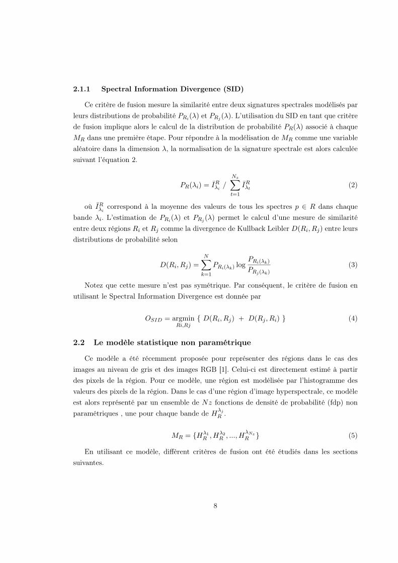
2.1.1 Spectral Information Divergence (SID)
Ce critère de fusion mesure la similarité entre deux signatures spectrales modélisés par
leurs distributions de probabilité PRi(λ) et PRj
(λ). L’utilisation du SID en tant que critère
de fusion implique alors le calcul de la distribution de probabilité PR(λ) associé à chaque
MR dans une première étape. Pour répondre à la modélisation de MR comme une variable
aléatoire dans la dimension λ, la normalisation de la signature spectrale est alors calculée
suivant l’équation 2.
PR(λi) = IRλi/
NzX
t=1
IRλt(2)
où IRλicorrespond à la moyenne des valeurs de tous les spectres p ∈ R dans chaque
bande λi. L’estimation de PRi(λ) et PRj
(λ) permet le calcul d’une mesure de similarité
entre deux régions Ri et Rj comme la divergence de Kullback Leibler D(Ri, Rj) entre leurs
distributions de probabilité selon
D(Ri, Rj) =NX
k=1
PRi(λk) logPRi(λk)
PRj(λk)(3)
Notez que cette mesure n’est pas symétrique. Par conséquent, le critère de fusion en
utilisant le Spectral Information Divergence est donnée par
OSID = argminRi,Rj
D(Ri, Rj) + D(Rj , Ri) (4)
2.2 Le modèle statistique non paramétrique
Ce modèle a été récemment proposée pour représenter des régions dans le cas des
images au niveau de gris et des images RGB [1]. Celui-ci est directement estimé à partir
des pixels de la région. Pour ce modèle, une région est modélisée par l’histogramme des
valeurs des pixels de la région. Dans le cas d’une région d’image hyperspectrale, ce modèle
est alors représenté par un ensemble de Nz fonctions de densité de probabilité (fdp) non
paramétriques , une pour chaque bande de Hλj
R .
MR = Hλ1
R , Hλ2
R , ..., HλNz
R (5)
En utilisant ce modèle, diffèrent critères de fusion ont été étudiés dans les sections
suivantes.
8
2.2.1 Bhattacharyya distance
La classique Bhattacharyya distance entre deux statistiques des distributions discrètes
mesure la quantité de chevauchement entre eux. Etant donnée deux régions adjacentes Ri
et Rj , définies par leur modèles statistiques non-paramétriques de l’équation 5, la distance
Battacharyya à la bande λk entre les distributions de Hλk
Riet Hλk
Rjest définie par
BC(Hλk
Ri, Hλk
Rj) = − log(
NBinsX
s=1
Hλk
Ri(as)
1
2Hλk
Rj(as)
1
2 ) (6)
où NBins sont le nombre de cases utilisées pour quantifier les intensités des images.
Notez que si Hλk
Riet Hλk
Rjrecouvrent parfaitement, la distance de Bhattacharyya est alors
0. D’autre part, en utilisant l’équation 6, la similitude entre deux régions hyperspectrales
est seulement calculée pour une bande spécifique λk.
Dans notre cas, MRiet MRj
sont constitués par un ensemble de distributions Nz. Par
conséquent, le critère de la fusion OBAT peut être définie comme la somme de Nz mesures
obtenues pour les différentes bandes.
OBAT = argminRi,Rj
NX
k=1
BC(Hλk
Ri, Hλk
Rj) (7)
La distance décrit ci-dessus suppose que les histogrammes sont déjà alignés. Cela im-
plique que ce critère de fusion est sensible aux distorsions, et souffre de l’effet de quanti-
fication. Pour résoudre ce problème, l’utilisation d’une mesure de similarité inter-bin est
proposée dans la section suivante. Cela correspond a la distance de diffusion utilisé ici
comme critère de fusion.
2.2.2 Diffusion Distance
La distance de diffusion DK est une distance inter-bin qui mesure la différence entre
deux histogrammes à des échelles de résolution différentes grâce à un processus de diffusion
[11]. L’objectif de mesurer les histogrammes aux différentes échelles consiste à penser que
si les histogrammes sont différents, la différence entre eux existent dans plusieurs échelles.
Le processus de diffusion est calculé par la convolution de la différence histogramme dl(AS)
avec un filtre gaussien φσG(as), ou as ∈ Rm est un vecteur. Ainsi, chaque échelle de diffusion
l correspond a deux tâches : la convolution avec le filtre gaussien et une étape de sous-
échantillonnage en tant que :
9
d0(as) = Hλk
Ri(as)−Hλk
Rj(as) (8)
dl(as) = [dl−1(as) ∗ φσG(as)] ↓2 l ∈ [1, ..., L] (9)
La notation ↓2 correspond au sous-échantillonnage par une facteur deux. L est le nombre
d’échelles étudiées et σG est l’écart type du filtre gaussien φ. En utilisant l’équation 9, la
distance DK entre deux histogrammes peut être calculée comme la norme L1 à différents
niveaux
DK(Hλk
Ri, Hλk
Rj) =
LX
l=0
NBX
s=1
|dl(as)| (10)
Par conséquent, le critère proposé de fusionner l’aide de la distance de diffusion défini
dans les équations précédentes est calculée comme :
ODIF = argminRi,Rj
NX
k=1
DK(Hλk
Ri, Hλk
Rj) (11)
À ce point, il convient de rappeler que les bandes hyperspectrales sont traitées séparé-
ment par les deux derniers critères : OBAT et ODIF . Cela implique que la corrélation entre
les bandes n’est pas prise en compte dans ces critères de fusion. En plus, la forme spectrale
globale des spectres est une autre information qui n’est pas utilisée. Pour contourner ces
limitations, un dernier critère de fusion est proposée dans la section 2.2.3.
2.2.3 Association measure via Multidimensional Scaling
Le critère de fusion proposé ici est divisé en deux étapes [7, 15]. En analysant les
relations de similarité inter-bande de chaque modèle de région MR, la première étape cor-
respond à une réduction local de la dimension. L’objectif de cette étape est d’éliminer les
informations redondantes en utilisant une analyse d’échelle métrique multidimensionnelle
(MDS) [5]. En conséquence, les composantes principales de chaque modèle de région conte-
nant les informations les plus pertinentes sont obtenues. Ensuite, une mesure de similarité
mesurant la corrélation des deux ensembles de données obtenus via le MDS est effectuée
comme deuxième étape. Cette mesure de similarité, repose sur une test statistique sur
l’analyse de variance multivariée (MANOVA). L’objectif est de tester si il y a une dépen-
dance (ou de corrélation) entre les composantes principales.
Première étape : La reduction local de la dimension en utilisant le MDS
10
L’objectif du multidimensional scaling est de construire une représentation euclidienne des
individus dans un espace de dimension réduite qui approche au "mieux" les indices obser-
vées . Dans notre cas, le MDS tente de réduire la dimension formé par les Nz distributions
de probabilité de chaque MR. Pour l’exécuter, les similitudes de distribution de probabilité
(ou dissimilarités) de MR peut être représenté par une Nz ×Nz de distance matrice ∆R=
(δkl), ouδkl = δlk ≥0 est la distance de diffusion calculé par l’équation 11. Par conséquent,
étant A la matrice de terme générale A = −(12)δ2kl et H = IN −
1N110 la matrice de cen-
trage, le calcul de la matrice des produits scalaires par double centrage BR associée à ∆R
est calculée comme BR = HAH pour chaque MR . La matrice des produits scalaires BR
est une Nz × Nz matrice symétrique dont décomposition spectrale est BR = URΛ2RU
0R.
En supposant que les valeurs propres de λR sont disposés dans l’ordre décroissant, les
matrices URλR et UR contenant les coordonnées principales et standards de la région R,
respectivement. Ensuite, l’intérêt du MDS consiste à prendre les Ds coordonnées le plus
représentatives de chaque MR.
Compte tenu deux régions définies par MRiet MRj
, notre intérêt est de mesurer la simi-
larité entre leurs Ds premières coordonnées standard. Par conséquent, deux matrices de
distance ∆Riet ∆Rj
pour trouver BRi= URi
Λ2RiU 0Ri
and BRj= URj
Λ2RjU 0Rj
devrait être
calculée en utilisant la procédure expliquée.
Le nombre des dimensions à utiliser Ds est un aspect important dans la plupart des mé-
thodes d’analyse multivariée. Dans le cas du MDS, la sélection de Ds est basé sur le
pourcentage de la variabilité existant dans les premières dimensions des coordonnées prin-
cipales. Ici, un critère étendant celui proposé dans est utilisé pour définir la valeur de Ds
[8]. Tout d’abord, un certain nombre de dimensions Ns suggéré par les données est fixé.
Puis, étant ui et vi, i = 1, ..., Ns, les premières Ns colonnes de URiet URj
, la séquence Ck
est définie comme
Ck =
Pkt=1
Pkp=1
λ2
tRi(u0
tvp)2λ2
tRjPNs
t=1
PNsp=1
λ2
tRi(u0
tvp)2λ2
tRj
k 2 [1, ..., Ns] (12)
où λ2tRi
λ2tRj
sont les valeurs propres de BRiand BRj
qui sont proportionnelle à la va-
riance des axes principaux correspondants. Ici Ns st la dimension minimale pour laquellePNs
t=1λ2
tRPNt=1
λ2
tR
≈ 1 et (u0tvp)2 est le coefficient de corrélation entre les t-ème et p-ème coordonnées.
. Ainsi, le numérateur Ck est une moyenne pondérée des relations entre les axes principaux.
Il est clair que 0 ≤ C1 ≤, ... ≤ CDs ≤, ... ≤ CNs = 1. La dimension Ds est alors choisie
telle que CDs est élevée, par exemple CDs = 0.9.
Deuxieme étape : Measure de similarité entre les Ds coordonées principales de
MRiet MRj
11
Un test statistique pour mesurer la similarité entre les régions définies par leurs coordonnées
principales peut être défini considérant les colonnes Ds de URiΛRi
and URjΛRj
comme
comme un prédicteur X et une réponse Y d’un modèle de régression linéaire multivariée
définie par
Y = Xβ + e (13)
où β est la matrice de paramètres contenant les coefficients de régression et e est la
matrice d’erreurs. L’estimation des moindres carrés β est donné par β = (X 0X)−1X 0Y et
la matrice de prédiction est Y = Xβ = PY étant donné P = (X 0X)−1X la matrice de
régression. Il est clair que s’il n’y a pas de relation entre X et Y, la matrice β est égal à
0. Considérant cela, l’idée est d’effectuer un test de vérification de l’hypothèse β = 0 pour
mesurer si existe une relation significative entre X et Y .
Dans cette étude, le test du rapport de vraisemblance W (où lamba Wilks) est proposé pour
mesurer si l’ hypothèse β = 0 est vraie ou fausse. Dans notre cas, Y et X correspondent
aux Y = URjΛRj
et X = URiΛRi
. Alors, le modèle prédit correspond à Y = PY =
URiU 0RiURj
ΛRj. L’équation 14 est alors définie à l’aide de E = ΛRj
(I−U 0RjURi
U 0RiURj
)ΛRj
et E+H = Y 0Y = ΛRjU 0RjURj
ΛRj= Λ
2Rj
. Ces deux dernières équations définissent le test
de lambda Wilks W (Ri, Rj) comme
W (Ri, Rj) = det(E)/det(E +H) = det(I − U 0RjURi
U 0RiURj
) (14)
Le critère de l’équation peut également être définie par W (Ri, Rj) = λ1w × λ2
w.... × λDsw
où λiw sont les valeurs propres correspondant à
det(E − λw(E +H)) = 0 (15)
Étant 0 ≤ λiw ≤ 1, le carré de la corrélation canonique r2i est définie par 1 − λi
w. Le
critère de Wilks peut donc être exprimée en termes de corrélations canoniques [6] comme
W (Ri, Rj) =
DsY
i=1
(1− r2i ) (16)
L’équation dernière satisfait que 0 ≤ W (Ri, Rj) ≤ 1 et W (Ri, Rj) = 1 si Ri est égal à
Rj . Celui-ci conduit à la définition de critère de fusion comme
OMDS = argminRi,Rj
W (Ri, Rj) (17)
12
3 Évaluation de la construction de l’ABP
Cette expérience évalue les partitions obtenues pendant dans la construction de l’ABP.
Les partitions obtenues dans la création de l’arbre permettent de faire une première évalua-
tion des modèles de la région et les critères de fusion proposées dans la section précédente.
Dans la construction de l’arbre, une partition initiale est composée de Np régions formées
par de pixels individuels. Pour tant, afin d’obtenir une partition avec NR régions , un
nombre de Np − NR fusions doivent être accomplies. La qualité des partitions ayant NR
régions est alors évaluée avec deux distances différentes. Ces deux mesures ont été définies
dans le cadre de la segmentation d’images et déjà utilisé dans [1] [3]
La première mesure de qualité est la distance de asymétrique dasy qui est comprise entre 0
et 1. Cette distance mesure le nombre minimum de pixels dont l’étiquette doit être modifiée
de sorte que la partition P1 devient plus fine que la partition P2, normalisé par le nombre
total de pixels de l’image moins un. Si P1 est la vérité du terrain et P2 est la partition
calculée, Dasy(P1, P2) mesure la sous-segmentation et dasy(P2, P1) la sur-segmentation.
Dans ce travail, une distance moyenne asymétrique a été utilisée : dTasy = (dasy(P1, P2)+
dasy(P2, P1)). La deuxième distance utilisé pour l’évaluation des partitions correspond à la
distance symétrique dsym qui est utilisée comme une mesure de l’erreur globale pour établir
un compromis entre sous- et la sur-segmentation. Cette distance est définie comme étant
le nombre minimum de pixels dont les étiquettes doit être modifiée en P1 pour réaliser un
couplage parfait avec P2 (P1 et P2 deviennent identiques), normalisé par le nombre total de
pixels de l’image moins un. Ici, les deux distances Dsym et DTasy sont utilisés pour mesurer
la qualité des niveaux hiérarchiques de l’ABP obtenus par l’étude d’une partie d’une image
hyperspectrale HYDICE. Après élimination des bandes bruyantes, ces données contiennent
167 bandes spectrales dans une plage de 0,4 à 2,5 micromètres. L’image étudié a 60×60
pixels avec une résolution spatiale de quelques mètres. La figure 6(a) montre une composi-
tion en fausses couleurs de trois d’entre eux et la figure 6(b) montre une vérité segmentation
crée manuellement.
Pour cette image, l’ABP est calculé selon la méthode décrite dans la section 2. Le
nombre de classes pour représenter les histogrammes utilisé ici est 256. Pour l’approche
multidimensionnelle, le nombre de composants utilisés trouvés par la séquence CK est
DS = 3. Pour illustrer visuellement ces résultats, certaines partitions obtenues à la suite
de la séquence de fusion sont présentés dans la figure ??. Cette figure montre les partitions
obtenues par BPT construit par les différents ordres de fusion et l’algorithme RHSEG.
Dans le cas de RHSEG, le critère de similarité utilisée est SAM. Pour cette approche, le
poids de la classification spectrale n’a pas été utilisé dans cette expérience. Il convient de
noter que l’algorithme RHSEG utilise le modèle de région décrit dans la section 2.1.
13
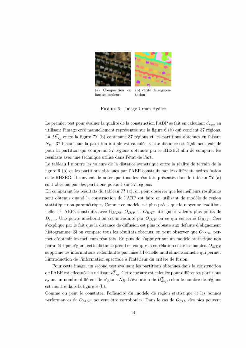
(a) Composition enfausses couleurs
(b) vérité de segmen-tation
Figure 6 – Image Urban Hydice
Le premier test pour évaluer la qualité de la construction l’ABP se fait en calculant dsym en
utilisant l’image créé manuellement représentée sur la figure 6 (b) qui contient 37 régions.
La DTasy entre la figure ?? (b) contenant 37 régions et les partitions obtenues en faisant
Np - 37 fusions sur la partition initiale est calculée. Cette distance est également calculé
pour la partition qui comprend 37 régions obtenues par le RHSEG afin de comparer les
résultats avec une technique utilisé dans l’état de l’art.
Le tableau I montre les valeurs de la distance symétrique entre la réalité de terrain de la
figure 6 (b) et les partitions obtenues par l’ABP construit par les différents ordres fusion
et le RHSEG. Il convient de noter que tous les résultats présentés dans le tableau ?? (a)
sont obtenus par des partitions portant sur 37 régions.
En comparant les résultats du tableau ?? (a), on peut observer que les meilleurs résultants
sont obtenus quand la construction de l’ABP est faite en utilisant de modèle de région
statistique non paramétriques.Comme ce modèle est plus précis que la moyenne tradition-
nelle, les ABPs construits avec OMDS , ODIF et OBAT atteignent valeurs plus petits de
Dsym. Une petite amélioration est introduite par ODIF en ce qui concerne OBAT . Ceci
s’explique par le fait que la distance de diffusion est plus robuste aux défauts d’alignement
histogramme. Si on compare tous les résultats obtenus, on peut observer que OMDS per-
met d’obtenir les meilleurs résultats. En plus de s’appuyer sur un modèle statistique non
paramétrique région, cette distance prend en compte la corrélation entre les bandes. OMDS
supprime les informations redondantes par mise à l’échelle multidimensionnelle qui permet
l’introduction de l’information spectrale à l’intérieur du critère de fusion.
Pour cette image, un second test évaluant les partitions obtenues dans la construction
de l’ABP est effectuée en utilisant dTasy. Cette mesure est calculée pour différentes partitions
ayant un nombre différent de régions NR. L’évolution de DTasy, selon le nombre de régions
est montré dans la figure 8 (b).
Comme on peut le constater, l’efficacité du modèle de région statistique et les bonnes
performances de OMDS peuvent être corroborées. Dans le cas de OSID des pics peuvent
14
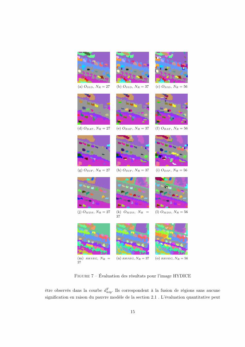
(a) OSID, NR = 27 (b) OSID, NR = 37 (c) OSID, NR = 56
(d) OBAT , NR = 27 (e) OBAT , NR = 37 (f) OBAT , NR = 56
(g) ODIF , NR = 27 (h) ODIF , NR = 37 (i) ODIF , NR = 56
(j) OMDS , NR = 27 (k) OMDS , NR =
37
(l) OMDS , NR = 56
(m) RHSEG, NR =27
(n) RHSEG, NR = 37 (o) RHSEG, NR = 56
Figure 7 – Évaluation des résultats pour l’image HYDICE
être observés dans la courbe dTasy. Ils correspondent à la fusion de régions sans aucune
signification en raison du pauvre modèle de la section 2.1 . L’évaluation quantitative peut
15
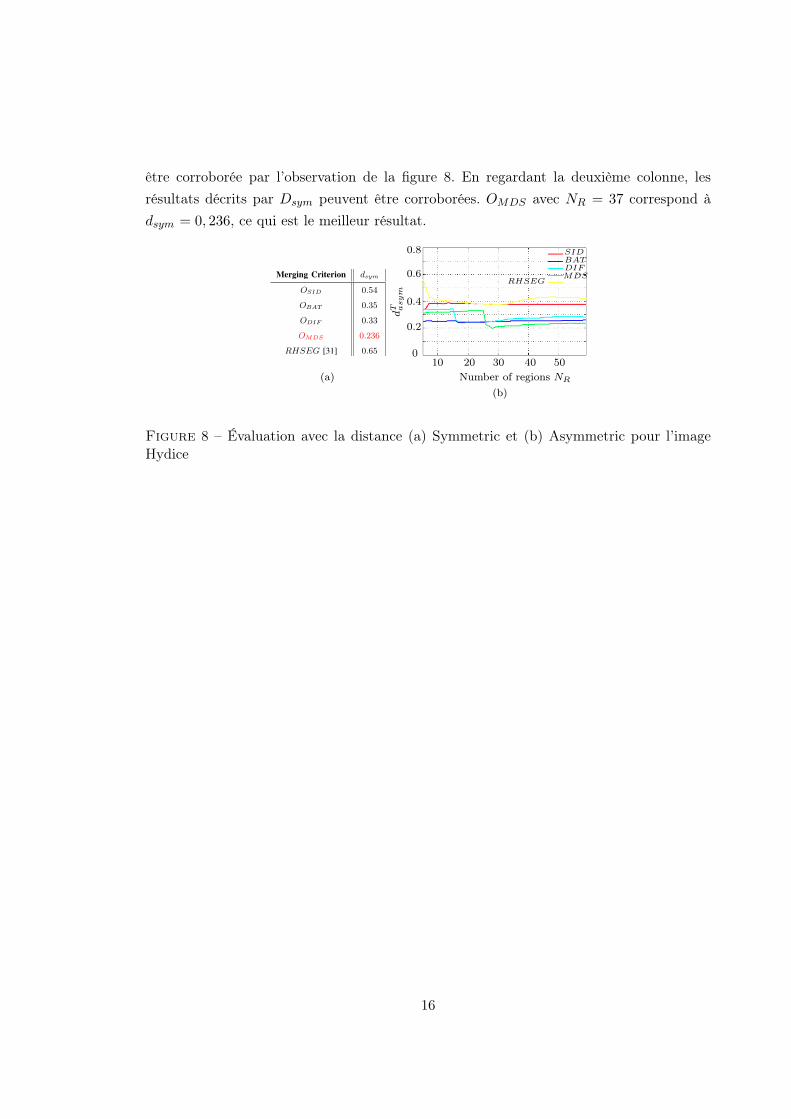
être corroborée par l’observation de la figure 8. En regardant la deuxième colonne, les
résultats décrits par Dsym peuvent être corroborées. OMDS avec NR = 37 correspond à
dsym = 0, 236, ce qui est le meilleur résultat.
Merging Criterion dsym
OSID 0.54
OBAT 0.35
ODIF 0.33
OMDS 0.236
RHSEG [31] 0.65
dT asym
Number of regions NR
(b)
(a)
0
0.2
0.4
0.6
0.8
10 20 30 40 50
SIDBATDIFMDS
RHSEG
Figure 8 – Évaluation avec la distance (a) Symmetric et (b) Asymmetric pour l’imageHydice
16
4 L’élagage de l ’ABP
4.1 La classification supervisée
La classification supervisée des images hyperspectrales en utilisant l’ABP consiste à
supprimer les sous-arbres composés de nœuds appartenant à la même classe. Ainsi, l’ob-
jectif final est d’utiliser l’ABP élagué pour construire une carte de classification complète
de l’image. Cela est possible en sélectionnant les feuilles de l’ABP élagué. La méthode
proposée dans cette thèse se compose de deux étapes différentes. Tout d’abord, certains
descripteurs spécifiques à chaque région sont calculés pour chaque nœud de l’ABP. Puis, la
deuxième étape implique une analyse des branches de l’ABP afin de prendre une décision
sur l’élagage.
4.1.1 Calcul des descripteurs
Dans la classification supervisée au niveau du pixel [4], des échantillons connus sont
utilisés pour spécifier les attributs spectrales des différentes classes composant la scène.
Ensuite, un algorithme de classification compare les pixels de l’image avec les caractéris-
tiques spectrales de chaque classe pour décider l’appartenance à la classe la plus probable.
L’inconvénient de cette approche est sa manque de robustesse. Cela est du au fait que cette
approche est uniquement basée sur l’information spectrale des pixels. Par conséquent, la
corrélation spatiale dans l’image n’est pas prise en compte. Dans ce contexte, l’avantage de
l’utilisation de l’ABP vient du fait que la corrélation spatiale des pixels a déjà été exploitée
lors de la construction de l’ABP. En fait, cette représentation correspond à un ensemble
de régions contenues dans une structure hiérarchique, lesquelles peuvent être classés en
fonction de leur spectre moyen.
Dans ce travail, le Support Vector Machine (SVM) [2] est utilisé a titre d’exemple. Suivant
l’approche classique, l’entrainement de ce classifieur est fait par un ensemble de pixels pour
lesquels la vérité de terrain est connu. Ensuite, ce classifier est utilisé pour calculer une
descripteur spécifique pour tous les noeuds de l’ABP. Ce descripteur, sur lequel l’élagage
présenté ici est basé, correspond à la distribution de probabilité des différentes classes ap-
partenant a la vérité de terrain. Autrement dit, chaque nœud Ri de l’ABP est représentée
par son spectre moyen et le SVM est ensuite utilisé pour estimer la probabilité que ce
spectre a pour toutes les classes possibles Cj . La distribution des classes qui en résulte est
notée par PRi(Cj) et elles sont estimées par [17] . Une fois que la distribution de probabilité
a été calculé pour chaque nœud, le taux de classification erroné est calculé. Pour les nœuds
feuilles, elle correspond à l’erreur commise lors de la classe la plus probable est attribuée
au noeud. Il est défini par :
17
MR(Ri) = (1−Maxj
PRi(Cj)) (18)
Pour les nœuds qui ne sont pas de feuilles, cette expression n’est pas appropriée. Par
exemple, si une région résulte de la fusion d’une grande région avec une petite région, la
petite région a peu d’influence sur le spectre moyen, même si sa classe est différente de la
classe de la grande région. Pour contourner ces limitations, le taux d’erreur de classification
d’une région peut être estimée par la mesure de similarité entre les deux distributions de
classes des deux noeuds qui vont se fusionner. Ici, le classique Bhattacharyya Coefficient
est utilisé pour mesurer la similarité entre les distributions comme :
BC(PLRi,PR
Ri) =
X
j
q
PLRi(Cj)PR
Ri(Ci) (19)
ou PLRi
and PRRi
représentent respectivement la distribution de probabilités des enfants
gauche et droite de la région Ri. En utilisant cette mesure, le taux d’erreur de classification
pour les régions non feuilles est défini par :
MR(Ri) = (1− BC(PLRi,PR
Ri)) (20)
4.1.2 L’analyse des branches
Une fois que le taux d’erreur de classification a été calculé pour tous les nœuds, une
décision doit être prise afin de décider l’élagage de l’arbre. Pour ce but-là, nous étudions
l’évolution du taux d’erreur de classification entre les noeuds Ri et ses feuilles Rfeuillesi ,
(c’est à dire les feuilles qui appartiennent à la sous-arborescence dont la racine est Ri).
Plus précisément, la décision d’élagage est définie par :
φR(Ri) = MR(Ri)−MR(Rleavesi ) (21)
ou MR(Rleavesi ) représente le taux d’erreur de classification moyenne des feuilles de Ri.
Notez que cette règle n’est pas croissante. Ainsi, nous utilisons ici la décision maximale,
c’est à dire, une stratégie ascendante qui consiste à élager tous les nœuds pour lesquels
MR(Ri) est inférieur à un seuil αC et telle que cette affirmation est également vraie pour
tous leurs descendants. Les évaluations expérimentales ont montrée que une valeur αC
environ 0,3 est appropriée. Enfin, une fois que l’arbre a été élagué, la carte de classification
est réalisée en attribuant la classe la plus probable (tel que défini par la SVM) aux régions
contenues dans les feuilles de l’arbre élagué.
Un exemple de classification est montré ici en utilisant les données hyperspectral AVIRIS
18

Indian Pines aient 200 bandes spectrales. Une composition RGB de ce jeu de données est
représentée sur la figure. 9. Dans cette figure, la vérité de terrain composée de 16 classes
différentes est aussi illustrée. Pour cette image, deux ABPs ont été créés, l’un en utilisant
la distance de diffusion, ODIF et un autre en utilisant le critère OMDS décrite au 2.2.3.
Dans les deux cas, les modèles de régions en utilisant les histogrammes sont construits avec
NBins=150.
!! ! !!!!"#$ $ $ $
(a) Composition couleur (b) Vérité de terrain
Figure 9 – Données hyperspectral AVIRIS Indian Pines
Les deux cartes de classification obtenues après l’élagage des deux ABPs sont présen-
tées dans la figure 10. Cette dernière figure montrée aussi le résultat obtenue en utilisant
l’approche classique au niveau de pixel (résultat obtenu avec le même classifieur SVM).
Comme on peut constater, l’approche ABP donne de bien meilleurs résultats que l’ap-
proche classification pixel par pixel. L’élagage de l’ABP obtient des cartes de classification
ou les régions sont moins bruyantes et la qualité des contours est très bonne.
(a) Classif. niveau pixel (b) ABP, ODIF (c) ABP, OMDS
Figure 10 – Cartes de classifications
L’évaluation quantitative de ces résultats est illustrée dans le tableau 1. La meilleure
de résultats obtenus grâce à l’ABP est tout à fait clair. D’autre part, on peut conclure que
19
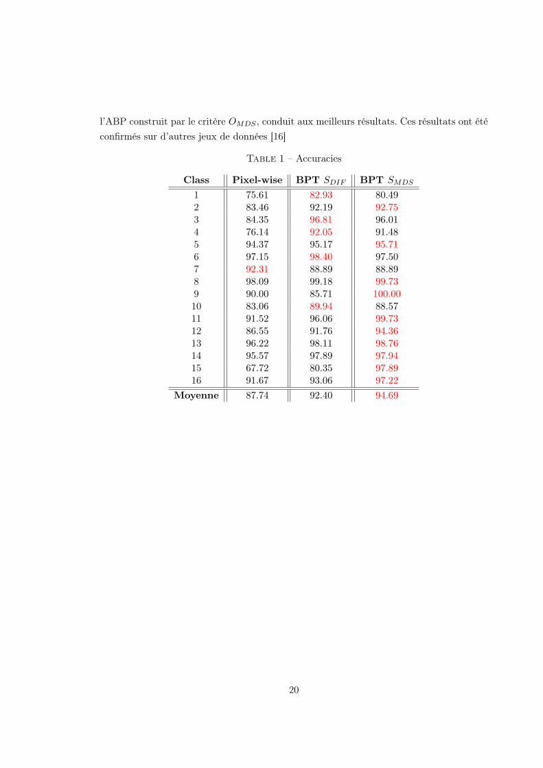
l’ABP construit par le critère OMDS , conduit aux meilleurs résultats. Ces résultats ont été
confirmés sur d’autres jeux de données [16]
Table 1 – Accuracies
Class Pixel-wise BPT SDIF BPT SMDS
1 75.61 82.93 80.492 83.46 92.19 92.753 84.35 96.81 96.014 76.14 92.05 91.485 94.37 95.17 95.716 97.15 98.40 97.507 92.31 88.89 88.898 98.09 99.18 99.739 90.00 85.71 100.0010 83.06 89.94 88.5711 91.52 96.06 99.7312 86.55 91.76 94.3613 96.22 98.11 98.7614 95.57 97.89 97.9415 67.72 80.35 97.8916 91.67 93.06 97.22
Moyenne 87.74 92.40 94.69
20
4.2 La segmentation supervisée
La deuxième application étudiée dans cette thèse est la segmentation non supervisée
des images hyperspectrales. Cela consiste à extraire de l’ABP une partition de l’image for-
mée par les régions les plus significatives. Cette tâche consiste à supprimer les sous-arbres
qui peuvent être remplacés par un seul nœud. Cela est possible si tous les noeuds à l’in-
térieur d’un sous-arbre appartiennent à la même région dans l’image. Cela signifie que la
distance entre eux est faible et la distance entre eux et leurs noeuds voisins est élevé. Dans
ce contexte, une technique de segmentation réalisant l’élagage de l’ABP a été proposée
dans ce thèse. Cette technique est basée sur la réalisation des coupes normalisées sur les
branches de l’ABP. Pour cela, des techniques classiques de partitionnement de graphes ont
été étudiées.
Les algorithmes de partitionemment de graphes sont très connus dans le traitement des
images. Ces approches peuvent potentiellement être utilisé sur l’ABP car il est en fait une
graphe binaire. Dans ce travail, nous nous concentrons sur l’algorithme de coupe norma-
lisée décrit dans [9]. Cette approche repose sur un graphe générique G formée par NN
nœuds, dont chaque branche entre les nœuds i et j est pondérée par une poids wi,j . Le
partitionnement optimal de ce graphe pondéré donne lieu à deux sous-ensembles de nœuds,
U et V , de telle sorte que le coût qu’on cherche a minimisé est le suivant :
Ncut(U ,V) =cut(U ,V)
assoc(U ,NN )+
cut(U ,V)
assoc(V,NN )(22)
ou cut(U ,V) =P
i∈U , j∈V wij and assoc(U ,NN ) =P
i∈U , j∈NNwij .
Ce problème de minimisation peut être formulé comme un problème dans la théorie spec-
trale des graphes [9] lequel peut être résolu en trouvant les vecteurs propres de (D−W)x =
λDx, ou W = [wi,j ] est la matrice d’affinité et D est une matrice diagonale dont les élé-
ments diagonaux sont di =P
∀j wij . Ainsi, le signe des composantes du vecteur propre
associé au deuxième plus petit valeur propre est utilisé pour créer une partition du graphe
qui minimise le cout normalisé donnée par l’équation 22.
Nous utilisons cette méthode de coupe normalisée pour la partition individuel de chaque
branche de l’ABP. Dans notre cas, une branche est défini comme un trajet qui relie le
noeud racine de l’ABP, RRacine, à une de ses noeud feuille, Rfeuille. De cette façon, une
branche représente un graphe très simple avec une structure linéaire ou la stratégie de la
coupe normalisée peut être effectuée. Dans la partie de la branche qui doit être élagué
les nœuds devront être similaires au nœud feuille. En revanche, les nœuds qui vont être
préservés devrait être les noeuds différents du nœud feuille. Si P (Ri = Rfeuille) désigne la
probabilité que Ri est semblable à la feuille Rfeuille, le poids wij associé a chaque branche
21
est alors défini par :
e√
P (Ri=Rfeuille)P (Rj=Rfeuille)+√
P (Ri 6=Rfeuille)P (Rj 6=Rfeuille)−1
Ce poids devrait indiquer que les nœuds formant les deux ensembles de la coupe résul-
tant sont très similaires (parce qu’ils sont très proches ou très dissemblable de la feuille).
Plusieurs solutions peuvent être utilisées pour estimer P (Ri = Rfeuille). Dans cet étude, le
critère MDS : P (Ri = Rfeuille) = OMDS(Ri, Rfeuille) définie pour la construction de l’ABP
a été utilisé. Afin de construire la matrice d’affinité, les poids wi,j ne sont pas calculés entre
tous les nœuds de la branche, mais seulement entre un noeud et ses deux enfants, son frère
et son ancêtre direct.
Dans la pratique, la première coupe peut-être pas la meilleure. Par exemple, si le nœud
racine est très différente de la reste de l’arbre, la première coupe va séparer, pour toutes
les branches, la racine du reste de la branche. Pour cette raison, au lieu d’une seule coupe,
un algorithme récursif spectrale de partitionnement de graphe est effectuée comme suggéré
dans [9]. L’idée est de parcourir le partitionnement de la branche sur le sous-ensemble de
noeuds qui inclut le Rfeuille jusqu’à la valeur Ncut est inférieure à un seuil TNcut (réglé
sur 0.3 pour toutes les expériences).
Une fois que chaque branche a été étudiée avec l’algorithme de coupe normalisée, l’élagage
doit être effectuée. Pour cela, les informations provenant de les partitions individuelles de
chaque branche doivent être fusionnés. En fait, à l’exception des noeuds feuilles, chaque
nœud d’ABP appartient à plusieurs branches. Ainsi, pour savoir si un nœud doit être éla-
gués ou non, un vote majorité est réalisée sur la base des résultats de toutes les branches :
Si un nœud appartient à M branches différentes et plus de M/2 branches ont déclaré que
le noeud doit être élagué, il sera élagué. Enfin, comme dans le cas de l’élagage effectué
par la classification, la décision d’élagage n’est pas croissante. Comme dans le cas de la
classification, cet effet a été traité de sorte qu’un nœud est élagué seulement si tous ses
descendants doivent également être élagués.
La figure 11 montrée les résultats obtenus par l’approche de segmentation présentée ici
pour quatre images hyperspectrales. La figure 11(a) et 11(b) ont été extraites à partir des
données Université de Pavia qui a été acquise sur la ville de Pavie (Italie) par le capteur
hyperspectral ROSIS-03 (Optique réfléchissantes Systèmes Imaging Spectrometer). La ré-
solution spatiale est de 1.3m. Ces données sont composées de 103 bandes spectrales allant
de 0.43 to 0.86µm m avec une bande passante de 4nm. La figure 11(c) acquise aussi par le
capteur hyperspectrale ROSIS-03 correspond au centre ville de Pavia. Cette image contient
102 bandes spectrales après le retrait des bandes bruyantes. Enfin, la figure 11(d) a été
22
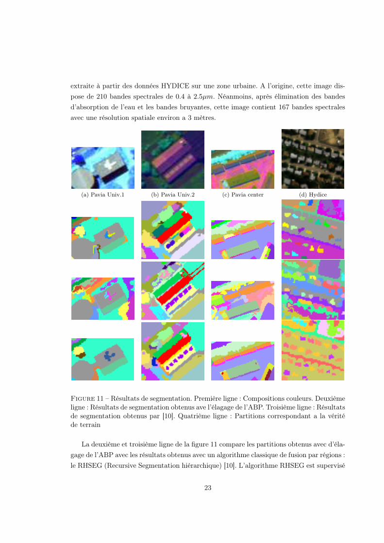
extraite à partir des données HYDICE sur une zone urbaine. A l’origine, cette image dis-
pose de 210 bandes spectrales de 0.4 à 2.5µm. Néanmoins, après élimination des bandes
d’absorption de l’eau et les bandes bruyantes, cette image contient 167 bandes spectrales
avec une résolution spatiale environ a 3 mètres.
(a) Pavia Univ.1 (b) Pavia Univ.2 (c) Pavia center (d) Hydice
Figure 11 – Résultats de segmentation. Première ligne : Compositions couleurs. Deuxièmeligne : Résultats de segmentation obtenus ave l’élagage de l’ABP. Troisième ligne : Résultatsde segmentation obtenus par [10]. Quatrième ligne : Partitions correspondant a la véritéde terrain
La deuxième et troisième ligne de la figure 11 compare les partitions obtenus avec d’éla-
gage de l’ABP avec les résultats obtenus avec un algorithme classique de fusion par régions :
le RHSEG (Recursive Segmentation hiérarchique) [10]. L’algorithme RHSEG est supervisé
23
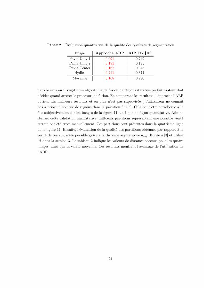
Table 2 – Évaluation quantitative de la qualité des résultats de segmentation
Image Approche ABP RHSEG [10]
Pavia Univ.1 0.091 0.249Pavia Univ.2 0.191 0.193Pavia Center 0.167 0.345
Hydice 0.211 0.374
Moyenne 0.165 0.290
dans le sens où il s’agit d’un algorithme de fusion de régions itérative ou l’utilisateur doit
décider quand arrêter le processus de fusion. En comparant les résultats, l’approche l’ABP
obtient des meilleurs résultats et en plus n’est pas supervisée ( l’utilisateur ne connait
pas a priori le nombre de régions dans la partition finale). Cela peut être corroborée à la
fois subjectivement sur les images de la figure 11 ainsi que de façon quantitative. Afin de
réaliser cette validation quantitative, différents partitions représentant une possible vérité
terrain ont été créés manuellement. Ces partitions sont présentés dans la quatrième ligne
de la figure 11. Ensuite, l’évaluation de la qualité des partitions obtenues par rapport à la
vérité de terrain, a été possible grâce à la distance asymétrique dasy décrite à [3] et utilisé
ici dans la section 3. Le tableau 2 indique les valeurs de distance obtenus pour les quatre
images, ainsi que la valeur moyenne. Ces résultats montrent l’avantage de l’utilisation de
l’ABP.
24
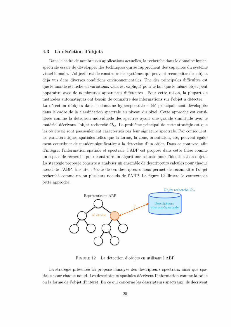
4.3 La détéction d’objets
Dans le cadre de nombreuses applications actuelles, la recherche dans le domaine hyper-
spectrale essaie de développer des techniques qui se rapprochent des capacités du système
visuel humain. L’objectif est de construire des systèmes qui peuvent reconnaître des objets
déjà vus dans diverses conditions environnementales. Une des principales difficultés est
que le monde est riche en variations. Cela est expliqué pour le fait que le même objet peut
apparaître avec de nombreuses apparences différentes . Pour cette raison, la plupart de
méthodes automatiques ont besoin de connaitre des informations sur l’objet à détecter.
La détection d’objets dans le domaine hyperspectrale a été principalement développée
dans le cadre de la classification spectrale au niveau du pixel. Cette approche est consi-
dérée comme la détection individuelle des spectres ayant une grande similitude avec le
matériel décrivant l’objet recherché Ore. Le problème principal de cette stratégie est que
les objets ne sont pas seulement caractérisés par leur signature spectrale. Par conséquent,
les caractéristiques spatiales telles que la forme, la zone, orientation, etc, peuvent égale-
ment contribuer de manière significative à la détection d’un objet. Dans ce contexte, afin
d’intégrer l’information spatiale et spectrale, l’ABP est proposé dans cette thèse comme
un espace de recherche pour construire un algorithme robuste pour l’identification objets.
La stratégie proposée consiste à analyser un ensemble de descripteurs calculés pour chaque
nœud de l’ABP. Ensuite, l’étude de ces descripteurs nous permet de reconnaître l’objet
recherché comme un ou plusieurs noeuds de l’ABP. La figure 12 illustre le contexte de
cette approche.
Objet recherché Ore
DescripteursSpatiale-Spectrale?
Représentation ABP
N étudié
Figure 12 – La détection d’objets en utilisant l’ABP
La stratégie présentée ici propose l’analyse des descripteurs spectraux ainsi que spa-
tiales pour chaque nœud. Les descripteurs spatiales décrivent l’information comme la taille
ou la forme de l’objet d’intérêt. En ce qui concerne les descripteurs spectraux, ils décrivent
25

les spectres des régions. Par exemple, si le matériau de l’objet Ore est connue, la signa-
ture spectrale est alors une importante descripteur du matériau. La technique d’élagage
proposée ici repose sur trois descripteurs différents calculés pour tous les nœuds de l’ABP
O = Dforme, Dspectrale, Dtaille (23)
Le calcul de l’ensemble des descripteurs pour tous les nœuds est la première étape dans
la technique de élagage adaptée la détection d’objets. Ainsi, une fois que les descripteurs
proposés D sont calculés, ils sont étudiés suivant une approche ascendante depuis les feuilles
à la racine. L’approche consiste à élaguer tous les noeuds qui sont différents de l’objet
de référence Ore. Pour cela, la stratégie consiste à considérer que les objets recherchés
correspond aux nœuds les plus proches au racine qui ont un ensemble de descripteurs
similaire à Ore. Afin d’illustrer la généralité de l’approche, deux exemples de détection
d’objets dans des scènes urbaines sont présentés ici : la détection de routes et la détection
des bâtiments .
4.3.1 La détection de routes
Les routes apparaissent comme des structures allongées avec des valeurs de radiance
généralement assez homogènes correspondant à la classe asphalte. En conséquence, dans
une classification classique pixel par pixel, la détection des routes consiste clairement à
la détection des pixels de l’image qui appartiennent à la classe d’asphalte. Le principal
inconvénient de cette approche est que d’autres structures de l’image peut également être
formé par de l’asphalte. Pour résoudre ce problème, l’inclusion de l’information spatiale
est primordial. Ainsi, prenant en compte la forme des routes, l’élongation de la région est
utilisée ici comme le descripteur de forme Dforme. Cela peut être calculée avec la relation
des axes concernant la plus petite bounding box orientée contenant la région (rapport entre
la largeur et la hauteur de la bounding box).
Le deuxième descripteur spatiale calculée aux nœuds de l’ABP est la taille de région Dtaille.
Le but est de supposer que la route devrait avoir au moins un nombre minimum de pixels.
Cette taille minimale requise devrait être fixé en fonction de la résolution spatiale de
l’image. Concernant le descripteur spectral Dspectrale, il doit contenir l’information décri-
vant si le noeud de l’ABP appartient a la classe l’asphalte. Ainsi, compte tenu d’un spectre
de référence de la classe asphalte, le coefficient de corrélation entre le spectre moyen du
noeud de l’ABP et un spectre de référence de la classe asphalte est utilisée comme Dspectrale.
Ce coefficient peut être calculé par l’équation 24 où INλ est le spectre moyen contenu dans
N .
26
Dspectrale(N ) =
NzX
z=1
(INλz−
1
Nz
NzX
s=1
INλs)(IOre
λz−
1
Nz
NzX
s=1
IOre
λs)
v
u
u
t
NzX
z=1
(INλz−
1
Nz
NzX
s=1
INλs)2
v
u
u
t
NzX
z=1
(IOre
λz−
1
Nz
NzX
s=1
IOre
λs)2
(24)
Après le calcul des trois descripteurs formant O pour tous les nœuds de l’ABP, l’idée
est de sélectionner les nœuds les plus proches de la racine, qui ont une petite élongation,
une forte corrélation avec la classe asphalte et une taille supérieure à un seuil fixé.
4.3.2 La détection des bâtiments
La détection des bâtiments suivi la même stratégie présentée ci-dessus pour les routes.
Ainsi, trois descripteurs sont également définies. Concernant le descripteur Dspectrale, ce
coefficient correspond également à un coefficient de corrélation entre le spectre moyenne de
chaque noeud de l’ABP et un spectre de référence. Dans le cas de la taille, le descripteur
Dtaille est également défini selon la taille qui ont les bâtiments dans l’image.
La principale différence avec l’exemple de la détection de routes vient du fait que l’élon-
gation de la région Dforme n’est pas appropriée dans le cas de bâtiments. Par conséquent,
un autre descripteur de forme est utilisé dans le cas des bâtiments. L’idée est d’utiliser
la rectangularité d’une région comme Dforme . Le calcul de ce descripteur spatial peut
être facilement réalisée avec la définition de la bounding box orientée . Ainsi, Dforme est
calculée comme le rapport de la taille de la région contenue dans le noeud et la surface de
la bounding box. Théoriquement, une zone rectangulaire va avoir une valeur similaire au
Dforme = 1 (le cas égalité est pour les régions parfaitement rectangulaires).
Ensuite, suivant la même stratégie que pour le cas de la réseau routière, une analyse des-
cendante de recherche dans l’arbre est réalisée afin d’extraire les les nœuds plus proches
de la racine similaires au Ore.
Dans la suite, la stratégie de détection d’objets pour la détection des routes et bâtiments
en utilisant l’ABP est évaluée ici. Le but de ces expériences est de comparer les résultats
obtenues en utilisant l’ABP avec une classification classique pixel par pixel. Ces expériences
ont été effectuées avec la portion de l’image hyperspectrale HYDICE utilisée dans la sec-
tion précédente. La figure 13(a) montrée une combinaison couleur de la portion d’image.
L’ABP a été calculée en utilisant le critère OMDS . Les vérités de terrain de cette image
illustrant les routes et les bâtiments de la scène sont présentées sur les figure 13(b) et 13(c).
La classification au niveau de pixel consiste à détecter les pixels de l’image aient une
corrélation supérieure à 0,9 avec le spectre de référence. Pour détecter les Ore des pa-
ramètres de référence doit être défini. Par exemple, dans le cas des routes, la stratégie
27
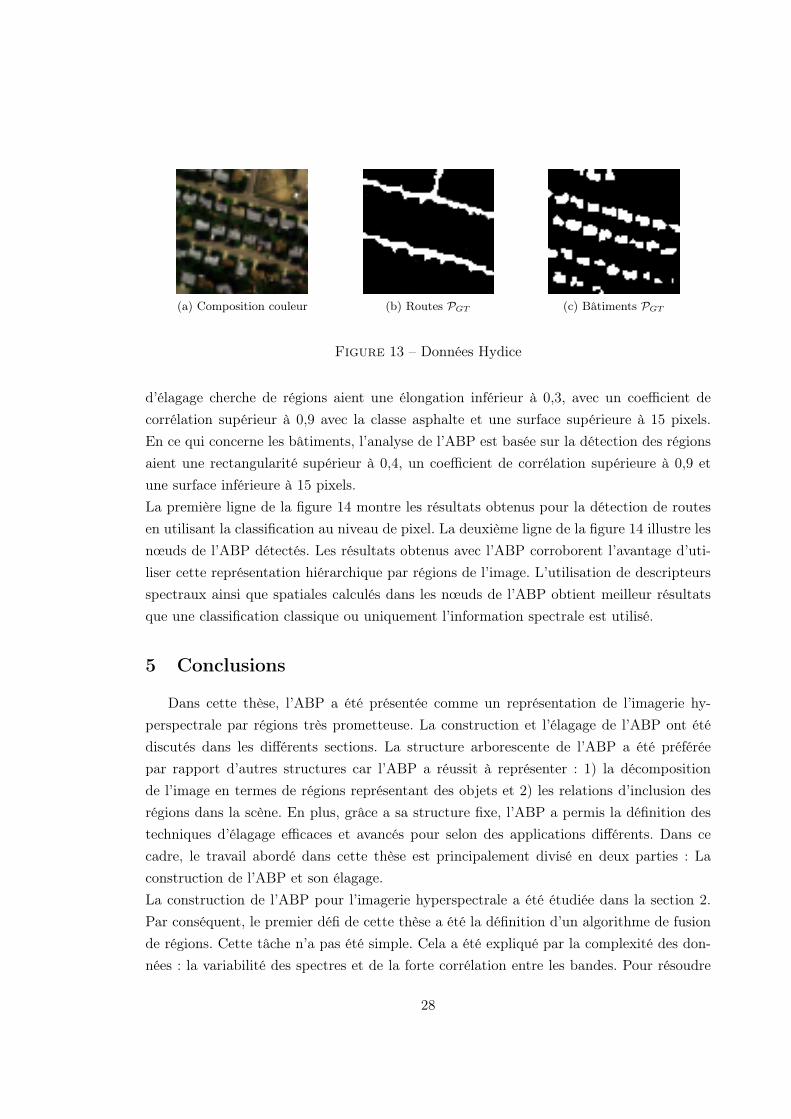
(a) Composition couleur (b) Routes PGT (c) Bâtiments PGT
Figure 13 – Données Hydice
d’élagage cherche de régions aient une élongation inférieur à 0,3, avec un coefficient de
corrélation supérieur à 0,9 avec la classe asphalte et une surface supérieure à 15 pixels.
En ce qui concerne les bâtiments, l’analyse de l’ABP est basée sur la détection des régions
aient une rectangularité supérieur à 0,4, un coefficient de corrélation supérieure à 0,9 et
une surface inférieure à 15 pixels.
La première ligne de la figure 14 montre les résultats obtenus pour la détection de routes
en utilisant la classification au niveau de pixel. La deuxième ligne de la figure 14 illustre les
nœuds de l’ABP détectés. Les résultats obtenus avec l’ABP corroborent l’avantage d’uti-
liser cette représentation hiérarchique par régions de l’image. L’utilisation de descripteurs
spectraux ainsi que spatiales calculés dans les nœuds de l’ABP obtient meilleur résultats
que une classification classique ou uniquement l’information spectrale est utilisé.
5 Conclusions
Dans cette thèse, l’ABP a été présentée comme un représentation de l’imagerie hy-
perspectrale par régions très prometteuse. La construction et l’élagage de l’ABP ont été
discutés dans les différents sections. La structure arborescente de l’ABP a été préférée
par rapport d’autres structures car l’ABP a réussit à représenter : 1) la décomposition
de l’image en termes de régions représentant des objets et 2) les relations d’inclusion des
régions dans la scène. En plus, grâce a sa structure fixe, l’ABP a permis la définition des
techniques d’élagage efficaces et avancés pour selon des applications différents. Dans ce
cadre, le travail abordé dans cette thèse est principalement divisé en deux parties : La
construction de l’ABP et son élagage.
La construction de l’ABP pour l’imagerie hyperspectrale a été étudiée dans la section 2.
Par conséquent, le premier défi de cette thèse a été la définition d’un algorithme de fusion
de régions. Cette tâche n’a pas été simple. Cela a été expliqué par la complexité des don-
nées : la variabilité des spectres et de la forte corrélation entre les bandes. Pour résoudre
28

(a) (b)
(c) (d)
Figure 14 – Première ligne : Détection au niveau de pixel des routes (a) et bâtiments (b).Deuxième ligne : Détection en utilisant l’ABP des routes (c) et bâtiments (d)
ces problèmes, plusieurs modèles des régions et des mesures de similarité ont été étudiées
[14]. Concernant les modèles de la région, le modèle plus utilisé dans la littérature décrit
ici comme le modèle du premier ordre a été comparé avec le modèle statistique non para-
métrique précédemment définie dans [1] pour l’imagerie classique. L’utilisation du modèle
de région non paramétrique statistique a été proposé comme une solution pour représenter
un ensemble de spectres. Ce modèle de région a montré ses performances concernant le
problème de la variabilité spectrale. En outre, il a prouvé ses capacités à représenter les
régions complexes ou texturées. Selon le modèle de région statistique non paramétrique,
différents critères de fusion ont été proposées. Le problème lié à la distance Battacharyya
décrit dans [1] a été résolu en utilisant la distance de diffusion. L’utilisation d’une distance
inter-bin a confirmé son avantage montrant sa robustesse au paramètre Nbins. Malgré des
résultats intéressants fournis par cette distance, la question de corrélation n’a pas été abor-
dée dans ce cas.
Par conséquent, un nouveau critère de fusion prenant en compte la corrélation entre les
bandes hyperspectrales a été proposé comme une des principales contributions de la thèse
à la section 2.2.3. L’idée a été de réduire localement la dimension de la région hyperspectral
en utilisant le MDS. Les coordonnées principales locales de chaque région ont été extraites
par l’étude des similitudes entre les histogrammes représentant la région. Ensuite, un test
statistique basé sur la théorie MANOVA a été proposé pour mesurer la similarité entre
deux régions adjacentes. Ce test a été également liée aux corrélations canoniques. Dans ce
29
contexte, une estimation du choix de la dimension pour comparer les coordonnées princi-
pales des deux régions a été présenté dans ce travail.
Les différents ordres de fusion ont été évalués en étudiant les partitions obtenues lors de
la construction de l’ABP. Une évaluation visuel et quantitative a été réalisées afin d’éva-
luer les résultats. L’évaluation quantitative a été effectuée avec les distance symétrique et
asymétriques présentés à la section 3. A notre connaissance, cette thèse a mis en place la
première évaluation quantitative permettant de valider la segmentation d’une image hy-
perspectrales concernant la totalité de l’image. Les résultats expérimentaux ont montrés
les bonnes performances de la construction de l’ABP en comparaison avec l’état de l’art
[13]. Les résultats obtenus ont également montrés les limitations du modèle de région de
premier ordre. En revanche, le critère de la fusion MDS a obtenu les meilleurs résultats
dans notre étude. Ainsi, ce critère de fusion peut être considérée comme une prometteuse
mesure pour mesurer les similitudes entre les ensembles de données hyperspectrales dans
des futurs travaux.
La deuxième contribution importante présentée dans cette thèse est la définition des dif-
férentes techniques d’élagage de l’ABP qui ont été présentées selon des applications dif-
férentes. Ces stratégies ont été proposés dans le contexte de la classification d images
hyperspectrales, la segmentation non supervisée et enfin, la détection d’objets. Le traite-
ment des images hyperspectrales en utilisant l’ABP a été présenté dans la section 4 comme
une stratégie d’élagage basée sur l’analyse des noeuds de l’arbre en mesurant un critère
spécifique. Les différentes stratégies ont corroborés la façon dont l’ABP n’est pas une repré-
sentation qui dépend d’une application. Néanmoins, elle est une représentation de l’image
qui peut être traitée par différentes stratégies d’élagages selon l’application.
Comme premier exemple, la classification supervisée des images hyperspectrales a été abor-
dée. Le classifieur SVM a été utilisé pour donner aux nœuds de l’ABP la distribution de
probabilité des classes. Ensuite, une analyse ascendante des branches a supprimé les nœuds
de l’ABP selon une règle de décision. Les résultats expérimentaux ont montrés que la mé-
thode proposée améliore la précision obtenu par un classifieur SVM classique. Les résultats
obtenus par l’ABP fournissant des cartes de classification moins de bruitées.
La deuxième stratégie d’élagage vise à attaquer la segmentation non supervisée d’images
hyperspectrales. À cette fin, une stratégie basée sur le coupe normalisée des branches de
l’ABP a été proposée. L’analyse des branches de l’ABP pour décider la meilleure coupe
a été adressée par l’interprétation des branches de l’ABP en tant que graphes réguliers
en incluant les connexions de nœuds frères. Ensuite, la théorie de graphes spectrale pour
partitioner une graphe a été appliqué pour obtenir des coupes normalisées. L’objectif a
été la partition de la branche en deux ensemble de données disjoints. En conséquence, le
partitionement de la branche doit être considéré comme un élagage local. Pour cela, les
30
coupes local des branches ont été utilisés ici pour donner aux nœuds de l’ABP un poids
décrivant quelle est la probabilité que ce nœud soit élagué. Ces poids ont été utilisés plus
tard pour effectuer une analyse ascendante de l’arbre selon un règle de décision. Cette règle
compare le poids d’un noeud avec sa taille pour décider si le noeud devrait être élagué.
Les résultats obtenus par cet élagage sont très positifs puisque utilisant les mêmes para-
mètres, il a été possible d’extraire des partitions avec le même nombre de régions que les
partitions de vérité de terrain. Les résultats ont montré comment une image hyperspec-
trale peut être divisée en régions cohérentes similaires aux régions appartenant à la vérité
de terrain. L’une des inconvénients de cet élagage vient du fait que l’étude des branches
est fait localement. Ainsi, l’application de la théorie des graphes spectrale complète pour-
rait être envisagée comme des futurs travaux de recherche. En plus, le calcul des matrices
d’affinité en utilisant l’ABP est une ligne de recherche encourageant. En effet, le calcul
de ces matrices a été fait principalement dans la littérature pour des structures classiques
comme le RAG. Par conséquent, l’idée d’utiliser une représentation d’image hiérarchique
par régions pourrait conduire à de meilleurs résultats.
Le dernière exemple d’élagage a été présenté dans le cadre de la détection d’objets. Deux
exemples ont été proposés afin d’illustrer l’intérêt de l’ABP dans le contexte de la re-
connaissance d’objets. Pour cela, la détection de routes et de bâtiments ont été proposés
comme exemples. La section 4.3 a décrit la façon dont l’information spectrale et spatiale
peut être incorporé dans la recherche d’un objet de référence. Ce travail peut être consi-
déré comme une contribution dans le domaine hyperspectrale. En effet, dans la plupart des
travaux rapportés dans la littérature, la détection d’objets a été uniquement abordé par le
classification au niveau pixel.
Références
[1] F. Calderero and F. Marques. “Region-merging Techniques Using Information Theory
Statistical Measures". In IEEE Transactions on Image Processing, vol.19(6), pp.1567-
1586, 2010.
[2] G. Camps-Valls and L. Bruzzone. Kernel-based methods for hyperspectral image classi-
fication. In IEEE Transactions on Geoscience and Remote Sensing, 43(6), pp.1351-1362,
2005.
[3] J.S. Cardoso and L. Corte-Real. “Toward a generic evaluation of image segmentation".
In IEEE Transactions on Image Processing, vol.14(11), pp.1773-1782, 2005.
[4] C.I. Chang. Hyperspectral Imaging : Techniques for Spectral Detection and Classifica-
tion. In Kluwer Academic Publishers, Dordrecht, 2003
31
[5] T.F. Cox and M.A. Cox. “Multidimensional Scaling", Chapman & Hall, London,1994.
[6] E. Cramer and W.A. Nicewander. “Some symmetric, invariant measures of multivariate
association." In Psychometrika, vol.44, pp-43-54, 1979.
[7] C.M. Cuadras, S. Valero, P. Salembier and J. Chanussot. “Some measures of multiva-
riate association relating two spectral data sets". In Proceedings of 19th International
Conference on Computational Statistics, Compstat, Paris, France, August 22-27 2010.
[8] C.M. Cuadras, A. Arenas and J. Fortiana. “Some computational aspects of a distance-
based model for prediction". in Communications in Statistics : Simulation and Com-
putation, vol.25, pp.593-609, 1996.
[9] J. Shi and J. Malik. “Normalized Cuts and Image Segmentation". In IEEE Transactions
on pattern analysis and machine intelligence, pp. 888-905, Vol. 22, No. 8, 2000.
[10] J.A. Gualtieri and J.C. Tilton, “Hierarchical Segmentation of Hyperspectral Data,"
2002 AVIRIS Earth Science and Applications Workshop, Pasadena, CA, March 5-8,
2002.
[11] H. Ling and K. Okada. “Diffusion distance for histogram comparison". In Proceedings
of IEEE Conference on Computer Vision and Pattern Recognition, CVPR, pp. 246-253,
New York, USA, 17-22 June 2006.
[12] P. Salembier and L. Garrido, “Binary partition tree as an efficient representation for
image processing, segmentation and information retrieval," in IEEE Transactions on
Image Processing, vol. 9(4), pp. 561-576, April 2000.
[13] J.Tilton. Image segmentation by region growing and spectral clustering with a natural
convergence criterion. In IEEE Proceedings of International Geoscience and Remote
Sensing Symposium (IGARSS), pp.1766-1768, 1998
[14] S. Valero, P. Salembier and J. Chanussot. “Comparison of merging orders and pruning
strategies for binary partition tree in hyperspectral data". in Proceedings of IEEE
International Conference of Image Processing, ICIP 10, pp. 2565 - 2568, Hong Kong,
China, September 2010.
[15] S. Valero, P. Salembier, J. Chanussot and C. Cuadras, “Improved Binary Parti-
tion Tree Construction for Hyperspectral Images : Application to Object Detection",
in Proceedings of IEEE International Geoscience and Remote Sensing Symposium,
IGARSS’2011, Vancouver, Canada, July 2011.
[16] S. Valero, P. Salembier and J. Chanussot, “Hyperspectral image representation and
processing with Binary Partition Trees", Accepted in IEEE Transactions on Image
Processing, 2012
32

[17] T.-F. Wu, C.-J. Lin, and R. C. Weng. “Probability estimates for multi-class classif-
fication by pairwise coupling”, Journal of Machine Learning Research, 5 :975 -1005,
2004.
33

Bibliography

164 BIBLIOGRAPHY
[1] A. Plaza, J.A. Benediktsson, J. Boardman, J. Brazile, L. Bruzzone, G. Camps-Valls, J. Chanus-
sot, M. Fauvel, P. Gamba, A. Gualtieri, J. Tilton and G. Trianni. Advanced Processing of Hy-
perspectral Images. In Remote Sensing of Environment, vol. 113, n 1, pp. S110-S122, 2009.
[2] C.I. Chang. Hyperspectral Imaging: Techniques for Spectral Detection and Classification. In
Kluwer Academic Publishers, Dordrecht, 2003
[3] D.A. Landgrebe. Signal Theory Methods in Multispectral Remote Sensing. In John Wiley and
Sons, 2003
[4] G. Camps-Valls and L. Bruzzone. Kernel-based methods for hyperspectral image classifica-
tion. In IEEE Transactions on Geoscience and Remote Sensing, 43(6), pp.1351-1362, 2005.
[5] L. Bruzzone, M. Chi, and M. Marconcini. A novel transductive SVM for semisupervised
classification remote sensing images. In IEEE Transactions on Geoscience and Remote Sensing,
vol.44(11), pp.3363-3373, 2006.
[6] M. Chi and L. Bruzzone. Semisupervised classification of hyperspectral images by SVMs opti-
mized in the primal. In IEEE Transactions on Geoscience and Remote Sensing, vol.45(6), pp.1870-
1880, 2007.
[7] C.-I Chang. Spectral information divergence for hyperspectral image analysis. in IEEE Pro-
ceedings of IGARSS, pp.509-511, Germany, 1999.
[8] A. Plaza, P. Martinez, R. Perez and J. Plaza. Spatial/spectral endmember extraction by multi-
dimensional morphological operations. in IEEE Transactions on Geoscience and Remote Sensing,
vol.40, pp.2025-2041, 2002.
[9] N. Gorretta, J.M Roger, G. Rabatel and V. Bellon-Maurel, C. Fiorio and C. Lelong. Hypersectral
image segmentation: The butterfly approach. In IEEE Proceedings of Workshop on Hyperspectral
Image and Signal Processing: Evolution in Remote Sensing, 2009.
[10] M. Fauvel, J.A. Benediktsson, J. Chanussot and J.R. Sveinsson. Spectral and Spatial Classifi-
cation of Hyperspectral Data Using SVMs and Morphological Profiles. In IEEE Transactions on
Geoscience and Remote Sensing, vol.46 (11), pp.3804-3814, 2008.
[11] A. Farag, R. Mohamed and A. El-Baz. A unified framework for map estimation in remote
sensing image segmentation. In IEEE Transactions on Geoscience and Remote Sensing, vol.43(7),
pp.1617-1634, 2005.
[12] J. Li, J. Bioucas-Dias and A. Plaza. Semi-Supervised Hyperspectral Image Segmentation Us-
ing Multinomial Logistic Regression with Active Learning. In IEEE Transactions on Geoscience
and Remote Sensing, vol.48(11), pp.4085-4098, 2010
[13] J. Angulo and S. Velasco-Forero. Semi-supervised hyperspectral image segmentation using
regionalized stochastic watershed. In Proceedings of the SPIE, vol.7695, 2010.
BIBLIOGRAPHY 165
[14] A. K. Jain, M. N. Murty, and P. J. Flynn. Data clustering: A review. In ACM Computing Surveys,
vol.31(3), pp.264-323, 1999.
[15] P. Salembier and L. Garrido. Binary partition tree as an efficient representation for image
processing, segmentation, and information retrieval. In IEEE Transactions on Image Processing,
vol.9(4), pp.561-576, 2000.
[16] F. Van der Meer. The effectiveness of spectral similarity measures for the analysis of hyper-
spectral imagery. In International Journal of applied earth observation and geoinformation, vol.8,
pp.3-17, 2006.
[17] F. Calderero, F. Marqués. Region-merging Techniques Using Information Theory Statistical
Measures. In IEEE Transactions on Image Processing, vol.19, pp.1567-1586, 2010.
[18] F. Calderero, F. Marques and A. Ortega. Performance Evaluation of Probability Density Esti-
mators for Unsupervised Information Theoretical Region Merging. In IEEE Proceedings of ICIP
2009, pp.4397-4400, Egypt, 2009
[19] S. Lee and M. Crawford. Unsupervised multistage image classification using hierarchi-
cal clustering with a Bayesian similarity measure. In IEEE Transactions on Image Processing,
vol.14(3), pp.312-320, 2005.
[20] Y. Tarabalka, J.A. Benediktsson, J. Chanussot. Spectral-Spatial Classification of Hyperspectral
Imagery Based on Partitional Clustering Techniques. In IEEE Transactions on Geoscience and
Remote Sensing, vol.47(8), pp.2973-2987, 2009.
[21] Y. Tarabalka, J. A. Benediktsson, J. Chanussot, and J. C. Tilton. Multiple Spectral–Spatial
Classification Approach for Hyperspectral Data. In IEEE Transactions on Geoscience and Remote
Sensing, vol. 48, no. 11, pp.4122-4132, 2010.
[22] J.A. Gualtieri and J. Tilton. Hierarchical Segmentation of Hyperspectral Data. In Proceedings
os AVIRIS Earth Science and Applications Workshop, pp.5-8, 2002.
[23] P. Coupe, P. Yger, S. Prima, P. Hellier, C. Kervrann, and C. Barillot. An Optimized Blockwise
Nonlocal Means Denoising Filter for 3-D Magnetic Resonance Images, In IEEE Transactions on
Medical Imaging, vol. 27(4), pp.425-441, 2008.
[24] M. Dimiccoli and P. Salembier. Hierarchical region-based representation for segmentation
and filtering with depth in single images. In IEEE Procedings of ICIP’09, pp.3533-3536, Egypt,
2009
[25] Y. Escoufier. Le Traitement des Variables Vectorielles. In Biometrics (International Biometric
Society) vol.29 (4): 751-76, 1973.
[26] C.M. Cuadras, S. Valero, P. Salembier and J. Chanussot. Some measures of multivariate asso-
ciation relating two spectral data sets. In Proceedings of Compstat 2010, France.
166 BIBLIOGRAPHY
[27] C.M. Cuadras. Multidimensional and Dependencies in Classification and Ordination. In K.
Fernandez and A. Morineau (Ed.), Analyses Multidimensionelle des Donnees, pp.15-25, France.
[28] T.F. Cox and M.A. Cox. Multidimensional Scaling. In K. Fernandez and A. Morineau
(Ed.),Chapman & Hal, London, 1994.
[29] T.W. Anderson. An Introduction to Multivariate Analysis. In Third Edition Wiley, New York,
2003.
[30] C.R. Rao, H. Toutenburg, A. Fieger, C. Heumann, T. Nittner and S. Scheid. Linear Models:
Least Squares and Alternatives. In Springer Series in Statistics, 1999
[31] E. Cramer and W.A. Nicewander. Some symmetric, invariant measures of multivariate asso-
ciation. In Psychometrika, vol.44, pp.43-54, 1979.
[32] J.C. Gower. Some distance properties of latent roots and vector methods used in multivariate
analysis in Biometrika , vol.53, pp.325-338, 1966.
[33] C.M. Cuadras, A. Arenas and J. Fortiana. Some computational aspects of a distance-based
model for prediction. In Communications in Statistics: Simulation and Computation , vol.25,
pp.593-609, 1996.
[34] M.H. Kutner, C.J. Nachtsheim, and J. Neter. Applied Linear Regression Model. In 4th ed.,
McGraw-Hill/Irwin, 2004.
[35] K.M. Rajpoot and N.M. Rajpoot. Wavelet based segmentation of hyperspectral colon tissue
imagery. In Proceedings 7th IEEE International Multitopic Conference INMIC, pp.38-43, 2003.
[36] I. Silverman, S.R. Rotman and C.E. Caefer. Segmentation of Hyperspectral Images from the
Histograms of Principal Components. In Imaging Spectrometry MII, Sylvia S. Shen , Editor, Pro-
ceedings of SPIE, vol.4816, 2002.
[37] G. Noyel, J. Angulo and D. Jeulin. Morphological segmentation of hyperspectral images. In
Image Anal. Stereol., vol.26, pp.101-109, 2007.
[38] M. Servais, T. Vlachos and T.Davies. Motion-compensation using variable-size block-
matching with binary partition trees. In IEEE Procedings of ICIP’05, vol.1, pp.I-157, Sept. 2005.
[39] V. Vilaplana, F. Marques and P. Salembier. Binary Partition Tree for Object Detection. in IEEE
Transactions on Image Processing, vol.17, pp.2201-2216, 2008.
[40] V. Vilaplana and F. Marques. On building a hierarchical region-based representation for
generic image analysis. In IEEE Proceedings of ICIP’07, vol.4, pp.325-328, 2007.
[41] T. Adamek and N.E. O’Connor. Using dempster-shafer theory to fuse multiple information
sources in region-based segmentation. In IEEE Proceedings of ICIP 2007, pp.269-272, 2007.
BIBLIOGRAPHY 167
[42] G. Scarpa, M. Haindl, and J. Zerubia. A hierarchical finite-state model for texture segmenta-
tion. In IEEE Proceedings of ICASSP ’07, vol.1, pp.1209-1212, 2007.
[43] Z. Liu, J. Yang and N. Peng. An efficient face segmentation algorithm based on binary parti-
tion tree. In Signal Processing Image Communication, vol.20(4), pp.295-314, 2005
[44] H. Lu, J.C. Woods and M. Ghanbari. Image segmentation by binary partition tree. In Elec-
tronics Letters, vol.42, pp.966-967, 2006
[45] S. Cooray, N. O’Connor, S. Marlow, N. Murphy and T. Curran. Semi-Automatic Video Object
Segmentation Using Recursive Shortest Spanning Tree and Binary Partition Tree. In Workshop
on Image Analysis for Multimedia Interactive Services, 2001.
[46] J. Pont-Tuset and F. Marques. Contour Detection using Binary Partition Trees. In IEEE Pro-
ceedings of ICIP’10, pp.1609-1612, 2010.
[47] C. Ferran Bennstrom and J. R. Casas. Binary partition tree creation using a quasi-inclusion
criterion. In Proceedings of 8th International Conference on Information Visualization, 2004.
[48] T. Adamek, Noel E. N. O’Connor, and Noel Murphy. Region-based segmentation of images
using syntactic visual features. In in Proceedins of 6th International Workshop on Image Analysis
for Multimedia Interactive Services, 2005.
[49] H. Lu, J. C. Woods, and M. Ghanbari. Binary Partition Tree for Semantic Object Extraction
and Image Segmentation. In IEEE Transactions on Circuits and Systems for Video Technology,
vol.17(3), pp.378-383, 2007.
[50] L. Breiman, J. Friedman, R. Olshen and C. Stone. Classification and Regression Trees. In
Wadsworth International Group, Belmont, CA.
[51] J.S. Cardoso and L. Corte-Real. Toward a generic evaluation of image segmentation. In IEEE
Transactions on Image Processing, vol.14(11), pp.1773-1782, 2005.
[52] J.S. Cardoso. Metadata Assisted Image Segmentation. In Ph.D. dissertation in Faculdade de
Engenharia da Universidade do Porto, 2006.
[53] D. Martin. An empirical approach to grouping and segmentation. In Ph.D. dissertation, UC
Berkeley, 2003
[54] D. Martin, C. Fowlkes, D. Tal, and J. Malik. A database of human segmented natural images
and its application to evaluating segmentation algorithms and measuring ecological statistics.
In Proceedings of the 8th International Conference on Computer Vision (ICCV-01), vol.2, pp.416-423,
2001
[55] J.P. Barthelemy and B. Leclerc. The median procedure for partitions. In DIMACS Series In
Discrete Mathematics and Theoretical Computer Science, vol.19, pp.3-34, 1995.

168 BIBLIOGRAPHY
[56] H. Lu, J.C. Woods and M. Ghanbari. Binary Partition Tree Analysis Based on Region Evolu-
tion and Its Application to Tree Simplification. In IEEE Transactions on Image Processing, vol.16,
pp.1131-1138, 2007.
[57] L. Garrido and P. Salembier and D. Garcia. Extensive Operators in Partition Lattices for Im-
age Sequence Analysis. In Proceedings of EURASIP Signal Processing 1998, pp.157-180, 1998.
[58] O.J Morris, M. Lee and A.G. Constantinides. Graph theory for image analysis: an approach
based on the shortest spanning tree. In IEEE Proceedings of Communications, Radar and Signal
Processing, vol.133, pp.146-152, 1986.
[59] H. Ling and K. Okada. Diffusion distance for histogram comparison. In Proceedings of Confer-
ence on Computer Vision and Pattern Recognition, vol.1, pp.246-253, 2006.
[60] Y. Rubner, C. Tomasi, and L. J. Guibas. The earth mover’s distance as a metric for image
retrieval. In Internationall Journal of Computer Vision, vol.40(2), pp.99-121, 2000.
[61] A .Buades, B. Coll and J.M. Morel. A non local algorithm for image denoising. In IEEE Com-
puter Vision and Pattern Recognition 2005, vol.2, pp.60-65, 2005.
[62] Y. Boykov et G. Funka-Lea. Graph cuts and efficient and image segmentation. In International
Journal of Computer Vision, 70(2), 109-131, 2006.
[63] Y .Boykov et V. Kolmogorov. Computing geodesics and minimal surfaces via graph cuts. In
International Conference on Computer Vision, pp.26-33, Nice, France, October 2003.
[64] Y. Boykov et V. Kolmogorov. An experimental comparison of min-cut/max- flow algorithms
for Energy Minimization in Vision. in IEEE Transactions on Pattern Analysis and Machine Intelli-
gence, vol.26(9), pp.1124-1137, 2004.
[65] Y. Boykov, O. Veksler, et R. Zabih. Fast approximate energy minimization via graph cuts. In
IEEE Transactions on Pattern Analysis and Machine Intelligence, vol.23(11), pp.1222-1239, 2001.
[66] J. Shi and J.Malik .Normalized Cuts and Image Segmentation. In IEEE Transactions on pattern
analysis and machine intelligence, vol.22(8), pp.888-905, 2000
[67] J. Zu and R. Lealhy . An optimal Graph Theoretic Approach to Data Clustering: Theory and
Its Application to Image Segmentation. in IEEE Transactions on pattern analysis and machine
intelligence, vol.15(11), pp.1011-1113, 1993
[68] V.N. Vapnik. Statistical learning theory. In New York: Wiley, 1998.
[69] S. Valero and P. Salembier and J. Chanussot. Comparison of merging orders and prun-
ing strategies for binary partition tree in hyperspectral data. In IEEE Proceedings of ICIP’10,
pp.2565- 2568, 2010.
[70] S. Valero, P. Salembier, and J. Chanussot. New hyperspectral data representation using bi-
nary partition tree. In IEEE Proceedings of IGARSS’10, pp.80-83, 2010.
BIBLIOGRAPHY 169
[71] C.M. Cuadras, S. Valero, D. Cuadras, P. Salembier and J. Chanussot. Distance-based measure
of association with applications in relating hyperspectral images. Communications in Statistics
- Theory and Methods, vol.41, pp. 2342-2355, 2012.
[72] D. Landgrebe. Hyperspectral Image Data Analysis as a High Dimensional Signal Processing
Problem. In (Invited), Special Issue of the IEEE Signal Processing Magazine, vol.19(1), pp.17-28,
2002.
[73] G.F. Hugues. On the mean accuracy of statistical pattern recognizers. In IEEE Transactions on
Information Theory, vol.14, pp.55-63, 1986
[74] P. Comon. Independent component analysis, a new concept? In Signal Processing, Elsevier,
vol.36(3), pp.287-314, 1994
[75] D.A. Landgrebe, Signal Theory Methods in Multispectral Remote Sensing, In John Wiley and
Sons, Hoboken, New Jersey, 2003
[76] C. Lee and D. Langrebe. Decision boundary feature extraction for neural networks. In IEEE
Transactions on Neural Networks vol.9, pp.75-83, 1997
[77] C. Lee and D.A. Landgrebe. Feature extraction based on decision boundaries. In IEEE Trans-
actions of Patttern Anal. Machine Intell.,vol.15, pp.388-400, 1993
[78] N. Gorreta. Proposition d’une approche de segmentation d’images hyperspectrales .In Ph.D
thesis, Université – Montpellier II, 2009.
[79] F. Tsai, C.-K. Chang, and G.-R. Liu. Texture analysis for three dimension remote sensing data
by 3D GLCM. In Proc. of 27th Asian Conference on Remote Sensing, pp.1-6, 2006.
[80] X. Huang and L. Zhang. A comparative study of spatial approaches for urban mapping using
hyperspectral rosis images over pavia city, northern italy. In International Journal of Remote
Sensing, vol. 30(12), pp.3205-3221, 2009
[81] R. L. Kettig and D. A. Landgrebe. Classification of multispectral image data by extraction and
classification of homogeneous objects. In IEEE Transactions on Geoscience Electronics, vol.14(1),
pp.19-26, 1976.
[82] L. Zhang and X. Huang. Object-oriented subspace analysis for airbone hyperspectral remote
sensing imagery. In Neurocomputing, vol.73(4-6), pp.927-936, 2010.
[83] S. v. d. Linden, A. Janz, B. Waske, M. Eiden, and P. Hostert. Classifying segmented hyper-
spectral data from a heterogeneous urban environment using Support Vector Machines. In
Journal of Applied Remote Sensing, (1:013543), 2007.
[84] A. Darwish, K. Leukert, and W. Reinhardt. Image segmentation for the purpose of object-
based classification. In IEEE Proceedings of IGARSS ’03, pp.2039-2041, 2003.
170 BIBLIOGRAPHY
[85] Y. Tarabalka. Classification of Hyperspectral Data Using Spectral-Spatial Approaches. In
Ph.D thesis, University of Iceland and Grenoble Institute of Technology, 2010
[86] Y. Tarabalka, J. Chanussot, and J. A. Benediktsson. Segmentation and classification of hyper-
spectral images using watershed transformation. In Pattern Recognition, vol.43(7), pp. 2367-
2379, 2010
[87] L. O. Jimnez, J. L. Rivera-Medina, E. Rodrguez-Daz, E. Arzuaga-Cruz, and M. Ramrez-Vlez.
Integration of spatial and spectral information by means of unsupervised extraction and clas-
sification for homogenous objects applied to multispectral and hyperspectral data.In IEEE
Transactions on Geoscience and Remote Sensing, vol.43(4), pp.844-851, 2005.
[88] G. Camps-Valls, L. Gomez-Chova, J. Muñoz-Mari, J. Vila-France and J. Calpe-Maravilla.
Composite kernels for hyperspectral image classification. In IEEE Geoscience and Remote Sens-
ing Letters, vol.3(1), pp.93-97, 2006.
[89] M. Fauvel. Spectral and Spatial Methods for the Classification of Urban Remote Sensing
Data. In Ph.D thesis, Grenoble Institute of Technology, 2007.
[90] J. Angulo, and S. Velasco-Forero. Semi-supervised hyperspectral image segmentation using
regionalized stochastic watershed. In Proceedings of SPIE symposium on Defense, Security, and
Sensing: Algorithms and Technologies for Multispectral, Hyperspectral, and Ultraspectral Imagery
XVI ,SPIE Vol. 7695, 12 p., Orlando, United States, 2010
[91] J. Angulo, S. Velasco-Forero, J. Chanussot. Multiscale stochastic watershed for unsupervised
hyperspectral image segmentation. In IEEE Proceedings of IGARSS’2009, vol. 3, pp.93-96, Cape
Town, South Africa, 2009.
[92] G. Mercier and M. Lennon. Support vector machines for hyperspectral image classification
with spectral-based kernels.In IEEE Proceedings of Geoscience and Remote Sensing Symposium,
IGARSS ’03. vol.1, pp.288-290, 2003
[93] R. C. Dubes and A. K. Jain. Random field models in image analysis. In Journal of Applied
Statistics,vol.20(5), pp.121-154, 1993.
[94] O. Pony, X. Descombres, and J. Zerubia. Classification d’images satellitaires hyperspectrales
en zone rurale et periurbane. Technical report, INRIA Sophia Antipolis, France, 2000.
[95] G. Rellier, X. Descombes, X. Falzon, and J. Zerubia. Texture feature analysis using a Gauss-
Markov model in hyperspectral image classification. in IEEE Transactions on Geoscience and
Remote Sensing, vol.42(7), pp.1543-1551, 2004.
[96] Q. Jackson and D. Landgrebe. Adaptive bayesian contextual classification based on Markov
random fields.In IEEE Transactions in Geoscience and Remote Sensing, vol. 40(11), pp.2454-2463,
2002.
BIBLIOGRAPHY 171
[97] A.A. Farag, R.M. Mohamed, and A. El-Baz. A unified framework for MAP estimation in
remote sensing image segmentation. In IEEE Transactions in Geoscience and Remote Sensing,
vol. 43(7), pp.1617-1634, 2005.
[98] F. Bovolo and L. Bruzzone, A context-sensitive technique based on support vector machines
for image classification. In Proceedings of Pattern recognition and machine intelligence, pp. 260-
265, 2005
[99] D. Liu, M. Kelly, and P. Gong. A spatial-temporal approach to monitoring forest disease
spread using multi-temporal high spatial resolution imagery. In Remote Sensing of Environ-
ment., vol.101(2), pp.167-180, Mar. 2006.
[100] Y. Tarabalka, M. Fauvel, J. Chanussot, J. A. Benediktsson. SVM and MRF-based method for
accurate classification of hyperspectral images. In IEEE Geoscience and Remote Sensing Letters,
vol.7(4), pp.736-740, 2010.
[101] J. Li, J. Bioucas-Dias and A. Plaza. Semi-Supervised Hyperspectral Image Segmentation Us-
ing Multinomial Logistic Regression with Active Learning. in IEEE Transactions on Geoscience
and Remote Sensing, vol. 48(11), pp.4085-4098, 2010
[102] J. Li, J. Bioucas-Dias, and . Plaza. Supervised Hyperspectral image segmentation using ac-
tive learning. In IEEE Proceedings of GRSS Workshop on Hyperspectral Image and Signal Process-
ing: Evolution in Remote Sensing (WHISPERS’10), Reykjavik, Iceland, 2010
[103] J.Serra. Image Analysis and Mathematical Morphology. In Ac. Press, Volume 1, 1982
[104] I. Pitas and C. Kotropoulos. Multichannel L filters based on marginal data ordering.In IEEE
Transactions on Signal Processing. vol.42, pp.2581-2595, 1994.
[105] A. Plaza, P. Martinez, R.Perez and J.Plaza. Spatial/spectral endmember extraction by multi-
dimensional morphological operations. In IEEE Transactions on Geoscience and Remote Sensing,
vol.40(9), pp.2025-2041, 2002.
[106] S. Velasco-Forero and J. Angulo. Spatial structures detection in hyperspectral images using
mathematical morphology. In IEEE Proceedings of WHISPERS’10 (2nd IEEE GRSS Workshop on
Hyperspectral Image and Signal Processing) ,Reykjavík, Iceland, 2010
[107] S. Velasco-Forero and J. Angulo Supervised ordering in Rp: Application tomorphological
processing of hyperspectral images.Accepted in IEEE Transactions on Image Processing, 2011
[108] M. Pesaresi and J.A. Benediktsson,. A new approach for the morphological segmentation of
high-resolution satellite imagery. In IEEE Transactions on Geoscience and Remote Sensing, vol.
39(2), pp.309-320, 2001.
[109] J. A. Palmason, J. A. Benediktsson, and K. Arnason. Morphological transformations and
feature extraction for urban data with high spectral and spatial resolution. In IEEE Proceedings
of IGARSS, vol.1, pp.470-472, 2003
172 BIBLIOGRAPHY
[110] F. Dell’Acqua, P. Gamba, A. Ferrari, J. A. Palmason, J. A. Benediktsson, and K. Arnason.
Exploiting spectral and spatial information in hyperspectral urban data with high resolution.
In IEEE Geoscience and Remote Sensing Letters, vol.1(4), pp.322-326, 2004.
[111] J. A. Benediktsson, J. A. Palmason, and J. R. Sveinsson. Classification of hyperspectral data
from urban areas based on extended morphological profiles. In IEEE Transactions on Geoscience
and Remote Sensing, vol. 43(3), pp.480-491, 2005.
[112] J. A. Palmason, J. A. Benediktsson, J. R. Sveinsson, and J. Chanussot. Classification of hy-
perspectral data from urban areas using morphological preprocessing and independent com-
ponent analysis. In IEEE Proceedings of International Geoscience and Remote Sensing Symposium
2005, IGARSS ’05, vol.1, pp.176-179, 2005.
[113] M. Dalla Mura. Advanced techniques based on mathematical morphology for the analysis
of remote sensing images. Ph.D. thesis, University of Iceland and University of Trento, 2011
[114] A. Plaza, P. Martinez, J. Plaza, and R. Perez. Dimensionality reduction and classification
of hyperspectral image data using sequences of extended morphological transformations. In
IEEE Transactions on Geoscience and Remote Sensing, vol.43(3), pp.466-479, 2005.
[115] M. Fauvel, J. Chanussot, and J. A. Benediktsson. Kernel principal component analysis for
feature reduction in hyperspectral images analysis. In Proceedings of 7th Nordic Signal Process-
ing Symposium NORSIG 2006, pp. 238-241, 2006.
[116] G. Noyel. Filtrage, reduction de dimension, classification et segmentation morphologique
hyperspectral. Ph.D. thesis, Ecole de Mines de Paris University, 2008
[117] S. De Jong, T. Hornstra and H. Maas. An integrated approach to the classification of mediter-
ranean land cover types : the SSC method. In International Journal for Applied Earth Observation
and Geoinformation, vol 3(2), pp.176-183, 2001
[118] H. G. Akçay and S. Aksoy. Automatic detection of geospatial objects using multiple hierar-
chical segmentations. In IEEE Transactions on Geoscience and Remote Sensing, vol.46(7), pp.2097-
2111, July 2008.
[119] J.M. Beaulieu and M.Goldberg. Hierarchy in picture segmentation: A stepwise optimization
approach". In IEEE Transactions on Pattern Analysis and Machine Intelligence, vol.11(12), pp.150-
163, 1989
[120] J.Tilton. Image segmentation by region growing and spectral clustering with a natural con-
vergence criterion. In IEEE Proceedings of International Geoscience and Remote Sensing Symposium
(IGARSS), pp.1766-1768, 1998
[121] J.Tilton. A split-remerge method for elimination processing window artifacts in recursive
hierarchical segmentation. In Technical Repors GSC 14994-1, NASA, 2005
BIBLIOGRAPHY 173
[122] A.Plaza and J.Tilton. Hierarchical classification with single level shape features Segmenta-
tions of Remotely Sensed Hyperspectral Images. In IEEE Proceedings of IGARSS, 2005.
[123] L. Garrido, P. Salembier, and D. Garcia. Extensive operators in partition lattices for image
sequence analysis. In Signal Processing: Special issue on Video Sequence Segmentation, pp.157-180,
1998.
[124] A.Cracknell. Synergy in remote sensing: What’s in a pixel?. In International Journal of Remote
Sensing, vol.19, pp.2025-2047, 1998
[125] T. Pavlidis. Structural Pattern Recognition. New York: Springer, 1980.
[126] J.M. Molion and W.G. Kropatsch. Graph based Representations. in Proceedings of GbR’97, 1st
IAPR Int Workshop on Graph based Representations, Springer Verlag, Computing Suppl., 12, 1998.
[127] K. Haris, S.N. Efstratiadis, N. Maglaveras, A.K. Katsaggelos .Hybrid image segmentation
using watersheds and fast region merging. In IEEE Transactions on Image Processing, vol.7(12),
pp.1684-1699, 1998
[128] S.L. Horowitz and T. Pavlidis. Picture segmentation by a directed split and merge proce-
dure. In Proceedings of Second Intern. Joint Conf. on Pattern Recognition, pp.424-433, 1974.
[129] A. Klinger. Patterns and search statistics In Optimizing Methods in Statistics (J. S. Rustagi,
Ed.), Academic Press, New York, 1971.
[130] E. Shusterman and M. Feder. Image compression via improved quadtree decomposition
algorithms. In IEEE Transactions on Image Processing, vol.3(2), pp.207-215, March 1994.
[131] G.J. Sullivan and R.L. Baker. Efficient quadtree coding of images and video.In IEEE Transac-
tions on Image Processing, vol.3(3), pp.327-331, 1994
[132] J. Cichosz and F. Meyer. Morphological multiscale image segmentation. In Proceedings of
Workshop on Image Analysis for Multimedia Interactive Services, pp.161-166, Louvain-La-Neuve,
Belgium, 1997.
[133] S. Beucher and C. Lantuéjoul. Use of watersheds in contour detection. In International work-
shop on image processing, real-time edge and motion detection , 1979.
[134] F. Meyer and S. Beucher. Morphological segmentation. In Journal of Visual Communications
and Image Representation, vol.1(1), pp.21-46, 1990.
[135] P. Salembier, A. Oliveras, and L.Garrido. Anti-extensive connected operators for image and
sequence processing. In IEEE Transactions on Image Processing ,vol.7, pp.555-570, 1998
[136] P. Monasse and F. Guichard. Fast computation of a contrast invariant image representation.
In IEEE Transactions on Image Processings, vol. 9(5), pp.860-872, 2000.

174 BIBLIOGRAPHY
[137] P. Salembier and L. Garrido. Connected Operators Based on Region-Tree Pruning Strategies.
In Proceedings Int. Syrup. on Math. Morphology, pp.169-178, 2000.
[138] A. Alonso-Gonzalez, C. Lopez-Martinez and P. Salembier. Filtering and segmentation of
polarimetric SAR images with Binary Partition Trees. In IEEE Proceedings of Geoscience and
Remote Sensing Symposium (IGARSS), pp.4043-4046, 2010
[139] P. Salembier, F. Marqués, M. Pardás, R. Morros, I. Corset, S. Jeannin, L. Bouchard, F. Meyer
and B. Marcotegui. Segmentation-based video coding system allowing the manipulation of
objects. In IEEE Transactions on Circuits and Systems for Video Technology ,vol.7, pp.60-73, 1997.
[140] L. Guigues, J.P. Cocquerez and H. Le Men. Scale-Sets Image Analysis.In International Journal
of Computer Vision, vol. 68(3), pp.289-317, July 2006.
[141] L.Garrido. Hierarchical Region Based Processing of Images and Video Sequences: Applica-
tion to Filtering, Segmentation and Information Retrieval. In Ph.D. thesis, Politechnical Uni-
versity of Catalunya, 2002
[142] D. Knuth. The art of computer programming, vol.3 (Sorting and Searching). In Addison-
Wesley, 1973.

BIBLIOGRAPHY 175