Embed Size (px)
Citation preview

September 2007
NASA/CR-2007-214885/VOL2
Hypervelocity Impact (HVI) Volume 2: WLE Small-Scale Fiberglass Panel Flat Multi-Layer Targets A-1, A-2, and B-1 Michael R. Gorman and Steven M. Ziola Digital Wave Corporation, Englewood, Colorado
https://ntrs.nasa.gov/search.jsp?R=20070031921 2018-05-14T08:34:16+00:00Z

The NASA STI Program Office . . . in Profile
Since its founding, NASA has been dedicated to the advancement of aeronautics and space science. The NASA Scientific and Technical Information (STI) Program Office plays a key part in helping NASA maintain this important role.
The NASA STI Program Office is operated by Langley Research Center, the lead center for NASA’s scientific and technical information. The NASA STI Program Office provides access to the NASA STI Database, the largest collection of aeronautical and space science STI in the world. The Program Office is also NASA’s institutional mechanism for disseminating the results of its research and development activities. These results are published by NASA in the NASA STI Report Series, which includes the following report types:
• TECHNICAL PUBLICATION. Reports of
completed research or a major significant phase of research that present the results of NASA programs and include extensive data or theoretical analysis. Includes compilations of significant scientific and technical data and information deemed to be of continuing reference value. NASA counterpart of peer-reviewed formal professional papers, but having less stringent limitations on manuscript length and extent of graphic presentations.
• TECHNICAL MEMORANDUM. Scientific
and technical findings that are preliminary or of specialized interest, e.g., quick release reports, working papers, and bibliographies that contain minimal annotation. Does not contain extensive analysis.
• CONTRACTOR REPORT. Scientific and
technical findings by NASA-sponsored contractors and grantees.
• CONFERENCE PUBLICATION. Collected
papers from scientific and technical conferences, symposia, seminars, or other meetings sponsored or co-sponsored by NASA.
• SPECIAL PUBLICATION. Scientific,
technical, or historical information from NASA programs, projects, and missions, often concerned with subjects having substantial public interest.
• TECHNICAL TRANSLATION. English-
language translations of foreign scientific and technical material pertinent to NASA’s mission.
Specialized services that complement the STI Program Office’s diverse offerings include creating custom thesauri, building customized databases, organizing and publishing research results ... even providing videos. For more information about the NASA STI Program Office, see the following: • Access the NASA STI Program Home Page at
http://www.sti.nasa.gov • E-mail your question via the Internet to
[email protected] • Fax your question to the NASA STI Help Desk
at (301) 621-0134 • Phone the NASA STI Help Desk at
(301) 621-0390 • Write to:
NASA STI Help Desk NASA Center for AeroSpace Information 7115 Standard Drive Hanover, MD 21076-1320

National Aeronautics and Space Administration Langley Research Center Prepared for Langley Research Center Hampton, Virginia 23681-2199 under Contract NNL05AC19T
September 2007
NASA/CR-2007-214885/VOL2
Hypervelocity Impact (HVI) Volume 2: WLE Small-Scale Fiberglass Panel Flat Multi-Layer Targets A-1, A-2, and B-1 Michael R. Gorman and Steven M. Ziola Digital Wave Corporation, Englewood, Colorado

Available from: NASA Center for AeroSpace Information (CASI) National Technical Information Service (NTIS) 7115 Standard Drive 5285 Port Royal Road Hanover, MD 21076-1320 Springfield, VA 22161-2171 (301) 621-0390 (703) 605-6000
The use of trademarks or names of manufacturers in this report is for accurate reporting and does not constitute an official endorsement, either expressed or implied, of such products or manufacturers by the National Aeronautics and Space Administration.

Targets A-1, A-2, B-1
1
During 2003 and 2004, the Johnson Space
Center’s White Sands Testing Facility in Las
Cruces, New Mexico conducted
hypervelocity impact tests on the space
shuttle wing leading edge.
Hypervelocity impact tests were conducted
to determine if Micro-Meteoroid/Orbital
Debris impacts could be reliably detected
and located using simple passive ultrasonic
methods.
The objective of Targets A-1, A-2, and B-2
was to study hypervelocity impacts through
multi-layered panels simulating Whipple
shields on spacecraft.
Impact damage was detected using
lightweight, low power instrumentation
capable of being used in flight.
Hypervelocity Impact (HVI)
WLE Small-Scale Fiberglass Panel Flat Multi-Layer Targets A-1, A-2
and B-1

Targets A-1, A-2, B-1
2
Table of Contents
Introduction.....................................................................................................................5
Experimental Description................................................................................................6
Results .......................................................................................................................... 18
Discussion..................................................................................................................... 20
Target A-1................................................................................................................. 21
Target A-2................................................................................................................. 23
Target B-1................................................................................................................. 24
Location Analysis ......................................................................................................... 27
Wave Propagation ......................................................................................................... 27
Conclusions................................................................................................................... 28
Appendix ...................................................................................................................... 29
Test Conditions Data Sheets ...................................................................................... 33
Data Tables ............................................................................................................... 62
List of Figures
Figure 1: Target A-1. Left: Top View. Right: Bottom View..........................................7
Figure 2: Target A-1 Drawing .........................................................................................7
Figure 3: Target A-2 Left: Top View. Right: Bottom View...........................................8
Figure 4: Target A-2 Drawing .........................................................................................8
Figure 5: Target B-1. Left: Top View. Right: Bottom View...........................................9
Figure 6: Target B-1 Drawing .........................................................................................9
Figure 7: Fiberglass Panel Target with 90 deg Impact Angle. Back Side View. ............ 10
Figure 8: Detail of Sensors on Targets A-1 (left) and A-2 (right). .................................. 10
Figure 9: Diagram of Sensor Locations on Fiberglass Panel Target A-1. Front View.... 11
Figure 10: Diagram of Sensor Locations on Aluminum Back Plate Target A-1. Front
View. ............................................................................................................................ 11
Figure 11: Diagram of Sensor Locations on Fiberglass Panel Target A-2. Front View. . 12
Figure 12: Diagram of Sensor Locations on Aluminum Back Plate Target A-2. Front
View. ............................................................................................................................ 12
Figure 13: Diagram of Sensor Locations on Fiberglass Plate 1 Target B-1. Front View.13
Figure 14: Diagram of Sensor Locations on Fiberglass Plate 2 Target B-1. Front View.13
Figure 15: Diagram of Sensor Locations on Aluminum Back Plate Target B-1. Front
View. ............................................................................................................................ 14
Figure 16: Example of DC Offset .................................................................................. 15
Figure 17: A-2 Impact Signal for Shot #11 .................................................................... 16
Figure 18: Detail of A-2 Impact Signal for Shot #11, Sensors 2 and 4 ........................... 16
Figure 19: A-2 Electromagnetic Interference for Shot #11............................................. 17
Figure 20: A-1 Shot #5 Impact Damage ........................................................................ 19
Figure 21: B-1 Shot #10 Impact Damage....................................................................... 19
Figure 22: A-2 Shot #13 Impact Damage....................................................................... 20
Figure 23: Multilayer Penetration Mechanisms.............................................................. 21
Targets A-1, A-2, B-1
3
Figure 24: Impact Waveform for Shot #1. Notice the missing signal for sensor 5 in the
bottom left corner.......................................................................................................... 22
Figure 25: Shot #5 Impact Waveform. Notice saturation on channels 1-4. Channels 2
and 6 have shortened signals due to sensors being knocked off during impact. .............. 22
Figure 26: Wave Signal Energy vs. Kinetic Energy on A-2 Fiberglass Plate (Sensors 5
and 6)............................................................................................................................ 23
Figure 27: Wave Signal Energy vs. Kinetic Energy for A-2 Aluminum Back Plate
(Sensors 1-4)................................................................................................................. 24
Figure 28: Shot #3 Impact Waveform, Sensor 6 (left) and Shot #7 Impact Waveform,
Sensor 6 (right) ............................................................................................................. 25
Figure 29: Shot #9 Impact Waveform............................................................................ 25
Figure 30: Shot #10 Impact Waveform.......................................................................... 26
Figure 31: Shot #7 Impact Waveform, Sensors 1-8........................................................ 27
Figure 32: Target A-1 Drawing ..................................................................................... 30
Figure 33: Target B-1 Drawing ..................................................................................... 31
Figure 34: Target A-2 Drawing ..................................................................................... 32
Figure 35: A-1 Shot #1 Impact Waveform..................................................................... 34
Figure 36: A-1 Shot #1 Impact Damage ........................................................................ 34
Figure 37: A-1 Shot #2 Impact Waveform..................................................................... 36
Figure 38: A-1 Shot #2 Impact Damage ........................................................................ 36
Figure 39: A-1 Shot #3 Impact Waveform..................................................................... 38
Figure 40: A-1 Shot #3 Impact Damage ........................................................................ 38
Figure 41: A-1 Shot #5 Impact Waveform..................................................................... 40
Figure 42: A-1 Shot #5 Impact Damage ........................................................................ 40
Figure 43: A-1 Shot #6 Impact Waveform..................................................................... 42
Figure 44: A-1 Shot #6 Impact Damage ........................................................................ 42
Figure 45: B-1 Shot #7 Impact Waveform..................................................................... 44
Figure 46: B-1 Shot #7 Impact Waveform..................................................................... 44
Figure 47: B-1 Shot #8 Impact Waveform..................................................................... 46
Figure 48: B-1 Shot #8 Impact Damage......................................................................... 46
Figure 49: B-1 Shot # 9 Impact Waveform.................................................................... 48
Figure 50: B-1 Shot # 9 Impact Damage........................................................................ 48
Figure 51: B-1 Shot #10 Impact Waveform................................................................... 50
Figure 52: B-1 Shot #10 Impact Damage....................................................................... 50
Figure 53: A-2 Shot #11 Impact Waveform................................................................... 52
Figure 54: A-2 Shot #11 Impact Damage....................................................................... 52
Figure 55: A-2 Shot #12 Impact Waveform................................................................... 54
Figure 56: A-2 Shot #12 Impact Damage....................................................................... 54
Figure 57: A-2 Shot #13 Impact Waveform................................................................... 56
Figure 58: A-2 Shot #13 Impact Damage....................................................................... 56
Figure 59: A-2 Shot #14 Impact Waveform................................................................... 58
Figure 60: A-2 Shot #14 Impact Damage....................................................................... 58
Figure 61: A-2 Shot #15 Impact Waveform................................................................... 60
Figure 62: A-2 Shot #15 Impact Damage....................................................................... 60

Targets A-1, A-2, B-1
4
List of Tables
Table 1: Kinetic Energy and Wave Signal Energy for Fiberglass Panel Target A-1, B-1,
and A-2. ........................................................................................................................ 18
Table 2: Damage Results for Fiberglass Panel Targets A-1, B-1 and A-2....................... 19
Table 3: A-1, B-1, and A-2 Impactor Diameter, Impactor Velocity, Impactor Angle,
Kinetic Energy, and Location ........................................................................................ 62
Table 4: A-1, B-1, and A-2 Damage Results.................................................................. 62
Table 5: A-1, B-1, and A-2 Raw Wave Signal, Sensors 1-8 ........................................... 63
Table 6: A-1, B-1, and A-2 Channel Gain Settings ........................................................ 64
Table 7: A-1, B-1, and A-2 Wave Signal Energy, Sensors 1-8 and Total Wave Signal
Energy .......................................................................................................................... 64

Targets A-1, A-2, B-1
5
Hypervelocity Impact (HVI)
Volume 2: WLE Small-Scale Fiberglass Panel Flat Targets
A-1, A-2, and B-1
Introduction
In the wake of the Columbia accident, NASA personnel decided to test the idea that
impacts during space flight could be detected by acoustical sensors at ultrasonic
frequencies. The substance of this idea rested on the knowledge that in laboratory
experiments lower velocity impacts had created signals with frequencies in the 20 – 200
kHz range. If Shuttle engine and aerodynamic noise were down in the sonic range then
locating impacts would be easier in the 20-200 kHz range. The questions were what
frequencies would be created during hypervelocity impacts by tiny objects, what would
their energies be, and what would be the best way to detect them, keeping in mind the
potential need for lightweight, simple installation procedures and low electrical energy
consumption.
A further basis for selecting this method was that recent fundamental research had
elucidated the basic physics of the ultrasonic signals created by the impacts in a variety of
aerospace materials and geometries. This made it more likely that signal and noise could
be separated and that subsequent analysis of the signals would yield the desired
information about impact severity and location. All of the above reasoning proved to be
correct. Hypervelocity impact by tiny aluminum spheres created signals in the 20-200
kHz frequency range easily detectable with small piezoelectric sensors similar to
equipment being flown.
Targets A-1, A-2, and B-1 were three of several targets (see below) used for
hypervelocity impact testing. There is a section in this Report for each of the other
targets. The structure of this report includes a General Introduction that contains the
overall goals, the personnel involved, the test methods, instrumentation, calibration, and
overall results and conclusions. Only abbreviated descriptions of the test methods,
instrumentation, and calibration are given in each of the Target sections such as this one.
This section describes Targets A-1, A-2, and B-1, the test equipment, features tables of
kinetic energy and damage results, and discusses the linear relationship between kinetic
energy, ultrasonic wave signal energy and damage. Also discussed are wave propagation
effects, the wave modes and their velocities, and location of impacts by analysis of wave
arrival times.
The Appendix has test condition data sheets, impact waveforms, and photos of the
damage for each shot. Also included are tables of impact data, gain settings, recorded
wave signals, and damage results.
The number of targets tested in the overall HVI study was extensive as shown in the list
below:

Targets A-1, A-2, B-1
6
– A-1 – Fiberglass plate and aluminum plate with standoff rods (with grommets)
– A-2 – Fiberglass plate and aluminum plate with standoff rods (no grommets)
– B-1 –Two fiberglass plates and aluminum plate with standoff rods
– C-1 – Fiberglass flat plate
– C-2 – Fiberglass flat plate
– Fg(RCC)-1 – Fiberglass in the shape of Wing Leading Edge
– Fg(RCC)-2 – Fiberglass in the shape of Wing Leading Edge
– RCC16R – Carbon-Carbon Actual WLE
– A-1 Tile – Tile structure of forward part of wing with no gap filler
– Ag-1 Tile – Tile structure of forward part of wing with gap filler
– B-1 Tile – Tile structure of aft part of wing with no gap filler
– Bg-1 Tile – Tile structure of aft part of wing with gap filler
It is everyday experience that when a solid material is struck, sound is created. This new
passive ultrasonic technique has been designated modal acoustic emission (MAE) due to
its (physical) similarity to an older, but less robust technique known as acoustic emission.
In structures built of plate-like sections (aircraft wings, fuselages, etc.) the sound waves
of interest are the extensional mode (in-plane stretching and compressing of the plate)
and the flexural mode (bending of the plate). These are called plate waves and they
propagate in bounded media where the wavelength of the wave is larger than the
thickness of the plate. The frequency spectrum typically ranges from the low kilohertz to
about one megahertz. Plate waves can be detected with simple piezoelectric transducers
that convert mechanical motion into electrical voltage.
By analyzing mode shapes, and taking into account the material and loading, sources can
be identified and located. The direct connection to fundamental physics is a key
characteristic of MAE. For simple geometries the wave shapes and velocities have been
calculated from wave equations derived from Newton’s laws of motion and they compare
well with measurements. (See General Introduction to this report for a fuller discussion
of modal AE.) By using arrival times at transducers with known positions, the location
of the source can be triangulated by various mathematical methods (similar to methods
used in SONAR).
Experimental Description
Targets A-1 and A-2 consisted of a fiberglass front plate followed by an aluminum
backplate. Target size was 30” x 30”, with 0.25” thick fiberglass and 1/8” thick
aluminum. Standoff between the fiberglass and aluminum was 12”. The plates were
connected using (8) 0.5” all-thread rods. L-shaped angles added to the back of the
aluminum plate were used to attach the target to a target support stand, which was placed
in the target chamber. The fiberglass panel was a 19 ply (0.90) woven material. Target
A-1 contained grommets that isolated the fiberglass panel from the all-thread (see Figure
1 and Figure 2).

Targets A-1, A-2, B-1
7
Figure 1: Target A-1. Left: Top View. Right: Bottom View.
Figure 2: Target A-1 Drawing
Target A-2 (Figure 3 and Figure 4) was similar to Target A-1 but the fiberglass panel was
not isolated from the all-thread (no grommets).

Targets A-1, A-2, B-1
8
Figure 3: Target A-2 Left: Top View. Right: Bottom View.
Figure 4: Target A-2 Drawing
Target B-1 (Figure 5 and Figure 6) used two fiberglass plates to model MMOD impacts
with a trajectory that would go through the WLE panel and not intersect directly with the
wing spar. Target B-1 consisted of a 30 x 30 19 ply fiberglass panel, a 12” gap, a second
19 ply fiberglass panel, a 3.8” gap, and a 0.125” thick aluminum plate. Target B-1
contained grommets that isolated the fiberglass panel from the 0.5” all-thread.

Targets A-1, A-2, B-1
9
Figure 5: Target B-1. Left: Top View. Right: Bottom View.
Figure 6: Target B-1 Drawing
There were a total of 15 shots fired. All targets were oriented at 90 degrees
(perpendicular to gun bore) for all shots (Figure 7).

Targets A-1, A-2, B-1
10
Figure 7: Fiberglass Panel Target with 90 deg Impact Angle. Back Side View.
The tests were conducted on the 0.50 caliber hypervelocity launcher range at the White
Sands Test Facility (WSTF). The flight range for the hypervelocity projectile and target
chamber were evacuated to near vacuum pressure (6-8 Torr) prior to each shot. The AE
recording equipment was connected by feed-throughs to the sensors on the target inside
the vacuum chamber. The connectors were BNC type.
The projectiles were small spheres made of 2017 T-4 aluminum. They ranged in
diameter from 0.4 mm to 5.6 mm. Impact velocity was measured with WSTF diagnostic
equipment on each shot. The projectile kinetic energy for these shots ranged from 2.01 J
to 7164.18 J.
On Targets A-1 and A-2, four acoustic (ultrasonic) emission sensors were coupled to the
aluminum backplate with Lord 202 acrylic adhesive (Figure 8). Two sensors were
coupled to the surface of the fiberglass panel. Diagrams of the sensor layout are shown
in Figure 9, Figure 10, Figure 11, and Figure 12.
Figure 8: Detail of Sensors on Targets A-1 (left) and A-2 (right).

Targets A-1, A-2, B-1
11
Figure 9: Diagram of Sensor Locations on Fiberglass Panel Target A-1. Front View.
Acoustic emission sensors are highlighted in yellow with the following coordinates:
#5(6, 7), #6 (25, 15) Dimensions are inches.
Impact locations are highlighted in magenta with the following coordinates:
#1 (12, 20), #2 (16, 20), #3 (20, 10), #4 (16, 10), #5 (20, 20), #6 (12, 10)
Figure 10: Diagram of Sensor Locations on Aluminum Back Plate Target A-1. Front View.
Acoustic emission sensors are highlighted in yellow with the following coordinates:
#1 (8, 5), #2 (22, 5), #3(8, 25), #4 (22, 25) Dimensions are inches.
Targets A-1, A-2, B-1
12
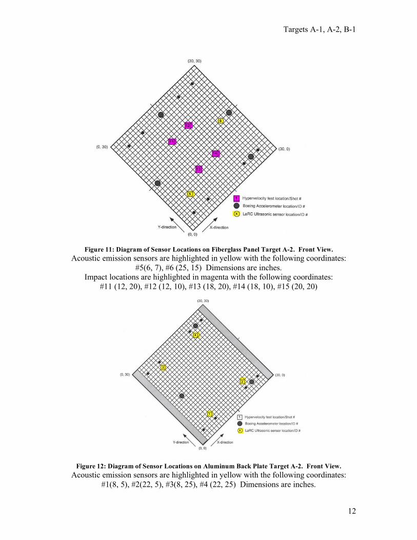
Figure 11: Diagram of Sensor Locations on Fiberglass Panel Target A-2. Front View.
Acoustic emission sensors are highlighted in yellow with the following coordinates:
#5(6, 7), #6 (25, 15) Dimensions are inches.
Impact locations are highlighted in magenta with the following coordinates:
#11 (12, 20), #12 (12, 10), #13 (18, 20), #14 (18, 10), #15 (20, 20)
Figure 12: Diagram of Sensor Locations on Aluminum Back Plate Target A-2. Front View.
Acoustic emission sensors are highlighted in yellow with the following coordinates:
#1(8, 5), #2(22, 5), #3(8, 25), #4 (22, 25) Dimensions are inches.

Targets A-1, A-2, B-1
13
On Target B-1, sensors 1-4 were coupled to the second fiberglass plate with Lord 202
acrylic adhesive. Sensors 5 and 6 were coupled to the first fiberglass plate and sensors 7
and 8 were coupled to the aluminum backplate. Diagrams of the sensor layout are shown
in Figure 13, Figure 14, and Figure 15.
Figure 13: Diagram of Sensor Locations on Fiberglass Plate 1 Target B-1. Front View.
Acoustic emission sensors are highlighted in yellow with the following coordinates:
#5(6, 7), #6 (25, 15) Dimensions are inches.
Impact locations are highlighted in magenta with the following coordinates:
#7 (12, 20), #8 (12, 10), #9 (18, 20), #10 (18, 10),
Figure 14: Diagram of Sensor Locations on Fiberglass Plate 2 Target B-1. Front View.
Acoustic emission sensors are highlighted in yellow with the following coordinates:
#1 (8, 5), #2 (22, 5), #3 (8, 25), #4 (25, 15) Dimensions are inches.

Targets A-1, A-2, B-1
14
Figure 15: Diagram of Sensor Locations on Aluminum Back Plate Target B-1. Front View.
Acoustic emission sensors are highlighted in yellow with the following coordinates:
#7(6, 7), #8 (25, 15) Dimensions are inches.
The piezoelectric sensor converted the sound wave energy to an electrical voltage. The
energy computed from the voltage data collected by each sensor channel is referred to as
the wave signal energy. (A complete description of the type of sensor used and
calibration is given in the General Introduction to this report.)
The wave signal energy for each channel was analyzed and compared to the impact
energy. A full description of the wave recording instrumentation is given in the General
Introduction to this report. (Each individual sensor was connected to a separate
amplification and filtering channel and the voltage produced by the sensor recorded and
stored on a computer.)
The wave signal energy was computed by integrating the squared voltage with respect to
time and dividing this number by the impedance at the preamp input. The voltage versus
time values of the wave, which were displayed in the waveform window on the computer
screen for each channel, were corrected for any applied gain (or attenuation).
Attenuation was the norm because hypervelocity impact produced very energetic signals
that in most cases would have saturated the A/D converter on the recording card in the
computer had the amplitude not been reduced.
Targets A-1, A-2, B-1
15
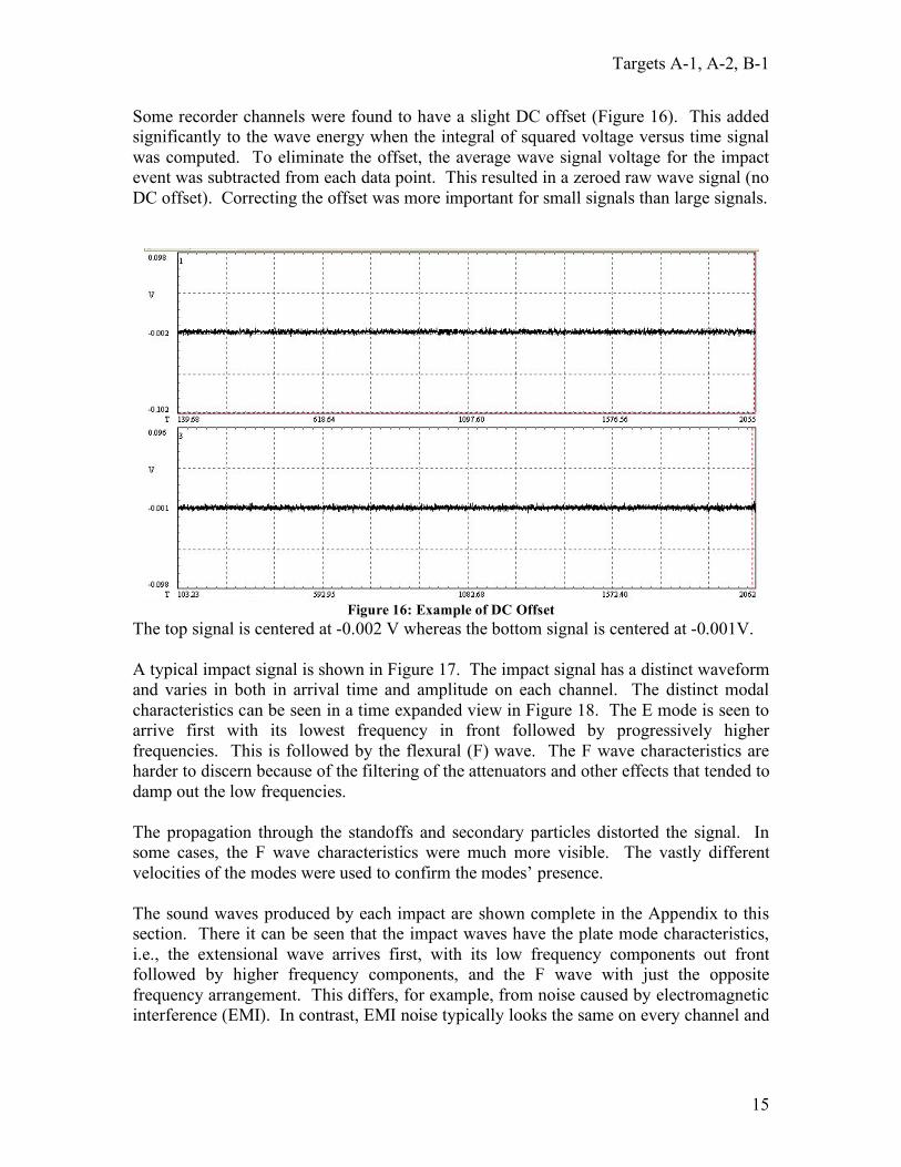
Some recorder channels were found to have a slight DC offset (Figure 16). This added
significantly to the wave energy when the integral of squared voltage versus time signal
was computed. To eliminate the offset, the average wave signal voltage for the impact
event was subtracted from each data point. This resulted in a zeroed raw wave signal (no
DC offset). Correcting the offset was more important for small signals than large signals.
Figure 16: Example of DC Offset
The top signal is centered at -0.002 V whereas the bottom signal is centered at -0.001V.
A typical impact signal is shown in Figure 17. The impact signal has a distinct waveform
and varies in both in arrival time and amplitude on each channel. The distinct modal
characteristics can be seen in a time expanded view in Figure 18. The E mode is seen to
arrive first with its lowest frequency in front followed by progressively higher
frequencies. This is followed by the flexural (F) wave. The F wave characteristics are
harder to discern because of the filtering of the attenuators and other effects that tended to
damp out the low frequencies.
The propagation through the standoffs and secondary particles distorted the signal. In
some cases, the F wave characteristics were much more visible. The vastly different
velocities of the modes were used to confirm the modes’ presence.
The sound waves produced by each impact are shown complete in the Appendix to this
section. There it can be seen that the impact waves have the plate mode characteristics,
i.e., the extensional wave arrives first, with its low frequency components out front
followed by higher frequency components, and the F wave with just the opposite
frequency arrangement. This differs, for example, from noise caused by electromagnetic
interference (EMI). In contrast, EMI noise typically looks the same on every channel and

Targets A-1, A-2, B-1
16
arrives simultaneously (Figure 19). EMI exhibits no plate wave propagation
characteristics.
Figure 17: A-2 Impact Signal for Shot #11
Figure 18: Detail of A-2 Impact Signal for Shot #11, Sensors 2 and 4

Targets A-1, A-2, B-1
17
2...G
EESW
raw=
Figure 19: A-2 Electromagnetic Interference for Shot #11
The MAE software computed the raw wave signal energy in Joules uncorrected for any
analog gain or attenuation that may have been applied to the signal path. In order to
compare the wave energies from shot to shot, the raw wave signal energy is converted by
applying Equation 1 where Eraw is the energy computed using the recorded wave (with
DC offset eliminated) and G is the system gain.
Equation 1
The gain G is computed by converting the logarithmic gain, M, in decibels with
Equation 2 or 3.
M dB = 20 Log10 (G) Equation 2
2010
M
G = Equation 3
The gains, raw wave signals, and wave energies for each shot are listed in the data tables
in the Appendix to this section.
High velocity impact produced signals on the order of a few volts directly out of the
transducer. These were much larger signals than typically found in most acoustic
emission measurements of, say, crack growth in metals. For most shots, attenuators were

Targets A-1, A-2, B-1
18
placed in the signal lines between the sensors and the digital recorders. Greater
attenuation was applied for the higher energy shots which made the raw energy appear to
be much less. The energy was restored to its full value by compensating in the analysis
for the greater attenuation, Equation 3 above.
Results
The most important quantities used in the analysis of the wave signals were the wave
signal energy and projectile kinetic energy for each shot. These are given in Table 1
along with the test number and impactor diameter. Wave signal energy is the sum of the
energy, in Joules, detected by all of the sensors. Kinetic energy is calculated based on the
velocity and mass of projectile (density of aluminum = 2700 kg/m3) according to the
usual formula K.E. = mv2/2. As will be seen, the kinetic energy correlated fairly well
with the damage. Normal KE is just the kinetic energy associated with the projectile
velocity component normal to the target surface at the point of impact.
Test Imp Dia
Kinetic Energy W.S.E.
No. mm J nJ
A1-1 1.0 31.83 3.836E+01
A1-2 1.4 87.59 1.262E+03
A1-3 1.6 128.81 1.915E-01
A1-4
A1-5 5.6 5841.76 9.453E+03
A1-6 6.0 7101.57 6.447E+03
B1-7 1.6 134.67 3.168E+05
B1-8 2.0 257.65 2.276E+03
B1-9 5.6 6013.32 2.904E+04
B1-10 6.0 7164.18 3.723E+04
A2-11 1.0 31.92 2.096E+02
A2-12 1.4 85.00 1.032E+03
A2-13 1.6 129.58 3.345E+03
A2-14 2.0 257.65 4.958E+03
A2-15 0.4 2.01 2.548E+00
Table 1: Kinetic Energy and Wave Signal Energy for Fiberglass Panel Target A-1, B-1, and A-2.
No data was available for shot #4.
The damage for each shot is given in Table 2. The crater volume damage is the product
of the recorded length, width, and depth measurements on the front side of the panel for
each impact. Damage area is the product of recorded length and width measurements on
the front side of the panel. Examples of impact damage are Figure 20, Figure 21, and
Figure 22.
Kinetic Energy
Crater Volume
Damage Area
Test No. J mm3 mm
2
A1-1 31.83 126.0 80.0
A1-2 87.59 225.0 229.5
A1-3 128.81 643.5 208.0
A1-4 1244.9* 513.0
A1-5 5841.76 2386.6* 513.0
A1-6 7101.57 4235.5* 89900.0
B1-7 134.67 180.0 289.0
B1-8 257.65 73.5 391.0
B1-9 6013.32 3016.4* 3350.0

Targets A-1, A-2, B-1
19
Table 2: Damage Results for Fiberglass Panel Targets A-1, B-1 and A-2.
* = Hole. No kinetic energy data was available for shot #4
Figure 20: A-1 Shot #5 Impact Damage
Figure 21: B-1 Shot #10 Impact Damage
Targets A-1, A-2, B-1
20
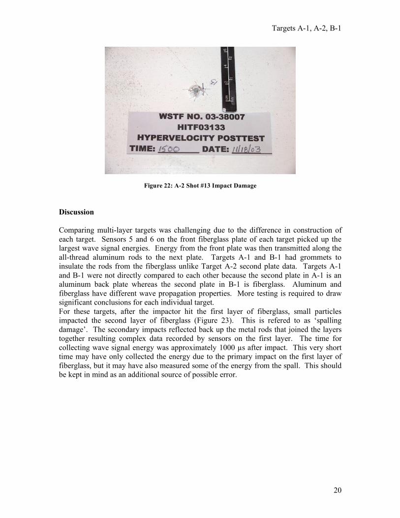
Figure 22: A-2 Shot #13 Impact Damage
Discussion
Comparing multi-layer targets was challenging due to the difference in construction of
each target. Sensors 5 and 6 on the front fiberglass plate of each target picked up the
largest wave signal energies. Energy from the front plate was then transmitted along the
all-thread aluminum rods to the next plate. Targets A-1 and B-1 had grommets to
insulate the rods from the fiberglass unlike Target A-2 second plate data. Targets A-1
and B-1 were not directly compared to each other because the second plate in A-1 is an
aluminum back plate whereas the second plate in B-1 is fiberglass. Aluminum and
fiberglass have different wave propagation properties. More testing is required to draw
significant conclusions for each individual target.
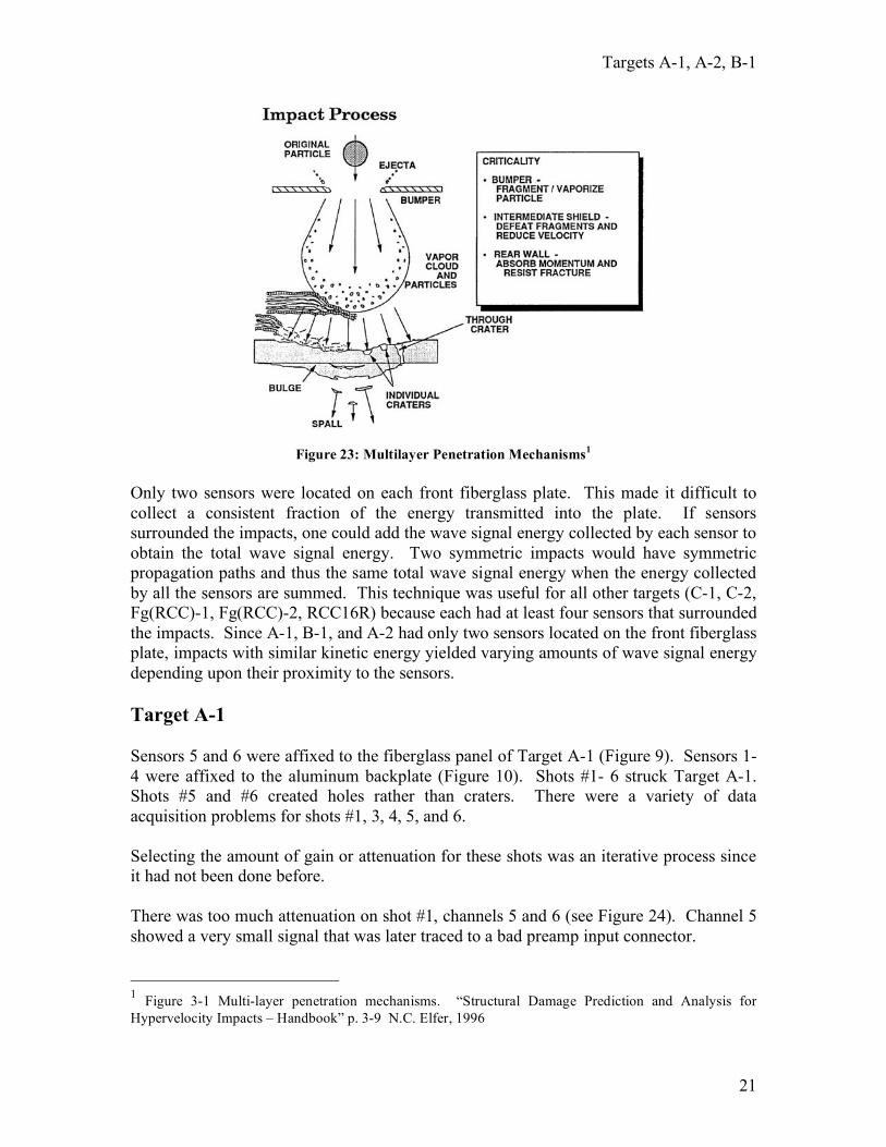
For these targets, after the impactor hit the first layer of fiberglass, small particles
impacted the second layer of fiberglass (Figure 23). This is refered to as ‘spalling
damage’. The secondary impacts reflected back up the metal rods that joined the layers
together resulting complex data recorded by sensors on the first layer. The time for
collecting wave signal energy was approximately 1000 !s after impact. This very short
time may have only collected the energy due to the primary impact on the first layer of
fiberglass, but it may have also measured some of the energy from the spall. This should
be kept in mind as an additional source of possible error.
Targets A-1, A-2, B-1
21
Figure 23: Multilayer Penetration Mechanisms1
Only two sensors were located on each front fiberglass plate. This made it difficult to
collect a consistent fraction of the energy transmitted into the plate. If sensors
surrounded the impacts, one could add the wave signal energy collected by each sensor to
obtain the total wave signal energy. Two symmetric impacts would have symmetric
propagation paths and thus the same total wave signal energy when the energy collected
by all the sensors are summed. This technique was useful for all other targets (C-1, C-2,
Fg(RCC)-1, Fg(RCC)-2, RCC16R) because each had at least four sensors that surrounded
the impacts. Since A-1, B-1, and A-2 had only two sensors located on the front fiberglass
plate, impacts with similar kinetic energy yielded varying amounts of wave signal energy
depending upon their proximity to the sensors.
Target A-1
Sensors 5 and 6 were affixed to the fiberglass panel of Target A-1 (Figure 9). Sensors 1-
4 were affixed to the aluminum backplate (Figure 10). Shots #1- 6 struck Target A-1.
Shots #5 and #6 created holes rather than craters. There were a variety of data
acquisition problems for shots #1, 3, 4, 5, and 6.
Selecting the amount of gain or attenuation for these shots was an iterative process since
it had not been done before.
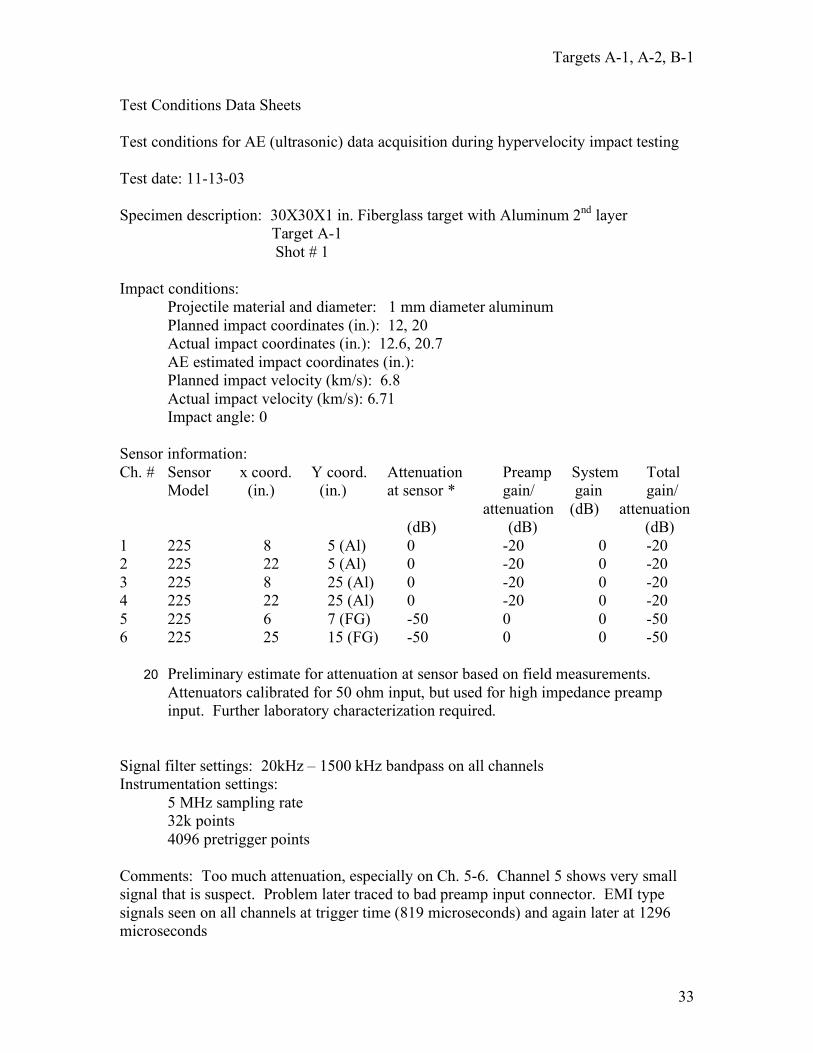
There was too much attenuation on shot #1, channels 5 and 6 (see Figure 24). Channel 5
showed a very small signal that was later traced to a bad preamp input connector.
1 Figure 3-1 Multi-layer penetration mechanisms. “Structural Damage Prediction and Analysis for
Hypervelocity Impacts – Handbook” p. 3-9 N.C. Elfer, 1996

Targets A-1, A-2, B-1
22
Figure 24: Impact Waveform for Shot #1. Notice the missing signal for sensor 5 in the bottom left
corner.
There was some saturation on sensor 2 for shot #3 and sensor 5 signals were not acquired
because of the bad preamp input connector.
No data was available for shot #4.
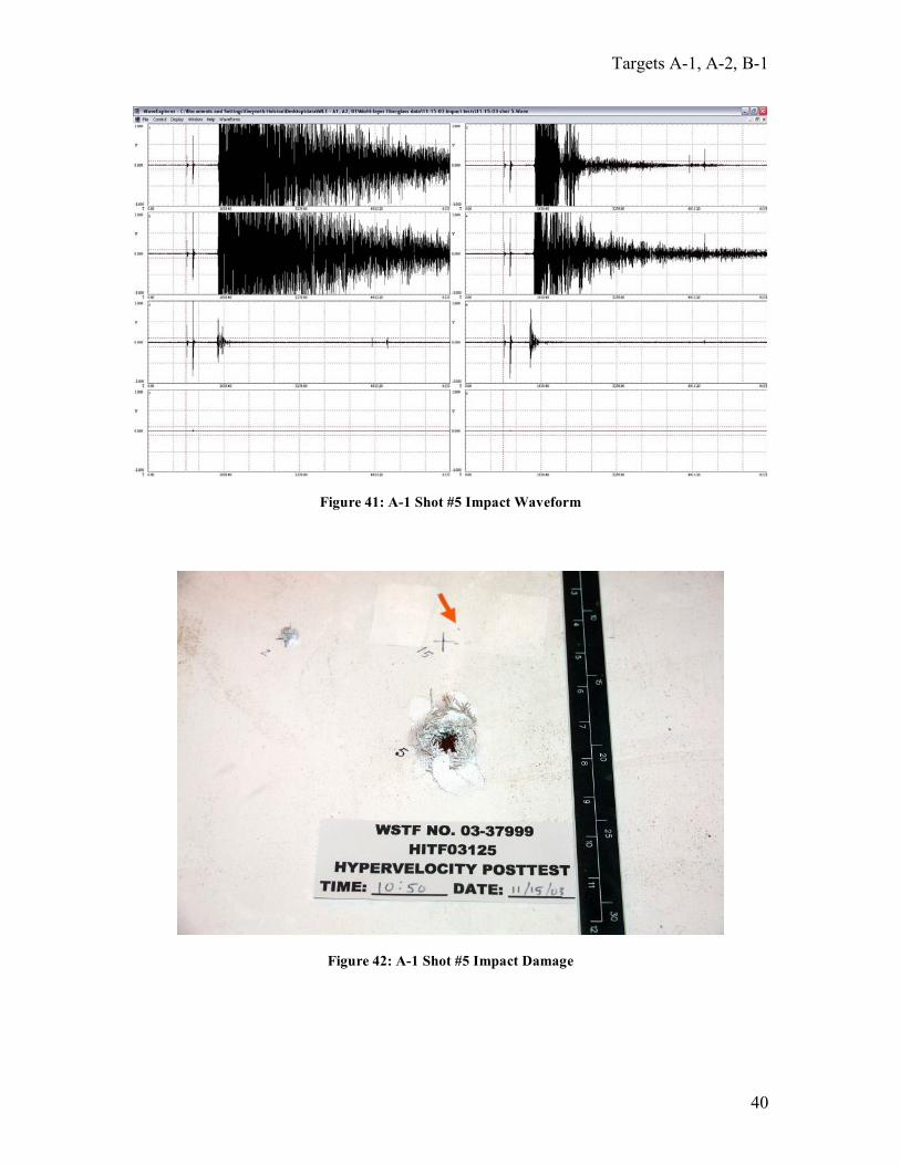
The gain was too high on channels 1-4 on shot #5 causing saturation (Figure 25). Large
EMI signals were observed on all channels at and just after trigger. Sensors 2 and 6 were
knocked off of the specimen and had to be rebonded before the next test.
Figure 25: Shot #5 Impact Waveform. Notice saturation on channels 1-4. Channels 2 and 6 have
shortened signals due to sensors being knocked off during impact.
On shot #6, sensor 1 was knocked off of the specimen during impact.
Good data was collected on Target A-1 fiberglass plate sensors 5 and 6 for shots #2, 5,
and 6. Predictably, the shots with high kinetic energies (shots #5 and 6) created holes and
also had high wave signal energies.

Targets A-1, A-2, B-1
23
Good data was collected on Target A-1 aluminum back plate sensors 1-4 only for shot #2.
Target A-2
Like A-1, sensors 5 and 6 were affixed to the fiberglass panel on Target A-2 (Figure 11).
Sensors 1-4 were affixed to the aluminum backplate (Figure 12). Shots #11- 15 struck
target A-2. Only shot #14 created a hole. There were data acquisition problems for shots
#11, 12, and 15.
Signals saturated on channels 1-3 for shot #11. Shots #12 and #15 suffered from the
aforementioned bad preamp input connector on sensor 5.
Acceptable data was collected on Target A-2 fiberglass plate sensors 5 and 6 for shots
#11, 13, and 14. The wave signal energy for these shots was plotted versus kinetic
energy in Figure 26. There was a trend of increasing wave signal energy with increasing
kinetic energy.
Multi-layer Fiberglass Kinetic Energy vs Wave Energy -
Face Plate Sensors
14
13
110
500
1000
1500
2000
2500
3000
3500
4000
4500
0 50 100 150 200 250 300
Kinetic Energy, Joules
Wa
ve
Sig
na
l E
ne
rgy
, n
J
Figure 26: Wave Signal Energy vs. Kinetic Energy on A-2 Fiberglass Plate (Sensors 5 and 6)
Good data was collected on Target A-2 aluminum back plate sensors 1-4 for shots #12-
15. The wave signal energy versus kinetic energy shows a linear trend in Figure 27.
Shot #14 created a hole and had a high wave signal energy.

Targets A-1, A-2, B-1
24
Aluminum Back Plate A1, A2
15
14
13
120
100
200
300
400
500
600
700
800
900
0 50 100 150 200 250 300
Kinetic Energy, Joules
Wa
ve
Sig
na
l E
ne
rgy
, n
J
Figure 27: Wave Signal Energy vs. Kinetic Energy for A-2 Aluminum Back Plate (Sensors 1-4)
The purpose of Targets A-1 and A-2 was to compare the effect that grommets had on
signals recorded by sensors on the aluminum back plate. Shots #12 (Target A-2) and #2
(Target A-1) had similar kinetic energies and similar wave signal energies on front panel
sensors 5 and 6. The difference in wave signal energies on the back plate due to the
existence of grommets was ~14 dB. This was confirmed by shots #13 and 3.
Target B-1
Sensors 5 and 6 were affixed to fiberglass plate 1 on Target B-1 (Figure 13). Sensors 1-4
were affixed to fiberglass panel 2 (Figure 14). Sensors 7 and 8 were affixed for the
aluminum back plate (Figure 15). Shots #7-10 struck target B-1. Shots #9 and 10 created
holes. There were data acquisition problems for shots #7, 9, and 10.
Signals were not acquired for shot #7 on channel 5 due to the aforementioned bad preamp
connector. The gain setting on channel 6 of shot #7 was questionable. Shots #3 and 7
had very similar kinetic energies and similar raw wave signals on sensors 6. The
calculated wave signal energy (Equation 1, p. 17 and Table 7, p. 64), however, was a
million times larger for shot #7 than shot #3 due to gain settings of -64 dB and -50 dB,
respectively. By comparing the raw signals (Figure 28), it was concluded that the gain
for shot #7 must be relatively close to the gain for shot #3, (-50 dB rather than the data
sheet value of -64 dB). If the gain on shot #7 were indeed -64 dB, its raw wave signal
(Figure 28) should have appeared at least four times larger than the signal for shot #3.

Targets A-1, A-2, B-1
25
Figure 28: Shot #3 Impact Waveform, Sensor 6 (left) and Shot #7 Impact Waveform, Sensor 6 (right)
Shot #9 was barely saturated on channel 4. There was too much attenuation on channels
7 and 8. Sensor 6 became disbonded as was evident in signal (Figure 29). Sensor 6 was
tested and replaced for the next shot.
Figure 29: Shot #9 Impact Waveform
Shot #10 was slightly saturated on channels 7 and 8 (Figure 30).

Targets A-1, A-2, B-1
26
Figure 30: Shot #10 Impact Waveform
Acceptable data was collected on Target B-1 fiberglass plate 1 sensors 5 and 6 for shots
#8 and 10. Shot #10 created a hole and had both a higher kinetic energy and wave signal
energy than shot #8.
Good data was collected on Target B-1 fiberglass plate 2 sensors 1-4 for shots #7, 8, and
10. All three shots were in keeping with the trend of increasing wave signal energy with
increasing kinetic energy.
Valid data was collected on Target B-1 aluminum back plate sensors 7 and 8 for shots #7
and 8. Consider the impact waveform for shot #7 (Figure 31). The wave signal first
arrived on sensors 5 and 6 since they were located on the first layer of fiberglass. It
arrived at sensor 5 slightly before sensor 6 because it impacted closer to sensor 5. These
channels clearly showed a large amplitude at initial impact that decreases with time. The
wave signal then proceeded to sensors 1-4 on the second layer of fiberglass. The wave
signal appears distorted because it had to travel through the all-thread rods from the first
fiberglass plate to the second. The wave reverberated inside the rods to create the types
of signals observed on sensors 1-4 and, finally, 7 and 8.

Targets A-1, A-2, B-1
27
Figure 31: Shot #7 Impact Waveform, Sensors 1-8
Location Analysis
Location of the source of a wave is part and parcel of the MAE technique just as it is in
SONAR methods. It contributes to understanding the type and magnitude of the source
and is a crucial step in tracking down and stopping leaks in manned spacecraft.
In these studies the location of the impact was known by visual observation. This
enabled a study of the accuracy of locating a source purely by analysis of the wave arrival
at different transducers. The source position was triangulated when the source to receiver
path was reasonably homogeneous. This was shown in detail for Target Fg(RCC)-1 and
the reader is referred to that Section of this Report.
The velocities of the direct arrivals were measured in advance. Pencil lead breaks were
done to create the modes. This is discussed under the section on Wave Propagation
below.
Wave Propagation
The wave signal energy collected by any given sensor is composed of direct energy and
reflected energy. After an impact occurs, a wave propagates radially outward from the
impact site. This direct wave is the first signal recorded by a sensor. When this wave
reaches the edges of the target, it is reflected back to the sensor. These reflected waves
are lower in amplitude than the direct waves and have later arrival times. In general,
reflected waves did not contribute not a significant fraction of the signal energy.

Targets A-1, A-2, B-1
28
The direct wave is composed of two types of waves: extensional and flexural.
Extensional waves have two displacements components with the larger displacements
perpendicular to the normal to the plate. A sensor on the surface detects the out-of-plane
component of the E wave. The largest displacement of the flexural wave motion is
perpendicular to the plane of the plate. This motion is caused by bending at the impact
location. The E and F modes have very distinct characteristics (see General Introduction)
that can be readily identified. For one thing, the front part of the E wave travels much
faster than any frequency component of the F wave.
Wave speed was determined by performing a lead break at one sensor and measuring the
time it takes for a direct wave to arrive at another sensor at a known distance away.
Except for the second fiberglass plate of B-1, there were only two sensors on each
fiberglass plate. This means that the wave speed could only be calculated in one
direction. Fortunately, the speeds of extensional and flexural waves were already
calculated for Targets C-1 and C-2. Extensional waves traveled 0.16 in/!s in the x-
direction, 0.16 in/!s in the y-direction and 0.14 in/!s in the diagonal. Flexural waves
traveled 0.06 in/!s in all directions.
In the fiberglass panel, fibers are aligned in the x and y directions (see Figure 9). In
addition to having slower speeds, waves that travel diagonally are attenuated more than
waves that travel along the fiber direction. This is generally known as material
anisotropy and is referred to here as diagonal attenuation. Compensation for this effect is
described in detail for Targets C-1 and C-2.
Conclusions
The results of the hypervelocity impact test on multi-layer Targets A-1, B-1, and A-2 are
as follows:
• Ultrasonic Sensors were successfully bonded to fiberglass Targets A-
1, B-1, and A-2 with a Lord 202 Acrylic Adhesive.
• Ultrasonic Sensors operated well in near-vacuum (6-8 Torr) inside the
vacuum chamber at Johnson Space Center’s White Sands Testing
Facility.2
• Impacts created detectable ultrasonic signals at high (>50 kHz)
frequencies which should be above flight noise.3
2 B1025 sensors also functioned well in deep vacuum of ESEM. Michael Horn, NASA LaRC, email 2005.

Targets A-1, A-2, B-1
29
• Ultrasonic signals were detected with small, lightweight sensors
capable of space flight.45
• Wave propagation characteristics of the cross-ply fiberglass target
were measured and used in the analysis of the wave signal energy.
• Wave signal energy correlated well with kinetic energy and impact
damage.
This test successfully demonstrated the ability for a wing leading edge
impact detection system (WLEIDS) to model the kinetic energy
response and material damage below, at and above complete
penetration of the projectile through the target.
Appendix
The appendices contain the information for each shot and the waveforms. For
completeness, and, for usefulness when judging the energy versus damage plots shown in
the discussion section above, tables are given at the end that summarize and group
together the data for the key test variables.
3 Based on measurement of noise spectra on F16 bulkhead at full throttle, there will not be significant noise
power above 50kHz. 4 Sensors passed 18,000 g shock test. Henry Whitesel, Naval Surface Warfare Center, verbal
communication 1998. 5 DWC sensors survived intense radiation environment. Dane Spearing, LANL, verbal communication
2003.

Targets A-1, A-2, B-1
30
Figure 32: Target A-1 Drawing

Targets A-1, A-2, B-1
31
Figure 33: Target B-1 Drawing

Targets A-1, A-2, B-1
32
Figure 34: Target A-2 Drawing
Targets A-1, A-2, B-1
33
Test Conditions Data Sheets
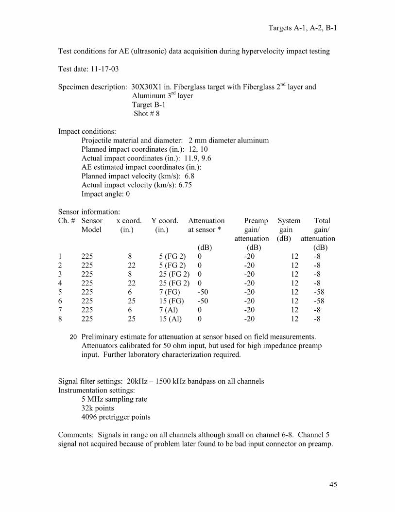
Test conditions for AE (ultrasonic) data acquisition during hypervelocity impact testing
Test date: 11-13-03
Specimen description: 30X30X1 in. Fiberglass target with Aluminum 2nd
layer
Target A-1
Shot # 1
Impact conditions:
Projectile material and diameter: 1 mm diameter aluminum
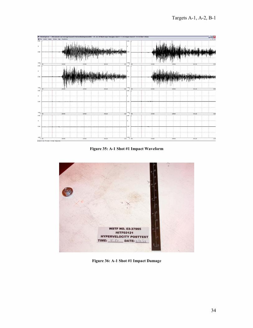
Planned impact coordinates (in.): 12, 20
Actual impact coordinates (in.): 12.6, 20.7
AE estimated impact coordinates (in.):
Planned impact velocity (km/s): 6.8
Actual impact velocity (km/s): 6.71
Impact angle: 0
Sensor information:
Ch. # Sensor x coord. Y coord. Attenuation Preamp System Total
Model (in.) (in.) at sensor * gain/ gain gain/
attenuation (dB) attenuation
(dB) (dB) (dB)
1 225 8 5 (Al) 0 -20 0 -20
2 225 22 5 (Al) 0 -20 0 -20
3 225 8 25 (Al) 0 -20 0 -20
4 225 22 25 (Al) 0 -20 0 -20
5 225 6 7 (FG) -50 0 0 -50
6 225 25 15 (FG) -50 0 0 -50
20 Preliminary estimate for attenuation at sensor based on field measurements.
Attenuators calibrated for 50 ohm input, but used for high impedance preamp
input. Further laboratory characterization required.
Signal filter settings: 20kHz – 1500 kHz bandpass on all channels
Instrumentation settings:
5 MHz sampling rate
32k points
4096 pretrigger points
Comments: Too much attenuation, especially on Ch. 5-6. Channel 5 shows very small
signal that is suspect. Problem later traced to bad preamp input connector. EMI type
signals seen on all channels at trigger time (819 microseconds) and again later at 1296
microseconds
Targets A-1, A-2, B-1
34
Figure 35: A-1 Shot #1 Impact Waveform
Figure 36: A-1 Shot #1 Impact Damage

Targets A-1, A-2, B-1
35
Test conditions for AE (ultrasonic) data acquisition during hypervelocity impact testing
Test date: 11-14-03
Specimen description: 30X30X1 in. Fiberglass target with Aluminum 2nd
layer
Target A-1
Shot # 2
Impact conditions:
Projectile material and diameter: 1.4 mm diameter aluminum
Planned impact coordinates (in.): 16, 20
Actual impact coordinates (in.): 16.1, 20.1
AE estimated impact coordinates (in.):
Planned impact velocity (km/s): 6.8
Actual impact velocity (km/s): 6.72
Impact angle: 0
Sensor information:
Ch. # Sensor x coord. Y coord. Attenuation Preamp System Total
Model (in.) (in.) at sensor * gain/ gain gain/
attenuation (dB) attenuation
(dB) (dB) (dB)
1 225 8 5 (Al) 0 0 6 6
2 225 22 5 (Al) 0 0 6 6
3 225 8 25 (Al) 0 0 6 6
4 225 22 25 (Al) 0 0 6 6
5 225 6 7 (FG) -50 0 9 -41
6 225 25 15 (FG) -50 0 9 -41
20 Preliminary estimate for attenuation at sensor based on field measurements.
Attenuators calibrated for 50 ohm input, but used for high impedance preamp
input. Further laboratory characterization required.
Signal filter settings: 20kHz – 1500 kHz bandpass on all channels
Instrumentation settings:
5 MHz sampling rate
32k points
4096 pretrigger points
Comments: All signals in range. Channel 5 acquired on this shot.

Targets A-1, A-2, B-1
36
Figure 37: A-1 Shot #2 Impact Waveform
Figure 38: A-1 Shot #2 Impact Damage

Targets A-1, A-2, B-1
37
Test conditions for AE (ultrasonic) data acquisition during hypervelocity impact testing
Test date: 11-14-03
Specimen description: 30X30X1 in. Fiberglass target with Aluminum 2nd
layer
Target A-1
Shot # 3
Impact conditions:
Projectile material and diameter: 1.6 mm diameter aluminum
Planned impact coordinates (in.): 20, 10
Actual impact coordinates (in.): 20.2, 9.75
AE estimated impact coordinates (in.):
Planned impact velocity (km/s): 6.8
Actual impact velocity (km/s): 6.67
Impact angle: 0
Sensor information:
Ch. # Sensor x coord. Y coord. Attenuation Preamp System Total
Model (in.) (in.) at sensor * gain/ gain gain/
attenuation (dB) attenuation
(dB) (dB) (dB)
1 225 8 5 (Al) 0 0 0 0
2 225 22 5 (Al) 0 0 0 0
3 225 8 25 (Al) 0 0 0 0
4 225 22 25 (Al) 0 0 0 0
5 225 6 7 (FG) -50 0 0 -50
6 225 25 15 (FG) -50 0 0 -50
20 Preliminary estimate for attenuation at sensor based on field measurements.
Attenuators calibrated for 50 ohm input, but used for high impedance preamp
input. Further laboratory characterization required.
Signal filter settings: 20kHz – 1500 kHz bandpass on all channels
Instrumentation settings:
5 MHz sampling rate
32k points
4096 pretrigger points
Comments: All signals in range except some saturation on channel 2. Channel 5 data not
acquired because of problem later found to be bad input connector on preamp.

Targets A-1, A-2, B-1
38
Figure 39: A-1 Shot #3 Impact Waveform
Figure 40: A-1 Shot #3 Impact Damage

Targets A-1, A-2, B-1
39
Test conditions for AE (ultrasonic) data acquisition during hypervelocity impact testing
Test date: 11-15-03
Specimen description: 30X30X1 in. Fiberglass target with Aluminum 2nd
layer
Target A-1
Shot # 5
Impact conditions:
Projectile material and diameter: 5.6 mm diameter aluminum
Planned impact coordinates (in.): 20, 17
Actual impact coordinates (in.): 20.2, 17.1
AE estimated impact coordinates (in.):
Planned impact velocity (km/s): 6.8
Actual impact velocity (km/s): 6.86
Impact angle: 0
Sensor information:
Ch. # Sensor x coord. Y coord. Attenuation Preamp System Total
Model (in.) (in.) at sensor * gain/ gain gain/
attenuation (dB) attenuation
(dB) (dB) (dB)
1 225 8 5 (Al) 0 0 36 36
2 225 22 5 (Al) 0 0 36 36
3 225 8 25 (Al) 0 0 36 36
4 225 22 25 (Al) 0 0 36 36
5 225 6 7 (FG) -50 -20 33 -37
6 225 25 15 (FG) -50 -20 33 -37
20 Preliminary estimate for attenuation at sensor based on field measurements.
Attenuators calibrated for 50 ohm input, but used for high impedance preamp
input. Further laboratory characterization required.
Signal filter settings: 20kHz – 1500 kHz bandpass on all channels
Instrumentation settings:
5 MHz sampling rate
32k points
4096 pretrigger points
Comments: Gain improperly set much too high on Channels 1-4 causing much
saturation. Signals obtained and in range on Ch. 5-6. Large EMI signals observed on all
channels at and just after trigger. Sensors 2 and 6 were knocked off of the specimen and
had to be � ebounded before the next test.
Targets A-1, A-2, B-1
40
Figure 41: A-1 Shot #5 Impact Waveform
Figure 42: A-1 Shot #5 Impact Damage

Targets A-1, A-2, B-1
41
Test conditions for AE (ultrasonic) data acquisition during hypervelocity impact testing
Test date: 11-15-03
Specimen description: 30X30X1 in. Fiberglass target with Aluminum 2nd
layer
Target A-1
Shot # 6
Impact conditions:
Projectile material and diameter: 6.0 mm diameter aluminum
Planned impact coordinates (in.): 12, 10
Actual impact coordinates (in.): 11.9, 9.75
AE estimated impact coordinates (in.):
Planned impact velocity (km/s): 6.8
Actual impact velocity (km/s): 6.82
Impact angle: 0
Sensor information:
Ch. # Sensor x coord. Y coord. Attenuation Preamp System Total
Model (in.) (in.) at sensor * gain/ gain gain/
attenuation (dB) attenuation
(dB) (dB) (dB)
1 225 8 5 (Al) 0 0 12 12
2 225 22 5 (Al) 0 0 12 12
3 225 8 25 (Al) 0 0 12 12
4 225 22 25 (Al) 0 0 12 12
5 225 6 7 (FG) -50 -20 12 -58
6 225 25 15 (FG) -50 -20 12 -58
20 Preliminary estimate for attenuation at sensor based on field measurements.
Attenuators calibrated for 50 ohm input, but used for high impedance preamp
input. Further laboratory characterization required.
Signal filter settings: 20kHz – 1500 kHz bandpass on all channels
Instrumentation settings:
5 MHz sampling rate
32k points
4096 pretrigger points
Comments: Signals in range although very small on Ch. 5-6. Sensor 1 was knocked off
specimen during impact. A much shortened time signal is usually observed when the
sensor comes off the target.

Targets A-1, A-2, B-1
42
Figure 43: A-1 Shot #6 Impact Waveform
Figure 44: A-1 Shot #6 Impact Damage

Targets A-1, A-2, B-1
43
Test conditions for AE (ultrasonic) data acquisition during hypervelocity impact testing
Test date: 11-17-03
Specimen description: 30X30X1 in. Fiberglass target with Fiberglass 2nd
layer and
Aluminum 3rd
layer
Target B-1
Shot # 7
Impact conditions:
Projectile material and diameter: 1.6 mm diameter aluminum
Planned impact coordinates (in.): 12, 20
Actual impact coordinates (in.): 11.8, 19.6
AE estimated impact coordinates (in.):
Planned impact velocity (km/s): 6.8
Actual impact velocity (km/s): 6.82
Impact angle: 0
Sensor information:
Ch. # Sensor x coord. Y coord. Attenuation Preamp System Total
Model (in.) (in.) at sensor * gain/ gain gain/
attenuation (dB) attenuation
(dB) (dB) (dB)
1 225 8 5 (FG 2) 0 0 6 6
2 225 22 5 (FG 2) 0 0 6 6
3 225 8 25 (FG 2) 0 0 6 6
4 225 22 25 (FG 2) 0 0 6 6
5 225 6 7 (FG) -50 -20 6 -64
6 225 25 15 (FG) -50 -20 6 -64
7 225 6 7 (Al) 0 0 3 3
8 225 25 15 (Al) 0 0 3 3
20 Preliminary estimate for attenuation at sensor based on field measurements.
Attenuators calibrated for 50 ohm input, but used for high impedance preamp
input. Further laboratory characterization required.
Signal filter settings: 20kHz – 1500 kHz bandpass on all channels
Instrumentation settings:
5 MHz sampling rate
32k points
4096 pretrigger points
Comments: Signals in range on all channels and channel 5 signal acquired. EMI near
trigger much smaller.

Targets A-1, A-2, B-1
44
Figure 45: B-1 Shot #7 Impact Waveform
Figure 46: B-1 Shot #7 Impact Waveform
Targets A-1, A-2, B-1
45
Test conditions for AE (ultrasonic) data acquisition during hypervelocity impact testing
Test date: 11-17-03
Specimen description: 30X30X1 in. Fiberglass target with Fiberglass 2nd
layer and
Aluminum 3rd
layer
Target B-1
Shot # 8
Impact conditions:
Projectile material and diameter: 2 mm diameter aluminum
Planned impact coordinates (in.): 12, 10
Actual impact coordinates (in.): 11.9, 9.6
AE estimated impact coordinates (in.):
Planned impact velocity (km/s): 6.8
Actual impact velocity (km/s): 6.75
Impact angle: 0
Sensor information:
Ch. # Sensor x coord. Y coord. Attenuation Preamp System Total
Model (in.) (in.) at sensor * gain/ gain gain/
attenuation (dB) attenuation
(dB) (dB) (dB)
1 225 8 5 (FG 2) 0 -20 12 -8
2 225 22 5 (FG 2) 0 -20 12 -8
3 225 8 25 (FG 2) 0 -20 12 -8
4 225 22 25 (FG 2) 0 -20 12 -8
5 225 6 7 (FG) -50 -20 12 -58
6 225 25 15 (FG) -50 -20 12 -58
7 225 6 7 (Al) 0 -20 12 -8
8 225 25 15 (Al) 0 -20 12 -8
20 Preliminary estimate for attenuation at sensor based on field measurements.
Attenuators calibrated for 50 ohm input, but used for high impedance preamp
input. Further laboratory characterization required.
Signal filter settings: 20kHz – 1500 kHz bandpass on all channels
Instrumentation settings:
5 MHz sampling rate
32k points
4096 pretrigger points
Comments: Signals in range on all channels although small on channel 6-8. Channel 5
signal not acquired because of problem later found to be bad input connector on preamp.

Targets A-1, A-2, B-1
46
Figure 47: B-1 Shot #8 Impact Waveform
Figure 48: B-1 Shot #8 Impact Damage

Targets A-1, A-2, B-1
47
Test conditions for AE (ultrasonic) data acquisition during hypervelocity impact testing
Test date: 11-19-03
Specimen description: 30X30X1 in. Fiberglass target with Fiberglass 2nd
layer and
Aluminum 3rd
layer
Target B-1
Shot # 9
Impact conditions:
Projectile material and diameter: 5.6 mm diameter aluminum
Planned impact coordinates (in.): 18, 20
Actual impact coordinates (in.): 18, 19.2
AE estimated impact coordinates (in.):
Planned impact velocity (km/s): 6.8
Actual impact velocity (km/s): 6.96
Impact angle: 0
Sensor information:
Ch. # Sensor x coord. Y coord. Attenuation Preamp System Total
Model (in.) (in.) at sensor * gain/ gain gain/
attenuation (dB) attenuation
(dB) (dB) (dB)
1 225 8 5 (FG 2) -50 0 12 -38
2 225 22 5 (FG 2) -50 0 12 -38
3 225 8 25 (FG 2) -50 0 12 -38
4 225 22 25 (FG 2) -50 0 12 -38
5 225 6 7 (FG) -50 -20 18 -52
6 225 25 15 (FG) -50 -20 18 -52
7 225 6 7 (Al) -50 20 12 -18
8 225 25 15 (Al) -50 20 12 -18
20 Preliminary estimate for attenuation at sensor based on field measurements.
Attenuators calibrated for 50 ohm input, but used for high impedance preamp
input. Further laboratory characterization required.
Signal filter settings: 20kHz – 1500 kHz bandpass on all channels
Instrumentation settings:
5 MHz sampling rate
32k points
4096 pretrigger points
Comments: Saturation on Channel 4 only. Too much attenuation on channels 7-8. EMI
signals observed at trigger time. Sensor 6 became disbanded as was evident in signal.
Another EMI signal generated when sensor 6 stops functioning. Sensor 6 was tested and
replace for next shot.

Targets A-1, A-2, B-1
48
Figure 49: B-1 Shot # 9 Impact Waveform
Figure 50: B-1 Shot # 9 Impact Damage

Targets A-1, A-2, B-1
49
Test conditions for AE (ultrasonic) data acquisition during hypervelocity impact testing
Test date: 11-19-03
Specimen description: 30X30X1 in. Fiberglass target with Fiberglass 2nd
layer and
Aluminum 3rd
layer
Target B-1
Shot # 10
Impact conditions:
Projectile material and diameter: 6 mm diameter aluminum
Planned impact coordinates (in.): 18, 10
Actual impact coordinates (in.): 17.8, 10.1
AE estimated impact coordinates (in.):
Planned impact velocity (km/s): 6.8
Actual impact velocity (km/s): 6.85
Impact angle: 0
Sensor information:
Ch. # Sensor x coord. Y coord. Attenuation Preamp System Total
Model (in.) (in.) at sensor * gain/ gain gain/
attenuation (dB) attenuation
(dB) (dB) (dB)
1 225 8 5 (FG 2) -50 -20 18 -52
2 225 22 5 (FG 2) -50 -20 18 -52
3 225 8 25 (FG 2) -50 -20 18 -52
4 225 22 25 (FG 2) -50 -20 18 -52
5 225 6 7 (FG) -50 -20 12 -58
6 225 25 15 (FG) -50 -20 12 -58
7 225 6 7 (Al) 0 0 3 3
8 225 25 15 (Al) 0 0 3 3
20 Preliminary estimate for attenuation at sensor based on field measurements.
Attenuators calibrated for 50 ohm input, but used for high impedance preamp
input. Further laboratory characterization required.
Signal filter settings: 20kHz – 1500 kHz bandpass on all channels
Instrumentation settings:
5 MHz sampling rate
32k points
4096 pretrigger points
Comments: Saturation on Channel 7-8. EMI pulses seen at trigger time and alos later in
signals. No sensors debonded during test.

Targets A-1, A-2, B-1
50
Figure 51: B-1 Shot #10 Impact Waveform
Figure 52: B-1 Shot #10 Impact Damage

Targets A-1, A-2, B-1
51
Test conditions for AE (ultrasonic) data acquisition during hypervelocity impact testing
Test date: 11-18-03
Specimen description: 30X30X1 in. Fiberglass target with Aluminum 2nd
layer
No grommets around standoff rods
Target A-2
Shot # 11
Impact conditions:
Projectile material and diameter: 1 mm diameter aluminum
Planned impact coordinates (in.): 12, 20
Actual impact coordinates (in.): 11.8, 19.7
AE estimated impact coordinates (in.):
Planned impact velocity (km/s): 6.8
Actual impact velocity (km/s): 6.72
Impact angle: 0
Sensor information:
Ch. # Sensor x coord. Y coord. Attenuation Preamp System Total
Model (in.) (in.) at sensor * gain/ gain gain/
attenuation (dB) attenuation
(dB) (dB) (dB)
1 225 8 5 (Al) 0 0 12 12
2 225 22 5 (Al) 0 0 12 12
3 225 8 25 (AL) 0 0 12 12
4 225 22 25 (AL) 0 0 12 12
5 225 6 7 (FG) -50 0 12 -38
6 225 25 15 (FG) -50 0 12 -38
20 Preliminary estimate for attenuation at sensor based on field measurements.
Attenuators calibrated for 50 ohm input, but used for high impedance preamp
input. Further laboratory characterization required.
Signal filter settings: 20kHz – 1500 kHz bandpass on all channels
Instrumentation settings:
5 MHz sampling rate
32k points
4096 pretrigger points
Comments: Signals saturated on channels 1-3 later in signal, not in direct arrivals.
Signal acquired for this impact on channel 5. Channels 1-4 compared to Shot 1 on panel
A-1 (with grommets) and showed ~14 dB higher amplitude without grommets. Channel
6 was similar in amplitude to the Shot 1 Channel 6.

Targets A-1, A-2, B-1
52
Figure 53: A-2 Shot #11 Impact Waveform
Figure 54: A-2 Shot #11 Impact Damage

Targets A-1, A-2, B-1
53
Test conditions for AE (ultrasonic) data acquisition during hypervelocity impact testing
Test date: 11-18-03
Specimen description: 30X30X1 in. Fiberglass target with Aluminum 2nd
layer
No grommets around standoff rods
Target A-2
Shot # 12
Impact conditions:
Projectile material and diameter: 1.4 mm diameter aluminum
Planned impact coordinates (in.): 18, 20
Actual impact coordinates (in.): 17.5, 19.9
AE estimated impact coordinates (in.):
Planned impact velocity (km/s): 6.8
Actual impact velocity (km/s): 6.62
Impact angle: 0
Sensor information:
Ch. # Sensor x coord. Y coord. Attenuation Preamp System Total
Model (in.) (in.) at sensor * gain/ gain gain/
attenuation (dB) attenuation
(dB) (dB) (dB)
1 225 8 5 (Al) 0 -20 9 9
2 225 22 5 (Al) 0 -20 9 9
3 225 8 25 (AL) 0 -20 9 9
4 225 22 25 (AL) 0 -20 9 9
5 225 6 7 (FG) -50 0 9 -41
6 225 25 15 (FG) -50 0 9 -41
20 Preliminary estimate for attenuation at sensor based on field measurements.
Attenuators calibrated for 50 ohm input, but used for high impedance preamp
input. Further laboratory characterization required.
Signal filter settings: 20kHz – 1500 kHz bandpass on all channels
Instrumentation settings:
5 MHz sampling rate
32k points
4096 pretrigger points
Comments: All signals in range. Channel 5 not recorded because of problem later
identified as bad input connector on preamp. Channels 1-4 compared to Shot 2 on panel
A-1 (with grommets) and showed ~14 dB higher amplitude without grommets. Channel
6 was similar in amplitude to the Shot 1 Channel 6.

Targets A-1, A-2, B-1
54
Figure 55: A-2 Shot #12 Impact Waveform
Figure 56: A-2 Shot #12 Impact Damage

Targets A-1, A-2, B-1
55
Test conditions for AE (ultrasonic) data acquisition during hypervelocity impact testing
Test date: 11-18-03
Specimen description: 30X30X1 in. Fiberglass target with Aluminum 2nd
layer
No grommets around standoff rods
Target A-2
Shot # 13
Impact conditions:
Projectile material and diameter: 1.6 mm diameter aluminum
Planned impact coordinates (in.): 12, 10
Actual impact coordinates (in.): 12.3, 10.1
AE estimated impact coordinates (in.):
Planned impact velocity (km/s): 6.8
Actual impact velocity (km/s): 6.69
Impact angle: 0
Sensor information:
Ch. # Sensor x coord. Y coord. Attenuation Preamp System Total
Model (in.) (in.) at sensor * gain/ gain gain/
attenuation (dB) attenuation
(dB) (dB) (dB)
1 225 8 5 (Al) 0 -20 3 -17
2 225 22 5 (Al) 0 -20 3 -17
3 225 8 25 (AL) 0 -20 3 -17
4 225 22 25 (AL) 0 -20 3 -17
5 225 6 7 (FG) -50 0 3 -47
6 225 25 15 (FG) -50 0 3 -47
20 Preliminary estimate for attenuation at sensor based on field measurements.
Attenuators calibrated for 50 ohm input, but used for high impedance preamp
input. Further laboratory characterization required.
Signal filter settings: 20kHz – 1500 kHz bandpass on all channels
Instrumentation settings:
5 MHz sampling rate
32k points
4096 pretrigger points
Comments: All signals in range. Preamp was replace on ch. 5 eliminating problem that
caused previous loss of data on this channel. Again, signals on ch 1-4 compared to shot 3
on panel A-1 (w/grommets) and similar ~14 dB signal change observed.
Test conditions for AE (ultrasonic) data acquisition during hypervelocity impact testing

Targets A-1, A-2, B-1
56
Figure 57: A-2 Shot #13 Impact Waveform
Figure 58: A-2 Shot #13 Impact Damage

Targets A-1, A-2, B-1
57
Test date: 11-18-03
Specimen description: 30X30X1 in. Fiberglass target with Aluminum 2nd
layer
No grommets around standoff rods
Target A-2
Shot # 14
Impact conditions:
Projectile material and diameter: 2 mm diameter aluminum
Planned impact coordinates (in.): 18, 10
Actual impact coordinates (in.): 18.6, 10.1
AE estimated impact coordinates (in.):
Planned impact velocity (km/s): 6.8
Actual impact velocity (km/s): 6.75
Impact angle: 0
Sensor information:
Ch. # Sensor x coord. Y coord. Attenuation Preamp System Total
Model (in.) (in.) at sensor * gain/ gain gain/
attenuation (dB) attenuation
(dB) (dB) (dB)
1 225 8 5 (Al) 0 -20 3 -17
2 225 22 5 (Al) 0 -20 3 -17
3 225 8 25 (AL) 0 -20 3 -17
4 225 22 25 (AL) 0 -20 3 -17
5 225 6 7 (FG) -50 0 3 -47
6 225 25 15 (FG) -50 0 3 -47
20 Preliminary estimate for attenuation at sensor based on field measurements.
Attenuators calibrated for 50 ohm input, but used for high impedance preamp
input. Further laboratory characterization required.
Signal filter settings: 20kHz – 1500 kHz bandpass on all channels
Instrumentation settings:
5 MHz sampling rate
32k points
4096 pretrigger points
Comments: Again all signals in range. No comparison with signal from shot 4 possible
as shot 4 data was lost because of a computer error.

Targets A-1, A-2, B-1
58
Figure 59: A-2 Shot #14 Impact Waveform
Figure 60: A-2 Shot #14 Impact Damage

Targets A-1, A-2, B-1
59
Test conditions for AE (ultrasonic) data acquisition during hypervelocity impact testing
Test date: 11-14-03
Specimen description: 30X30X1 in. Fiberglass target with Aluminum 2nd
layer
Target A-1
Shot # 15
Impact conditions:
Projectile material and diameter: 0.4 mm diameter aluminum
Planned impact coordinates (in.): 20, 20
Actual impact coordinates (in.): 20.4, 20.4
AE estimated impact coordinates (in.):
Planned impact velocity (km/s): 6.8
Actual impact velocity (km/s): 6.67
Impact angle: 0
Sensor information:
Ch. # Sensor x coord. Y coord. Attenuation Preamp System Total
Model (in.) (in.) at sensor * gain/ gain gain/
attenuation (dB) attenuation
(dB) (dB) (dB)
1 225 8 5 (Al) 0 0 30 30
2 225 22 5 (Al) 0 0 30 30
3 225 8 25 (Al) 0 0 30 30
4 225 22 25 (Al) 0 0 30 30
5 225 6 7 (FG) -50 0 33 -17
6 225 25 15 (FG) -50 0 33 -17
20 Preliminary estimate for attenuation at sensor based on field measurements.
Attenuators calibrated for 50 ohm input, but used for high impedance preamp
input. Further laboratory characterization required.
Signal filter settings: 20kHz – 1500 kHz bandpass on all channels
Instrumentation settings:
5 MHz sampling rate
32k points
4096 pretrigger points
Comments: All signals in range except. Very small signal on Channel 5 that is suspect
because of problem later found to be bad input connector on preamp.

Targets A-1, A-2, B-1
60
Figure 61: A-2 Shot #15 Impact Waveform
Figure 62: A-2 Shot #15 Impact Damage

Targets A-1, A-2, B-1
61
Test conditions for AE (ultrasonic) data acquisition during hypervelocity impact testing
Test date: 11-18-03
Specimen description: 30X30X1 in. Fiberglass target with Aluminum 2nd
layer
No grommets around standoff rods
Target A-2
Shot # 16
Impact conditions:
Projectile material and diameter: 0.4 mm diameter aluminum
Planned impact coordinates (in.): 12, 15
Actual impact coordinates (in.): missed target
AE estimated impact coordinates (in.):
Planned impact velocity (km/s): 6.8
Actual impact velocity (km/s): missed target
Impact angle: 0
Sensor information:
Ch. # Sensor x coord. Y coord. Attenuation Preamp System Total
Model (in.) (in.) at sensor * gain/ gain gain/
attenuation (dB) attenuation
(dB) (dB) (dB)
1 225 8 5 (Al) 0 0 15 15
2 225 22 5 (Al) 0 0 15 15
3 225 8 25 (AL) 0 0 15 15
4 225 22 25 (AL) 0 0 15 15
5 225 6 7 (FG) -50 0 27 -23
6 225 25 15 (FG) -50 0 27 -23
20 Preliminary estimate for attenuation at sensor based on field measurements.
Attenuators calibrated for 50 ohm input, but used for high impedance preamp
input. Further laboratory characterization required.
Signal filter settings: 20kHz – 1500 kHz bandpass on all channels
Instrumentation settings:
5 MHz sampling rate
32k points
4096 pretrigger points
Comments: System triggered, but no signals detected. Projectile missed target.

Targets A-1, A-2, B-1
62
Data Tables
Test Imp Dia
Imp Vel
Imp Ang K.E. Location
No. mm km/s deg J x y
A1-1 1.0 6.71 90 31.83 12.6 20.7
A1-2 1.4 6.72 90 87.59 16.1 20.1
A1-3 1.6 6.67 90 128.81 20.2 9.75
A1-5 5.6 6.86 90 5841.76 20.2 17.1
A1-6 6.0 6.82 90 7101.57 11.9 9.75
B1-7 1.6 6.82 90 134.67 11.8 19.6
B1-8 2.0 6.75 90 257.65 11.9 9.6
B1-9 5.6 6.96 90 6013.32 18 19.2
B1-10 6.0 6.85 90 7164.18 17.8 10.1
A2-11 1.0 6.72 90 31.92 11.8 19.7
A2-12 1.4 6.62 90 85.00 17.5 19.9
A2-13 1.6 6.69 90 129.58 12.3 10.1
A2-14 2.0 6.75 90 257.65 18.6 10.1
A2-15 0.4 6.67 90 2.01 20.4 20.4
Table 3: A-1, B-1, and A-2 Impactor Diameter, Impactor Velocity, Impactor Angle, Kinetic Energy,
and Location
Shot #4 had no recorded kinetic energy.
Kinetic Crater Dims Crater Damage Dims Damage
Test Energy x y z Vol x y Area
No. J mm mm mm mm3 mm mm mm
2
A1-1 31.83 7.0 9.0 2.0 126.0 8.0 10.0 80.0
A1-2 87.59 9.0 10.0 2.5 225.0 13.5 17.0 229.5
A1-3 128.81 11.0 13.0 4.5 643.5 13.0 16.0 208.0
A1-4 13.0 13.0 7.4 1244.9 19.0 27.0 513.0
A1-5 5841.76 18.0 18.0 7.4 2386.6 19.0 27.0 513.0
A1-6 7101.57 23.0 25.0 7.4 4235.5 290.0 310.0 89900.0
B1-7 134.67 6.0 6.0 5.0 180.0 17.0 17.0 289.0
B1-8 257.65 7.0 7.0 1.5 73.5 23.0 17.0 391.0
B1-9 6013.32 21.0 19.5 7.4 3016.4 67.0 50.0 3350.0
B1-10 7164.18 25.5 24.0 7.4 4508.0 57.0 34.0 1938.0
A2-11 31.92 3.5 3.0 2.0 21.0 9.0 7.0 63.0
A2-12 85.00 5.0 6.0 4.0 120.0 16.0 13.0 208.0
A2-13 129.58 6.0 7.0 6.0 252.0 12.5 9.5 118.8
A2-14 257.65 5.0 5.0 7.4 184.2 18.0 22.0 396.0
A2-15 2.01 1.0 1.0 0.2 0.2 1.5 1.5 2.3
Table 4: A-1, B-1, and A-2 Damage Results
Shot #4 had no recorded kinetic energy.

Targets A-1, A-2, B-1
63
Test S1 RawEn
S2 RawEn
S3 RawEn
S4 RawEn
S5 RawEn
S6 RawEn
S7 RawEn
S8 RawEn
No. V2-!s V
2-!s V
2-!s V
2-!s V
2-!s V
2-!s V
2-!s V
2-!s
A1-1 8.365E-
01 1.087E+
00 9.590E-
01 5.674E-
01 1.691E-
04 2.177E-
04
A1-2 2.332E+
01 2.724E+
01 3.472E+
01 1.728E+
01 2.911E-
01 7.092E-
01
A1-3 8.351E-
06 9.710E-
06 1.357E-
05 1.551E-
05 7.943E-
06 1.121E-
05
A1-5 1.014E+
03 3.083E+
02 9.966E+
02 3.535E+
02 8.077E+
00 1.078E+
01
A1-6 5.267E+
00 1.680E+
01 1.904E+
01 8.932E+
00 4.160E-
02 6.058E-
02
B1-7 2.122E+
00 2.684E+
00 1.389E+
01 4.089E+
00 2.998E-
01 9.612E-
01 7.402E+
00 1.051E+
01
B1-8 1.095E+
02 8.668E+
00 1.015E+
01 3.245E+
00 1.271E-
03 3.345E-
02 1.342E+
00 1.440E+
00
B1-9 2.975E-
01 1.517E+
00 1.763E+
00 1.780E+
01 1.004E-
01 8.805E-
01 6.602E-
02 6.888E-
02
B1-10
1.124E-01
7.745E-01
5.525E-02
1.385E-01
1.317E-01
1.868E-01
8.948E+01
8.293E+01
A2-11
6.272E+02
6.875E+02
7.033E+02
4.555E+02
1.070E-01
2.004E-01
A2-12
1.348E+01
3.327E+01
1.950E+01
1.140E+01
1.622E-03
8.177E-01
A2-13
5.493E+00
8.821E+00
8.778E+00
4.146E+00
4.699E-01
1.704E-01
A2-14
3.930E+01
5.142E+01
3.699E+01
2.792E+01
2.782E-01
5.554E-01
A2-15
8.898E+00
1.129E+01
1.286E+01
1.261E+01
5.620E-02
4.512E-01
Table 5: A-1, B-1, and A-2 Raw Wave Signal, Sensors 1-8
Shot #4 had no recorded kinetic energy.
Test Channel Gain
No. 1 2 3 4 5 6 7 8
A1-1 -20 -20 -20 -20 -50 -50
A1-2 6 6 6 6 -41 -41
A1-3 0 0 0 0 -50 -50
A1-5 36 36 36 36 -37 -37
A1-6 12 12 12 12 -58 -58
B1-7 6 6 6 6 -64 -64 3 3
B1-8 -8 -8 -8 -8 -58 -58 -8 -8
B1-9 -38 -38 -38 -38 -52 -52 -18 -18
B1-10 -52 -52 -52 -52 -58 -58 3 3
A2-11 12 12 12 12 -38 -38
A2-12 9 9 9 9 -41 -41
A2-13 -17 -17 -17 -17 -47 -47

Targets A-1, A-2, B-1
64
A2-14 -17 -17 -17 -17 -47 -47
A2-15 30 30 30 30 -17 -17
Table 6: A-1, B-1, and A-2 Channel Gain Settings
Shot #4 had no recorded kinetic energy.
Test S1 En S2 En S3 En S4 En S5 En S6 En S7 En S8 En TOT W.S.E.
No. J x 10-10
J x 10-10
J x 10-10
J x 10-10
J x 10-10
J x 10-10
J x 10-10
J x 10-10
nJ
A1-1 8.365E+01 1.087E+02 9.590E+01 5.674E+01 1.691E+01 2.177E+01 3.836E+01
A1-2 5.859E+00 6.842E+00 8.722E+00 4.342E+00 3.664E+03 8.928E+03 1.262E+03
A1-3 8.351E-06 9.710E-06 1.357E-05 1.551E-05 7.943E-01 1.121E+00 1.915E-01
A1-5 2.546E-01 7.745E-02 2.503E-01 8.880E-02 4.048E+04 5.405E+04 9.453E+03
A1-6 3.323E-01 1.060E+00 1.201E+00 5.635E-01 2.625E+04 3.822E+04 6.447E+03
B1-7 5.329E-01 6.741E-01 3.490E+00 1.027E+00 7.530E+05 2.415E+06 3.710E+00 5.265E+00 3.168E+05
B1-8 6.907E+02 5.469E+01 6.404E+01 2.047E+01 8.022E+02 2.111E+04 8.465E+00 9.083E+00 2.276E+03
B1-9 1.877E+03 9.572E+03 1.113E+04 1.123E+05 1.591E+04 1.396E+05 4.166E+00 4.346E+00 2.904E+04
B1-10 1.781E+04 1.227E+05 8.757E+03 2.195E+04 8.308E+04 1.179E+05 4.485E+01 4.156E+01 3.723E+04
A2-11 3.958E+01 4.338E+01 4.438E+01 2.874E+01 6.750E+02 1.265E+03 2.096E+02
A2-12 1.698E+00 4.189E+00 2.455E+00 1.435E+00 2.042E+01 1.029E+04 1.032E+03
A2-13 2.753E+02 4.421E+02 4.400E+02 2.078E+02 2.355E+04 8.539E+03 3.345E+03
A2-14 1.970E+03 2.577E+03 1.854E+03 1.399E+03 1.394E+04 2.784E+04 4.958E+03
A2-15 8.898E-03 1.129E-02 1.286E-02 1.261E-02 2.817E+00 2.261E+01 2.548E+00
Table 7: A-1, B-1, and A-2 Wave Signal Energy, Sensors 1-8 and Total Wave Signal Energy
Shot #4 had no recorded kinetic energy.

REPORT DOCUMENTATION PAGE Form ApprovedOMB No. 0704-0188
2. REPORT TYPE Contractor Report
4. TITLE AND SUBTITLEHypervelocity Impact (HVI) - Volume 2: WLE Small-Scale Fiberglass Panel Flat Multi-Layer Targets A-1, A-2, and B-1
5a. CONTRACT NUMBER
NNL05AC19T
6. AUTHOR(S)
Gorman, Michael R.; and Ziola, Steven M.
7. PERFORMING ORGANIZATION NAME(S) AND ADDRESS(ES)NASA Langley Research CenterHampton, VA 23681-2199
9. SPONSORING/MONITORING AGENCY NAME(S) AND ADDRESS(ES)National Aeronautics and Space AdministrationWashington, DC 20546-0001
8. PERFORMING ORGANIZATION REPORT NUMBER
10. SPONSOR/MONITOR'S ACRONYM(S)
NASA
13. SUPPLEMENTARY NOTESLangley Technical Monitor: Eric I. MadarasAn electronic version can be found at http://ntrs.nasa.gov
12. DISTRIBUTION/AVAILABILITY STATEMENTUnclassified - UnlimitedSubject Category 70Availability: NASA CASI (301) 621-0390
19a. NAME OF RESPONSIBLE PERSON
STI Help Desk (email: [email protected])
14. ABSTRACT
During 2003 and 2004, the Johnson Space Center’s White Sands Testing Facility in Las Cruces, New Mexico conducted hypervelocity impact tests on the space shuttle wing leading edge. Hypervelocity impact tests were conducted to determine if Micro-Meteoroid/Orbital Debris impacts could be reliably detected and located using simple passive ultrasonicmethods. The objective of Targets A-1, A-2, and B-2 was to study hypervelocity impacts through multi-layered panels simulating Whipple shields on spacecraft. Impact damage was detected using lightweight, low power instrumentation capable of being used in flight.
15. SUBJECT TERMSHypervelocity impact tests; Space shuttle; Wing leading edge; Debris; Impact damage
18. NUMBER OF PAGES
6919b. TELEPHONE NUMBER (Include area code)
(301) 621-0390
a. REPORT
U
c. THIS PAGE
U
b. ABSTRACT
U
17. LIMITATION OF ABSTRACT
UU
Prescribed by ANSI Std. Z39.18Standard Form 298 (Rev. 8-98)
3. DATES COVERED (From - To)
5b. GRANT NUMBER
5c. PROGRAM ELEMENT NUMBER
5d. PROJECT NUMBER
5e. TASK NUMBER
5f. WORK UNIT NUMBER
377816.06.03.03.06
11. SPONSOR/MONITOR'S REPORT NUMBER(S)
NASA/CR-2007-214885/Vol2
16. SECURITY CLASSIFICATION OF:
The public reporting burden for this collection of information is estimated to average 1 hour per response, including the time for reviewing instructions, searching existing data sources, gathering and maintaining the data needed, and completing and reviewing the collection of information. Send comments regarding this burden estimate or any other aspect of this collection of information, including suggestions for reducing this burden, to Department of Defense, Washington Headquarters Services, Directorate for Information Operations and Reports (0704-0188), 1215 Jefferson Davis Highway, Suite 1204, Arlington, VA 22202-4302. Respondents should be aware that notwithstanding any other provision of law, no person shall be subject to any penalty for failing to comply with a collection of information if it does not display a currently valid OMB control number.PLEASE DO NOT RETURN YOUR FORM TO THE ABOVE ADDRESS.
1. REPORT DATE (DD-MM-YYYY)09 - 200701-