hypoDD -- A Program to Compute Double-Difference Hypocenter Locations

(hypoDD version 1.0 - 03/2001)

by

Felix Waldhauser

U.S. Geol. Survey 345 Middlefield Rd, MS977

Menlo Park, CA 94025 felix@andreas.wr.usgs.gov

Open File Report 01-113

This report is preliminary and has not been reviewed for conformity with U.S. Geological Survey editorial standards or with the North American Stratigraphic Code. Any use of trade, product, or

firm names is for descriptive purposes only and does not imply endorsement by the U.S. Government.

1

Table of Contents Introduction and Overview........................................................................................................................... 3Data Preprocessing Using ph2dt................................................................................................................... 4Earthquake Relocation Using hypoDD......................................................................................................... 7

Data Selection and Event Clustering....................................................................................................... 7Initial Conditions and Solution Control .................................................................................................. 8Data Weighting and Re-weighting ........................................................................................................ 10Analysis of hypoDD Output................................................................................................................... 12Error Assessment................................................................................................................................... 13

References................................................................................................................................................... 13Acknowledgements..................................................................................................................................... 14APPENDIX A. Reference for ph2dt ....................................................................................................... 15

A.1 Description..................................................................................................................................... 15A.2 Installation and Syntax .................................................................................................................. 15A.3 Input Files ...................................................................................................................................... 15

A.3.1 Control File (e.g. file ph2dt.inp)............................................................................................ 15A.3.2 Catalog (absolute) travel time data (e.g. file phase.dat) ....................................................... 16A.3.3 Station location information (e.g. file station.dat)................................................................. 17

A.4 Output Files ................................................................................................................................... 17APPENDIX B. Reference for hypoDD................................................................................................... 17

B.1 Description..................................................................................................................................... 17B.2 Installation and Syntax................................................................................................................... 17B.3 Input Files ...................................................................................................................................... 17

B.3.1 Control File (e.g. file hypoDD.inp) ....................................................................................... 17B.3.2 Cross correlation differential time input (e.g. file dt.cc) ....................................................... 19B.3.3 Catalog travel time input (e.g. file dt.ct)................................................................................ 20B.3.4 Initial hypocenter input (e.g. file event.dat)........................................................................... 20B.3.5 Station input (e.g. station.dat)................................................................................................ 20

B.4 Output Files.................................................................................................................................... 21B.4.1 Initial hypocenter output (e.g. file hypoDD.loc).................................................................... 21B.4.2 Relocated hypocenter output (e.g. file hypoDD.reloc) .......................................................... 21B.4.3 Station residual output (e.g. file hypoDD.sta) ....................................................................... 22B.4.4 Data residual output (e.g. file hypoDD.res) .......................................................................... 22B.4.5 Takeoff angle output (e.g. file hypoDD.src)........................................................................... 23B.4.6 Run time information output .................................................................................................. 23

APPENDIX C. Utility Programs............................................................................................................. 23ncsn2pha................................................................................................................................................ 23hista2ddsta ............................................................................................................................................. 23eqplot.m................................................................................................................................................. 24

APPENDIX D. Example Data................................................................................................................. 24Example 1 - small catalog and c-c set.............................................................................................. 25Example 2 - catalog and c-c set ....................................................................................................... 25Example 3 - large catalog set........................................................................................................... 25Test 1 - large catalog set .................................................................................................................. 25Test 2 - small catalog set.................................................................................................................. 25Test 3 - large catalog set .................................................................................................................. 25

2

Introduction and Overview

HypoDD is a Fortran computer program package for relocating earthquakes with the double-difference algorithm of Waldhauser and Ellsworth (2000). This document provides a brief introduction into how to run and use the programs ph2dt and hypoDD to compute double-difference (DD) hypocenter locations. It gives a short overview of the DD technique, discusses the data preprocessing using ph2dt, and leads through the earthquake relocation process using hypoDD. The appendices include the reference manuals for the two programs and a short description of auxiliary programs and example data. Some minor subroutines are presently in the c language, and future releases will be in c.

Earthquake location algorithms are usually based on some form of Geiger’s method, the linearization of the travel time equation in a first order Taylor series that relates the difference between the observed and predicted travel time to unknown adjustments in the hypocentral coordinates through the partial derivatives of travel time with respect to the unknowns. Earthquakes can be located individually with this algorithm, or jointly when other unknowns link together the solutions to indivdual earthquakes, such as station corrections in the joint hypocenter determination (JHD) method, or the earth model in seismic tomography.

The DD technique (described in detail in Waldhauser and Ellsworth, 2000) takes advantage of the fact that if the hypocentral separation between two earthquakes is small compared to the event-station distance and the scale length of velocity heterogeneity, then the ray paths between the source region and a common station are similar along almost the entire ray path (Fréchet, 1985; Got et al., 1994). In this case, the difference in travel times for two events observed at one station can be attributed to the spatial offset between the events with high accuracy.

DD equations are built by differencing Geiger’s equation for earthquake location. In this way, the residual between observed and calculated travel-time difference (or double-difference) between two events at a common station are a related to adjustments in the relative position of the hypocenters and origin times through the partial derivatives of the travel times for each event with respect to the unknown. HypoDD calculates travel times in a layered velocity model (where velocity depends only on depth) for the current hypocenters at the station where the phase was recorded. The double-difference residuals for pairs of earthquakes at each station are minimized by weighted least squares using the method of singular value decomposition (SVD) or the conjugate gradients method (LSQR, Paige and Saunders, 1982). Solutions are found by iteratively adjusting the vector difference between nearby hypocentral pairs, with the locations and partial derivatives being updated after each iteration. Details about the algorithm can be found in Waldhauser and Ellsworth (2000).

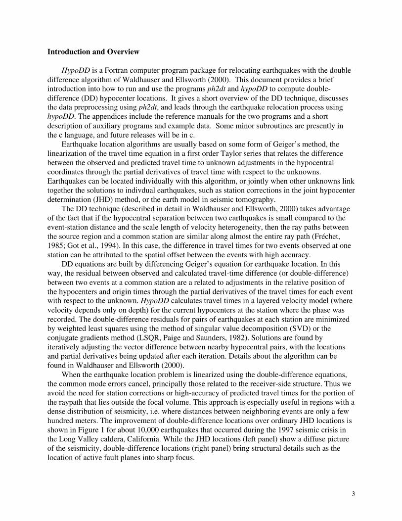
When the earthquake location problem is linearized using the double-difference equations, the common mode errors cancel, principally those related to the receiver-side structure. Thus we avoid the need for station corrections or high-accuracy of predicted travel times for the portion of the raypath that lies outside the focal volume. This approach is especially useful in regions with a dense distribution of seismicity, i.e. where distances between neighboring events are only a few hundred meters. The improvement of double-difference locations over ordinary JHD locations is shown in Figure 1 for about 10,000 earthquakes that occurred during the 1997 seismic crisis in the Long Valley caldera, California. While the JHD locations (left panel) show a diffuse picture of the seismicity, double-difference locations (right panel) bring structural details such as the location of active fault planes into sharp focus.

3

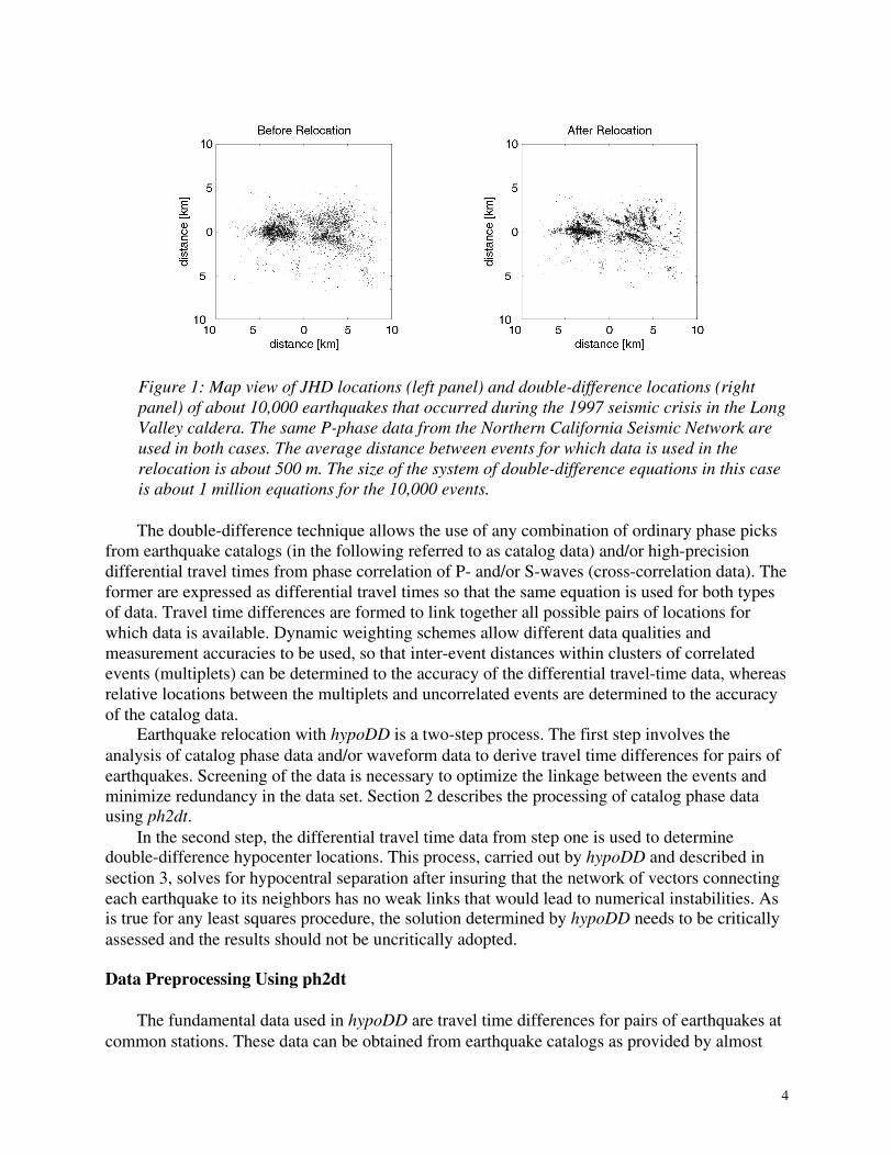
Figure 1: Map view of JHD locations (left panel) and double-difference locations (right panel) of about 10,000 earthquakes that occurred during the 1997 seismic crisis in the Long Valley caldera. The same P-phase data from the Northern California Seismic Network are used in both cases. The average distance between events for which data is used in the relocation is about 500 m. The size of the system of double-difference equations in this case is about 1 million equations for the 10,000 events.

The double-difference technique allows the use of any combination of ordinary phase picks from earthquake catalogs (in the following referred to as catalog data) and/or high-precision differential travel times from phase correlation of P- and/or S-waves (cross-correlation data). The former are expressed as differential travel times so that the same equation is used for both types of data. Travel time differences are formed to link together all possible pairs of locations for which data is available. Dynamic weighting schemes allow different data qualities and measurement accuracies to be used, so that inter-event distances within clusters of correlated events (multiplets) can be determined to the accuracy of the differential travel-time data, whereas relative locations between the multiplets and uncorrelated events are determined to the accuracy of the catalog data.

Earthquake relocation with hypoDD is a two-step process. The first step involves the analysis of catalog phase data and/or waveform data to derive travel time differences for pairs of earthquakes. Screening of the data is necessary to optimize the linkage between the events and minimize redundancy in the data set. Section 2 describes the processing of catalog phase data using ph2dt.

In the second step, the differential travel time data from step one is used to determine double-difference hypocenter locations. This process, carried out by hypoDD and described in section 3, solves for hypocentral separation after insuring that the network of vectors connecting each earthquake to its neighbors has no weak links that would lead to numerical instabilities. As is true for any least squares procedure, the solution determined by hypoDD needs to be critically assessed and the results should not be uncritically adopted.

Data Preprocessing Using ph2dt

The fundamental data used in hypoDD are travel time differences for pairs of earthquakes at common stations. These data can be obtained from earthquake catalogs as provided by almost

4

any seismic network and/or from waveform cross correlation (e.g., Poupinet et al., 1984). In both cases travel time differences for pairs of events are required that ensure stability of the least square solution and optimize connectedness between events. This section describes ph2dt, a program that transforms catalog P- and S-phase data into input files for hypoDD.

Ph2dt searches catalog P- and S-phase data for event pairs with travel time information at common stations and subsamples these data in order to optimize the quality of the phase pairs and the connectivity between the events. Ideally, we seek a network of links between events so that there exists a chain of pairwise connected events from any one event to any other event, with the distance being as small as possible between connected events. Ph2dt establishes such a network by building links from each event to a maximum of MAXNGH neighboring events within a search radius defined by MAXSEP. (The variable names in bold type are listed in appendix A, along with suggested values.) To reach the maximum number of neighbors, only "strong" neighbors are considered, i.e. neighbors linked with more than MINLNK phase pairs. "Weak" neighbors, i.e. neighbors with less than MINLNK phase pairs, are selected but not counted as strong neighbors. A strong link is typically defined by eight or more observations (one observation for each degree of freedom). However, a large number of observations for each event pair do not always guarantee a stable solution, as the solution critically depends on the distribution of the stations, to name one factor.

To find neighboring events the nearest neighbor approach is used. This approach is most appropriate if the events are randomly distributed within the search radius (MAXSEP) (i.e. if the radius is similar to the errors in routine event locations). Other approaches such as Delauney tessellation (Richard-Dinger and Shearer, 2000) might be more appropriate in cases where seismicity is strongly clustered in space over large distances, or errors in initial locations are much smaller than the search radius. The search radius, however, should not exceed a geophysically meaningful value; i.e. the hypocentral separation between two earthquakes should be small compared to the event-station distance and the scale length of the velocity heterogeneity. A radius of about 10 km is an appropriate value to start with in many regions.

Even when considering only a few hundred events, the number of possible double-difference observations (delay times) may become very large. One way to circumvent this problem is to restrict the number of links for each event pair, i.e., defining a minimum and a maximum number of observations to be selected for each event pair (MINOBS and MAXOBS). For a large number of events, one might consider only strongly connected event pairs by setting MINOBS equal to MINLNK. For 10,000 well connected events, for example, ph2dt would typically output about one million delay times with the following parameter setting: MAXNGH = 8, MINLNK = 8, MINOBS = 8, MAXOBS = 50. On the other hand, for a small number of events that form a tight cluster one might select all phase pairs available by setting MINOBS = 1, MAXOBS to the number of stations, and MAXNGH to the number of events.

To control the depth difference between an event pair, a range of vertical slowness values is required. Stations close to an event pair are usually the most effective for controlling the depth offset between the two events. Therefore, ph2dt selects observations from increasingly distant stations until the maximum number of observations per event pair (MAXOBS) is reached. In this process, phase picks with a pick weight smaller than MINWGHT (but larger than 0) are ignored. Again, links of event pairs that have less than MINOBS observations are discarded.

A negative weight is a flag to ph2dt to include these readings regardless of their absolute weight whenever the paired event also has observations of this phase at the particular station. The preprocessing program ncsn2pha (Appendix C) automatically marks reading weights with a

5

negative sign whenever the diagonal element of the data resolution matrix, or Hat matrix (data importance reported by Hypoinverse (Klein, 1989, and personal communication, 2001)) is larger than 0.5. Users without importance information are encouraged to consider preprocessing the input to ph2dt to flag critical station readings. Readings with negative weights are used in addition to the MAXOBS phase pairs with positive weights.

Ph2dt removes observations that are considered as outliers. Outliers are identified as delay times that are larger than the maximum expected delay time for a given event pair. The maximum expected delay time is the time for a P-/S-wave to travel between two events and is calculated from the initial event locations and a P- and S-velocity in the focal area of 4 and 2.3 km/s, respectively. 0.5 seconds are added to the cutoff to account for uncertainty in the initial locations. Outliers are reported in the file ph2dt.log. The outlier detection and removal task is programmed in ph2dt as are the parameters that control it. If necessary, however, it can easely be changed by editing the source code.

After having established the network of event pairs linking together all events, ph2dt reports key values that indicate whether the events are generally well connected or not: the number of weakly linked events, the average number of links per event pair, and the average distance between strongly linked events. The average distance between strongly linked events indicates the density of the hypocenter distribution, and guides on the choice of the maxium hypocenter separation allowed in hypoDD (parameter WDCT, next section).

The grouping of events into clusters of well-connected events (i.e. clusters where the events of one cluster never connect to events of another cluster or only through event pairs that have less than a specific number of observations), however, is explicitly performed in hypoDD to ensure stability of the inversion (see next section). To improve connectedness throughout a cluster of events, the values MAXNGH and/or MINLNK can be increased in ph2dt to reach more distant neighbors for each event, unfortunatly at the cost of introducing model errors during relocation. Increasing MAXNGH generally produces more delay times, while increasing MINLNK

might result in ph2dt not finding MAXNGH neighbors within the search radius. It is recommended to be rather liberal in the selection of data using ph2dt, and to be more restrictive in hypoDD (through OBSCT and WDCT, see next section) if necessary.

To obtain waveform based differential arrival time measurements we refer to various existing techniques (e.g. Poupinet et al., 1984; Dodge, 1996; Schaff et al., 2001). Such data can easily be combined with catalog data in hypoDD, or used on its own. Note, however, that when using cross-correlation differential times, phases may correlate under specific event-pair station configurations only, such as in cases where the event pair offset is small compared to the distance to a common station and focal mechanisms are very similar. Thus, although the measurements may be of high accuracy, the spread of the partial derivatives might not be optimal to control the relative locations of the two events. Inspection of the station distribution prior to relocation is necessary to assess the relocation results.

Important notes: 1) Every earthquake must have a unique id number, otherwise misreferencing and strange behavior will result. 2) When combining catalog and waveform based relative travel time measurements, it is critical that both measurements are referenced to the same event origin times. This is not always the case, as origin times reported in catalogs may be different from the origin times included in the header of the waveform data. In this case, a correction has to be applied (see Appendix B.3.2). Combining both data types also requires appropriate weighting during relocation with hypoDD to account for the different accuracy and error characteristics of the data.

6

Earthquake Relocation Using hypoDD

This section explains how to use hypoDD to determine double-difference hypocenter locations from differential travel time data. It discusses the relocation process and the parameters that control it. For a detailed description of the parameters see appendix B.

Data Selection and Event Clustering

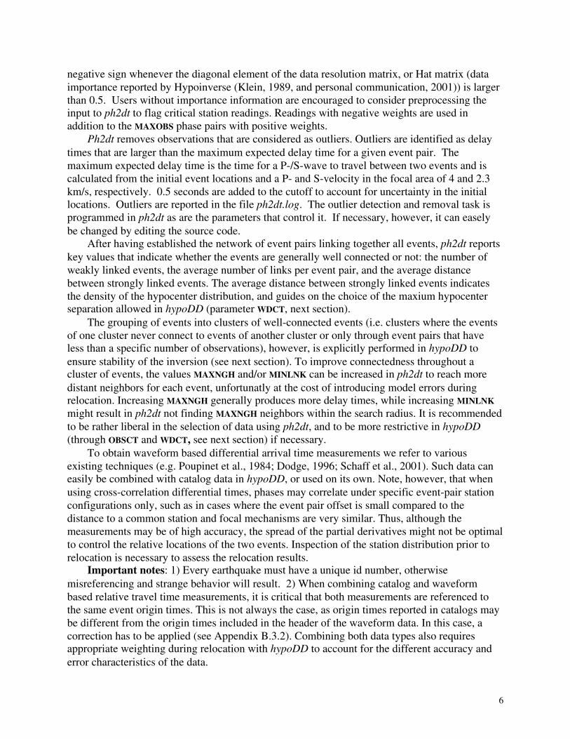
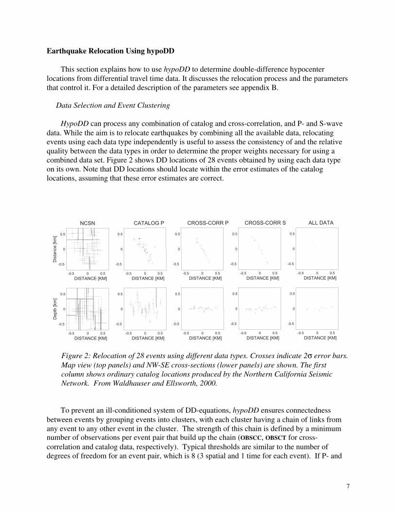
HypoDD can process any combination of catalog and cross-correlation, and P- and S-wave data. While the aim is to relocate earthquakes by combining all the available data, relocating events using each data type independently is useful to assess the consistency of and the relative quality between the data types in order to determine the proper weights necessary for using a combined data set. Figure 2 shows DD locations of 28 events obtained by using each data type on its own. Note that DD locations should locate within the error estimates of the catalog locations, assuming that these error estimates are correct.

Figure 2: Relocation of 28 events using different data types. Crosses indicate 2σ error bars. Map view (top panels) and NW-SE cross-sections (lower panels) are shown. The first column shows ordinary catalog locations produced by the Northern California Seismic Network. From Waldhauser and Ellsworth, 2000.

To prevent an ill-conditioned system of DD-equations, hypoDD ensures connectedness between events by grouping events into clusters, with each cluster having a chain of links from any event to any other event in the cluster. The strength of this chain is defined by a minimum number of observations per event pair that build up the chain (OBSCC, OBSCT for cross-correlation and catalog data, respectively). Typical thresholds are similar to the number of degrees of freedom for an event pair, which is 8 (3 spatial and 1 time for each event). If P- and

7

S-wave data is used, the threshold has to be higher to actually reach 8 stations per event pair. Increasing the threshold might increase the stability of the solution, but it might also split up a large cluster into subclusters. Lowering the threshold might include more events in a single cluster, but might decrease the stability of the solution. A high threshold, however, does not necessarily guarantee stable relocations, as the spread of the partial derivatives is not taken into account directly. Selecting catalog data with ph2dt, however, ensures that the spread is optimized. Note that if the value for OBSCT is larger than the value chosen for MAXOBS in ph2dt when creating the differential time data, then hypoDD will find no clusters (i.e nevent ‘single event clusters’). The value for OBSCT in hypoDD should generally be equal to or less than the value for MINLNK in ph2dt to ensure enough strong links betweens closeby events.

Another factor in hypoDD that controls connectivity between events is the maximum hypocentral separation allowed between linked events. The smaller the maximum separation, the less events will be connected. The parameters that control separation distance in hypoDD are the distance weighting/cutoff parameters WDCT and WDCC (see below). HypoDD removes data for event pairs with separation distances larger than the values given for WDCT and WDCC for the first iteration. Note that the distance cutoff parameter WDCT is similar to the parameter MAXSEP

in ph2dt. It is advised to choose a larger value for MAXSEP in ph2dt and then experiment with smaller values for WDCT in hypoDD to keep separation distances small and still connect all events.

HypoDD reports the clusters with decreasing number of events. If the clusters are known from a previous run of hypoDD, then the parameter CID can be used to relocate an individual cluster. The parameter ID allows you to specify a subset of events out of the event file, such as events that belong to a specific cluster. The clustering task in hypoDD can, as an option, be disabled by setting OBSCC and/or OBSCT to zero. In this mode hypoDD assumes that all events are well connected, and the system of DD equations will not be singular, which may or may not be the case.

Initial Conditions and Solution Control

HypoDD minimizes residuals between observed and calculated travel time differences in an iterative procedure and, after each iteration, updates the locations and partial derivatives, and re-weights the a priori weights of the data according to the misfit during inversion and the offset between the events. Initial locations are taken from the catalog, either at reported locations or at a common location at the centroid of the cluster (under control of ISTART). The centroid option might be appropriate for clusters of small dimensions, and is useful to investigate the effect of variation in initial locations on the solution.

ISOLV allows the choice of two methods to solve the system of DD equations: singular value decomposition (SVD) and the conjugate gradients method (LSQR, Paige & Saunders, 1982). SVD is useful for examining the behavior of small systems (about 100 events depending on available computing capacity) as it provides information on the resolvability of the hypocentral parameters and the amount of information supplied by the data, and adequately represents least squares errors by computing proper covariances. LSQR takes advantage of the sparseness of the system of DD-equations and is able solve a large system efficiently. Errors reported by LSQR, however, are grossly under estimated and need to be assessed independently by using, for example, statistical resampling methods (see Waldhauser and Ellsworth, 2000) or SVD on a subset of events.

8

LSQR solves the damped least squares problem. DAMP is the damping factor that damps the hypocentral adjustments if the adjustment vector becomes large or unstable. The choice for the damping factor strongly depends on the condition of the system to be solved. The condition of the system is expressed by the condition number (see CND in hypoDD standard output and in hypoDD.log), which is the ratio of the largest to smallest eigenvalue. Generally a damping between 1 and 100 is appropriate, resulting in a condition number that is between about 40 and 80 (these are empirical values). If the condition number is higher (lower) damping needs to be increased (decreased). If a very high damping is needed to lower the condition number, or if the condition number remains high, then the DD system might not be well conditioned. This might be because of weak links between events, data outliers, extreme spread of weights, etc. The straightforward way to improve the stability of the inversion is by better constraining the solution: i.e. requiring more links between events through OBSCT /OBSCC (the minimum number of catalog/cross-correlation links per event pair to form a continuous cluster) and/or modifying the weighting and re-weighting scheme. It might also be necessary to go back to ph2dt and generate a differential time data set (the dt.ct output files) that allows for more neighbors for each event (increasing MAXNGH or MINLNK). One could also include more distant events by increasing MAXSEP.

While it is easy to control the performance of hypoDD on a small number of events (by using SVD, for example), it is more difficult to assess the reliablity of the locations in the case of thousands of events that can only be relocated in LSQR mode. Larger numbers of earthquakes generally produce larger condition numbers, as it only takes one poorly constrained event to drive up the condition number. One test case with 1000 events and damping values of 20, 40 and 60 yielded condition numbers of 450, 180 and 100, with a comparable RMS residual reduction for each case. While the internal structure of the relocated seismicity is generally similar for results with different condition numbers, the absolute location of the structures might strongly depend on the inversion parameters. A solution should be found where the change in absolute centroid location is within the average error of the initial locations.

The damping of the solution vector allows some control of how fast a solution converges, which affects the choice of the number of iterations (NITER). In general, the first few iterations contribute the most to the shifts in hypocenter locations. Typically the mean shift after the first few iterations is on the order of the uncertainty in the catalog locations. Iteration can be stopped when the shifts in hypocenter adjustments and/or the RMS residual dropped below the noise level of the data.

The number of events before and after relocation might not be same. Events get deleted if they completely lose linkage as a result of the reweighting (see below). Also, during the iteration process some events try to become airquakes -- hypocenters that locate above the ground after relocation. Airquakes occur when event pairs locate near the surface, and the control in vertical offset between the events is poor. This problem can be addressed by increasing damping (to prevent solution fluctuations), or by improving the geometrical control by including more stations close to the event pair. Also, a near surface velocity that is higher than the true velocity pushes hypocenters up, while a lower than true velocity pushes hypocenters down. HypoDD removes air quakes after each iteration, repeating the previous iteration without the air quakes.

As in the absolute location problem, the main limitation of the DD technique is the availability and distribution of stations. Special attention has to be given in cases where there are only a few stations within a focal depth. In such cases, the station geometry fundamentally limits what we can do to relocate the events. This is particularly true for cases where the nearest station

9

is a leverage point of the solution, thus making it impossible to detect when its readings are bad.

Data Weighting and Re-weighting

One aspect of weighting is the original weights assigned each phase in the catalog. The weight code 0 implies a weight of 1.0, 1 implies 0.5, 2 implies 0.2, 3 implies 0.1, and 4-9 imply 0.0. This weight translation is done by the program ncsn2pha, and weights are used both in the relocation in hypoDD and to screen out phases not to be associated in ph2dt and hypoDD.

The weighting and re-weighting of the data is a crucial part of the relocation process. The general choice of a priori weights (WTCCP, WTCCS, WTCTP, WTCTS, the weights for the four data types) and the characteristics of the re-weighting functions (WRCC, WRCT, WDCC, WDCT, controls the cutoff of outlier data) are described in Waldhauser and Ellsworth (2000). Here we show a more complicated case to demonstrate the choice of a proper weighting scheme. Figure 3 shows about 250 events for which catalog and cross correlation P- and S-wave data are available. Routine locations show two clusters at different depths, each representing a diffuse cloud of events (top row, left). Note the event in the deeper cluster marked by an ‘+’.

Relocations using only catalog data (top row, middle) show a tighter clustering of the events within each of the two clusters, relative to the initial locations. The ‘+’ event moved upwards midway between the two clusters. Relocations using only cross-correlation data (top row, right) show a collapsing of the events into groups of repeating earthquake sequences, where events lie virtually on top of each other. Note that the ‘+’ event appears to belong to such a repeating earthquake sequence in the upper cluster. Compared to the routine locations the shallower cluster moved down while the deeper cluster moved up, resulting in a smaller vertical offset between the two clusters. While the seismicity structure within the clusters appear to be adequately imaged, the relative location between the two clusters seems to be uncertain. Inspection of the station distribution for the event pairs that connect the two clusters over large distances reveal that waveforms did not correlate at stations close to the event pairs (due to the stronger influence of the structure for these stations), leading to a lack of vertical control. In order to properly combine the two data sets, strong weights need to be given to catalog data of event pairs with large separation distances, and strong weights for cross-correlation data for event pairs with small separation distances. Such a weighting scheme is given in Table 1. We first perform 5 iterations during which we (a priori) down-weight the cross correlation data in order to allow the catalog data to restore the large-scale picture. During iterations 6-10 we keep the same relative a priori weights, but re-weight the catalog data according to misfit and event separation to remove or down-weight outliers. At iteration 10 the locations of the events are primarily controlled by the catalog data (middle row, left). During the following iterations (11-25) we improve the locations of events whose waveforms correlate by down-weighting the catalog data relative to the cross-correlation data. To assure that the large separation distances are still controlled by the catalog data, we allow the cross- correlation data to constrain only event pairs with separations smaller than 2 km (iterations 11-20). No misfit dependant weight is applied to the cross correlation data during iterations 11-15 (middle row, center), but is applied during iterations 16-20 (middle row, right). Note that the ‘+’ event moved to the repeating earthquake sequence in the upper cluster (see expanded view in bottom row). The final 5 iterations (21-25) primarily use cross-correlation data of event pairs that separate less than 500 m to resolve the structure at the scale of individual earthquakes.

10

Figure 3: Relocation of events using different data types (top row of panels). Middle row shows locations during different stages in the iteration process using the combined set of data and the weighting scheme shown in Table 1. Bottom row shows detailed views of the upper cluster of earthquakes shown in the middle panels. Note the location of the event marked with a ‘+’. Circles represent rupture areas for a 30 bar constant stress drop model.

Table 1: Weighting scheme for data in Figure 3.

Cross correlation data Catalog data

Iterations A priori, P-wave A priori, S-wave Misfit weight Dist. Weight A priori, P-wave A priori, S-wave Misfit weight Dist. Weigh

WTCCP WTCCS (residual cutoff, (seperation in WTCTP WTCTS (residual cutoff, (seperation in factor times SD) km) factor times SD) km)

WRCC WDCC WRCT WDCT

1-5 0.01 0.01 -9 -9 1.0 0.5 -9 -9

6-10 0.01 0.01 -9 -9 1.0 0.5 6 4

11-15 1.0 0.5 -9 2 0.01 0.005 6 4

16-20 1.0 0.5 6 2 0.01 0.005 6 4

21-25 1.0 0.5 6 0.5 0.01 0.005 6 4

11

The iteration-dependent weights in table1, and the capitalized variable names, correspond exactly to variables specified in the hypoDD input parameter file hypoDD.inp. See Appendix B.3.1 for an example. A value of –9 means that the weighting of that type is not used on that iteration, corresponding to a very large value of event separation in km or large misfit in seconds.

Analysis of hypoDD Output

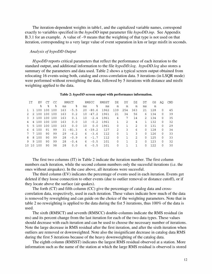
HypoDD reports critical parameters that reflect the performance of each iteration to the standard output, and additional information to the file hypoDD.log. hypoDD.log also stores a summary of the parameters and data used. Table 2 shows a typical screen output obtained from relocating 16 events using both, catalog and cross-correlation data. 5 iterations (in LSQR mode) were performed without reweighting the data, followed by 5 iterations with distance and misfit weighting applied to the data.

Table 2: hypoDD screen output with performance information.

IT EV CT CC RMSCT RMSCC RMSST DX DY DZ DT OS AQ CND % % % ms % ms % ms m m m ms m

1 1 100 100 100 163 -5.5 20 -80.6 1962 139 254 363 21 128 0 45 2 2 100 100 100 163 0.2 10 -47.2 1961 21 34 56 6 134 0 39 3 3 100 100 100 163 0.1 10 -2.4 1961 4 7 14 2 134 0 35 4 4 100 100 100 163 0.0 10 -0.2 1961 1 2 4 1 132 0 32 5 5 100 100 100 163 0.0 10 0.0 1961 0 1 2 0 131 0 29 6 6 100 91 99 31 -81.3 6 -39.2 127 2 3 6 0 128 0 34 7 7 100 90 99 29 -6.2 6 -3.6 112 0 1 3 0 126 0 33 8 8 100 90 99 28 -0.9 6 -1.7 112 0 1 2 0 125 0 33 9 9 100 90 99 28 -0.4 6 -0.5 101 0 1 2 0 123 0 32

10 10 100 90 98 28 0.0 6 -0.5 101 0 1 1 0 122 0 30

The first two columns (IT) in Table 2 indicate the iteration number. The first column numbers each iteration, while the second column numbers only the sucessful iterations (i.e. the ones without airquakes). In the case above, all iterations were sucessful.

The third column (EV) indicates the percentage of events used in each iteration. Events get deleted if they loose connection to other events (due to outlier removal or distance cutoff), or if they locate above the surface (air quakes).

The forth (CT) and fifth column (CC) give the percentage of catalog data and cross-correlation data, respectively, used in each iteration. These values indicate how much of the data is removed by reweighting and can guide on the choice of the weighting parameters. Note that in table 2 no reweighting is applied to the data during the fist 5 iterations, thus 100% of the data is used.

The sixth (RMSCT) and seventh (RMSCC) double-columns indicate the RMS residual (in ms) and its percent change from the last iteration for each of the two data types. These values should decrease with each iteration and can be used to choose the necessary number of iterations. Note the large decrease in RMS residual after the first iteration, and after the sixth iteration when outliers are removed or downweighted. Note also the insignificant decrease in catalog data RMS during the first 5 iterations because of the heavy downweighting of the catalog data.

The eighth column (RMSST) indicates the largest RMS residual observed at a station. More information such as the name of the station at which the large RMS residual is observed is stored

12

in hypoDD.log. Columns nine to twelve (DX, DY, DZ, DT) indicate the average absolute value of the

change in hypocenter location and origin time during each iteration. Changes during the first iterations should be in the range of the uncertainty of the initial (catalog) locations (assuming that these are correct). They should continously decrease until they are within the noise level of the data. If hypoDD runs in LSQR mode, too small or too large changes may indicate that the solution is overdamped (damping value is to high) or underdamped (damping value is too low).

Column thirteen (OS) indicates the absolute shift in cluster origin, i.e. the shift between the cluster centroid of the initial locations and the cluster centroid of the relocations. Only the largest value of the 3 spatial directions is given - more information can be found in hypoDD.log. Absolute shifts of the cluster centroid are unconstrained and should be small, preferably smaller than the average error in the initial locations.

Column forteen (AQ) indicates the number of air earthquakes detected and discarded (see section 3). Note that a large number of air-quakes might indicate a damping value that is too small or an inapropriate velocity model. Iterations with air-quakes will be repeated with the air-quakes removed.

The last column (CND) indicates the condition number for the system of double-difference equations (i.e. the ratio between the largest and smallest eigenvalue; see section 3). A low value may indicate overdamping of the solution, a high value underdamping. Generally, a condition number between 40 and 80 has been shown to be appropriate. Note that the CND column is omitted when hypoDD runs in SVD mode.

Error Assessment

Careful attention has to be addressed to the final output of hypoDD. Error estimates assigned to the relocated hypocenters need to be reviewed (in particular when the solution is found with LSQR), and the robustness of the relocation results needs to be tested. This is especially important when the station distribution is sparse and/or azimuthal coverage of available phases is not optimal. Different techniques to assess the error estimates reported by hypoDD are described in Waldhauser and Ellsworth (2000). Such techniques include, but are not limited to, tests against changes in station distribution (e.g. resampling of the data by deleting one station at the time), changes in the velocity model, changes the initial hypocenter locations (e.g. through ISTART), or changes in the number of events (resampling of the data by deleting one event at the time). LSQR results need to be reviewed by relocating subsets of events using SVD to get proper least squares error estimates.

The hypoDD program package comes with several example data files (see Appendix D) of various size and type together with input control parameter files for ph2dt and hypoDD. Format conversion programs are available to reformat commonly used data formats (see Appendix C).

References

Dodge, D. (1996), Microearthquake studies using cross-correlation derived hypocenters, Ph.D. thesis, Stanford University, 146pp.

Fréchet, J. (1985), Sismogenèse et doublets sismiques, Thèse d’Etat, Université Scientifique et Médicale de Grenoble, 206 pp.

13

Got, J.-L., J. Fréchet and F.W. Klein (1994), Deep fault plane geometry inferred from multiplet relative relocation beneath the south flank of Kilauea, J. Geophys. R. 99, 15375-15386.

Klein, F.W. (1989), User’s Guide to HYPOINVERSE, a program for VAX computers to solve for earthquake locations and magnitude, U.S.G.S. open-file report 89-314.

Paige, C.C. and M.A. Saunders (1982), LSQR: Sparse linear equations and least squares problems, ACM Transactions on Mathematical Software 8/2, 195-209.

Poupinet, G., W.L. Ellsworth, and J. Fréchet (1984), Monitoring velocity variations in the crust using earthquake doublets: an application to the Calaveras fault, California, J. Geophys. R. 89, 5719-5731.

Richards-Dinger, K.B. and P.M. Shearer (2000), Earthquake locations in southern California obtained using source-specific station terms, J. Geophys. R. 105, 10939-10960.

Schaff, D.P., G.H.R. Bokelmann, G.C. Beroza, E. Zanzerika, W.L. Ellsworth, and F. Waldhauser (2001), Cross-correlation arrival time measurement for earthquake location, to be submitted to J. Geophys. R.

Waldhauser, F. and W.L. Ellsworth, A double-difference earthquake location algorithm: Method and application to the northern Hayward fault, Bull. Seismol. Soc. Am., 90, 1353-1368, 2000.

Acknowledgements

The help of many people that tested and used hypoDD and reported errors and provided me with invaluable suggestions to improve the code is greatly acknowledged: Greg Beroza, Goetz Bokelmann, John Cassidy, Alex Cole, Bill Ellsworth, Bruce Julian, Fred Klein, Andy Michael, David Oppenheimer, Stephanie Prejean, Keith Richards-Dinger, Stephanie Ross, David Schaff, and Eva Zanzerkia. Special thanks go to Bruce Julian, Keith Richards-Dinger, and Fred Klein for their work on testing and cleaning up the code and putting it under RCS. Fred Klein and Bill Ellsworth are thanked for the numerous comments and suggestions that greatly improved this document. Fred Klein and David Schaff are thanked for providing the test data sets 1-3 and the cross correlation data in example 2, respectively.

14

APPENDIX A. Reference for ph2dt

A.1 Description

Conversion of phase data from earthquake catalogs to travel time differences for pairs of earthquakes at common stations. Output files are input files to hypoDD.

A.2 Installation and Syntax

ph2dt is written in Fortran77 and is currently running on a Sun/Unix platform under Solaris and on PC/Mac under Linux. Execute the Makefile to compile and load the program. Change array dimensions in ph2dt.inc in the include directory according to the size of the problem to be solved and the capacity of the computer.

Syntax to run the program: ph2dt [controlfile]

for input of control parameters via control file or ph2dt <ret>

for interactive input.

A.3 Input Files

A.3.1 Control File (e.g. file ph2dt.inp)

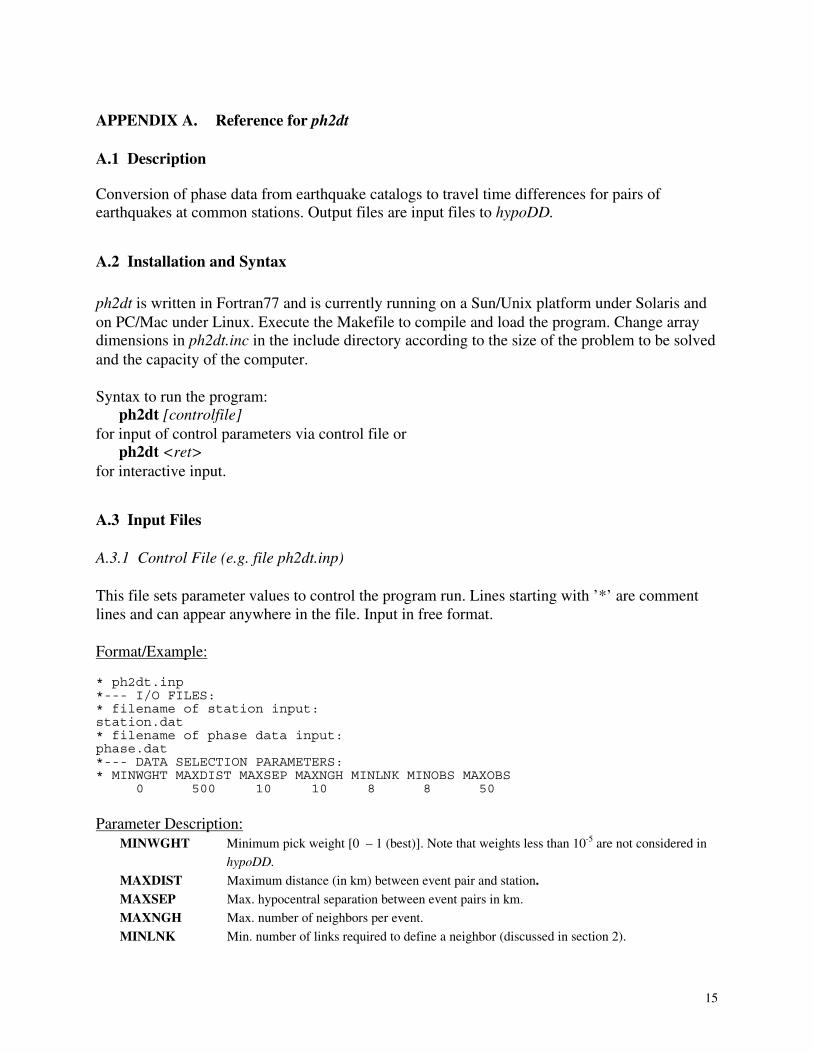
This file sets parameter values to control the program run. Lines starting with ’*’ are comment lines and can appear anywhere in the file. Input in free format.

Format/Example:

* ph2dt.inp *--- I/O FILES: * filename of station input: station.dat * filename of phase data input: phase.dat *--- DATA SELECTION PARAMETERS: * MINWGHT MAXDIST MAXSEP MAXNGH MINLNK MINOBS MAXOBS

0 500 10 10 8 8 50

Parameter Description: MINWGHT Minimum pick weight [0 – 1 (best)]. Note that weights less than 10-5 are not considered in

hypoDD.

MAXDIST Maximum distance (in km) between event pair and station. MAXSEP Max. hypocentral separation between event pairs in km.

MAXNGH Max. number of neighbors per event.

MINLNK Min. number of links required to define a neighbor (discussed in section 2).

15

MINOBS Min. number of links per pair saved.

MAXOBS Max. number of links per pair saved (ordered by distance from event pair).

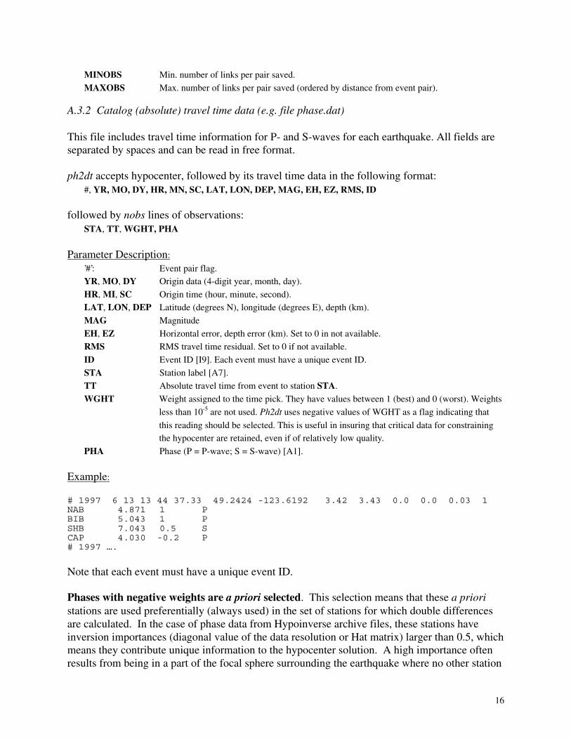
A.3.2 Catalog (absolute) travel time data (e.g. file phase.dat)

This file includes travel time information for P- and S-waves for each earthquake. All fields are separated by spaces and can be read in free format.

ph2dt accepts hypocenter, followed by its travel time data in the following format: #, YR, MO, DY, HR, MN, SC, LAT, LON, DEP, MAG, EH, EZ, RMS, ID

followed by nobs lines of observations: STA, TT, WGHT, PHA

Parameter Description:

’#’: Event pair flag. YR, MO, DY Origin data (4-digit year, month, day).

HR, MI, SC Origin time (hour, minute, second).

LAT, LON, DEP Latitude (degrees N), longitude (degrees E), depth (km).

MAG Magnitude

EH, EZ Horizontal error, depth error (km). Set to 0 in not available.

RMS RMS travel time residual. Set to 0 if not available.

ID Event ID [I9]. Each event must have a unique event ID.

STA Station label [A7].

TT Absolute travel time from event to station STA.

WGHT Weight assigned to the time pick. They have values between 1 (best) and 0 (worst). Weights

less than 10-5 are not used. Ph2dt uses negative values of WGHT as a flag indicating that

this reading should be selected. This is useful in insuring that critical data for constraining the hypocenter are retained, even if of relatively low quality.

PHA Phase (P = P-wave; S = S-wave) [A1].

Example:

# 1997 6 13 13 44 37.33 49.2424 -123.6192 3.42 3.43 0.0 0.0 0.03 1 NAB 4.871 1 P BIB 5.043 1 P SHB 7.043 0.5 S CAP 4.030 -0.2 P # 1997 ….

Note that each event must have a unique event ID.

Phases with negative weights are a priori selected. This selection means that these a priori stations are used preferentially (always used) in the set of stations for which double differences are calculated. In the case of phase data from Hypoinverse archive files, these stations have inversion importances (diagonal value of the data resolution or Hat matrix) larger than 0.5, which means they contribute unique information to the hypocenter solution. A high importance often results from being in a part of the focal sphere surrounding the earthquake where no other station

16

is located.

A.3.3 Station location information (e.g. file station.dat)

See Section B.3.5.

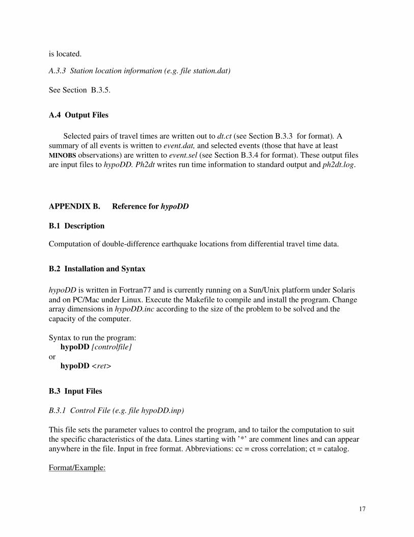
A.4 Output Files

Selected pairs of travel times are written out to dt.ct (see Section B.3.3 for format). A summary of all events is written to event.dat, and selected events (those that have at least MINOBS observations) are written to event.sel (see Section B.3.4 for format). These output files are input files to hypoDD. Ph2dt writes run time information to standard output and ph2dt.log.

APPENDIX B. Reference for hypoDD

B.1 Description

Computation of double-difference earthquake locations from differential travel time data.

B.2 Installation and Syntax

hypoDD is written in Fortran77 and is currently running on a Sun/Unix platform under Solaris and on PC/Mac under Linux. Execute the Makefile to compile and install the program. Change array dimensions in hypoDD.inc according to the size of the problem to be solved and the capacity of the computer.

Syntax to run the program: hypoDD [controlfile]

or hypoDD <ret>

B.3 Input Files

B.3.1 Control File (e.g. file hypoDD.inp)

This file sets the parameter values to control the program, and to tailor the computation to suit the specific characteristics of the data. Lines starting with ’*’ are comment lines and can appear anywhere in the file. Input in free format. Abbreviations: cc = cross correlation; ct = catalog.

Format/Example:

17

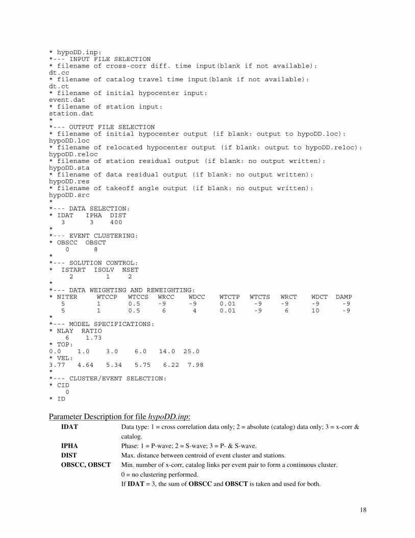
* hypoDD.inp: *--- INPUT FILE SELECTION * filename of cross-corr diff. time input(blank if not available): dt.cc * filename of catalog travel time input(blank if not available): dt.ct * filename of initial hypocenter input: event.dat * filename of station input: station.dat * *--- OUTPUT FILE SELECTION * filename of initial hypocenter output (if blank: output to hypoDD.loc): hypoDD.loc * filename of relocated hypocenter output (if blank: output to hypoDD.reloc): hypoDD.reloc * filename of station residual output (if blank: no output written): hypoDD.sta * filename of data residual output (if blank: no output written): hypoDD.res * filename of takeoff angle output (if blank: no output written): hypoDD.src * *--- DATA SELECTION: * IDAT IPHA DIST

3 3 400 * *--- EVENT CLUSTERING: * OBSCC OBSCT

0 8 * *--- SOLUTION CONTROL: * ISTART ISOLV NSET

2 1 2 * *--- DATA WEIGHTING AND REWEIGHTING: * NITER WTCCP WTCCS WRCC WDCC WTCTP WTCTS WRCT WDCT DAMP

5 1 0.5 -9 -9 0.01 -9 -9 -9 -9 5 1 0.5 6 4 0.01 -9 6 10 -9

* *--- MODEL SPECIFICATIONS: * NLAY RATIO

6 1.73 * TOP: 0.0 1.0 3.0 6.0 14.0 25.0 * VEL: 3.77 4.64 5.34 5.75 6.22 7.98 * *--- CLUSTER/EVENT SELECTION: * CID

0 * ID

Parameter Description for file hypoDD.inp: IDAT Data type: 1 = cross correlation data only; 2 = absolute (catalog) data only; 3 = x-corr &

catalog. IPHA Phase: 1 = P-wave; 2 = S-wave; 3 = P- & S-wave.

DIST Max. distance between centroid of event cluster and stations.

OBSCC, OBSCT Min. number of x-corr, catalog links per event pair to form a continuous cluster.

0 = no clustering performed. If IDAT = 3, the sum of OBSCC and OBSCT is taken and used for both.

18

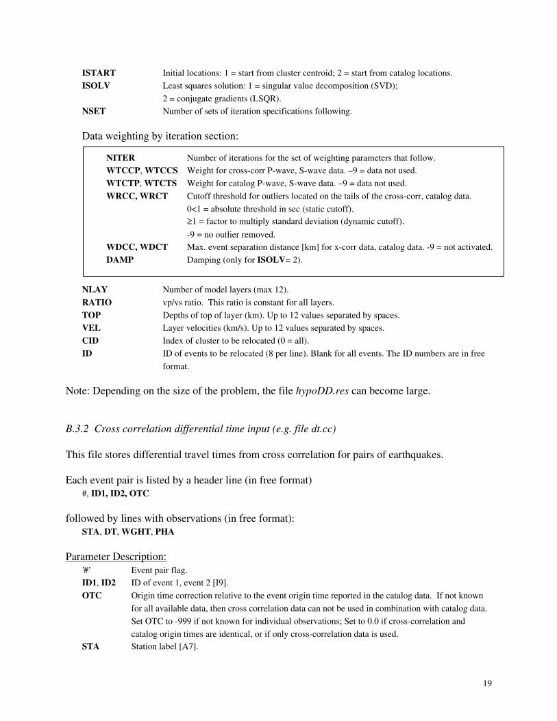
ISTART Initial locations: 1 = start from cluster centroid; 2 = start from catalog locations.

ISOLV Least squares solution: 1 = singular value decomposition (SVD);

2 = conjugate gradients (LSQR). NSET Number of sets of iteration specifications following.

Data weighting by iteration section:

NITER Number of iterations for the set of weighting parameters that follow.

WTCCP, WTCCS Weight for cross-corr P-wave, S-wave data. –9 = data not used.

WTCTP, WTCTS Weight for catalog P-wave, S-wave data. –9 = data not used.

WRCC, WRCT Cutoff threshold for outliers located on the tails of the cross-corr, catalog data.

0<1 = absolute threshold in sec (static cutoff). ≥1 = factor to multiply standard deviation (dynamic cutoff).

-9 = no outlier removed. WDCC, WDCT Max. event separation distance [km] for x-corr data, catalog data. -9 = not activated.

DAMP Damping (only for ISOLV= 2).

NLAY Number of model layers (max 12).

RATIO vp/vs ratio. This ratio is constant for all layers.

TOP Depths of top of layer (km). Up to 12 values separated by spaces.

VEL Layer velocities (km/s). Up to 12 values separated by spaces.

CID Index of cluster to be relocated (0 = all).

ID ID of events to be relocated (8 per line). Blank for all events. The ID numbers are in free

format.

Note: Depending on the size of the problem, the file hypoDD.res can become large.

B.3.2 Cross correlation differential time input (e.g. file dt.cc)

This file stores differential travel times from cross correlation for pairs of earthquakes.

Each event pair is listed by a header line (in free format) #, ID1, ID2, OTC

followed by lines with observations (in free format): STA, DT, WGHT, PHA

Parameter Description: ’#’ Event pair flag. ID1, ID2 ID of event 1, event 2 [I9].

OTC Origin time correction relative to the event origin time reported in the catalog data. If not known

for all available data, then cross correlation data can not be used in combination with catalog data.

Set OTC to -999 if not known for individual observations; Set to 0.0 if cross-correlation and

catalog origin times are identical, or if only cross-correlation data is used. STA Station label [A7].

19

DT Differential time (s) between event 1 and event 2 at station STA. DT = T1-T2.

WGHT Weight of measurement (0 -1; e.g. squared coherency).

PHA Phase (P = P-wave; S = S-wave) [A1]

B.3.3 Catalog travel time input (e.g. file dt.ct)

This file stores absolute travel times from earthquake catalogs for pairs of earthquakes.

Each event pair is listed by a header line (in free format) #, ID1, ID2

followed by nobs lines of observations (in free format): STA, TT1, TT2, WGHT, PHA

Parameter Description: ’#’: Event pair flag. ID1, ID2 ID of event 1, event 2 [I11].

STA Station label [A7].

TT1, TT2 Absolute travel time from event 1, event 2 to station STA.

WGHT Weight of the time pick (0-1).

PHA Phase (P = P-wave; S = S-wave) [A1].

B.3.4 Initial hypocenter input (e.g. file event.dat)

This file stores the initial hypocenter locations. Lines are written in fixed format by the program ph2dt. This makes locating fields such as parts of the date and time easier. Lines are read in free format by hypoDD, however.

One event per line:DATE, TIME, LAT, LON, DEP, MAG, EH, EV, RMS, ID

Parameter Description: DATE Concatenated origin date (YYYYMMDD; year, month and day).

TIME Concatenated origin time (HHMMSSSS; hour, minute and seconds).

LAT, LON, DEP Latitude, longitude, depth (km).

MAG Magnitude (set to 0.0 if not available).

EH, EV Horizontal and vertical error (km) of original location (set to 0.0 if not available).

RMS Residual rms (s) (set to 0.0 is not available).

ID Event identification [I9].

B.3.5 Station input (e.g. station.dat)

This file stores station location information. File is in free format.

One station per line, in either 1) decimal degree format: STA, LAT, LON

20

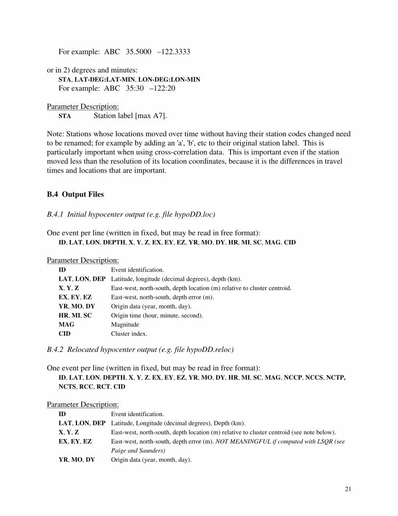
For example: ABC 35.5000 –122.3333

or in 2) degrees and minutes: STA, LAT-DEG:LAT-MIN, LON-DEG:LON-MIN For example: ABC 35:30 –122:20

Parameter Description: STA Station label [max A7].

Note: Stations whose locations moved over time without having their station codes changed need to be renamed; for example by adding an 'a', 'b', etc to their original station label. This is particularly important when using cross-correlation data. This is important even if the station moved less than the resolution of its location coordinates, because it is the differences in travel times and locations that are important.

B.4 Output Files

B.4.1 Initial hypocenter output (e.g. file hypoDD.loc)

One event per line (written in fixed, but may be read in free format): ID, LAT, LON, DEPTH, X, Y, Z, EX, EY, EZ, YR, MO, DY, HR, MI, SC, MAG, CID

Parameter Description: ID Event identification.

LAT, LON, DEP Latitude, longitude (decimal degrees), depth (km).

X, Y, Z East-west, north-south, depth location (m) relative to cluster centroid.

EX, EY, EZ East-west, north-south, depth error (m).

YR, MO, DY Origin data (year, month, day).

HR, MI, SC Origin time (hour, minute, second).

MAG Magnitude

CID Cluster index.

B.4.2 Relocated hypocenter output (e.g. file hypoDD.reloc)

One event per line (written in fixed, but may be read in free format): ID, LAT, LON, DEPTH, X, Y, Z, EX, EY, EZ, YR, MO, DY, HR, MI, SC, MAG, NCCP, NCCS, NCTP, NCTS, RCC, RCT, CID

Parameter Description: ID Event identification.

LAT, LON, DEP Latitude, Longitude (decimal degrees), Depth (km).

X, Y, Z East-west, north-south, depth location (m) relative to cluster centroid (see note below).

EX, EY, EZ East-west, north-south, depth error (m). NOT MEANINGFUL if computed with LSQR (see

Paige and Saunders)

YR, MO, DY Origin data (year, month, day).

21

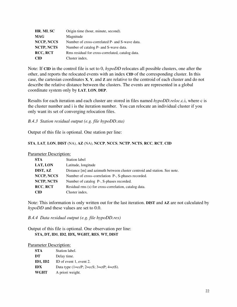
HR, MI, SC Origin time (hour, minute, second).

MAG Magnitude

NCCP, NCCS Number of cross-correlated P- and S-wave data.

NCTP, NCTS Number of catalog P- and S-wave data.

RCC, RCT Rms residual for cross-correlated, catalog data.

CID Cluster index.

Note: If CID in the control file is set to 0, hypoDD relocates all possible clusters, one after the other, and reports the relocated events with an index CID of the corresponding cluster. In this case, the cartesian coordinates X, Y, and Z are relative to the centroid of each cluster and do not describe the relative distance between the clusters. The events are represented in a global coordinate system only by LAT, LON, DEP.

Results for each iteration and each cluster are stored in files named hypoDD.reloc.c.i, where c is the cluster number and i is the iteration number. You can relocate an individual cluster if you only want its set of converging relocation files.

B.4.3 Station residual output (e.g. file hypoDD.sta)

Output of this file is optional. One station per line:

STA, LAT, LON, DIST (NA), AZ (NA), NCCP, NCCS, NCTP, NCTS, RCC, RCT, CID

Parameter Description: STA Station label

LAT, LON Latitude, longitude

DIST, AZ Distance [m] and azimuth between cluster centroid and station. See note.

NCCP, NCCS Number of cross–correlation P-, S-phases recorded.

NCTP, NCTS Number of catalog P-, S-phases recorded.

RCC, RCT Residual rms (s) for cross-correlation, catalog data.

CID Cluster index.

Note: This information is only written out for the last iteration. DIST and AZ are not calculated by hypoDD and these values are set to 0.0.

B.4.4 Data residual output (e.g. file hypoDD.res)

Output of this file is optional. One observation per line: STA, DT, ID1, ID2, IDX, WGHT, RES, WT, DIST

Parameter Description: STA Station label.

DT Delay time.

ID1, ID2 ID of event 1, event 2.

IDX Data type (1=ccP; 2=ccS; 3=ctP; 4=ctS).

WGHT A priori weight.

22

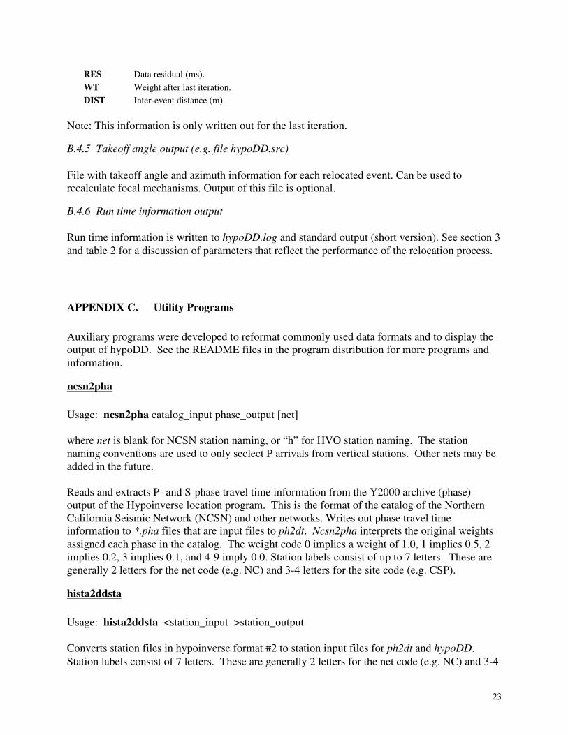
RES Data residual (ms).

WT Weight after last iteration.

DIST Inter-event distance (m).

Note: This information is only written out for the last iteration.

B.4.5 Takeoff angle output (e.g. file hypoDD.src)

File with takeoff angle and azimuth information for each relocated event. Can be used to recalculate focal mechanisms. Output of this file is optional.

B.4.6 Run time information output

Run time information is written to hypoDD.log and standard output (short version). See section 3 and table 2 for a discussion of parameters that reflect the performance of the relocation process.

APPENDIX C. Utility Programs

Auxiliary programs were developed to reformat commonly used data formats and to display the output of hypoDD. See the README files in the program distribution for more programs and information.

ncsn2pha

Usage: ncsn2pha catalog_input phase_output [net]

where net is blank for NCSN station naming, or “h” for HVO station naming. The station naming conventions are used to only seclect P arrivals from vertical stations. Other nets may be added in the future.

Reads and extracts P- and S-phase travel time information from the Y2000 archive (phase) output of the Hypoinverse location program. This is the format of the catalog of the Northern California Seismic Network (NCSN) and other networks. Writes out phase travel time information to *.pha files that are input files to ph2dt. Ncsn2pha interprets the original weights assigned each phase in the catalog. The weight code 0 implies a weight of 1.0, 1 implies 0.5, 2 implies 0.2, 3 implies 0.1, and 4-9 imply 0.0. Station labels consist of up to 7 letters. These are generally 2 letters for the net code (e.g. NC) and 3-4 letters for the site code (e.g. CSP).

hista2ddsta

Usage: hista2ddsta <station_input >station_output

Converts station files in hypoinverse format #2 to station input files for ph2dt and hypoDD. Station labels consist of 7 letters. These are generally 2 letters for the net code (e.g. NC) and 3-4

23

letters for the site code (e.g. CSP). Catalog station codes also have a component/channel code (typically 3 letters) that is not needed here because times from all components can be used and compared with times from all other components. This program acts as a unix filter and needs “< >” symbols for file naming.

eqplot.m

Matlab script to display the hypoDD output files hypoDD.reloc, hypoDD.loc, hypoDD.sta. Type eqplot in a Matlab window in the directory that contains the files. Parameters to make changes to the plot can be edited at the beginning of the script.

APPENDIX D. Example Data

The hypoDD program package comes with several example data files that can be used to learn how to run the programs and test that the users implementation gives the same results as the original USGS version (see README files for instructions). Each example has its own directory, and each directory contains some or all of the following files:

Readme - Comments about this test set. ***.sum - earthquake location summary file in Hypoinverse format ***.arc - earthquake phase/archive file in Hypoinverse format (input to ncsn2pha) ***.pha - hypoDD format phase file (from ncsn2pha, input to ph2dt) ***.ps - map and cross section plots of initial and relocated events ph2dt.inp - ph2dt control parameters (input to ph2dt) station.dat - station locations (input to ph2dt and hypoDD) ph2dt.log - ph2dt run time information (output of ph2dt) dt.ct - catalog travel time differences (output of ph2dt; input to hypoDD) dt.cc - cross-correlation differential times (input for hypoDD) event.dat - initial hypocenter locations (output of ph2dt; input to hypoDD) event.sel - selected initial hypocenter locations (output of ph2dt; input to hypoDD) hypoDD.inp - hypoDD control parameters (input to hypoDD) hypoDD.loc - initial hypocenter locations (output of hypoDD) hypoDD.reloc - relocated hypocenter locations (output of hypoDD) hypoDD.reloc.c.i - intermediate relocations from cluster c and iteration i hypoDD.sta - station residuals (output of hypoDD) hypoDD.log - hypoDD run time information (output of hypoDD) ***.command - sample unix command files used to run the programs terminal.output.ph2dt - output sent to the screen from ph2dtterminal.output.hypoDD - output sent to the screen from hypoDD

Note: The files .pha were formed from travel time information provided by the NCSN catalog. Some examples also have the original NCSN catalog files (*.arc), which can be transformed with ncsn2pha (see Appendix C) to obtain the *.pha file.

The output files of hypoDD can be viewed with the enclosed Matlab script eqplot.m (see Appendix C). hypoDD format files can also be plotted with the QPLOT plotting program (Fred

24

Klein, personal communication). The number of events carried through the processing generally diminishes slightly as they

are ejected for various reasons including being too far outside a cluster to link up with it, or attempting to locate above the ground surface. The number of events quoted below in the number in hypoDD.loc, the number considered relocatable going into hypoDD. The examples include, but are not limited to the following earthquake data sets:

Example 1 - small catalog and c-c set A small set of 16 earthquakes from a “streak” structure on the Hayward Fault near Berkeley. The data are both cross-correlation and catalog. See the Readme files for more information.

Example 2 - catalog and c-c set A set of 308 earthquakes from a section of the Calaveras Fault. The data are both cross-correlation and catalog P- and S-wave data for the period 1984-1999. See the Readme files for more information.

Example 3 - large catalog set A set of ~10000 earthquakes from the Long Valley caldera. The data are catalog P- and S-wave data for seismic activity in 1997. See the Readme files for more information.

Test 1 - large catalog set A large set of 12292 earthquakes from a small square near the juncture of the San Andreas and Calaveras Faults. The data are catalog only for the period 1984-2000. See the Readme files for more information.

Test 2 - small catalog set A small set of 1014 earthquakes from the same small square near the juncture of the San Andreas and Calaveras Faults. The data are a subset of test1 for the period 1999-2000. See the Readme files for more information.

Test 3 - large catalog set A large set of 8281 earthquakes from the Kaoiki seismic zone between Kilauea and Mauna Loa in Hawaii. The data are catalog only for the period 1980-1997. See the Readme files for more information.

25