Embed Size (px)
Citation preview
CHAPTER 7
Hypothesis Testing
A hypothesis is a statement about one or more populations, and usually dealwith population parameters, such as means or standard deviations.
A research hypothesis is a conjecture that motivates research.
A statistical hypothesis is stated in such a way that it can be evaluated byappropriate statistical techniques.
A 6-Step Process for Testing a Hypothesis
(1) Understand the data. We will use the SAT Verbal scores.
(2) Make clear your assumptions, including those about normality, equality ofvariances, independence of samples, etc.. In this case, we are assuming that SATVerbal scores are normally distributed with a standard deviation of 80.2164.
(3) State the hypotheses. Suppose that we believe that the population mean µof the verbal scores is 600.
The null hypothesis H0 is the hypothesis to be tested. It is the hypothesis of“no change,” and we assess evidence against this hypothesis in an attempt todiscredit it. It is often the hypothesis for which erroneous rejection has the moreserious consequences. In a research situation, it may be the complement of theconclusion the researcher is try to make. The null hypothesis is rejected if thedata is not compatible with its acceptance. The null hypothesis is not rejectedif the data do not provide su�cient evidence to cause rejection.
82

7. HYPOTHESIS TESTING 83
Our null hypothesis isH0 : µ = 600.
The alternative hypothesis HA is what we accept as true if H0 is rejected, sinceit is the complement of H0. Our alternative hypothesis is
HA : µ 6= 600.
Note. Below is a listing of various forms of the null and alternative hy-potheses:
Two-sidedH0 : µ = 100 HA : µ 6= 100
One-sidedH0 : µ 100 HA : µ > 100
H0 : µ � 100 HA : µ < 100
Alternative one-sided
H0 : µ = 100 HA : µ > 100
H0 : µ = 100 HA : µ < 100
Without knowing which is true, we use sample evidence to accept or reject H0.
accept H0 reject H0
H0 true correct decision Type I error (↵)H0 false Type II error (�) correct decision
↵ = P (Type I error) = P (reject H0|H0 true)
� = P (Type II error) = P (accept H0|H0 false)
Typically, a Type I error is the most serious, and so
↵ = significance level.
84 7. HYPOTHESIS TESTING
(4) Get the test statistic where
test statistic =relevant statistic� hypothesized parameter
standard error of the relevant statisticSince we are taking a random sample of size 12 from a normal distribution witha known standard deviation, we have
z =x� 600
80.2164/p
12=
x� 600
23.16
To select our simple random test sample, we again generate 12 di↵erent randomintegers between 1 and 300, inclusively. We get the numbers
2, 165, 257, 294, 84, 83, 37, 16, 217, 4, 127, 93.
These numbers correspond to verbal scores of
540, 640, 400, 450, 620, 540, 450, 640, 530, 660, 600, 540.
The mean of this sample is x = 550.83 with standard deviation s = 84.6875.
Thus
z =550.8333� 600
23.16= �2.1231
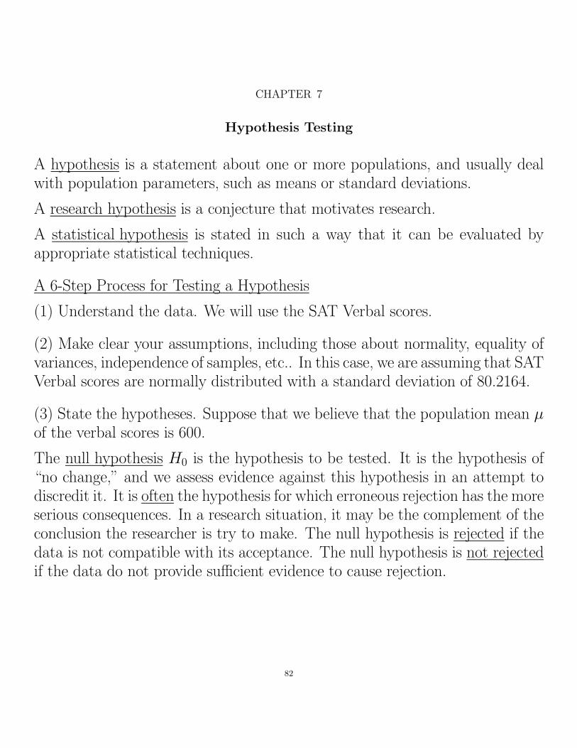
(5) Make a statistical decision. The typical a priori levels of significance are↵ = .05 and ↵ = .01. These are the most commonly used significance levels inpublished research. Since our alternative hypothesis is two-sided because it con-tains 6=, these significance levels are divided equally on both sides of the mean.The diagram on the next page shows the case for ↵ = .05, with probability↵
2=
.05
2= .025 in each tail. We show the acceptance and rejection regions
below using both the x scores and the standardized z scores. The ↵ = .05acceptance region for the x scores is just the 95% confidence interval aboutthe hypothesized mean µ = 600. Press APPS>1:FlashApps>Stats/ListEditor>F7:Ints>1:ZInterval and choose Stats as Data Input Method.Then press ENTER.Fill in the table with our information and press ENTER.Weget the interval (554.6, 645.4) as shown in the following diagram.
7. HYPOTHESIS TESTING 85
Since our test statistics of x = 550.83 and z = �2.1231 are in the rejectionregion, we reject the null hypothesis of µ = 600. A test statistic that falls inthe rejection region is called significant.
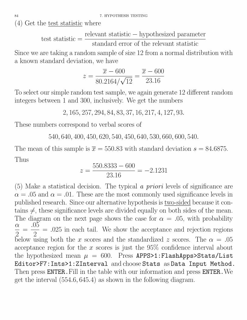
The next case we show is for ↵ = .01, with probability↵
2=
.01
2= .005 in each
tail.
In this case the test statistics of x = 550.83 and z = �2.1231 are in theacceptance region, so there is insu�cient evidence to reject the null hypothesis.
In general, if H0 is rejected, we conclude HA is true, and if H0 is not rejected,we conclude H0 may be true.
(6) Find the p-value, the probability that the test statistic would take a valueas extreme or more extreme than that observed if if H0 were true. The smaller

86 7. HYPOTHESIS TESTING
p is, the more evidence there is against H0. In the past p-values were di�cultto compute. That is why researchers used set significance values like ↵ = .05and ↵ = .01 which did not require them to find p-values. But p-values are nowreadily available to us by calculator and computer.
For our problem, take the TI and enter APPS>1:FlashApps>Stats/ListEditor>F6:Tests>1:ZTest and choose Stats as Data Input Method. Thenpress ENTER.Fill in the table with our information and press ENTER. Put in600 for µ0, 80.2164 for �, 550.83 for x, and 12 for n. Choose µ 6= µ0 forAlternate Hyp, and Draw for Results.
We see that p = .033722. Note that this is smaller than .05 and greater than.01, causing us to reject the null hypothesis at the ↵ = .05 significance levelbut not at the ↵ = .01 significance level.
A more modern approach to hypothesis testing is, instead of using preset sig-nificance levels, to find the p-value and then make decisions based on it.
(30) Suppose we believe that there is no way the population mean could beabove 600 for the SAT Verbal scores. Then we would use a one-sided test.
H0 : µ � 600
H1 : µ < 600
(40) To find the boundaries of the one-sided rejection region for an ↵ = .05 signif-icance level, we note that we want the boundary to be the point where the area
7. HYPOTHESIS TESTING 87
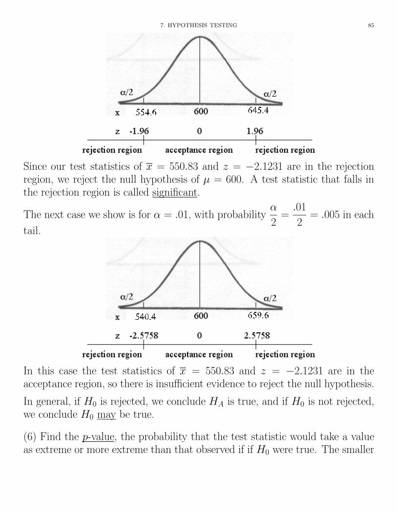
(probability) to the left of it is .05. On the TI for the x-score, assuming we are inthe Data/List Editor, we can find this by F5:Distr>2:Inverse>1:InverseNormal, and in the window that opens put in .05 for Area, 600 for µ, and23.16 for �. Pressing Enter, we get x = 561.9. If we repeat the process andenter 0 for µ and 1 for �, we get z = �1.6449.
(50)
Since our test statistics of x = 550.83 and z = �2.1231 are in the rejectionregion, we reject the null hypothesis of µ = 600.
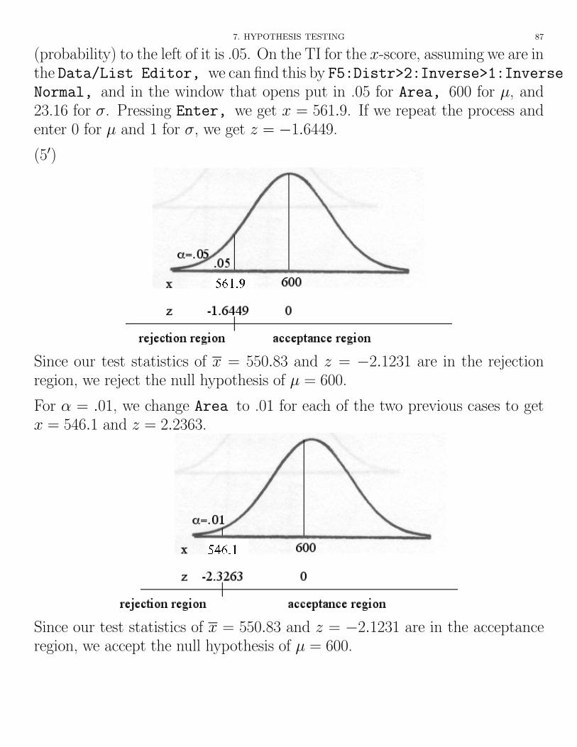
For ↵ = .01, we change Area to .01 for each of the two previous cases to getx = 546.1 and z = 2.2363.
Since our test statistics of x = 550.83 and z = �2.1231 are in the acceptanceregion, we accept the null hypothesis of µ = 600.
88 7. HYPOTHESIS TESTING
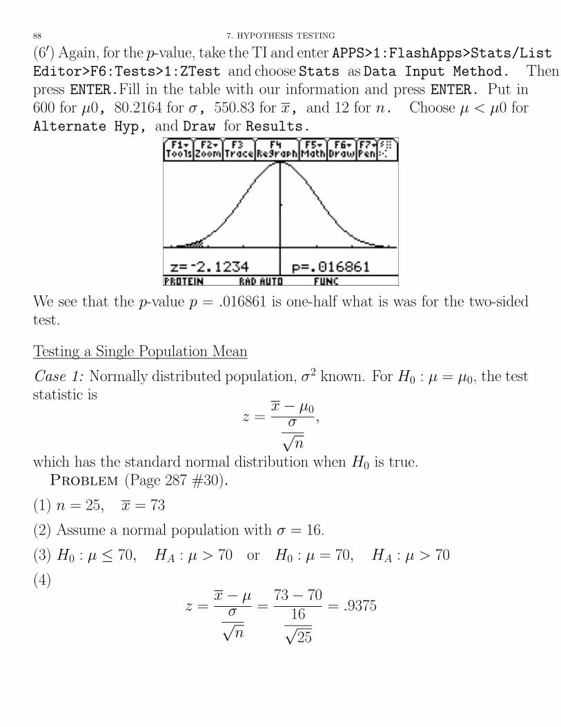
(60) Again, for the p-value, take the TI and enter APPS>1:FlashApps>Stats/ListEditor>F6:Tests>1:ZTest and choose Stats as Data Input Method. Thenpress ENTER.Fill in the table with our information and press ENTER. Put in600 for µ0, 80.2164 for �, 550.83 for x, and 12 for n. Choose µ < µ0 forAlternate Hyp, and Draw for Results.
We see that the p-value p = .016861 is one-half what is was for the two-sidedtest.
Testing a Single Population Mean
Case 1: Normally distributed population, �2 known. For H0 : µ = µ0, the teststatistic is
z =x� µ0
�pn
,
which has the standard normal distribution when H0 is true.Problem (Page 287 #30).
(1) n = 25, x = 73
(2) Assume a normal population with � = 16.
(3) H0 : µ 70, HA : µ > 70 or H0 : µ = 70, HA : µ > 70
(4)
z =x� µ
�pn
=73� 70
16p25
= .9375

7. HYPOTHESIS TESTING 89
(5) Assuming H0 : µ = 70, and since 70 + 1.6449 · 16p25
= 75.2637, a 95% CI
for µ is (�1, 75.2637).
Since x = 73 is in the acceptance range, H0 is not rejected and we continue touse µ = 70 as the population mean.
(6) Since p = .17421 > .05, there is insu�cient evidence to reject H0.
Case 2: Normally distributed population with �2 unknown. The test statistic,for H0 : µ = µ0, is
t =x� µ0
spn
with n� 1 degrees of freedom.
90 7. HYPOTHESIS TESTING
Problem (7.2.12).
(1) n = 15. From TI, x = 13.4267 and s = 1.2820.
(2) We assume a normal population.
(3) H0 : µ = 12 HA : µ 6= 12
(4)
t =13.4267� 12
1.2820p15
= 4.311
The 95% CI for µ, given µ = 12, is 12 ± 2.14479 ⇤ 1.2820p15
= (11.29, 12.71).
11.29 12.71
rejection acceptance rejection
xt -2.1448 2.1448
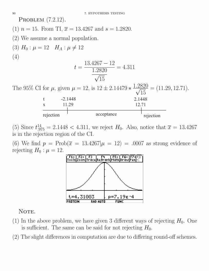
(5) Since t14.975 = 2.1448 < 4.311, we reject H0. Also, notice that x = 13.4267
is in the rejection region of the CI.
(6) We find p = Prob(x = 13.4267|µ = 12) = .0007 as strong evidence ofrejecting H0 : µ = 12.
Note.
(1) In the above problem, we have given 3 di↵erent ways of rejecting H0. Oneis su�cient. The same can be said for not rejecting H0.
(2) The slight di↵erences in computation are due to di↵ering round-o↵ schemes.

7. HYPOTHESIS TESTING 91
Case 3: Sampling from a nonnormal population. For large n, we use theCentral Limit Theorem. For H0 : µ = µ0, the test statistic is
z =x� µ0
�pn
.
One may use s to estimate �.Problem (Page 294 #47).
prex = 392.4394, s = 125.9502, n = 66
postx = 343.2424, s = 105.4316, n = 66
We shall work only with the post numbers at this time. We can assume the sam-pling distribution is not approximately normally distributed, and we estimate� with s. We test
H0 : µ = 392 HA : µ < 392
with ↵ = .01. The 99% CI for µ, given µ = 392 and 392� 2.3263 · 105.4316p66
=
361.8, is (361.8,1).
-2.3263
rejection acceptance
zx 361.8
Clearly, x = 343.2424 is in the rejection region. Also, the test statistic is
z =343.2424� 392
105.4316p66
= �3.7570
is less than �2.3263 and
p = Prob(x = 343.2424|µ = 392) = .000086.
We clearly reject H0.

92 7. HYPOTHESIS TESTING
The Di↵erence between Two Population Means
Case 1: Normally distributed populations with population variances known.We are testing
H0 : µ1 � µ2 = (µ1 � µ2)0 HA : µ1 � µ2 6= (µ1 � µ2)0,
etc., where (µ1 � µ2)0 is the hypothesized di↵erence. If (µ1 � µ2)0 = 0, wecould also use
H0 : µ1 = µ2 HA : µ1 6= µ2.
For H0 : µ1 � µ2 = (µ1 � µ2)0, the test statistic is
z =(x1 � x2)� (µ1 � µ2)0s
�21
n1+
�22
n2
Case 2: Normally distributed populations with population variances unknown,but assumed equal. For H0 : µ1 � µ2 = (µ1 � µ2)0, the test statistic is
tn1+n2�2 =(x1 � x2)� (µ1 � µ2)0s
s2p
n1+
s2p
n2
with pooled variance
s2p =
(n1 � 1)s21 + (n2 � 1)s2
2
n1 + n2 � 2.
7. HYPOTHESIS TESTING 93
Problem (7.3.6). We have the following data:
Sample n x s1 15 4.75 1.02 22 3.00 1.5
We assume the samples come from normally distributed populations with equalvariances. We test
H0 : µ1 � µ2 0 HA : µ1 � µ2 > 0
with ↵ = .05. We find t35.95 = 1.6896. We also have
s2p =
(14)1.02 + (21)1.52
35= 1.75
Assuming H0 : µ1 � µ2 0, and noting
1.6896
r1.75
15+
1.75
22= .7484,
a 95% CI for µ1 � µ2 is (�1, .7484).
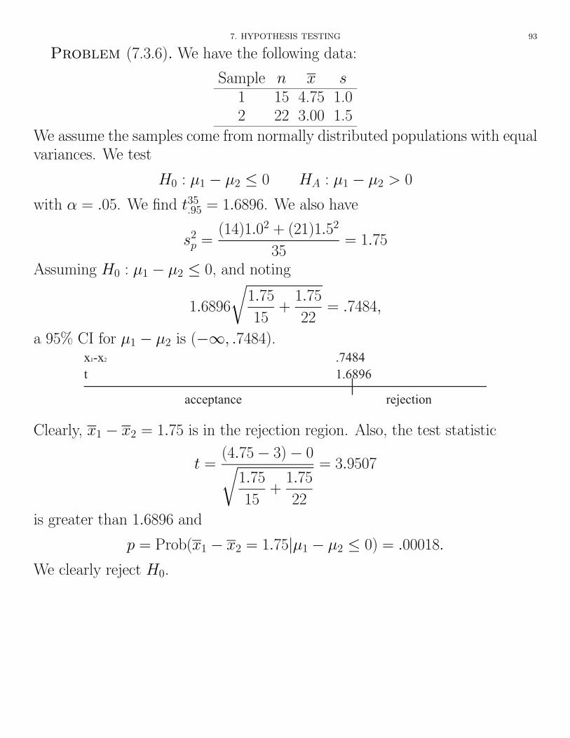
t 1.6896
acceptance rejection
x1-x2 .7484
Clearly, x1 � x2 = 1.75 is in the rejection region. Also, the test statistic
t =(4.75� 3)� 0r
1.75
15+
1.75
22
= 3.9507
is greater than 1.6896 and
p = Prob(x1 � x2 = 1.75|µ1 � µ2 0) = .00018.
We clearly reject H0.
94 7. HYPOTHESIS TESTING
Case 3: Normally distributed population, variances unknown and not knownto be equal. For H0 : µ1 � µ2 = (µ1 � µ2)0, the test statistic is
t⌫ =(x1 � x2)� (µ1 � µ2)0s
s21
n1+
s22
n2
where
⌫ =
s2
1
n1+
s22
n2
�2
" ⇣s21
n1
⌘2
n1 � 1+
⇣s22
n2
⌘2
n2 � 1
#.
Note. We again di↵er from the text here, but align with the TI and SPSS.
Problem (7.3.6). We again have the following data:
Sample n x s1 15 4.75 1.02 22 3.00 1.5
We now assume the samples come from normally distributed populations withunequal variances. We test
H0 : µ1 � µ2 0 HA : µ1 � µ2 > 0
with ↵ = .05. We find
⌫ =
12
15+
1.52
22
�2
"⇣12
15
⌘2
14+
⇣1.52
22
⌘2
21
# = 35
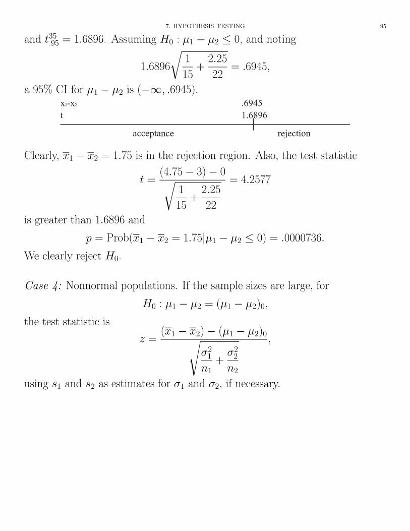
7. HYPOTHESIS TESTING 95
and t35.95 = 1.6896. Assuming H0 : µ1 � µ2 0, and noting
1.6896
r1
15+
2.25
22= .6945,
a 95% CI for µ1 � µ2 is (�1, .6945).
t 1.6896
acceptance rejection
x1-x2 .6945
Clearly, x1 � x2 = 1.75 is in the rejection region. Also, the test statistic
t =(4.75� 3)� 0r
1
15+
2.25
22
= 4.2577
is greater than 1.6896 and
p = Prob(x1 � x2 = 1.75|µ1 � µ2 0) = .0000736.
We clearly reject H0.
Case 4: Nonnormal populations. If the sample sizes are large, for
H0 : µ1 � µ2 = (µ1 � µ2)0,
the test statistic is
z =(x1 � x2)� (µ1 � µ2)0s
�21
n1+
�22
n2
,
using s1 and s2 as estimates for �1 and �2, if necessary.

96 7. HYPOTHESIS TESTING
Problem (Page 284 #20). We have the following data:
Treatment n x sx
(1) Etanercept 40 5.56 0.84(2) Etanercept+methotrexate 57 4.40 0.57
We assume the samples come from nonnormally distributed populations. Since
sx =spn
, s = sxp
n. Thus s1 = .84p
40 and s2 = .57p
57. For
H0 : µ1 � µ2 = 0
with ↵ = .05, the test statistic is
z =(5.56� 4.40)� 0s
(.84p
40)2
40+
(.57p
57)2
57
= 1.1427.
Assuming H0 : µ1 � µ2 = 0 a 95% CI for µ1 � µ2 is
0 ± 1.96
s(.84
p40)2
40+
(.57p
57)2
57= (�1.9897, 1.9897).
-1.9897 1.9897
rejection acceptance rejection
xz -1.96 1.96
x1 � x2 = 1.16 is in the acceptance region, as is the test statistic z = 1.1427.Also,
p = Prob(x1 � x2 = 1.16|µ1 � µ2 = 0) = .253161 > .05.
We do not reject H0 and continue to treat the population means as equal.

7. HYPOTHESIS TESTING 97
Paired Comparisons – the samples are not independent here. The idea is toremove extraneous factors, keeping as many variables as possible the same.Examples are before and after, left and right, identical twins, etc.
But:
(1) It takes time and money to create matches.
(2) You are left with only n� 1 df instead of 2n� 2.
We compute di↵erences d, so this is really a one-sample test. For
H0 : µd = µd0,
the test statistic is
tn�1 =d� µd0
sd
,
where d is the sample mean di↵erence, µd0 is the hypothesized mean di↵erence,
and sd =sdpn.
Problem (Page 294 #47).
We assume a normally distributed population of di↵erences. We can assumethe sampling distribution is approximately normally distributed. We have
d = �49.197, sd = 92.197, n = 66, sd = 11.349
We testH0 : µd � 0 HA : µd < 0
with ↵ = .05. The 95% CI for µd, given µd = 0 and 0 � 1.6686(11.349) =�18.9369, is (�18.9369,1).
-1.6686
rejection acceptance
td -18.9369
Clearly, d = �49.197 is in the rejection region. Also, the test statistic
t =�49.197� 0
11.349= �4.3351

98 7. HYPOTHESIS TESTING
is less than �1.6686 and
p = Prob(d = �49.197|µd � 0) = .0000259.
We clearly reject H0.
A Single Population Proportion
ForH0 : p = p0 HA : p 6= p0,
ifnp0 � 5, and n(1� p0) � 5
so that the Central Limit Theorem applies, use
z =bp� p0rp0(1� p0)
nas the test statistic.
Note. We use p0 rather than bp in the formula since p0 is hypothesized asthe true population proportion.
7. HYPOTHESIS TESTING 99
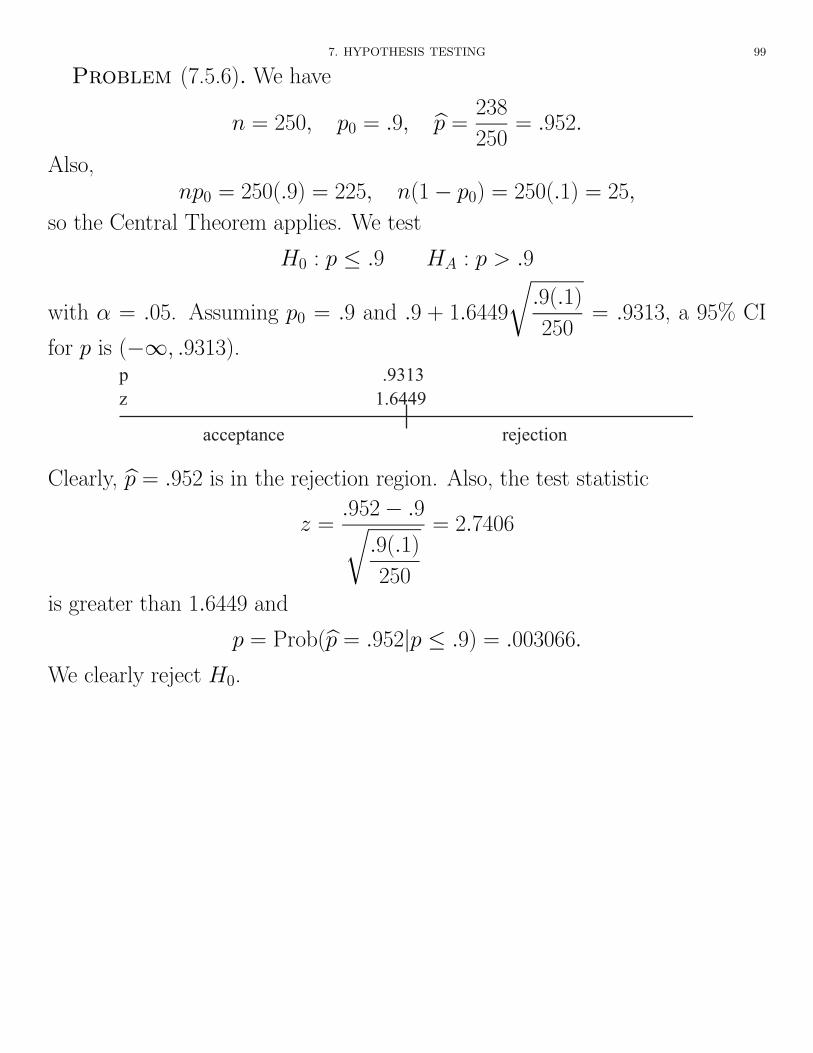
Problem (7.5.6). We have
n = 250, p0 = .9, bp =238
250= .952.
Also,np0 = 250(.9) = 225, n(1� p0) = 250(.1) = 25,
so the Central Theorem applies. We test
H0 : p .9 HA : p > .9
with ↵ = .05. Assuming p0 = .9 and .9 + 1.6449
r.9(.1)
250= .9313, a 95% CI
for p is (�1, .9313).
1.6449
acceptance rejection
zp .9313
Clearly, bp = .952 is in the rejection region. Also, the test statistic
z =.952� .9r
.9(.1)
250
= 2.7406
is greater than 1.6449 and
p = Prob(bp = .952|p .9) = .003066.
We clearly reject H0.
100 7. HYPOTHESIS TESTING
The Di↵erence between Two Population Proportions
For
H0 : p1 � p2 = (p1 � p2)0,
based on the hypothesis that (p1 � p2)0 = 0, we pool the samples to compute
p =x1 + x2
n1 + n2and b�bp1�bp2 =
sp(1� p)
n1+
p(1� p)
n2.
Our test statistic is then
z =(bp1 � bp2)� (p1 � p2)0
b�bp1�bp2
,
which is approximately normally distributed if H0 is true.
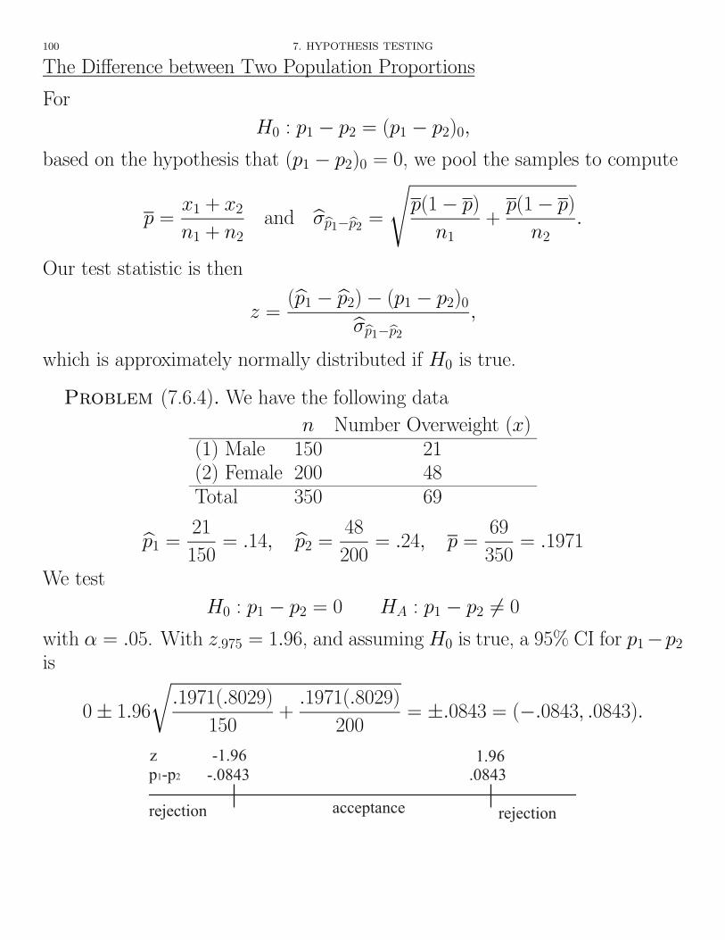
Problem (7.6.4). We have the following data
n Number Overweight (x)(1) Male 150 21(2) Female 200 48Total 350 69
bp1 =21
150= .14, bp2 =
48
200= .24, p =
69
350= .1971
We test
H0 : p1 � p2 = 0 HA : p1 � p2 6= 0
with ↵ = .05. With z.975 = 1.96, and assuming H0 is true, a 95% CI for p1�p2
is
0 ± 1.96
r.1971(.8029)
150+
.1971(.8029)
200= ±.0843 = (�.0843, .0843).
-.0843 .0843
rejection acceptance rejection
p1-p2z -1.96 1.96

7. HYPOTHESIS TESTING 101
Our test statistic is
z =(.14� .24)� 0r
.1971(.8029)
150+
.1971(.8029)
200
=�.1
.043= �2.3256,
which lies in the rejection region as does bp1 � bp2 = �.1. We also have p =.0200 < .05
The Type II Error and the Power of a Test
accept H0 reject H0
H0 true correct decision Type I error (↵)H0 false Type II error (�) correct decision
Type II Error – failing to reject H0 when H0 is false.
We set ↵, the probability of a Type I error.
Power of a Test = 1� � = Prob(rejecting H0|H0 is false).
� depends on
(1) The true value of the parameter of interest.
(2) The hypothesized value of the parameter.
(3) ↵
(4) n
� and 1 � � may be computed for any alternative value of the parameter weare testing.
Example (7.9.1). A two-sided example.
� = 3.6, n = 100, ↵ = .05
H0 : µ = 17.5 HA : µ 6= 17.5

102 7. HYPOTHESIS TESTING
Upper and lower critical x-values:
xU = µ0 + z�pn
= 17.5 + 1.96⇣3.6
10
⌘= 18.21
xL = µ0 � z�pn
= 17.5� 1.96⇣3.6
10
⌘= 16.79
Suppose H0 is false with true mean = µ1 = 16.5. This gives the normalsampling distribution f(x1). The hypothesized mean gives the sampling distri-bution f(x0).
� = the area under the curve of f(x1) that overlaps the nonrejection region off(x0).

7. HYPOTHESIS TESTING 103
� = P (16.79 x 18.21|µ = 16.5,� = .36) =
nmcdf(16.79, 18.21, 16.5, .36) = .2102.
Power of the test = 1� � = .7898.Note.
(1) The further µ1 is from µ0, the smaller � is.
(2) To make � smaller, increase n.
Example (7.9.2). A one-sided example.
� = 15, n = 20, ↵ = .01
H0 : µ � 65 H1 : µ < 65
xL = 65� 2.3263⇣ 15p
20
⌘= 57.1974
Suppose H0 is false with a true mean of µ1 = 55.
� = P⇣x > 57.1974|µ = 55,� =
15p2
⌘=
nmcdf(57.1974, 1E99, 55,15p
2) = .2562.
Power of the test = 1� � = .7438
Note. The text’s numbers di↵er from ours due to excessive rounding.