Hypothesis testing for the GLM

The General Linear Hypothesis

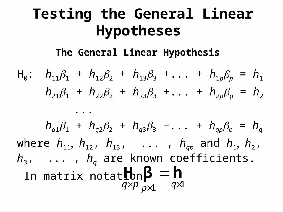
Testing the General Linear Hypotheses

The General Linear Hypothesis H0: h111 + h122 + h133 +... + h1pp = h1

h211 + h222 + h233 +... + h2pp = h2

...

hq11 + hq22 + hq33 +... + hqpp = hq

where h11h12, h13, ... , hqp and h1h2, h3, ... , hq are known coefficients.

In matrix notation11

qppqhβH

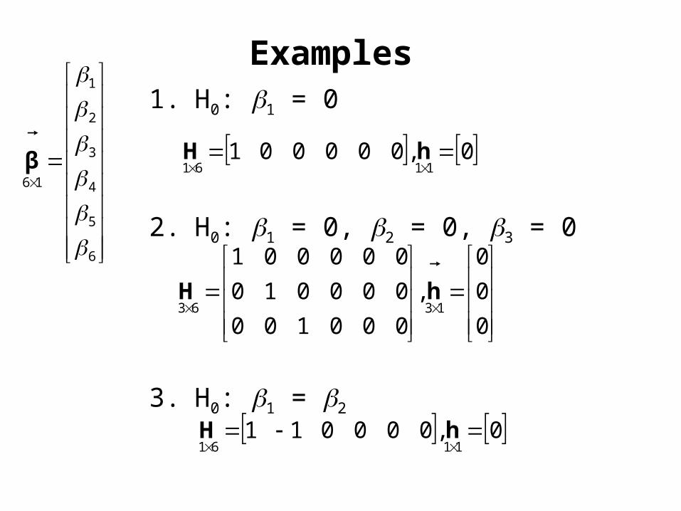
Examples 1. H0: 1 = 0

2. H0: 1 = 0, 2 = 0, 3 = 0

3. H0: 1 = 2

6

5

4

3

2

1

16

β 0,000001

1161

hH

0

0

0

,

000100

000010

000001

1363hH

0,0000111161

hH

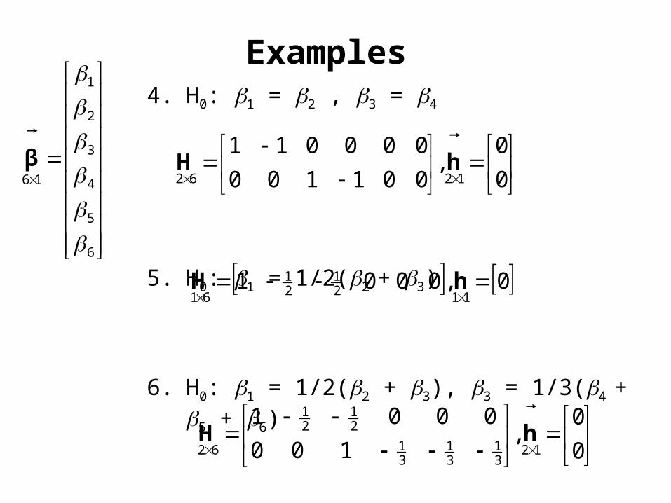
Examples 4. H0: 1 = 2 , 3 = 4

5. H0: 1 = 1/2(2 + 3)

6. H0: 1 = 1/2(2 + 3), 3 = 1/3(4 + 5 + 6)

6

5

4

3

2

1

16

β

0

0,

001100

0000111262

hH

0,0001112

121

61

hH

0

0,

100

000112

31

31

31

21

21

62hH

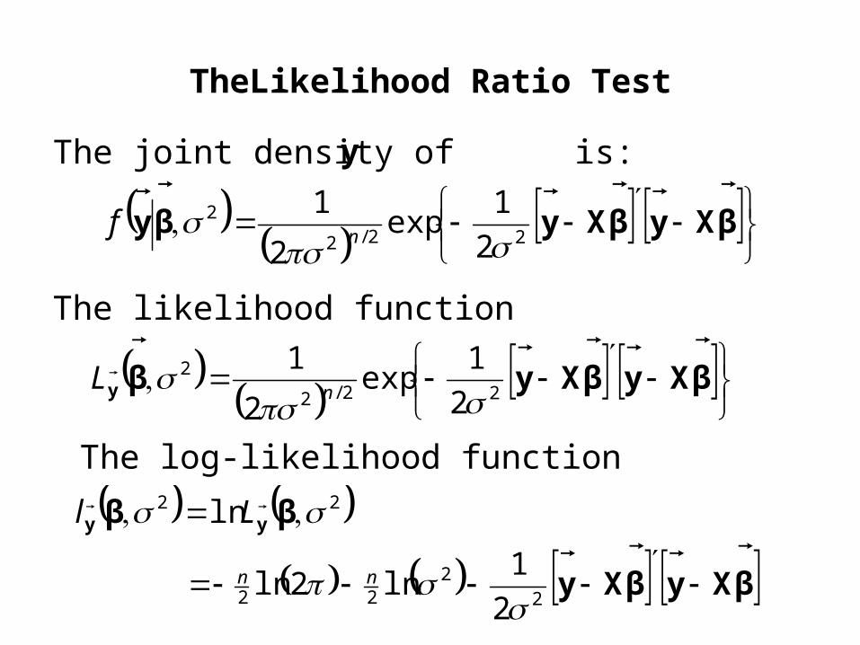
TheLikelihood Ratio Test

The joint density of is:

βXyβXyβy

22/2

2

2

1exp

2

1

nf

y

The likelihood function

βXyβXyβy

22/2

2

2

1exp

2

1

nL

The log-likelihood function

βXyβXy

ββ yy

22

22

22

2

1ln2ln

ln

nn

Ll

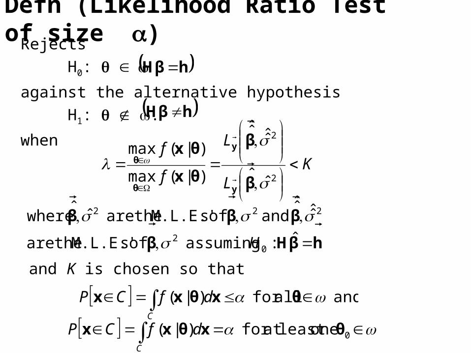
Defn (Likelihood Ratio Test of size )Rejects

H0:

against the alternative hypothesis

H1: .

when

and K is chosen so that

KL

L

f

f

2

2

ˆˆ

ˆ̂ˆ̂

)|(max

)|(max

β

β

θx

θx

y

y

θ

θ

and allfor )|( θxθxxC

dfCP

0 oneleast at for )|( θxθxxC

dfCP

hβH

hβH

hβHβ

βββ

ˆ: assuming of sM.L.E.' theare

ˆ̂ˆ̂ and of sM.L.E.' theare ˆˆ where

02

222

H

Note

2ˆ̂ and ˆ̂

find To β

We will maximize.

condition side thesubject to ly equivalent

2

1ln2ln

2

22

222

β

βXyβXyβ

y

y

L

l nn

βXyβXyyXXXβ ˆˆˆ and ˆ 121

n

hβH

:0H

The Lagrange multiplier technique will be used for this purpose

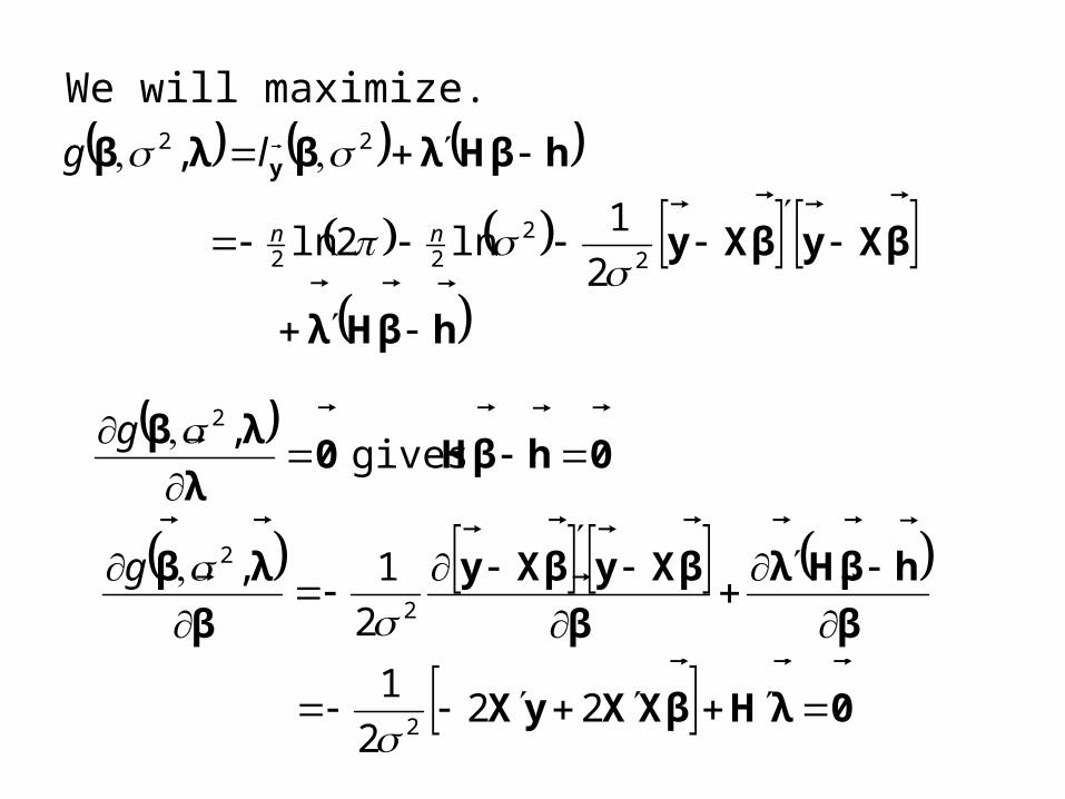
We will maximize.

hβHλ

βXyβXy

hβHλβλβ y

2

1ln2ln

,

22

22

22

nn

lg

0hβH0

λ

λβ

gives ,2g

β

hβHλ

β

βXyβXy

β

λβ

2

2

2

1,

g

0λHβXXyX

222

12

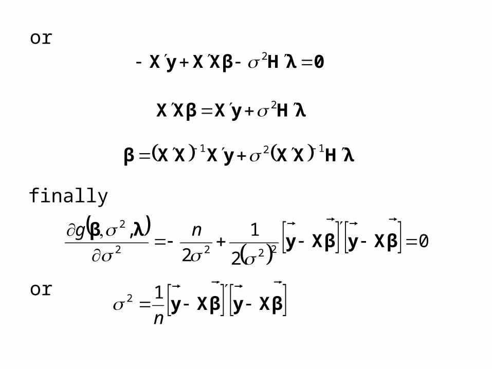
or0λHβXXyX

2

λHyXβXX 2

λHXXyXXXβ 121

0

2

1

2

,2222

2

βXyβXyλβ

ng

finally

or βXyβXy

n

12

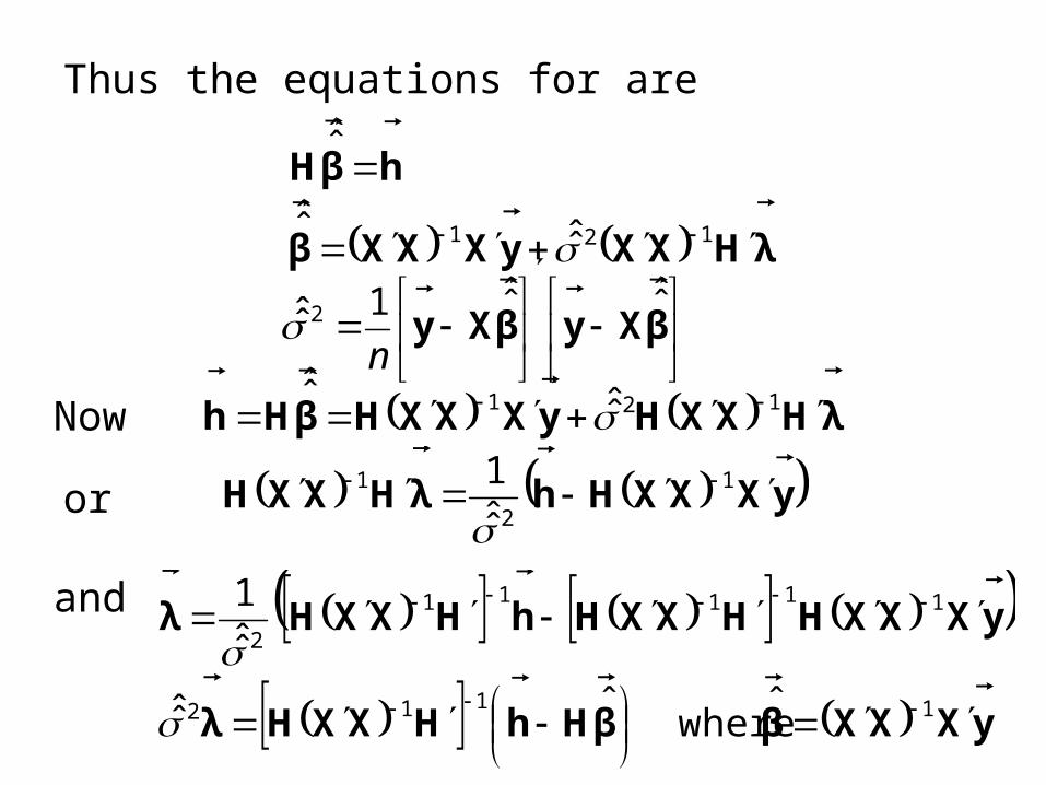
Thus the equations for are

λHXXyXXXβ 121 ˆ̂ˆ̂

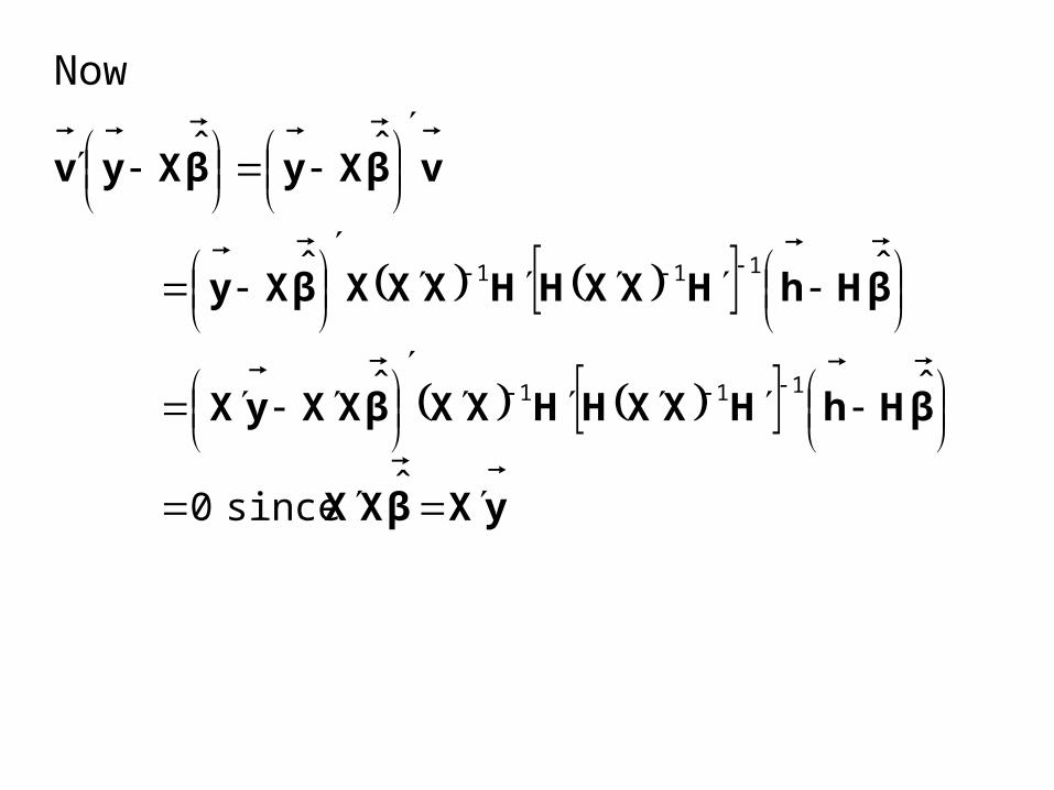
Now

or

βXyβXy

ˆ̂ˆ̂1ˆ̂ 2

n

hβH

ˆ̂

λHXXHyXXXHβHh 121 ˆ̂ˆ̂

yXXXHhλHXXH 1

2

1

ˆ̂1

and yXXXββHhHXXHλ

yXXXHHXXHhHXXHλ

1112

11111

2

ˆ whereˆˆ̂

ˆ̂1

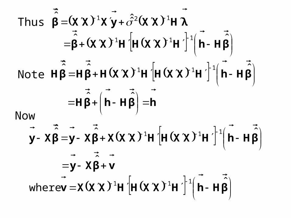
Thus

Now

βHhHXXHHXXβ

λHXXyXXXβ

ˆˆ

ˆ̂ˆ̂

111

121

Note hβHhβH

βHhHXXHHXXHβHβH

ˆˆ

ˆˆˆ̂ 111

βHhHXXHHXXXv

vβXy

βHhHXXHHXXXβXyβXy

ˆ where

ˆ

ˆˆˆ̂

111

111

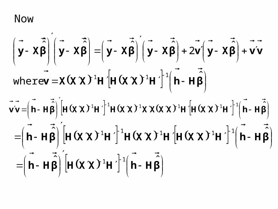
Now

βHhHXXHHXXXv

vvβXyvβXyβXyβXyβXy

ˆ where

ˆ2ˆˆˆ̂ˆ̂

111

βHhHXXHHXXXXXXHHXXHβHhvv ˆˆ 111111

βHhHXXHHXXHHXXHβHh ˆˆ 11111

βHhHXXHβHh ˆˆ 11

Now

yXβXX

βHhHXXHHXXβXXyX

βHhHXXHHXXXβXy

vβXyβXyv

ˆ since 0

ˆˆ

ˆˆ

ˆˆ

111

111

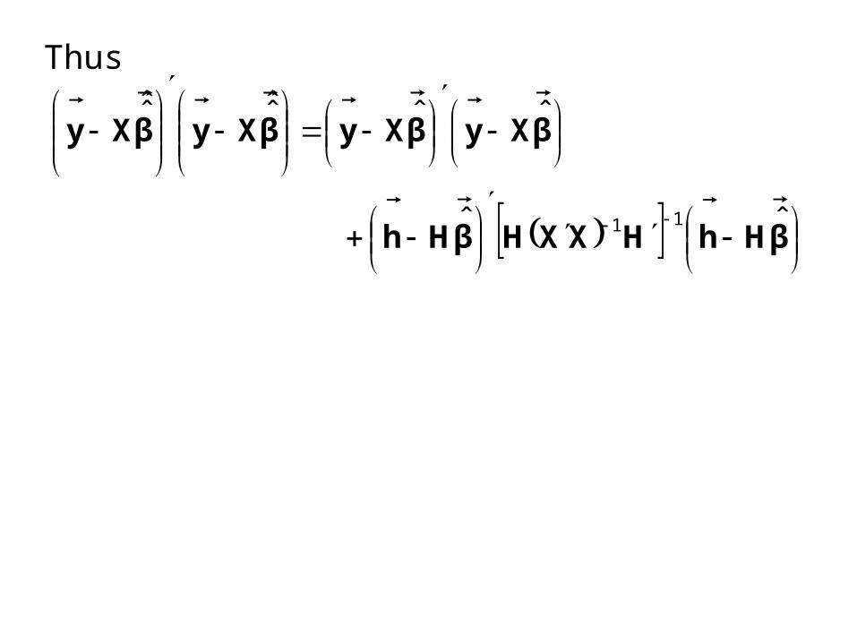
Thus

βHhHXXHβHh

βXyβXyβXyβXy

ˆˆ

ˆˆˆ̂ˆ̂

11

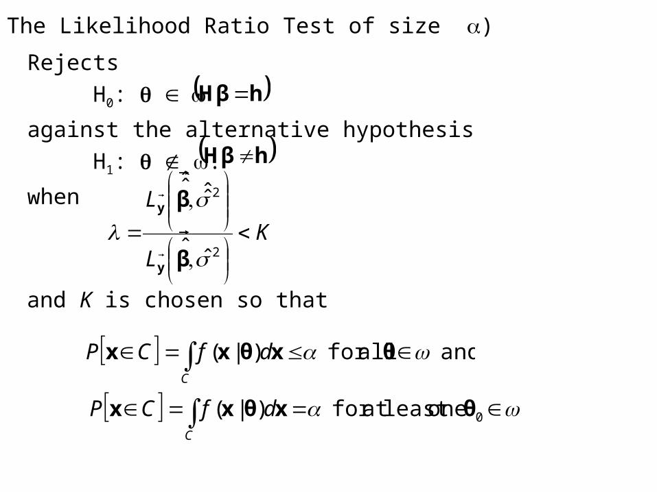
The Likelihood Ratio Test of size )

Rejects

H0:

against the alternative hypothesis

H1: .

when

and K is chosen so that

KL

L

2

2

ˆˆ

ˆ̂ˆ̂

β

β

y

y

and allfor )|( θxθxxC

dfCP

0 oneleast at for )|( θxθxxC

dfCP

hβH

hβH

βXyβXyβy

22/2

2

2

1exp

2

1

nL

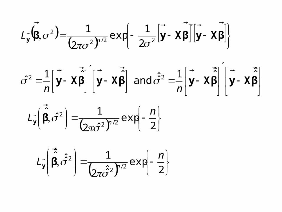
βXyβXyβXyβXy

ˆ̂ˆ̂1ˆ̂ and ˆˆ1ˆ 22

nn

2exp

ˆ2

1ˆˆ

2/2

2 nL n

βy

2exp

ˆ̂2

1ˆ̂ˆ̂2/

2

2 nL n

βy

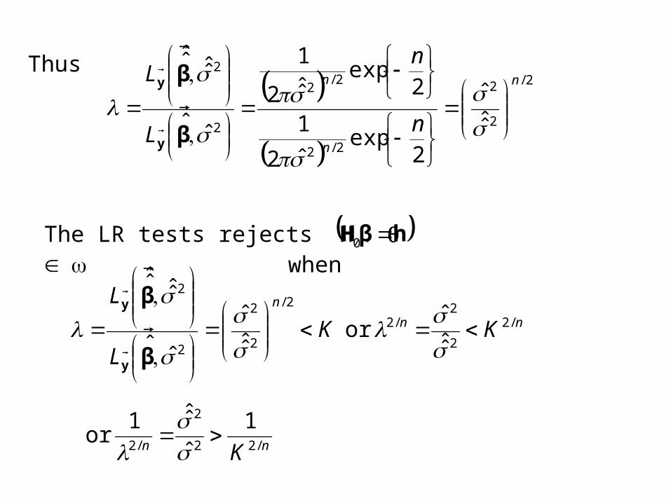
Thus

2/

2

2

2/2

2/2

2

2

ˆ̂ˆ

2exp

ˆ2

1

2exp

ˆ̂2

1

ˆˆ

ˆ̂ˆ̂n

n

n

n

n

L

L

β

β

y

y

The LR tests rejects H0: when

nn

n

KKL

L/2

2

2/2

2/

2

2

2

2

ˆ̂ˆ

or ˆ̂ˆ

ˆˆ

ˆ̂ˆ̂

β

β

y

y

hβH

nn K /22

2

/2

1ˆ

ˆ̂1or

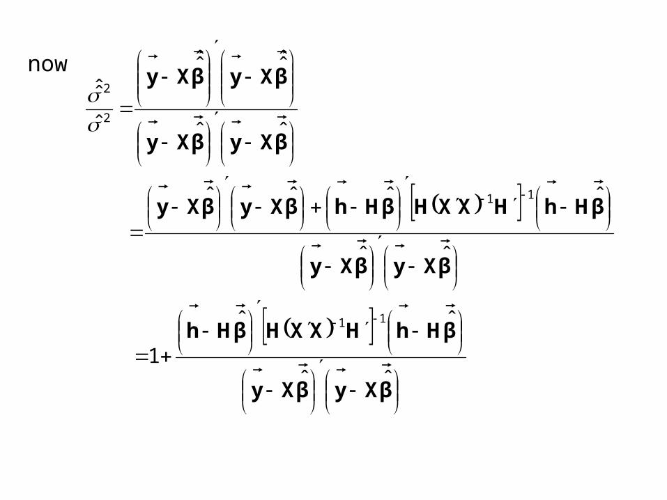
now

βXyβXy

βHhHXXHβHh

βXyβXy

βHhHXXHβHhβXyβXy

βXyβXy

βXyβXy

ˆˆ

ˆˆ

1

ˆˆ

ˆˆˆˆ

ˆˆ

ˆ̂ˆ̂

ˆ

ˆ̂

11

11

2

2

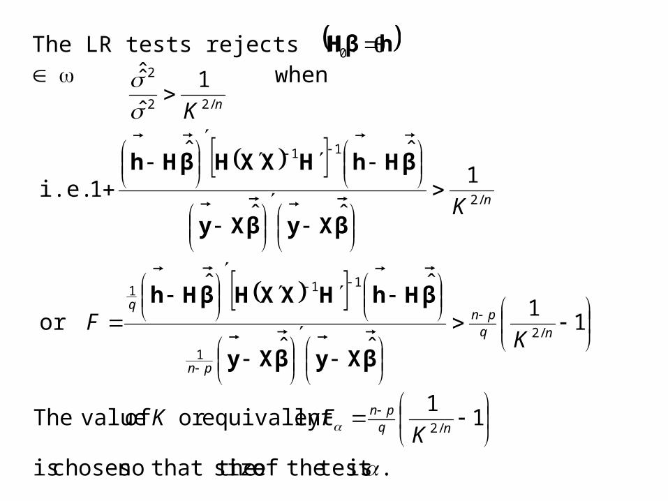
The LR tests rejects H0: when

hβH

11

ˆˆ

ˆˆ

or

1

ˆˆ

ˆˆ

1 i.e.

1ˆ

ˆ̂

/2

1

111

/2

11

/22

2

nqpn

pn

q

n

n

KF

K

K

βXyβXy

βHhHXXHβHh

βXyβXy

βHhHXXHβHh

. is test theof size that thesochosen is

11

ly equivalentor of valueThe/2

nqpn

KFK

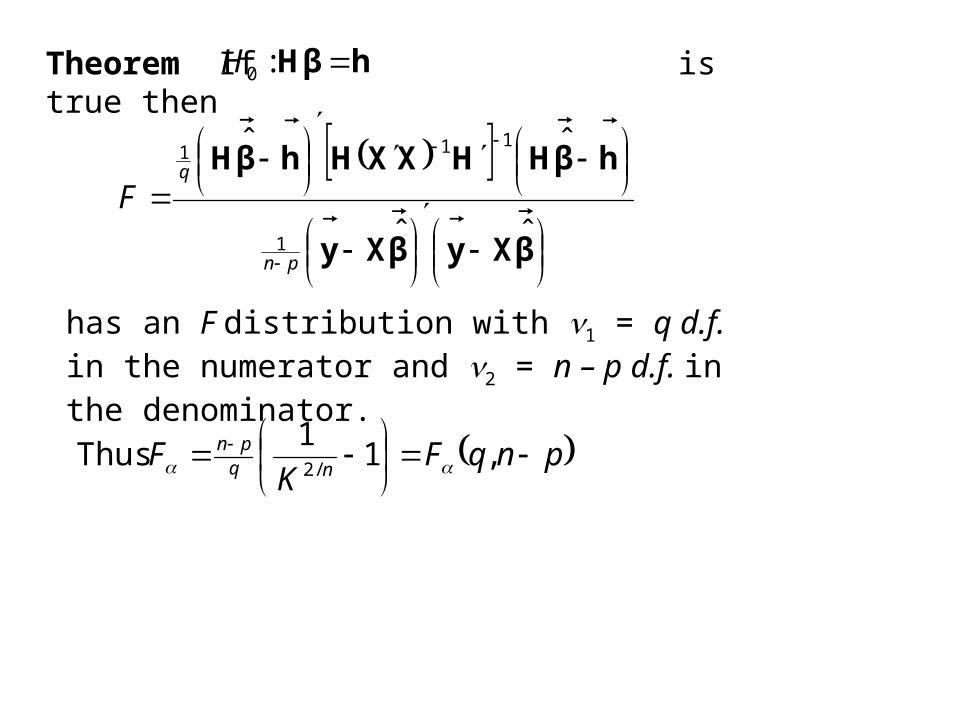
Theorem If is true thenhβH

:0H

βXyβXy

hβHHXXHhβH

ˆˆ

ˆˆ

1

111

pn

q

F

pnqFK

Fnq

pn

,1

1 Thus

/2

has an F distribution with 1 = q d.f. in the numerator and 2 = n – p d.f. in the denominator.

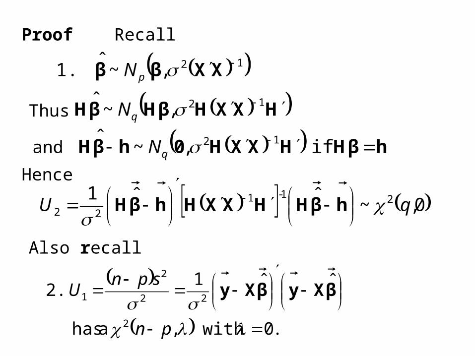
Proof Recall

.0 with , a has

ˆˆ1 2.

2

22

2

1

pn

spnU βXyβXy

12, ~ ˆ 1. XXββ

pN

Thus HXXHβHβH 12, ~ ˆ

qN

and hβHHXXH0hβH

if , ~ ˆ 12qN

Hence

0, ~ ˆˆ1 21-1

22 qU

hβHHXXHhβH

Also recall

βXyβXy ˆˆ1

22

2

1

spnU

Thus

hβHHXXHhβH

ˆˆ1

1-1

22 U

is independent of

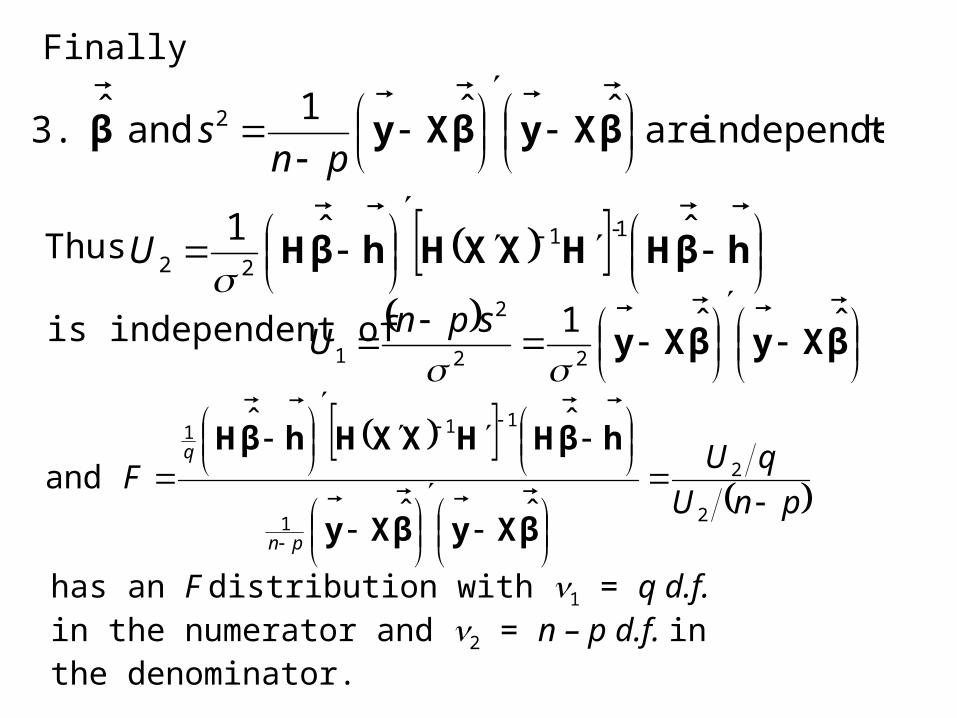
tindependen are ˆˆ1 and ˆ 3. 2

βXyβXyβ

pns

pnU

qUF

pn

q

2

2

1

111

ˆˆ

ˆˆ

and

βXyβXy

hβHHXXHhβH

has an F distribution with 1 = q d.f. in the numerator and 2 = n – p d.f. in the denominator.

Finally

hβHHXXHhβHβXyβXy

ˆˆˆˆ 1-1

0 assuming S.S. residual ˆ̂ˆ̂

0HRSSH

βXyβXy

RSSRSSH

0

ˆˆ 11 hβHHXXHhβH

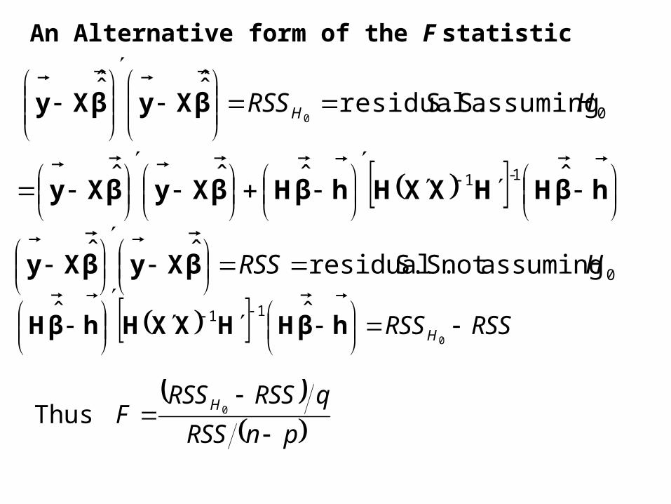
An Alternative form of the F statistic

0 assumingnot S.S. residual ˆˆ HRSS

βXyβXy

pnRSS

qRSSRSSF H

0 Thus

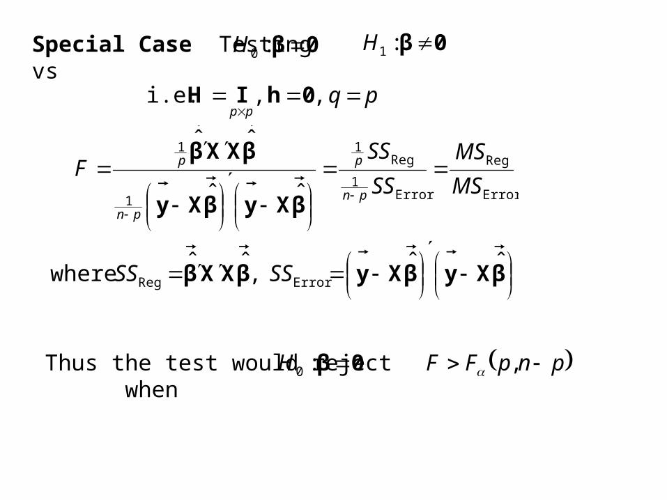
Special Case Testing vs0β

:0H

Error

Reg

Error1

Reg1

1

1

ˆˆ

ˆˆ

MS

MS

SS

SSF

pn

p

pn

p

βXyβXy

βXXβ

0β

:1H

pnpFF ,Thus the test would reject when0β

:0H

pqpp

, , i.e. 0hIH

βXyβXyβXXβ ˆˆ ,ˆˆ where ErrorReg

SSSS

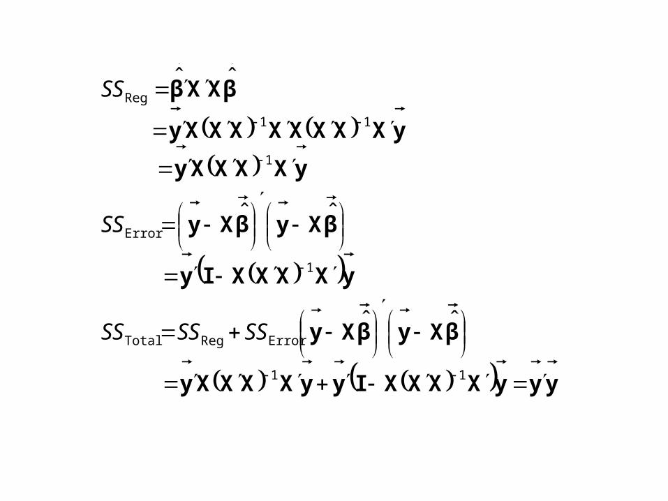
yyyXXXXIyyXXXXy

βXyβXy

yXXXXIy

βXyβXy

yXXXXy

yXXXXXXXXy

βXXβ

11

ErrorRegTotal

1

Error

1

11

Reg

ˆˆ

ˆˆ

ˆˆ

SSSSSS

SS

SS

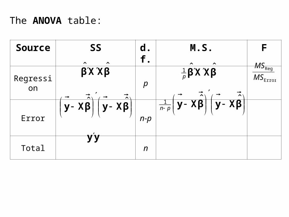
The ANOVA table:

Source SS d.f. M.S. F

Regression p

Error n-p

Total n

βXXβ ˆˆ

βXyβXy ˆˆ1

pn

βXXβ ˆˆ1

p

βXyβXy ˆˆ

yy

Error

Reg

MS

MS

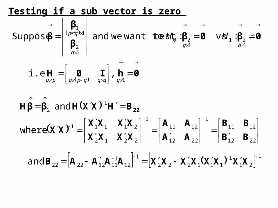
Testing if a sub vector is zero

0β0ββ

ββ

121

120

12

11

: vs: test want to weand Supposeqq

q

qp HH

0hI0H

1 , i.e.

qqqqpqpq

2212

1211

1

2212

1211

1

2212

21111

12

where

and ˆˆ

BB

BB

AA

AA

XXXX

XXXXXX

BHXXHββH 22

1

211

111222

1

121

11122222 and XXXXXXXXAAAAB

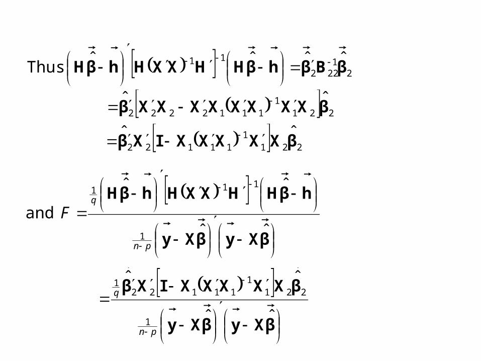
21

222

11 ˆˆˆˆ Thus βBβhβHHXXHhβH

2211

1112222ˆˆ βXXXXXXXXβ

2211

11122ˆˆ βXXXXXIXβ

βXyβXy

hβHHXXHhβH

ˆˆ

ˆˆ

and1

111

pn

q

F

βXyβXy

βXXXXXIXβ

ˆˆ

ˆˆ

1

2211

111221

pn

q

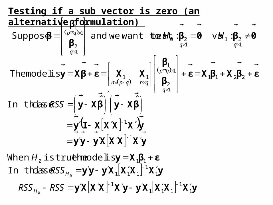
Testing if a sub vector is zero (an alternative formulation)

0β0ββ

ββ

121

120

12

11

: vs: test want to weand Supposeqq

q

qp HH

εβXβXεβ

βXXεβXy

is model The 2211

12

11

11

q

qp

qnqpn

εβXy

110 is model the trueis When H

yXXXXyyy

yXXXXIy

βXyβXy

1

1

ˆˆ case In this RSS

yXXXXyyy

11

111 case In this0

HRSS

yXXXXyyXXXXy

11

1111

0 RSSRSSH

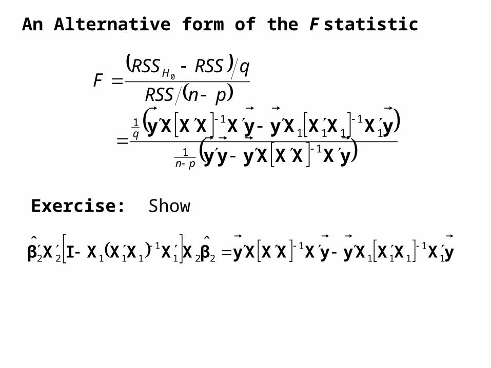
An Alternative form of the F statistic

yXXXXyyy

yXXXXyyXXXXy

11

11

11111

0

pn

q

H

pnRSS

qRSSRSSF

Exercise: Show

yXXXXyyXXXXyβXXXXXIXβ

11

1111

2211

11122ˆˆ

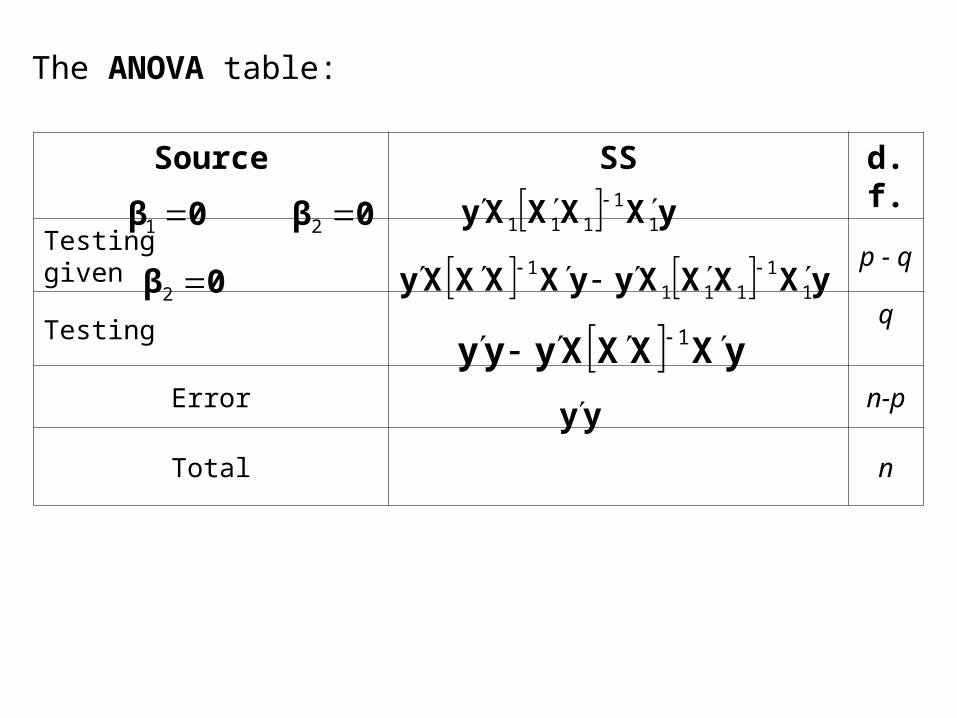
The ANOVA table:

Source SS d.f.

Testing given p - q

Testingq

Error n-p

Total nyy

0β

1 0β

2

0β

2

yXXXXy

11

111

yXXXXyyXXXXy

11

1111

yXXXXyyy 1

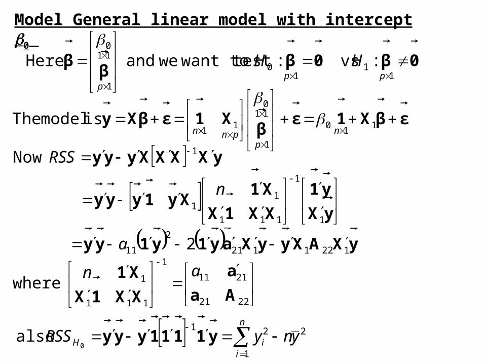
Model General linear model with intercept 0

0β0ββ

β

11

10

1

110

: vs: test want to weand Herepp

p

HH

εβX1εβ

X1εβXy

is model The 1

10

1

110

11 n

ppnn

yX

y1

XX1X

X1Xy1yyy

yXXXXyyy

1

1

111

11

1

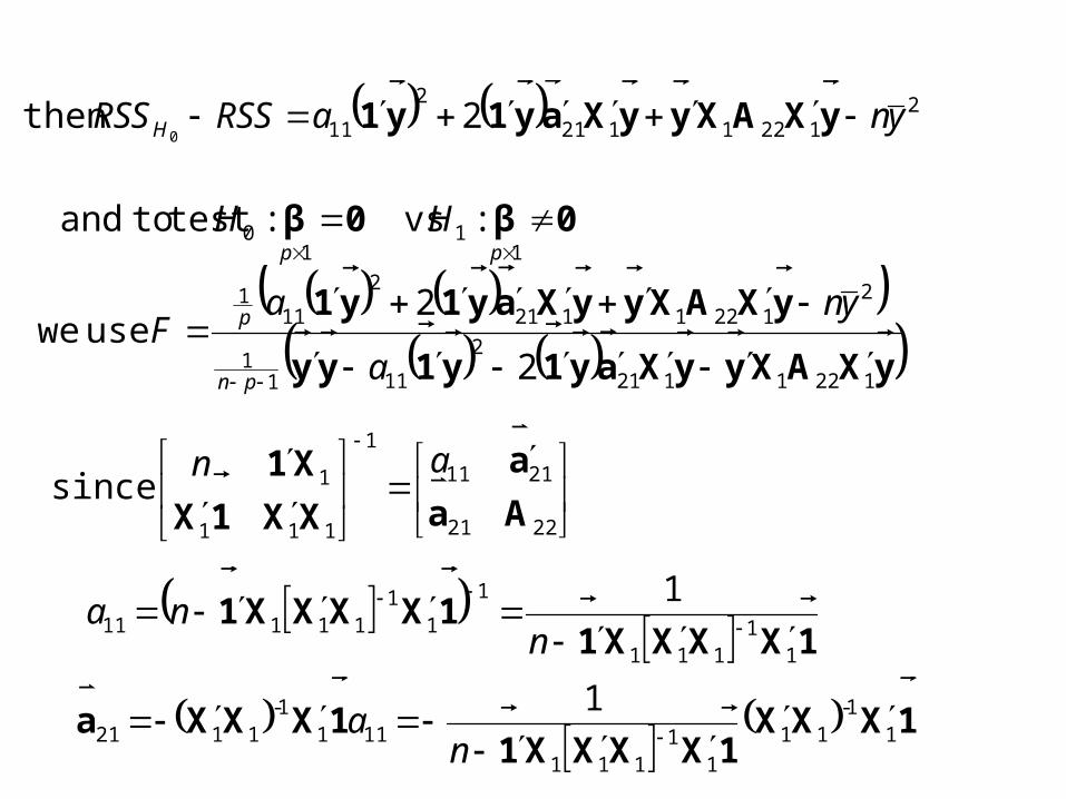
Now

n

RSS

yXAXyyXay1y1yy

1221121

2

11 2 a

2221

2111

1

111

1 whereAa

a

XX1X

X1 an

n

iiH ynyRSS

1

221 also

0y1111yyy

0β0β

1

11

0 : vs: test toandpp

HH

21221121

2

11 2then 0

ynaRSSRSSH yXAXyyXay1y1

yXAXyyXay1y1yy

yXAXyyXay1y1

1221121

2

1111

21221121

2

111

2

2 use we

a

ynaF

pn

p

2221

2111

1

111

1 sinceAa

a

XX1X

X1

an

1XXXX1

1XXXX1

11

111

1

11

11111

1

nna

1XXX1XXXX1

1XXXa

11-

11

11

111

1111-

1121

1

na

21221121

2

11 2then 0

ynaRSSRSSH yXAXyyXay1y1

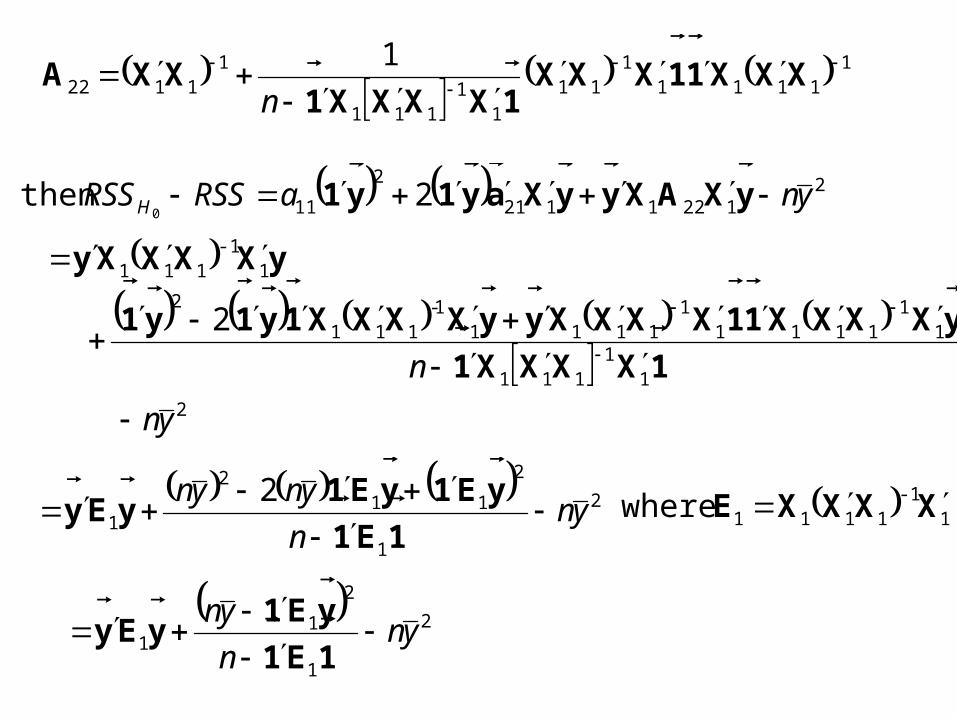
11111

111

11

111

11122

1

XXX11XXX1XXXX1

XXA

n

2

11

111

11

11111

11111-

111

2

1-1

111

2

yn

n

1XXXX1

yXXXX11XXXXyyXXXX1y1y1

yXXXXy

2

1

2

112

1

2yn

n

ynyn

1E1

yE1yE1yEy

1

-11111 where XXXXE

2

1

2

11 yn

n

yn

1E1

yE1yEy

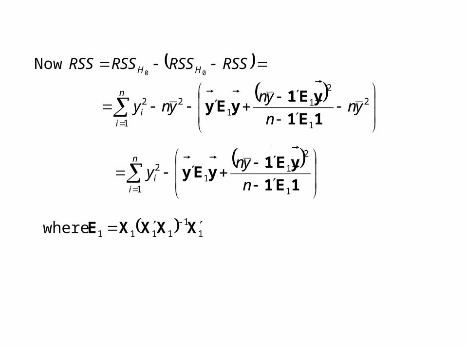
RSSRSSRSSRSS HH 00 Now

2

1

2

11

1

22 ynn

ynyny

n

ii

1E1

yE1yEy

1E1

yE1yEy

1

2

11

1

2

n

yny

n

ii

1-1

1111 where XXXXE

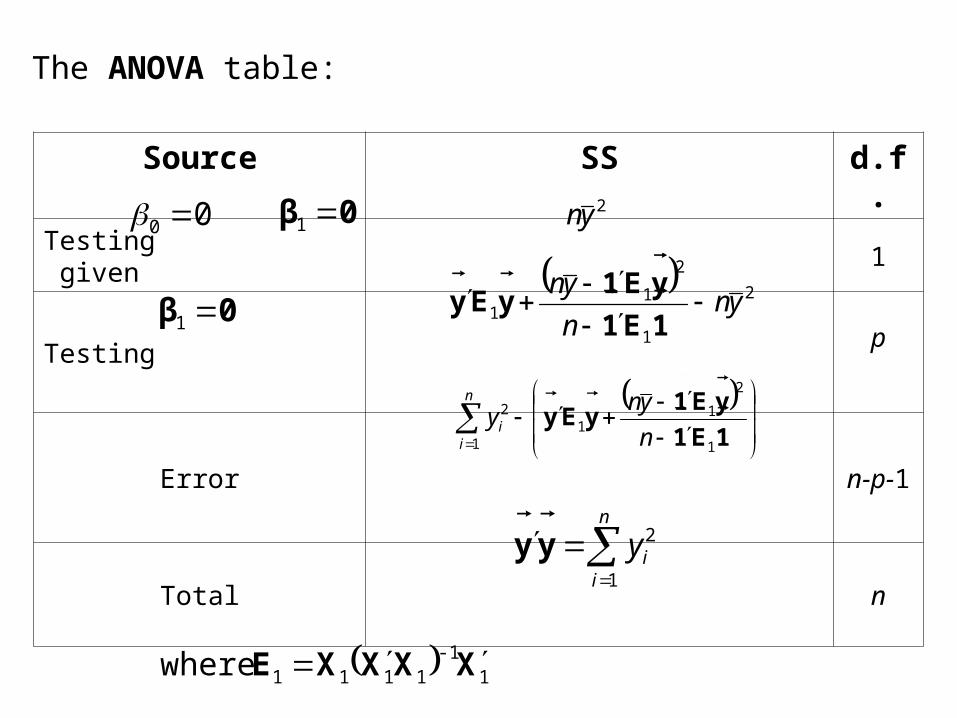
The ANOVA table:

Source SS d.f.

Testing given 1

Testingp

Error n-p-1

Total n

n

iiy

1

2yy

00 0β

1

0β

1

1E1

yE1yEy

1

2

11

1

2

n

yny

n

ii

2

1

2

11 yn

n

yn

1E1

yE1yEy

2yn

1-1

1111 where XXXXE

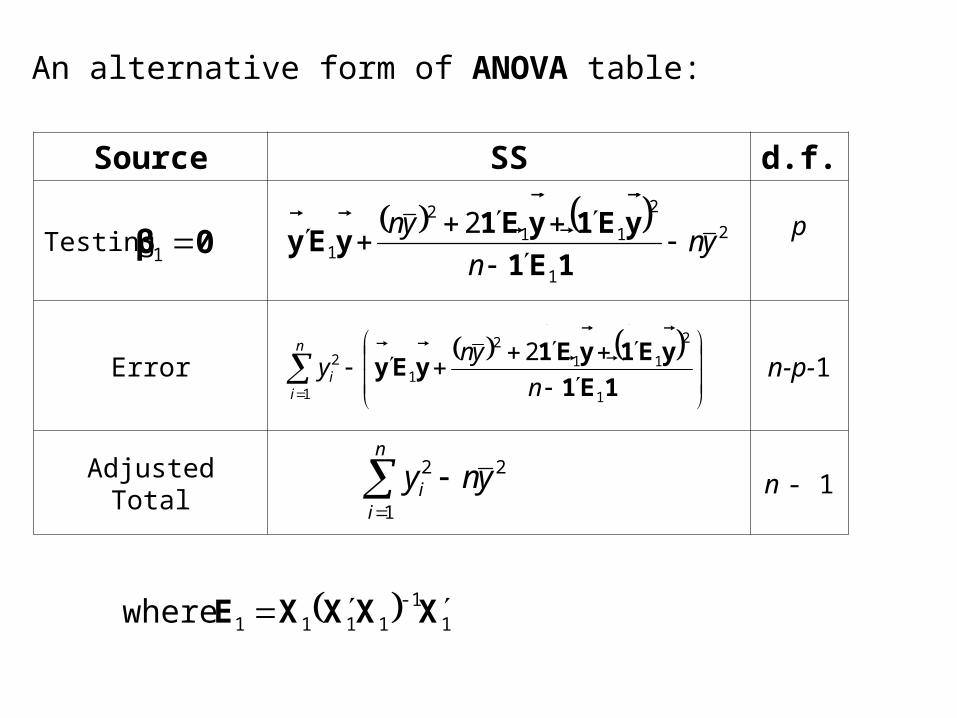
An alternative form of ANOVA table:

Source SS d.f.

Testingp

Error n-p-1

Adjusted Total n - 12

1

2 ynyn

ii

0β

1

1E1

yE1yE1yEy

1

2

112

11

2 2

n

yny

n

ii

2

1

2

112

1

2yn

n

yn

1E1

yE1yE1yEy

1-1

1111 where XXXXE

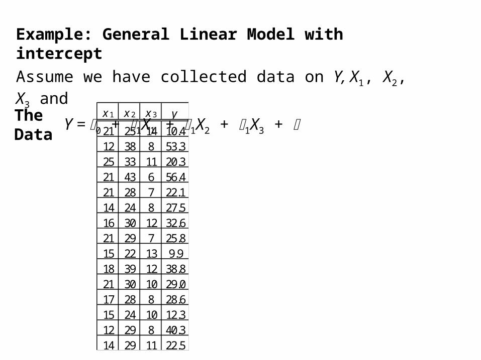
Example: General Linear Model with intercept

Assume we have collected data on Y, X1, X2, X3 and

Y = 0 + 1X1 + 1X2 + 1X3 + x 1 x 2 x 3 y

21 25 14 10.412 38 8 53.325 33 11 20.321 43 6 56.421 28 7 22.114 24 8 27.516 30 12 32.621 29 7 25.815 22 13 9.918 39 12 38.821 30 10 29.017 28 8 28.615 24 10 12.312 29 8 40.314 29 11 22.5

The Data

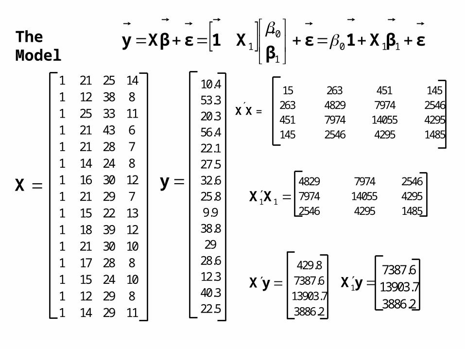
εβX1εβ

X1εβXy

110

1

01

The Model

1 21 25 141 12 38 81 25 33 111 21 43 61 21 28 71 14 24 81 16 30 121 21 29 71 15 22 131 18 39 121 21 30 101 17 28 81 15 24 101 12 29 81 14 29 11

y

X

10.453.320.356.422.127.532.625.89.938.829

28.612.340.322.5

15 263 451 145263 4829 7974 2546451 7974 14055 4295145 2546 4295 1485

XX =

429.87387.613903.73886.2

yX yX

1

7387.613903.73886.2

11XX4829 7974 25467974 14055 42952546 4295 1485

yXXX

ββ

1

1

0

ˆ

ˆˆ

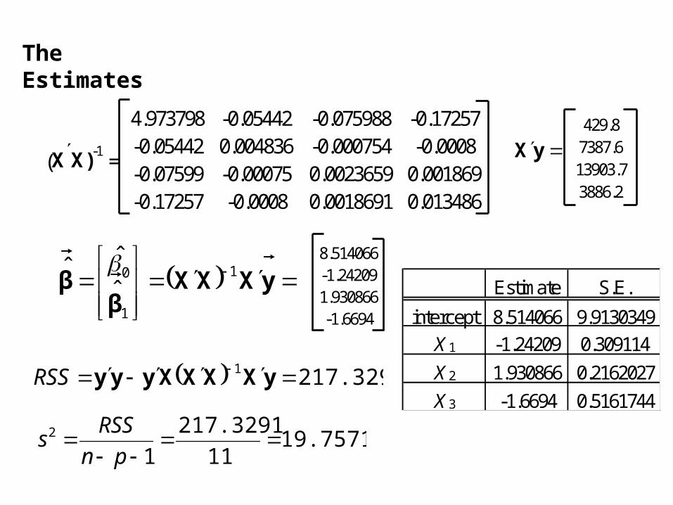
The Estimates

429.87387.613903.73886.2

yX

4.973798 -0.05442 -0.075988 -0.17257-0.05442 0.004836 -0.000754 -0.0008-0.07599 -0.00075 0.0023659 0.001869-0.17257 -0.0008 0.0018691 0.013486

(XX)-1 =

8.514066-1.242091.930866-1.6694

217.32911 yXXXXyyy

RSS

19.7571911

217.3291

12

pn

RSSs

Estimate S.E.

intercept 8.514066 9.9130349

X 1 -1.24209 0.309114

X 2 1.930866 0.2162027

X 3 -1.6694 0.5161744

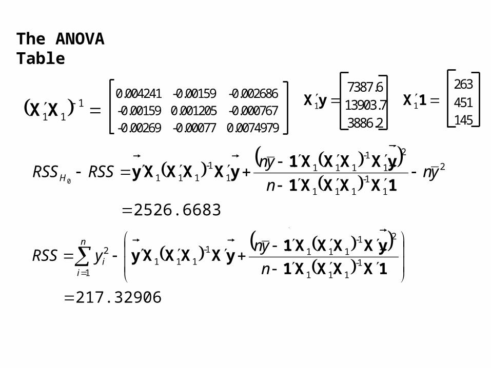
The ANOVA Table

111XX

0.004241 -0.00159 -0.002686-0.00159 0.001205 -0.000767-0.00269 -0.00077 0.0074979

yX

1

7387.613903.73886.2

263

451145

1X

1

2526.6683

2

11-

111

2

11-

1111

1-1110

ynn

ynRSSRSSH

1XXXX1

yXXXX1yXXXXy

217.32906

1-111

21-1111-

1111

2

1XXXX1

yXXXX1yXXXXy

n

ynyRSS

n

ii

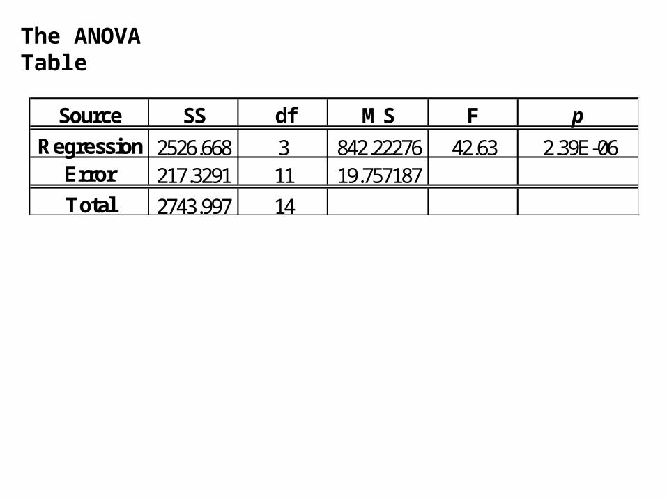
The ANOVA Table

Source SS df MS F p

Regression 2526.668 3 842.22276 42.63 2.39E-06Error 217.3291 11 19.757187

Total 2743.997 14

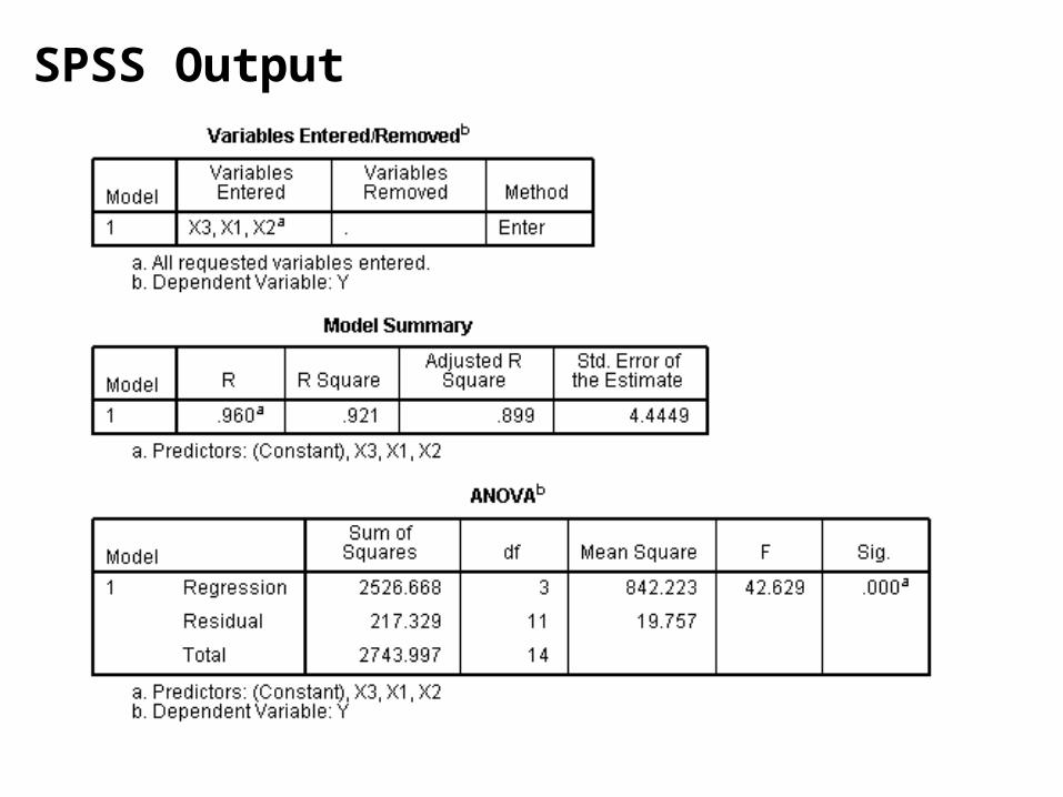
SPSS Output

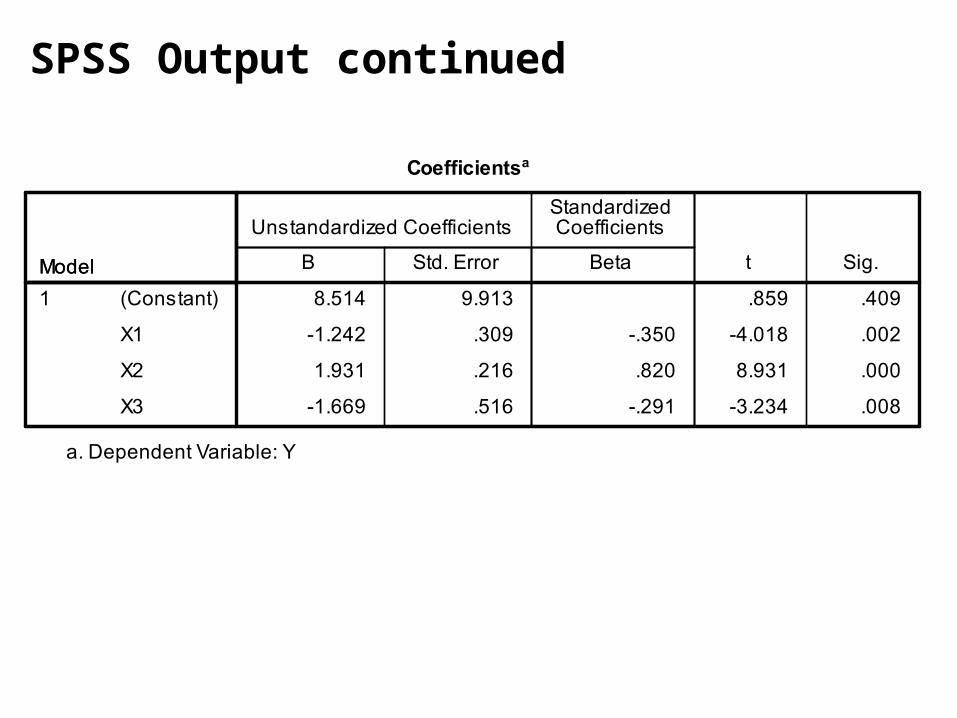
SPSS Output continued

Confidence intervals, Prediction intervals, Confidence Regions

General Linear Model

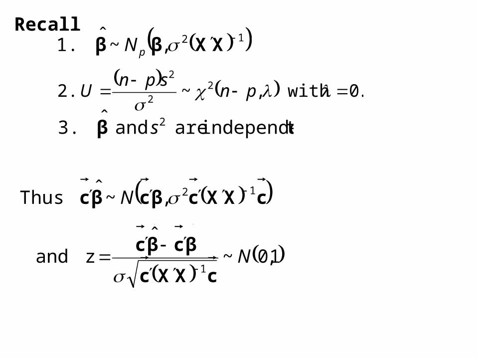
Recall

.0 with ,~ 2. 22

2

pnspn

U

12, ~ ˆ 1. XXββ

pN

tindependen are and ˆ 3. 2sβ

cXXcβcβc 12, ~ ˆ Thus N

1,0 ~

ˆz and

1N

cXXc

βcβc

Thus

pnt

s

s

pnU

zt

~ˆ

ˆ

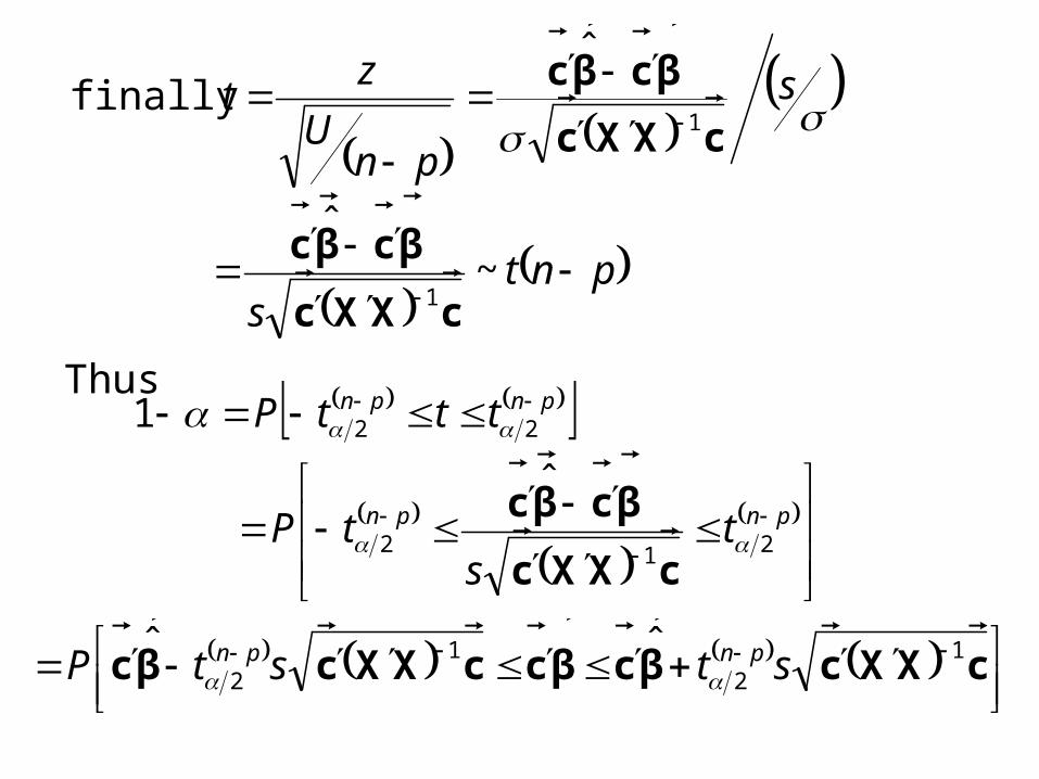
finally

1

1

cXXc

βcβc

cXXc

βcβc

pnpn

pnpn

ts

tP

tttP

212

22

ˆ

1

cXXc

βcβc

cXXcβcβccXXcβc

12

12

ˆˆ ststP pnpn

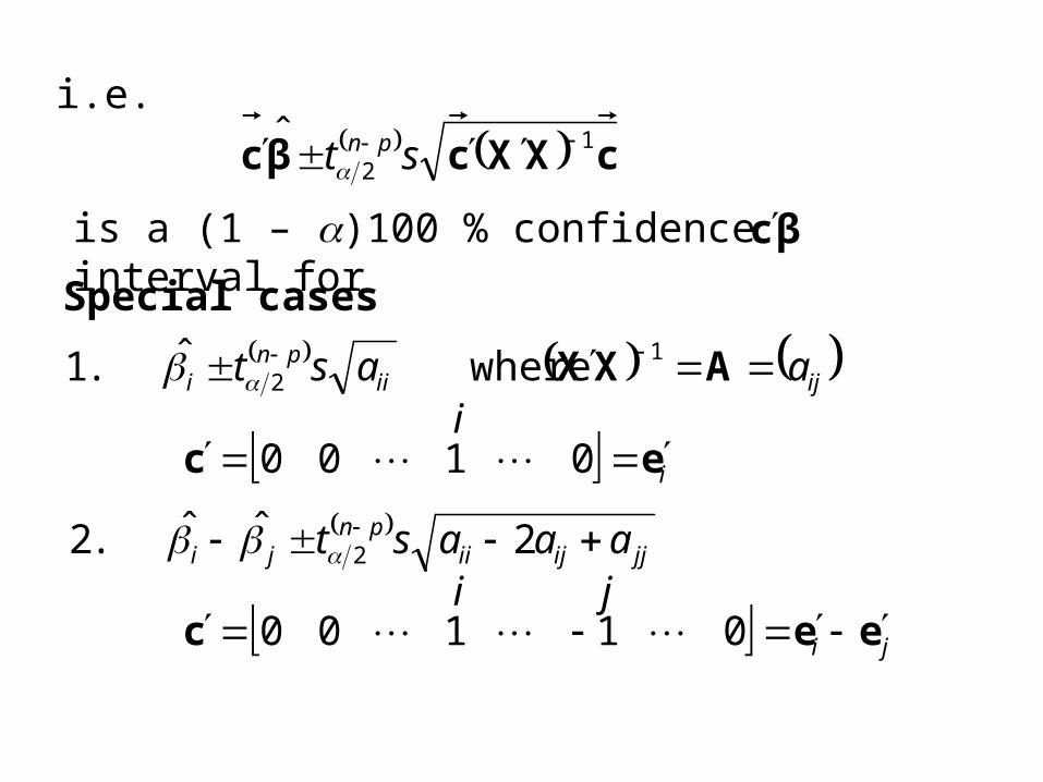
i.e. cXXcβc

12

ˆ st pn

is a (1 – )100 % confidence interval for βc

ijiipn

i aast AXX 12 whereˆ .1

2ˆˆ .2 2 jjijiipn

ji aaast

iec

0100

ji eec

01100

Special cases

i

i j

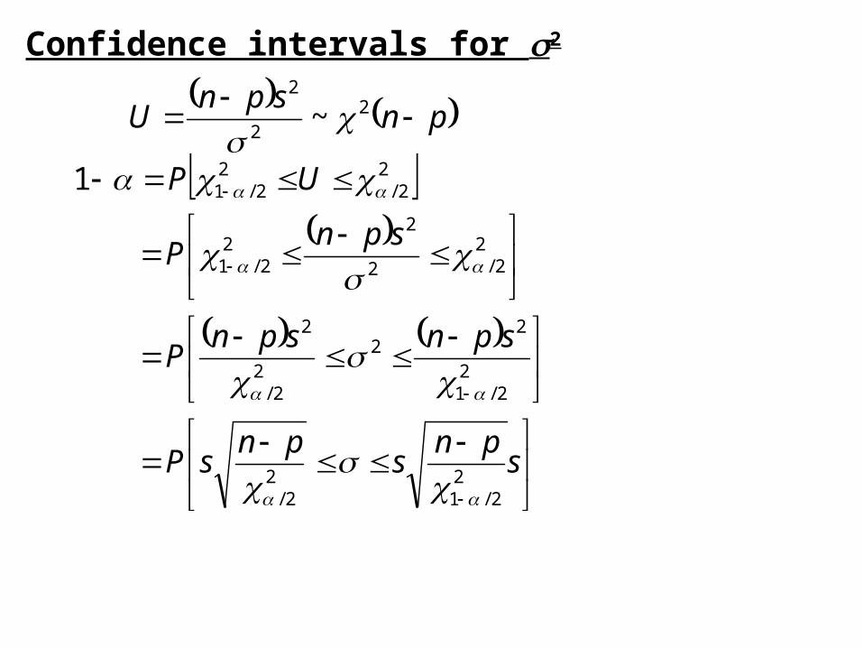
Confidence intervals for 2

~ 22

2

pnspn

U

spn

spn

sP

spnspnP

spnP

UP

22/1

22/

22/1

22

22/

2

22/2

22

2/1

22/

22/1

1

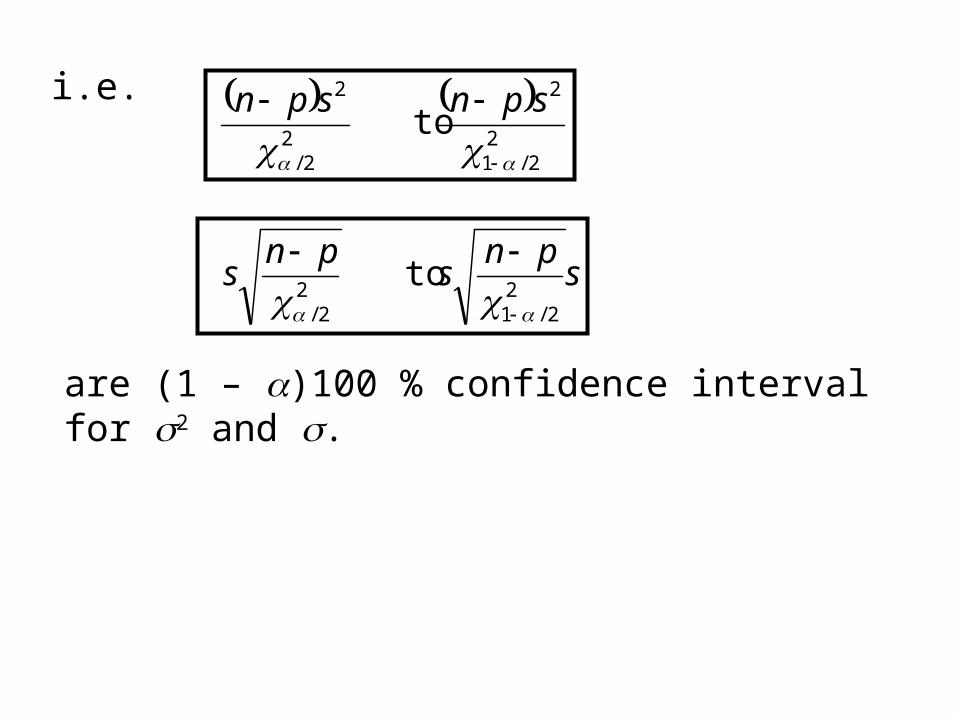
i.e.

are (1 – )100 % confidence interval for 2 and .

2

2/1

2

22/

2

to

spnspn

spn

spn

s2

2/12

2/

to

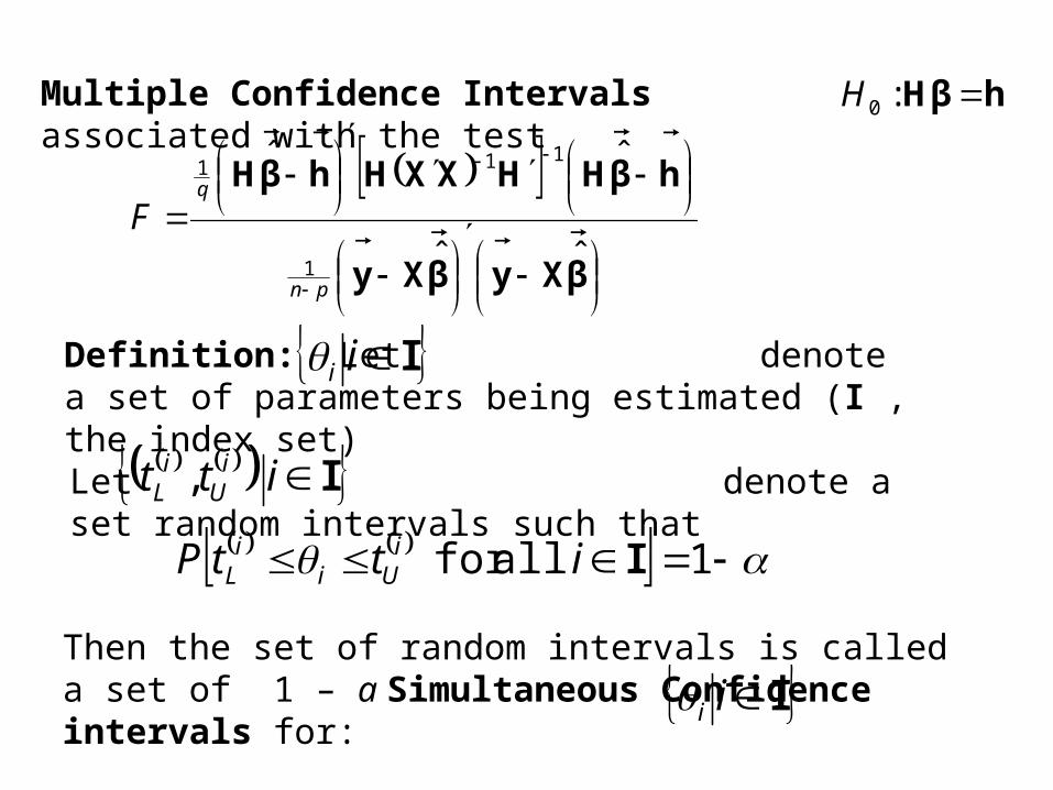
Multiple Confidence Intervals associated with the test hβH

:0H

βXyβXy

hβHHXXHhβH

ˆˆ

ˆˆ

1

111

pn

q

F

IiiDefinition: Let denote a set of parameters being estimated (I , the index set)

Then the set of random intervals is called a set of 1 – a Simultaneous Confidence intervals for:

Iitt iU

iL ,Let denote a set random intervals such that

1 allfor IittP iUi

iL

Iii

Recall cXXcβc

12

ˆ st pn

is a (1 – )100 % confidence interval for βc

However

ccXXcβc

allfor ˆ 1

2 st pn

is not a set of (1 – )100 % simultaneous confidence interval for cβc

allfor

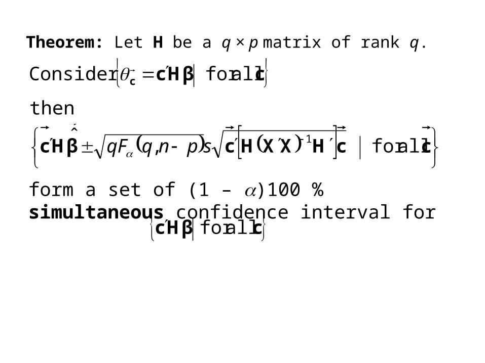
Theorem: Let H be a q × p matrix of rank q.

then

ccHXXHcβHc

allfor ,ˆ 1spnqqF

form a set of (1 – )100 % simultaneous confidence interval for cβHc

allfor

cβHcc

allfor Consider

Proof:

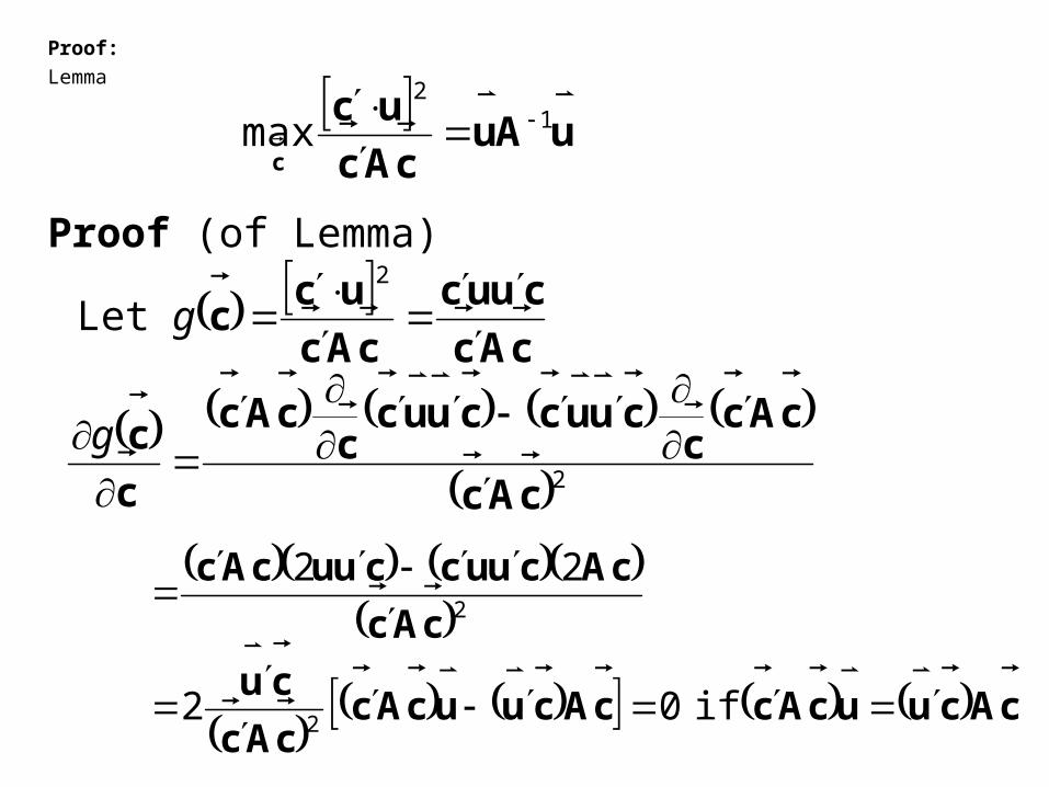
Lemma

Proof (of Lemma)

uAu

cAc

ucc

1

2

max

cAc

cuuc

cAc

ucc

2

Let g

2cAc

cAcc

cuuccuucc

cAc

c

c

g

cAcuucAccAcuucAc

cAc

cu

cAc

cAcuuccuucAc

if 02

22

2

2

or cu

cAcuAc

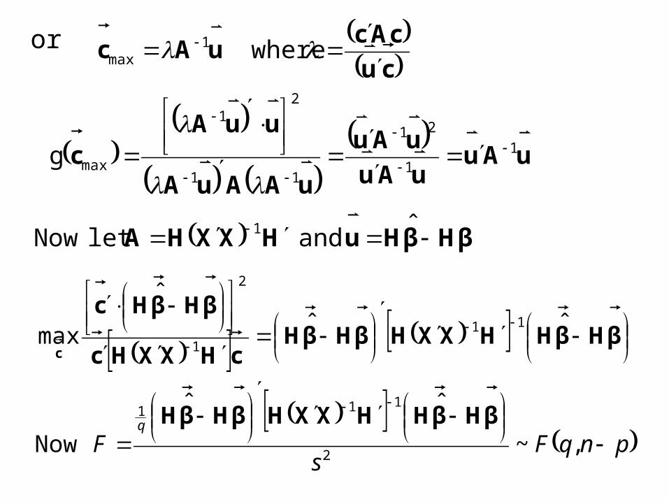
where 1max

uAuuAu

uAu

uAAuA

uuAc

1

1

21

11

21

maxg

βHβHuHXXHA ˆ and let Now 1

βHβHHXXHβHβH

cHXXHc

βHβHc

c

ˆˆ

ˆ

max11

1

2

pnqF

sF

q

,~

ˆˆ

Now2

111 βHβHHXXHβHβH

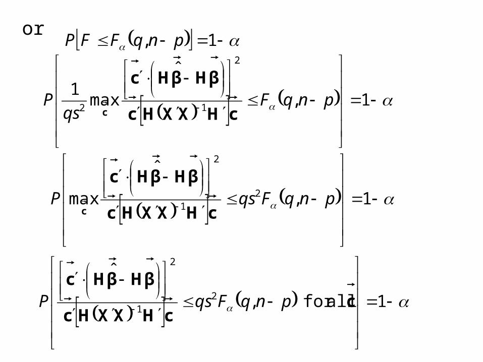
or 1, pnqFFP

1,

ˆ

max1

1

2

2pnqF

qsP

cHXXHc

βHβHc

c

1,

ˆ

max 21

2

pnqFqsPcHXXHc

βHβHc

c

1 allfor ,

ˆ

21

2

ccHXXHc

βHβHc

pnqFqsP

or

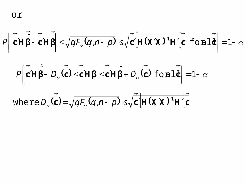
1 allfor ,ˆ 1 ccHXXHcβHcβHc

spnqqFP

1 allfor ˆˆ ccβHcβHccβHc

DDP

cHXXHcc 1, where spnqqFD

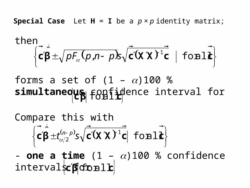
Special Case Let H = I be a p × p identity matrix;

then

ccXXcβc

allfor ,ˆ 1spnppF

forms a set of (1 – )100 % simultaneous confidence interval for cβc

allfor

Compare this with

ccXXcβc

allfor ˆ 1

2 st pn

- one a time (1 – )100 % confidence intervals for cβc

allfor

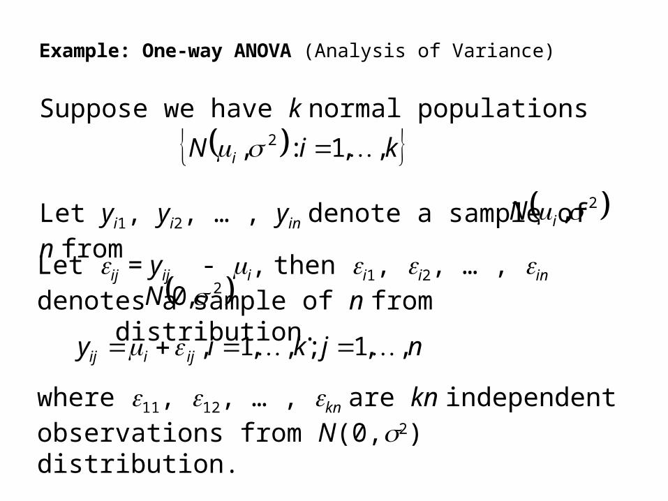
Example: One-way ANOVA (Analysis of Variance)

Suppose we have k normal populations

Let yi1, yi2, … , yin denote a sample of n from

kiN i ,,1:, 2

2,iN

Let ij = yij - i, then i1, i2, … , in denotes a sample of n from distribution. 2,0 N

njkiy ijiij ,,1;,,1,

where 11, 12, … , kn are kn independent observations from N(0,2) distribution.

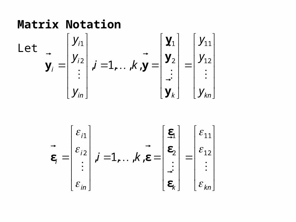
Matrix Notation

Let

knkin

i

i

i

y

y

y

ki

y

y

y

12

11

2

1

2

1

,,,1,

y

y

y

yy

knkin

i

i

i ki

12

11

2

1

2

1

,,,1,

ε

ε

ε

εε

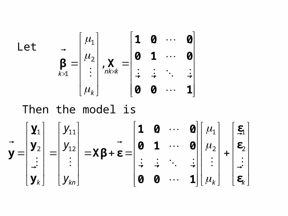
Let

100

010

001

Xβ

knk

k

k,2

1

1

kkknk y

y

y

ε

ε

ε

100

010

001

εXβ

y

y

y

y

2

1

2

1

12

11

2

1

Then the model is

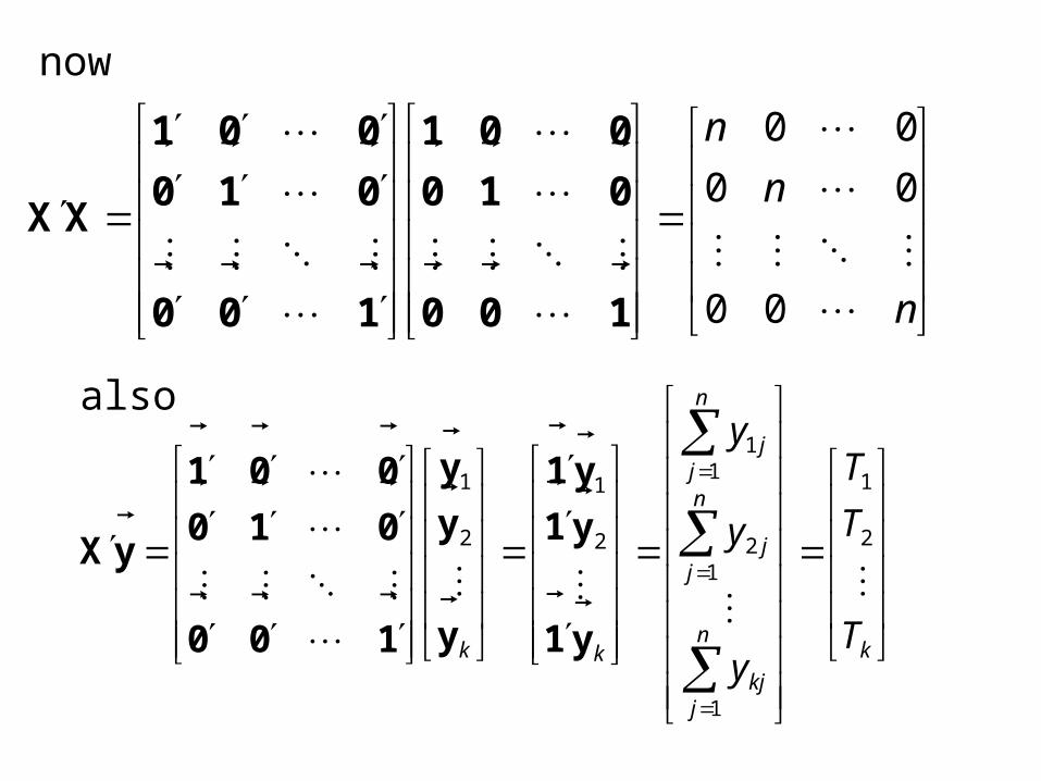
now

n

n

n

00

00

00

100

010

001

100

010

001

XX

kn

jkj

n

jj

n

jj

kk T

T

T

y

y

y

2

1

1

12

11

2

1

2

1

y1

y1

y1

y

y

y

100

010

001

yX

also

also

n

n

n

n

n

n

1

1

11

1

00

00

00

00

00

00

XX

kkn

n

n

k y

y

y

T

T

T

2

1

2

1

1

1

1

12

1

00

00

00

ˆ

ˆ

ˆ

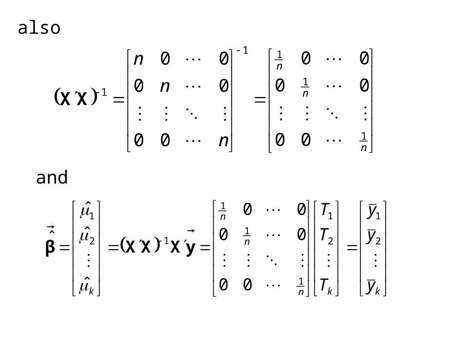
ˆ yXXXβ

and

Finally the UMVU of 2 is

knk

SS

n

Ty

yTy

s

k

i

ik

i

n

jijknk

k

iii

k

i

n

jijknk

knk

Error

1

2

1 1

21

11 1

21

12

ˆ yXβyy

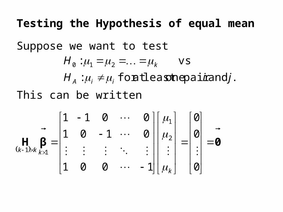
Testing the Hypothesis of equal mean

Suppose we want to test

This can be written

. and pair oneleast at for :

vs: 210

jiH

H

iiA

k

0βH

0

0

0

1001

0101

0011

2

1

11

k

kkk

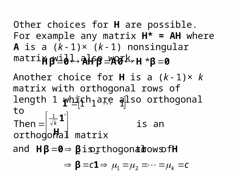
Other choices for H are possible. For example any matrix H* = AH where A is a (k - 1)× (k - 1) nonsingular matrix will also work.

Another choice for H is a (k - 1)× k matrix with orthogonal rows of length 1 which are also orthogonal to

0βH0AβAH0βH

*

111 1

Then is an orthogonal matrix

H

1

k1

and

cc k

21

of rows toorthogonal is

1β

Hβ0βH

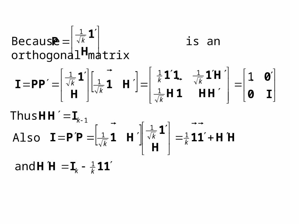
Because is an orthogonal matrix

H

1P

k

1

I0

0

HH1H

H111H1

H

1PPI

1

1

111

1

k

kk

kk

1 Thus kIHH

Also 11

1 HH11H

1H1PPI

k

kk

11IHH

kk1 and

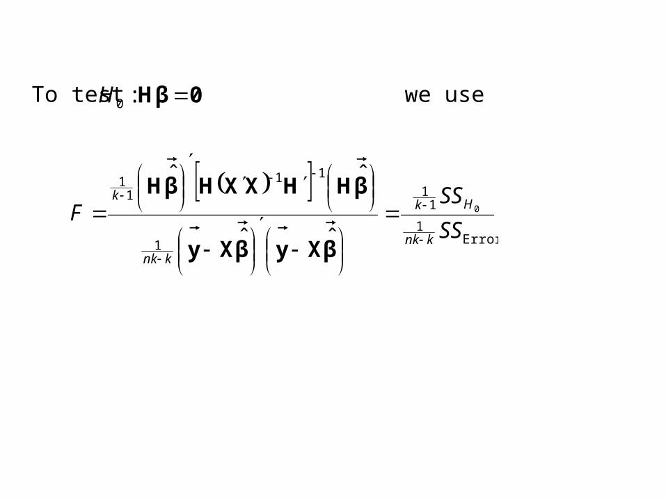
To test we use0βH

:0H

Error

1

11

1

111

1

0

ˆˆ

ˆˆ

SS

SSF

knk

Hk

knk

k

βXyβXy

βHHXXHβH

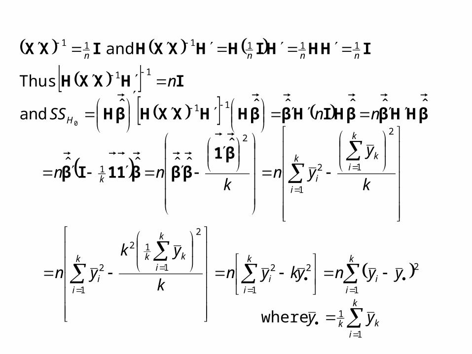
IHHHIHHXXHIXX nnnn111111 and

IHXXH n 11 Thus

βHHββHIHββHHXXHβH ˆˆˆˆˆˆ and11

0

nnSSH

k

y

ynk

nn

k

ikk

iik

2

1

1

2

2

1

ˆˆˆˆˆ

β1βββ11Iβ

k

ii

k

ii

k

ikkk

ii yynykyn

k

yk

yn1

22

1

2

2

1

12

1

2

k

ikk yy

1

1 where

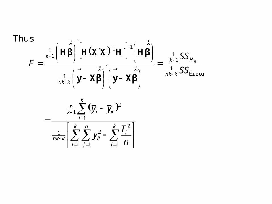
Thus

Error

1

11

1

111

1

0

ˆˆ

ˆˆ

SS

SSF

knk

Hk

knk

k

βXyβXy

βHHXXHβH

k

i

ik

i

n

jijknk

k

iik

n

n

Ty

yy

1

2

1 1

21

1

21

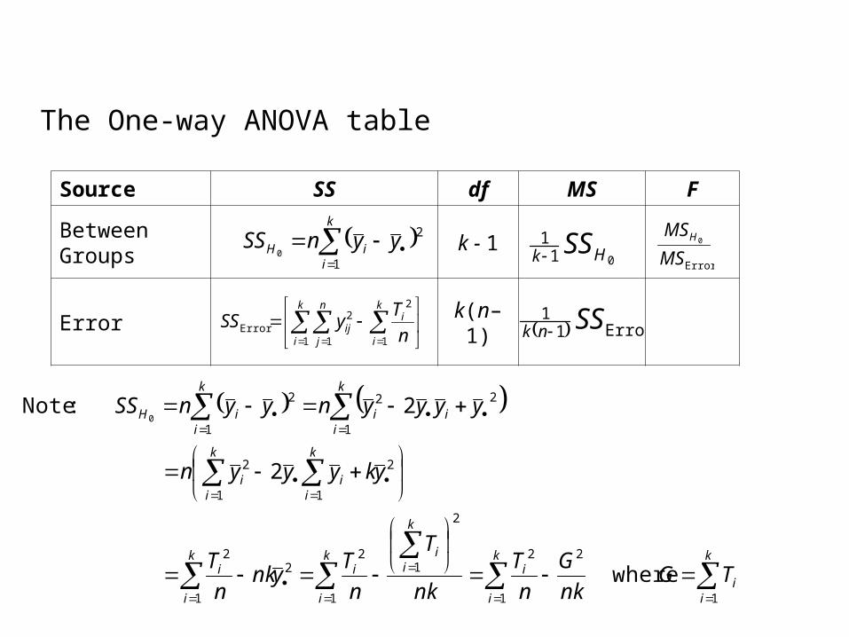
The One-way ANOVA table

Source SS df MS F

Between Groups k - 1

Error k(n– 1)

k

i

ik

i

n

jij n

TySS

1

2

1 1

2Error

k

iiH yynSS

1

2

001

1Hk SS

Error11 SSnk

Error

0

MS

MSH

k

ii

k

i

i

k

iik

i

ik

i

i

k

ii

k

ii

k

iii

k

iiH

TGnk

G

n

T

nk

T

n

Tynk

n

T

ykyyyn

yyyynyynSS

1

2

1

2

2

1

1

22

1

2

2

11

2

1

22

1

2

where

2

2 :Note0

Simultaneous Confidence intervals related to the test for:

cHXXHcβHc 1,ˆ spnqqF

hβH

:0H

cβbβHc

allfor

parameters for the sCI' ussimultaneo %1001 ofset a form

01H1Hc1bbHc

since 0 and :Notenknkq and 1 also

Thus bXXbβb

1,11ˆ sknkkFk

0 such that allfor

parameters for the sCI' ussimultaneo %1001 ofset a form

1bbβb

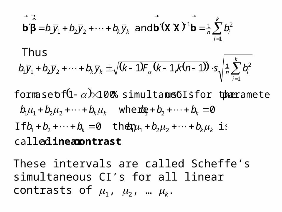
parameters for the sCI' ussimultaneo %1001 ofset a form

These intervals are called Scheffe‘s simultaneous CI’s for all linear contrasts of 1, 2, … k.

k

iinkk bybybyb

1

2112211 and ˆ bXXbβb

Thus

k

iinkk bsnkkFkybybyb

1

212211 1,11

0 where 212211 kkk bbbbbb

. a called

is then 0 If 221121

contrastlinearkkk bbbbbb

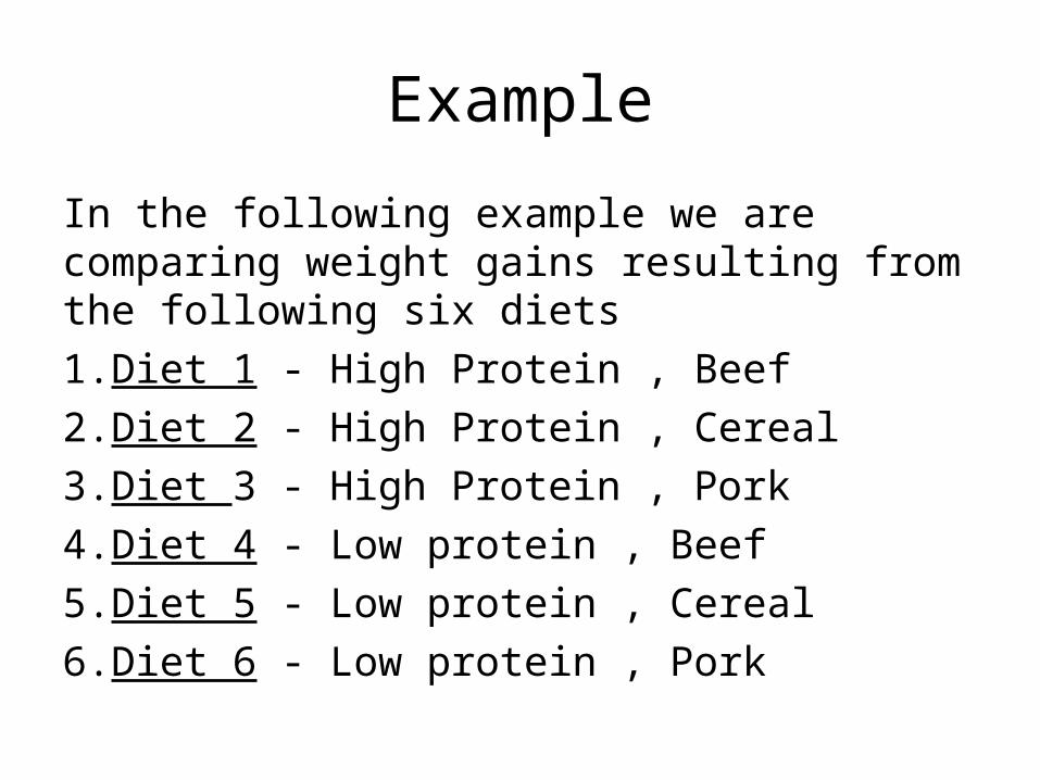
Example

In the following example we are comparing weight gains resulting from the following six diets

1.Diet 1 - High Protein , Beef

2.Diet 2 - High Protein , Cereal

3.Diet 3 - High Protein , Pork

4.Diet 4 - Low protein , Beef

5.Diet 5 - Low protein , Cereal

6.Diet 6 - Low protein , Pork

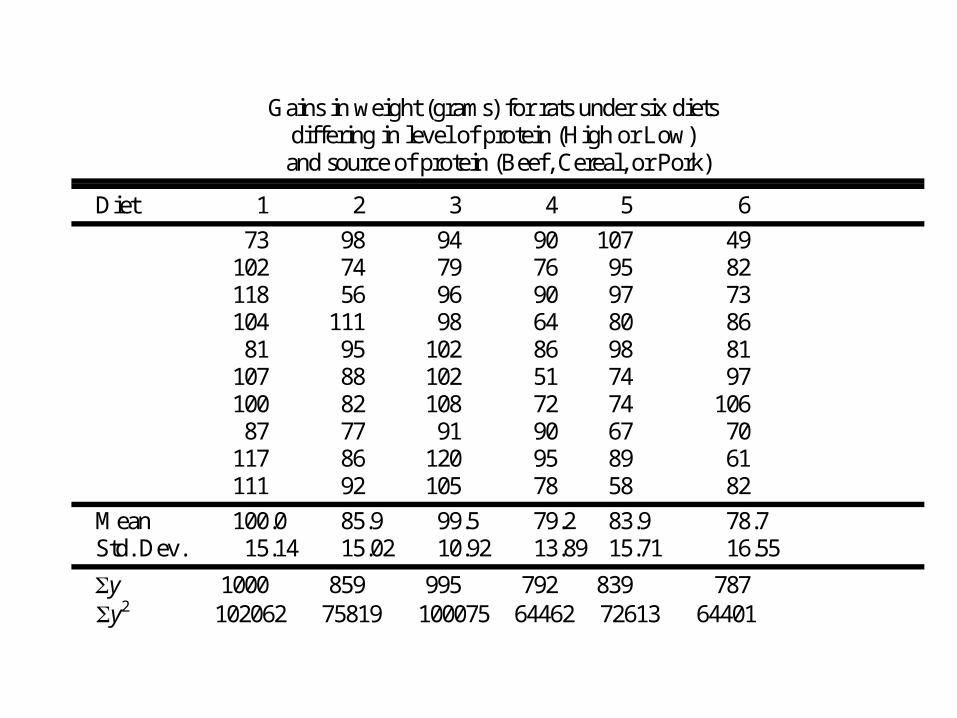
Gains in weight (grams) for rats under six diets differing in level of protein (High or Low) and source of protein (Beef, Cereal, or Pork)

Diet 1 2 3 4 5 6

73 98 94 90 107 49 102 74 79 76 95 82 118 56 96 90 97 73 104 111 98 64 80 86 81 95 102 86 98 81 107 88 102 51 74 97 100 82 108 72 74 106 87 77 91 90 67 70 117 86 120 95 89 61 111 92 105 78 58 82

Mean 100.0 85.9 99.5 79.2 83.9 78.7 Std. Dev. 15.14 15.02 10.92 13.89 15.71 16.55

y 1000 859 995 792 839 787 y2 102062 75819 100075 64462 72613 64401

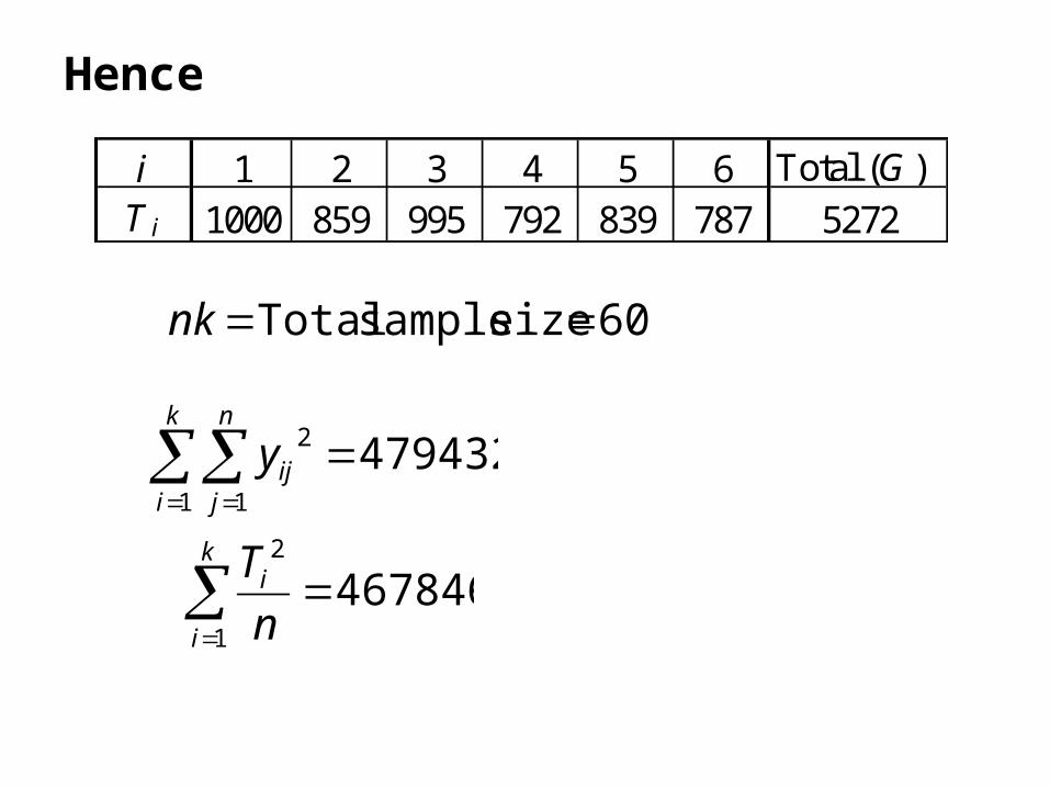
Hence

4794321 1

2

k

i

n

jijy

60 size sample Total nk

4678461

2

k

i

i

n

T

i 1 2 3 4 5 6 Total (G )T i 1000 859 995 792 839 787 5272

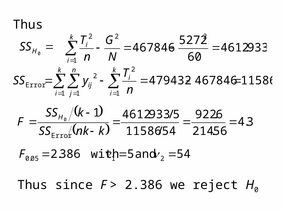
Thus

115864678464794321

2

1 1

2Error

k

i

ik

i

n

jij n

TySS

0HSS 933.4612

60

5272467846

2

1

22

k

i

i

N

G

n

T

3.4

56.214

6.922

54/11586

5/933.46121

Error

0

knkSS

kSSF H

54 and 5 with 386.2 2105.0 F

Thus since F > 2.386 we reject H0

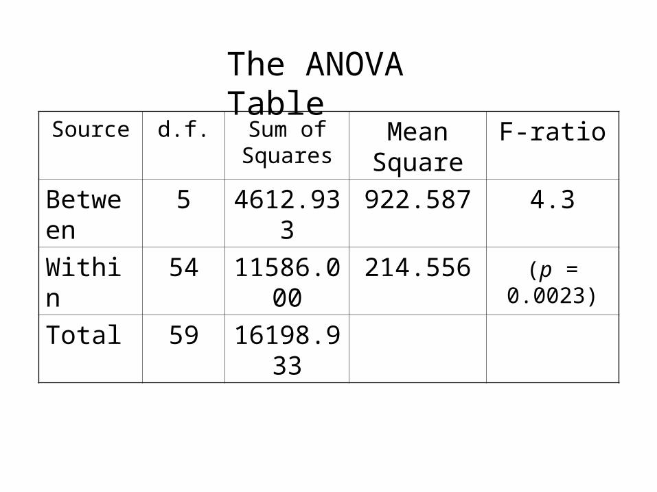
Source d.f. Sum of Squares

Mean Square

F-ratio

Between 5 4612.933 922.587 4.3

Within 54 11586.000 214.556 (p = 0.0023)

Total 59 16198.933

The ANOVA Table

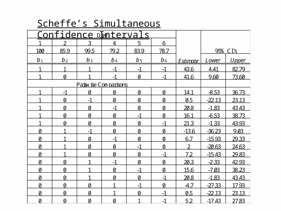
Scheffe’s Simultaneous Confidence Intervals

1 2 3 4 5 6100 85.9 99.5 79.2 83.9 78.7

b 1 b 2 b 3 b 4 b 5 b 6 Lower Upper

1 1 1 -1 -1 -1 43.6 4.41 82.791 0 1 -1 0 -1 41.6 9.60 73.60

1 -1 0 0 0 0 14.1 -8.53 36.731 0 -1 0 0 0 0.5 -22.13 23.131 0 0 -1 0 0 20.8 -1.83 43.431 0 0 0 -1 0 16.1 -6.53 38.731 0 0 0 0 -1 21.3 -1.33 43.930 1 -1 0 0 0 -13.6 -36.23 9.030 1 0 -1 0 0 6.7 -15.93 29.330 1 0 0 -1 0 2 -20.63 24.630 1 0 0 0 -1 7.2 -15.43 29.830 0 1 -1 0 0 20.3 -2.33 42.930 0 1 0 -1 0 15.6 -7.03 38.230 0 1 0 0 -1 20.8 -1.83 43.430 0 0 1 -1 0 -4.7 -27.33 17.930 0 0 1 0 -1 0.5 -22.13 23.130 0 0 0 1 -1 5.2 -17.43 27.83

Pairwise Comparisons

Diet

Estimate

95% CI's