Statistics / Econometrics: Hypothesis Testing

Course : Introductory Econometrics / Statistics : HC43B.A. Hons Economics, Semester IV / III

Delhi University

Course Instructor:

Siddharth RathoreAssistant Professor

Economics Department, Gargi College

Siddharth Rathore

487

APPENDIX DSTATISTICAL INFERENCE:

ESTIMATION ANDHYPOTHESIS TESTING

Equipped with the knowledge of probability; random variables; probabilitydistributions; and characteristics of probability distributions, such as expectedvalue, variance, covariance, correlation, and conditional expectation, in thisappendix we are now ready to undertake the important task of statisticalinference. Broadly speaking, statistical inference is concerned with drawingconclusions about the nature of some population (e.g., the normal) on the basisof a random sample that has supposedly been drawn from that population.Thus, if we believe that a particular sample has come from a normal populationand we compute the sample mean and sample variance from that sample, wemay want to know what the true (population) mean is and what the variance ofthat population may be.

D.1 THE MEANING OF STATISTICAL INFERENCE1

As noted previously, the concepts of population and sample are extremely impor-tant in statistics. Population, as defined in Appendix A, is the totality of all possibleoutcomes of a phenomenon of interest (e.g., the population of New York City). Asample is a subset of a population (e.g., the people living in Manhattan, which isone of the five boroughs of the city). Statistical inference, loosely speaking, is thestudy of the relationship between a population and a sample drawn from thatpopulation. To understand what this means, let us consider a concrete example.

1Broadly speaking, there are two approaches to statistical inference, Bayesian and classical. Theclassical approach, as propounded by statisticians Neyman and Pearson, is generally the ap-proach that a beginning student in statistics first encounters. Although there are basic philosophi-cal differences in the two approaches, there may not be gross differences in the inferences that result.

guj75845_appD.qxd 4/16/09 12:42 PM Page 487

The Pink Professor

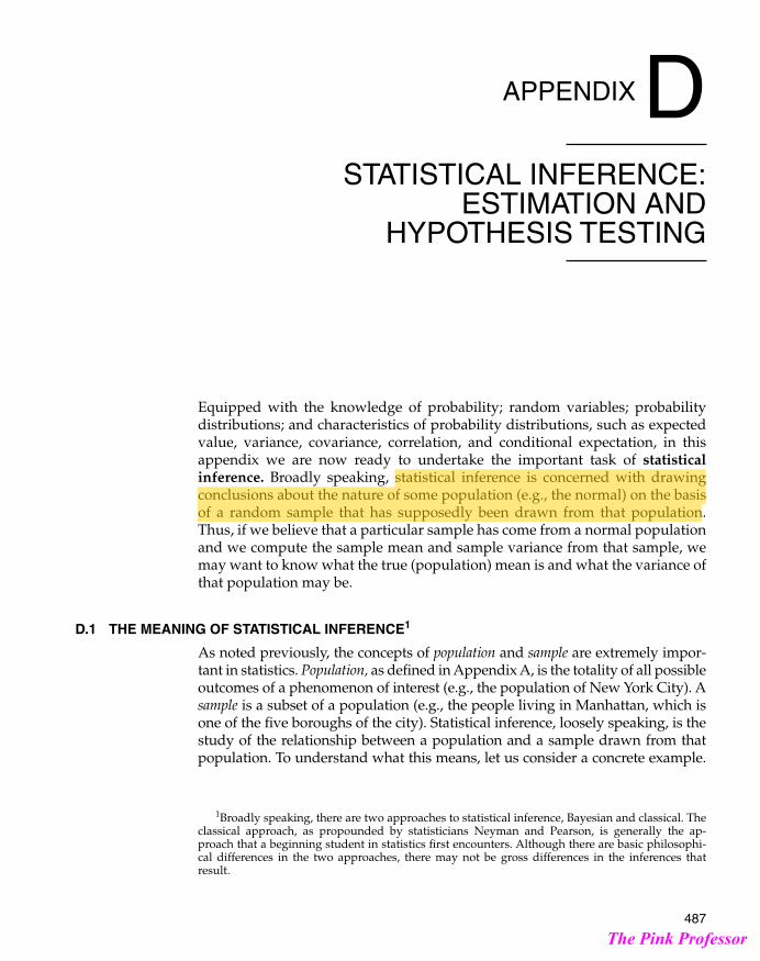
Table D-1 gives data on the price to earnings ratio—the famous P/E ratio—for28 companies listed on the New York Stock Exchange (NYSE) for February 2,2004 (at about 3 p.m.).2 Assume that this is a random sample from the universe(population) of stocks listed on the NYSE, some 3000 or so. The P/E ratio of27.96 for Alcoa (AA) listed in this table, for example, means that on that day thestock was selling at about 28 times its annual earnings. The P/E ratio is one ofthe key indicators for investors in the stock market.

Suppose our primary interest is not in any single P/E ratio, but in the aver-age P/E ratio in the entire population of the NYSE listed stocks. Since we canobtain data on the P/E ratios of all the stocks listed on the NYSE, in principle,we can easily compute the average P/E ratio. In practice, that would be time-consuming and expensive. Could we use the data given in Table D-1 to com-pute the average P/E ratio of the 28 companies listed in this table and use this(sample) average as an estimate of the average P/E ratio in the entire popula-tion of the stocks listed on the NYSE? Specifically, if we let X = P/E ratio of astock and = the average P/E ratio of the 28 stocks given in Table D-1, canwe tell what the expected P/E ratio, E(X), is in the NYSE population as a whole?This process of generalizing from the sample value (e.g., ) to the population value(e.g., E[X]) is the essence of statistical inference. We will now discuss this topic insome detail.

X

X

488 APPENDIXES

PRICE TO EARNINGS (P/E) RATIOS OF 28 COMPANIES ON THE NEW YORK STOCK EXCHANGE (NYSE)

Company P/E Company P/E

AA 27.96 INTC 36.02AXP 22.90 IBM 22.94T 8.30 JPM 12.10BA 49.78 JNJ 22.43CAT 24.68 MCD 22.13C 14.55 MRK 16.48KO 28.22 MSFT 33.75DD 28.21 MMM 26.05EK 34.71 MO 12.21XOM 12.99 PG 24.49GE 21.89 SBC 14.87GM 9.86 UTX 14.87HD 20.26 WMT 27.84HON 23.36 DIS 37.10Mean = 23.25, variance = 90.13, standard deviation = 9.49

Source: www.stockselector.com.

TABLE D-1

2Since the price of the stock varies from day to day, the P/E ratio will vary from day to day, eventhough the earnings do not change. The stocks given in this table are members of the so-calledDow 30. In reality stock prices change very frequently when the stock market is open, but mostnewspapers quote the P/E ratios as of the end of the business day.

guj75845_appD.qxd 4/16/09 12:42 PM Page 488

The Pink Professor

D.2 ESTIMATION AND HYPOTHESIS TESTING:TWIN BRANCHESOF STATISTICAL INFERENCE

From the preceding discussion it can be seen that statistical inference proceedsalong the following lines. There is some population of interest, say, the stockslisted on the NYSE, and we are interested in studying some aspect of thispopulation, say, the P/E ratio. Of course, we may not want to study each andevery P/E ratio, but only the average P/E ratio. Since collecting information onall the NYSE P/E ratios needed to compute the average P/E ratio is expensiveand time-consuming, we may obtain a random sample of only a few stocks toget the P/E ratio of each of these sampled stocks and compute the sampleaverage P/E ratio, say, . is an estimator, also known as a (sample) statis-tic, of the population average P/E ratio, E(X), which is called the (population)parameter. (Refer to the discussion in Appendix B). For example, the meanand variance are the parameters of the normal distribution. A particular nu-merical value of the estimator is called an estimate (e.g., an value of 23).Thus, estimation is the first step in statistical inference. Having obtained anestimate of a parameter, we next need to find out how good that estimate is,for an estimate is not likely to equal the true parameter value. If we obtain twoor more random samples of 28 stocks each and compute for each of thesesamples, the two estimates will probably not be the same. This variation inestimates from sample to sample is known as sampling variation or samplingerror.3 Are there any criteria by which we can judge the “goodness” of an esti-mator? In Section D.4 we discuss some of the commonly used criteria to judgethe goodness of an estimator.

Whereas estimation is one side of statistical inference, hypothesis testing isthe other. In hypothesis testing we may have prior judgment or expectationabout what value a particular parameter may assume. For example, priorknowledge or an expert opinion tells us that the true average P/E ratio in thepopulation of NYSE stocks is, say, 20. Suppose a particular random sample of28 stocks gives this estimate as 23. Is this value of 23 close to the hypothesizedvalue of 20? Obviously, the number 23 is different from the number 20. But theimportant question here is this: Is 23 statistically different from 20? We know thatbecause of sampling variation there is likely to be a difference between a(sample) estimate and its population value. It is possible that statistically thenumber 23 may not be very different from the number 20, in which case wemay not reject the hypothesis that the true average P/E ratio is 20. But how dowe decide that? This is the essence of the topic of hypothesis testing, which wewill discuss in Section D.5.

With these preliminaries, let us examine the twin topics of estimation andhypothesis testing in some detail.

X

X

XX

APPENDIX D: STATISTICAL INFERENCE: ESTIMATION AND HYPOTHESIS TESTING 489

3Notice that this sampling error is not deliberate, but it occurs because we have a random sample and the elements included in the sample will vary from sample to sample. This is inevitablein any analysis based on a sample.

guj75845_appD.qxd 4/16/09 12:42 PM Page 489

The Pink Professor

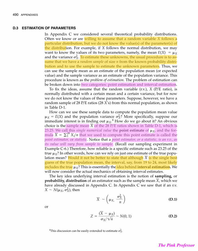
D.3 ESTIMATION OF PARAMETERS

In Appendix C we considered several theoretical probability distributions.Often we know or are willing to assume that a random variable X follows aparticular distribution, but we do not know the value(s) of the parameter(s) ofthe distribution. For example, if X follows the normal distribution, we maywant to know the values of its two parameters, namely, the mean E(X)and the variance . To estimate these unknowns, the usual procedure is to as-sume that we have a random sample of size n from the known probability distri-bution and to use the sample to estimate the unknown parameters. Thus, wecan use the sample mean as an estimate of the population mean (or expectedvalue) and the sample variance as an estimate of the population variance. Thisprocedure is known as the problem of estimation. The problem of estimation canbe broken down into two categories: point estimation and interval estimation.

To fix the ideas, assume that the random variable (r.v.), X (P/E ratio), isnormally distributed with a certain mean and a certain variance, but for nowwe do not know the values of these parameters. Suppose, however, we have arandom sample of 28 P/E ratios (28 X’s) from this normal population, as shownin Table D-1.

How can we use these sample data to compute the population mean value= E(X) and the population variance More specifically, suppose our

immediate interest is in finding out .4 How do we go about it? An obviouschoice is the sample mean of the 28 P/E ratios shown in Table D-1, which is23.25. We call this single numerical value the point estimate of , and the for-mula that we used to compute this point estimate is called thepoint estimator, or statistic. Notice that a point estimator, or a statistic, is an r.v., asits value will vary from sample to sample. (Recall our sampling experiment inExample C-6.) Therefore, how reliable is a specific estimate such as 23.25 of thetrue ? In other words, how can we rely on just one estimate of the true popu-lation mean? Would it not be better to state that although is the single bestguess of the true population mean, the interval, say, from 19 to 24, most likelyincludes the true ? This is essentially the idea behind interval estimation. Wewill now consider the actual mechanics of obtaining interval estimates.

The key idea underlying interval estimation is the notion of sampling, orprobability, distribution of an estimator such as the sample mean , which wehave already discussed in Appendix C. In Appendix C we saw that if an r.v.

then

(D.1)

or

(D.2)Z =

(X - �X)�X>1n

' N(0, 1)

X ' a�X, �2

X

nb

X ' N(�X, �2X),

X

�X

X�X

X = g281 Xi>n

�X

X�X

�2X?�X

�2X

= �X

490 APPENDIXES

4This discussion can be easily extended to estimate .�2X

guj75845_appD.qxd 4/16/09 12:42 PM Page 490

The Pink Professor

That is, the sampling distribution of the sample mean also follows the normaldistribution with the stated parameters.5

As pointed out in Appendix C, is not generally known, but if we use itsestimator , then we know that

(D.3)

follows the t distribution with (n - 1) degrees of freedom (d.f.).To see how Equation (D.3) helps us to obtain an interval estimation of the

of our P/E example, note that we have a total of 28 observations and, therefore,27 d.f. Now if we consult the t table (Table E-2) given in Appendix E, we noticethat for 27 d.f.,

(D.4)

as shown in Figure D-1. That is, for 27 d.f., the probability is 0.95 (or 95 percent)that the interval (-2.052, 2.052) will include the t value computed from Eq. (D.3).6

These t values, as we will see shortly, are known as critical t values; they showwhat percentage of the area under the t distribution curve (see Figure D-1) liesbetween those values (note that the total area under the curve is 1); t = -2.052is called the lower critical t value and t = 2.052 is called the upper critical t value.

Now substituting the t value from Eq. (D.3) into Eq. (D.4), we obtain

(D.5)

Simple algebraic manipulation will show that Equation (D.5) can be expressedequivalently as

(D.6)PaX - 2.052Sx

1n… �X … X + 2.052

Sx

1nb = 0.95

Pa -2.052 …

(X - �X)Sx>1n

… 2.052b

P(-2.052 … t … 2.052) = 0.95

�X

t =

(X - �X)Sx>1n

S2x = g (Xi - X)2

>(n - 1)�2

X

X

APPENDIX D: STATISTICAL INFERENCE: ESTIMATION AND HYPOTHESIS TESTING 491

2.5%

−2.052

2.5%

2.0520

The t distribution for 27 d.f.FIGURE D-1

5Note that if X does not follow the normal distribution, will follow the normal distribution àla the central limit theorem if n, the sample size, is sufficiently large.

6Needless to say, these values will depend on the d.f. as well as on the level of probability used.For example, for the same d.f. P(-2.771 … t … 2.771) = 0.99.

X

guj75845_appD.qxd 4/16/09 12:42 PM Page 491

The Pink Professor

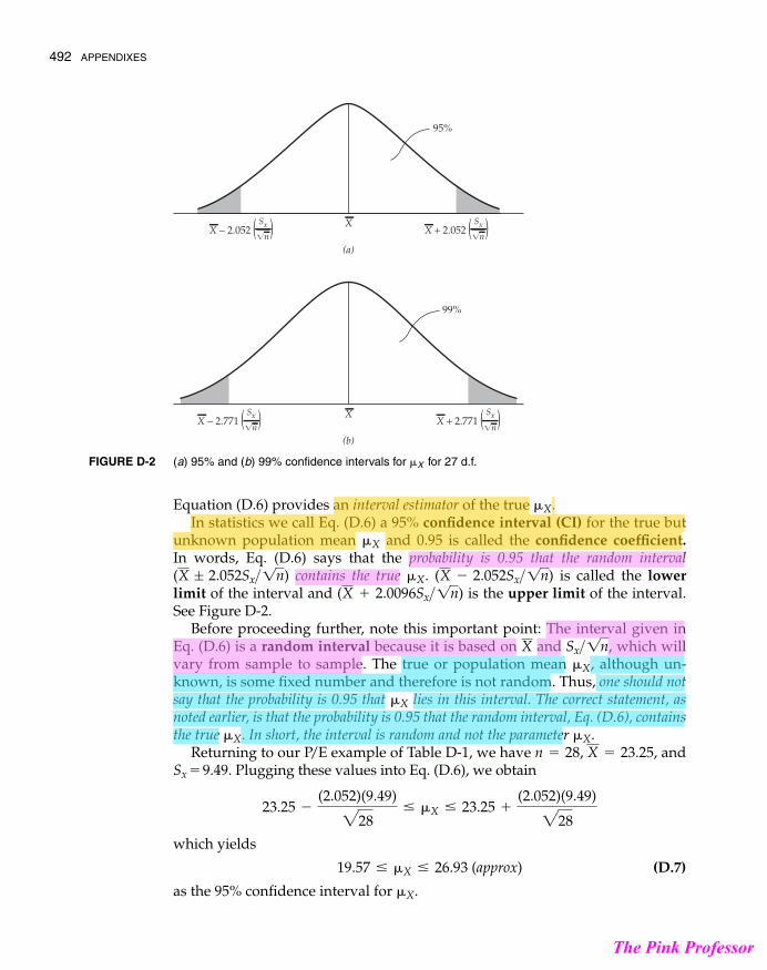
Equation (D.6) provides an interval estimator of the true .In statistics we call Eq. (D.6) a 95% confidence interval (CI) for the true but

unknown population mean and 0.95 is called the confidence coefficient.In words, Eq. (D.6) says that the probability is 0.95 that the random interval

contains the true . is called the lowerlimit of the interval and is the upper limit of the interval.See Figure D-2.

Before proceeding further, note this important point: The interval given inEq. (D.6) is a random interval because it is based on and , which willvary from sample to sample. The true or population mean , although un-known, is some fixed number and therefore is not random. Thus, one should notsay that the probability is 0.95 that lies in this interval. The correct statement, asnoted earlier, is that the probability is 0.95 that the random interval, Eq. (D.6), containsthe true . In short, the interval is random and not the parameter .

Returning to our P/E example of Table D-1, we have , and Sx = 9.49. Plugging these values into Eq. (D.6), we obtain

which yields

(D.7)

as the 95% confidence interval for .�X

19.57 … �X … 26.93 (approx)

23.25 -

(2.052)(9.49)

228… �X … 23.25 +

(2.052)(9.49)

228

n = 28, X = 23.25�X�X

�X

�X

Sx>1nX

(X + 2.0096Sx>1n)(X - 2.052Sx>1n)�X(X ; 2.052Sx>1n)

�X

�X

492 APPENDIXES

X

(a)

95%

X

(b)

99%

X − 2.052 Sx

�nX + 2.052

Sx

�n

X − 2.771 Sx

�nX + 2.771

Sx

�n

(a) 95% and (b) 99% confidence intervals for for 27 d.f.�XFIGURE D-2

guj75845_appD.qxd 4/16/09 12:42 PM Page 492

The Pink Professor

Equation (D.7) says, in effect, that if we construct intervals like Eq. (D.7),say, 100 times, then 95 out of 100 such intervals will include the true .7

Incidentally, note that for our P/E example the lower limit of the interval is 19.57and the upper limit is 26.93.

Thus, interval estimation, in contrast to point estimation (such as 23.25), providesa range of values that will include the true value with a certain degree of confidenceor probability (such as 0.95). If we have to give one best estimate of the truemean, it is the point estimate 23.25, but if we want to be less precise we cangive the interval (19.57 to 26.93) as the range that most probably includes thetrue mean value with a certain degree of confidence (95 percent in the presentinstance).

More generally, suppose X is an r.v. with some probability distribution func-tion (PDF). Suppose further that we want to estimate a parameter of this distri-bution, say, its mean value . Toward that end, we obtain a random sample ofn values, , and compute two statistics (or estimators) L and Ufrom this sample such that

(D.8)

That is, the probability is that the random interval from L to U containsthe true . L is called the lower limit of the interval and U is called the upperlimit. This interval is known as a confidence interval of size for (orany parameter for that matter), and is known as the confidence coefficient.If , meaning that if we construct a confidence intervalwith a confidence coefficient of 0.95, then in repeated such constructions, 95out of 100 intervals can be expected to include the true . In practice,is often multiplied by 100 to express it in percent form (e.g., 95 percent). Instatistics alpha ( ) is known as the level of significance, or, alternatively, theprobability of committing a type I error, which is defined and discussed inSection D.5.

Now that we have seen how to establish confidence intervals, what do we dowith them? As we will see in Section D.5, confidence intervals make our task oftesting hypotheses—the twin of statistical inference—much easier.

D.4 PROPERTIES OF POINT ESTIMATORS

In the P/E example we used the sample mean as a point estimator of , aswell as to obtain an interval estimator of . But why did we use ? It is wellX�X

�XX

�

(1 - �)�X

� = 0.05, (1 - �) = 0.95(1 - �)

�X(1 - �)�X

(1 - �)

P(L … �X … U) = 1 - � 0 6 � 6 1

X1, X2, Á , Xn

�X

�X

APPENDIX D: STATISTICAL INFERENCE: ESTIMATION AND HYPOTHESIS TESTING 493

7Be careful again. We cannot say that the probability is 0.95 that the particular interval in Eq. (D.7)includes the true ; it may or may not. Therefore, statements like arenot permissible under the classical approach to hypothesis testing. Intervals like those in Eq. (D.7) are to beinterpreted in the repeated sampling sense that if we construct such intervals a large number oftimes, then 95 percent of such intervals will include the true mean value; the particular interval inEq. (D.7) is just one realization of the interval estimator in Eq. (D.6).

P(19.5 … �X … 26.93) = 0.95�X

guj75845_appD.qxd 4/16/09 12:42 PM Page 493

The Pink Professor

known that besides the sample mean, the (sample) median or the (sample)mode also can be used as point estimators of .8

In practice, the sample mean is the most frequently used measure of the pop-ulation mean because it satisfies several properties that statisticians deemdesirable. Some of these properties are:

1. Linearity2. Unbiasedness3. Minimum variance4. Efficiency5. Best linear unbiased estimator (BLUE)6. Consistency

We will now discuss these properties somewhat heuristically.

Linearity

An estimator is said to be a linear estimator if it is a linear function of the sampleobservations. The sample mean is obviously a linear estimator because

is a linear function of the observations, the X’s. (Note: The X’s appear with anindex or power of 1 only.)

In statistics a linear estimator is generally much easier to deal with than anonlinear estimator.

Unbiasedness

If there are several estimators of a population parameter (i.e., several methodsof estimating that parameter), and if one or more of these estimators on theaverage coincide with the true value of the parameter, we say that such estima-tors are unbiased estimators of that parameter. Put differently, if in repeatedapplications of a method the mean value of the estimators coincides with thetrue parameter value, that estimator is called an unbiased estimator. More for-mally, an estimator, say, , is an unbiased estimator of if

(D.9)E(X) = �X

�XX

X = an

i=1

Xi

n=

1n

(X1 + X2 +. . .

+ Xn)

�X

494 APPENDIXES

8The median is that value of a random variable that divides the total PDF into two halves such that half the values in the population exceed it and half are below it. To compute the median from asample, arrange the observations in increasing order; the median is the middle value in this order. For example, if we have observations 7, 3, 6, 11, 5 and rearrange them in increasing order, weobtain 3, 5, 6, 7, 11. The median, or the middlemost value, here is 6. The mode is the most popular or frequent value of the random variable. For example, if we have observations 3, 5, 7, 5, 8, 5, 9, the modalvalue is 5 since it occurs most frequently.

guj75845_appD.qxd 4/16/09 12:42 PM Page 494

The Pink Professor

as shown in Figure D-3. If this is not the case, however, then we call that esti-mator a biased estimator, such as the estimator X* shown in Figure D-3.

Example D.1.

Let then, as we saw in Appendix C. , based on a randomsample of size n from this population, is distributed with mean and var . Thus, the sample mean is an unbiased estimator oftrue . If we draw repeated samples of size n from this normal populationand compute for each sample, then on the average, will coincide with .But notice carefully that we cannot say that in a single sample, such as theone in Table D-1, the computed mean of 23.25 will necessarily coincide withthe true mean value.

Example D.2.

Again, let and suppose we draw a random sample of size nfrom this population. Let Xmed represent the median value of this sample. Itcan be shown that E(Xmed) � . In words, the median from this populationis also an unbiased estimator of the true mean. Notice also that unbiasednessis a repeated sampling property; that is, if we draw several samples of size nfrom this population and compute the median value for each sample, thenthe average of the median values obtained will tend to approach .

Minimum Variance

Figure D-4 shows the sampling distributions of three estimators of , obtainedfrom three different estimators, and .

Now an estimator of, say, , is said to be a minimum-variance estimatorif its variance is smaller than any other estimator of . As you can see fromFig. D-4, the variance of is the smallest of the three estimators shown there.Hence, it is a minimum-variance estimator. But note that is a biased esti-mator. (Why?)

N�3

N�3

�X

�X

N�3N�2N�1,�X

�X

�X

Xi' N(�X, �2

X),

�XXX�X

X(X) = �2X>n

E(X) = �X

XXi ' N(�X, �2X),

APPENDIX D: STATISTICAL INFERENCE: ESTIMATION AND HYPOTHESIS TESTING 495

BiasedEstimator

UnbiasedEstimator

E (X ) ≠ μX* E (X) = μX

Biased (X*) and unbiased estimators of population mean value, �X(X)FIGURE D-3

guj75845_appD.qxd 4/16/09 12:42 PM Page 495

The Pink Professor

Efficiency

The property of unbiasedness, although desirable, is not adequate by itself.What happens if we have two or more estimators of a parameter and they areall unbiased? How do we choose among them?

Suppose we have a random sample of n values of an r.v. X such that each. Let and Xmed be the mean and median values obtained from

this sample. We already know that

(D.10)

It can also be shown that if the sample size is large,

Xmed (D.11)

where (approx.). That is, in large samples, the median computed froma random sample of a normal population also follows a normal distributionwith the same mean but with a variance that is larger than the variance of by the factor , which can be visualized from Figure D-5. As a matter of fact,by forming the ratio

(D.12)

we show that the variance of the sample median is 57 percent larger than thevariance of the sample mean.

Now given Figure D-5 and the preceding discussion, which estimator wouldyou choose? Common sense suggests that we choose over Xmed, for althoughboth estimators are unbiased, has a smaller variance than Xmed. Therefore ifwe use in repeated sampling, we will estimate more accurately than if wewere to use the sample median. In short, provides a more precise estimate ofthe population mean than the median Xmed. In statistical language we say that

is an efficient estimator. Stated more formally, if we consider only unbiased esti-mators of a parameter, the one with the smallest variance is called the best, or efficient,estimator.

X

X�XX

XX

L

var (Xmed)var (X)

=

�

2 �2>n

�2>n

=

�

2= 1.571 (approx)

�>2X�X

� = 3.142

' N(�X, (p>2)(�2>n))

X ' N(�X, �2>n)

XX ' N(�X, �2X)

496 APPENDIXES

μX

f (μ̂2)

f (μ̂1)

f (μ̂3)

Distribution of three estimators of �XFIGURE D-4

guj75845_appD.qxd 4/16/09 12:42 PM Page 496

The Pink Professor

Best Linear Unbiased Estimator (BLUE)

In econometrics the property that is frequently encountered is the property bestlinear unbiased estimator, or BLUE for short. If an estimator is linear, is unbiased,and has minimum variance in the class of all linear unbiased estimators of a parameter,it is called a best linear unbiased estimator. Obviously, this property combines theproperties of linearity, unbiasedness, and minimum variance. In Chapters 3 and4 we will see the importance of this property.

Consistency

To explain the property of consistency, suppose and we draw arandom sample of size n from this population. Now consider two estimators of .

(D.13)

(D.14)

The first estimator is the usual sample mean. Now, as we already know

and it can be shown that

(D.15)

Since E(X*) is not equal to , X* is obviously a biased estimator. (For proof, seeProblem D. 21.)

But suppose we increase the sample size. What would you expect? Theestimators and X* differ only in that the former has n in the denominatorwhereas the latter has . But as the sample increases, we should not find(n + 1)

X

�X

E(X*) = an

n + 1b �X

E(X) = �X

X*= a

Xi

n + 1

X = aXi

n

�X

X ' N(�X, �2X)

APPENDIX D: STATISTICAL INFERENCE: ESTIMATION AND HYPOTHESIS TESTING 497

Distribution of sample mean

Distribution of sample median

X

E (X) = X

E (Xmed) = X

μ

μ

μ

An example of an efficient estimator (sample mean)FIGURE D-5

guj75845_appD.qxd 4/16/09 12:42 PM Page 497

The Pink Professor

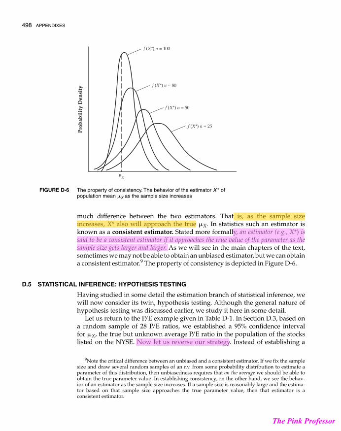
much difference between the two estimators. That is, as the sample sizeincreases, X* also will approach the true . In statistics such an estimator isknown as a consistent estimator. Stated more formally, an estimator (e.g., X*) issaid to be a consistent estimator if it approaches the true value of the parameter as thesample size gets larger and larger. As we will see in the main chapters of the text,sometimes we may not be able to obtain an unbiased estimator, but we can obtaina consistent estimator.9 The property of consistency is depicted in Figure D-6.

D.5 STATISTICAL INFERENCE: HYPOTHESIS TESTING

Having studied in some detail the estimation branch of statistical inference, wewill now consider its twin, hypothesis testing. Although the general nature ofhypothesis testing was discussed earlier, we study it here in some detail.

Let us return to the P/E example given in Table D-1. In Section D.3, based ona random sample of 28 P/E ratios, we established a 95% confidence intervalfor , the true but unknown average P/E ratio in the population of the stockslisted on the NYSE. Now let us reverse our strategy. Instead of establishing a

�X

�X

498 APPENDIXES

f (X*) n = 100

f (X*) n = 80

f (X*) n = 50

f (X*) n = 25

Pro

bab

ilit

y D

ensi

ty

μX

The property of consistency. The behavior of the estimator X * ofpopulation mean X as the sample size increases�

FIGURE D-6

9Note the critical difference between an unbiased and a consistent estimator. If we fix the samplesize and draw several random samples of an r.v. from some probability distribution to estimate aparameter of this distribution, then unbiasedness requires that on the average we should be able toobtain the true parameter value. In establishing consistency, on the other hand, we see the behav-ior of an estimator as the sample size increases. If a sample size is reasonably large and the estima-tor based on that sample size approaches the true parameter value, then that estimator is aconsistent estimator.

guj75845_appD.qxd 4/16/09 12:42 PM Page 498

The Pink Professor

confidence interval, suppose we hypothesize that the true takes a particularnumerical value (e.g., . Our task now is to test this hypothesis.10 Howdo we test this hypothesis—that is, support or refute it?

In the language of hypothesis testing a hypothesis such as is called anull hypothesis and is generally denoted by the symbol H0. Thus, .The null hypothesis is usually tested against an alternative hypothesis, denotedby the symbol H1. The alternative hypothesis can take one of these forms:

H1: 18.5, which is called a one-sided or one-tailed alternative hypothe-sis, or

H1: , also a one-sided or one-tailed alternative hypothesis, or, whichiscalledacomposite,two-sided,ortwo-tailed alternative

hypothesis. That is, the true mean value is either greater than or less than 18.5.11

To test the null hypothesis (against the alternative hypothesis), we use thesample data (e.g., the sample average P/E ratio of 23.25 obtained from the samplein Table D-1) and statistical theory to develop decision rules that will tell uswhether the sample evidence supports the null hypothesis. If the sampleevidence supports the null hypothesis, we do not reject H0, but if it does not, wereject H0. In the latter case we may accept the alternative hypothesis, H1.

How do we develop these decision rules? There are two complementaryapproaches: (1) confidence interval and (2) test of significance. We illustrateeach with the aid of our P/E example. Assume that

(a two-sided hypothesis)

The Confidence Interval Approach to Hypothesis Testing

To test the null hypothesis, suppose we have the sample data given in Table D-1.From these data we computed the sample mean of 23.25. We know from ourdiscussion in Section D.3 that the sample mean is distributed normally withmean and variance . But since the true variance is unknown, we replaceit with the sample variance, in which case we know that the sample meanfollows the t distribution, as shown in Eq. (D.3). Based on the t distribution, weobtain the following 95% confidence interval for:

(D.16) (D.7)

We know that confidence intervals provide a range of values that may includethe true with a certain degree of confidence, such as 95 percent. Therefore, if�X

�19.57 … �X … 26.93

�X2 /n�X

H1:�X Z 18.5

H0:�X = 18.5

H1:�X Z 18.5�X 6 18.5

�X 7

H0: �X = 18.5�X = 18.5

�X = 18.5)�X

APPENDIX D: STATISTICAL INFERENCE: ESTIMATION AND HYPOTHESIS TESTING 499

10A hypothesis is “something considered to be true for the purpose of investigation or argument”(Webster’s), or a “supposition made as a basis for reasoning, or as a starting point for furtherinvestigation from known facts” (Oxford English Dictionary).

11There are various ways of stating the null and alternative hypotheses. For example, we couldhave and .H1: �X 6 13H0:�X Ú 13

guj75845_appD.qxd 4/16/09 12:42 PM Page 499

The Pink Professor

this interval does not include a particular null hypothesized value such as18.5, could we not reject this null hypothesis? Yes, we can, with 95% confidence.

From the preceding discussion it should be clear that the topics of confidenceinterval and hypothesis testing are intimately related. In the language ofhypothesis testing, the 95% confidence interval shown in inequality (D.7) (seeFig. D-2) is called the acceptance region and the area outside the acceptanceregion is called the critical region, or the region of rejection, of the null hypoth-esis. The lower and upper limits of the acceptance region are called criticalvalues. In this language, if the acceptance region includes the value of theparameter under H0, we do not reject the null hypothesis. But if it falls outsidethe acceptance region (i.e., it lies within the rejection region), we reject the nullhypothesis. In our example we reject the null hypothesis that sincethe acceptance region given in Eq. (D.7) does not include the null-hypothesizedvalue. It should be clear now why the boundaries of the acceptance region arecalled critical values, for they are the dividing line between accepting andrejecting a null hypothesis.

Type I and Type II Errors: A Digression

In our P/E example we rejected because our sample evidence ofdoes not seem to be compatible with this hypothesis. Does this mean

that the sample shown in Table D-1 did not come from a normal populationwhose mean value was 18.5? We cannot be absolutely sure, for the confidenceinterval given in inequality (D.7) is 95 and not 100 percent. If that is the case,we would be making an error in rejecting . In this case we aresaid to commit a type I error, that is, the error of rejecting a hypothesis when it istrue. By the same token, suppose , in which case, as inequality (D.7)shows, we would not reject this null hypothesis. But quite possibly the samplein Table D-1 did not come from a normal distribution with a mean value of 21.Thus, we are said to commit a type II error, that is, the error of accepting a falsehypothesis. Schematically,

Reject H0 Do not reject H0

H0 is true Type I error Correct decisionH0 is false Correct decision Type II error

Ideally, we would like to minimize both these errors. But, unfortunately, forany given sample size,12 it is not possible to minimize both errors simultaneously.The classical approach to this problem, embodied in the work of statisticiansNeyman and Pearson, is to assume that a type I error is likely to be more seriousin practice than a type II error. Therefore, we should try to keep the probability

H0:�X = 21

H0:�X = 18.5

X = 23.25H0:�X = 18.5

�X = 18.5

�X =

500 APPENDIXES

12The only way to decrease a type II error without increasing a type I error is to increase the sample size, which may not always be easy.

guj75845_appD.qxd 4/16/09 12:42 PM Page 500

The Pink Professor

of committing a type I error at a fairly low level, such as 0.01 or 0.05, and thentry to minimize a type II error as much as possible.13

In the literature the probability of committing a type I error is designated asand is called the level of significance,14 and the probability of committing a

type II error is designated as . Symbolically,

Type I error prob. (rejecting is true)

Type II error prob. (accepting is false)

The probability of not committing a type II error, that is, rejecting H0 when it isfalse, is , which is called the power of the test.

The standard, or classical, approach to hypothesis testing is to fix at levelssuch as 0.01 or 0.05 and then try to maximize the power of the test; that is, tominimize . How this is actually accomplished is involved, and so we leave thesubject for the references.15 Suffice it to note that, in practice, the classicalapproach simply specifies the value of without worrying too much about .But keep in mind that, in practice, in making a decision there is a trade-offbetween the significance level and the power of the test. That is, for a givensample size, if we try to reduce the probability of a type I error, we ipso factoincrease the probability of a type II error and therefore reduce the power of thetest. Thus, instead of using percent, if we were to use percent, wemay be very confident when we reject , but we may not be so confident whenwe do not reject it.

Since the precedent point is important, let us illustrate. For our P/E ratioexample, in Eq. (D.7) we established a 95% confidence. Let us still assume that

but now fix percent and obtain the 99% confidenceinterval, which is (noting that for 99% CI, the critical t values are (-2.771, 2.771)for 27 d.f.):

(D.17)

This 99% confidence interval is also shown in Fig. D-2. Obviously, this intervalis wider than the 95% confidence interval. Since this interval includes thehypothesized value of 18.5, we do not reject the null hypothesis, whereas inEq. (D.7) we rejected the null hypothesis on the basis of a 95% confidenceinterval. What now? By reducing a type I error from 5 percent to 1 percent, wehave increased the probability of a type II error. That is, in not rejecting the nullhypothesis on the basis of Eq. (D.17), we may be falsely accepting the hypothesis

18.28 … �X … 28.22

� = 1H0:�X = 18.5

H0

� = 1� = 5

��

�

�(1 - �)

H0 ƒ H0= � =

H0 ƒ H0= � =

��

APPENDIX D: STATISTICAL INFERENCE: ESTIMATION AND HYPOTHESIS TESTING 501

13To Bayesian statisticians this procedure sounds rather arbitrary because it does not considercarefully the relative seriousness of the two types of errors. For further discussion of this and relatedpoints, see Robert L. Winkler, Introduction to Bayesian Inference and Decision, Holt, Rinehart andWinston, New York, 1972, Chap. 7.

14 is also known as the size of the (statistical) test.15For a somewhat intuitive discussion of this topic, see Gujarati and Porter, Basic Econometrics,

5th ed., McGraw-Hill, New York, 2009, pp. 833–835. Statistical packages, such as MINITAB, cancalculate the power of a test of size .�

�

guj75845_appD.qxd 4/16/09 12:42 PM Page 501

The Pink Professor

that the true is 18.5. So, always keep in mind the trade-off involved betweentype I and type II errors.

You will recognize that the confidence coefficient discussed earlier issimply 1 minus the probability of committing a type I error. Thus, a 95%confidence coefficient means that we are prepared to accept at most a 5 percentprobability of committing a type I error—we do not want to reject the truehypothesis by more than 5 out of 100 times. In short, a 5% level of significance or a95% level or degree of confidence means the same thing.

Let us consider another example to illustrate further the confidence intervalapproach to hypothesis testing.

Example D.3.

The number of peanuts contained in a jar follows the normal distribution,but we do not know its mean and standard deviation, both of which aremeasured in ounces. Twenty jars were selected randomly and it was foundthat the sample mean was 6.5 ounces and the sample standard deviation was2 ounces. Test the hypothesis that the true mean value is 7.5 ounces againstthe hypothesis that it is different from 7.5. Use .Answer: Letting X denote the number of peanuts in a jar, we are given that

, both parameters being unknown. Since the true variance isunknown, if we use its estimator , it follows that

That is, the t distribution with 19 d.f.From the t distribution table given in Table E-2 in Appendix E, we observe

that for 19 d.f.,

Then from expression (D.6) we obtain

Substituting into this inequality, we obtain

(approx.) (D.18)

as the 99% confidence interval for . Since this interval includes thehypothesized value of 7.5, we do not reject the null hypothesis that the true

.

The null hypothesis in our P/E example was and the alternativehypothesis was that , which is a two-sided, or composite, hypothesis.�X Z 18.5

�X = 18.5

�X = 7.5

�X

5.22 … �X … 7.78

X = 6.5, Sx = 2, and n = 20

PaX - 2.861Sx

220… �X … X + 2.861

Sx

220b = 0.99

P(-2.861 … t … 2.861) = 0.99

t =

X - �X

Sx/2n' t19

Sx2

X ' N(mX, �X2 )

� = 1%

(1 - �)

�X

502 APPENDIXES

guj75845_appD.qxd 4/16/09 12:42 PM Page 502

The Pink Professor

How do we handle one-sided alternative hypotheses such as or? Although the confidence interval approach can be easily adapted to

construct one-sided confidence intervals, in practice it is much easier to use thetest of significance approach to hypothesis testing, which we will now discuss.

The Test of Significance Approach to Hypothesis Testing

The test of significance is an alternative, but complementary and perhapsshorter, approach to hypothesis testing. To see the essential points involved,return to the P/E example and Eq. (D.3). We know that

(D.19) (D.3)

follows the t distribution with d.f. In any concrete application we willknow the values of , and n. The only unknown value is . But if wespecify a value for , as we do under H0, then the right-hand side of Eq. (D.3)is known, and therefore we will have a unique t value. And since we know thatthe t of Eq. (D.3) follows the t distribution with , we simply look up thet table to find out the probability of obtaining such a t value.

Observe that if the difference between and is small (in absolute terms),then, as Eq. (D.3) shows, the value will also be small, where means theabsolute t value. In the event that , t will be zero, in which case we donot reject the null hypothesis. Therefore, as the value increasingly deviates fromzero, we will tend to reject the null hypothesis. As the t table shows, for any givend.f., the probability of obtaining an increasingly higher value becomesprogressively smaller. Thus, as gets larger, we will be more and more inclined toreject the null hypothesis. But how large must be before we can reject the nullhypothesis? The answer, as you would suspect, depends on , the probability ofcommitting a type I error, as well as on the d.f., as we will demonstrate shortly.

This is the general idea behind the test of significance approach to hypothe-sis testing. The key idea here is the test statistic—the t statistic—and its proba-bility distribution under the hypothesized value of . Appropriately, in thepresent instance the test is known as the t test since we use the t distribution.(For details of the t distribution, see Section C.2).

In our P/E example and . Let and, as before. Therefore,

(D.20)

Is the computed t value such that we can reject the null hypothesis? We cannotanswer this question without first specifying what chance we are willing to takeif we reject the null hypothesis when it is true. In other words, to answer thisquestion, we must specify , the probability of committing a type I error.Suppose we fix at 5 percent. Since the alternative hypothesis is two-sided,we want to divide the risk of a type I error equally between the two tails of the

��

t =

23.25 - 18.5

9.49/228= 2.6486

H1:�X Z 18.5H0:�X = 18.5n = 28X = 23.25, Sx = 9.49

�X

�ƒ t ƒ

ƒ t ƒƒ t ƒ

ƒ t ƒX = �X

ƒ t ƒƒ t ƒ�XX

(n - 1)

�X

�XX, Sx

(n - 1)

�t =

X - �X

Sx/1n

�X 7 18.5�X 6 18.5

APPENDIX D: STATISTICAL INFERENCE: ESTIMATION AND HYPOTHESIS TESTING 503

guj75845_appD.qxd 4/16/09 12:42 PM Page 503

The Pink Professor

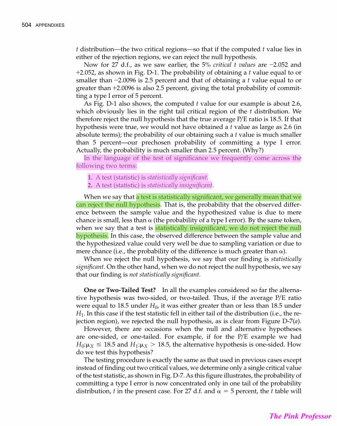
t distribution—the two critical regions—so that if the computed t value lies ineither of the rejection regions, we can reject the null hypothesis.

Now for 27 d.f., as we saw earlier, the 5% critical t values are -2.052 and+2.052, as shown in Fig. D-1. The probability of obtaining a t value equal to orsmaller than -2.0096 is 2.5 percent and that of obtaining a t value equal to orgreater than +2.0096 is also 2.5 percent, giving the total probability of commit-ting a type I error of 5 percent.

As Fig. D-1 also shows, the computed t value for our example is about 2.6,which obviously lies in the right tail critical region of the t distribution. Wetherefore reject the null hypothesis that the true average P/E ratio is 18.5. If thathypothesis were true, we would not have obtained a t value as large as 2.6 (inabsolute terms); the probability of our obtaining such a t value is much smallerthan 5 percent—our prechosen probability of committing a type I error.Actually, the probability is much smaller than 2.5 percent. (Why?)

In the language of the test of significance we frequently come across thefollowing two terms:

1. A test (statistic) is statistically significant.2. A test (statistic) is statistically insignificant.

When we say that a test is statistically significant, we generally mean that wecan reject the null hypothesis. That is, the probability that the observed differ-ence between the sample value and the hypothesized value is due to merechance is small, less than (the probability of a type I error). By the same token,when we say that a test is statistically insignificant, we do not reject the nullhypothesis. In this case, the observed difference between the sample value andthe hypothesized value could very well be due to sampling variation or due tomere chance (i.e., the probability of the difference is much greater than ).

When we reject the null hypothesis, we say that our finding is statisticallysignificant. On the other hand, when we do not reject the null hypothesis, we saythat our finding is not statistically significant.

One or Two-Tailed Test? In all the examples considered so far the alterna-tive hypothesis was two-sided, or two-tailed. Thus, if the average P/E ratiowere equal to 18.5 under H0, it was either greater than or less than 18.5 underH1. In this case if the test statistic fell in either tail of the distribution (i.e., the re-jection region), we rejected the null hypothesis, as is clear from Figure D-7(a).

However, there are occasions when the null and alternative hypothesesare one-sided, or one-tailed. For example, if for the P/E example we had

and , the alternative hypothesis is one-sided. Howdo we test this hypothesis?

The testing procedure is exactly the same as that used in previous cases exceptinstead of finding out two critical values, we determine only a single critical valueof the test statistic, as shown in Fig. D-7. As this figure illustrates, the probability ofcommitting a type I error is now concentrated only in one tail of the probabilitydistribution, t in the present case. For 27 d.f. and percent, the t table will� = 5

H1:�X 7 18.5H0:�X … 18.5

�

�

504 APPENDIXES

guj75845_appD.qxd 4/16/09 12:42 PM Page 504

The Pink Professor

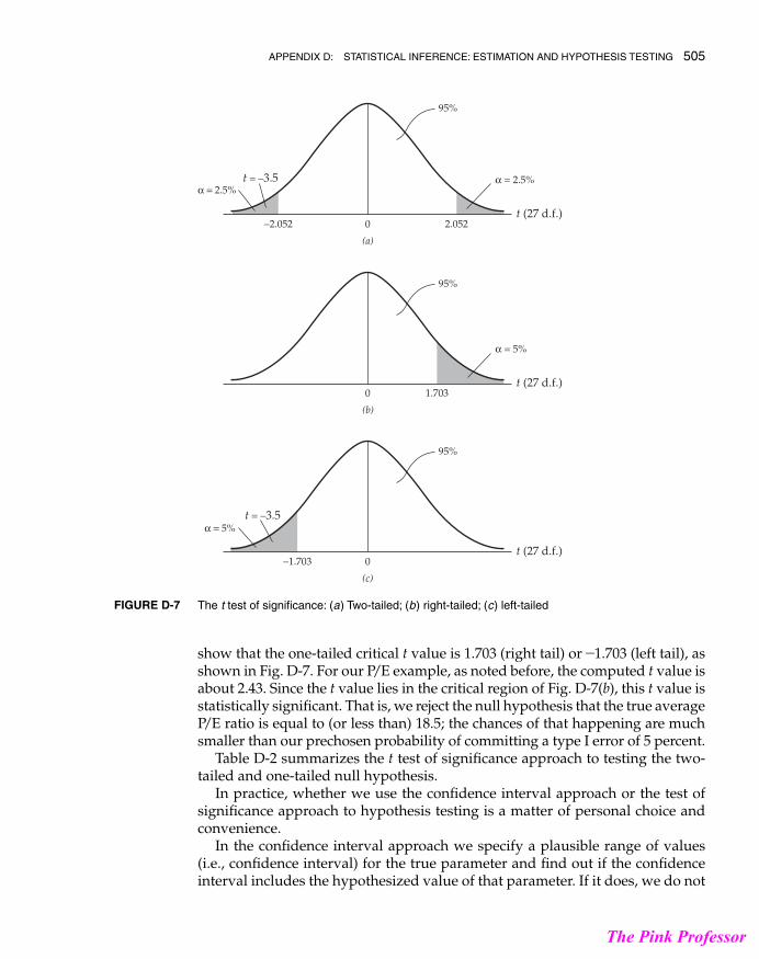
show that the one-tailed critical t value is 1.703 (right tail) or -1.703 (left tail), asshown in Fig. D-7. For our P/E example, as noted before, the computed t value isabout 2.43. Since the t value lies in the critical region of Fig. D-7(b), this t value isstatistically significant. That is, we reject the null hypothesis that the true averageP/E ratio is equal to (or less than) 18.5; the chances of that happening are muchsmaller than our prechosen probability of committing a type I error of 5 percent.

Table D-2 summarizes the t test of significance approach to testing the two-tailed and one-tailed null hypothesis.

In practice, whether we use the confidence interval approach or the test ofsignificance approach to hypothesis testing is a matter of personal choice andconvenience.

In the confidence interval approach we specify a plausible range of values(i.e., confidence interval) for the true parameter and find out if the confidenceinterval includes the hypothesized value of that parameter. If it does, we do not

APPENDIX D: STATISTICAL INFERENCE: ESTIMATION AND HYPOTHESIS TESTING 505

−2.052 0 2.052t (27 d.f.)

α = 2.5%

(a)

α = 2.5%

0 1.703t (27 d.f.)

(b)

α = 5%

0t (27 d.f.)

(c)

−1.703

95%

95%

t = −3.5

α = 5%t = −3.5

95%

The t test of significance: (a) Two-tailed; (b) right-tailed; (c) left-tailedFIGURE D-7

guj75845_appD.qxd 4/16/09 12:42 PM Page 505

The Pink Professor

reject that null hypothesis, but if it lies outside the confidence interval, we canreject the hypothesis.

In the test of significance approach, instead of specifying a range of plausiblevalues for the unknown parameter, we pick a specific value of the parametersuggested by the null hypothesis; compute a test statistic, such as the t statistic;and find its sampling distribution and the probability of obtaining a specificvalue of such a test statistic. If this probability is very low, say, less than or 1 percent, we reject the particular null hypothesis. If this probability is greaterthan the preselected , we do not reject the null hypothesis.

A Word about Accepting or Rejecting a Null Hypothesis In this book wehave used the terminology “reject” or “do not reject” a null hypothesis ratherthan “reject” or “accept” a hypothesis. This is in the same spirit as a jury verdictin a court trial that says whether a defendant is guilty or not guilty rather thanguilty or innocent. The fact that a person is not found guilty does not necessarilymean that he or she is innocent. Similarly, the fact that we do not reject a nullhypothesis does not necessarily mean that the hypothesis is true, becauseanother null hypothesis may be equally compatible with the data. For our P/Eexample, for instance, from Eq. (D.7) it is obvious any value of between 19.57and 26.93 would be an “acceptable” hypothesis.

A Word on Choosing the Level of Significance, �, and the p Value

The Achilles heel of the classical approach to hypothesis testing is its arbitrari-ness in selecting . Although 1, 5, and 10 percent are the commonly used valuesof , there is nothing sacrosanct about these values. As noted earlier, unlesswe examine the consequences of committing both type I and type II errors, wecannot make the appropriate choice of . In practice, it is preferable to find thep value (i.e., the probability value), also known as the exact significance level, ofthe test statistic. This may be defined as the lowest significance level at which a nullhypothesis can be rejected.

�

��

�X

�

� = 5

506 APPENDIXES

A SUMMARY OF THE t TEST

Null hypothesis Alternative hypothesis Critical regionH0 H1 Reject H0 if

Note: denotes the particular value of assumed under the null hypothesis.The first subscript on the t statistic shown in the last column is the level of

significance, and the second subscript is the d.f. These are the critical t values.

�X�0

ƒ t ƒ =

X - �0

Sx/1n 7 t�/2,d.f.�X Z �0�X = �0

t =

X - �0

Sx/1n 6 - t�,d.f.�X 6 �0�X = �0

t =

X - �0

Sx/1n 7 t�,d.f.�X 7 �0�X = �0

TABLE D-2

guj75845_appD.qxd 4/16/09 12:42 PM Page 506

The Pink Professor

To illustrate, in an application involving 20 d.f. a t value of 3.552 wasobtained. The t table given in Appendix E (Table E-2) shows that the p value forthis t is 0.001 (one-tailed) or 0.002 (two-tailed). That is, this t value is statisticallysignificant at the 0.001 (one-tailed) or 0.002 (two-tailed) level.

For our P/E example under the null hypothesis that the true P/E ratio is 18.5,we found that . If the alternative hypothesis is that the true P/E ratio isgreater than 18.5, we find from Table E-1 in Appendix E that is about.01 This is the p value of the t statistic. We say that this t value is statisticallysignificant at the 0.01 or 1 percent level. Put differently, if we were to fix

, at that level we can reject the null hypothesis that the true .Of course, this is a much smaller probability, smaller than the conventional value, such as 5 percent. Therefore, we can reject the null hypothesis much moreemphatically than if we were to choose, say, � = 0.05. As a rule, the smaller thep value, the stronger the evidence against the null hypothesis.

One virtue of quoting the p value is that it avoids the arbitrariness involved infixing atartificial levels, suchas1,5,or10percent. If, forexample, inanapplicationthe p value of a test statistic (such as t) is, say, 0.135, and if you are willing to accept an

percent, this p value is statistically significant (i.e., you reject the nullhypothesis at this level of significance). Nothing is wrong if you want to take achance of being wrong 13.5 percent of the time if you reject the true null hypothesis.

Nowadays several statistical packages routinely compute the p values ofvarious test statistics, and it is recommended that you report these p values.

The 2 and F Tests of Significance

Besides the t test of significance discussed previously, in the main chapters ofthe text we will need tests of significance based on the and the F probabilitydistributions considered in Appendix C. Since the philosophy of testing is thesame, we will simply present here the actual mechanism with a couple ofillustrative examples; we will present further examples in the main text.

The test of significance In Appendix C (see Example C.14) we showedthat if S2 is the sample variance obtained from a random sample of n observa-tions from a normal population with variance , then the quantity

(D.21)

That is, the ratio of the sample variance to population variance multiplied bythe d.f. follows the distribution with d.f. If the d.f. and S2 areknown but is not known, we can establish a confidence interval forthe true but unknown using the distribution. The mechanism is similar tothat for establishing confidence intervals on the basis of the t test.

But if we are given a specific value of under H0, we can directly computethe value from expression (D.21) and test its significance against the critical

values given in Table E-4 in Appendix E. An example follows.�2�2

�2

�2�2(1 - �)%�2(n - 1)�2(n - 1)

(n - 1)aS2

�2b ' �2

(n-1)

�2

X2

�2

X

� = 13.5

�

��X = 18.5� = 0.01

P(t 7 2.43)t = 2.43

APPENDIX D: STATISTICAL INFERENCE: ESTIMATION AND HYPOTHESIS TESTING 507

guj75845_appD.qxd 4/16/09 12:42 PM Page 507

The Pink Professor

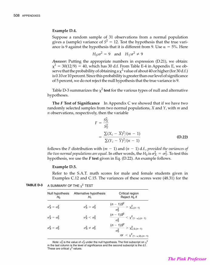
Example D.4.

Suppose a random sample of 31 observations from a normal populationgives a (sample) variance of . Test the hypothesis that the true vari-ance is 9 against the hypothesis that it is different from 9. Use . Here

Answer: Putting the appropriate numbers in expression (D.21), we obtain:which has 30 d.f. From Table E-4 in Appendix E, we ob-

serve that the probability of obtaining a value of about 40 or higher (for 30 d.f.)is 0.10 or 10 percent. Since this probability is greater than our level of significanceof 5 percent, we do not reject the null hypothesis that the true variance is 9.

Table D-3 summarizes the test for the various types of null and alternativehypotheses.

The F Test of Significance In Appendix C we showed that if we have tworandomly selected samples from two normal populations, X and Y, with m andn observations, respectively, then the variable

(D.22)

follows the F distribution with and d.f., provided the variances ofthe two normal populations are equal. In other words, the H0 is . To test thishypothesis, we use the F test given in Eq. (D.22). An example follows.

Example D.5.

Refer to the S.A.T. math scores for male and female students given inExamples C.12 and C.15. The variances of these scores were (48.31) for the

�2X = �2

Y

(n - 1)(m - 1)

=

g (Xi - X)2>(m - 1)

g (Yi - Y)2>(n - 1)

F =

S2X

S2Y

�2

�2�2

= 30(12>9) = 40,

H0:�2= 9 and H1:�2

Z 9

� = 5%S2

= 12

508 APPENDIXES

A SUMMARY OF THE TEST

Null hypothesis Alternative hypothesis Critical regionH0 H1 Reject H0 if

or

Note: is the value of under the null hypothesis. The first subscript on in the last column is the level of significance and the second subscript is the d.f.These are critical values.�2

�2�2X�2

0

6 �2(1-�>2),(n-1)

(n - 1)S2

�20

7 �2�>2,(n-1)�2

X Z �20�2

X = �20

(n - 1)S2

�20

6 �2 (1-�),(n-1)�2

X 6 �20�2

X = �20

(n - 1)S2

�20

7 �2�,(n-1)�2

X 7 �20�2

X = �20

�2TABLE D-3

guj75845_appD.qxd 4/16/09 12:42 PM Page 508

The Pink Professor

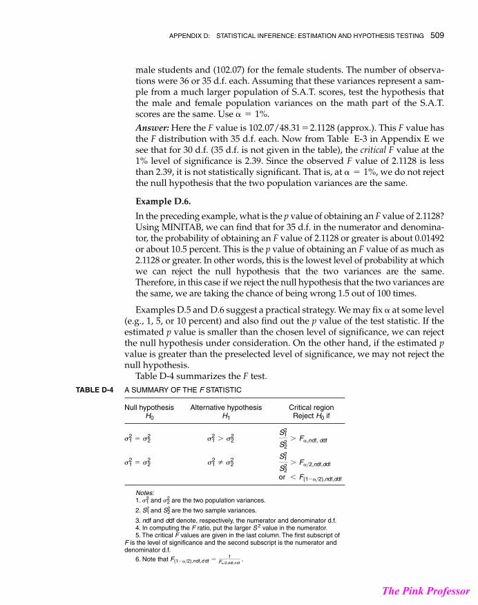
male students and (102.07) for the female students. The number of observa-tions were 36 or 35 d.f. each. Assuming that these variances represent a sam-ple from a much larger population of S.A.T. scores, test the hypothesis thatthe male and female population variances on the math part of the S.A.T.scores are the same. Use .Answer: Here the F value is 102.07/48.31 = 2.1128 (approx.). This F value hasthe F distribution with 35 d.f. each. Now from Table E-3 in Appendix E wesee that for 30 d.f. (35 d.f. is not given in the table), the critical F value at the1% level of significance is 2.39. Since the observed F value of 2.1128 is lessthan 2.39, it is not statistically significant. That is, at , we do not rejectthe null hypothesis that the two population variances are the same.

Example D.6.

In the preceding example, what is the p value of obtaining an F value of 2.1128?Using MINITAB, we can find that for 35 d.f. in the numerator and denomina-tor, the probability of obtaining an F value of 2.1128 or greater is about 0.01492or about 10.5 percent. This is the p value of obtaining an F value of as much as2.1128 or greater. In other words, this is the lowest level of probability at whichwe can reject the null hypothesis that the two variances are the same.Therefore, in this case if we reject the null hypothesis that the two variances arethe same, we are taking the chance of being wrong 1.5 out of 100 times.

Examples D.5 and D.6 suggest a practical strategy. We may fix at some level(e.g., 1, 5, or 10 percent) and also find out the p value of the test statistic. If theestimated p value is smaller than the chosen level of significance, we can rejectthe null hypothesis under consideration. On the other hand, if the estimated pvalue is greater than the preselected level of significance, we may not reject thenull hypothesis.

Table D-4 summarizes the F test.

�

� = 1%

� = 1%

APPENDIX D: STATISTICAL INFERENCE: ESTIMATION AND HYPOTHESIS TESTING 509

A SUMMARY OF THE F STATISTIC

Null hypothesis Alternative hypothesis Critical regionH0 H1 Reject H0 if

or

Notes:1. and are the two population variances.

2. and are the two sample variances.

3. ndf and ddf denote, respectively, the numerator and denominator d.f.4. In computing the F ratio, put the larger S 2 value in the numerator.5. The critical F values are given in the last column. The first subscript of

F is the level of significance and the second subscript is the numerator anddenominator d.f.

6. Note that .F(1-�>2),ndf,d df =1

F�/2,ddf,ndf

S22S2

1

�22�2

1

6 F(1-�>2),ndf,ddf

S21

S22

7 F�>2,ndf,ddf�21 Z �2

2�21 = �2

2

S21

S22

7 F�,ndf, ddf�21 7 �2

2�21 = �2

2

TABLE D-4

guj75845_appD.qxd 4/16/09 12:42 PM Page 509

The Pink Professor

To conclude this appendix, we summarize the steps involved in testing astatistical hypothesis:

Step 1: State the null hypothesis H0 and the alternative hypothesis H1 (e.g.,and for our P/E example).

Step 2: Select the test statistic (e.g., ).Step 3: Determine the probability distribution of the test statistic (e.g.,

.Step 4: Choose the level of significance , that is, the probability of commit-

ting a type I error. (But keep in mind our discussion about the p value.)Step 5: Choose the confidence interval or the test of significance approach.

The Confidence Interval Approach Using the probability distribution ofthe test statistic, establish a % confidence interval. If this interval (i.e.,the acceptance region) includes the null-hypothesized value, do not reject the nullhypothesis. But if this interval does not include it, reject the null hypothesis.

The Test of Significance Approach Alternatively, you can follow thisapproach by obtaining the relevant test statistic (e.g., the t statistic) under thenull hypothesis and find out the p value of obtaining a specified value of the teststatistic from the appropriate probability distribution (e.g., the t, F, or the dis-tribution). If this probability is less than the prechosen value of , you can rejectthe null hypothesis. But if it is greater than , do not reject it. If you do not wantto preselect , just present the p value of the statistic.

Whether you choose the confidence interval or the test of significance ap-proach, always keep in mind that in rejecting or not rejecting a null hypothesis you aretaking a chance of being wrong (or p value) percent of the time.

Further uses of the various tests of significance discussed in this appendixwill be illustrated throughout the rest of this book.

D.6 SUMMARY

Estimating population parameters on the basis of sample information and test-ing hypotheses about them in light of the sample information are the two mainbranches of (classical) statistical inference. In this appendix we examined theessential features of these branches.

KEY TERMS AND CONCEPTS

The key terms and concepts introduced in this appendix are

�

��

��2

100(1 - �)

�X ' N(�X, �2

X>n)

XH1:�X Z 18.5H0:�X = 18.5

510 APPENDIXES

Statistical inferenceParameter estimation

a) point estimationb) interval estimation

Sampling (probability) distribution

Critical t valuesConfidence interval (CI)

a) confidence coefficientb) random interval (lower limit,

upper limit)

guj75845_appD.qxd 4/16/09 12:42 PM Page 510

The Pink Professor

QUESTIONS

D.1. What is the distinction between each of the following pairs of terms?a. Point estimator and interval estimator.b. Null and alternative hypotheses.c. Type I and type II errors.d. Confidence coefficient and level of significance.e. Type II error and power.

D.2. What is the meaning ofa. Statistical inference. e. Critical value of a test.b. Sampling distribution. f. Level of significance.c. Acceptance region. g. The p value.d. Test statistic.

D.3. Explain carefully the meaning ofa. An unbiased estimator. d. A linear estimator.b. A minimum variance estimator. e. Abest linear unbiased estimator (BLUE).c. A best, or efficient, estimator.

D.4. State whether the following statements are true, false, or uncertain. Justify youranswers.a. An estimator of a parameter is a random variable, but the parameter is non-

random, or fixed.b. An unbiased estimator of a parameter, say, , means that it will always be

equal to .c. An estimator can be a minimum variance estimator without being unbiased.d. An efficient estimator means an estimator with minimum variance.e. An estimator can be BLUE only if its sampling distribution is normal.f. An acceptance region and a confidence interval for any given problem

means the same thing.

�X

�X

APPENDIX D: STATISTICAL INFERENCE: ESTIMATION AND HYPOTHESIS TESTING 511

Level of significanceProbability of committing a type I errorProperties of estimators

a) linearity (linear estimator)b) unbiasedness (unbiased

estimator)c) minimum variance (minimum-

variance estimator)d) efficiency (efficient estimator)e) best linear unbiased estimator

(BLUE)f) consistency (consistent

estimator)Hypothesis testing

a) null hypothesisb) alternative hypothesisc) one-sided; one-tailed

hypothesis

d) two-sided; two-tailed;composite hypothesis

Confidence interval (approach tohypothesis testing)a) acceptance regionb) critical region; region of

rejectionc) critical values

Type I error ( ); level of significance;confidence coefficient

Type II error ( )power of the test

Tests of significance (approach tohypothesis testing)a) Test statistic; t statistic; t testb) testc) F test

The p value

�2

(1 - �)�

(1 - �)�

guj75845_appD.qxd 4/16/09 12:42 PM Page 511

The Pink Professor

g. Atype I error occurs when we reject the null hypothesis even though it is false.h. A type II error occurs when we reject the null hypothesis even though it may

be true.i. As the degrees of freedom (d.f.) increase indefinitely, the t distribution

approaches the normal distribution.j. The central limit theorem states that the sample mean is always distributed

normally.k. The terms level of significance and p value mean the same thing.

D.5. Explain carefully the difference between the confidence interval and test ofsignificance approaches to hypothesis testing.

D.6. Suppose in an example with 40 d.f. that you obtained a t value of 1.35. Since itsp value is somewhere between a 5 and 10 percent level of significance (one-tailed), it is not statistically very significant. Do you agree with this statement?Why or why not?

PROBLEMS

D.7. Find the critical Z values in the following cases:a. (two-tailed test) c. (two-tailed test)b. (one-tailed test) d. (one-tailed test)

D.8. Find the critical t values in the following cases:a. n = 4, (two-tailed test) d. n = 14, (one-tailed test)b. n = 4, (one-tailed test) e. n = 60, (two-tailed test)c. n = 14, (two-tailed test) f. n = 200, (two-tailed test)

D.9. Assume that the per capita income of residents in a country is normally dis-tributed with mean and variance ($ squared).a. What is the probability that the per capita income lies between $800 and

$1200?b. What is the probability that it exceeds $1200?c. What is the probability that it is less than $800?d. Is it true that the probability of per capita income exceeding $5000 is

practically zero?D.10. Continuing with problem D.9, based on a random sample of 1000 members,

suppose that you find the sample mean income, , to be $900.a. Given that , what is the probability of obtaining such a sample

mean value?b. Based on the sample mean, establish a 95% confidence interval for and

find out if this confidence interval includes . If it does not, whatconclusions would you draw?

c. Using the test of significance approach, decide whether you want to acceptor reject the hypothesis that . Which test did you use and why?

D.11. The number of peanuts contained in a jar follows the normal distribution withmean and variance . Quality control inspections over several periodsshow that 5 percent of the jars contain less than 6.5 ounces of peanuts and10 percent contain more than 6.8 ounces.a. Find and .b. What percentage of bottles contain more than 7 ounces?

D.12. The following random sample was obtained from a normal population withmean and variance = 2.

8, 9, 6, 13, 11, 8, 12, 5, 4, 14

�

�2�

�2�

� = $1000

� = $1000�

� = $1000X

�2= 10,000� = $1000

� = 0.05� = 0.01� = 0.05� = 0.05� = 0.01� = 0.05

� = 0.02� = 0.05� = 0.01� = 0.05

512 APPENDIXES

guj75845_appD.qxd 4/16/09 12:42 PM Page 512

The Pink Professor

a. Test: against b. Test: against

Note: use .c. What is the p value in part (a) of this problem?

D.13. Based on a random sample of 10 values from a normal population with meanand standard deviation , you calculated that and the sample stan-

dard deviation = 4. Estimate a 95% confidence interval for the populationmean. Which probability distribution did you use? Why?

D.14. You are told that . Based on a sample of 25observations, you found that .a. What is the sampling distribution of ?b. What is the probability of obtaining an or less?c. From your answer in part (b) of this problem, could such a sample value

have come from the preceding population?D.15. Compute the p values in the following cases:

a.b.c. and 20, respectivelyd.Note: If you cannot get an exact answer from the various probability distribu-tion tables, try to obtain them from a program such as MINITAB or Excel.

D.16. In an application involving 30 d.f. you obtained a t statistic of 0.68. Since this tvalue is not statistically significant even at the 10% level of significance, youcan safely accept the relevant hypothesis. Do you agree with this statement?What is the p value of obtaining such a statistic?

D.17. Let . A random sample of three observations was obtainedfrom this population. Consider the following estimators of :

a. Is an unbiased estimator of ? What about ?b. If both estimators are unbiased, which one would you choose? (Hint:

Compare the variances of the two estimators.)D.18. Refer to Problem C.10 in Appendix C. Suppose a random sample of 10 firms

gave a mean profit of $900,000 and a (sample) standard deviation of $100,000.a. Establish a 95% confidence interval for the true mean profit in the industry.b. Which probability distribution did you use? Why?

D.19. Refer to Example C.14 in Appendix C.a. Establish a 95% confidence interval for the true .b. Test the hypothesis that the true variance is 8.2.

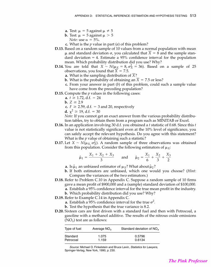
D.20. Sixteen cars are first driven with a standard fuel and then with Petrocoal, agasoline with a methanol additive. The results of the nitrous oxide emissions(NOx) test are as follows:

Type of fuel Average NOx Standard deviation of NOx

Standard 1.075 0.5796Petrocoal 1.159 0.6134

Source: Michael O. Finkelstein and Bruce Levin, Statistics for Lawyers,Springer-Verlag, New York, 1990, p. 230.

�2

N�2�XN�1

N�1 =

X1 + X2 + X3

3 and N�2 =

X1

6+

X2

3+

X3

2

�X

X ' N(�X, �2X)

�2Ú 19, d.f. = 30

F Ú 2.59, d.f. = 3Z Ú 2.9t Ú 1.72, d.f. = 24

X = 7.5X

X = 7.5X ' N(�X = 8, �2

X = 36)

X = 8��

� = 5%� 7 5� = 5� Z 5� = 5

APPENDIX D: STATISTICAL INFERENCE: ESTIMATION AND HYPOTHESIS TESTING 513

guj75845_appD.qxd 4/16/09 12:42 PM Page 513

The Pink Professor

a. How would you test the hypothesis that the two population standarddeviations are the same?

b. Which test did you use? What are the assumptions underlying that test?D.21. Show that the estimator given in Eq. (D.14) is biased. (Hint: Expand Eq. (D.14),

and take the expectation of each term, keeping in mind that the expectedvalue of each Xi is ).

D.22. One-sided confidence interval. Return to the P/E example in this appendix andlook at the two-sided 95% confidence interval given in Eq. (D.7). Suppose youwant to establish a one-sided confidence interval only, either an upper boundor a lower bound. How would you go about establishing such an interval?(Hint: Find the one-tail critical t value.)

�X

514 APPENDIXES

guj75845_appD.qxd 4/16/09 12:42 PM Page 514

The Pink Professor