Astronomy & Astrophysics manuscript no. main c©ESO 2018May 18, 2018

Normal A0–A1 stars with low rotational velocities ?,??

I. Abundance determination and classification

F. Royer1, M. Gebran2, R. Monier3, 4, S. Adelman5, B. Smalley6,O. Pintado7, A. Reiners8, G. Hill9, 10, and A. Gulliver10

1 GEPI/CNRS UMR 8111, Observatoire de Paris – Université Paris Denis Diderot, 5 place Jules Janssen, 92190 Meudon, Francee-mail: frederic.royer@obspm.fr

2 Department of Physics and Astronomy, Notre Dame University-Louaize, PO Box 72, Zouk Mikaël, Lebanon3 LESIA/CNRS UMR 8109, Observatoire de Paris – Université Pierre et Marie Curie – Université Paris Denis Diderot, 5 place Jules

Janssen, 92190 Meudon, France4 Laboratoire Lagrange, Université de Nice Sophia Antipolis, Parc Valrose, 06100 Nice, France5 Department of Physics, The Citadel, 171 Moultrie Street, Charleston, SC 29409, USA6 Astrophysics Group, Keele University, Staffordshire ST5 5BG, UK7 INSUGEO-CONICET, Tucumán, Argentina8 Institut für Astrophysik Göttingen, Physik Fakultät, Friedrich-Hund-Platz 1, 37077 Göttingen, Germany9 18A Stratford St, Auckland, New Zealand

10 Department of Physics and Astronomy, Brandon University, Brandon, MB R7A 6A9, Canada

Received 27 September 2013 / Accepted 23 December 2013

ABSTRACT

Context. The study of rotational velocity distributions for normal stars requires an accurate spectral characterization of the objects inorder to avoid polluting the results with undetected binary or peculiar stars. This piece of information is a key issue in the understand-ing of the link between rotation and the presence of chemical peculiarities.Aims. A sample of 47 low v sin i A0–A1 stars (v sin i < 65km s−1), initially selected as main-sequence normal stars, are investigatedwith high-resolution and high signal-to-noise spectroscopic data. The aim is to detect spectroscopic binaries and chemically peculiarstars, and eventually establish a list of confirmed normal stars.Methods. A detailed abundance analysis and spectral synthesis is performed to derive abundances for 14 chemical species. A hierar-chical classification, taking measurement errors into account, is applied to the abundance space and splits the sample into two differentgroups, identified as the chemically peculiar stars and the normal stars.Results. We show that about one third of the sample is actually composed of spectroscopic binaries (12 double-lined and five single-lined spectroscopic binaries). The hierarchical classification breaks down the remaining sample into 13 chemically peculiar stars (oruncertain) and 17 normal stars.

Key words. stars: early-type – stars: rotation – stars: abundances – stars: chemically peculiar – binaries: spectroscopic

1. Introduction

Observations strongly suggested in the 1960s and 1970s thatslow rotation is a necessary condition for the presence of pe-culiarities in the spectra of A-type stars (Preston 1974, and ref-erences therein). Since then, the equatorial velocity below whichchemically peculiar (hereafter CP) stars are observed is foundto be around 120 km s−1 (Abt & Moyd 1973; Abt & Morrell1995). This observation is supported by theory that links thechemical peculiarities to the diffusion mechanism, occurringwhen the He ii convection zone disappears at equatorial veloc-ities lower than 70–120 km s−1 (Michaud 1982). Atomic diffu-sion, under the competitive action of gravitational settling andradiative accelerations, alters the chemical abundances in stellaratmospheres, when mixing motions are weak. In theory, slow ro-tation should be a sufficient condition for the CP phenomenon to

? Based on observations made at Observatoire de Haute-Provence(CNRS), France?? Tables 1, 2, 4 and 5 are available online only, as well as the appen-dices

appear and Michaud (1980) wondered why a slowly rotating starwould be non-peculiar.

The observational evidence that slow rotation is a sufficientcondition for the presence of chemical peculiarities is not asstraightforward. Whereas the dichotomy between normal and CPstars according to rotation rate is rather clear and unanimous inthe literature for mid to late A-type stars (Abt & Moyd 1973;Abt & Morrell 1995; Royer et al. 2007), this is not the case forearly A-type stars, from A0 to A3.

For Abt & Morrell (1995, hereafter AM), the bimodal shapeof the equatorial velocity distribution can be explained by thedifferent rotation rate of normal stars (fast) compared to peculiarand binary stars (slow). They conclude that the observed over-lap between both distribution modes for A0–A1 stars is due tothe inability to detect marginal CP stars or to evolutionary ef-fects: rotation alone could thus explain the normal or peculiarappearance of an A star’s spectrum (Abt 2000; Adelman 2004).However, authors focusing on the rotational velocities of normalstars confirm the excess of slow rotators for normal A0–A1 stars(Dworetsky 1974; Ramella et al. 1989; Royer et al. 2007), when

Article number, page 1 of 21

arX

iv:1

401.

2372

v1 [

astr

o-ph

.SR

] 1

0 Ja

n 20

14

A&A proofs: manuscript no. main

removing known CP and binary stars. This excess of slow ro-tators is moreover observed at higher masses (Zorec & Royer2012).

The nature of these objects remains unclear. There is nodoubt that a fraction of them is composed of so far unidentifiedspectroscopic binaries and/or CP stars; just how many genuinenormal stars are slow rotators seems very much open again. Areslowly rotating normal A stars young objects that will becomeAp stars and do not show chemical peculiarity yet, as suggestedby Abt (2009)? Since the spectroscopic measurement of rota-tional velocity (v sin i) is a projection on the line-of-sight, are lowv sin i normal abundance A stars likely to be fast rotators seen atlow inclination angle, such as Vega (Gulliver et al. 1994; Hillet al. 2010)? To answer these questions, the low v sin i A0–A1normal stars from Royer et al. (2007, hereafter RZG) need to beinvestigated with new high-resolution and high signal-to-noisespectroscopic data. The purpose of this article is to perform adetailed abundance analysis and spectral synthesis to detect po-tential binary or CP stars and provide a list of confirmed normallow v sin i A0–A1 stars. The resulting subsample will be ana-lyzed in greater depth in a following article.

This paper is organized as follows: the sample, its selectionand the spectroscopic observations are described in Sect. 2. Sec-tion 3 deals with the determination of radial velocities and givesa list of suspected binaries. The atmospheric parameters and ro-tational velocities are respectively derived in Sect. 4 and Sect. 5.Section 6 presents the determination of abundance patterns andSect. 7 details the classification based on these chemical abun-dances. The abundance patterns and the rotational velocity distri-bution are discussed in Sect. 8 and the results are summarized inSect. 9. Comments on individual stars are given in Appendix A.

2. Data sample

2.1. Target selection

RZG built a sample of main-sequence A-type stars with homog-enized v sin i using values from AM and Royer et al. (2002a,b).Chemically peculiar stars were removed on the basis of the spec-tral classification and the catalog of Renson et al. (1991). Binarystars were discarded on the basis of HIPPARCOS data (ESA1997) and the catalog of spectroscopic binaries from Pédoussautet al. (1985). For A0–A1 stars, these criteria reduced the size ofthe original sample by about one third.

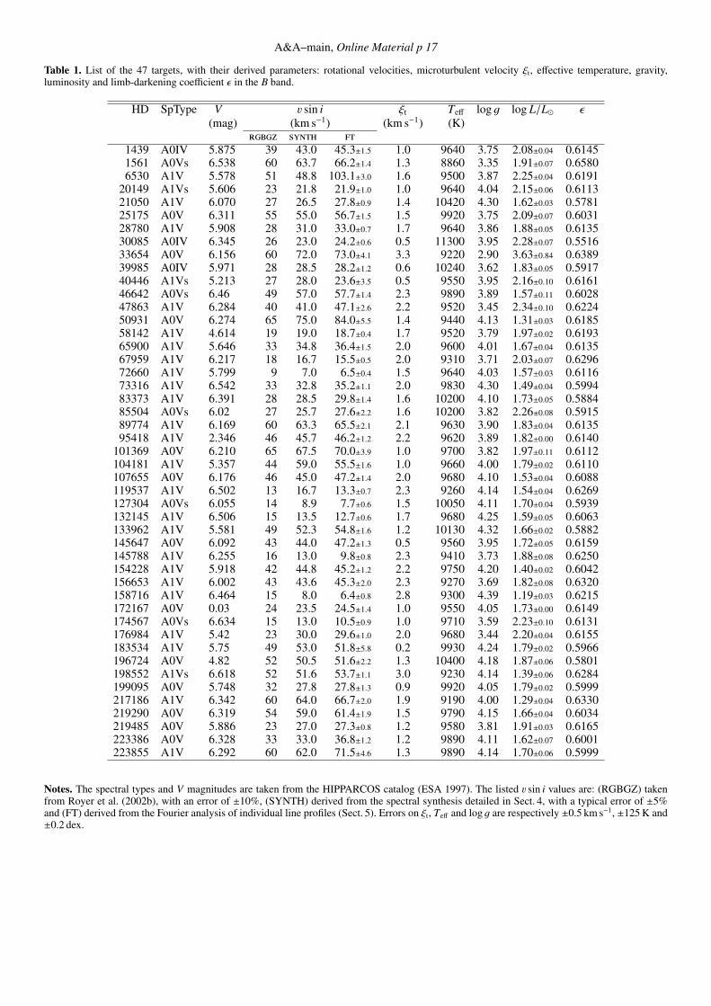
This paper focuses on a subsample of the A0–A1 normalstars, selected on their low v sin i (≤ 65 km s−1), in order to in-vestigate the slow rotator part of the distribution and accuratelycheck whether these stars are normal or harbor signatures ofmultiplicity and/or chemical peculiarity. Using this criterion, 73stars are selected on the whole sky. Among them, 47 can beobserved from Observatoire de Haute-Provence (OHP). Table 1,available online, lists the 47 targets defining our sample, togetherwith their spectral type, V magnitude, v sin i (Royer et al. 2002b)and the different parameters derived in the next sections.

2.2. Spectroscopic observations

Spectra of our targets were collected at OHP and observa-tions were spread over an eight year period. The first two runs(April 2005 and June 2006) used the ÉLODIE spectrograph(R ≈ 42000, Baranne et al. 1996). Then ÉLODIE was de-commissioned in August 2006 and replaced with a more effi-cient instrument offering a higher spectral resolution: SOPHIE(R ≈ 75000, Perruchot et al. 2008). The last part of our program

0 2 4 6V magnitude

1

10

100

# st

ars

0 2 4 6

Fig. 1. Counts in V magnitude bins for northern (δ > −15◦) A0–A1main sequence stars in the HIPPARCOS catalog (gray) and in the v sin isample (hatched).

used SOPHIE, in three different runs: July 2009, February 2011and February 2012. Archival data have also been used: abouthalf the ÉLODIE spectra were taken from the ÉLODIE archive1

(Moultaka et al. 2004) and spectra of Vega were taken from theSOPHIE archive2. Table 2 (available electronically) lists the dif-ferent observations of our targets, indicates the correspondinginstrument, the observation date, the number of co-added spec-tra, the modified Julian date at the center of the exposure(s), thesignal-to-noise ratio (S/N) derived using the DER_SNR algo-rithm (Stoehr et al. 2008) and the measured radial velocity, cor-rected from the barycentric motion (see Sect. 3). The initial ob-servational strategy was derived from the twofold goal of ourprogram: (i) obtain good S/N spectra (≈ 150–200) to perform,using synthetic spectra at low v sin i, a detailed abundance anal-ysis of unblended weak lines, allowing us to identify the nor-mal stars; (ii) focus on these stars and obtain high S/N spec-tra (≈ 400) to analyze the line profiles and search for gravity-darkening signatures.

2.3. Data reduction

For both ÉLODIE and SOPHIE, data are automatically reducedto produce 1D extracted and wavelength calibrated échelle or-ders. When stars are observed several times during one observa-tion night, the corresponding spectra are coadded. Then, for eachreduced spectrum, échelle orders are normalized separately, us-ing a Chebychev polynomial fit with sigma clipping, rejectingpoints above 6-σ or below 1-σ of the continuum. Normalizedorders are merged together, weighted by the blaze function andresampled in a constant wavelength step ∆λ = 0.02Å. Only thespectral intervals outside the wings of Balmer lines and the atmo-spheric telluric bands are finally retained: 4150–4300Å, 4400–4790Å, 4920–5850Å and 6000–6275Å.

2.4. Completeness

Besides selections in v sin i and the absence of spectroscopic pe-culiarities, the aforedescribed sample is magnitude-limited andcensored in declination and spectral type. These censorships canbe applied to the HIPPARCOS catalog (ESA 1997), completedown to V = 7.3 (Perryman et al. 1997), to estimate the com-pleteness of the sample. The selection criteria are the following:

1 http://atlas.obs-hp.fr/elodie2 http://atlas.obs-hp.fr/sophie

Article number, page 2 of 21

F. Royer et al.: Normal A0–A1 stars with low rotational velocities I.

– declination δ higher than −15◦ to reproduce the observabilitybias due to the location of OHP (i.e. 63% of the celestialsphere),

– spectral class containing A0 or A1, and luminosity class ei-ther V, IV/V or IV, to reproduce the selection made in RZG,

– magnitude V brighter than 6.65 .

This selection results in 303 stars from the HIPPARCOS catalog,among them 240 belong to the sample studied by RZG. The starcounts per bin of V-magnitude are compared in Fig. 1. The ratioof these two counts gives a completeness of about 80%.

When limited to normal stars, using the results from RZG,151 stars remain out of the 240. Our 47 targets correspond to thev sin i-truncated subsample out of these 151 stars.

3. Radial velocities

The normalized spectra are cross-correlated with a synthetictemplate extracted from the POLLUX database3 (Palacios et al.2010) corresponding to the parameters Teff = 9500 K, log g =4 and solar metallicity (computed with synspec48, Hubeny &Lanz 1992), to compute the cross-correlation function (hereafterCCF). The radial velocity is derived from the parabolic fit ofthe upper part (10%) of the CCF and the values are given inTable 2. The error on the radial velocity is determined from thecross-correlation function using the formulation given by Zucker(2003) and assuming the parabolic fit of the CCF.

3.1. Combining ÉLODIE and SOPHIE

Fourteen of our targets have spectra collected with both ÉLODIEand SOPHIE. In order to combine the different velocities and de-tect possible variations, the radial velocity offset between bothinstruments has to be retrieved. Boisse et al. (2012) derive a re-lation giving this offset as a function of the B − V color indexfor late-type stars (G to K). The offset ∆E−S ranges from 0 to−0.25 km s−1 for these spectral types.

To constrain this offset for the considered spectral type,publicly available spectra of Vega (HD 172167) are retrievedfrom the ÉLODIE and SOPHIE archives (respectively 16 ob-servations and 10, see Table 2), and radial velocities are de-rived the exact same way. The respective average velocities are:−13.44 ± 0.05 km s−1 and −13.46 ± 0.07 km s−1. The offset forthe considered spectral type is then defined as the difference be-tween these average velocities:

∆E−S(A0) = 0.02 ± 0.09 km s−1. (1)

This offset is not significantly different from zero, and we choosenot to correct the derived radial velocities for our targets.

3.2. Suspected binaries

The suspicion of binarity from the CCF is raised by the variationof the radial velocity, when several observations are available,and/or by an asymmetric shape of individual CCF.

The variation is taken as significant when the ratio of the ex-ternal error over the internal error is E/I & 2 (Abt et al. 1972).The external error is chosen as the standard deviation of the mea-surements for the different available observations, and the inter-nal error is the one estimated using the formulation from Zucker(2003), which increases with the rotational broadening. Table 3

3 http://pollux.graal.univ-montp2.fr

Table 3. List of targets showing a variation in their radial velocity mea-surements, with the number of observations (N), the average barycentricradial velocity 〈RV〉, the external error E and the internal error I.

HD N 〈RV〉 E I(km s−1) (km s−1) (km s−1)

1561 2 −9.2 13.01 0.6420149 5 −11.0 1.33 0.2046642 2 35.0 4.80 0.7372660 4 4.2 0.70 0.03

119537 2 −3.8 82.92 0.46156653 2 3.3 1.32 0.57174567 2 −12.5 2.36 0.46176984 2 −45.7 2.78 0.50196724 2 −20.1 2.59 0.41199095 2 −10.8 20.14 0.49

0.0

0.2

0.4

0.6

0.8 HD 6530

HD 20149

HD 40446

0.0

0.2

0.4

0.6

0.8co

rrel

atio

n co

effic

ient

HD 50931

HD 101369

HD 119537

−80 0 800.0

0.2

0.4

0.6

0.8 HD 145647

−80 0 80velocity shift

HD 183534

−80 0 80(km s−1)

HD 217186

Fig. 2. Cross-correlation functions of suspected binary stars from theirasymmetric profiles. When available, several observations are overplot-ted. The velocity axis takes the barycentric correction into account.

lists the ten stars with E/I > 2. The number of observations fora given star remains small, as a radial velocity follow-up was notintended. These stars are suspected single-lined spectroscopicbinaries (SB1).

The stars that display an asymmetric CCF are shown inFig. 2. For two of them, several observations are available, and avariable radial velocity is noticed. The objects are suspected tobe double-lined spectroscopic binaries (SB2).

Details on them and comparison with literature data can befound in Appendix A.

4. Atmospheric parameters

We use the revised version of the uvbybeta code written by Napi-wotzki et al. (1993) in order to derive effective temperatures(Teff) and surface gravities (log g). The uvbybetanew relies onthe calibration of the Strömgren photometry indices uvbyβ interms of Teff and log g. The photometric data are taken from

Article number, page 3 of 21

A&A proofs: manuscript no. main

1.0 1.5 2.0 2.5log L/LO • HIPPARCOS

1.0

1.5

2.0

2.5lo

g L

/LO •

CA

LIB

39985

46642

217186

1561

6530

2014940446

183534

Fig. 3. Consistency check using the luminosity derived from the Torreset al. (2010) calibration and the HIPPARCOS parallaxes. The dashedline is the one-to-one relation. The outliers are indicated by open sym-bols, together with their HD number.

Hauck & Mermilliod (1998). The derived fundamental param-eters are displayed in Table 1. According to Napiwotzki et al.(1993), errors on effective temperature are of the order of 2%for Teff < 10000 K. The accuracy of surface gravity ranges from≈ 0.1 dex for early A-type stars to ≈ 0.25 dex for hot B stars. Inour study we fix the errors on Teff and log g to be ±125 K and±0.2 dex respectively.

A consistency check on Teff and log g is performed by com-paring the luminosity derived from the radius calibration (Tor-res et al. 2010), and the luminosity derived from HIPPARCOSparallaxes. Torres et al. (2010) give a polynomial expression ofthe stellar radius as a function of Teff , log g and [Fe/H] values.The luminosity is then derived from the Stefan-Boltzmann law.Absolute magnitudes are derived from the HIPPARCOS paral-laxes (van Leeuwen 2007) and from bolometric corrections inthe V-band, interpolated in the tables from Bessell et al. (1998).The adopted bolometric luminosity parameter log L/L�, givenin Table 1, is derived by adopting Mbol

� = 4.75 (Allen 1973).Figure 3 compares the luminosity values. The uncertainty fromthe calibrated luminosity is dominated by the log g uncertainty.In most cases the two agree to within the uncertainties, but afew outliers are present. These eight stars are indicated in Fig. 3and seven out of them are suspected binaries from the previoussection. The new outlier is HD 39985 (see Appendix A). In thisplot, HD 33654 is out of range; the low gravity (log g = 2.9)derived from the photometry indicates a giant star, which is con-firmed by the luminosity derived from the HIPPARCOS data:log L/L� = 3.63±0.84, far brighter than the main-sequence. It ismisclassified as a class V luminosity star.

At this point, the following stars are considered as SB2with atmospheric parameters contaminated by their multiplicity(no abundances are derived): HD 1561, HD 6530, HD 20149,HD 39985, HD 40446, HD 46642, HD 50931, HD 101369,HD 119537, HD 145647, HD 183534, HD 217186. In addition,the following stars are considered as binaries without contami-nation of their atmospheric parameters: HD 72660, HD 156653,

4.04 4.02 4.00 3.98 3.96 3.94log(Teff)

1.0

1.5

2.0

2.5

log

L/L

O •

3.5 MO •

3 MO •

2.5 MO •

2 MO •

Fig. 4. H-R diagram of the sample. Stars are plotted with different sym-bols according to their log g, and the same limits are used to defineregions from the model gravity: triangles for 4.2 ≤ log g (red), dia-monds for 3.95 ≤ log g < 4.2 (orange), squares for 3.65 ≤ log g < 3.95(yellow) and circles for log g < 3.65. Evolutionary tracks from BaSTI(Pietrinferni et al. 2006), for Z = 0.0198, with overshooting, are over-plotted for the indicated stellar masses.

HD 174567, HD 176984, HD 196724. HD 199095. HD 33654is also discarded from the sample as we focus on main-sequencestars.

Figure 4 shows the non-SB2 stars of the sample in the H-Rdiagram. Luminosities are derived from the trigonometric paral-laxes. Evolutionary tracks from BaSTI4 (Pietrinferni et al. 2006)are computed with overshooting and for a solar metallicity ofZ = 0.0198. Considering the end of the main-sequence as its red-dest point, just before the hook of the evolutionary track whenthe overall contraction starts, we chose three limits in log g plot-ted in Fig. 4. The first two limits in log g correspond to aboutone third and two thirds of lifetime on the main sequence for ourmass range, according to BaSTI models. At the end of the mainsequence the gravity given by BaSTI models is about log g = 3.5for our mass range, and the last limit, log g = 3.65, correspondsto about 99% of the lifetime on the main sequence and definesa region that does not overlap with the hook in terms of gravityand position in the H-R diagram.

These fundamental parameters are used to calculate LTEmodel atmospheres using ATLAS9 (Kurucz 1993). The AT-LAS9 code assumes a plane-parallel geometry, a gas in hydro-static and radiative equilibrium, and LTE. As explained in Ge-bran et al. (2008), ATLAS9 model atmospheres are calculatedassuming Grevesse & Sauval (1998) solar abundances and usingthe prescriptions given by Smalley (2004) for convection.

5. Rotational velocities

The v sin i values used for the selection of this sample are takenfrom Royer et al. (2002b) who combine determinations fromFourier analysis with the catalog published by Abt & Morrell(1995). Although these values are statistically corrected from the

4 http://albione.oa-teramo.inaf.it

Article number, page 4 of 21

F. Royer et al.: Normal A0–A1 stars with low rotational velocities I.

shift between both scales, this dataset gives the opportunity toderive new and homogeneous projected rotational velocities.

5.1. Determination of v sin i

The spectral synthesis described in Sect. 6 provides determina-tions of v sin i. The same Fourier analysis as in Royer et al.(2002a,b) is also applied to provide an independent determina-tion of v sin i, from the position of the first zero in the Fouriertransform (hereafter FT) of individual lines.

Díaz et al. (2011) point out the fact that Royer et al. (2002a,b)consider a fixed value of the linear limb-darkening coefficient,ε = 0.6, to derive v sin i, neglecting the variation of this coef-ficient with Teff , log g and wavelength. The expected variationof the limb-darkening coefficient in our sample stars can be es-timated using the values of ε tabulated by Claret (2000). In theJohnson B band, ε varies from 0.64 to 0.56 when the effectivetemperature increases from 9000 to 11000 K.

In order to improve the determination of v sin i, ε is taken intoaccount by comparing the position of the first zero with a theoret-ical rotational profile computed with the linear limb-darkeningcoefficient derived from the atmospheric parameters of the stars,interpolated in the tabulated values given in Claret (2000), forthe B band. The derived value of ε is given in Table 1.

The line candidates for v sin i determination are chosenamong the list of 23 lines given by Royer et al. (2002b), lyingin the spectral range 4215–4577 Å. They are retained using cri-teria based on their shapes in the wavelength domain and in thefrequency domain. Error on the v sin i is taken as the standarddeviation of single line determinations. The results are given inTable 1.

5.2. Rotational velocity scale

Figure 5a compares the v sin i derived using FT profiles in theprevious paragraph and the ones resulting from the spectral syn-thesis (described in Sect. 6), from the same data. In this compar-ison, the suspected SB2 have been discarded. The agreement isvery good and the linear relation between both scales is givenby:

v sin iFT = (1.08 ± 0.01) v sin iSYNTH − 1.8 ± 0.3. (2)

The linear fit is overplotted on the data. The slope of the fit showsthat above ∼ 30 km s−1, v sin i derived from FT are slightly higherthan the result of the spectral synthesis. This is due to the factthat the FT method uses individual line profiles and is thereforemore sensitive to blends than spectral synthesis. As mentionedby Royer et al. (2002b), effects of blends are noticeable on the in-dividual v sin i when compared with the value derived from Mg iitriplet at 4481 Å. Two stars in Fig. 5a (and Table 1) show signifi-cant differences in v sin i: HD 47863 and HD 223855.

Figure 5b compares the new determinations to the homoge-nized values given by Royer et al. (2002b, RGBGZ). These latterdeterminations result from the merging of data from Abt & Mor-rell (1995, AM) and values derived from FT. The different sym-bols in the plot correspond to the combined source: AM only,FT only, or combination of both. The systematic overestimationat low v sin i in the determination from Royer et al. (2002b) re-sults from the lower spectral resolution of ÉLODIE comparedto SOPHIE in this work. A significant shift is noticed with thescaled values from AM, whereas no systematic effect is observedwhen comparing to values derived from FT. The linear relation

0 20 40 60 80v sin i SYNTH (km s−1)

0

20

40

60

80

v s

in i

FT

(km

s−1 )

a)

47863

223855

0 20 40 60 80v sin i RGBGZ (km s−1)

0

20

40

60

80v s

in i

FT

(km

s−1 )

b)

Fig. 5. Comparison of the different v sin i determinations given in Ta-ble 1, excluding SB2 stars. (a) The v sin i derived from the first zeroof the FT is compared to the one derived from the spectral synthesis(SYNTH). The linear fit is shown by the thick solid line. The two starswith the largest differences are labeled. (b) The v sin i derived from thefirst zero of the FT is compared to the homogenized merged catalogfrom Royer et al. (2002b, RGBGZ). The different symbols stand fromthe source of the data in the latter: filled squares were from Abt & Mor-rell (1995, AM), filled circles were derived by RGBGZ using Fourieranalysis, open circles are a combination of both sources. The linear fiton the subsample with data from AM is represented by the thick solidline. In both panels, the one-to-one relation is represented by the dashedline.

between both scales (displayed in Fig. 5b) is given by:

v sin iFT = (1.09 ± 0.03) v sin iRGBGZ + 2.8 ± 1.2. (3)

The scaling relation between AM and the FT results is derivedby Royer et al. (2002b) using spectral types from B8 to F2.This relation could slightly vary with the spectral type, as thecomparison restricted to A0–A1-type stars suggests. The sta-

Article number, page 5 of 21

A&A proofs: manuscript no. main

tistical correction applied by Royer et al. (2002b) is v sin i =1.05 v sin iAM + 7.5 and the resulting values for A0–A1 stars maybe undercorrected.

6. Abundance analysis

For the rotational velocity range in our sample (v sin i ≤65 km s−1), the most appropriate method to derive individualchemical abundances is the use of spectrum synthesis technique.Specifically, we iteratively adjust LTE synthetic spectra to theobserved ones by minimizing the χ2 of the models to the obser-vations using Takeda’s (1995) iterative procedure (see Gebranet al. 2008, for a detailed discussion).

6.1. Spectrum synthesis

Takeda’s procedure is divided in two parts. The first part is amodified version of Kurucz (1992) Width9 code and computesthe opacity data. The second part of the routine computes thesynthetic spectrum and minimizes the dispersion between thenormalized synthetic spectrum and the observed one.

The line list used for spectral synthesis is the one used inGebran et al. (2008, 2010). All transitions between 3000 and7000 Å from Kurucz’s gfall.dat5 line list are selected for the cal-culation of the synthetic spectra. The abundance determinationrelies mainly on unblended transitions for about 14 chemical el-ements (C, O, Mg, Si, Ca, Sc, Ti, Cr, Fe, Ni, Sr, Y, Zr, and Ba).Most of these lines are weak because they are formed deep in theatmosphere. They are well suited to abundance determinations asLTE should prevail in the deeper layers of the atmospheres.

The accuracy of the atomic parameters (wavelengths, lowerexcitation potential, oscillator strength and damping constants)is checked against more accurate and/or more recent laboratorydeterminations, using the VALD6 (Kupka et al. 1999) and theNIST7 databases. The adopted atomic data for each elements arecollected in Table B.1, where for each element, the wavelength,the oscillator strength, and the reference are given.

A byproduct of this procedure is the derivation of the ro-tational (v sin i) and the microturbulent (ξt) velocities. We firstderive the rotational and microturbulent velocities using severalweak and moderately strong unblended Fe ii lines located be-tween 4491.405 Å and 4522.634 Å and the Mg ii triplet around4481 Å by allowing small variations around solar abundances ofMg and Fe as explained in Sect. 3.2.1 of Gebran et al. (2008).The weak iron lines are very sensitive to rotational velocity butnot to microturbulent velocity while the moderately strong Fe iilines are affected mostly by changes of microturbulent velocity.The Mg ii triplet is sensitive to both ξt and v sin i. The derivedrotational and microturbulent velocities are displayed in Table 1.The error on ξt is ±0.5 km s−1 (Gebran et al. 2010). By testingthe effect of the variation of the v sin i on the abundance de-rived from the Mg ii triplet, we are able to determine ∆(v sin i)that causes a variation of the abundance of about the error level(∆[Mg/H] ∼ σMg). On average we find that the rotational ve-locities have a precision estimated as 5% of the nominal v sin iand are in good agreement with those derived using the Fouriertransforms (Sect. 5).

Once the rotational and microturbulent velocities are fixed,we then derive the abundance that minimized the χ2 for each

5 http://kurucz.harvard.edu/LINELISTS/GFALL6 http://www.astro.uu.se/~vald/php/vald.php7 http://physics.nist.gov/PhysRefData/ASD/lines_form.html

transition of a given chemical element. Figure 6 displays the ob-served spectra of six A stars, for different v sin i, with their re-spective best fit synthetic spectra.

6.2. Resulting abundances

The derived abundances are mean values and given in solar scalein Table 4, available online. For a given chemical element X, theabundance [X/H] is equal to the difference between the absoluteabundance in the star log (X/H)? and the abundance in the Sunlog (X/H)� derived from Grevesse & Sauval (1998). As donein Gebran et al. (2008), errors on the elemental abundances areestimated by the standard deviation, assuming a Gaussian distri-bution of the abundances derived from each line. When only oneline is measured, we adopted an average error on abundances de-rived from the results of Gebran et al. (2008, 2010) and Gebran& Monier (2008) for stars with v sin i < 70 km s−1. This error isfound to be ≈ 0.15 dex.

7. Cluster analysis and classification

A quick look on the abundances listed in Table 4 and how thesedata are distributed in the Sr–Sc plane (Fig. 7b) suggests that sev-eral stars present CP characteristics. The size of our sample al-lows the use of statistical tools to disentangle the CP and normalstars and perform this classification in an automatic way, fromthe full abundance data set.

7.1. Classification criteria

In our temperature domain, the expected CP stars are the metal-lic Am stars (CP1) and the magnetic Ap stars (CP2). The classi-cal definition of CP1 stars relies on Ca, Sc, iron-peak elementsand heavy elements (Conti 1970; Preston 1974), and for the CP2stars it is based on Si, Cr, Sr and Eu (Preston 1974). Among the14 species studied in this work, 10 species correspond to theseclassical definitions, i.e Si, Ca, Sc, Cr, Fe, Ni, Sr, Y, Zr and Ba.

7.2. Hierarchical cluster analysis

Hierarchical cluster analysis, applied to chemical abundances byCowley & Bord (2004), is a bottom-up classification which con-sists in grouping data by proximity in a given space, producinga classification tree from single elements to the entire sample. Itidentifies clusters as a function of distance between elements.This method is applied to our data and clusters are searchedfor in the multi-dimensional space defined by the abundancesfrom Table 4. Abundances are normalized so that the variationof a given elemental abundance over the full sample lies in theinterval [0, 1], ensuring that the different elements are equallyweighted. Proximity is based on the Euclidean distance in themulti-dimensional normalized space. In the resulting classifica-tion tree (Fig. 7a), two main groups appear. They are identifiedas CP and normal stars, based on the median [Sr/H] abundance:this element being very discriminant (Fig. 7b), the group show-ing the highest median [Sr/H] abundance is associated with CPstars, and the other one with normal stars.

The construction of the classification tree does not take er-rors into account. In order to test the effect of the errors on theresulting memberships, new abundances are randomly simulatedby adding Gaussian noise to the measured abundances, using therelated standard deviation. Over 5000 simulations, targets are al-located to one group or the other, and the proportion of allocation

Article number, page 6 of 21

F. Royer et al.: Normal A0–A1 stars with low rotational velocities I.

4480 4490 4500 4510 4520wavelength (Å)

1.0

1.3

1.6

1.9

2.2

2.5no

rmal

ized

flux

1.0

1.3

1.6

1.9

2.2

2.5

f)

e)

d)

c)

b)

a)

Fig. 6. Selected observed spectra for six A-type stars with different values of v sin i (in black) shifted in flux by steps of 0.3 for clarity reasons. Inred lines are the respective synthetic spectra in a region rich in Fe ii, Ti ii, and Mg ii lines. The spectra are sorted from top to bottom by decreasingv sin i. The stars are (a) HD 101369, (b) HD 133962, (c) HD 107655, (d) HD 65900, (e) HD 58142 and (f) HD 72660. Spectra are shifted to restwavelengths.

to one group is taken as the final membership probability. Thisdefines a new classification, taking the abundance errors into ac-count.

This multivariate statistical analysis is performed using R8

(R Development Core Team 2011).

7.3. Resulting classification and comparison with literaturedata

Hierarchical cluster analysis is applied to the 14 species and pro-duces the membership flag f14 (1 for CP, 0 for normal) fromthe direct classification, for each star. The simulations taking er-rors into account give the membership probability p14. Respec-tively, f10 and p10 are produced when applying hierarchical clus-ter analysis to the 10 “classical” species. Figure 8 displays thesefour criteria, also listed in Table 5 (available online).

The four criteria give rather consistent results. The distribu-tion of p14 shows slightly more separated and peaked groupsthan p10, as a result of the additional discriminant species. A fewobjects show discrepant classifications: HD 219485 is classifiedas probably normal in Table 5 because the classification basedon p10 points it as a CP star whereas the other criteria indicate itis normal; two objects are classified as uncertain (HD 1439 and

8 R is a language and environment for statistical computing and graph-ics, available at http://www.r-project.org

HD 219290) because the classification based on 10 species andthe one based on 14 species produce contradictory results.

In order to check how separated are the two groups in thechemical abundance space, we perform a principal componentanalysis to display the data in fewer dimensions. Principal com-ponent analysis is a statistical method that expresses a set of vari-ables, possibly correlated, as a set of linearly uncorrelated vari-ables called principal components. The principal components arelinear combinations of the original variables and are defined insuch a way that they have the largest possible variance. We ap-ply this method to our data and derive the first two principalcomponents from the 14-species abundances. The determinedelemental abundances are projected onto these two new axesin Fig. 9, as well as the 14 axes corresponding to the differentspecies. The first principal component (PC1) derived from thedata explains 38.8% of the total variation and the second one(PC2) explains 15.4% of the variance in the 14-species abun-dances. Figure 9 shows that species from titanium to zirconiumhave strong positive loadings on PC1, whereas oxygen and car-bon have strong negative loadings. On the other hand, PC2 hasstrong loadings from magnesium and silicium. The original datafor the 34 stars are expressed in the first two components andoverplotted in Fig. 9. They are represented according to the clas-sification resulting from the cluster analysis. The dichotomy isvery clear along the first principal component, and the objectsidentified as “uncertain” in Table 5 lie between the two groups.

Article number, page 7 of 21

A&A proofs: manuscript no. main

30085

72660

107655

158716

83373

127304

67959

154228

65900

95418

172167

73316

174567

21050

145788

132145

223855

47863

89774

25175

104181

156653

196724

28780

58142

176984

198552

223386

85504

133962

199095

219485

1439

219290

0

1

2

3

4

5

6

stars (HD number)

distance

CP normal

a)

−1.0 −0.5 0.0 0.5 1.0 1.5[Sr/H]

−1.5

−1.0

−0.5

0.0

0.5

[Sc/

H]

b)

Fig. 7. (a) Dendogram plot of the hierarchical tree resulting from thecluster analysis of the 14-species chemical abundances of the samplewithout errors. The x-axis gives the HD numbers of the stars and they-axis represents the Euclidean distance, in the normalized abundancespace, between subgroups. The two main groups are identified by thelabeled boxes. (b) Scandium abundances as a function of strontium. Thetwo main groups identified above are projected with different symbol:filled triangle stand for CP stars, open circles represent normal stars.

Back in 2007, RZG used the release of the General Catalogof Ap and Am stars from Renson et al. (1991) to identify thechemically peculiar stars. This release is now outdated by Ren-son & Manfroid (2009). The 47 targets of our sample are notpresent in the previous version of the catalog, and the classifica-tion results can be compared with the content of the new release.Among these objects, nine are present in the catalog from Ren-son & Manfroid (2009), and are listed in Table 6. For two thirdsof the common stars, both classifications are in agreement.

On the other hand, four stars are classified as peculiar butare absent from the catalog built by Renson & Manfroid (2009):HD 30085, HD 65900, HD 67959, HD 158716. More details canbe found in Appendix A.

8. Discussion

8.1. Abundance patterns

Figure 10 displays the median abundance patterns for the nor-mal and peculiar stars resulting from our classification. Onlyfully agreeing classifications (all four criteria) are used to de-rive the median abundances, i.e. 21 normal stars and 10 CP stars.

0.0 0.2 0.4 0.6 0.8 1.0p10

0.0

0.2

0.4

0.6

0.8

1.0

p14

CP

normal

0.0 0.2 0.4 0.6 0.8 1.0p10

5

10

510# stars

0.0

0.2

0.4

0.6

0.8

1.0

p14

Fig. 8. Membership to the CP group from the four criteria: probabili-ties using 10 and 14 species (respectively p10 and p14), direct classifi-cations using 10 species (filled symbol for CP stars, open symbol fornormal stars), and using 14 species (triangle for CP stars, circle for nor-mal stars). Lower and left panels are the projected distributions of p10and p14 respectively.

−0.2 0.0 0.2 0.4

−0.6

−0.4

−0.2

0.0

0.2

0.4

PC1

PC2

X

N

N

N

CP

N

N

CP

CP

CP

N

CP

N

N

CP

N

CP

CP

N

N

N

CP

N

CP

N

N

N

N

N

N

X

N

N

N

−4 −2 0 2 4 6

−8

−6

−4

−2

0

2

4

6

O

C

Mg

Ca

Sc

Si

Ba

YZr

Sr

CrFe

NiTi

Fig. 9. Observed sample and species projected on the first and secondprincipal components (see text). The CP and normal stars are indicatedby filled triangles and open circles respectively, according to the resultsfrom the cluster analysis. Filled squares represent the two uncertain ob-jects and the open square stands for the probable normal star. The direc-tions of the arrows show the relative loadings of the species on the firstand second principal components.

The dispersions are represented by the 16th and 84th percentiles,which in the Gaussian case correspond to the ±1-σ standard de-viation.

Article number, page 8 of 21

F. Royer et al.: Normal A0–A1 stars with low rotational velocities I.

C O Mg Si Ca Sc Ti Cr Fe Ni Sr Y Zr Ba

−1.0

−0.5

0.0

0.5

1.0

1.5

[X/H

] (de

x)

a)

6

98

8

7 8 6 6 9

6

5

C O Mg Si Ca Sc Ti Cr Fe Ni Sr Y Zr Ba

−1.0

−0.5

0.0

0.5

1.0

1.5

element

[X/H

] (de

x)

b)

Fig. 10. Abundance patterns are displayed as box and whisker plots for (a) the normal stars and (b) the CP stars. Boxes correspond to the 16th and84th percentiles of the abundance distribution for each element, thick horizontal lines represent the median value, and the whiskers span from theminimum to the maximum values. The width of the boxes is proportional to the square root of the number of values. The horizontal dashed linestands for the solar values. In the top panel, median values and 16th and 84th percentiles derived from the comparison stars are plotted on the rightside of the boxes, as filled squares and thick vertical lines. The number of abundance determinations is indicated when five or more abundancesare available, and all individual determinations are displayed when the number is less than five (see Sect. 8.1).

Table 6. Comparison of the classification with the General Catalog ofAp and Am stars (Renson & Manfroid 2009).

HD Renson & Manfroid (2009) This work58142 A0-A2 normal72660 A1- CP83373 ? A1 Si CP85504 A1 Mn normal95418 A0- Ba Y CP

107655 ? A1- CP127304 ? B9 Si CP145788 ? A1 Si normal154228 ? A1 Si CP

Notes. In the classification from Renson & Manfroid (2009), a dashindicates an Am star and no dash indicates an Ap star. The questionmark indicates doubtful cases.

The abundance pattern for the normal stars is comparedwith data from the Pleiades (Gebran & Monier 2008) andfrom the Ursa Major moving group (Monier 2005). We se-lect nine normal A-type stars corresponding to our observedeffective temperature range (Teff > 8900 K): six stars aremembers of the Pleiades (HD 23763, HD 23948, HD 23629,HD 23632, HD 23489, HD 23387) and three belong to Ursa Ma-jor (HD 1404, HD 12471, HD 209515). They are analyzed by thelatter authors using the same method and the code from Takeda

(1995), ensuring a comparison with homogeneous data. Theirmedian abundance pattern and the corresponding percentiles areoverplotted in Fig. 10a. It should be noted that this compari-son sample is small and does not fully cover all the species.The number of available determinations for each species in thecomparison sample is indicated in the plot. The agreement be-tween both patterns is very good but we notice discrepancies forstrontium and the heavier elements. The comparison stars haveon average a larger rotational broadening: seven of them have100 ≤ v sin i ≤ 200 km s−1.

As far as the abundance pattern for the CP stars is concerned,no object shows a significant underabundance in calcium and theCa abundance is very similar between CP and normal stars. Thistendency is possibly due to the fact that previously known CPstars are not part of our sample. We find that carbon and oxygenare underabundant, in agreement with Roby & Lambert (1990).The iron-peak elements and heavy elements are overabundant,compared to the normal stars.

By construction, the v sin i range is limited in our sample. Noclear trend of abundances versus v sin i is detected in our data,neither on the whole dataset nor considering both groups sepa-rately.

Article number, page 9 of 21

A&A proofs: manuscript no. main

0 100 200 300 400rotational velocity (km s−1)

0

5

10

15

20

25

30#

star

s

0 100 200 300 400

Fig. 11. Distributions of rotational velocities: histograms are the ob-served v sin i (hatched histogram corresponds to the cleaned sample);dashed lines stand for the smoothed distribution of projected rotationalvelocities; solid lines are the distributions of equatorial velocities. Thicklines correspond to the newly cleaned sample of 121 stars whereas thinlines represent the full sample of 151 stars.

8.2. Rotational velocity distribution

Sections 3, 4 and 7 show that our sample is still contaminatedby CP stars and binary stars. These new identifications allowthe analysis of the rotational velocity distribution of normal starswith a much cleaner sample. It can be noticed that in our sample,no CP stars were found with v sin i & 45 km s−1. The contamina-tion by binary stars remains larger than by CP stars.

As defined in Sect. 2.4, our sample of 47 stars is the lowv sin i part of a larger sample of 151 normal A0–A1 stars repre-senting an 80%-complete, magnitude-limited volume. The dis-tribution of rotational velocities of normal A0–A1 can be an-alyzed with this larger sample. The gray histogram in Fig. 11represents the distribution of their observed v sin i. By removingthe 30 stars identified as peculiar and/or binaries in the previoussections, a cleaned subsample of 121 stars is selected, and its dis-tribution of v sin i is showed by the hatched histogram (Fig. 11).The smoothed distributions of v sin i is obtained by applying themethod described in Bowman & Azzalini (1997) and ported to R(R Development Core Team 2011), and are shown by the dashedlines in Fig. 11. These distributions are then rectified from theprojection effect to recover the distributions of equatorial veloci-ties, assuming the rotation axes are randomly oriented (see RZGfor details).

The high probability density for slow velocities disappearsfrom the distribution in the cleaned sample, but a significantproportion (about 14%) of the normal stars rotates slowly atv ≤ 100 km s−1. These results considerably reduce the pres-ence of slowly rotating normal A0–A1 stars. The overdensityat v ≤ 50 km s−1 represents 4% of the distribution, i.e. five stars.

In the sample, the normal star with the lowest v sin i isHD 145788 (v sin i = 9.8 km s−1 as measured from the ÉLODIEspectrum). In the rectified distribution, there is no star rotatingmore slowly than v = 20 km s−1.

9. Summary and conclusion

This work provides the spectroscopic study of a sample of 47A0–A1 stars, initially selected from Royer et al. (2002b, 2007)to be main-sequence, low v sin i, normal stars. The analysis of thecross-correlation profiles, and the variation of radial velocitiesallow the identification of suspected spectroscopic binaries. The

normal

normal SB1

SB2

giant CP SB1

CP

uncertain

Fig. 12. Resulting content of the sample of 47 A0–A1 stars.

Table 7. List of HD identifiers for the single normal stars. The oneswritten in boldface are suspected to be doubtful candidates from thecomparison with literature data (see Appendix A).

21050 25175 28780 47863 58142 73316 8550489774 104181 132145 133962 145788 172167 198552

219485 223386 223855

spectral synthesis and the determination of chemical abundancesare used to identify chemically peculiar stars using a hierarchicalclassification. The results reveal that two thirds of the sampleis composed of spectroscopic binaries and chemically peculiarstars, and only 17 stars turn out to be normal, showing no sign ofmultiplicity nor peculiarity. The final composition of the sampleis given by the pie chart in Fig. 12.

In the framework of a nearly complete, magnitude limitedsample of 121 A0–A1-type normal stars, this implies that thedistribution of equatorial velocities, under the assumption of ran-domly oriented rotation axes, is no longer dominated by a largefraction of slowly rotating stars. Only 14% of the A0–A1 nor-mal stars are rotating at v ≤ 100 km s−1, which correspond toabout 16 objects, and 21% are rotating at v ≤ 120 km s−1. This isto be compared with the corresponding proportions in the non-cleaned sample: 31% and 37% respectively (Fig. 11). The dis-tribution is not bimodal as previously claimed by RZG, but theoverlap with the distribution of equatorial velocity of CP starsseems real, contrary to the conclusion of Abt & Morrell (1995)and Abt (2000).

The 17 normal stars, spectroscopically identified in this pa-per, are listed in Table 7. The objects were not extensively mon-itored in terms of radial velocity and spectroscopic binarity maystill remain undetected in this sample. Possibly doubtful can-didates are indicated in Table 7, which could be either spectro-scopic binaries or marginal CP stars (see Appendix A). The 17normal stars will be more deeply investigated in a forthcom-ing paper to check whether signatures of gravity darkening dueto fast rotation seen pole-on are present in the spectra. If rota-tion axes are randomly oriented, the probability to observe a starwith i ≤ 10◦ is about 1.5%, which would produce just two starsamong the 121 normal A0–A1 stars.

Acknowledgements. We are very thankful to the referee for his/her appropriateand constructive suggestions and his/her proposed corrections to improve thepaper. This work has made use of BaSTI web tools (ver. 5.0.1). This researchhas made use of the VizieR catalog access tool, CDS, Strasbourg, France. We aregrateful to S. Ilovaisky for providing calibration data corresponding to SOPHIEobservations of Vega.

Article number, page 10 of 21

F. Royer et al.: Normal A0–A1 stars with low rotational velocities I.

ReferencesAbt, H. A. 2000, ApJ, 544, 933Abt, H. A. 2009, AJ, 138, 28Abt, H. A., Levy, S. G., & Gandett, L. 1972, AJ, 77, 138Abt, H. A. & Morrell, N. I. 1995, ApJS, 99, 135 (AM)Abt, H. A. & Moyd, K. I. 1973, ApJ, 182, 809Adelman, S. J. 1994, MNRAS, 271, 355Adelman, S. J. 2004, in The A-Star Puzzle, IAU Symp. 224, ed. J. Zverko,

J. Žižnovský, S. J. Adelman, & W. W. Weiss, 1Adelman, S. J. & Pintado, O. I. 1997, A&A, 125, 219Adelman, S. J., Yu, K., & Gulliver, A. F. 2011, Astron. Nachr., 332, 153Allen, C. W. 1973, Astrophysical quantities, 3rd edn. (The Athone Press Univer-

sity of London)Altmann, M. & de Boer, K. S. 2000, A&A, 353, 135Aristidi, E., Carbillet, M., Prieur, J.-L., et al. 1997, A&AS, 126, 555Baranne, A., Queloz, D., Mayor, M., et al. 1996, A&AS, 119, 373Bessell, M. S., Castelli, F., & Plez, B. 1998, A&A, 333, 231Biemont, E., Grevesse, N., Hannaford, P., & Lowe, R. M. 1981, ApJ, 248, 867Biermann, L. & Lübeck, K. 1948, Zeitschrift für Astrophysik, 25, 325Boisse, I., Pepe, F., Perrier, C., et al. 2012, A&A, 545, A55Bowman, A. W. & Azzalini, A. 1997, Applied smoothing techniques for data

analysis: the kernel approach with S-plus illustrations, Oxford statistical sci-ence series No. 18 (Clarendon Press, Oxford)

Claret, A. 2000, A&A, 363, 1081Conti, P. S. 1970, PASP, 82, 781Cowley, C. R. & Bord, D. J. 2004, in The A-Star Puzzle, IAU Symp. 224, ed.

J. Zverko, J. Žižnovský, S. J. Adelman, & W. W. Weiss, 265–281Díaz, C. G., González, J. F., Levato, H., & Grosso, M. 2011, A&A, 531, A143Dworetsky, M. M. 1974, ApJS, 28, 101ESA. 1997, The Hipparcos and Tycho Catalogues, ESA-SP 1200Fossati, L., Ryabchikova, T., Bagnulo, S., et al. 2009, A&A, 503, 945Fuhr, J. R., Martin, G. A., & Wiese, W. L. 1988, Journal of Physical and Chem-

ical Reference Data, 17Gebran, M. & Monier, R. 2008, A&A, 483, 567Gebran, M., Monier, R., & Richard, O. 2008, A&A, 479, 189Gebran, M., Vick, M., Monier, R., & Fossati, L. 2010, A&A, 523, A71Gontcharov, G. A. 2006, Astronomy Letters, 32, 759Grenier, S., Burnage, R., Faraggiana, R., et al. 1999, A&AS, 135, 503Grevesse, N. & Sauval, A. J. 1998, Space Sci. Rev., 85, 161Gulliver, A. F., Hill, G., & Adelman, S. J. 1994, ApJ Lett., 429, L81Hauck, B. & Mermilliod, M. 1998, A&AS, 129, 431Hill, G., Gulliver, A. F., & Adelman, S. J. 2010, ApJ, 712, 250Hill, G. M. 1995, A&A, 294, 536Hubeny, I. & Lanz, T. 1992, A&A, 262, 501Kukarkin, B. V., Kholopov, P. N., Artiukhina, N. M., et al. 1981, Nachrichtenblatt

der Vereinigung der Sternfreunde, 0Kupka, F., Piskunov, N., Ryabchikova, T. A., Stempels, H. C., & Weiss, W. W.

1999, A&AS, 138, 119Kurucz, R. L. 1992, Rev. Mexicana Astron. Astrofis., 23, 45Kurucz, R. L. 1993, in Space Stations and Space Platforms - Concepts, Design,

Infrastructure and Uses (Kurucz CD-ROM, Cambridge, Smithsonian Astro-physical Observatory)

Landstreet, J. D. 1998, A&A, 338, 1041Martinet, L. 1970, A&A, 4, 331Michaud, G. 1980, AJ, 85, 589Michaud, G. 1982, ApJ, 258, 349Miles, B. M. & Wiese, W. L. 1969, Atomic Data, 1, 1Monier, R. 2005, A&A, 442, 563Moultaka, J., Ilovaisky, S. A., Prugniel, P., & Soubiran, C. 2004, PASP, 116, 693Napiwotzki, R., Schoenberner, D., & Wenske, V. 1993, A&A, 268, 653Palacios, A., Gebran, M., Josselin, E., et al. 2010, A&A, 516, A13Palmer, D. R., Walker, E. N., Jones, D. H. P., & Wallis, R. E. 1968, Royal Green-

wich Observatory Bulletins, 135, 385Pédoussaut, A., Capdeville, A., Ginestet, N., & Carquillat, J. M. 1985, List of

spectroscopic binaries from the Toulouse general catalogue, Observatoire deToulouse

Perruchot, S., Kohler, D., Bouchy, F., et al. 2008, in Proc. SPIE, Vol. 7014,Ground-based and Airborne Instrumentation for Astronomy II, ed. I. S.McLean & M. M. Casali

Perryman, M. A. C., Lindegren, L., Kovalevsky, J., et al. 1997, A&A, 323, L49Pickering, J. C., Thorne, A. P., & Perez, R. 2002, ApJS, 138, 247Pietrinferni, A., Cassisi, S., Salaris, M., & Castelli, F. 2006, ApJ, 642, 797Preston, G. W. 1974, ARA&A, 12, 257R Development Core Team. 2011, R: A Language and Environment for Statis-

tical Computing, R Foundation for Statistical Computing, Vienna, Austria,ISBN 3-900051-07-0

Ramella, M., Böhm, C., Gerbaldi, M., & Faraggiana, R. 1989, A&A, 209, 233Renson, P., Gerbaldi, M., & Catalano, F. A. 1991, A&AS, 89, 429Renson, P. & Manfroid, J. 2009, A&A, 498, 961

Roby, S. W. & Lambert, D. L. 1990, ApJS, 73, 67Royer, F., Gerbaldi, M., Faraggiana, R., & Gómez, A. E. 2002a, A&A, 381, 105Royer, F., Grenier, S., Baylac, M.-O., Gómez, A. E., & Zorec, J. 2002b, A&A,

393, 897 (RGBGZ)Royer, F., Zorec, J., & Gómez, A. E. 2007, A&A, 463, 671 (RZG)Schröder, C., Hubrig, S., & Schmitt, J. H. M. M. 2008, A&A, 484, 479Schröder, C. & Schmitt, J. H. M. M. 2007, A&A, 475, 677Sigut, T. A. A. & Landstreet, J. D. 1990, MNRAS, 247, 611Smalley, B. 2004, in The A-Star Puzzle, IAU Symp. 224, ed. J. Zverko,

J. Žižnovský, S. J. Adelman, & W. W. Weiss, 131Stoehr, F., White, R., Smith, M., et al. 2008, in ASP Conf. Ser., Vol. 394, As-

tronomical Data Analysis Software and Systems XVII, ed. R. W. Argyle,P. S. Bunclark, & J. R. Lewis, 505

Takeda, Y. 1995, PASJ, 47, 287Torres, G., Andersen, J., & Giménez, A. 2010, A&AR, 18, 67van Leeuwen, F. 2007, A&A, 474, 653Varenne, O. 1999, A&A, 341, 233Zorec, J. & Royer, F. 2012, A&A, 537, A120Zucker, S. 2003, MNRAS, 342, 1291

Article number, page 11 of 21

A&A–main, Online Material p 12

Appendix A: Comments on individual stars

All our targets are part of the sample studied by Dworetsky(1974), and 25 of them are analyzed by Ramella et al. (1989).In their paper, Ramella et al. (1989) derive v sin i from Fourierprofile analysis and flag the stars according to the agreement be-tween the observed profile and a theoretical rotation profile (‘1’when agreeing, ‘0’ when disagreeing, in their Table 3). Stars la-beled as ‘0’ by Ramella et al. are checked out with our data, andthe Fourier profiles are plotted in Fig. A.3.

Gontcharov (2006) published a compilation of radial veloc-ities and our individual measurements are compared with liter-ature data. The 44 stars in common are plotted in Fig. A.1. TheGaussian fit of the histogram of radial velocity differences givesa standard deviation σ = 2 km s−1. Ten stars show differenceslarger than 3σ. They are indicated in Fig. A.1. The three stars ofour sample (HD 40446, HD 119537 and HD 176984), that arenot present in Gontcharov (2006), are already detected as bina-ries in our data.

−40 −20 0 20 40 60 80 100RV Gontcharov (2006) (km s−1)

−40

−20

0

20

40

60

80

100

RV

this

wor

k (km

s−1 )

1561

201492014928780

50931

127304

172167172167172167172167172167172167172167172167172167172167172167172167172167172167172167172167172167172167172167172167172167172167172167172167172167172167172167

174567

183534199095

217186

Fig. A.1. Comparison of radial velocities between individual valuesfrom Table 2 and the compilation from Gontcharov (2006). The errorbars are the internal errors and the dashed line is the one-to-one rela-tion. The outliers are indicated by open symbols, together with theirHD number.

HD 1439 could not be undoubtedly classified as a normal norCP star, the derived memberships based on 10 and 14 elementsgiving contradictory results (Table 5). It moreover lies in the “un-certain” zone in Fig. 9. The derived abundances in oxygen andmagnesium are high enough to make it classified as a normalstar using all 14 elements whereas the remaining pattern (Si, Ca,Sc, Cr, Fe, Sr, Y and Zr) is rather similar to a CP star. Its ra-dial velocity observed 18 months apart does not show significantvariation.

HD 1561 is variable in radial velocity, from our two observa-tions as well as compared with Gontcharov (2006) who gives aradial velocity of −3 km s−1 (Fig. A.1).

HD 6530 is detected as a spectroscopic binary from its CCF(Fig. 2). The large difference in the v sin i measured using thespectral synthesis and the FT (Table 1) is due to the compositespectrum. It has already been observed by Grenier et al. (1999)who derive the radial velocity and their spectrum is also used byRoyer et al. (2002a) to derive the v sin i. The CCF from this spec-trum is overplotted in Fig.A.2 (black solid line) to emphasize thebinary nature of the star.

0.00.20.40.6

coef

ficie

nt

HD 6530

0.00.20.40.6 HD 20149

−150 −100 −50 0 50 100 150velocity shift (km s−1)

0.00.20.40.6

cor

rela

tion

HD 119537

BA A

B

Fig. A.2. Cross-correlation functions for three suspected binary stars.Top panel: the CCF of the observed spectrum is overplotted to the oneobserved by Grenier et al. (1999). Middle panel: the bisector of theCCF is displayed (dotted line) with a velocity scale enhanced by a factor3, for the sake of clarity. Bottom panel: The two components in thecomposite CCF are labeled as ‘A’ and ‘B’.

HD 20149 is flagged as a suspected binary due to the asym-metry of the CCF. The bisector is displayed in Fig.A.2. The staris labeled as variable in radial velocity in Gontcharov (2006),and the published value (−5 km s−1) is also significantly differ-ent from our determinations (Fig. A.1).

HD 21050 is found to have a large projected rotational velocityby Dworetsky (1974) (v sin i = 60 km s−1) but all other determi-nations are very similar to our result (Palmer et al. 1968; Abt &Morrell 1995; Royer et al. 2002b). Moreover, no spectral vari-ation is detected in our high signal-to-noise observations, col-lected three years apart.

HD 25175 is suspected by Ramella et al. (1989) to be a spec-troscopic binary due to the large broadening and the disagree-ment the observed profile and a theoretical rotational profile.Their determination of v sin i, in good agreement with ours,is much higher than the value derived by Dworetsky (1974)(≤ 40 km s−1). Our Fourier profiles are plotted in Fig. A.3a andthe agreement with the rotational profile is very good, suggest-ing that the broadening is dominated by rotation. Also both ourspectra, observed one year apart, do not show any sign of radialvelocity variation.

HD 28780 has a v sin i significantly different from whatRamella et al. (1989) find (41.3 km s−1). The radial velocity is

A&A–main, Online Material p 13

0.0001

0.0010

0.0100

0.1000

1.0000

ampl

itude

a)

b)

c)

d)

0.01 0.10frequency (s km−1)

0.0001

0.0010

0.0100

0.1000

1.0000

ampl

itude

e)

0.01 0.10frequency (s km−1)

f)

0.01 0.10frequency (s km−1)

g)

0.01 0.10frequency (s km−1)

h)

Fig. A.3. Individual line FT (solid lines) and theoretical rotation profile corresponding to the average v sin i (thick dashed line) for the stars flaggedas ‘0’ by Ramella et al. (1989): (a) HD 25175, (b) HD 65900, (c) HD 67959, (d) HD 72660, (e) HD 85504, (f) HD 127304, (g) HD 145788, (h)HD 223386.

moreover significantly different from the value published byGontcharov (2006): −22.6 km s−1 (Fig. A.1). Although no evi-dence of binarity is detected in our single observation, these dif-ferences suggest that this object could be a spectroscopic binary.

HD 30085 is discarded from v sin i measurement by Ramellaet al. (1989) because of asymmetric line profiles. In our classifi-cation, it falls in the CP group and is newly detected as chemi-cally peculiar.

HD 33654 is identified as a giant star from both its surfacegravity and its luminosity (Table 1), which disagrees with its lu-minosity class: A0V. It was previously classified as a B9III star(Palmer et al. 1968). It is indicated as an Ap Si star in Renson &Manfroid (2009).

HD 39985 is an outlier in our luminosity comparison (Fig. 3)and therefore suspected to be a binary star.

HD 40446 is flagged as a spectroscopic binary by Dworetsky(1974). It is part of the sample studied by Royer et al. (2002b)who determined an uncertain v sin i with a high external error(v sin i = 27: ± 5 km s−1) due to a large dispersion in the valuesderived from individual lines. Its binary nature is confirmed bythe shape of its CCF in Fig. 2.

HD 46642 is suspected to be a photometric variable star(Kukarkin et al. 1981). Our radial velocity measurements reveala variation hence this star is suspected to be a binary.

HD 47863 shows a significant difference between our measure-ments of v sin i, using spectral synthesis and Fourier profile. This

object is however used as a reference star in speckle observationsby Aristidi et al. (1997), suggesting that it is a single star.

HD 50931 is detected as a spectroscopic binary from the dis-torted shape of its CCF. The radial velocity from Gontcharov(2006) is moreover very different from our result: 20 km s−1

(Fig. A.1). The large difference in the v sin i measured using thespectral synthesis and the FT (respectively 75 and 84 km s−1 inTable 1) is due to the composite spectrum.

HD 58142 is found to be a hot Am star by Adelman (1994),which disagrees with our classification. This object lies in thetail of the distribution of memberships (Table 5 and Fig. 8) andcould have been wrongly assigned to the “normal” group.

HD 65900 is suspected by Ramella et al. (1989) to be a spec-troscopic binary due to the large broadening and the disagree-ment between the observed profile and a theoretical rotationalprofile. This disagreement is not seen in our data (Fig. A.3b). Inour classification, it falls in the CP group and is newly detectedas chemically peculiar.

HD 67959 is found to disagree with a rotation profile byRamella et al. (1989), but this is very probably due to its lowv sin i and the fact that instrumental broadening is not negligi-ble. In our data (Fig. A.3c), the main lobe of the FT in observedprofiles is well fitted by the theoretical rotation profile. In ourclassification, it falls in the CP group and is newly detected aschemically peculiar.

HD 72660 is a hot Am star (Varenne 1999), which is consis-tent with our classification. Its low v sin i makes the Fourier pro-

A&A–main, Online Material p 14

files dominated by the instrumental profile, both in Ramella et al.(1989) and in Fig. A.3d. It is listed in Table 3 as variable in radialvelocity, but the variation remains very small. Landstreet (1998)detects an asymmetry in the spectral lines that is attributed to adepth-dependent velocity field.

HD 85504 is flagged by Ramella et al. (1989) as showing a pro-file disagreeing with a rotational broadening. In our data how-ever (Fig. A.3e), the agreement with the theoretical rotationalprofile is good. This object is flagged in Renson & Manfroid(2009) as an Ap Mn star, and manganese is not part of our an-alyzed chemical species. In Adelman & Pintado (1997), it onlyappears slightly metal rich compared to other superficially nor-mal stars with similar effective temperature. This object is more-over known as high spacial velocity (Martinet 1970; Altmann &de Boer 2000) which may be a runaway star. It is a suspectedvariable star (Kukarkin et al. 1981).

HD 95418 is an Am star (Adelman et al. 2011; Hill 1995) andour classification agrees with these results.

HD 101369 is suspected to be a spectroscopic binary from theshape of its CCF (Fig. 2).

HD 107655 belongs to the open cluster Coma Ber. Gebranet al. (2008) derived abundances, using the same method, andtheir values are in good agreement with our determinations, withlarger differences for Sc and Sr. The dispersion in the Sc andSr abundances derived by Gebran et al. (2008) is high; they in-clude more lines than in this study, especially lines located in thewings of Balmer lines. When restricting the comparison to linesin common, the agreement is much better (Table A.1).

Table A.1. Comparison of Sc and Sr abundances of HD 107655 withGebran et al. (2008). The mean abundances, relative to the Sun, aregiven, as well as the absolute abundances for each spectral line. Ellipsisdots (...) indicate when a spectral line has not been used.

Element / line this study Gebran et al. (2008)[Sc/H] 0.178 ± 0.066 −0.2 ± 0.114314.083 Å ... 2.554320.732 Å ... 3.024324.996 Å ... 2.814374.457 Å 3.374 3.145657.896 Å 3.243 3.13[Sr/H] 0.197 ± 0.150 −0.23 ± 0.204077.709 Å ... 2.294215.520 Å 3.127 3.08

HD 119537 is detected as a spectroscopic binary by Dworet-sky (1974). The SB2 nature is clearly visible in our CCFs andthey are plotted for both observations in Fig.A.2 together withthe labels of the components (‘A’ being the component with thehighest correlation peak). The radial velocities given in Table 2are the one corresponding to component A and the differencein radial velocity (A−B) is 153.4 km s−1 in the first observation(2006-06-02) and −140.9 km s−1 on the second (2012-02-14).

HD 127304 is suspected by Ramella et al. (1989) to be a SB2.Our derived radial velocity is moreover significantly differentfrom the value published by Gontcharov (2006), −12.6 km s−1

(Fig. A.1).

HD 132145 is suspected by Ramella et al. (1989) to be a spec-troscopic binary. The observed variation in radial velocity in ourdata is not significant taking the instrumental offset between bothspectrographs into account.

HD 133962 is suspected to be a photometric variable star(Kukarkin et al. 1981).

HD 145647 is suspected to be a binary star from the shape ofthe CCF (Fig. 2).

HD 145788 is studied by Fossati et al. (2009) who do not detectclear signatures of chemical peculiarity and believe this object isa normal star whose abundance pattern reflects the compositionof its progenitor cloud. It is flagged by Ramella et al. (1989)as showing a profile disagreeing with a rotational broadening,probably due to the small rotational broadening. In Fig. A.3g,the shape of the main lobes of the observed profiles agree withthe theoretical rotation profile. This star was only observed withÉLODIE and in our classification, it falls in the normal group. Inthe sample, it is the normal star with the smallest v sin i.

HD 156653 is indicated as a spectroscopic binary by Dworet-sky (1974). Our radial velocity measurements show a ratio ofthe external error over the internal error just above the thresholdused to identify variations in Table 3.

HD 158716 is suspected by Ramella et al. (1989) to be a spec-troscopic binary. In our classification, it falls in the CP group andis newly detected as chemically peculiar.

HD 172167 is, strangely enough, an outlier in Fig. A.1, whereGontcharov (2006) gives a radial velocity of −20.6 km s−1. Vegais not known to have a variable radial velocity on such a scale.

HD 174567 is suspected by Ramella et al. (1989) to be a vari-able CP star (strong Si and variable Sr). It is classified as a nor-mal star according to our measurements but we detect a vari-ation in radial velocity, strengthened by the comparison withGontcharov (2006) in Fig. A.1.

HD 176984 is suspected to be a spectroscopic binary from thevariability of its radial velocity (Table 3).

HD 183534 is detected as a spectroscopic binary from theshape of its CCF (Fig. 2) and the difference in radial velocitywith Gontcharov (2006) in Fig. A.1.

HD 196724 is suspected to be a spectroscopic binary from thevariability of its radial velocity (Table 3).

A&A–main, Online Material p 15

HD 199095 is detected as a spectroscopic binary by Dworetsky(1974). Our measurements show a variation in radial velocity,confirmed when comparing with data from Gontcharov (2006)in Fig. A.1.

HD 217186 is considered to be a possible magnetic field can-didate by Schröder et al. (2008) after being associated with aROSAT X-ray source (Schröder & Schmitt 2007) as a bona fidesingle star. This object is however suspected to be a binary fromthe shape of its CCF (Fig. 2). We have only one spectrum for thisobject, but the comparison with Gontcharov (2006), in Fig. A.1,suggests a variation in radial velocity.

HD 219290 is listed as “uncertain” in Table 5 and lies in the“uncertain” zone in Fig. 9. The high abundances in carbon andoxygen produce contradictory classifications when 10 and 14 areused. The remaining pattern (Si, Ca, Sc, Cr, Fe, Ni, Sr and Zr) israther similar to a CP star.

HD 219485 is listed as “probably normal” in Table 5. It ismarginally classified as a CP star based on the 10 “classical” el-ements. The abundances in Ni and Sr are however significantlyhigher than the median values in the normal star pattern dis-played in Fig. 10.

HD 223386 is flagged as disagreeing from a rotation profile byRamella et al. (1989), but the agreement is very good in our data(Fig. A.3h).

HD 223855 is indicated as a spectroscopic binary by Dworet-sky (1974). It shows a significant difference between the mea-surements of v sin i using spectral synthesis and Fourier profiles,and both values are significantly higher than the one derived byDworetsky (1974): 45 km s−1.

Appendix B: Linelist

The analyzed spectral lines are listed in Table B.1, sorted bychemical element and central wavelength, together with theadopted oscillator strength.

A&A–main, Online Material p 16

Table B.1. Atomic data and their reference for the lines used in our abundances determination.

Element λ (Å) log g f Ref. Element λ (Å) log g f Ref. Element λ (Å) log g f Ref.C i 4932.049 −1.658 1 Sc ii 4246.822 0.242 1 Ni i 4470.472 −0.310 3C i 5052.167 −1.303 1 Sc ii 4374.457 −0.418 1 Ni i 4480.561 −1.491 3C i 5380.337 −1.616 1 Sc ii 4670.407 −0.576 1 Ni i 4490.049 −2.108 3C i 5793.120 −2.063 1 Sc ii 5031.021 −0.400 1 Ni i 4490.525 −2.324 3C i 5800.602 −2.337 1 Sc ii 5239.813 −0.765 1 Ni i 4604.982 −0.250 3O i 5330.726 −2.416 1 Sc ii 5526.790 0.020 1 Ni i 4648.646 −0.100 3O i 5330.735 −1.570 1 Sc ii 5657.896 −0.603 1 Ni i 5080.528 0.330 3O i 5330.741 −0.983 1 Ti ii 4163.644 −0.130 4 Ni i 5099.927 −0.100 3O i 6155.961 −1.363 1 Ti ii 4287.873 −1.790 4 Ni i 5476.904 −0.890 1O i 6155.961 −1.363 1 Ti ii 4417.714 −1.190 4 Sr ii 4215.520 −0.169 1O i 6155.971 −1.011 1 Ti ii 4443.801 −0.720 4 Y ii 4883.684 0.070 3O i 6155.989 −1.120 1 Ti ii 4468.492 −0.600 5 Y ii 4900.120 −0.090 3O i 6156.737 −1.487 1 Ti ii 4501.270 −0.770 4 Y ii 5087.416 −0.170 3O i 6156.755 −0.898 1 Cr ii 4592.049 −1.217 5 Y ii 5200.406 −0.570 3O i 6156.778 −0.694 1 Cr ii 4616.629 −1.291 6 Zr ii 4156.240 −0.776 3O i 6158.149 −1.841 1 Cr ii 4634.070 −0.990 3 Zr ii 4161.210 −0.720 3O i 6158.172 −0.995 1 Cr ii 4812.337 −1.995 3 Zr ii 4208.980 −0.460 3O i 6158.187 −0.409 1 Cr ii 5237.329 −1.160 5 Zr ii 4496.960 −0.810 7Mg ii 4427.994 −1.201 1 Cr ii 5308.440 −1.810 5 Ba ii 4554.029 0.163 3Mg ii 4481.126 0.730 2 Cr ii 5313.590 −1.650 5 Ba ii 4934.076 −0.156 8Mg ii 4481.150 −0.570 2 Fe ii 4273.326 −3.258 5 Ba ii 6141.713 −0.810 1Mg ii 4481.325 0.575 2 Fe ii 4296.572 −3.010 5Si ii 5041.024 0.174 1 Fe ii 4416.830 −2.600 5Si ii 5055.984 0.441 1 Fe ii 4491.405 −2.690 5Si ii 5056.317 −0.535 1 Fe ii 4508.288 −2.210 5Si ii 5466.432 −0.190 3 Fe ii 4515.339 −2.490 5Si ii 5688.817 0.106 1 Fe ii 4520.224 −2.600 5Si ii 5978.930 −0.061 1 Fe ii 4522.634 −2.030 5Ca ii 4489.179 −0.726 3 Fe ii 4541.524 −3.050 5Ca ii 4489.179 −2.157 3 Fe ii 4555.890 −2.290 5Ca ii 4489.179 −0.613 3 Fe ii 4582.835 −3.100 5Ca ii 5001.479 −0.517 1 Fe ii 4656.981 −3.630 5Ca ii 5019.971 −0.257 1 Fe ii 4666.758 −3.330 5Ca ii 5021.138 −1.217 1 Fe ii 4923.927 −1.320 5Ca ii 5285.266 −1.153 1 Fe ii 5197.577 −2.100 5Ca ii 5307.224 −0.853 1 Fe ii 5276.002 −1.940 5

Fe ii 5316.615 −1.850 5

References. (1) NIST; (2) Biermann & Lübeck (1948); (3) Kurucz (http://kurucz.harvard.edu/LINELISTS/GFALL); (4) Pickering et al.(2002); (5) Fuhr et al. (1988); (6) Sigut & Landstreet (1990); (7) Biemont et al. (1981); (8) Miles & Wiese (1969).

A&A–main, Online Material p 17

Table 1. List of the 47 targets, with their derived parameters: rotational velocities, microturbulent velocity ξt, effective temperature, gravity,luminosity and limb-darkening coefficient ε in the B band.

HD SpType V v sin i ξt Teff log g log L/L� ε(mag) (km s−1) (km s−1) (K)

rgbgz synth ft

1439 A0IV 5.875 39 43.0 45.3±1.5 1.0 9640 3.75 2.08±0.04 0.61451561 A0Vs 6.538 60 63.7 66.2±1.4 1.3 8860 3.35 1.91±0.07 0.65806530 A1V 5.578 51 48.8 103.1±3.0 1.6 9500 3.87 2.25±0.04 0.6191

20149 A1Vs 5.606 23 21.8 21.9±1.0 1.0 9640 4.04 2.15±0.06 0.611321050 A1V 6.070 27 26.5 27.8±0.9 1.4 10420 4.30 1.62±0.03 0.578125175 A0V 6.311 55 55.0 56.7±1.5 1.5 9920 3.75 2.09±0.07 0.603128780 A1V 5.908 28 31.0 33.0±0.7 1.7 9640 3.86 1.88±0.05 0.613530085 A0IV 6.345 26 23.0 24.2±0.6 0.5 11300 3.95 2.28±0.07 0.551633654 A0V 6.156 60 72.0 73.0±4.1 3.3 9220 2.90 3.63±0.84 0.638939985 A0IV 5.971 28 28.5 28.2±1.2 0.6 10240 3.62 1.83±0.05 0.591740446 A1Vs 5.213 27 28.0 23.6±3.5 0.5 9550 3.95 2.16±0.10 0.616146642 A0Vs 6.46 49 57.0 57.7±1.4 2.3 9890 3.89 1.57±0.11 0.602847863 A1V 6.284 40 41.0 47.1±2.6 2.2 9520 3.45 2.34±0.10 0.622450931 A0V 6.274 65 75.0 84.0±5.5 1.4 9440 4.13 1.31±0.03 0.618558142 A1V 4.614 19 19.0 18.7±0.4 1.7 9520 3.79 1.97±0.02 0.619365900 A1V 5.646 33 34.8 36.4±1.5 2.0 9600 4.01 1.67±0.04 0.613567959 A1V 6.217 18 16.7 15.5±0.5 2.0 9310 3.71 2.03±0.07 0.629672660 A1V 5.799 9 7.0 6.5±0.4 1.5 9640 4.03 1.57±0.03 0.611673316 A1V 6.542 33 32.8 35.2±1.1 2.0 9830 4.30 1.49±0.04 0.599483373 A1V 6.391 28 28.5 29.8±1.4 1.6 10200 4.10 1.73±0.05 0.588485504 A0Vs 6.02 27 25.7 27.6±2.2 1.6 10200 3.82 2.26±0.08 0.591589774 A1V 6.169 60 63.3 65.5±2.1 2.1 9630 3.90 1.83±0.04 0.613595418 A1V 2.346 46 45.7 46.2±1.2 2.2 9620 3.89 1.82±0.00 0.6140

101369 A0V 6.210 65 67.5 70.0±3.9 1.0 9700 3.82 1.97±0.11 0.6112104181 A1V 5.357 44 59.0 55.5±1.6 1.0 9660 4.00 1.79±0.02 0.6110107655 A0V 6.176 46 45.0 47.2±1.4 2.0 9680 4.10 1.53±0.04 0.6088119537 A1V 6.502 13 16.7 13.3±0.7 2.3 9260 4.14 1.54±0.04 0.6269127304 A0Vs 6.055 14 8.9 7.7±0.6 1.5 10050 4.11 1.70±0.04 0.5939132145 A1V 6.506 15 13.5 12.7±0.6 1.7 9680 4.25 1.59±0.05 0.6063133962 A1V 5.581 49 52.3 54.8±1.6 1.2 10130 4.32 1.66±0.02 0.5882145647 A0V 6.092 43 44.0 47.2±1.3 0.5 9560 3.95 1.72±0.05 0.6159145788 A1V 6.255 16 13.0 9.8±0.8 2.3 9410 3.73 1.88±0.08 0.6250154228 A1V 5.918 42 44.8 45.2±1.2 2.2 9750 4.20 1.40±0.02 0.6042156653 A1V 6.002 43 43.6 45.3±2.0 2.3 9270 3.69 1.82±0.08 0.6320158716 A1V 6.464 15 8.0 6.4±0.8 2.8 9300 4.39 1.19±0.03 0.6215172167 A0V 0.03 24 23.5 24.5±1.4 1.0 9550 4.05 1.73±0.00 0.6149174567 A0Vs 6.634 15 13.0 10.5±0.9 1.0 9710 3.59 2.23±0.10 0.6131176984 A1V 5.42 23 30.0 29.6±1.0 2.0 9680 3.44 2.20±0.04 0.6155183534 A1V 5.75 49 53.0 51.8±5.8 0.2 9930 4.24 1.79±0.02 0.5966196724 A0V 4.82 52 50.5 51.6±2.2 1.3 10400 4.18 1.87±0.06 0.5801198552 A1Vs 6.618 52 51.6 53.7±1.1 3.0 9230 4.14 1.39±0.06 0.6284199095 A0V 5.748 32 27.8 27.8±1.3 0.9 9920 4.05 1.79±0.02 0.5999217186 A1V 6.342 60 64.0 66.7±2.0 1.9 9190 4.00 1.29±0.04 0.6330219290 A0V 6.319 54 59.0 61.4±1.9 1.5 9790 4.15 1.66±0.04 0.6034219485 A0V 5.886 23 27.0 27.3±0.8 1.2 9580 3.81 1.91±0.03 0.6165223386 A0V 6.328 33 33.0 36.8±1.2 1.2 9890 4.11 1.62±0.07 0.6001223855 A1V 6.292 60 62.0 71.5±4.6 1.3 9890 4.14 1.70±0.06 0.5999

Notes. The spectral types and V magnitudes are taken from the HIPPARCOS catalog (ESA 1997). The listed v sin i values are: (RGBGZ) takenfrom Royer et al. (2002b), with an error of ±10%, (SYNTH) derived from the spectral synthesis detailed in Sect. 4, with a typical error of ±5%and (FT) derived from the Fourier analysis of individual line profiles (Sect. 5). Errors on ξt, Teff and log g are respectively ±0.5 km s−1, ±125 K and±0.2 dex.

A&A–main, Online Material p 18

Table 2. List of observations and barycentric radial velocity measurements (RV) for the target sample. Asterisks, following the instrument name,indicate the spectra have been retrieved from the corresponding archive. Spectra observed the same night were combined into one spectrum. Thenumber of input spectra, the modified Julian date (MJD) at the center of the exposure(s) and the combined signal-to-noise (S/N) are also given.

HD Instrument Date # MJD S/N RVspectra (km s−1)

1439 SOPHIE 2009-08-05 1 55049.055625 213 −9.57 ± 0.46SOPHIE 2011-02-11 2 55603.765526 326 −10.38 ± 0.48

1561 SOPHIE 2009-08-05 1 55049.042685 210 −18.44 ± 0.88SOPHIE 2011-02-11 3 55603.792789 337 −0.04 ± 0.92

6530 SOPHIE 2009-08-05 3 55049.122963 387 10.71 ± 2.7520149 ELODIE* 2004-01-02 1 53006.871601 106 −9.01 ± 0.16

SOPHIE 2009-08-05 3 55049.086474 399 −12.11 ± 0.16SOPHIE 2011-02-11 2 55603.834201 356 −12.32 ± 0.16SOPHIE 2012-02-13 2 55970.794641 341 −10.70 ± 0.16SOPHIE 2012-02-14 2 55971.764421 370 −10.88 ± 0.16

21050 SOPHIE 2009-08-05 1 55049.104537 226 −1.10 ± 0.23SOPHIE 2011-02-11 2 55603.856759 69 −1.08 ± 0.44SOPHIE 2012-02-13 2 55970.773571 328 −0.89 ± 0.24

25175 SOPHIE 2011-02-11 1 55603.817766 222 31.62 ± 0.76SOPHIE 2012-02-13 3 55970.818221 308 31.33 ± 0.73

28780 SOPHIE 2012-02-13 2 55970.847066 340 −14.19 ± 0.2930085 SOPHIE 2012-02-13 3 55970.874525 316 8.27 ± 0.2033654 SOPHIE 2012-02-13 2 55970.904277 180 −3.12 ± 1.1039985 ELODIE* 1995-12-20 1 50071.994159 138 13.47 ± 0.2440446 ELODIE* 1999-12-20 1 51532.843002 160 47.80 ± 0.2046642 ELODIE* 2003-01-15 1 52654.978756 190 31.62 ± 0.81

SOPHIE 2012-02-14 3 55971.822326 332 38.41 ± 0.7847863 SOPHIE 2012-02-14 3 55971.789437 365 23.80 ± 0.5250931 SOPHIE 2012-02-14 3 55971.859687 345 42.06 ± 1.4658142 ELODIE* 1998-01-28 1 50841.980507 172 26.94 ± 0.12

ELODIE* 2004-01-03 1 53007.964181 300 26.76 ± 0.12ELODIE* 2005-02-02 1 53403.947654 270 26.90 ± 0.12ELODIE* 2005-02-03 1 53404.944216 292 26.66 ± 0.12

65900 ELODIE* 1995-12-21 1 50072.040836 107 43.06 ± 0.3667959 ELODIE 2005-04-21 1 53481.846784 106 23.74 ± 0.0972660 ELODIE* 1997-03-20 1 50527.808905 64 3.22 ± 0.03

ELODIE* 2004-01-03 1 53007.074899 118 4.28 ± 0.06ELODIE* 2004-01-04 1 53009.017029 152 4.68 ± 0.06ELODIE* 2004-04-11 1 53106.829269 192 4.74 ± 0.07

73316 SOPHIE 2012-02-13 3 55970.946798 146 27.68 ± 0.34SOPHIE 2012-02-14 3 55971.894159 335 28.02 ± 0.33

83373 SOPHIE 2012-02-14 4 55971.999699 292 26.58 ± 0.2485504 ELODIE* 1996-04-24 1 50197.825920 114 103.76 ± 0.24

SOPHIE 2012-02-13 2 55971.001111 63 104.03 ± 0.32SOPHIE 2012-02-14 4 55971.960573 289 103.70 ± 0.24

89774 ELODIE 2005-04-22 1 53482.912204 102 13.28 ± 0.94SOPHIE 2012-02-14 3 55971.926975 293 12.18 ± 0.85

95418 ELODIE* 1997-02-20 1 50499.547959 170 −13.52 ± 0.66ELODIE* 2004-03-10 1 53074.002745 232 −13.73 ± 0.50ELODIE* 2005-02-04 1 53405.056783 283 −13.89 ± 0.53SOPHIE 2011-02-11 5 55604.191435 375 −13.67 ± 0.51

101369 ELODIE 2005-04-21 2 53481.910739 182 7.70 ± 1.79104181 ELODIE* 2004-04-26 1 53121.940547 209 −1.29 ± 0.84

SOPHIE 2012-02-14 3 55972.076979 299 −0.34 ± 0.73107655 ELODIE* 2004-04-08 1 53103.058789 243 −2.74 ± 0.59

SOPHIE 2012-02-14 3 55972.034603 338 −3.49 ± 0.54119537 ELODIE 2006-06-02 1 53888.856696 105 54.81 ± 0.08

SOPHIE 2012-02-14 7 55972.175921 254 −62.46 ± 0.07127304 ELODIE 2005-04-21 1 53481.985365 223 −22.30 ± 0.11132145 ELODIE 2005-04-22 2 53482.066887 219 −9.98 ± 0.07

SOPHIE 2012-02-14 4 55972.113021 277 −9.73 ± 0.07133962 ELODIE 2005-04-22 1 53482.131317 201 −12.63 ± 0.73

A&A–main, Online Material p 19

Table 2. continued.

HD Instrument Date # MJD S/N RVspectra (km s−1)

SOPHIE 2011-02-11 2 55604.224086 215 −13.29 ± 0.73SOPHIE 2012-02-14 3 55972.058538 329 −13.11 ± 0.72

145647 ELODIE 2006-05-31 2 53886.908366 107 −15.12 ± 0.85ELODIE 2006-06-03 1 53889.067390 156 −15.75 ± 0.58

145788 ELODIE 2006-06-01 2 53887.968344 128 −13.05 ± 0.05154228 ELODIE* 1999-06-05 1 51334.988236 163 −31.10 ± 0.50

ELODIE* 1999-06-06 1 51335.970245 244 −31.66 ± 0.47156653 ELODIE* 1996-04-26 1 50199.123847 113 2.37 ± 0.47

SOPHIE 2009-08-05 3 55048.835204 294 4.24 ± 0.46158716 ELODIE 2006-06-02 2 53888.924720 117 −25.44 ± 0.03172167 ELODIE* 2004-02-28 1 53063.215076 266 −13.91 ± 0.19

ELODIE* 2004-03-01 1 53065.215871 288 −13.82 ± 0.20ELODIE* 2004-03-27 1 53091.176158 275 −13.99 ± 0.20ELODIE* 2004-03-29 2 53093.148334 357 −13.91 ± 0.19ELODIE* 2004-08-30 2 53247.816155 378 −13.68 ± 0.19ELODIE* 2004-08-31 2 53248.796281 355 −13.62 ± 0.19ELODIE* 2004-09-23 2 53271.772018 317 −13.77 ± 0.19ELODIE* 2004-09-24 2 53272.771336 320 −13.50 ± 0.19ELODIE* 2004-09-25 2 53273.769548 347 −13.60 ± 0.20ELODIE* 2004-11-05 2 53314.738914 296 −13.52 ± 0.19ELODIE* 2004-11-06 1 53315.726548 246 −13.86 ± 0.18ELODIE* 2004-11-07 2 53316.740124 251 −13.49 ± 0.20ELODIE* 2004-11-09 1 53318.732878 152 −14.01 ± 0.20ELODIE* 2005-04-20 2 53480.107426 309 −13.89 ± 0.19ELODIE* 2005-05-24 2 53514.082351 301 −13.79 ± 0.19ELODIE* 2005-05-25 1 53515.036852 254 −13.94 ± 0.20SOPHIE* 2006-09-08 1 53987.400894 109 −14.07 ± 0.21SOPHIE* 2009-09-28 4 55102.762360 1055 −13.81 ± 0.19SOPHIE* 2009-09-29 1 55103.761169 467 −13.81 ± 0.19SOPHIE* 2009-09-30 1 55104.763217 422 −13.72 ± 0.19SOPHIE* 2009-10-06 1 55110.777199 386 −13.69 ± 0.19SOPHIE* 2009-10-07 2 55111.751158 443 −13.76 ± 0.19SOPHIE* 2009-10-08 1 55112.772696 438 −13.68 ± 0.19SOPHIE* 2009-10-09 1 55113.756793 405 −13.66 ± 0.19SOPHIE* 2009-10-10 3 55114.744915 571 −13.71 ± 0.19SOPHIE* 2009-10-11 1 55115.742314 300 −13.83 ± 0.19

174567 ELODIE 2006-05-31 2 53887.000591 119 −14.18 ± 0.05SOPHIE 2009-08-05 3 55048.871358 355 −10.84 ± 0.05

176984 ELODIE 2006-06-02 1 53888.998090 153 −47.68 ± 0.29SOPHIE 2009-08-05 3 55048.903823 402 −43.75 ± 0.24

183534 ELODIE 2006-06-01 1 53887.075317 148 9.88 ± 0.63196724 ELODIE* 2004-11-12 1 53321.779634 301 −21.97 ± 0.64

ELODIE 2006-06-02 1 53888.083812 156 −18.31 ± 0.52198552 SOPHIE 2009-08-05 2 55048.952500 314 5.47 ± 0.69199095 ELODIE* 2005-10-14 1 53657.768627 168 −24.99 ± 0.21

SOPHIE 2009-08-05 3 55048.925880 325 3.49 ± 0.23217186 SOPHIE 2009-08-05 3 55048.980456 287 18.67 ± 1.34219290 SOPHIE 2009-08-05 2 55049.003953 253 −16.88 ± 0.83219485 SOPHIE 2009-08-05 1 55049.016284 239 −4.48 ± 0.21223386 SOPHIE 2009-08-05 1 55049.027685 235 −18.57 ± 0.34223855 SOPHIE 2009-08-05 1 55049.067083 225 3.68 ± 1.05

A&A–main, Online Material p 20

Tabl

e4.

Abu

ndan

ces

fort

he34

mai

n-se

quen

ceta

rget

sno

tide

ntifi

edas

cont

amin

ated

.Elli

psis

dots

(...)

stan

dfo

rabu

ndan

ces

that

coul

dno

tbe

dete

rmin

edfo

rthe

corr

espo

ndin

gob

ject

.

HD

[C/H

][O

/H]

[Mg/

H]

[Si/H

][C

a/H

][S

c/H

][T

i/H]

[Cr/

H]

[Fe/

H]

[Ni/H

][S

r/H

][Y

/H]

[Zr/

H]

[Ba/

H]

1439

...0.

018±

0.01

80.

220±

0.14

00.

231±

0.06

1−

0.23

2±

0.11

8−

0.09

8±

0.12

5−

0.02

3±

0.04

80.

265±

0.13

50.

072±

0.05

0...

0.63

0±

0.15

00.

685±

0.21

50.

575±

0.00

4...

2105

0−

0.36

0±

0.08

00.

023±

0.04

10.

170±

0.19

00.

175±

0.01

0−

0.13

3±

0.13

8−

0.13

0±

0.23

7−

0.16

6±

0.05

60.

278±

0.16

0−

0.07

5±

0.19

0...

−0.

350±

0.15

0...

0.20

0±

0.18

5...

2517

5−

0.36

5±

0.10

5−

0.01

0±

0.03

00.

025±

0.14

50.

180±

0.10

3−

0.11

5±

0.03

50.

119±

0.10

4−

0.15

1±

0.09

20.

118±

0.05

8−

0.16

0±

0.18

10.

021±

0.31

1−

0.05

0±

0.15

00.

046±

0.15

00.

733±

0.07

70.

817±

0.15

028

780−

0.52

8±

0.04

7−

0.23

5±

0.06

5−

0.07

0±

0.19

0−

0.10

5±

0.17

5−

0.00

7±

0.23

4−

0.08

3±

0.06

80.

013±

0.05

80.

063±

0.09

8−

0.05

0±

0.08

80.

280±

0.14

30.

310±

0.15

00.

225±

0.04

50.

670±

0.11

60.

744±

0.06

930

085−

0.51

8±

0.06

1−

0.16

5±

0.01

5−

0.29

5±

0.09

20.

056±

0.03

30.

003±

0.05

3−

0.19

3±

0.17

90.

163±

0.17

10.

816±

0.35

7−

0.06

7±

0.15

5...

1.11

8±

0.15

02.

096±

0.02

42.

062±

0.08

21.

175±

0.03

547

863−

0.18

5±

0.02

50.

112±

0.15

00.

153±

0.12

70.

200±

0.00

00.

310±

0.02

1−

0.05

7±

0.18

7−

0.43

2±

0.20

9−

0.01

4±

0.09

9−

0.27

0±

0.51

9−

0.03

9±

0.04

1−

0.75

8±

0.15

0−

0.12

8±

0.15

00.

466±

0.02

40.

830±

0.15

058

142−

0.45

2±

0.05

6−

0.24

6±

0.05

6−

0.06

5±

0.17

50.

269±

0.22

1−

0.05

7±

0.41

7−

0.46

6±

0.11

8−

0.16

5±

0.08

50.

055±

0.07

8−

0.00

4±

0.12

40.

287±

0.13

60.

410±

0.15

00.

313±

0.10

50.

550±

0.09

70.

912±

0.16

865

900−

0.56

4±

0.37

9−

0.42

5±

0.05

80.

073±

0.10

30.

421±

0.22

30.

063±

0.24

3−

0.29

8±

0.21

6−

0.02

9±

0.09

30.

378±

0.07

60.

247±

0.12

10.

674±

0.09

30.

805±

0.16

00.

837±

0.09

71.

123±

0.16

61.

433±

0.15

067

959−

0.40

3±

0.02

6−

0.27

0±

0.04

70.

025±

0.24

5...

−0.

079±

0.01

5−

0.22

5±

0.16

70.

153±

0.08

80.

238±

0.06

80.

190±

0.07

50.

494±

0.11

50.

786±

0.15

0...

......

7266

0−

0.61

0±

0.08

2−

0.50

6±

0.06

60.

094±

0.12

70.

295±

0.02

50.

053±

0.11

0−

0.24

5±

0.34

40.

459±

0.11

40.

800±

0.30

60.

456±

0.06

10.

696±

0.10

51.

220±

0.15

00.

835±

0.09

21.

018±

0.05

1...

7331

6−

0.30

8±

0.05

60.

054±

0.05

00.

056±

0.14

60.

068±

0.03

40.

036±

0.20

0−

0.37

4±

0.35

2−

0.07

2±

0.10

90.

085±

0.08

2−

0.21

0±

0.13

2...

−0.

434±

0.15

0...

0.43

0±

0.15

0−

0.09

6±

0.08

283

373

...−

0.23

5±

0.00

50.

095±

0.16

50.

407±

0.05

5−

0.06

5±

0.02

50.

073±

0.23

2−

0.16

6±

0.06

70.

464±

0.16

80.

099±

0.17

0...

0.34

1±

0.15

00.

886±

0.15

00.

640±

0.12

01.

110±

0.15

085

504

0.25

1±

0.14

60.

240±

0.07

60.

412±

0.25

20.

867±

0.35

10.

129±

0.11

90.

358±

0.23

4−

0.03

7±

0.08

80.

382±

0.16

70.

033±

0.11

10.

260±

0.27

0−

0.23

8±

0.15

00.

532±

0.17

20.

613±

0.44

8...

8977

4−

0.36

3±

0.02

70.

167±

0.09

60.

030±

0.20

40.

149±

0.11

1−

0.09

7±

0.18

7−

0.26

9±

0.22

8−

0.11

5±

0.06

90.

165±

0.07

3−

0.03

8±

0.14

90.

057±

0.09

4−

0.09

9±

0.15

00.

474±

0.01

30.

919±

0.01

91.

255±

0.38

595

418−

0.51

0±

0.01

0−

0.32

7±

0.02

40.

052±

0.12

80.

438±

0.27

30.

203±

0.19

5−

0.11

5±

0.10

7−

0.01

7±

0.04

10.

318±

0.09

50.

249±

0.11

00.

400±

0.08

10.

839±

0.15

60.

750±

0.11

51.

057±

0.14

3...

1041

81−

0.04

0±

0.15

00.

028±

0.00

70.

090±

0.15

00.

346±

0.31

7−

0.02

0±

0.15

00.

200±

0.15

00.

035±

0.17

5−

0.00

8±

0.10

2−

0.20

7±

0.02

5−

0.06

2±

0.39

9−

0.33

6±

0.15

0...

0.75

0±

0.26

1...

1076

55−

0.75

0±

0.15

0−

0.58

2±

0.15

0−

0.11

7±

0.15

00.

039±

0.07

3...

0.17

8±

0.06

6−

0.03

5±

0.11

60.

559±

0.08

90.

076±

0.05

50.

771±

0.23

00.

197±

0.15

00.

798±

0.14

90.

815±

0.17

60.

715±

0.15

012

7304−

0.66

7±

0.02

9−

0.41

4±

0.05

00.

013±

0.14

70.

605±

0.31

6−

0.23

7±

0.16

1−

0.01

4±

0.15

00.

070±

0.02

70.

547±

0.17

40.

233±

0.06

10.

655±

0.16

60.

780±

0.15

0...

0.80

7±

0.08

1...

1321

45−

0.18

0±

0.08

8−

0.14

5±

0.08

30.

107±

0.18

30.

271±

0.22

1−

0.06

8±

0.04

1−

0.13

0±

0.16

4−

0.07

6±

0.04

80.

123±

0.04

9−

0.09

7±

0.12

6−

0.04

5±

0.17

4−

0.49

0±

0.15

0...

0.25

4±

0.22

4...

1339

62−

0.16

5±

0.03

3−

0.01

1±

0.02

00.

005±

0.20

5−

0.11

5±

0.15

00.

043±

0.03

70.

000±

0.22

00.

009±

0.07

90.

112±

0.06

90.

019±

0.18

50.

422±

0.12

70.

230±

0.15

0...

0.52

0±

0.27

0...

1457

88−

0.31

2±

0.16

50.

048±

0.08

00.

230±

0.14

00.

265±

0.05

5−

0.16

5±

0.05

9−

0.31

0±

0.07

0−

0.14

5±

0.01

50.

142±

0.08

2−

0.13

7±

0.14

90.

120±

0.21

3−

0.43

0±

0.15

00.

034±

0.08

50.

180±

0.15

0...

1542

28−

0.33

3±

0.38

5−

0.24

0±

0.15

00.

060±

0.17

20.

280±

0.03

0−

0.03

7±

0.50

4−

0.38

7±

0.12

8−

0.00

6±

0.06

00.

433±

0.13

40.

191±

0.07

40.

440±

0.17

70.

460±

0.15

0...

0.76

3±

0.21

4...

1566

53−

0.85

0±

0.11

0−

0.29

2±

0.03

0−

0.05

0±

0.28

00.

008±

0.23

0−

0.17

5±

0.55

80.

082±

0.07

2−

0.19

0±

0.05

70.

133±

0.12

10.

006±

0.10

20.

037±

0.20

30.

245±

0.15

0...

...0.

803±

0.16

315

8716−

0.43

7±

0.13

6−

0.42

7±

0.10

10.

055±

0.11

50.

311±

0.00

7−

0.25

1±

0.38

7−

1.11

4±

0.15

00.

192±

0.02

50.

198±

0.01

30.

235±

0.06

00.

350±

0.11

30.

490±

0.15

00.

775±

0.03

50.

755±

0.12

5...

1721

67−

0.21

0±

0.15

4−

0.05

6±

0.11

5−

0.26

6±

0.17

6−

0.31

3±

0.18

4−

0.31

5±

0.54

8−

0.29

1±

0.19

9−

0.22

5±

0.29

7−

0.34

5±

0.14

4−

0.41

0±

0.09

60.

047±

0.21

6−

0.84

5±

0.15

0...

0.16

0±

0.17

0...

1745

67−

0.45

0±

0.15

0−

0.08

5±

0.13

10.

170±

0.25

00.

195±

0.04

50.

026±

0.21

7−

0.21

0±

0.15

0−

0.20

5±

0.05

50.

190±

0.19

0−

0.03

6±

0.08

50.

130±

0.15

0−

0.21

2±

0.15

00.

218±

0.16

20.

525±

0.06

5...

1769

84−

0.13

3±

0.21

0−

0.20

5±

0.09

50.

260±

0.23

00.

140±

0.15

00.

199±

0.22

6−

0.11

0±

0.15

0−

0.11

7±

0.04

30.

263±

0.11

8−

0.27

6±

0.09

00.

140±

0.45

00.

240±

0.15

00.

145±

0.20

50.

043±

0.06

5...

1967

24...

−0.

328±

0.08

70.

080±

0.15

0−

0.03

0±

0.10

0−

0.18

6±

0.01

7−

0.21

4±

0.15

0−

0.31

4±

0.10

00.

340±

0.22

40.

008±

0.07

70.

138±

0.15

00.

198±

0.15

00.

418±

0.17

40.

585±

0.16

7...

1985

52−

0.19

8±

0.08

2−

0.37

2±

0.03

2−

0.12

0±

0.13

90.

095±

0.27

70.

578±

0.39

2−

0.47

0±

0.21

4−

0.28

0±

0.03

50.

039±

0.11

8−

0.06

9±

0.11

00.

425±

0.12

2−

0.12

0±

0.15

00.

150±

0.08

30.

426±

0.09

2...

1990

95−

0.17

7±

0.10

80.

010±

0.07

3−

0.07

0±

0.31

40.

105±

0.16

2−

0.04

3±

0.10

7−

0.18

5±

0.17

60.

193±

0.16

00.

089±

0.11

60.

029±

0.07

80.

330±

0.34

4−

0.04

0±

0.15

0...

0.50

0±

0.04

0...

2192

900.

160±

0.15

0−

0.08

0±

0.05

70.

100±

0.13

00.

106±

0.03

2−

0.16

0±

0.15

1−

0.01

7±

0.04

8−

0.02

5±

0.07

00.

278±

0.10

40.

015±

0.03

80.

640±

0.15

00.

540±

0.15

0...

0.50

3±

0.15

0...

2194

85−

0.22

0±

0.15

0−

0.13

0±

0.02

10.

140±

0.15

00.

242±

0.35

2−

0.18

3±

0.05

0−

0.39

3±

0.11

1−

0.03

5±

0.04

50.

232±

0.24

20.

034±

0.09

9...

0.55

0±

0.15

00.

260±

0.11

30.

500±

0.15

0...

2233

86...

−0.

174±

0.08

10.

126±

0.15

00.

052±

0.12

6...

−0.

623±

0.25

7−

0.31

5±

0.06

50.

130±

0.09

9−

0.22

7±

0.06

1...

−0.

300±

0.15

00.

049±

0.05

1−

0.02

0±

0.15

0...

2238

55−

0.16

3±

0.09

70.

013±

0.09

00.

270±

0.15

00.

323±

0.38

6...

−0.

115±

0.08

5−

0.21

3±

0.04

20.

022±

0.07

9−

0.03

6±

0.22

4...

−0.

730±

0.15

00.

145±

0.10

50.

340±

0.15

0...

A&A–main, Online Material p 21

Table 5. Probabilities to be CP given by the four different criteria. Classification is deduced from the combination of four probabilities.

HD p10 f10 p14 f14 Classification1439 0.827 1 0.342 0 uncertain

21050 0.107 0 0.012 0 normal25175 0.073 0 0.035 0 normal28780 0.287 0 0.348 0 normal30085 0.986 1 0.983 1 CP47863 0.004 0 0.001 0 normal58142 0.423 0 0.400 0 normal65900 0.999 1 0.994 1 CP67959 0.960 1 0.945 1 CP72660 0.999 1 1.000 1 CP73316 0.014 0 0.010 0 normal83373 0.854 1 0.640 1 CP85504 0.428 0 0.085 0 normal89774 0.166 0 0.051 0 normal95418 0.980 1 0.983 1 CP

104181 0.036 0 0.010 0 normal107655 0.884 1 0.940 1 CP127304 0.997 1 0.999 1 CP132145 0.008 0 0.005 0 normal133962 0.393 0 0.229 0 normal145788 0.012 0 0.001 0 normal154228 0.899 1 0.799 1 CP156653 0.244 0 0.411 0 normal158716 0.756 1 0.916 1 CP172167 0.001 0 0.027 0 normal174567 0.076 0 0.042 0 normal176984 0.087 0 0.054 0 normal196724 0.323 0 0.312 0 normal198552 0.111 0 0.199 0 normal199095 0.261 0 0.189 0 normal219290 0.849 1 0.349 0 uncertain219485 0.637 0 0.402 0 probably normal223386 0.014 0 0.028 0 normal223855 0.018 0 0.001 0 normal