ISR develops, applies and teaches advanced methodologies of design and analysis to solve complex, hierarchical,heterogeneous and dynamic problems of engineering technology and systems for industry and government.

ISR is a permanent institute of the University of Maryland, within the Glenn L. Martin Institute of Technol-ogy/A. James Clark School of Engineering. It is a National Science Foundation Engineering Research Center.

Web site http://www.isr.umd.edu

I RINSTITUTE FOR SYSTEMS RESEARCH

MASTER'S THESIS

Comparing Analytical and Discrete-Event Simulation Models of Manufacturing Systems

by Sara HewittAdvisor: Jeffrey Herrmann

MS 2002-3

ii

ABSTRACT

Title of Thesis: COMPARING ANALYTICAL AND DISCRETE-EVENT

SIMULATION MODELS OF MANUFACTURING SYSTEMS

Degree Candidate: Sara T. Hewitt

Degree and Year: Master of Science, 2002

Thesis directed by: Associate Professor Jeffrey W. Herrmann

Models have a variety of uses in manufacturing as they allow exploration of a

system with mitigated risk to the existing system and mitigated financial risk. Both

analytical models and discrete event simulation models can help elucidate system

behavior, but there can be differences in the results of these two types of models. The

objective of this thesis is to examine the differences between results from analytical

models and discrete event simulation models. A series of case studies serve to illustrate

why analytical models and discrete-event simulation models differ. The creation of a

computer tool called a Learning Historian made it possible to efficiently conduct

experiments of discrete-event simulation models.

A flow shop with process drift provides one example of differing analytical and

discrete-event simulation models. Even after eliminating errors due to different

iii

underlying assumptions, there is a difference between the analytical and simulation

model results because of the inherent variability in the simulation model.

A two-stage system that evolves from a push production control to a hybrid

system to a pull production control system illustrates additional sources of differences

between analytical and discrete event simulation models. The results for the two-stage

push model and the hybrid pull-push model from the analytical and simulation models

generally agree. Significant errors arise for the two-stage pull model because there is no

correct analytical model for the two-stage pull model. The results of the push and pull

production control models illustrate the tradeoff between customer cycle time and

inventory level.

iv

© Copyright by Sara Hewitt

2002

v

COMPARING ANALYTICAL AND DISCRETE-EVENT SIMULATION

MODELS OF MANUFACTURING SYSTEMS

by

Sara T. Hewitt

Thesis submitted to the Faculty of the Graduate School of the University of Maryland, College Park in partial fulfillment

of the requirements for the degree of Master of Science

2002

Advisory Committee:

Associate Professor Jeffrey W. Herrmann Professor Gary W. Rubloff Associate Professor Linda C. Schmidt

vi

DEDICATION

To my family

vii

ACKNOWLEDGEMENTS

I would like to thank Dr. Herrmann for his guidance, insight and patience

throughout the process of creating many models. I would like to thank all of my lab-

mates in the CIM lab for making the lab such a good place to work and Anne Rose and

Catherine Plaisant for their advice about the Learning Historian. I would also like to

thank Dan for his help editing and all of my roommates for their interest in my research.

Finally I would like to thank my parents for all of their support.

viii

CONTENTS

LIST OF FIGURES X

LIST OF TABLES XII

1 INTRODUCTION 1

2 BACKGROUND 4

2.1 INTRODUCTION 4 2.2 ANALYTICAL MODELS 4 2.3 TRADEOFFS BETWEEN ANALYTICAL MODELS AND DISCRETE-EVENT SIMULATION

MODELS 5 2.4 OBSERVED DIFFERENCES IN MODEL RESULTS 6 2.5 ARENA 7

2.5.1 Process Analyzer 10 2.5.2 Output Analyzer 12 2.5.3 OptQuest 13

2.6 SUMMARY 14

3 APPROACH 16

3.1 INTRODUCTION 16 3.2 METHODOLOGY 16 3.3 THE NEED FOR A LEARNING HISTORIAN 17 3.4 DEVELOPMENT OF LEARNING HISTORIAN 18

3.4.1 Java- based Learning Historian 18 3.4.2 VisSim, Time Dependent Learning Historian 21 3.4.3 Lessons for a new Learning Historian 23

3.5 THE LEARNING HISTORIAN 23 3.5.1 User Interface 23 3.5.2 Operation 24 3.5.3 Design 27

3.6 SUMMARY 31

4 A SIMPLE QUEUEING SYSTEM 33

4.1 INTRODUCTION 33 4.2 M/M/1 QUEUING 33 4.3 ANALYTICAL MODEL 33 4.4 ARENA SIMULATION MODEL 34 4.5 RESULTS AND DISCUSSION 35 4.6 SUMMARY 37

5 A FLOW SHOP WITH PROCESS DRIFT 38

5.1 INTRODUCTION 38 5.2 FLOW SHOP EXAMPLE 38 5.3 ANALYTICAL MODEL 40 5.4 ARENA SIMULATION MODEL 42 5.5 THE ROLE OF UNDERLYING ASSUMPTIONS 47 5.6 MODEL VALIDATION RESULTS 51

ix

5.7 RESULTS 55 5.8 DISCUSSION 57 5.9 SUMMARY 58

6 PUSH-PULL MODELS 60

6.1 INTRODUCTION 60 6.2 TWO STAGE SYSTEM 61 6.3 ANALYTICAL MODEL 62

6.3.1 Push System 63 6.3.2 Pull System 63 6.3.3 Two-stage push model 65 6.3.4 Hybrid pull-push model 65 6.3.5 Two-stage pull model 65

6.4 ARENA SIMULATION MODEL 65 6.5 RESULTS 67

6.5.1 Two-stage push model 68 6.5.2 Pull-push model 70 6.5.3 Two-stage pull model 74

6.6 COMPARISON OF PUSH AND PULL BEHAVIOR 80 6.7 SUMMARY 83

7 SUMMARY AND CONCLUSION 84

APPENDIX A: HOW THE LEARNING HISTORIAN WORKS 88

BIBLIOGRAPHY 93

x

LIST OF FIGURES

Figure 2.1: The Arena Interface ...................................................................................... 9

Figure 2.2: The Process Analyzer interface .................................................................. 11

Figure 2.3: Graphs developed by the Output Analyzer............................................... 13

Figure 3.1: The control frame for the java based Learning Historian ...................... 19

Figure 3.2: The navigation frame for the java based Learning Historian................. 20

Figure 3.3: StarDOM graphing the trials of the java based Learning Historian...... 21

Figure 3.4: The input and output display for the SimPLE Learning Historian ....... 22

Figure 3.5: Block Diagram of the activity flow of the Visual Basic Learning

Historian................................................................................................................... 26

Figure 3.6: The home frame of the Learning Historian .............................................. 28

Figure 3.7: The input/output selection frame ............................................................... 29

Figure 3.8: The trials screen........................................................................................... 30

Figure 3.9: A graph produced by Spotfire.................................................................... 31

Figure 4.1: The Arena logic for an M/M/1 queueing system....................................... 34

Figure 4.2: Plot of � vs. number in queue and number in system for ��= 100 .......... 36

Figure 5.1: The product routing for the process flow example................................... 39

Figure 5.2: Sample timeline of events............................................................................ 39

Figure 5.3: Creating and routing a defect..................................................................... 46

Figure 5.4: Logic at a process step................................................................................. 46

Figure 5.5: Inspection station logic................................................................................ 46

Figure 5.6: Finite State System ...................................................................................... 49

Figure 5.7: Infinite State System.................................................................................... 50

xi

Figure 5.8: Arena model logic for defect creation and routing................................... 51

Figure 5.9: Scatter plot of probability results .............................................................. 54

Figure 6.1:Two-stage push system................................................................................. 61

Figure 6.2: Pull-push system .......................................................................................... 62

Figure 6.3: Two-stage pull system ................................................................................. 62

Figure 6.4: The Arena logic for a two-stage push system............................................ 66

Figure 6.5: The Arena logic for a pull-push system..................................................... 66

Figure 6.6: The Arena logic for the pull-pull system ................................................... 67

Figure 6.7: Station Cycle Time v. � for �1=4, �2=5 ...................................................... 69

Figure 6.8: Inventory v. � for �1=4, �2=5, z1=6............................................................. 72

Figure 6.9: Number Backlogged v. � for �1=4, �2=5, z1=6, z2=8 ................................. 79

Figure 6.10: Customer Cycle Time v. Inventory .......................................................... 82

xii

LIST OF TABLES

Table 4.1: Summary of results for an M/M/1 queueing system 35

Table 5.1: Number of good parts as a batch flows through the system 40

Table 5.2: Batch size at Inspect 1 (parts per batch) 48

Table 5.3: Batch sizes at Test and Tune Output Station (parts per batch) 48

Table 5.4: Batch sizes at Inspection Station 1 52

Table 5.5: Batch sizes at Inspection Station 2 53

Table 5.6: Batch sizes at Inspection Station 1 55

Table 5.7: Batch sizes at Inspection Station 2 56

Table 5.8: Batch Sizes at Test and Tune Output Station 57

Table 6.1: Utilization results for a two-stage push system 69

Table 6.2: Workstation cycle time results for a two-stage push system 70

Table 6.3: Workstation queue time results for a two stage push system 70

Table 6.4: Utilization and inventory levels for the pull-push system 71

Table 6.5: Station 1 Results for the pull-push system 73

Table 6.6: Station 2 results for the pull-push system 74

Table 6.7: Utilization results for two-stage pull system 75

Table 6.8: Inventory Levels for a two-stage pull system 76

Table 6.9: Number Backlogged at Intermediate Inventory 78

Table 6.10: Customer Cycle Time 80

1

1 Introduction

System modeling is an important component of engineering design. A model

represents a system and the relationships that influence that system. This representation

can take the form of physical and analogue models, such as globes or clay models, or

schematic and mathematical models, such as organizational charts and equations

(Blanchard, 1998). In general, models are used to save time and money, for training

purposes, to determine how to optimize a system, to predict performance, to enhance

understanding of system behavior and to examine worst-case scenarios. If experimenting

with a system is not possible, then a model can be used to analyze the system. For

example, no company would build two factories and analyze which one works better;

rather they would design a model that represents the two different layouts, evaluate which

system is better and then build one factory. Modeling also offers benefits for analyzing

worst-case scenarios; many systems have disastrous consequences if a system enters a

worst-case scenario (e.g., Chernobyl nuclear power plant). Creating a model allows users

to learn about the worst-case scenario and explore alternatives and consequences without

undue risk.

There are many systems that can be modeled, ranging from chemical processing

to economic behavior. This thesis will focus on discrete part manufacturing systems. In

these systems each station processes a job, with the final result being some value-added

product. There are three types of models that can be used for discrete event part

manufacturing: physical, analytical and simulation. A physical model is one where the

entire system is scaled down. Physical models are useful for educating people about the

system, what it looks like, etc., but do not elucidate system behavior. Analytical models

2

and simulation models therefore offer the best means of exploring and understanding

system behavior, but there exist tradeoffs between accuracy and effort. The tradeoffs

between analytical models and simulation models will be discussed in Chapter 2.

Simulation models have three key characteristics: the duration of the system

analysis, the degree of randomness and the continuity of state variables. The duration of

the system analysis refers to whether the system is studied at a point in time (static

simulation), or if the system is studied for an extended period of time (dynamic

simulation). The randomness takes into account the behavior of the input variables.

Deterministic simulations contain no randomness in the input variables, while the inputs

to a stochastic simulation are probability distributions, which have an inherent variability.

The continuity of the state variables deals with the possible values of the states, either

defining the state of the system with a discrete set of values or with continuous variables.

A discrete-event system is one where the states of the resources and stations can be

clearly defined (e.g., busy, idle, down) by discrete variables and only events can cause a

change in the state of the system. An example of a discrete-event system would be a

manufacturing process, where the state of the system is the state of each machine and the

arrival or completion of each part will change the state of the system. In a continuous

system, the state changes with respect to time and continuous variables represent the state

of the system. An example would be a chemical plant, where the pressure or temperature

of some component would change continuously with respect to time (Buzacott and

Shanthikumar, 1993).

This research will focus on dynamic, stochastic, discrete-event simulation, using

the commercially available simulation program Arena.

3

Modeling is an important component of designing manufacturing systems, so the

root of the differences between analytical models and discrete event models is important.

The next step in the analysis is to determine where and when these differences manifest

themselves, and how these differences can be minimized. The objective of this thesis is

to examine the differences between results from analytical models and discrete event

simulation models.

The thesis is organized as follows:

Chapter 2 provides background information about simulation, both analytical

models and discrete-event models. The software used in discrete-event simulation is

introduced, as are some of the components of the software. In addition, there is a review

of the interaction between analytical models and discrete-event simulation models.

Chapter 3 outlines the methodology used to compare analytical models and discrete-event

simulation models. A computer program called a Learning Historian was developed to

aid in this analysis; the development of the Learning Historian and its functions will be

described. Chapter 4 uses a simple queueing system to demonstrate the application of the

methodology. The system is introduced, the analytical equations presented, and the

results of the analytical model are compared to the results of the discrete-event simulation

model. Chapter 5 studies a process flow system. Chapter 6 analyzes a pull and push

production control systems. Chapter 7 concludes the thesis and suggests areas for future

work.

4

2 Background

2.1 Introduction

This chapter reviews analytical models and the discrete-event simulation program,

Arena. Typical tradeoffs between analytical and simulation models and previously

observed differences between analytical and simulation models are discussed.

2.2 Analytical models

Analytical models are collections of mathematical equations that, when solved,

predict the expected behavior of the system. For example, process models address the

behavior and variability of the process at various steps. Analytical models can be

developed using various media; for simple systems, paper and pencil may suffice, while

more complicated systems require computer program, (often Microsoft Excel and

macros). Unlike simulation models, analytical models do not require random-number

generation. Instead, solving these models entails solving a series of equations

representing different states of the system. The analytical model only needs to be run

once to obtain the desired system characteristics. Consequently, the results of the

analytical model are unique and exact, expressed without confidence intervals.

Analytical models are frequently used to examine queueing systems, inventory

control and linear programs. An example of a queueing system will be discussed in

greater detail in Chapter 4. Inventory control models are used to determine when to

reorder or restock inventory. Linear programs are problems that follow the standard

form: minimize the objective function cx, where Ax=b and x�0.

5

2.3 Tradeoffs between analytical models and discrete-event

simulation models

Both analytical models and discrete event simulation models can provide valuable

information about a system, but there are varying strengths and weaknesses of the two

types of models.

Discrete event simulation is often the more robust form of modeling; when

systems are too complex to solve mathematically, often it is still possible to model the

system as a discrete-event simulation. Analytical models, on the other hand, generally

require less time to build, do not require program specific training, and often take less

time to generate answers (Banks et al., 2001). The ability of the models to represent

complex systems translates into their ability to represent the information to the user.

Analytical models are a collection of mathematical equations whose equations

yield numerical answers only for specific components of the system. The mathematical

nature of analytical models means it is easier for people to understand analytical models,

while simulation models are often only understood by those familiar with simulation

programs. In contrast, discrete event simulation produces results for all components of

the system (e.g., process time for each step, utilization of each machine, etc.). So while

analytical models are simpler to understand because they are a collection of mathematical

equations, the more difficult to understand discrete-event simulation provides more

information about the system.

Analytical models and simulation models are built differently, so must be changed

differently. Simulation models are often inflexible, so changing either the structure of the

parameters of the system can be difficult, unless the ability to make a change is

6

programmed into the model. The equations of analytical models allow for ease of

parametric change, but structural changes often require a new model (Buzacott and

Shanthikumar 1993).

Simulations require more data than an analytical model, which is both an

advantage and a disadvantage. Data about a system is often quite difficult to obtain, so

the fewer data demands of analytical models means that the information requirements for

analytical models can be more easily met. The disadvantage of needing less data is that

the less accurate inputs to an analytical model results in less accurate output. In addition,

some approximations must be made in the analytical model in order to generate a

collection of equations to represent a system. These approximations again yield less

accurate results for the analytical model.

2.4 Observed differences in model results

Simulation models and analytical models are often used to validate one another,

where the models are considered accurate if the two models agree within approximately

5-10% (Narahari and Khan 1996; Bulgak and Sanders 1990). Koo et al. (1995) found

that the degree of agreement between analytical models and simulation models depended

on the variability of the arrival rate and processing rate. In Koo’s model, arrival and

processing rates with high variability (squared coefficient of variation between 0.5 and

1.0) resulted in relative errors of approximately 15%. However, when the arrival and

processing rate variability was low (scv = 0.25) the analytical model had a relative error

of 32%. One possible explanation for this difference is that the analytical model for

exponential distributions (scv = 1.0) is exact, while the approximations for non-

exponential distributions (such as distributions with scv = 0.25) is not.

7

Bulgak and Sanders (1990) found that for an automatic assembly system model,

as the number of workstations and pallets in the system increases, the analytical model

and the simulation model agree more closely. As an extension of this concept, the

analytical model deteriorates for small assembly systems. Zhuang et al. (1998), also

found that as the number of pallets increases, the analytical model and simulation model

exhibit better agreement of the throughput rate.

According to Huettner and Steudel (1992), part of the discrepancy between results

from a spreadsheet analysis, a deterministic analytic queueing model and a simulation are

due to the fact that statistical fluctuations “tend to accumulate due to the fact the events in

the system are dependent upon one another.”

2.5 Arena

Arena is a commercially available discrete-event simulation program that

provides a user-friendly, Windows-based interface while using SIMAN/Cinema

simulation language to execute the simulations. The user does not directly interact with

the SIMAN code, but Arena translates the user’s actions into SIMAN code. Stochastic

systems use random-number generators, so the output of the simulation is an estimate of

the true system behavior. Multiple runs are necessary to determine a sample of system

behavior, so a confidence interval is used to describe the output results. Arena

automatically calculates the 95% confidence interval unless the user specifies otherwise.

Using the following variables and equations, Arena calculates the confidence

interval as follows (Devore and Farnum 1999):

8

Then the 100(1-�)% confidence interval is:

Figure 2.1 shows a typical Arena window.

� �2

1,12

( )n

S nX n t

n�

�

� �

�

� �

� �

2

1,12

1

22

1

the number of samples

( ) the sample mean

the variance of the sample

the critical value from a t distribution with n-1 degrees of freedom

1( )

1( )

1

n

n

ii

n

ii

n

X n

S n

t

X n Xn

S n X X nn

�

�

� �

�

�

�

�

�

�

�

�

�

� �� � � � �

9

Figure 2.1: The Arena Interface

The user typically interacts with the interface shown in Figure 2.1 to both develop

and run the model. To make or change a model in Arena, the user clicks on icons and

drags them onto a larger screen. The user can edit the behavior of each icon through a

pop-up window. Once the user creates a model, the user runs the model and the program

evaluates the model and produces an output report. Some of the preprogrammed Arena

icons represent conveyors, machines, operators, etc. If there is not a preprogrammed

icon, the user can create various system components using Arena logic blocks. Once a

user has created a model, the user can explore alternatives by modifying the resources,

variables, properties, etc. and running the simulation.

10

2.5.1 Process Analyzer

The Process Analyzer (PAN) is a new Arena tool designed to assist users in

evaluating different scenarios after an Arena model has been finished, validated, and

verified. The PAN is designed so that those who are not intimately familiar with the

model (or with Arena), but who understand the system under consideration, can explore

alternatives. Using the PAN, users can select a model, select any number of inputs and

outputs of interest, then enter values for the inputs, and the model will run with the new

input values. The PAN will display the output values in a chart, as shown in Figure 2.2.

The user can continue to modify inputs without losing previous results, and can even run

multiple scenarios at once.

11

Figure 2.2: The Process Analyzer interface

The benefits of the Process Analyzer over the standard method of modifying

models within Arena include:

��The user does not have to interact with the simulation directly, so people with

varying skills can explore the model options.

��The PAN does not display every output and every input, only the inputs and

outputs selected by the user.

��The output results can be sorted according to their values, thereby facilitating

analysis of the alternatives.

12

��The results are stored in a *.pan file so that the user can run alternatives, close

the program, come back later and run more alternatives without losing the

results of previous trials.

��The scenarios, complete with inputs and outputs, can be printed in an

organized chart.

However, there is room for improvement for the PAN:

�� If a scenario has 10 replications, the PAN can graph the 10 different

values of some output, but cannot graph the results of different scenarios

against one another.

�� The PAN stores the minimum, maximum and half-width of each output

value, but those values are not included in the graph. Only when the user

selects the scenario and then selects the status tab, will the minimum,

maximum and half-width be shown at the bottom of the window.

�� The PAN does not support models that use Visual Basic for Application

blocks

�� The user must select a .p file to begin using the PAN. The .p file is a file

generated by Arena to run the model. If there is not an existing .p file, the

user must cause the Arena model to generate the .p file.

2.5.2 Output Analyzer

The Output Analyzer creates barcharts, histograms, moving average plots, graphs

of user-specified confidence intervals, and correlograms from the results of an Arena

model. A correlogram is useful when there is only a single replication of a long run (as

opposed to multiple, shorter runs). Data can also be batched or truncated to remove the

13

effects of non-steady state behavior. Manipulating data and creating various plots is done

entirely in the Output Analyzer interface; the user does not interact with Arena in the

analysis, only in the formulation of the model that creates the data. To use the Output

Analyzer the user must, in the Arena model, create a statistics block that saves specified

data results to a .dat file. Figure 2.3 shows some of the graphs that the Output Analyzer

can create.

Figure 2.3: Graphs developed by the Output Analyzer

2.5.3 OptQuest

OptQuest is an optimization program developed by OptTek that can be used with

Arena (version 5.0), as well as other computer simulation programs. OptQuest allows

users to maximize or minimize user defined objective functions from the Arena model.

14

OptQuest will then run the Arena model for various input values while searching for the

optimal value. The user can limit the range of possible input parameters and define the

objective function entirely in the set up for the OptQuest; the user does not interact with

Arena, except in the initial formulation of the Arena model.

For example, in a factory, the objective function to be maximized could be net

profit, where net profit is a function of the number of operators and the number of

products produced. Due to the size of the factory, there is a limit on the number of

possible operators, so one of the requirements of the optimization is that the number of

operators cannot exceed a given value. The user would then have OptQuest run for a

variety of input values in order to search for an optimal solution.

OptQuest uses a search algorithm based on scatter search, tabu search, integer

programming and neural networks to search for an optimal solution. The scatter search

combines existing solutions to make new solutions. The tabu search records recent

moves in order to form a tabu search memory that ensures that OptQuest does not reverse

search paths.

2.6 Summary

The two types of modeling under discussion here are analytical models and

discrete-event simulation models, specifically the discrete-event simulation program,

Arena. Analytical models are a collection of equations that are solved to analyze system

behavior. Arena, like most simulation models, uses a random-number generator to

sample from probability distributions to explore system behavior. Analysis tools such as

the Process Analyzer, Output Analyzer and OptQuest enhance the simulation component

of Arena. The tradeoffs between analytical models and discrete-event simulation models

15

focus on the tradeoff between time and effort and accuracy. The difference in accuracy

has been noted in other simulation studies as ranging from 15% to 32% with a correlation

between greater part flow and greater agreement. There is also a correlation between

higher levels of variability (squared coefficient of variation = 1.0) and better agreement

of analytical and simulation models.

16

3 Approach

3.1 Introduction

This chapter explains the methodology that will be followed in order to more fully

explore the difference between analytical and computer simulation models. In order to

systematically analyze the difference between analytical models and Arena simulation

models, a Learning Historian was developed to record simulation model results. The

Learning Historian allows the user to more easily create and run trials. The design of this

Learning Historian follows from past Learning Historians for both discrete-event and

continuous simulations.

3.2 Methodology

In order to evaluate the differences between Arena discrete event simulation

Arena models and analytic models, an Arena model and an analytic model will be built

for the same systems. Three systems will be modeled: a simple M/M/1 queuing system, a

manufacturing system and a push-pull system. The Arena model and the analytic model

will then be run for various input values. The input values will be chosen so as to

examine a wide range of system utilizations.

Arena is a discrete-event simulator with a random number generator, so the

results of the Arena model are not exact answers, as such multiple trials must be run for

each model and the results will be expressed as a 95% confidence interval. A Learning

Historian will compile a list of input values and their corresponding output values, where

the output values are expressed by a 95% confidence interval. The results of the Arena

17

model will be compared to the results of the analytical model and the differences between

the results will be examined to determine the cause of the differences.

3.3 The need for a Learning Historian

A Learning Historian is a device that works ‘on top’ of a simulation program.

After the model has been validated and verified, the Learning Historian allows the user to

efficiently examine how the modeled system works. The Learning Historian runs the

model for the user-defined inputs and displays the output variables of interest. The goal

of the Learning Historian is to provide an environment that facilitates learning about

system behavior by making it easier for users to run trials and by incorporating

visualization of the results. The historical aspect of the Learning Historian allows the

user to edit the inputs of one trial to create a second trial.

For complex simulation models, the automatically generated computer program

output file can be anywhere from five to twenty pages long. One reason for the length of

output files is that the computer simulation program automatically generates a variety of

output results for every entity type that enters the system and for every station that exists

within the system. However, for most systems, only certain outputs are of interest. For

example, in a multi-step manufacturing process, there are usually only a few stations or

operators that are of interest, but the output report includes the utilization of every

resource and the time at every station. In addition, for many simulation experiments, the

user may need to run the simulation for a variety of input variables. For example, in a

simple model of a push-pull manufacturing process, the batch size, kanban size and

machine availability may all vary. In order to determine an optimal system the user may

have to conduct upwards of 30 experimental runs. Using the Learning Historian is

18

advantageous because it succinctly visualizes the results from these many runs, which

facilitates the analysis of the system.

3.4 Development of Learning Historian

In order to develop a Learning Historian for Arena it was first necessary to

examine past Learning Historians and the advantages and disadvantages of each.

3.4.1 Java- based Learning Historian

In Spring 2000, the Human Computer Interaction Laboratory (HCIL) developed a

Learning Historian for Arena using java. Subsequent usability studies illustrated the

need for a dynamic display tool. The display tool chosen at that time was Starfield

Dynamic Object Miner (StarDOM). The goal of StarDOM, and other dynamic display

tools, is to allow the user to modify the graphical display so as to facilitate learning.

StarDOM is a java-based application, which made it easier to integrate into the java-

based Learning Historian. When using the Learning Historian to analyze a model, the

model had to be located in a specific folder for the java code to use the correct model.

The Learning Historian executed the model using an Arena function called scenario

manager. The scenario manager takes the two text files that contain the processing rules

and input parameters of the model and quickly runs the model. One reason that the

scenario manager is able to evaluate the model more quickly than the run command in

Arena is that the scenario manager does not animate the model. One disadvantage of this

Learning Historian is that recent versions of Arena do not contain a scenario manager.

There are three frames in this Learning Historian. The first frame, shown in Figure 3.1,

contains the controls for setting inputs and executing the trials and for navigating

19

between trials. The user sets the input values using slider bars and then executes the trial.

The first frame also contains a historical application that allows the user to load and save

histories and to open StarDOM. The execution controls let the user either create a new

trial or revise an existing trial. The Learning Historian required a unique configuration

file for each model to determine which inputs and outputs to display.

Figure 3.1: The control frame for the java based Learning Historian

20

The second frame, shown in Figure 3.2, displays the results of various trials using

bar graphs and also contains controls for navigating between trials (i.e. first, previous,

next, last).

Figure 3.2: The navigation frame for the java based Learning Historian

The third frame, shown in Figure 3.3, is the visualization tool StarDOM. Each

trial is a data point in StarDOM. One benefit of StarDOM, and other such programs, is

that the user can change the axis of the graphs and can filter the results.

21

Figure 3.3: StarDOM graphing the trials of the java based Learning Historian

3.4.2 VisSim, Time Dependent Learning Historian The Human Computer Interaction Laboratory (HCIL) also developed a Learning

Historian for a Simulated Processes in a Learning Environment (SimPLE) using VisSim.

VisSim is a commercial simulation package designed for time dependent simulation. A

key difference between the SimPLE problems and Arena-based problems is that the

SimPLE Learning Historian is time dependent. As such, the input values can be changed

over time and the outputs are a function of time. In an example of vacuum pump

technology used in semiconductor manufacturing, the user can turn on pumps and open

valves at any time, thereby changing the state of the system. In addition, the pressure in

the pump chambers or reaction chambers will change as a function of time given the

22

chemical reactions that are taking place within the system and the states of various valves

and pumps.

Figure 3.4 shows the SimPLE Learning Historian for a chemical reaction example. The

graph on the top of Figure 3.4 shows the pressure as a function of time. The lines toward

the bottom of Figure 3.4 show when various switches were turned on or off.

Figure 3.4: The input and output display for the SimPLE Learning Historian

While the time independence of Arena models simplifies an Arena-based

Learning Historian, many of the functionalities and designs of the SimPLE Learning

23

Historian can be incorporated into the design of an Arena-based Learning Historian. One

benefit of using a user interface similar to that of the VisSim Learning Historian is that

the HCIL has already conducted usability studies in order to improve the user interface.

(For more information about the VisSim Learning Historian see Plaisant et al., 1999).

3.4.3 Lessons for a new Learning Historian

Arena uses a Visual Basic interface, so the decision was made to build a Learning

Historian with Visual Basic. The assumption is that, by utilizing Visual Basic, the

Learning Historian will interact with Arena more easily. Also, later versions of Arena

(Arena 4.0 and above) all contain a Visual Basic editor within Arena, which provides a

ready-made connection between the Visual Basic Learning Historian and the Arena

model.

The dynamic display tool chosen for this program is Spotfire, a commercially

available program for visualizing and analyzing data. Spotfire is similar to StarDOM in

that both can graph data-points on a user-defined axis, but Spotfire is more robust than

StarDOM.

3.5 The Learning Historian

3.5.1 User Interface

There are three components of the Learning Historian: the Visual Basic interface,

Arena, and Spotfire.

While using the Learning Historian the user interacts with the Visual Basic

interface and the Spotfire program. The user does not interact with the Arena program

while using the Learning Historian, as the Learning Historian will modify and run the

24

Arena program as necessary. The user selects inputs, outputs, and determines the values

for the inputs in the Visual Basic interface.

Users can run any Arena model with the Learning Historian, but the model must

contain a Visual Basic for Applications (VBA) module that tells the program to modify

variable values in accordance with the values entered in the Visual Basic interface. If the

Arena model is run independently of the Learning Historian, the Arena model runs with

the variables that are already in the Arena file; Arena does not try to modify any variable

values.

3.5.2 Operation

Figure 3.5 shows the block diagram for the overall flow of the Visual Basic

Learning Historian. An explanation of the activity flow of the Learning Historian follows

below.

To begin using the Learning Historian the user selects an Arena model using a

typical open file dialog, similar to that used to open a word processing document. The

Learning Historian then opens the Arena model, runs the model with the current values,

and scans the output file for the names of outputs and user-modifiable inputs. The input

and output names are then displayed in list boxes in the Learning Historian. The user

uses the list boxes to select which inputs and outputs are of interest. The inputs of

interest are the variables that the user will modify. The user can now choose to enter a

set of trials, or one trial. Regardless of if the user is entering one trial or many trials, the

user enters the values for the input variables in labeled text boxes. If the user has chosen

to enter trials, the input values will be entered into a chart and the user will be able to add

more trials. When the user has finished entering the input values, the user clicks on “Run

25

Arena” and the Learning Historian writes the input names and their user-defined values

to a text file. The VBA modules in the Arena model will read this text file and the input

variables will be modified to the values defined by the user. Arena will run the model

with these new values and the Learning Historian will read the output file and identify the

output values of interest. The Learning Historian scans the output file for lines

containing the variables that the user previously defined as being of interest. The

Learning Historian then scans the selected line for the average output value and the half-

width value. These values are then stored in a chart and appended to a comma-delimited

file that Spotfire will read. If the user entered multiple trials the Learning Historian

repeats the process of writing input names and values to a text file, running the model

with the new values, determining outputs and writing outputs to a comma-delimited file.

When the trials are complete, the user can choose to enter more trials, or run one trial at a

time.

After at least one trial has been run, the Learning Historian can open Spotfire, at

which point the Spotfire program will automatically read the comma-delimited output

text file. The rest of the Spotfire actions, such as reading and plotting the text file, are

already coded into it, as it is a commercially available software package.

When the user is done running trials and visualizing the data with Spotfire, the

user also can save the Learning Historian sessions and the results of the trials that have

already been conducted. When the user indicates that he/she would like to save the

current Learning Historian session, the Learning Historian will automatically generate a

text file that contains the path for the Arena model and the comma-delimited list of input

and output values. The Learning Historian sessions are saved as *.LH.TXT files.

26

Therefore, when users open previously saved Learning Historian sessions, arbitrary text

files cannot be opened; only Learning Historian session files will be opened.

Figure 3.5: Block Diagram of the activity flow of the Visual Basic Learning Historian

27

3.5.3 Design

A usability study of the Visual Basic Learning Historian was conducted to

determine how to improve the Learning Historian, both as regards the interface and as

regards the abilities of the Learning Historian. The results are shown below; the layout

and names of buttons may change as a result of more usability studies, but the operation

and processing rules will not change.

There are four frames in this Learning Historian. The first frame, shown in Figure

3.6, is the home frame for the Learning Historian. In this frame the user can select a

model, run Arena, run Spotfire, view the results of the previous trials, and can navigate

between the input/output selection screen and the trials screen. Once the user has

selected a model and the inputs and outputs of interest, the user can enters the input

values of a single trial into the text boxes on the right hand side of the frame.

28

Figure 3.6: The home frame of the Learning Historian

The second frame, Figure 3.7, allows users to select which inputs and output

variables to display from listboxes.

29

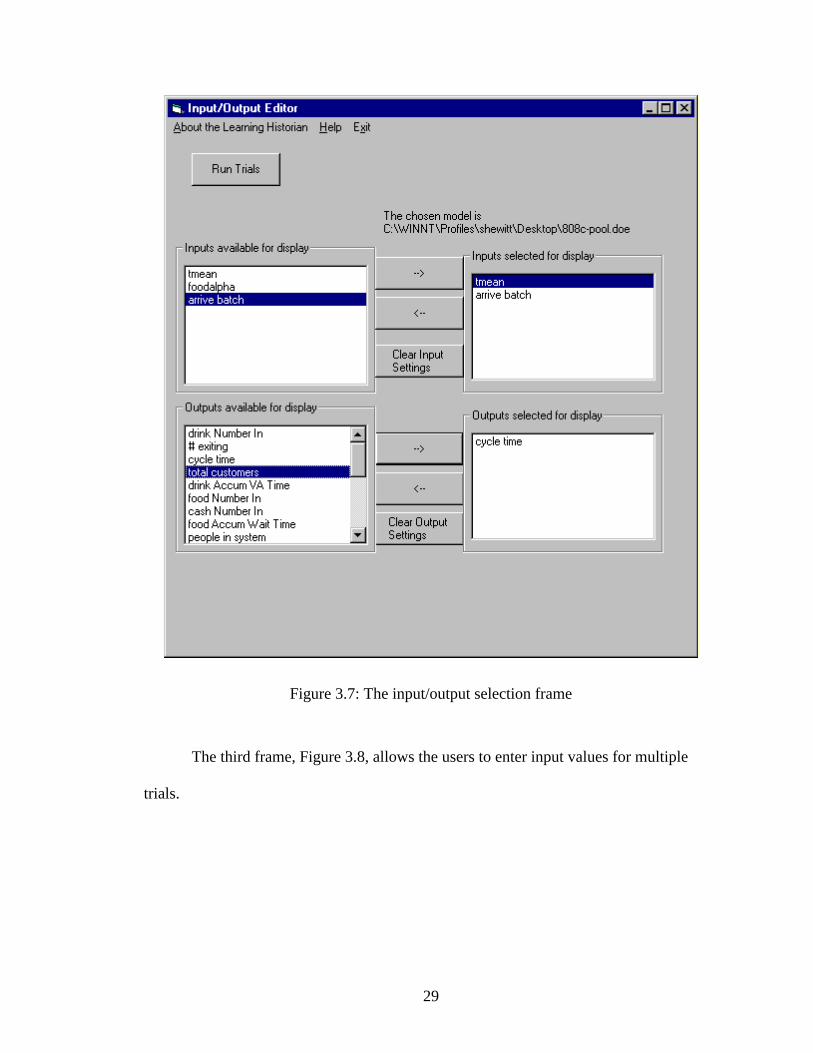
Figure 3.7: The input/output selection frame

The third frame, Figure 3.8, allows the users to enter input values for multiple

trials.

30

Figure 3.8: The trials screen

The fourth frame, Figure 3.9, is Spotfire, which graphs the trials. Each trial is

represented as a data point in Spotfire. Spotfire allows the user to change the axis of the

graphs and to filter results in order to more closely analyze different components of the

system.

31

Figure 3.9: A graph produced by Spotfire

For more information about the Learning Historian please see Appendix A.

3.6 Summary

An analytical model and an Arena model of a manufacturing system and a push-

pull system will form the basis of the experimentation for the difference between

analytical models and discrete event simulation models. Each model will be run for a

variety of input values, these results will be compared to determine the difference

between the analytical model and the Arena model.

One tool in this process will be a Learning Historian that sits on top of the Arena

model. The Learning Historian facilitates simulation by making it faster and easier for

32

users to run multiple trials by automatically recording output results and by incorporating

a method of visualizing multiple results.

This Learning Historian uses many of the components of the VisSim continuous

time simulation developed by the Human Computer Interaction Laboratory (HCIL). The

HCIL Learning Historian was modified to reflect the behavior and simulation capabilities

of a discrete-event simulation. After a preliminary version of the Learning Historian was

developed, various usability studies were conducted to improve the Arena Learning

Historian.

The Learning Historian is written in Visual Basic because the Arena program uses

a Visual Basic interface. The Learning Historian works by writing the user-defined

inputs to a temporary text file, the Arena program then modifies the Arena model with

the new input values, runs the Arena model and the Learning Historian parses the Arena

generated output file for the output results and their half-widths. The results and the half-

widths are displayed in the Learning Historian in a chart and in a comma-delimited file

that can be saved and that can be opened using a visual data-mining tool called Spotfire.

33

4 A simple queueing system

4.1 Introduction

In order to more clearly explain the methodology that will be used in the following

chapters, this chapter presents an example of a simple queuing system. The results from

the analytical equations and the Arena model are presented and compared and any

discrepancies discussed.

4.2 M/M/1 Queuing

Queuing systems are described by their arrival rate, processing rate and the

number of servers in the system. The M denotes Markovian behavior, which signifies an

exponential distribution. Therefore, an M/M/1 system has exponentially distributed

interarrival times, an exponentially distributed service time and one server. The arrival

rate is denoted by � and the service rate is �. The unit for rates is customers per hour.

The mean interarrival time is equal to 1/� and the mean processing time is equal to 1/�.

If the arrival rate, �, is greater than the service rate, �, that is, if, on average, the

system creates entities faster than the system can process the entities, the system will not

reach steady state. The system will be examined for a variety of utilization levels,

achieved by varying either the arrival rate, �, or the service rate, ���Banks et al., 2001).

4.3 Analytical model

The following variables and equations are used in the calculations of the

analytical model.

Let � be the utilization of the server.

34

��

� �

Let Lq be the average number of customers in queue. Let Ls be the average

number of customers in the system. The following equations can be used to calculate Lq

and Ls (Banks et al., 2001):

��

��

��

��

1

1

2

s

q

L

L

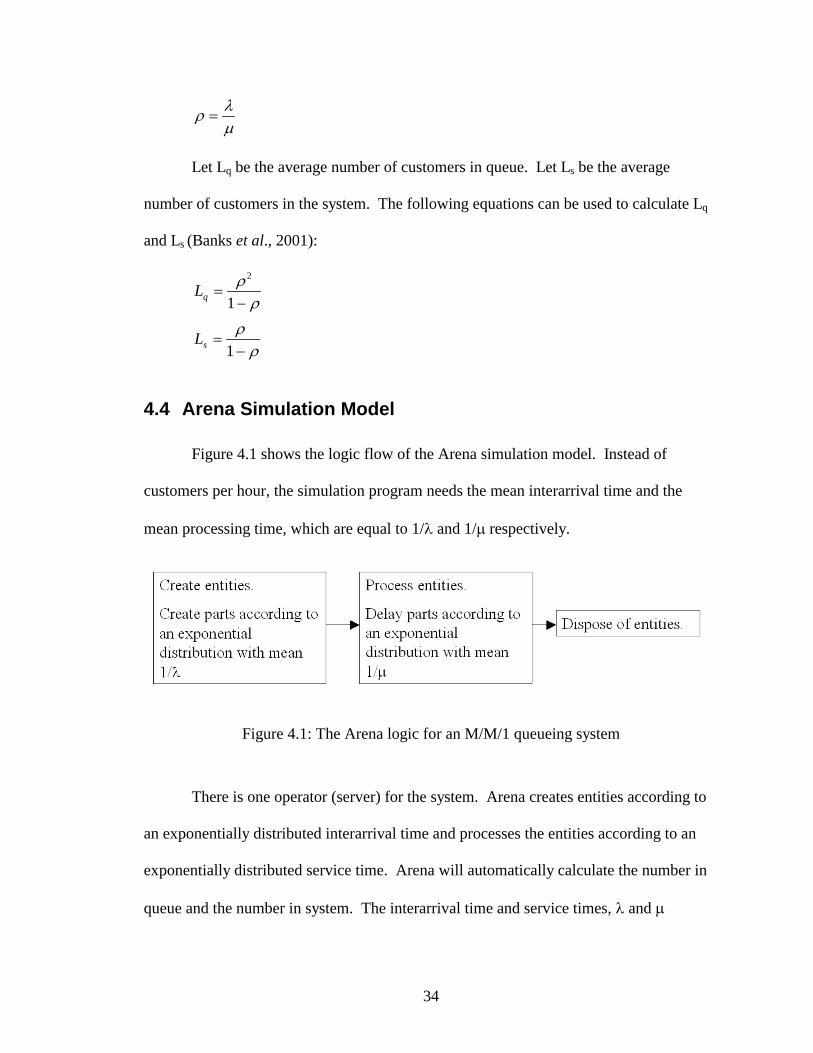
4.4 Arena Simulation Model

Figure 4.1 shows the logic flow of the Arena simulation model. Instead of

customers per hour, the simulation program needs the mean interarrival time and the

mean processing time, which are equal to 1/� and 1/� respectively.

Figure 4.1: The Arena logic for an M/M/1 queueing system

There is one operator (server) for the system. Arena creates entities according to

an exponentially distributed interarrival time and processes the entities according to an

exponentially distributed service time. Arena will automatically calculate the number in

queue and the number in system. The interarrival time and service times, � and �

35

respectively, are defined as variables so that the model can be run with the Learning

Historian.

4.5 Results and Discussion

The following is a list of input values for � and � and the output results for both

the analytical model and the Arena model. The Learning Historian collected the results

of the Arena simulation. The Arena results represent a 95% confidence interval, using

data from ten trials of 1500 minutes, with the results of the first 100 minutes ignored due

to initial transient effects. The number in queue and the average queue time are related

by Little’s Law (this was checked during the validation of the model), therefore only the

results of the number in queue and the number in the system (work-in-progress) are

shown in the table below.

Number in System (Ls) Number in Queue (Lq)

�� �� Analytical Simulation Analytical Simulation 20 10 1.0000 0.9856 ± 0.0215 0.5000 0.4884 ± 0.0175 30 10 0.5000 0.4960 ± 0.0058 0.1667 0.1640 ± 0.0044 40 10 0.3333 0.3325 ± 0.0049 0.0833 0.0829 ± 0.0030 50 10 0.2500 0.2487 ± 0.0025 0.0500 0.0495 ± 0.0014 60 10 0.2000 0.1991 ± 0.0020 0.0333 0.0329 ± 0.0011 70 10 0.1667 0.1666 ± 0.0020 0.0238 0.0240 ± 0.0009 80 10 0.1429 0.1422 ± 0.0016 0.0179 0.0176 ± 0.0008 90 10 0.1250 0.1246 ± 0.0014 0.0139 0.0138 ± 0.0006 100 10 0.1111 0.1107 ± 0.0011 0.0111 0.0109 ± 0.0005 100 20 0.2500 0.2505 ± 0.0024 0.0500 0.0503 ± 0.0010 100 30 0.4286 0.4275 ± 0.0024 0.1286 0.1284 ± 0.0013 100 40 0.6667 0.6660 ± 0.0050 0.2667 0.2656 ± 0.0034 100 50 1.0000 0.9993 ± 0.0110 0.5000 0.4983 ± 0.0094 100 60 1.5000 1.5026 ± 0.0197 0.9000 0.9029 ± 0.0172 100 70 2.3333 2.3337 ± 0.0250 1.6333 1.6352 ± 0.0224 100 80 4.0000 4.0127 ± 0.0792 3.2000 3.2116 ± 0.0767 100 90 9.0000 9.0430 ± 0.3446 8.1000 8.1430 ± 0.3425

Table 4.1: Summary of results for an M/M/1 queueing system

36

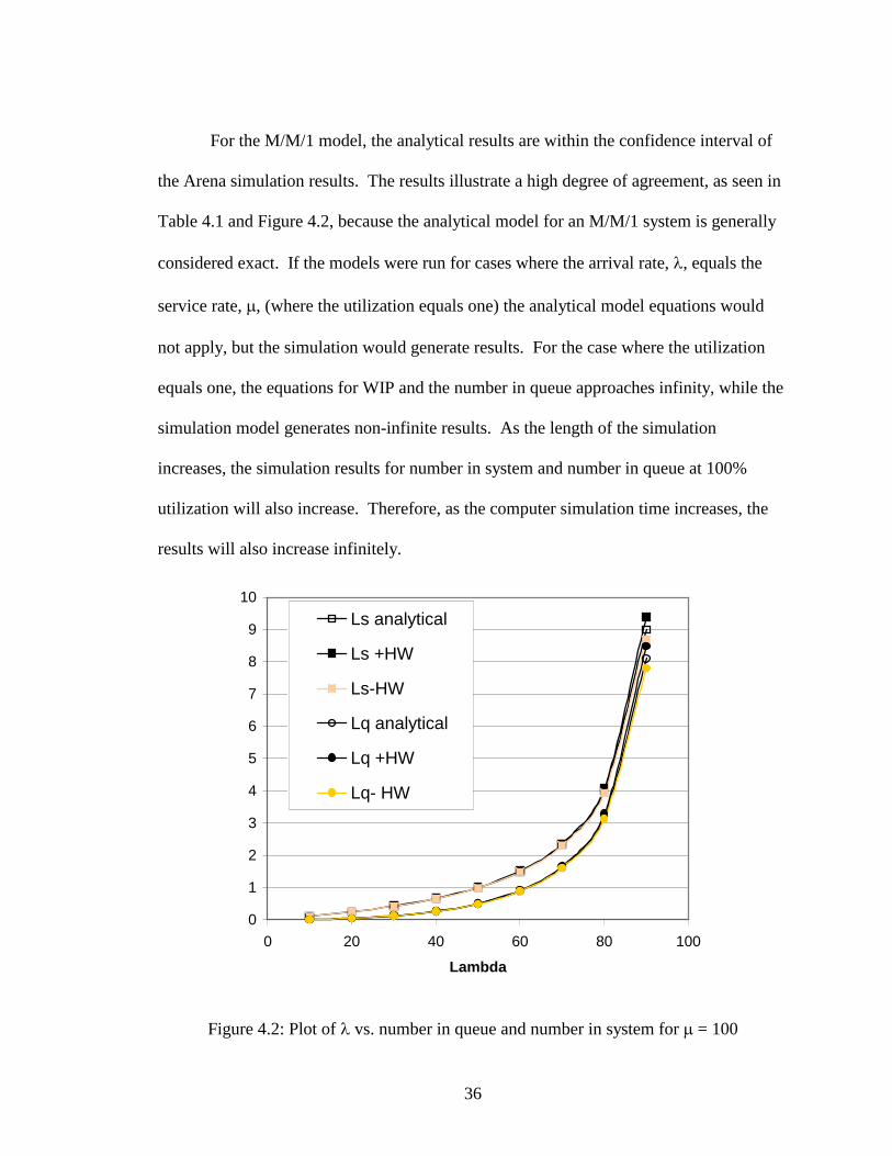
For the M/M/1 model, the analytical results are within the confidence interval of

the Arena simulation results. The results illustrate a high degree of agreement, as seen in

Table 4.1 and Figure 4.2, because the analytical model for an M/M/1 system is generally

considered exact. If the models were run for cases where the arrival rate, �, equals the

service rate, �, (where the utilization equals one) the analytical model equations would

not apply, but the simulation would generate results. For the case where the utilization

equals one, the equations for WIP and the number in queue approaches infinity, while the

simulation model generates non-infinite results. As the length of the simulation

increases, the simulation results for number in system and number in queue at 100%

utilization will also increase. Therefore, as the computer simulation time increases, the

results will also increase infinitely.

0

1

2

3

4

5

6

7

8

9

10

0 20 40 60 80 100

Lambda

Ls analytical

Ls +HW

Ls-HW

Lq analytical

Lq +HW

Lq- HW

Figure 4.2: Plot of � vs. number in queue and number in system for ��= 100

37

4.6 Summary

The above analysis of the M/M/1 system serves as an example of the

methodology that will be followed in the next two chapters. The Learning Historian was

used to quickly and efficiently gather the results from the Arena model. The analytical

results and the computer simulation results match within a 95% confidence interval. The

one exception to this statement is the case where the utilization equals one, at which point

the equations for the analytical model yield infinity. When the utilization is one the

simulation model will generate finite results, but the results will be dependent on the

length of the simulation run.

38

5 A flow shop with process drift

5.1 Introduction

This chapter presents the evolution of a flow shop manufacturing process model.

The results from the analytical equations and Arena are presented and compared and any

discrepancies discussed.

One of the key aspects of this manufacturing system is the role of defects and

subsequently the process yields. The yield of a process is the number of good parts

leaving the process divided by the number of good incoming parts and is expressed as a

percent. As machines process raw materials, the machine will occasionally drift out of

control. If a processing step is out of control, the yield of that step is reduced. Inspection

stations throughout the system remove the defects and serve to identify and fix the out of

control machines.

5.2 Flow Shop Example

Figure 5.1 shows the routing for a nine-step manufacturing process. Different

product lines have different processing times at each step, but follow the same routing

through the system. The processing times for Electroless plating and Electroplating, are

independent of the batch size; all other processing times depend on the size of the batch

at the station.

39

Figure 5.1: The product routing for the process flow example

Steps 1, 3, 4, 5, 7, and 8 are manufacturing stations. Each manufacturing station

can either be within specified parameters (in-control) or out-of-control. In this example,

an in-control process has a 98% yield and an out-of-control process has a 70% yield.

Each manufacturing step has a drift rate that determines the frequency with which the

step goes out-of-control. If a manufacturing step goes out-of-control, it will be corrected

when the drift is detected at the next inspection station, as shown in Figure 5.2.

Station 1 Inspect 1 Defect arrives Part a arrives. Processed at reduced yield

Part a finishes processing Part a arrives at Inspect 1 and begins processing

Part b arrives. Processed at reduced yield

Part a finishes inspection. Defect detected and corrected

Part b finishes processing Part b arrives at Inspect 1 Part c arrives. Processed at non-reduced yield

Figure 5.2: Sample timeline of events

40

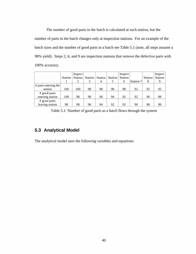
The number of good parts in the batch is calculated at each station, but the

number of parts in the batch changes only at inspection stations. For an example of the

batch sizes and the number of good parts in a batch see Table 5.1 (note, all steps assume a

98% yield). Steps 2, 6, and 9 are inspection stations that remove the defective parts with

100% accuracy.

Station

1

Inspect Station

2 Station

3 Station

4 Station

5

Inspect Station

6 Station 7 Station

8

Inspect Station

9 # parts entering the

station 100 100 98 98 98 98 92 92 92 # good parts

entering station 100 98 98 96 94 92 92 90 88 # good parts

leaving station 98 98 96 94 92 92 90 88 88

Table 5.1: Number of good parts as a batch flows through the system

5.3 Analytical Model

The analytical model uses the following variables and equations:

41

The delay between a process going out of control and detection of the out of

control process is a function of the cycle time at each step between the out-of-control step

and the inspection station.

*

*

Squared Coefficient of variation (SCV) of interarrical times at station

SCV of the modified aggregate process time

the average cycle time of jobs of product

the average cycle time at

aj

j

i

j

c j

c

CT i

CT

�

�

�

�

*

station

expected delay in detection of a process drift in product

occurring at station ,

expected delay in detection of a process drift at station ,

the set of all inspectio

=ij

i

j

j

DT i

j j R J

DT j j J

F

�

� �

� �

� n stations

( , ) station that product visits immediately before station

1, ,

the set of all processing stations

number of resources at station

sequence of stations that product j

i

H i j i j

j i I i j n

J

n j

R i

�� � � � � ���

�

*

must visit

subsequence of , that starts with the station that follows

and ends with the next inspection station for

{ 1, , };

modified aggregate process time at station

the

=

ij i

i

j

j

Q R j

j R J

j m m F

t j

u

�

� �� � �

�

�

�

average resource utilization at station

normal unchecked yield of product at station

reduced unchecked yield of product at station

average unchecked yield due to drift for product

nij

rij

ij

j

y i j

y i j

z

�

�

� at station

process drift rate for station j

i j

j� �

*

*

;

min{ };

ij

j

ij g ig Q

j iji V

DT CT j R J

DT DT j J

�

�

� � � �

� � �

42

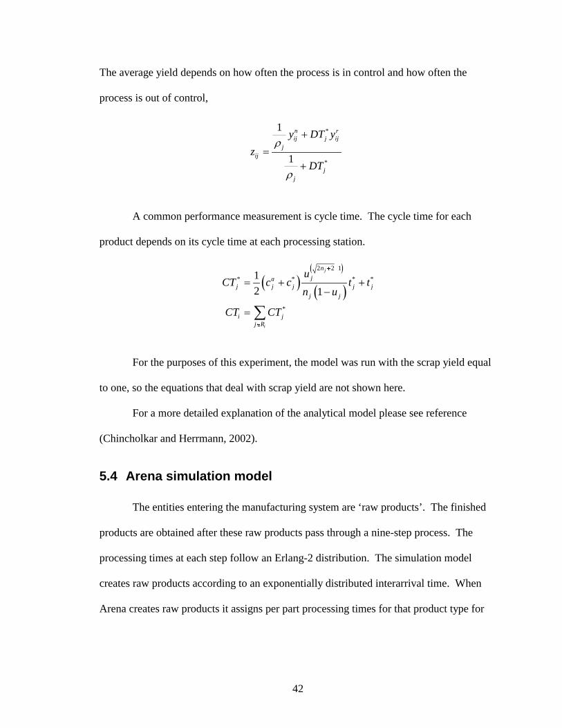
The average yield depends on how often the process is in control and how often the

process is out of control,

A common performance measurement is cycle time. The cycle time for each

product depends on its cycle time at each processing station.

For the purposes of this experiment, the model was run with the scrap yield equal

to one, so the equations that deal with scrap yield are not shown here.

For a more detailed explanation of the analytical model please see reference

(Chincholkar and Herrmann, 2002).

5.4 Arena simulation model

The entities entering the manufacturing system are ‘raw products’. The finished

products are obtained after these raw products pass through a nine-step process. The

processing times at each step follow an Erlang-2 distribution. The simulation model

creates raw products according to an exponentially distributed interarrival time. When

Arena creates raw products it assigns per part processing times for that product type for

*

*

1

1

n rij j ij

jij

jj

y DT y

zDT

�

�

�

��

� �� �

� �

2 2 1

* * * *

*

1

2 1

j

i

n

jaj j j j j

j j

i jj R

uCT c c t t

n u

CT CT

� �

�

� � ��

�

43

each station in the system and a batch size specifying the number of raw products in the

batch. The products are then routed to the first manufacturing station.

This Arena model creates defects as entities that trigger a process to become out-

of-control. Arena creates defects according to an exponentially distributed interarrival

time with a mean equal to one divided by the drift rate (1/�j). Each step has its own drift

rate, so each step has its own different type of defect entity; that is, the defect that causes

step three to go out-of-control is different and independent of the defect that will cause

step four to go out-of-control. When Arena creates a defect, the defect immediately

travels from the create block to the station that the defect will cause to go out-of-control

(see Figure 5.3). When a defect is detected, the inspection station fixes only that defect;

if there are multiple defects at a station when one defect is detected, only one of the

defects is corrected.

There is a defect counter for each processing step. As mentioned before, a

different type of defect entity affects each step. Therefore, the defect counter for

processing step three only counts the step three defects in the system while the defect

counter for step four only counts the step four defects in the system and so on. When a

defect arrives at a station, the defect counter for that station is incremented by one. A

manufacturing step is deemed to be out-of-control whenever its defect counter is greater

than or equal to one. The defect remains at the station until a raw product arrives at the

station. When the raw product arrives, it checks to see if there are any defects waiting at

the station. If there are no waiting defects, the raw product is processed and continues

through the system. If there is a defect waiting at the station, the defect entity is “joined”

to the raw product. The joined raw product and defect entity is akin to a sticker being

44

placed on the raw product indicating that the step is out-of-control. The raw product and

the defect now go through the system together, obeying the processing times and rules for

the raw product (see Figure 5.4).

At an inspection station the raw product and defect are delayed for a specified

inspection processing time. The raw product and defect are then split apart and travel

through a series of logic blocks that identify defect entities. Whenever the logic blocks

detect a defect entity, they pull the defect out of the system, decrease the appropriate

defect counter by one and dispose of the defect (see Figure 5.5).

The number of good products in a batch is recalculated at each step. The

calculation is a function of the previous number of good products in the batch and the

yield of the step, which depends on whether or not the step is out of control. The number

in the batch is recalculated only at inspection stations.

� �1

j

number of good parts leaving workstation j

number of good parts entering workstation j

number of output good parts = number of input good parts

y fractional yield at workstation j

j

j

b

b

x P

�

�

�

�

�

The Arena model and the analytical model use a simplistic calculation of:

� �� �1 j j jb b y�

� . (Another method of calculating the number of good parts in a batch

would be to use the binomial distribution. This might be more valid in some settings, but

it is not available in the Arena program).

The Arena model needs the batch size to be an integer number, but often the

number of good parts in a batch will equal a fractional batch size. For example, if the

batch size is 98 and the yield is 98%, the expected number of good parts in a batch is

(0.98)(98)=96.04. However, the Arena model needs the number good in the batch to be

45

an integer number, so Arena will treat 96.04 as 96, thereby reducing the yield to 97.96%

instead of 98%. In order to create integer numbers for the number of good parts in a

batch, and maintain the correct yield, the number of good parts in the batch is calculated

using a modified formula. This modified expression calculates the number of good parts

in a batch, bj, as either the rounded down integer value of � �� �1 j j jb b y�

� , or as the

batch size 1j jb b�

� . The batches will use the 100% yield calculation a fraction of the

time and will use the integer value of � �� �1j jb y�

the rest of the time. The Arena model

implements this by having each batch go through a probability module that determines if

the batch will be multiplied by a fractional yield or by a 100% yield. The probability

module is re-evaluated for each batch that passes through the probability module. The

chance x that 1j jb b�

� is determined for each batch according to the algorithm below:

Using an example of a batch size of 100 and a yield of 98%, the expression is

evaluated as follows:

Check: � �� � � �� � � �� �10.02 98 0.98 96 96.04 j jb y�

� � �

� �� � � � � �� �� � � �� �� � � � � �� � � �� �� � � �� �

� �� �� � � �� � � �� �� � � � � �� �� �

� �� �

1 1 1

1 1 1 1

1 1 1 1

1 1

1 1

1 integer

integer integer

- integer integer

integer

integer

j j j j j

j j j j j j j

j j j j j j j

j j j j

j j j

x b x b y b y

x b b y x b y b y

x b b y b y b y

b y b yx

b b y

� � �

� � � �

� � � �

� �

� �

� �� � �� �

� � � �� � �� � � �

� � � �� �� � � �

� � � ��� � � � �� �� � �

� �� � � �� �

� �

0.98 98 96.04

integer(96.04) 96

96.04 960.02

98 96

j jb y

x

� �

�

�� �

�

46

Figu

re 5

.3: C

reat

ing

and

rout

ing

a de

fect

Pro

cess

Is p

roce

ss b

ad?

Def

ect o

r par

t?

Is a

def

ect w

aitin

g?

part

Join

def

ect a

nd

batc

hA

ssig

n #

goo

d in

Rou

te to

nex

t ste

p

Cou

nt

batc

hA

ssig

n #

good

in

Cou

nt

Fi

gure

5.4

: Log

ic a

t a p

roce

ss s

tep

Sta

tion

Ins

pe

ctio

np

rod

uc

tsg

et r

id o

f ba

dD

isp

os

e o

f De

fec

t

P1

oo

c

Cou

nta

nd

De

fec

tsS

ep

ara

te P

art

sF

ix D

efe

ct

step

Send

par

t to

next

Figu

re 5

.5: I

nspe

ctio

n st

atio

n lo

gic

46

47

5.5 The role of underlying assumptions

The preliminary model exhibited large errors between the analytical results and the

simulation results, as shown in the tables below. The Learning Historian collected the

Arena results, which represent a 95% confidence interval, using data from twenty trials of

200,000 minutes, with no warm-up period. In the subsequent experiments, the input

variables that will be modified are the batch size, and the arrival rate (throughput level) of

the raw parts. Three different throughput levels are used in the following experiments.

The throughput level specifies how many Product One, Two and Three entities are

released into the system each day. The experiments are run for three different input batch

size levels. The initial batch sizes are shown in the tables below according to the

following format: the initial batch size of Product One, the initial batch size of Product

Two, the initial batch size of Product Three.

The cycle time and throughput of each product depends on the batch size at each

step, so the batch size is the output parameter of interest. The batch sizes change at the

three inspection stations: Inspect 1, Inspect 2 and Test and Tune. The Test and Tune

station is the last station in the process flow and so the batch sizes from this step are

considered the output batch size. The error between the analytical results and the

simulation results is calculated as follows:

� �analytical result-simulation result% error

simulation result�

The batch sizes at Inspect 1 for the different trials are shown in Table 5.2. At this

station, the results from the analytical model have percent errors ranging from 6.5% to

8.3%. All values are outside of the 95% confidence intervals. The batch sizes continue

48

to move farther away from the simulation results, culminating in percent errors ranging

from 34.8% to 51.8% at the Test and Tune Output station, as shown in Table 5.3.

Batch size of Product One Batch size of Product Two Batch size of Product Three TH

level Analytical Simulation Analytical Simulation Analytical Simulation

Input batch size = 50, 100, 150

1 40.506 37.772 ± 0.237 81.012 75.512 ± 0.485 121.518 113.100 ± 0.649

2 40.505 38.008 ± 0.233 81.011 75.900 ± 0.469 121.516 114.090 ± 0.747

3 40.248 37.632 ± 0.249 80.495 75.283 ± 0.503 120.743 112.780 ± 0.752

Input batch size = 100, 200, 300

1 76.939 71.221 ± 0.296 153.877 142.320 ± 0.666 230.816 213.800 ± 0.908

2 76.938 71.015 ± 0.221 153.876 142.180 ± 0.484 230.814 213.090 ± 0.745

3 76.644 71.097 ± 0.211 153.287 142.190 ± 0.391 229.931 213.470 ± 0.674

Input batch size = 150, 300, 450

1 112.598 105.420 ± 0.167 225.195 210.920 ± 0.379 337.793 316.200 ± 0.575

2 112.597 105.320 ± 0.164 225.194 210.600 ± 0.290 337.791 315.890 ± 0.525

3 112.267 105.340 ± 0.161 224.534 210.670 ± 0.329 336.802 316.030 ± 0.507

Throughput levels: 1=500, 500, 250; 2=1000, 1000, 500; 3=1500, 1500, 1000

Table 5.2: Batch size at Inspect 1 (parts per batch)

Batch size of Product One Batch size of Product Two Batch size of Product Three

TH level Analytical Simulation Analytical Simulation Analytical Simulation

Input batch size = 50, 100, 150

1 11.294 7.457 ± 0.068 22.588 15.368 ± 0.138 33.882 23.191 ± 0.227

2 11.286 7.538 ± 0.062 22.572 15.590 ± 0.123 33.857 23.609 ± 0.193

3 10.925 7.195 ± 0.055 21.849 14.903 ± 0.110 32.774 22.607 ± 0.188

Input batch size = 100, 200, 300

1 18.207 12.334 ± 0.098 36.414 25.467 ± 0.166 54.621 38.265 ± 0.329

2 18.206 12.283 ± 0.077 36.411 25.350 ± 0.133 54.617 38.162 ± 0.222

3 17.955 12.313 ± 0.065 35.910 25.396 ± 0.141 53.865 38.212 ± 0.212

Input batch size = 150, 300, 450

1 24.565 17.622 ± 0.078 49.131 35.976 ± 0.108 73.696 54.057 ± 0.296

2 24.565 17.629 ± 0.097 49.129 35.985 ± 0.178 73.694 54.297 ± 0.306

3 24.308 17.607 ± 0.058 48.616 35.886 ± 0.107 72.923 54.080 ± 0.156

Throughput levels: 1=500, 500, 250; 2=1000, 1000, 500; 3=1500, 1500, 1000

Table 5.3: Batch sizes at Test and Tune Output Station (parts per batch)

Such a large disagreement in results necessitates a careful review of the model. A

potential source of error between two models is that the two systems may use subtly

49

different underlying assumptions. Different assumptions do not always result in large,

eye-catching discrepancies; they can sometimes result in small, subtle errors that do not

necessarily attract attention. Divergent underlying assumptions can result from having

one person make the simulation model and having one person make another model, or

from having one person make the simulation model and having someone else revise the

model. Chance et al. (1999) provides an example of how assumptions, considered basic

to the original modeler, are often unknown to others.

All models utilize assumptions and as such can all fall prey to differing

assumptions about the system behavior. In this model, the treatment and behavior of the

defects is one such possible area for different assumptions. For example, if the defect

correction is presumed to correct all of the defects acting on one machine, or if no more

defects arrive once a machine is considered out of control, then the system can be

modeled as a finite state system, as shown in Figure 5.6, where the state is the number of

defects acting on a machine at a given time. The analytical model uses the finite state

assumption.

Figure 5.6: Finite State System

If, however, it is presumed that defects are unique; one defect correction only

fixes one defect at a time, then the system will be an infinite state system. An infinite

state system, where the state is the number of defects acting on a machine at a given time,

50

is shown in Figure 5.7. The preliminary version of the Arena model used the infinite

state assumption.

Figure 5.7: Infinite State System

If modeled as a finite state system, a workstation j will have an average yield of:

*j

j

*j

j

1DT

1DT

n rj jy y

�

�

�

�

If modeled as an infinite state system, the workstation will have a yield of:

� �� � � �* * *j j j j j j1 DT DT , DT <1n r

j jy y� � �� �

For trials where defects are fixed faster than they arrive, that is, where defects are

fixed before the next defect would arrive, both the infinite and finite state systems will

result in the same effective yield. If, however, defects arrive faster than they are

detected, then the infinite state system will not reach steady state and the average yield of

the infinite state will approach its lower limit, equal to the reduced yield. To fix the

discrepancy, the simulation model was modified to be a finite state system so that only

one defect can act on a station at a time; no more defects arrive while the machine is

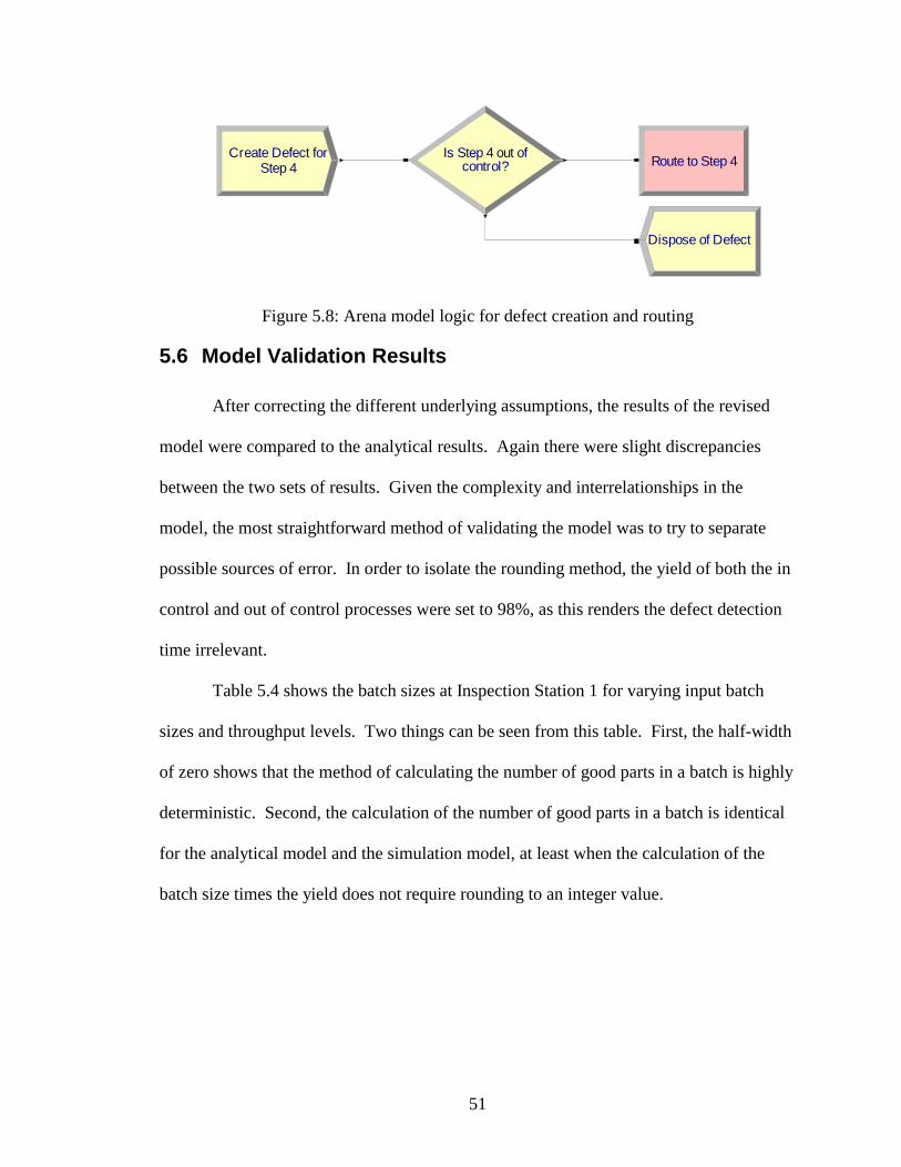
considered out of control. The revised model uses the logic shown in Figure 5.8 for the

defect creation and routing; this is a change from the logic shown earlier in Figure 5.3.

51

Step 4Create Defect for

control?Is Step 4 out of

Dispose of Defect

Route to Step 4

Figure 5.8: Arena model logic for defect creation and routing

5.6 Model Validation Results

After correcting the different underlying assumptions, the results of the revised

model were compared to the analytical results. Again there were slight discrepancies

between the two sets of results. Given the complexity and interrelationships in the

model, the most straightforward method of validating the model was to try to separate

possible sources of error. In order to isolate the rounding method, the yield of both the in

control and out of control processes were set to 98%, as this renders the defect detection

time irrelevant.

Table 5.4 shows the batch sizes at Inspection Station 1 for varying input batch

sizes and throughput levels. Two things can be seen from this table. First, the half-width

of zero shows that the method of calculating the number of good parts in a batch is highly

deterministic. Second, the calculation of the number of good parts in a batch is identical

for the analytical model and the simulation model, at least when the calculation of the

batch size times the yield does not require rounding to an integer value.

52

Batch Size of Product

One Batch Size of Product

Two Batch Size of Product

Three Throughput (TH) Level Analytical Simulation Analytical Simulation Analytical Simulation

Input Batch Size = 50, 100, 150 1 49 49 ± 0 98 98 ± 0 147 147 ± 0 2 49 49 ± 0 98 98 ± 0 147 147 ± 0 3 49 49 ± 0 98 98 ± 0 147 147 ± 0

Input Batch Size = 100, 200, 300 1 98 98 ± 0 196 196 ± 0 294 294 ± 0 2 98 98 ± 0 196 196 ± 0 294 294 ± 0 3 98 98 ± 0 196 196 ± 0 294 294 ± 0

Input Batch Size = 150, 300, 450 1 147 147 ± 0 294 294 ± 0 441 441 ± 0 2 147 147 ± 0 294 294 ± 0 441 441 ± 0 3 147 147 ± 0 294 294 ± 0 441 441 ± 0 Throughput levels: 1=500, 500, 250; 2=1000, 1000, 500; 3=1500, 1500, 1000

Table 5.4: Batch sizes at Inspection Station 1

Table 5.5, batch sizes at Inspection Station 2, highlights a new facet of the yield

calculations; the situation where the yield times the batch size is not equal to an integer

number. At this point it is necessary to use the modified formula mentioned above. For

the case with input batch sizes of 100, 200, 300, 2% of the batches should have 100%

yield at station 3, Electroless Plating, because,

96.04 96 192.08 192 288.12 2880.02

98 96 196 192 294 288

� � �� � �

� � �

53

Batch Size of Product One Batch Size of Product Two Batch Size of Product Three TH

level Analytical Simulation Analytical Simulation Analytical Simulation

Input Batch Size=50, 100, 150

1 46.118 46.059 ± 0.00199 92.237 92.117 ± 0.00561 138.355 138.160 ± 0.01377

2 46.118 46.060 ± 0.00167 92.237 92.120 ± 0.00269 138.355 138.170 ± 0.00870

3 46.118 46.060 ± 0.00065 92.237 92.119 ± 0.00324 138.355 138.170 ± 0.00702

Input Batch Size=100, 200, 300

1 92.237 92.122 ± 0.00420 184.474 184.240 ± 0.01328 276.710 276.350 ± 0.03486

2 92.237 92.118 ± 0.00388 184.474 184.240 ± 0.00831 276.710 276.360 ± 0.03157

3 92.237 92.121 ± 0.00262 184.474 184.230 ± 0.01034 276.710 276.360 ± 0.01598

Input Batch Size=150, 300, 450

1 138.355 138.180 ± 0.00972 276.710 276.340 ± 0.03376 415.066 414.600 ± 0.06942

2 138.355 138.180 ± 0.00540 276.710 276.360 ± 0.01889 415.066 414.520 ± 0.04638

3 138.355 138.180 ± 0.00565 276.710 276.350 ± 0.01844 415.066 414.510 ± 0.04068

Throughput levels: 1=500, 500, 250; 2=1000, 1000, 500; 3=1500, 1500, 1000

Table 5.5: Batch sizes at Inspection Station 2

Measuring which percent of batches use a 100% yield and which percent of

batches use a 98% yield validates the simulation model logic. Taking a typical scenario

from the above trials (input batch sizes = 100, 200, 300; throughput equals 1500, 1500,

1000; 20 replications; 200,000 minutes per replication), the twenty averages are shown in

Figure 5.8. The average of the twenty values is shown as a solid horizontal line in the

figure. After the probability block, the batches pass through blocks that assign a new

number of good parts per batch. After the assignment of a new number of good parts per

batch there are counters that measure how many batches went through blocks that

assigned 1 j jb b�

� , and how many batches went through blocks that assigned

� �� �j j-1 ijb =integer b y� �� . The values in Figure 5.9 come from the counters that follow the

probability block.

54

0.0185

0.019

0.0195

0.02

0.0205

0.021

0.0215

0.022

0.0225

Figure 5.9: Scatter plot of probability results

Using a 95% confidence interval, the average of the twenty replications is

0.02031 ± 0.00031. The desired value of 0.02 falls within this confidence interval, so the

probability module is working correctly. Given that Table 5.4 shows that the model

correctly calculates the value of yield times batch size, it is reasonable to assume that the

error in batch sizes between the analytical model and the simulation model are due to the

variability in the probability distribution and the random nature of the simulation. The

difference in effective yields between the analytical model and the simulation model

ranges from 0.12% to 0.13% for the situation where all of the reduced yields are set to

98%, and from 0.7% to 4.4% when all of the reduced yields are set to 70%.

It is also necessary to note that while the analytical model and the simulation

model appear to be in agreement when the all of the yield rates are 98% (the batch sizes

differ by 0.11% to 0.14%), the confidence interval is very small, and consequently the

analytical model is outside of the confidence interval of the simulation model.

55

The results at the Test and Tune Station, the output station, demonstrate the same

rounding errors as seen above for the situation where all of the yields are set to 98%. The

rounding error propagates, however, and the percent error between the analytical model

batch sizes and the simulation model batch sizes ranges from 0.13% to 0.18%. Again,

these values are outside of the confidence intervals for the simulation model.

5.7 Results

Now that the underlying assumptions of the two models are in agreement, and the

behavior of the probability block has been studied, the two models should produce

similar results, at least within confidence intervals. The Arena model was run using the

same parameters as mentioned in Section 5.5

The Batch sizes for the different trials at Inspection Station 1 are shown in Table

5.6. At this station the results from the analytical model are within 0.38% of the average

simulation result, which is within the 95% confidence interval of the simulation results.

Batch Size of Product One Batch Size of Product Two Batch Size of Product Three TH level Analytical Simulation Analytical Simulation Analytical Simulation

Input Batch Size=50, 100, 150 1 40.506 40.442± 0.217 81.012 80.953± 0.445 121.518 121.540±0.903 2 40.505 40.461± 0.236 81.011 80.836± 0.538 121.516 121.360±0.823 3 40.248 40.163± 0.149 80.495 80.348± 0.284 120.743 120.440±0.447

Input Batch Size=100, 200, 300 1 76.939 77.027± 0.586 153.877 153.810± 1.208 230.816 231.700±1.918 2 76.938 77.236± 0.442 153.876 154.380± 0.827 230.814 232.030±1.369 3 76.644 76.428± 0.385 153.287 152.780± 0.767 229.931 229.040±1.402

Input Batch Size=150, 300, 450 1 112.598 112.680± 0.589 225.195 225.220± 1.251 337.793 337.530±2.087 2 112.597 112.580± 0.579 225.194 225.330± 1.318 337.791 336.760±2.080 3 112.267 112.050± 0.626 224.534 223.920± 1.166 336.802 336.190±1.818

Throughput levels: 1=500, 500, 250; 2=1000, 1000, 500; 3=1500, 1500, 1000

Table 5.6: Batch sizes at Inspection Station 1

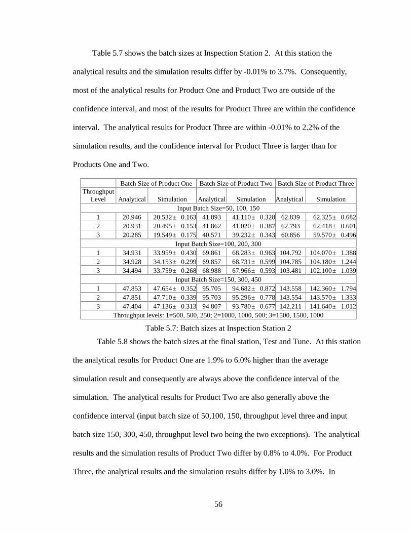
56

Table 5.7 shows the batch sizes at Inspection Station 2. At this station the

analytical results and the simulation results differ by -0.01% to 3.7%. Consequently,

most of the analytical results for Product One and Product Two are outside of the

confidence interval, and most of the results for Product Three are within the confidence

interval. The analytical results for Product Three are within -0.01% to 2.2% of the

simulation results, and the confidence interval for Product Three is larger than for

Products One and Two.

Batch Size of Product One Batch Size of Product Two Batch Size of Product Three Throughput

Level Analytical Simulation Analytical Simulation Analytical Simulation Input Batch Size=50, 100, 150

1 20.946 20.532± 0.163 41.893 41.110± 0.328 62.839 62.325± 0.6822 20.931 20.495± 0.153 41.862 41.020± 0.387 62.793 62.418± 0.6013 20.285 19.549± 0.175 40.571 39.232± 0.343 60.856 59.570± 0.496

Input Batch Size=100, 200, 300 1 34.931 33.959± 0.430 69.861 68.283± 0.963 104.792 104.070± 1.3882 34.928 34.153± 0.299 69.857 68.731± 0.599 104.785 104.180± 1.2443 34.494 33.759± 0.268 68.988 67.966± 0.593 103.481 102.100± 1.039

Input Batch Size=150, 300, 450 1 47.853 47.654± 0.352 95.705 94.682± 0.872 143.558 142.360± 1.7942 47.851 47.710± 0.339 95.703 95.296± 0.778 143.554 143.570± 1.3333 47.404 47.136± 0.313 94.807 93.780± 0.677 142.211 141.640± 1.012

Throughput levels: 1=500, 500, 250; 2=1000, 1000, 500; 3=1500, 1500, 1000

Table 5.7: Batch sizes at Inspection Station 2

Table 5.8 shows the batch sizes at the final station, Test and Tune. At this station

the analytical results for Product One are 1.9% to 6.0% higher than the average

simulation result and consequently are always above the confidence interval of the

simulation. The analytical results for Product Two are also generally above the

confidence interval (input batch size of 50,100, 150, throughput level three and input

batch size 150, 300, 450, throughput level two being the two exceptions). The analytical

results and the simulation results of Product Two differ by 0.8% to 4.0%. For Product

Three, the analytical results and the simulation results differ by 1.0% to 3.0%. In

57

addition, the confidence interval for Product Three is slightly larger than for Products

One or Two. As such, two of the results are within the simulation confidence intervals

and two of the results are outside of the confidence interval by only 0.07% and 0.1%.

Batch Size of Product One Batch Size of Product Two Batch Size of Product Three Throughput

Level Analytical Simulation Analytical Simulation Analytical Simulation Input Batch Size=50, 100, 150

1 11.294 10.826 ± 0.081 22.588 22.005 ± 0.160 33.882 33.188 ± 0.349 2 11.286 10.825 ± 0.077 22.572 21.984 ± 0.197 33.857 33.291 ± 0.287 3 10.925 10.302 ± 0.091 21.849 21.019 ± 0.158 32.774 31.814 ± 0.250

Input Batch Size=100, 200, 300 1 18.207 17.604 ± 0.232 36.414 35.534 ± 0.492 54.621 53.830 ± 0.824 2 18.206 17.685 ± 0.170 36.411 35.703 ± 0.348 54.617 53.926 ± 0.738 3 17.955 17.491 ± 0.142 35.910 35.374 ± 0.301 53.865 52.980 ± 0.509

Input Batch Size=150, 300, 450 1 24.565 24.072 ± 0.187 49.131 48.369 ± 0.425 73.696 72.767 ± 0.851 2 24.565 24.098 ± 0.175 49.129 48.749 ± 0.464 73.694 72.949 ± 0.692 3 24.308 23.807 ± 0.150 48.616 48.008 ± 0.311 72.923 71.966 ± 0.515

Throughput levels: 1=500, 500, 250; 2=1000, 1000, 500; 3=1500, 1500, 1000

Table 5.8: Batch Sizes at Test and Tune Output Station

5.8 Discussion

One trend in the above results is the tendency for the results of Product Three to

have a slightly larger half-width than Products One and Two. This is due in part to the

number of batches released for Product Three. Product Three has the largest batch size

and the lowest daily throughput, so there are far fewer batches per day than Product One

or Two. Fewer batches released correlates to fewer data points to average, so the Product

Three averages are more scattered, which results in a larger half-width when the results

of the twenty replications are averaged together. For example, for the 150, 300, 450 case,

with a throughput of 500, 500, 250, there are only 450/250=0.56 batches of Product

Three released per day, while there are 500/150=3.33 batches of Product One per day.

58

The Product Three confidence intervals are, at maximum, 1.2% of the average value,

which is an acceptable size for a confidence interval.

The primary source of difference between the analytic model and the simulation

model is the variability introduced by the calculation of the batch sizes. As shown in the

validation section above, both the 98% yield and the 70% yield result in a slight error in

the yield calculation. This error occurs at each station, so the errors will propagate

through the system, resulting in an increase in the batch size percent errors from Inspect 1

to the Test and Tune station.

The differences between the analytical and simulation model might be mitigated

if it were possible to calculate the batch size using a more appropriate method, such as

the Binomial distribution. Using a Binomial distribution would offer two benefits: one,

Binomial distributions would only produce integer values, which would eliminate the

errors due to rounding from the probability block. Additionally, using a more stochastic

distribution would increase the width of the confidence interval. The analytical and

simulation answers at the final station differ by 1.9% to 6.0%, but a 1.9% difference is

enough of a difference to make the analytical result outside of the confidence interval of

the simulation model.

5.9 Summary

The process flow model offers an opportunity to use the validation and verification

stages of the development of a simulation model to critically analyze model behavior.

Validation offered an opportunity to examine the underlying assumptions of the model

that could, if undetected, result in a large difference between the analytical and

59

simulation models. Verifying the batch size calculation within the model illuminated the

constant error that would exist at each batch size calculation. The constant error in the

batch size calculation, due to the variability of the probability block within the simulation

model illustrates the impact of propagation of errors within a model.

60

6 Push-pull models

6.1 Introduction

A push-pull system is a term used in operations planning and control to denote a

system that combines push production control and pull production control. In a push

system, each workstation works on the pieces waiting for processing and then “pushes”

the work to the next station, regardless of the workload of the following workstation or of

the product demand. In a pull system, work is done only when the output inventory level

drops below a predetermined level and a station requests more inventory from an

upstream workstation. Pull systems are often known as Kanban systems or Just-in-Time

(JIT) systems because workstations use Kanbans to request inventory from the prior

workstation (Kanban is a Japanese word meaning card or signal) (Slack, 1997). Push and

pull systems illustrate a tradeoff between inventory levels and cycle time.

This chapter will present a two-stage push model, a hybrid pull-push model and a

two-stage pull model for comparison.

An example of a pull-push system would be a company that processes some raw

material to an intermediate stage using pull production control. This partially processed

inventory would then be stored at the push-pull interface. The push component of the

system would be the workstations that work on the partially completed inventory only

when demand for finished inventory arrives at the push pull interface.

61

6.2 Two stage system

The customer arrival rate is denoted by and the service rate is �� at the first

station and �� at the second station. All interarrival times and service times are

exponentially distributed. The unit for rates is customers per hour. The mean interarrival

time is equal to 1/ and the mean processing time for station one is equal to 1/���and the

mean processing time for station two is equal to 1/��. There is one server at each station.

If the arrival rate, , is greater than the service rate, ���or ��, that is, if, on average,

the customers arrive faster than the stations can process them, the system will not reach

steady state �Banks et al., 2001). The system will be examined for a variety of utilization

levels, achieved by varying either the arrival rate, , or the service rates, ���and ��� The

systems that have a pull component, the system will also be examined for a variety of

Kanban levels. For a steady state system, that is where the arrival rate is less than the

service rates, the arrival rate to the second station is the same as the arrival rate to the first

station. Figures 6.1, 6.2 and 6.3 show the process flow for a two-stage push system, a

hybrid pull-push system and a two-stage pull system (Liberopoulos and Dallery, 2000).

Figure 6.1:Two-stage push system

62

Figure 6.2: Pull-push system

Figure 6.3: Two-stage pull system

6.3 Analytical model

The following variables and equations are used in the calculations of the

analytical model.

Let �n be the utilization of server n.

11 �

�� � for the first station and

22 �

�� � for the second station

The equations below apply to individual stations. For systems that combine push

and pull controls, apply the push control equations at the push stations and the pull

63

control equations at the pull stations. Given that for an n-stage system, the average

system time, ��

�n

iistotals WW

1,, , analyzing the agreement of the individual isW , eliminates

the need to explicitly measure totalsW , . Therefore, in the results that follow, the individual

system times and queue times will be studied and the sum of the system times and queue

times will not. The same logic applies to the average time in queue.

6.3.1 Push System

The following equations apply for each section of a system that uses “push”

processing, where each station is a singe server processing parts according to a first come

first serve (FCFS) protocol. Let Wq be the average amount of time in queue. Let Ws be

the average amount of time in the system. The following equations can be used to

calculate Wq and Ws (Banks et al., 2001):

� �

� ���

���

��

��

1

1

1

s

q

W

W

6.3.2 Pull System

The following equations apply for each section of a system that uses “pull”

processing (Buzacott and Shanthikumar, 1993). Let zn be the number of Kanbans

circulating through the nth station of the system. Let Ws be the average time in system.

From the point of view of the customer, the time in system and the time in queue are the

same thing because it takes the customer no time to pick up inventory; that is, the

customer has a service time of zero. If the customer has to wait for inventory to be

delivered, that waiting time will be the total time that the customer spends at that station.

64

z

bW�

� ��

�

The number of Kanbans available for the machine (which is defined as the number of

Kanbans in queue plus the number of Kanbans in process) is given by

� � � �# kanbans available 11

zE�

��

� ��

. The part processed at station 1 will use the

following equations for queue time and system time:

� �

� �� �

� �

� �

� �

2 1

2 1

2 1

= # Kanbans available- # Kanbans in process

1=

1

1

1 1

1

1

1 1

1

q

z

z

z

z

q

z

s q

L

W

W W

� ��

�

� �� �� �

� ��

� �� �

� �� � � �

�

�

�

��

�

��� �

� �

��

�

��

�

�� � � �

�

The average inventory level after a station is given by

� � � �Inventory level 11

zE z�

��

� � ��

. The number of customers/parts backlogged after

a pull station is given by 1

1

z

b bL W�

��

�

� ��

.

For a two-stage pull system, the number of Kanbans cycling through the second

processing station is equal to ’2z :

1

’2 2

1’ 12 2

1

# backlogged

1

z

z z

z z�

�

�

� �

� ��

65

6.3.3 Two-stage push model

For a two-stage pull model, the total customer cycle time equals the total part cycle time

and is given by� � � �1 2

1 1 2 2

1 1

1 1s sW W� � � �

� � �� �

. The number of parts in the system is

equal to Ls1 + Ls2, which can be found by Little’s Law. Consequently,

1 21 2

1 21 1s sL L� �� �

� � �� �

6.3.4 Hybrid pull-push model

For a hybrid pull-push model, the total customer cycle time equals

� �1

11 2

1 2 2

1

1

z

b sW W�

� � � �� � �

� �, while the number of parts in the system is given by

21 2 1

21s sL L z��

� � ��

.

6.3.5 Two-stage pull model

In the two-stage pull model, the total customer cycle time equals ’2

22

2

z

bW�

� ��

� and the

number of parts in the system is fixed at 1 2 1 2s sL L z z� � � .

6.4 Arena Simulation Model

Figure 6.4, Figure 6.5 and Figure 6.6 show the logic flow of the Arena simulation

model. Instead of customers per hour, the simulation program needs the mean

interarrival time and the mean processing time, which are equal to 1/�

66

1/��� and 1/�� respectively. There is one operator (server) for each processing station.

Arena creates entities according to an exponentially distributed interarrival time and

processes the entities according to an exponentially distributed service time. The time in

each queue and the time in each station can be determined using Arena’s tallying

capabilities. The interarrival time and service times, , ��� and ��, respectively, are

defined as variables so that the model can be run with the Learning Historian.

Figure 6.4: The Arena logic for a two-stage push system

Figure 6.5: The Arena logic for a pull-push system

67

Figure 6.6: The Arena logic for the pull-pull system

6.5 Results

The following are lists of input values for � ��� and ��, and the output results for

both the analytical model and the Arena model. The Learning Historian collected the

results of the Arena simulation. The Arena results represent a 95% confidence interval,

using data from thirty trials of 1500 minutes, with the results of the first 100 minutes

ignored due to initial transient effects. The number in queue and the average queue time

are related by Little’s Law (this was checked during the validation of the model),

therefore only the results of the time in queue and the time in process are shown in the

table below.

As discussed in Chapter 4, the system will not reach steady state if the utilization,

�� is greater than or equal to 1, therefore values of , ��� and ��, have been selected to

explore a range of utilizations for stations one and two such that ��� and ���are less than

one.

68

6.5.1 Two-stage push model

The utilization of each processing station is shown in Table 6.1. As this is a push-

push model, the equations used in the analytical model are always the push equations and

result in a high degree of agreement between the analytical and simulation model as seen

in Figure 6.7. The high degree of agreement results from the exact analytical equations.

The analytical results for utilization levels are all within 1% of the average simulation

results, which is within the 95% confidence interval of the simulation results. The cycle

times for each station are shown in Table 6.2. The analytical results for the cycle times

are within 1.9% of the average simulation results and within the 95% confidence

intervals. The queue times for each station are shown in Table 6.3. The analytical

estimates of queue times are within 2.7% of the simulation results, which is within the

95% confidence intervals.

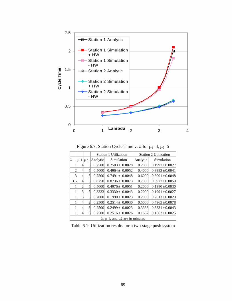
69

0

0.5

1

1.5

2

2.5

0 1 2 3 4Lambda

Cyc

le T

ime

Station 1 Analytic

Station 1 Simulation+ HWStation 1 Simulation- HWStation 2 Analytic

Station 2 Simulation+ HWStation 2 Simulation- HW

Figure 6.7: Station Cycle Time v. for �1=4, �2=5

Station 1 Utilization Station 2 Utilization

� � �� Analytic Simulation Analytic Simulation

1 4 5 0.2500 0.2503 ± 0.0028 0.2000 0.1997 ±0.0027

2 4 5 0.5000 0.4964 ± 0.0052 0.4000 0.3983 ±0.0041

3 4 5 0.7500 0.7491 ± 0.0048 0.6000 0.6001 ±0.0048

3.5 4 5 0.8750 0.8736 ± 0.0073 0.7000 0.6977 ±0.0059

1 2 5 0.5000 0.4976 ± 0.0051 0.2000 0.1980 ±0.0030

1 3 5 0.3333 0.3330 ± 0.0043 0.2000 0.1991 ±0.0027

1 5 5 0.2000 0.1990 ± 0.0023 0.2000 0.2013 ±0.0029

1 4 2 0.2500 0.2514 ± 0.0030 0.5000 0.4965 ±0.0078

1 4 3 0.2500 0.2499 ± 0.0023 0.3333 0.3331 ±0.0043

1 4 6 0.2500 0.2516 ± 0.0026 0.1667 0.1662 ±0.0025

, � �, and �� are in minutes

Table 6.1: Utilization results for a two-stage push system

70

Cycle Time at Station 1 Cycle Time at Station 2

� � �� Analytic Simulation Analytic Simulation

1 4 5 0.3333 0.3338 ± 0.0047 0.2500 0.2505 ± 0.0030

2 4 5 0.5000 0.4931 ± 0.0106 0.3333 0.3310 ± 0.0050

3 4 5 1.0000 0.9848 ± 0.0310 0.5000 0.4993 ± 0.0154

3.5 4 5 2.0000 1.9608 ± 0.1506 0.6667 0.6540 ± 0.0182

1 2 5 1.0000 1.0138 ± 0.0329 0.2500 0.2504 ± 0.0036

1 3 5 0.5000 0.5031 ± 0.0108 0.2500 0.2501 ± 0.0034

1 5 5 0.2500 0.2500 ± 0.0029 0.2500 0.2530 ± 0.0038

1 4 2 0.3333 0.3356 ± 0.0049 1.0000 0.9935 ± 0.0308

1 4 3 0.3333 0.3354 ± 0.0047 0.5000 0.5033 ± 0.0075

1 4 6 0.3333 0.3374 ± 0.0044 0.2000 0.1993 ± 0.0024

, � �, ��, and cycle times are in minutes

Table 6.2: Workstation cycle time results for a two-stage push system

Queue Time at Station 1 Queue Time at Station 2

� � �� Analytic Simulation Analytic Simulation

1 4 5 0.0833 0.0829 ± 0.0033 0.0500 0.0504 ± 0.0022

2 4 5 0.2500 0.2435 ± 0.0090 0.1333 0.1308 ± 0.0040

3 4 5 0.7500 0.7346 ± 0.0304 0.3000 0.2990 ± 0.0147

3.5 4 5 1.7500 1.7108 ± 0.1500 0.4667 0.4544 ± 0.0171

1 2 5 0.5000 0.5121 ± 0.0308 0.0500 0.0509 ± 0.0021

1 3 5 0.1667 0.1682 ± 0.0085 0.0500 0.0499 ± 0.0021

1 5 5 0.0500 0.0505 ± 0.0018 0.0500 0.0513 ± 0.0022

1 4 2 0.0833 0.0833 ± 0.0034 0.5000 0.4955 ± 0.0267

1 4 3 0.0833 0.0847 ± 0.0035 0.1667 0.1692 ± 0.0058

1 4 6 0.0833 0.0854 ± 0.0037 0.0333 0.0329 ± 0.0013

, � �, ��, and cycle times are in minutes

Table 6.3: Workstation queue time results for a two stage push system

6.5.2 Pull-push model

This section details the results for the pull-push model. The analytical results for

processing station one use the pull equations, while the results for processing station two

use the push equations. The results for utilization levels are shown in Table 6.4. The

analytical results for utilization levels are within 0.6% for station one and within 0.7% for

station two. The results for both station one and station two are within the 95%

confidence interval generated by the simulation results. Table 6.4 also lists the analytical

71

and simulation results of the inventory level at the interface between the pull system and

the push system. The analytical results are within –1.1% and 0.8% of the simulation

results and are always within the 95% confidence interval. Figure 6.8 illustrates the

agreement between the analytical and simulation models for the inventory level as the

arrival rate varies.

Table 6.4: Utilization and inventory levels for the pull-push system

Station 1 Utilization Station 2 Utilization Inventory level

�� �� z Analytic Simulation Analytic Simulation Analytic Simulation

1 4 5 6 0.2500 0.2512 ± 0.0032 0.2000 0.2008 ± 0.0029 5.6667 5.6634 ± 0.0074

2 4 5 6 0.5000 0.4997 ± 0.0048 0.4000 0.4004 ± 0.0037 5.0156 5.0169 ± 0.0184

3 4 5 6 0.7500 0.7493 ± 0.0073 0.6000 0.6006 ± 0.0044 3.5339 3.5435 ± 0.0598

3.5 4 5 6 0.8750 0.8740 ± 0.0056 0.7000 0.6988 ± 0.0042 2.1416 2.1666 ± 0.0784

1 2 5 6 0.5000 0.4968 ± 0.0070 0.2000 0.1994 ± 0.0038 5.0156 5.0272 ± 0.0338

1 3 5 6 0.3333 0.3335 ± 0.0034 0.2000 0.1996 ± 0.0026 5.5007 5.4987 ± 0.0099

1 5 5 6 0.2000 0.1999 ± 0.0025 0.2000 0.1993 ± 0.0030 5.7500 5.7488 ± 0.0046

1 4 2 6 0.2500 0.2492 ± 0.0033 0.5000 0.4963 ± 0.0061 5.6667 5.6686 ± 0.0065

1 4 3 6 0.2500 0.2490 ± 0.0024 0.3333 0.3319 ± 0.0048 5.6667 5.6689 ± 0.0060

3 4 5 2 0.7500 0.7493 ± 0.0060 0.6000 0.6007 ± 0.0040 0.6875 0.6882 ± 0.0146

3 4 5 4 0.7500 0.7529 ± 0.0052 0.6000 0.5999 ± 0.0051 1.9492 1.9327 ± 0.0349

3 4 5 8 0.7500 0.7493 ± 0.0061 0.6000 0.6031 ± 0.0044 5.3003 5.2713 ± 0.0728

3 4 5 10 0.7500 0.7512 ± 0.0057 0.6000 0.6005 ± 0.0039 7.1689 7.1710 ± 0.0888

, � �, and �� are in minutes. The inventory level is measured in parts

72

0

1

2

3

4

5

6

0 1 2 3 4Lambda

Inve

nto

ry Analytic

Simulation +HW

Simulation - HW

Figure 6.8: Inventory v. for �1=4, �2=5, z1=6

The customer and part cycle time for station 1 are shown in Table 6.5. As the cycle

time and queue time are the same for the customer at station 1, only the cycle time is

shown. The analytical estimate of customer cycle time for station one is always within

the 95% confidence interval of the simulation results, even though the percent error

ranges from –82% to 23%. The analytical results for the part cycle time at process 1 have

percent errors ranging from –1.10% to 0.7%, which is always within the simulation 95%

confidence interval.

73

Customer Cycle Time at

Process 1 Part Cycle Time at Process 1

�� �� Z Analytic Simulation Analytic Simulation

1 4 5 6 0.0001 0.0002 ± 0.0004 0.3333 0.3369 ± 0.0060

2 4 5 6 0.0078 0.0069 ± 0.0014 0.4922 0.4915 ± 0.0082

3 4 5 6 0.1780 0.1659 ± 0.0191 0.8220 0.8192 ± 0.0176

3.5 4 5 6 0.8976 0.8324 ± 0.1131 1.1024 1.0972 ± 0.0188

1 2 5 6 0.0156 0.0153 ± 0.0067 0.9844 0.9780 ± 0.0272

1 3 5 6 0.0007 0.0007 ± 0.0005 0.4993 0.5029 ± 0.0085

1 5 5 6 0.0000 0.0001 ± 0.0002 0.2500 0.2523 ± 0.0036

1 4 2 6 0.0001 0.0001 ± 0.0001 0.3333 0.3333 ± 0.0052

1 4 3 6 0.0001 0.0001 ± 0.0001 0.3333 0.3330 ± 0.0045

3 4 5 2 0.5625 0.56898 ± 0.03917 0.4375 0.4376 ± 0.0040

3 4 5 4 0.3164 0.3299 ± 0.03194 0.6836 0.6886 ± 0.0106

3 4 5 8 0.1001 0.10002 ± 0.01533 0.8999 0.9087 ± 0.0219

3 4 5 10 0.0563 0.05515 ± 0.01389 0.9437 0.9424 ± 0.0284

, � �, ��, queue times, processing times and cycle times are in minutes Table 6.5: Station 1 Results for the pull-push system

The queue time, processing time, and cycle time for station 2 are shown in Table

6.6. The percent error for the queue time for station two varies from –2.9% to 9.7%.

Five of the trials are outside of the 95% confidence intervals (=3,3.5; �1=4; �2=5;

z=2,4,6,8). The percent errors for the processing time at station two range from –0.5% to

0.1% and all of the processing times are within the 95% confidence intervals. The cycle

time for station two is the sum of queue time and processing time. The percent error for

the cycle time for processing station two varies from -0.7% to 6.1%. Four of the trials are

outside of the 95% confidence intervals for cycle time at station two (=3,3.5; �1=4;

�2=5; z=2,4,6). Most of the trials that have queue times outside of the 95% confidence

interval also have a cycle time outside of the 95% confidence interval. There is one

exception to this statement; the trial with =3; �1=4; �2=5; z=8 has a queue time that is

out of the 95% confidence interval, but a processing time and a cycle time within the

95% confidence interval. Of the five queue times that are above the 95% confidence

interval, most have a percent error of 6.2% to 9.7%, however the =3; �1=4; �2=5; z=8

74

trial has a percent error of only 3.7%. In addition, the process time for =3; �1=4; �2=5;

z=8 has an error of –0.5%. The percent error for the cycle time for =3; �1=4; �2=5; z=8

is 1.9% which is just inside of the 95% confidence interval.

Queue Time at Station 2 Processing Time at Station 2 Cycle Time at Process 2

�� �� Z Analytic Simulation Analytic Simulation Analytic Simulation

1 4 5 6 0.05000 0.05022± 0.00246 0.20000 0.20098± 0.00193 0.25000 0.25120± 0.00362

2 4 5 6 0.13333 0.13491± 0.00428 0.20000 0.20022± 0.00138 0.33333 0.33513± 0.00519

3 4 5 6 0.30000 0.28246± 0.00903 0.20000 0.20034± 0.00111 0.50000 0.48281± 0.00970

3.5 4 5 6 0.46667 0.42818± 0.01523 0.20000 0.20010± 0.00103 0.66667 0.62828± 0.01565

1 2 5 6 0.05000 0.04907± 0.00251 0.20000 0.20054± 0.00242 0.25000 0.24961± 0.00435

1 3 5 6 0.05000 0.05045± 0.00239 0.20000 0.20027± 0.00159 0.25000 0.25072± 0.00359

1 5 5 6 0.05000 0.05150± 0.00246 0.20000 0.20017± 0.00185 0.25000 0.25167± 0.00375

1 4 2 6 0.50000 0.49650± 0.02186 0.50000 0.49919± 0.00432 1.00000 0.99569± 0.02437

1 4 3 6 0.16667 0.16921± 0.00812 0.33333 0.33385± 0.00328 0.50000 0.50306± 0.01051

3 4 5 2 0.30000 0.27575± 0.01116 0.20000 0.20037± 0.00115 0.50000 0.47612± 0.01183

3 4 5 4 0.30000 0.27346± 0.00834 0.20000 0.19985± 0.00128 0.50000 0.47331± 0.00906

3 4 5 8 0.30000 0.28937± 0.00988 0.20000 0.20090± 0.00114 0.50000 0.49027± 0.01048

3 4 5 10 0.30000 0.29470± 0.00826 0.20000 0.20010± 0.00105 0.50000 0.49480± 0.00888

, � �, ��, queue times, processing times and cycle times are in minutes

Table 6.6: Station 2 results for the pull-push system

6.5.3 Two-stage pull model

This section details the results for the pull-pull model. The analytical results for

both station one and station two use the pull equations. The results for utilization levels

are shown in Table 6.7. The analytical results for utilization levels are within 1.5% for

processing station one and within 1.4% for processing station two. Three of the scenarios

are outside of the 95% confidence interval for station one. The analytic results for =1,

�1=4, �2=5, z1=6, z2=8 is slightly (0.26%) above the 95% confidence interval, while the

analytic results for =3, �1=4, �2=5, z1=6, z2=2,4 are slightly (0.22%, 0.19%) below the

95% confidence interval. Two scenarios are outside of the 95% confidence interval for

75

station two. The analytic results for =3, �1=4, �2=5, z1=6, z2=4, 10 are slightly (0.27%,

0.01%) below the 95% confidence interval.

Utilization at Station One Utilization at Station Two

�1 �2 z1 z2 Analytic Simulation Analytic Simulation

1 4 5 6 8 0.2500 0.2463 ± 0.0031 0.2000 0.1979 ± 0.0023

2 4 5 6 8 0.5000 0.5011 ± 0.0054 0.4000 0.4010 ± 0.0046

3 4 5 6 8 0.7500 0.7516 ± 0.0077 0.6000 0.6002 ± 0.0055

3.5 4 5 6 8 0.8750 0.8749 ± 0.0068 0.7000 0.6994 ± 0.0057

1 2 5 6 8 0.5000 0.4940 ± 0.0069 0.2000 0.1986 ± 0.0026

1 3 5 6 8 0.3333 0.3325 ± 0.0034 0.2000 0.1996 ± 0.0026

1 5 5 6 8 0.2000 0.2004 ± 0.0029 0.2000 0.2028 ± 0.0032

1 4 2 6 8 0.2500 0.2481 ± 0.0022 0.5000 0.5017 ± 0.0052

1 4 3 6 8 0.2500 0.2508 ± 0.0027 0.3333 0.3338 ± 0.0031

3 4 5 2 8 0.7500 0.7487 ± 0.0047 0.6000 0.5967 ± 0.0050

3 4 5 4 8 0.7500 0.7524 ± 0.0063 0.6000 0.5989 ± 0.0053

3 4 5 8 8 0.7500 0.7506 ± 0.0070 0.6000 0.5988 ± 0.0057

3 4 5 10 8 0.7500 0.7494 ± 0.0052 0.6000 0.6010 ± 0.0048

3 4 5 6 2 0.7500 0.7559 ± 0.0041 0.6000 0.6015 ± 0.0042

3 4 5 6 4 0.7500 0.7582 ± 0.0069 0.6000 0.6077 ± 0.0061

3 4 5 6 6 0.7500 0.7536 ± 0.0070 0.6000 0.6001 ± 0.0050

3 4 5 6 10 0.7500 0.7554 ± 0.0061 0.6000 0.6054 ± 0.0053

3 4 5 2 2 0.7500 0.7486 ± 0.0071 0.6000 0.6003 ± 0.0044

3 4 5 2 4 0.7500 0.7496 ± 0.0056 0.6000 0.5993 ± 0.0052

3 4 5 2 6 0.7500 0.7487 ± 0.0067 0.6000 0.5973 ± 0.0039

3 4 5 2 10 0.7500 0.7504 ± 0.0048 0.6000 0.5987 ± 0.0048 Table 6.7: Utilization results for two-stage pull system

The intermediate inventory (the inventory after station one) and final inventory

(the inventory after station two) levels are shown in Table 6.8. Most of the analytical

results for the intermediate inventory are within 1% of the simulation results (the other

five results have percent errors of –4.6%, –2.5%, -1.6%, -1.5% and –1.4%). Only two

scenarios have results outside of the 95% confidence interval ( =3, �1=4, �2=5, z1=6,

z2=2; z1=2, z2=2).

The analytical results for the final inventory, also shown in Table 6.8, generally

do not agree with the simulation results. 13 of the 21 results are outside of the 95%

76

confidence interval, with percent errors ranging from –83.7% to 0.1%. With the

exception of the =3, �1=4, �2=5, z1=10, z2=8 scenario, all of the scenarios with =3,

�1=4, �2=5 are below the 95% confidence interval. Clearly there is an error with these

numbers.

Intermediate Inventory Final Inventory

�1 �2 z1 z2 Analytic Simulation Analytic Simulation 1 4 5 6 8 5.6667 5.6696 � 0.0083 7.7499 7.7540 � 0.0044

2 4 5 6 8 5.0156 5.0181 � 0.0237 7.3182 7.3136 � 0.0167

3 4 5 6 8 3.5339 3.5298 � 0.0766 5.9992 6.1468 � 0.0832

3.5 4 5 6 8 2.1416 2.1971 � 0.0864 2.9376 4.3346 � 0.1466

1 2 5 6 8 5.0156 5.0354 � 0.0336 7.7344 7.7363 � 0.0072

1 3 5 6 8 5.5007 5.5030 � 0.0095 7.7493 7.7494 � 0.0050

1 5 5 6 8 5.7500 5.7500 � 0.0052 7.7500 7.7448 � 0.0056

1 4 2 6 8 5.6667 5.6686 � 0.0049 7.0038 6.9995 � 0.0266

1 4 3 6 8 5.6667 5.6635 � 0.0057 7.5000 7.4996 � 0.0084

3 4 5 2 8 0.6875 0.6917 � 0.0119 4.8722 5.2195 � 0.0790

3 4 5 4 8 1.9492 1.9418 � 0.0374 5.5917 5.8166 � 0.0693

3 4 5 8 8 5.3003 5.3027 � 0.0830 6.2290 6.3334 � 0.0566

3 4 5 10 8 7.1689 7.1727 � 0.0794 6.3585 6.3961 � 0.0548

3 4 5 6 2 3.5339 3.5837 � 0.0429 0.6754 0.9011 � 0.0135

3 4 5 6 4 3.5339 3.5053 � 0.0646 2.2214 2.4066 � 0.0442

3 4 5 6 6 3.5339 3.5023 � 0.0615 4.0580 4.2284 � 0.0533

3 4 5 6 10 3.5339 3.4827 � 0.0611 7.9780 8.0681 � 0.0742

3 4 5 2 2 0.6875 0.7211 � 0.0176 0.0912 0.5579 � 0.0228

3 4 5 2 4 0.6875 0.6990 � 0.0150 1.2728 1.8467 � 0.0445

3 4 5 2 6 0.6875 0.6942 � 0.0177 2.9782 3.4433 � 0.0843

3 4 5 2 10 0.6875 0.6891 � 0.0127 6.8340 7.1157 � 0.0977 Table 6.8: Inventory Levels for a two-stage pull system

The inventory is a function of the number of Kanbans circulating in the system

and station utilization. However, the number of Kanbans circulating through station two

is a function of how many Kanbans are backlogged at the intermediate inventory. The

utilization of station two is correct, therefore errors in the final inventory must be due to

an error in the calculation of the number of Kanbans circulating through station two.

Table 6.9 shows the analytical and simulation results for the number of Kanbans

77

backlogged at the intermediate inventory station. The analytical results using the

equations for number backlogged stated in Section 6.3.2, are shown in the first column of

analytical results (labeled analytical results (infinite queue)). The percent error for these

analytical calculations ranges from –20% to 275%. (There is no defined percent error for

the case where the simulation result is zero). Consequently, most of the trials are outside

of the 95% confidence interval. This table also illustrates why the scenarios with =3,

�1=4, �2=5 have a final inventory outside of the 95% confidence interval; the trials with

=1,2 have few parts backlogged, as such the effect of having, for example, 0.00008

Kanbans backlogged, as opposed to 0.0001 Kanbans backlogged is minimal.

Clearly the number of parts backlogged does not follow the equations stated in

section 6.3.2. As in Chapter 5, it is useful to look at the underlying assumptions in order

to validate the system behavior. The problem with the analytical results arises from

assumptions made in the development of the analytical equations. The analytical

equations assume that the number backlogged has no limit; there is an infinite queue for

backlogged parts (Buzacott and Shanthikumar, 1993). However, at the intermediate stage

a maximum of z2 Kanbans can be backlogged at any time. Therefore, the calculation for

the number of Kanbans backlogged at the intermediate stage should take into account the

finite queue at that stage. Using a finite queue assumption, the number of Kanbans

backlogged at the intermediate inventory stage is (Hall, 1991):

� �

2

1

1 2

00

0

E[Backlogged]

1

1 11

zz n

n

z z

n P

P

�

� ��

�

�

�

�

�� �

�

�

78

The number backlogged, when using finite queue equations, is shown in the second

column of analytical results in Table 6.9. Again, most scenarios are outside of the

confidence interval, but the analytical values are now below the confidence interval.

Number Backlogged at Intermediate Inventory

�1 �2 z1 z2 Analytical (Infinite Queue)

Analytical (Finite Queue) Simulation

1 4 5 6 8 0.00008 0.00008 0.00010 � 0.00014

2 4 5 6 8 0.01563 0.01532 0.01415 � 0.00365

3 4 5 6 8 0.53394 0.37863 0.44281 � 0.05866

3.5 4 5 6 8 3.14157 1.13590 1.57380 � 0.12338

1 2 5 6 8 0.01563 0.01532 0.01409 � 0.00544

1 3 5 6 8 0.00069 0.00069 0.00068 � 0.00035

1 5 5 6 8 0.00002 0.00002 0.00000 � 0.00000

1 4 2 6 8 0.00008 0.00008 0.00002 � 0.00003

1 4 3 6 8 0.00008 0.00008 0.00010 � 0.00012

3 4 5 2 8 1.68750 1.23274 1.39360 � 0.05952

3 4 5 4 8 0.94922 0.68029 0.78145 � 0.04934

3 4 5 8 8 0.30034 0.21173 0.23389 � 0.03433

3 4 5 10 8 0.16894 0.11870 0.14644 � 0.03454

3 4 5 6 2 0.53394 0.09020 0.14231 � 0.00791

3 4 5 6 4 0.53394 0.20470 0.28391 � 0.02515

3 4 5 6 6 0.53394 0.30358 0.38897 � 0.03664

3 4 5 6 10 0.53394 0.37640 0.48201 � 0.05344

3 4 5 2 2 1.68750 0.34571 0.50524 � 0.01796

3 4 5 2 4 1.68750 0.71508 0.91942 � 0.03259

3 4 5 2 6 1.68750 1.01269 1.21070 � 0.06681

3 4 5 2 10 1.68750 1.20941 1.48520 � 0.07648

Table 6.9: Number Backlogged at Intermediate Inventory

The flaw with using equations for queues with limited capacity, is that those

equations assume that if the queue is full, customers are turned away and do not enter the

system (Banks et al., 2001). In the two stage pull model, if there are no parts at the final

inventory stage customers are not turned away, instead they are put in an infinite backlog

queue at the final inventory stage.

The number of Kanbans backlogged at the intermediate inventory determines ’2z ,

which is a component of all of the calculations for the second station (with the exception

79

of the utilization at station two). Therefore, any error in the number backlogged at the

intermediate inventory will create discrepancies in the calculations for the rest of the

system. As can be seen in Figure 6.9, when is small, the number backlogged is

approximately zero, so the differences between the analytical and simulation model are

negligible, but as increases the number of Kanbans backlogged becomes significant.

-0.5

0

0.5

1

1.5

2

2.5

3

3.5

0 1 2 3 4Lambda

Nu

mb

er B

ackl

og

ged

Analytical (InfiniteQueue)

Analytical (FiniteQueue)

Simulation + HW

Simulation - HW

Figure 6.9: Number Backlogged v. for �1=4, �2=5, z1=6, z2=8

Table 6.10 shows the cycle time for customers for the two-stage pull system. As

mentioned above, the values are outside of the confidence interval and have large percent

errors due to the errors in the calculation of the number of Kanbans backlogged (these

analytical equations use the infinite queue equations). However, both the incorrect

analytical results and the simulation results show that the customer cycle time is

significantly decreased for a two-stage pull system, when compared to either a two-stage

pull system or a hybrid system.

80

Customer Cycle Time

�1 �2 z1 z2 Analytic Simulation 1 4 5 6 8 0.0000 0.0000 ± 0.0000

2 4 5 6 8 0.0002 0.0002 ± 0.0001

3 4 5 6 8 0.0110 0.0373 ± 0.0111

3.5 4 5 6 8 0.1178 0.4178 ± 0.0898

1 2 5 6 8 0.0000 0.0000 ± 0.0000

1 3 5 6 8 0.0000 0.0000 ± 0.0000

1 5 5 6 8 0.0000 0.0000 ± 0.0000

1 4 2 6 8 0.0039 0.0025 ± 0.0015

1 4 3 6 8 0.0001 0.0000 ± 0.0000

3 4 5 2 8 0.0199 0.1167 ± 0.0188

3 4 5 4 8 0.0136 0.0670 ± 0.0145

3 4 5 8 8 0.0098 0.0205 ± 0.0056

3 4 5 10 8 0.0092 0.0195 ± 0.0063

3 4 5 6 2 0.2364 0.3567 ± 0.0256

3 4 5 6 4 0.0851 0.1713 ± 0.0288

3 4 5 6 6 0.0306 0.0735 ± 0.0169

3 4 5 6 10 0.0040 0.0192 ± 0.0074

3 4 5 2 2 0.4262 0.9798 ± 0.0889

3 4 5 2 4 0.1534 0.4245 ± 0.0453

3 4 5 2 6 0.0552 0.2250 ± 0.0427

3 4 5 2 10 0.0072 0.0697 ± 0.0185

Table 6.10: Customer Cycle Time

6.6 Comparison of push and pull behavior

A number of observations can be made concerning the behavior of push and pull

production control. First, the customer cycle time is highest for the two-stage push

model, followed by the hybrid pull-push model. In the hybrid model the customer should

spend almost no time in the system before entering station two because the customer

picks up pre-made materials from the intermediate inventory. The two-stage push model

and the hybrid model will have the same customer cycle time at station two, where both

models use push production control. Therefore, the improvement in customer cycle time

for the hybrid model comes from the decreased in customer cycle time at station one.

81

The second observation focuses on the work in progress (WIP) level. For the two-

stage pull model the WIP is fixed at z1 + z2. For the hybrid model, the WIP is z1 plus the

WIP of a push model, while the WIP for the two-stage push model is the WIP of each

push stage. The inventory level and customer cycle time have been plotted in Figure

6.10. The graph shows the inventory level and customer cycle time for the =3, �1=4,

�2=5 scenarios, using the average simulation value for each scenario. From the graph it

can be seen that both the pull-push model and the two-stage pull model exhibit an inverse

relationship between customer cycle time and WIP level. For a given WIP level, the two-

stage push model has the highest cycle time. Either the pull-push model or one of the

two-stage pull models has the lowest cycle time; there is no clear answer as the graphs of

the behavior of the different pull-pull models and the pull-push model overlap one

another.

82

Customer Cycle Time v. WIP

0

0.2

0.4

0.6

0.8

1

1.2

1.4

1.6

0 5 10 15 20

WIP

pull push

pull-pull,z2=8pull pull,z1=6pull-pull,z1=2Pushpush

Figure 6.10: Customer Cycle Time v. Inventory

Thirdly, as the system evolves from push production control to hybrid control to

pull production control, there is no change in the utilization level. Additionally, if the

utilization level is low and the number of Kanbans high, then there is little difference

between push production control and pull production control. For example:

� �

� �� �� �

� �� �

� �

,

2 1

,

, ,

1

1 1 1

1

q push

z zz

q pull

z

q push q pull

W

W

W W

�� �

� � � � �� �� � � � � �

�� �

�

��

� ��� � �

� � �

� ��

83

Recall that �<1, so as � approaches zero, �z also approaches zero and the difference

between ,q pushW and ,q pullW approaches zero. Also, as z increases �z approaches zero, and

again the difference between ,q pushW and ,q pullW approaches zero. As a result, for low

utilization at station one, the part cycle time for processing station one is approximately

equal for all three models. As utilization increases for station one, the difference between

the part cycle time for the pull and push production control grows.

6.7 Summary

The evolution of a two-stage system from a push production control to a pull

production control illustrates the need to evaluate the assumptions made in the derivation

of analytical models. Specifically, the models presented in this chapter show the value of

discrete-event simulation for cases in which there are no precise analytical models.

84

7 Summary and Conclusion

In this research, the creation of analytical models and discrete-event simulation

models of real-life systems enabled a comparison of the two types of models and an

analysis of the differences between the models.

The Learning Historian significantly facilitated the gathering of results from the

simulation models studied in this research. By using the Learning Historian to modify

the simulation model and mine the cumbersome Arena-generated output file, the user

spends less time operating the simulation software and can spend more time analyzing

the system. The benefits of the Learning Historian are not limited to parsing the Arena-

generated output file; the Learning Historian also stores model results for further analysis

and incorporates visualization of results.

Modeling a flow shop with process drift was an iterative process of first aligning

the underlying assumptions of the model and the system, and then isolating the variability

inherent to the simulation. The analytical model and the Arena model produced widely

divergent results when using different underlying assumptions, but once the assumptions

agreed, the results agreed within a few percent. This level of agreement was not always

enough to ensure that the analytical results were within the 95% confidence interval of

the simulation model as there were limited sources of variation in the model.

Creating a simulation model of pull and push production control system was an

evolutionary process, following the system as it moved from push production control, to

a hybrid system, to a pull production control. The simulation models of the push

production control and the hybrid system agreed with their analytical models, while the

pull production control model did not. Analyzing the pull production control offered an

85

opportunity to examine the assumptions of the analytical model. The result was that

there was no analytical model that correctly modeled the behavior of the pull system, so

the results of the analytical model were either significantly above or below the 95%

confidence interval, depending on the different assumptions used in the analytical model.

A wide range of manufacturing systems can be modeled either analytically or

with discrete-event simulation software. Such systems include pull production control

systems, hybrid systems (combining push and pull configurations), and flow shops with

process drift. This work has used a few of these systems as examples to illustrate

possible sources of errors between analytical models and discrete-event models. While it

is not possible to examine every type of system, the work contained here has identified

sources of error that apply to many types of models.

This work has made a distinction between valid sources of error and invalid

sources of error in simulation models when compared to the real system. Invalid sources

of error include using different distributions or different input values or different

underlying assumptions. These sources of error can be eliminated through careful

validation of the model. The validation process should include checking constants and

distributions, explicitly stating assumptions and finally, removing some sources of

uncertainty and then checking the behavior of the model.

Valid sources of error include the inherent variability of discrete event simulation

and the propagation of such errors. The flow shop with process drift model showed that

the variation of the probability block can create a pervasive error throughout the model.

Any model that uses random variables will experience some variability as shown in the

process flow example. All stochastic discrete-event models will have some inherent

86

variability due to the random nature of the simulation. These errors, while not always

avoidable, can often be examined so that the results can be analyzed with the knowledge

of the error.

It is also necessary to evaluate the assumptions of an analytical model in order to

evaluate if it can be applied to the system under consideration. Equations for the two-

stage pull model either erroneously assumed that the intermediate inventory was an

infinite queue, or correctly realized that the queue was finite, but turned customers away

once the queue became full.

The time and accuracy trade-off between analytical models and discrete event

simulation models has been mentioned previously. The two-stage pull model highlighted

a particular aspect of that trade-off, when applying an existing analytical model yielded

inaccurate results. One advantage of discrete-event simulation models that has not been

mentioned is the freedom to create a discrete-event simulation model for any system

under analysis, within the limits of the simulation code. For example, while there is no

analytical model for a two-stage pull system, it is possible to create a simulation model

for the two-stage pull system. The simulation program is limited in some respects, as

evidenced by its inability to model a binomial distribution.

Future work could examine the behavior of non-Markovian systems. The

analytical models of exponential distributions are generally exact, while approximations

of other distributions are not as accurate. Analyzing the differences between analytical

and discrete-event simulation models for different distributions may illustrate a different

set of features that cause errors. Constructing analytical and simulation models for

87

alternate systems, such as pooled operators, machines that fail, and finite capacity queues,

may illustrate some other possible sources of error.

88

Appendix A: How the Learning Historian works

The Arena model must contain a specific VBA module in order to use the

Learning Historian. When the user conducts a trial, the VBA module reads the text file

from the Learning Historian before running the Arena model. The VBA module changes

the value of the Arena variables to the user-defined values from the Learning Historian

interface.

There are four forms in the Learning Historian:

1. FrmOutput: where the user can choose which input and output variables are of

interest.

2. FrmMain: the starting form, where the user can choose an Arena model. After

the input and output variables are selected, the user can then enter input

values, run Arena, run Spotfire, or view the table of results.

3. FrmTrials: allows the user to create a set of trials for experimentation.

4. FrmAbout: FrmAbout presents the user with information about the Learning

Historian, such as model version, etc. This form does not influence the

running of the Learning Historian.

How the forms work:

FrmMain

Using a common dialog the user opens a model. The model name is saved as

‘selectedfile’. The Arena program and the selected model open. The full name of the

model is parsed to determine the path; this information is stored as the ‘rootdir’. All files

created by the Learning Historian will be stored with this same path name. Arena writes

89

the associated .exp file. The Learning Historian then searches the .exp file for “User

Defined” variables (variables that the user can modify) and enters all of the “User

Defined” variable names in a listbox in frmOutput. The program also searches the .exp

file for “User Defined” variables with .min or .max extensions. The names of the

variables with .min and .max extensions are saved in array called NameArray. The .min

and .max values are saved in an array called MinMax, as shown below.

NameArray(0)=tarrive MinMax(0)=tarrive.min MinMax(1)=tarrive.max NameArray(1)=meantri MinMax(2)=meantri.min MinMax(3)=meantri.max NameArray(2)=** MinMax(4)=**.min MinMax(5)= **.max NameArray(3)=** MinMax(6)=**.min MinMax(7)=**.max

The model then runs with the default values and parses the output file for the

output names. The output names are then displayed on the form in a listbox in

frmOutput. FrmOutput now opens.

Once the user has selected the inputs and outputs from frmOutput, frmMain is

displayed and automatically creates the appropriate number of textboxes, depending on

how many inputs were selected on frmOutput. The names of the selected input variables

are written as captions for the textboxes. After entering values in all of the textboxes the

user can click on “Run Arena.” If the user selects “Run Spotfire” without running Arena

at least once then a message box will pop-up telling the user to run Arena first. If the

user selects “Run Arena” without filling in all of the input textboxes then a message box

will pop-up telling the user to enter values in all of the input textboxes.

The “Run Arena” command takes the names and user-entered values of the inputs

and stores them in a comma-delimited file (Read.txt) to be read by the Arena VBA

module. Arena reads the comma-delimited file, modifies the variables, runs the model,

90

and opens the Arena-generated output file. The Learning Historian parses the output file

looking for the values of the selected outputs. The FlexGrid in frmMain is updated with

the new values and the results are appended to the comma-delimited file to be read by

Spotfire.

If the user clicks on the FlexGrid, the data will be sorted (single click=sorted in

ascending order, double-click=sorted in descending order).

The “Run Spotfire” command opens Spotfire and tells Spotfire which file to read

as input.

FrmOutput

FrmOutput opens with four listboxes; two listboxes are empty, one listbox is

filled with all possible input variables and one listbox is filled with all possible output

variables. One of the empty listboxes will store the list of selected inputs; the other

empty listbox will store the list of selected outputs. Selecting an input and clicking on

“Add input”, or double clicking on an input from the listbox filled with inputs will cause

the Learning Historian to compare the selected input to the list of previously selected

inputs. If there are no duplicates, then the output will be added to the list of selected

inputs. The “Add output” button performs the same actions as the “Add input” button,

but for the list of outputs.

The user returns to frmMain after selecting the inputs and outputs of interest. If

the user attempts to return to frmMain before selecting inputs and outputs, an appropriate

error message will appear telling the user what remains to be done.

91

FrmTrials

This form is loaded by clicking on “create a set of trials” on frmMain after the

user has selected inputs and outputs. The Learning Historian labels each textbox with an

input variable name. The user enters values into the textboxes, clicks on “Add this trial

to list”, and the set of input values is added to a flexgrid and the input textboxes are

cleared. The user can now add another set of inputs, delete a set of inputs or start running

the input sets. If the user leaves any of the input textboxes blank then an appropriate

error message will pop up, reminding the user to add inputs. When the user clicks on

“Run Trials” the program will pass the input values to the textboxes on frmMain. The

program will then run the VBA module (this is the same module that is called when the

user clicks on “Run Arena” on frmMain.

Opening an already existing Learning Historian Session

If the user opts to open an already existing Learning Historian Session, then the

Learning Historian will read the .lh.txt file for the model name, and will open Arena and

the appropriate model within Arena. The full name of the model is parsed to determine

the path; this information is stored in the variable ‘rootdir’. All files created by the

Learning Historian will be stored with the rootdir path. Arena writes the associated .exp

file. The program then searches the .exp file for “User Defined” variables (variables that

the user can modify) and enters all of the variable names in a list (lstInAvail). The

program also searches the .exp file for “User Defined” variables with .min or .max

extensions to determine any limits on the “User Defined” variables. The selected inputs

92

and outputs are entered into the appropriate listboxes. The Learning Historian will also

load the FlexGrid and the Spotfire results file with the results stored in the .lh.txt file.

93

BIBLIOGRAPHY

Banks, J., J.S. Carson II, B.L. Nelson, D.M. Nicol. Discrete-Event System Simulation.

Third Edition. Prentice Hall, Upper Saddle River, New Jersey, 2001.

Blanchard, B.S., and W.J. Fabrycky. Systems Engineering and Analysis. Third Edition.

Prentice Hall, Inc., Upper Saddle River, New Jersey: 1998.

Blanchard, S.P.; Hax, A.C.; Magnanti, T.L., Applied Mathematical

Programming, Addison-Wesley Publishing Co., Reading, Massachusetts, 1977.

Bulgak, A.A. & J.L. Sanders. “An Analytical Performance Model for Assembly Stations

with Automatic Inspection Stations and Repair Loops.” Computers and

Industrial Engineering. Vol. 18, No. 3, pp. 373-380, 1990.

Buzacott, J.A. & J.G. Shanthikumar. Stochastic Models of Manufacturing Systems.

Prentice Hall, Inc., Englewood Cliffs, New Jersey, 1993.

Chance, F.; J. Robinson; N. Winter. "Getting to Good Answers: Effective

Methods for Validating Complex Models." Proceedings of the 1999 SMOMS

Conference.

Chincholkar, M.M, & J.W. Herrmann. “Estimating Manufacturing Cycle Time and

Throughput in Flow Shops with Process Drift and Inspection.” Working paper

Chipman, G. “A Learning Historian for Trial-Based Simulations” 2001.

Devore, J. & N. Farnum. Applied Statistics for Engineers and Scientists. Brooks/Cole

Publishing Co., Pacific Grove, CA, 1999.

Hall, R.W. Queueing Methods. Prentice-Hall, Inc., Englewood Cliffs, New Jersey, 1991.

Herrmann, J.W. ENSE 622, ENME 808G Course Notes, 2001.

Huettner, C.M. & H.J. Steudel “Analysis of a manufacturing system via spreadsheet

94

analysis, rapid modeling and manufacturing simulation.” International Journal of

Production Research. Vol. 30, No. 7, p. 1699-1714, 1992.

Koo, P.H., C.L. Moodie, J.J. Talavage. “A spreadsheet model approach for integrating

static capacity planning and stochastic queueing models.” International Journal of

Production Research. Vol. 33, No. 5, p. 1369-1385, 1995.

Liberopoulos,G. and Dallery,Y. “A unified framework for pull control mechanisms in

multi-stage manufacturing systems” Annals of Operations Research. 93, 2000.

Narahari, Y. & L.M. Khan. “Performance Analysis of Scheduling Policies in Re-entrant

Manufacturing Systems.” Computer Operations Research. Vol. 23 No.1, pp. 37-

51, 1996.

Plaisant, C., A. Rose, G. Rubloff, R. Salter, B. Schneiderman. “The design of History

Mechanisms and their use in collaborative educational simulations.” Technical

Report 99-74. Institute for Systems Research, University of Maryland, College

Park, MD. 1999.

Slack, Nigel (Ed.). The Blackwell Encyclopedia Dictionary of Operations Management.

Blackwell Publishers Ltd., Oxford, UK, 1997.

Zhuang, L.; Y.S. Wong; J.Y.H. Fuh, C.Y. Yee. “On the role of a queueing network

model in the design of a complex assembly system.” Robotics and Computer-

Integrated Manufacturing. Vol. 14, pp. 153-161, 1998.