3GPP TR 25.906 V11.0.0 (2012-09)Technical Report

3rd Generation Partnership Project;Technical Specification Group Radio Access Network;

Dynamically reconfiguring a Frequency Division Duplex (FDD) User Equipment (UE) receiver to reduce power consumption

when desired Quality of Service (QoS) is met (Release 11)

The present document has been developed within the 3rd Generation Partnership Project (3GPP TM) and may be further elaborated for the purposes of 3GPP. The present document has not been subject to any approval process by the 3GPP Organizational Partners and shall not be implemented. This Specification is provided for future development work within 3GPP only. The Organizational Partners accept no liability for any use of this Specification.Specifications and reports for implementation of the 3GPP TM system should be obtained via the 3GPP Organizational Partners’ Publications Offices.

3GPP

3GPP TR 25.906 V11.0.0 (2012-09)2Release 11

Keywords UMTS, radio, performance

3GPP

Postal address

3GPP support office address 650 Route des Lucioles – Sophia Antipolis

Valbonne – FRANCE Tel.: +33 4 92 94 42 00 Fax: +33 4 93 65 47 16

Internet http://www.3gpp.org

Copyright Notification

No part may be reproduced except as authorized by written permission. The copyright and the foregoing restriction extend to reproduction in all media.

© 2012, 3GPP Organizational Partners (ARIB, ATIS, CCSA, ETSI, TTA, TTC).

All rights reserved. UMTS™ is a Trade Mark of ETSI registered for the benefit of its members 3GPP™ is a Trade Mark of ETSI registered for the benefit of its Members and of the 3GPP Organizational Partners LTE™ is a Trade Mark of ETSI currently being registered for the benefit of its Members and of the 3GPP Organizational Partners GSM® and the GSM logo are registered and owned by the GSM Association

3GPP

3GPP TR 25.906 V11.0.0 (2012-09)3Release 11

Contents Foreword............................................................................................................................................................. 4 1 Scope ........................................................................................................................................................ 5 2 References ................................................................................................................................................ 5 3 Definitions and abbreviations ................................................................................................................... 5 3.1 Definitions ......................................................................................................................................................... 5 9.0..... . Abbreviations ..................................................................................................................................................... 6 4 Techniques considered for dynamically reconfiguring a FDD UE receiver to reduce power

consumption when desired Quality of Service is met .............................................................................. 6 4.1 Scenarios in which individual UE receiver performance reduction has no, or minimal impact to the

overall UTRAN system level performance or user experience .......................................................................... 6 4.1.1 MBMS transmission ..................................................................................................................................... 6 4.2 Scenarios in which individual UE receiver performance reduction may impact to the overall UTRAN

system level performance or user experience .................................................................................................... 6 4.2.1 HSDPA transmission.................................................................................................................................... 6 Transmission on dedicated channels ................................................................................................................................... 7 E-DCH related downlink transmissions.............................................................................................................................. 7 5 MBMS Link level simulation scenarios, assumptions and results .......................................................... 7 9.0..... . Link level scenarios based on adaptive thresholds ............................................................................................ 7 Switching algorithm method 1 ............................................................................................................................................ 8 Switching algorithm method 2 ............................................................................................................................................ 8 Further simulation parameters ............................................................................................................................................ 9 5.1.4 Results ........................................................................................................................................................ 10 Panasonic simulation results ............................................................................................................................................. 10 Nokia simulation results ................................................................................................................................................... 14 6 MBMS system level simulation scenarios, assumptions and results .................................................... 17 6.1 System level scenarios ..................................................................................................................................... 17 9.0..... . System level results and conclusions ............................................................................................................... 17 7 Non-MBMS link level simulation scenarios, assumptions and result .................................................. 23 7.0 General ............................................................................................................................................................. 23 9.0..... . Link level scenarios for dedicated channels..................................................................................................... 23 7.1.1 Switching algorithm for DCH .................................................................................................................... 23 Simulation conditions ....................................................................................................................................................... 24 7.1.3 Simulation results ....................................................................................................................................... 24 Static channel conditions .................................................................................................................................................. 24 Case1 channel conditions ................................................................................................................................................. 25 9.0..... . Link level scenarios for HSDPA DL channels ................................................................................................ 27 Switching method algorithm for HSDPA ......................................................................................................................... 27 Simulation conditions ....................................................................................................................................................... 28 Simulation results ............................................................................................................................................................. 28 8 Non-MBMS system level simulation scenarios, assumptions and result .............................................. 29 8.0 General ............................................................................................................................................................. 29 9.0..... . Network simulation assumptions ..................................................................................................................... 29 9.0..... . Network simulation results .............................................................................................................................. 30 9 Conclusions ............................................................................................................................................ 31

Annex A: Change history ...................................................................................................................... 32

3GPP

3GPP TR 25.906 V11.0.0 (2012-09)4Release 11

Foreword This Technical Report has been produced by the 3rd Generation Partnership Project (3GPP).

The contents of the present document are subject to continuing work within the TSG and may change following formal TSG approval. Should the TSG modify the contents of the present document, it will be re-released by the TSG with an identifying change of release date and an increase in version number as follows:

Version x.y.z

where:

x the first digit:

1 presented to TSG for information;

2 presented to TSG for approval;

3 or greater indicates TSG approved document under change control.

Y the second digit is incremented for all changes of substance, i.e. technical enhancements, corrections, updates, etc.

z the third digit is incremented when editorial only changes have been incorporated in the document.

3GPP

3GPP TR 25.906 V11.0.0 (2012-09)5Release 11

1 Scope The objectives of this study are:

a) RAN4 to identify whether there are situations in which individual UE receiver performance reduction has no, or minimal impact to the overall UTRAN system level performance or user experience. RAN4 should also identify scenarios in which UE receiver performance reduction cannot safely be performed.

b) RAN4 to investigate scenarios for the identified situations where the UE could reduce its performance. The purpose of these scenarios is to ensure that UE performance is not degraded when conditions are not suitable.

c) RAN2 to investigate additional signalling which may be beneficial to support Ues in the decision making process for reducing their performance, for example quality thresholds which assist the UE in determining that conditions are suitable to reduce receiver performance.

2 References The following documents contain provisions which, through reference in this text, constitute provisions of the present document.

· References are either specific (identified by date of publication, edition number, version number, etc.) or non-specific.

· For a specific reference, subsequent revisions do not apply.

· For a non-specific reference, the latest version applies. In the case of a reference to a 3GPP document (including a GSM document), a non-specific reference implicitly refers to the latest version of that document in the same Release as the present document.

[1] 3GPP TR 21.905: “Vocabulary for 3GPP Specifications”.

[2] 3GPP TS 25.214: “Physical layer procedures (FDD)”.

[3] 3GPP TS 25.101: “UE Radio transmission and reception (FDD)”.

[4] 3GPP TS 25.331: “RRC Protocol Specification”.

3 Definitions and abbreviations

3.1 Definitions For the purposes of the present document, the terms and definitions given in TR 21.905 [1] and the following apply. A term defined in the present document takes precedence over the definition of the same term, if any, in TR 21.905 [1].

(no further terms defined)

3GPP

3GPP TR 25.906 V11.0.0 (2012-09)6Release 11

� � � �9.0. . . . .� �. Abbreviations For the purposes of the present document, the abbreviations given in TR 21.905 [1] and the following apply. An abbreviation defined in the present document takes precedence over the definition of the same abbreviation, if any, in TR 21.905 [1].

(no further abbreviations defined)

4 Techniques considered for dynamically reconfiguring a FDD UE receiver to reduce power consumption when desired Quality of Service is met

4.1 Scenarios in which individual UE receiver performance reduction has no, or minimal impact to the overall UTRAN system level performance or user experience

4.1.1 MBMS transmission It is considered acceptable from the system perspective to reduce or switch off UE receiver enhancements in good radio conditions when receiving point to multi-point MBMS data (mapped on S-CCPCH). This is because such transmission takes place with fixed transmission power level and so does not provide any opportunity to reduce transmission power when UE is operating in good conditions. When the same UE moves into relatively worse radio conditions the enhanced receiver should be fully enabled, to provide the better MBMS service reception. From a user experience perspective, the important aspect is that UE attempts to maintain a certain downlink quality target corresponding to enhanced receiver performance requirements. This means that generally a UE in good radio conditions has the opportunity to reduce its receiver power consumption by reducing or turning off its receiver enhancements. However, in order to ensure correct UE behaviour, the initial assessment indicates that network should provide the desired quality target, which the UE should then autonomously attempt to meet or exceed when enhanced receiver is off. Determining ‘good radio condition’ based on the network signalled quality target should be dependent on UE implementation, but additional requirements scenarios may need to be developed by RAN4 to ensure that Ues are able to meet or exceed the desired quality target in different radio conditions and there is consistent behaviour between different UE implementations.

Unlike dedicated channels, where the quality target is signalled to the UE for the purpose of outer loop power control, no quality targets are currently signalled for MBMS channels. Based on the analysis in RAN4 the transport channel level BLER or SDU error rate is found to be a good measure to determine MBMS quality (e.g. MTCH BLER or SDU error rate) and the feasibility of additional signalling to create targets for such measures could be further investigated by RAN2. It should also be noted that the UE may either exceed the MTCH quality target, or be unable to meet the MTCH quality target regardless of whether receiver enhancements are enabled, so the definition of quality target is rather different from the currently defined outer loop power control concept of a quality target.

Due to the lack of signalling of quality target for p-t-m MBMS channels, some level of standardization is needed to assist UE to do receiver reconfiguration in p-t-m MBMS scenario. This could include specifying the signalling of quality target and some test cases to ensure that the UE attempts to follow the network signalled quality target.

4.2 Scenarios in which individual UE receiver performance reduction may impact to the overall UTRAN system level performance or user experience

4.2.1 HSDPA transmission One main benefit of HSDPA is the ability to transmitted high data rate in a very short period of time by exploiting the good radio conditions. This enhances the user bit rate as well as the system throughput. Secondly, the power control on HSDPA channels (HS-DSCH and HS-SCCH) is implementation dependent. There is also an advantage to be gained in

3GPP

3GPP TR 25.906 V11.0.0 (2012-09)7Release 11

terms of downlink transmit power reduction by using an enhanced receiver. Thus it is generally beneficial for the network that UE fully uses its enhanced receiver to measure CQI and for the demodulation of HSDPA downlink channels

Furthermore, no procedure is required to be standardized to support any possible receiver reconfiguration in HSDPA scenario. The standard specifies the CQI reporting range, which UE should be capable of reporting [2]. The standard also specifies the enhanced receiver requirements, which are required to be fulfilled by the UE supporting enhanced receiver [3]. While fulfilling these requirements any possible receiver reconfiguration could be performed autonomously by the UE without specifying any procedure in 3GPP specification.

Potential HSDPA reception scenarios where it might be desirable to utilize UE dynamic receiver reconfiguration are explored in section 7.2.

Transmission on dedicated channels This refers to scenario, where dedicated channels such as DCH and F-DPCH are in operation. In these scenarios the closed loop power control automatically adjusts the downlink transmitted power in response to the variation in the downlink measured quality at the UE. Thus, a continuously active enhanced receiver on dedicated channels will enable the power control to reduce the downlink transmitted power compared to the scenario where enhanced receiver is dynamically switched on and switched off. The saved downlink power can be used to accommodate more users in the cell, extend the cell coverage or to increase the data rate transmission of the on going cells if needed.

Furthermore, no procedure is required to be standardized to support any possible receiver reconfiguration in DCH scenarios. The network already signals the quality target (BLER for DCH and TPC command error rate for F-DPCH) [4]. The UE is required to fulfil these quality targets as specified in TS 25.101 [3]. The UE supporting enhanced receiver should also fulfil the relevant enhanced requirements according to TS 25.101 [3]. Thus, the specification provides sufficient information that can be used by UE for implementing any autonomous receiver reconfiguration algorithm.

Potential dedicated channels reception scenarios where it might be desirable to utilize UE dynamic receiver reconfiguration is explored in section 7.1.

E-DCH related downlink transmissions In this scenario E-RGCH, A-RGCH and E-HICH channels, which are used for scheduling and ACK/NACK transmission in the downlink to support enhanced uplink operation are transmitted. The network can increase the coverage of these channels by adjusting the downlink transmit power according to the received downlink quality. This implies more enhanced uplink users can be accommodated in the system if the downlink power is used more efficiently. However, it should be noted that as HSUPA downlink channels utilize high spreading factors and repetition, it may be possible for users in certain favourable conditions to perform dynamic receiver reconfiguration without impacting the overall number of enhanced uplink users that can be accommodated in the system. Reconfiguration of receiver related to E-DPCH downlink physical channels has not been simulated.

It is expected that no procedure is required to be standardized to support any possible receiver reconfiguration in E-DCH downlink channel reception scenario. While fulfilling the enhanced requirements specified in 25.101 [3] the UE could autonomously perform receiver reconfiguration without the need for any standardized procedure.

5 MBMS Link level simulation scenarios, assumptions and results

Based on the analysis in section 4, it was decided to simulate MBMS based scenarios. Initially, link level simulations were considered, but later in the study it was agreed also to consider system simulation scenarios.

� � � �9.0. . . . .� �. Link level scenarios based on adaptive thresholds Based on the conclusion of section 4.1 link level simulation scenario to investigate the feasibility of dynamic receiver reconfiguration were agreed to be MTCH performance for point to multipoint MBMS transmission. For the purposes of simulation, it was necessary to agree reference switching algorithms, which provide a basis for determining whether the

3GPP

3GPP TR 25.906 V11.0.0 (2012-09)8Release 11

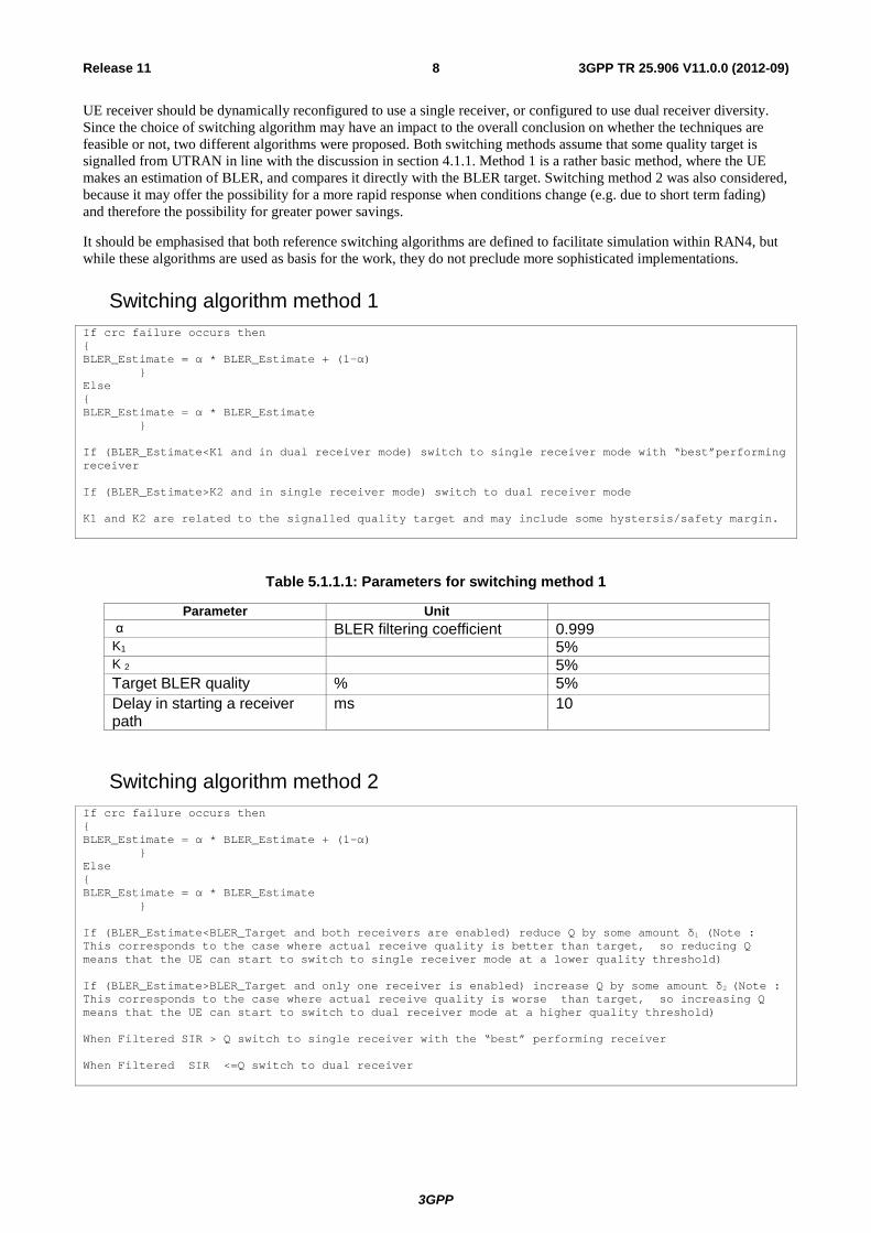
UE receiver should be dynamically reconfigured to use a single receiver, or configured to use dual receiver diversity. Since the choice of switching algorithm may have an impact to the overall conclusion on whether the techniques are feasible or not, two different algorithms were proposed. Both switching methods assume that some quality target is signalled from UTRAN in line with the discussion in section 4.1.1. Method 1 is a rather basic method, where the UE makes an estimation of BLER, and compares it directly with the BLER target. Switching method 2 was also considered, because it may offer the possibility for a more rapid response when conditions change (e.g. due to short term fading) and therefore the possibility for greater power savings.

It should be emphasised that both reference switching algorithms are defined to facilitate simulation within RAN4, but while these algorithms are used as basis for the work, they do not preclude more sophisticated implementations.

Switching algorithm method 1 If crc failure occurs then { BLER_Estimate = α * BLER_Estimate + (1-α) } Else { BLER_Estimate = α * BLER_Estimate } If (BLER_Estimate<K1 and in dual receiver mode) switch to single receiver mode with “best”performing receiver If (BLER_Estimate>K2 and in single receiver mode) switch to dual receiver mode K1 and K2 are related to the signalled quality target and may include some hystersis/safety margin.

Table 5.1.1.1: Parameters for switching method 1

Parameter Unit α BLER filtering coefficient 0.999 K1 5% K 2 5% Target BLER quality % 5% Delay in starting a receiver path

ms 10

Switching algorithm method 2 If crc failure occurs then { BLER_Estimate = α * BLER_Estimate + (1-α) } Else { BLER_Estimate = α * BLER_Estimate } If (BLER_Estimate<BLER_Target and both receivers are enabled) reduce Q by some amount δ1 (Note : This corresponds to the case where actual receive quality is better than target, so reducing Q means that the UE can start to switch to single receiver mode at a lower quality threshold) If (BLER_Estimate>BLER_Target and only one receiver is enabled) increase Q by some amount δ2 (Note : This corresponds to the case where actual receive quality is worse than target, so increasing Q means that the UE can start to switch to dual receiver mode at a higher quality threshold) When Filtered SIR > Q switch to single receiver with the “best” performing receiver When Filtered SIR <=Q switch to dual receiver

3GPP

3GPP TR 25.906 V11.0.0 (2012-09)9Release 11

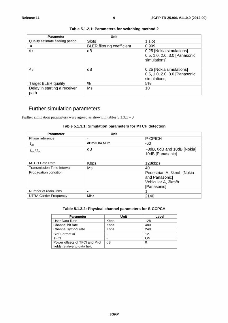
Table 5.1.2.1: Parameters for switching method 2

Parameter Unit Quality estimate filtering period Slots 1 slot α BLER filtering coefficient 0.999 δ 1 dB 0.25 [Nokia simulations]

0.5, 1.0, 2.0, 3.0 [Panasonic simulations]

δ 2 dB 0.25 [Nokia simulations] 0.5, 1.0, 2.0, 3.0 [Panasonic simulations]

Target BLER quality % 5% Delay in starting a receiver path

Ms 10

Further simulation parameters Further simulation parameters were agreed as shown in tables 5.1.3.1 – 3

Table 5.1.3.1: Simulation parameters for MTCH detection

Parameter Unit Phase reference - P-CPICH

ocI dBm/3.84 MHz -60

ocor II dB -3dB, 0dB and 10dB [Nokia] 10dB [Panasonic]

MTCH Data Rate Kbps 128kbps Transmission Time Interval Ms 40 Propagation condition Pedestrian A, 3km/h [Nokia

and Panasonic] Vehicular A, 3km/h [Panasonic]

Number of radio links - 1 UTRA Carrier Frequency MHz 2140

Table 5.1.3.2: Physical channel parameters for S-CCPCH

Parameter Unit Level User Data Rate Kbps 128 Channel bit rate Kbps 480 Channel symbol rate Kbps 240 Slot Format #i - 12 TFCI - ON Power offsets of TFCI and Pilot fields relative to data field

dB 0

3GPP

3GPP TR 25.906 V11.0.0 (2012-09)10Release 11

Table 5.1.3.3: Transport channel parameters for S-CCPCH

Parameter MTCH User Data Rate 128 kbps

40 ms TTI Transport Channel Number 1 Transport Block Size 2560 Transport Block Set Size 5120 Nr of transport blocks/TTI 2 RLC SDU block size 5072 Transmission Time Interval 40 ms Type of Error Protection Turbo Rate Matching attribute 256 Size of CRC 16 Position of TrCH in radio frame Flexible

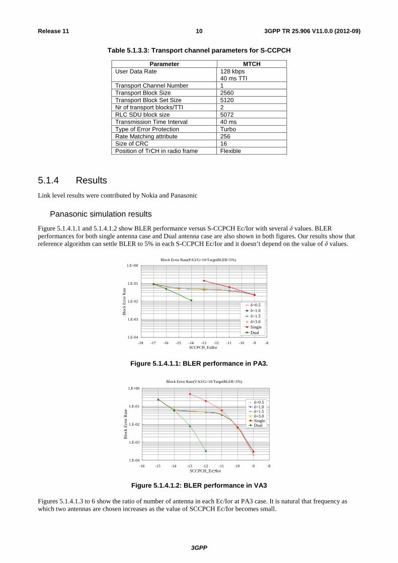
5.1.4 Results Link level results were contributed by Nokia and Panasonic

Panasonic simulation results

Figure 5.1.4.1.1 and 5.1.4.1.2 show BLER performance versus S-CCPCH Ec/Ior with several δ values. BLER performances for both single antenna case and Dual antenna case are also shown in both figures. Our results show that reference algorithm can settle BLER to 5% in each S-CCPCH Ec/Ior and it doesn’t depend on the value of δ values.

Block Error Rate(PA3/G=10/TargetBLER=5%)

1.E-04

1.E-03

1.E-02

1.E-01

1.E+00

-18 -17 -16 -15 -14 -13 -12 -11 -10 -9 -8SCCPCH_Eｃ/Ior

Blo

ck E

rror

Rat

e

δ=0.5δ=1.0δ=1.5δ=3.0SingleDual

Figure 5.1.4.1.1: BLER performance in PA3.

Block Error Rate(VA3/G=10/TargetBLER=5%)

1.E-04

1.E-03

1.E-02

1.E-01

1.E+00

-16 -15 -14 -13 -12 -11 -10 -9 -8SCCPCH_Eｃ・Ior

Blo

ck E

rror

Rat

e

δ=0.5δ=1.0δ=1.5δ=3.0SingleDual

Figure 5.1.4.1.2: BLER performance in VA3

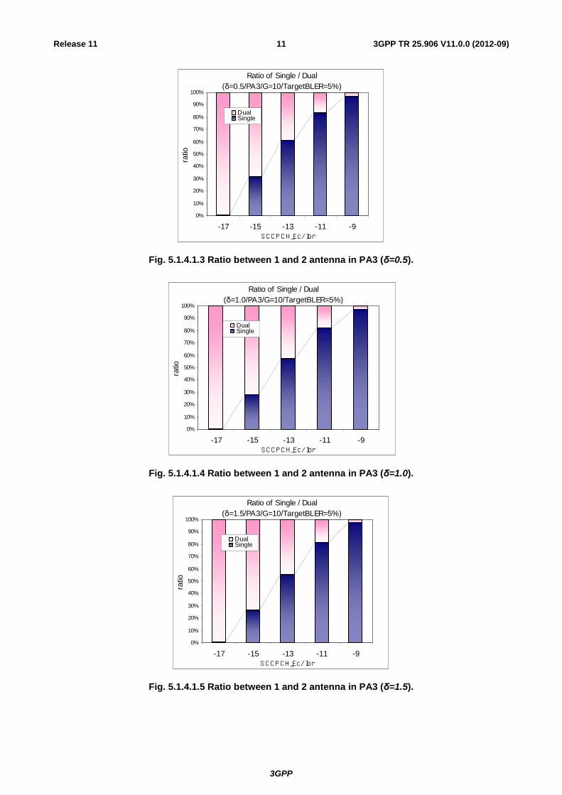
Figures 5.1.4.1.3 to 6 show the ratio of number of antenna in each Ec/Ior at PA3 case. It is natural that frequency as which two antennas are chosen increases as the value of SCCPCH Ec/Ior becomes small.

3GPP

3GPP TR 25.906 V11.0.0 (2012-09)11Release 11

Ratio of Single / Dual(δ=0.5/PA3/G=10/TargetBLER=5%)

0%

10%

20%

30%

40%

50%

60%

70%

80%

90%

100%

-17 -15 -13 -11 -9SCCPCH_Ec/Ior

ratio

DualSingle

Fig. 5.1.4.1.3 Ratio between 1 and 2 antenna in PA3 (δ=0.5).

Ratio of Single / Dual(δ=1.0/PA3/G=10/TargetBLER=5%)

0%

10%

20%

30%

40%

50%

60%

70%

80%

90%

100%

-17 -15 -13 -11 -9SCCPCH_Ec/Ior

ratio

DualSingle

Fig. 5.1.4.1.4 Ratio between 1 and 2 antenna in PA3 (δ=1.0).

Ratio of Single / Dual(δ=1.5/PA3/G=10/TargetBLER=5%)

0%

10%

20%

30%

40%

50%

60%

70%

80%

90%

100%

-17 -15 -13 -11 -9SCCPCH_Ec/Ior

ratio

DualSingle

Fig. 5.1.4.1.5 Ratio between 1 and 2 antenna in PA3 (δ=1.5).

3GPP

3GPP TR 25.906 V11.0.0 (2012-09)12Release 11

Ratio of Single / Dual(δ=3.0/PA3/G=10/TargetBLER=5%)

0%

10%

20%

30%

40%

50%

60%

70%

80%

90%

100%

-17 -15 -13 -11 -9SCCPCH_Ec/Ior

ratio

DualSingle

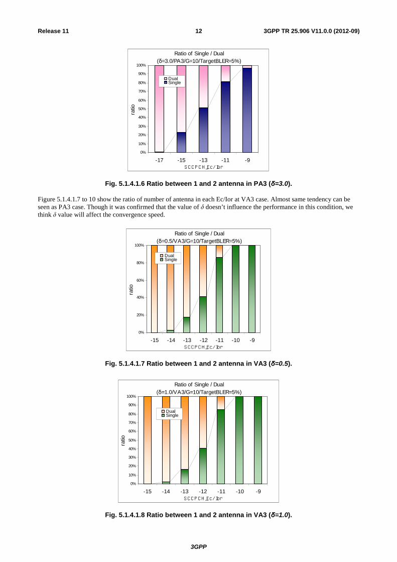
Fig. 5.1.4.1.6 Ratio between 1 and 2 antenna in PA3 (δ=3.0).

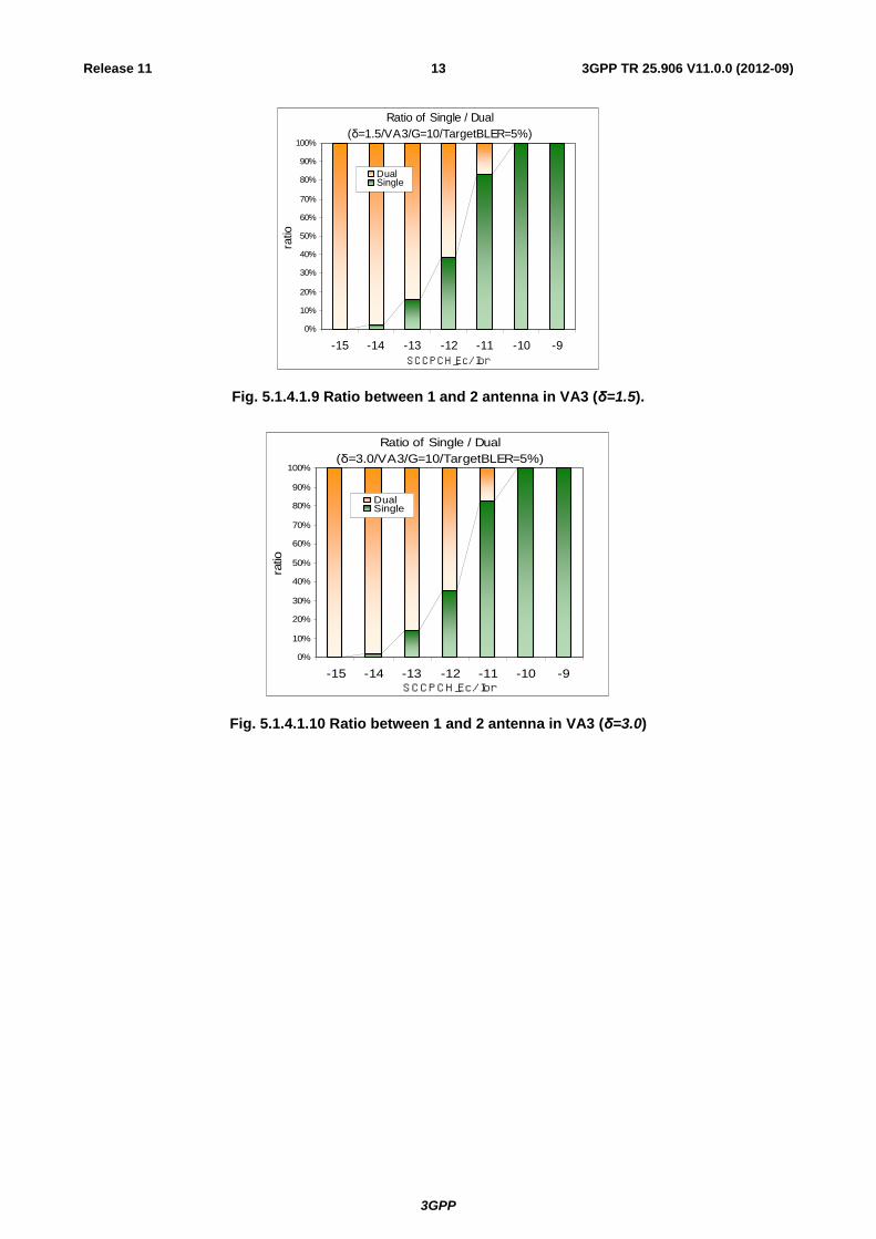
Figure 5.1.4.1.7 to 10 show the ratio of number of antenna in each Ec/Ior at VA3 case. Almost same tendency can be seen as PA3 case. Though it was confirmed that the value of δ doesn’t influence the performance in this condition, we think δ value will affect the convergence speed.

Ratio of Single / Dual(δ=0.5/VA3/G=10/TargetBLER=5%)

0%

20%

40%

60%

80%

100%

-15 -14 -13 -12 -11 -10 -9SCCPCH_Ec/Ior

ratio

DualSingle

Fig. 5.1.4.1.7 Ratio between 1 and 2 antenna in VA3 (δ=0.5).

Ratio of Single / Dual(δ=1.0/VA3/G=10/TargetBLER=5%)

0%

10%

20%

30%

40%

50%

60%

70%

80%

90%

100%

-15 -14 -13 -12 -11 -10 -9SCCPCH_Ec/Ior

ratio

DualSingle

Fig. 5.1.4.1.8 Ratio between 1 and 2 antenna in VA3 (δ=1.0).

3GPP

3GPP TR 25.906 V11.0.0 (2012-09)13Release 11

Ratio of Single / Dual(δ=1.5/VA3/G=10/TargetBLER=5%)

0%

10%

20%

30%

40%

50%

60%

70%

80%

90%

100%

-15 -14 -13 -12 -11 -10 -9SCCPCH_Ec/Ior

ratio

DualSingle

Fig. 5.1.4.1.9 Ratio between 1 and 2 antenna in VA3 (δ=1.5).

Ratio of Single / Dual(δ=3.0/VA3/G=10/TargetBLER=5%)

0%

10%

20%

30%

40%

50%

60%

70%

80%

90%

100%

-15 -14 -13 -12 -11 -10 -9SCCPCH_Ec/Ior

ratio

DualSingle

Fig. 5.1.4.1.10 Ratio between 1 and 2 antenna in VA3 (δ=3.0)

3GPP

3GPP TR 25.906 V11.0.0 (2012-09)14Release 11

Nokia simulation results

G=-3dB

0.0001

0.001

0.01

0.1

1-16 -14 -12 -10 -8 -6 -4 -2 0

SCCPCH Ec/Ior

BLE

R

1RX2RXSwitched - Method 1Switched - Method 2Quality Target

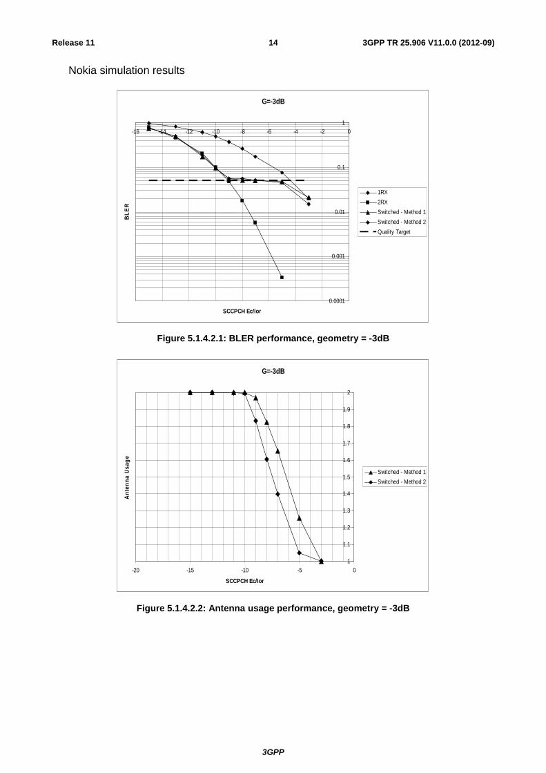
Figure 5.1.4.2.1: BLER performance, geometry = -3dB

G=-3dB

1

1.1

1.2

1.3

1.4

1.5

1.6

1.7

1.8

1.9

2

-20 -15 -10 -5 0

SCCPCH Ec/Ior

Ante

nna

Usa

ge

Switched - Method 1Switched - Method 2

Figure 5.1.4.2.2: Antenna usage performance, geometry = -3dB

3GPP

3GPP TR 25.906 V11.0.0 (2012-09)15Release 11

G=0dB

0.0001

0.001

0.01

0.1

1-20 -18 -16 -14 -12 -10 -8 -6 -4 -2 0

SCCPCH Ec/Ior

BLER

1RX2RXSwitched - Method 1Switched - Method 2Quality Target

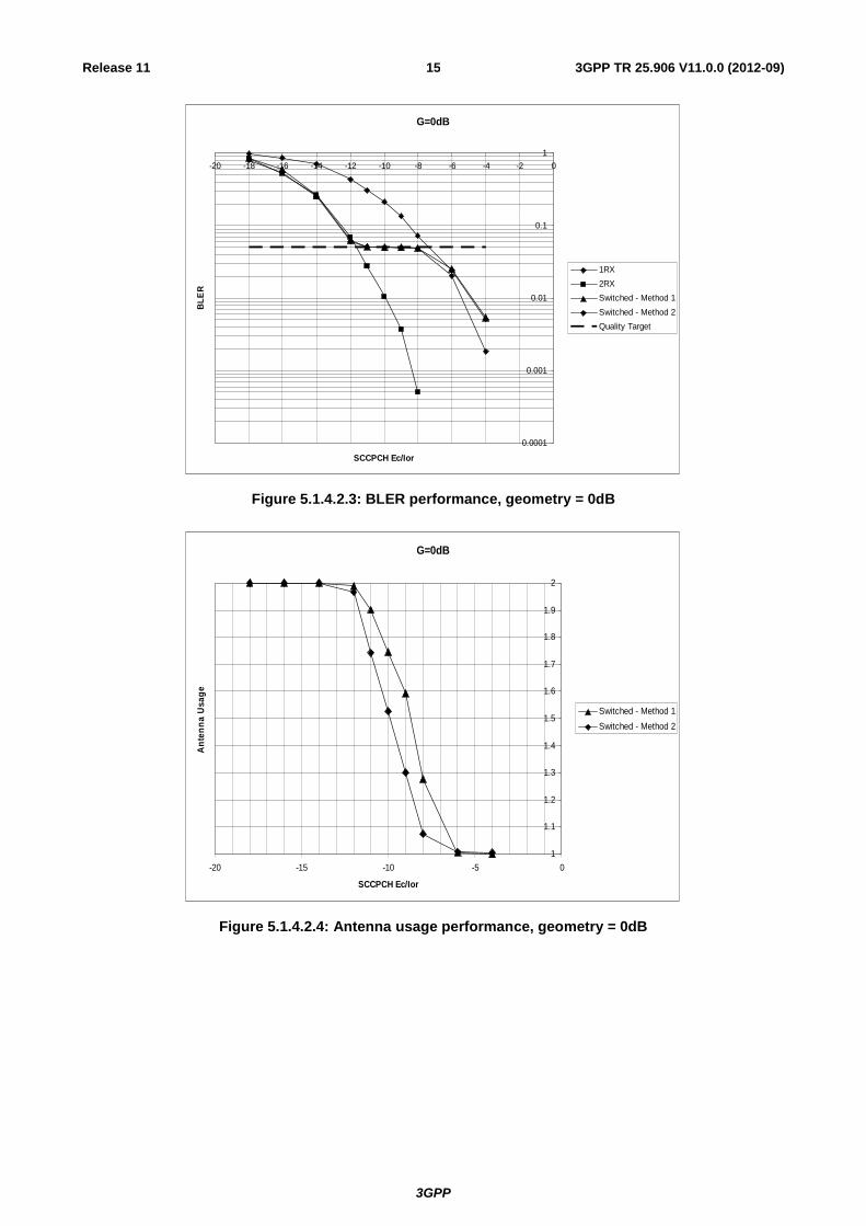
Figure 5.1.4.2.3: BLER performance, geometry = 0dB

G=0dB

1

1.1

1.2

1.3

1.4

1.5

1.6

1.7

1.8

1.9

2

-20 -15 -10 -5 0

SCCPCH Ec/Ior

Ante

nna

Usa

ge

Switched - Method 1Switched - Method 2

Figure 5.1.4.2.4: Antenna usage performance, geometry = 0dB

3GPP

3GPP TR 25.906 V11.0.0 (2012-09)16Release 11

G=10dB

0.001

0.01

0.1

1-30 -28 -26 -24 -22 -20 -18 -16 -14 -12 -10

SCCPCH Ec/Ior

BLE

R

1RX2RXSwitched - Method 1Switched - Method 2Quality Target

b4

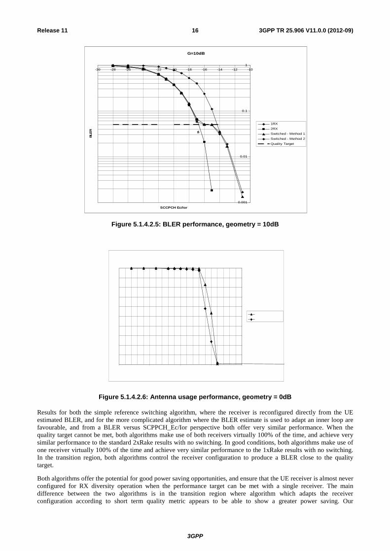
Figure 5.1.4.2.5: BLER performance, geometry = 10dB

Figure 5.1.4.2.6: Antenna usage performance, geometry = 0dB

Results for both the simple reference switching algorithm, where the receiver is reconfigured directly from the UE estimated BLER, and for the more complicated algorithm where the BLER estimate is used to adapt an inner loop are favourable, and from a BLER versus SCPPCH_Ec/Ior perspective both offer very similar performance. When the quality target cannot be met, both algorithms make use of both receivers virtually 100% of the time, and achieve very similar performance to the standard 2xRake results with no switching. In good conditions, both algorithms make use of one receiver virtually 100% of the time and achieve very similar performance to the 1xRake results with no switching. In the transition region, both algorithms control the receiver configuration to produce a BLER close to the quality target.

Both algorithms offer the potential for good power saving opportunities, and ensure that the UE receiver is almost never configured for RX diversity operation when the performance target can be met with a single receiver. The main difference between the two algorithms is in the transition region where algorithm which adapts the receiver configuration according to short term quality metric appears to be able to show a greater power saving. Our

3GPP

3GPP TR 25.906 V11.0.0 (2012-09)17Release 11

understanding is that this happens because it is able to respond opportunistically to changes in channel conditions due to short term fading.

Based on these results, the indication is that dynamic receiver reconfiguration is a feasible technique when receiving p-t-m MBMS transmissions. Provided that a suitable quality target can be provided to the UE, the technique appears to offer the possibility for power saving opportunities without compromising the performance of the 2RX when conditions are demanding.

6 MBMS system level simulation scenarios, assumptions and results

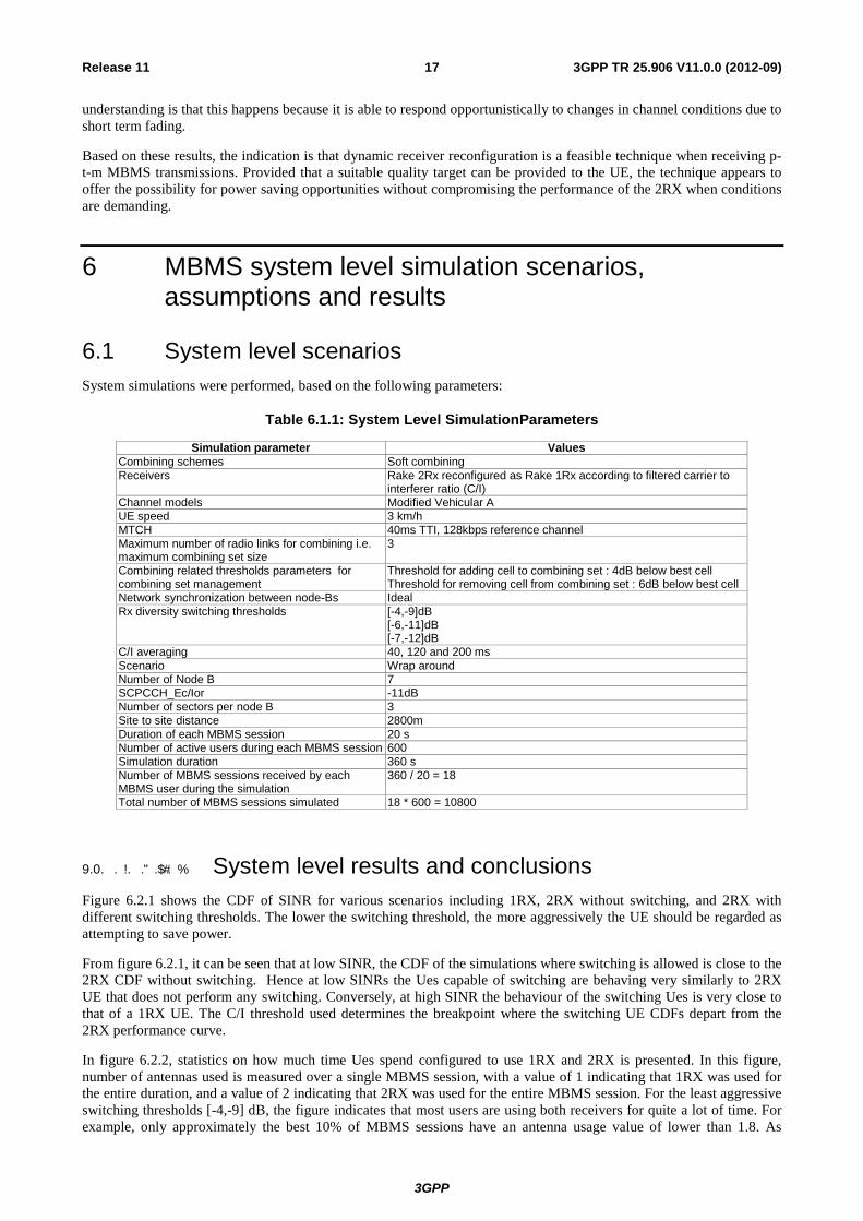
6.1 System level scenarios System simulations were performed, based on the following parameters:

Table 6.1.1: System Level SimulationParameters

Simulation parameter Values Combining schemes Soft combining Receivers Rake 2Rx reconfigured as Rake 1Rx according to filtered carrier to

interferer ratio (C/I) Channel models Modified Vehicular A UE speed 3 km/h MTCH 40ms TTI, 128kbps reference channel Maximum number of radio links for combining i.e. maximum combining set size

3

Combining related thresholds parameters for combining set management

Threshold for adding cell to combining set : 4dB below best cell Threshold for removing cell from combining set : 6dB below best cell

Network synchronization between node-Bs Ideal Rx diversity switching thresholds [-4,-9]dB

[-6,-11]dB [-7,-12]dB

C/I averaging 40, 120 and 200 ms Scenario Wrap around Number of Node B 7 SCPCCH_Ec/Ior -11dB Number of sectors per node B 3 Site to site distance 2800m Duration of each MBMS session 20 s Number of active users during each MBMS session 600 Simulation duration 360 s Number of MBMS sessions received by each MBMS user during the simulation

360 / 20 = 18

Total number of MBMS sessions simulated 18 * 600 = 10800

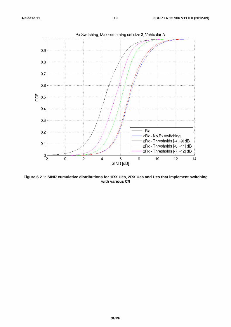
� � � �9.0. . . . .� �. System level results and conclusions Figure 6.2.1 shows the CDF of SINR for various scenarios including 1RX, 2RX without switching, and 2RX with different switching thresholds. The lower the switching threshold, the more aggressively the UE should be regarded as attempting to save power.

From figure 6.2.1, it can be seen that at low SINR, the CDF of the simulations where switching is allowed is close to the 2RX CDF without switching. Hence at low SINRs the Ues capable of switching are behaving very similarly to 2RX UE that does not perform any switching. Conversely, at high SINR the behaviour of the switching Ues is very close to that of a 1RX UE. The C/I threshold used determines the breakpoint where the switching UE CDFs depart from the 2RX performance curve.

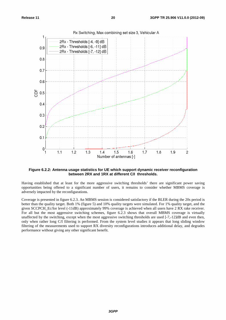
In figure 6.2.2, statistics on how much time Ues spend configured to use 1RX and 2RX is presented. In this figure, number of antennas used is measured over a single MBMS session, with a value of 1 indicating that 1RX was used for the entire duration, and a value of 2 indicating that 2RX was used for the entire MBMS session. For the least aggressive switching thresholds [-4,-9] dB, the figure indicates that most users are using both receivers for quite a lot of time. For example, only approximately the best 10% of MBMS sessions have an antenna usage value of lower than 1.8. As

3GPP

3GPP TR 25.906 V11.0.0 (2012-09)18Release 11

expected, more sessions are performed with lower antenna usage when more aggressive thresholds are taken into use, and for the most aggressive threshold corresponding to [-7,-12] dB some 50% of MBMS sessions have an antenna usage figure of less than 1.2. This indicates that for this threshold, a significant proportion (e.g. 50%) of the MBMS users would be expected to be experiencing worthwhile power saving. Indeed some 20% of MBMS sessions are performed with only one antenna used.

3GPP

3GPP TR 25.906 V11.0.0 (2012-09)19Release 11

Figure 6.2.1: SINR cumulative distributions for 1RX Ues, 2RX Ues and Ues that implement switching with various C/I

3GPP

3GPP TR 25.906 V11.0.0 (2012-09)20Release 11

Figure 6.2.2: Antenna usage statistics for UE which support dynamic receiver reconfiguration between 2RX and 1RX at different C/I thresholds.

Having established that at least for the more aggressive switching thresholds’ there are significant power saving opportunities being offered to a significant number of users, it remains to consider whether MBMS coverage is adversely impacted by the reconfigurations.

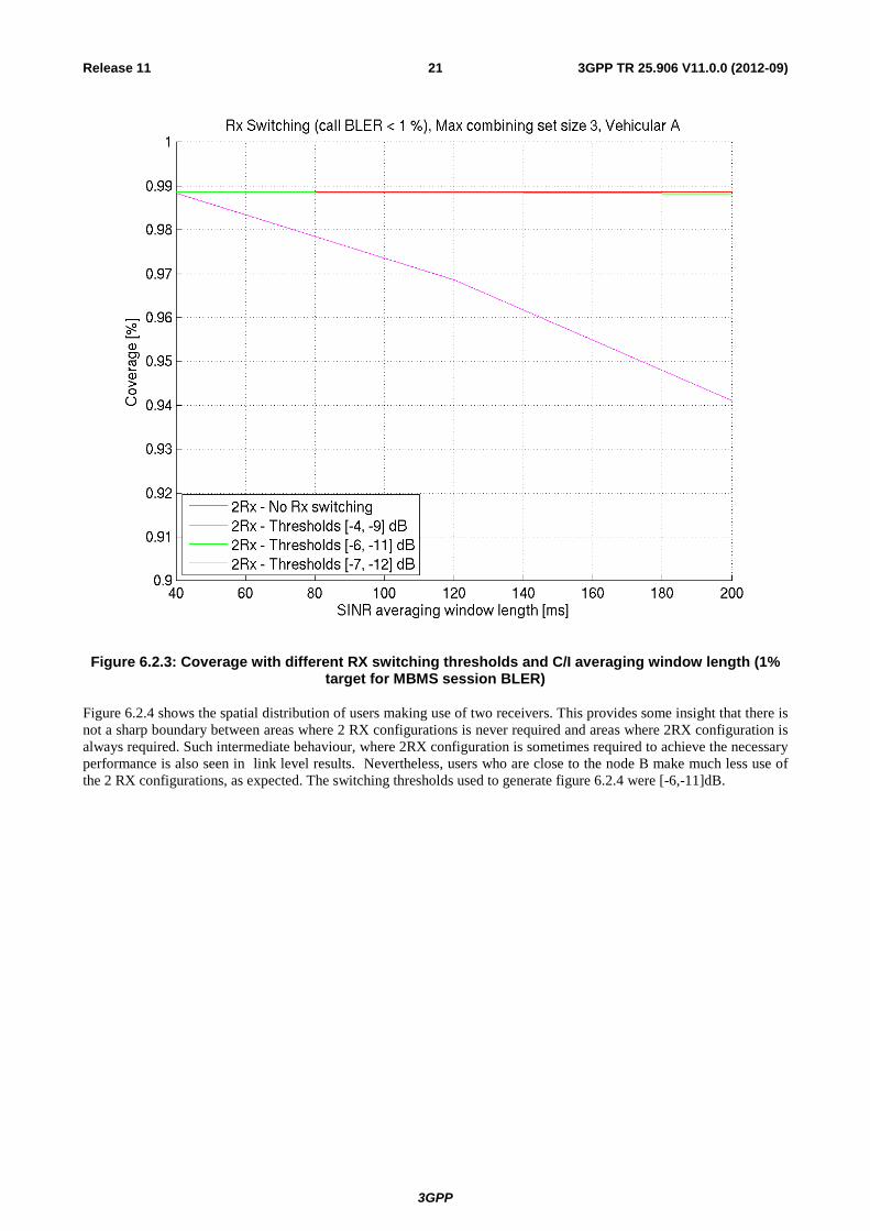
Coverage is presented in figure 6.2.3. An MBMS session is considered satisfactory if the BLER during the 20s period is better than the quality target. Both 1% (figure 5) and 10% quality targets were simulated. For 1% quality target, and the given SCCPCH_Ec/Ior level (-11dB) approximately 99% coverage is achieved when all users have 2 RX rake receiver. For all but the most aggressive switching schemes, figure 6.2.3 shows that overall MBMS coverage is virtually unaffected by the switching, except when the most aggressive switching thresholds are used [-7,-12]dB and even then, only when rather long C/I filtering is performed. From the system level studies it appears that long sliding window filtering of the measurements used to support RX diversity reconfigurations introduces additional delay, and degrades performance without giving any other significant benefit.

3GPP

3GPP TR 25.906 V11.0.0 (2012-09)21Release 11

Figure 6.2.3: Coverage with different RX switching thresholds and C/I averaging window length (1% target for MBMS session BLER)

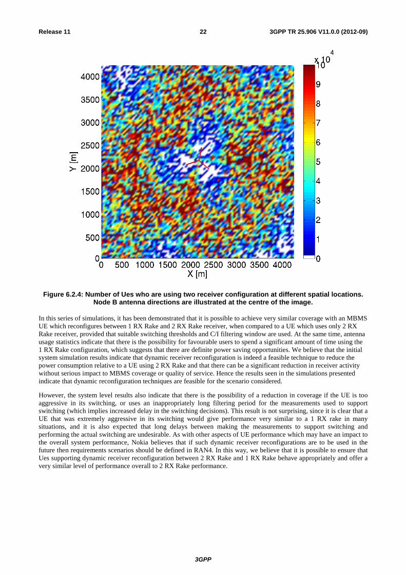
Figure 6.2.4 shows the spatial distribution of users making use of two receivers. This provides some insight that there is not a sharp boundary between areas where 2 RX configurations is never required and areas where 2RX configuration is always required. Such intermediate behaviour, where 2RX configuration is sometimes required to achieve the necessary performance is also seen in link level results. Nevertheless, users who are close to the node B make much less use of the 2 RX configurations, as expected. The switching thresholds used to generate figure 6.2.4 were [-6,-11]dB.

3GPP

3GPP TR 25.906 V11.0.0 (2012-09)22Release 11

Figure 6.2.4: Number of Ues who are using two receiver configuration at different spatial locations. Node B antenna directions are illustrated at the centre of the image.

In this series of simulations, it has been demonstrated that it is possible to achieve very similar coverage with an MBMS UE which reconfigures between 1 RX Rake and 2 RX Rake receiver, when compared to a UE which uses only 2 RX Rake receiver, provided that suitable switching thresholds and C/I filtering window are used. At the same time, antenna usage statistics indicate that there is the possibility for favourable users to spend a significant amount of time using the 1 RX Rake configuration, which suggests that there are definite power saving opportunities. We believe that the initial system simulation results indicate that dynamic receiver reconfiguration is indeed a feasible technique to reduce the power consumption relative to a UE using 2 RX Rake and that there can be a significant reduction in receiver activity without serious impact to MBMS coverage or quality of service. Hence the results seen in the simulations presented indicate that dynamic reconfiguration techniques are feasible for the scenario considered.

However, the system level results also indicate that there is the possibility of a reduction in coverage if the UE is too aggressive in its switching, or uses an inappropriately long filtering period for the measurements used to support switching (which implies increased delay in the switching decisions). This result is not surprising, since it is clear that a UE that was extremely aggressive in its switching would give performance very similar to a 1 RX rake in many situations, and it is also expected that long delays between making the measurements to support switching and performing the actual switching are undesirable. As with other aspects of UE performance which may have an impact to the overall system performance, Nokia believes that if such dynamic receiver reconfigurations are to be used in the future then requirements scenarios should be defined in RAN4. In this way, we believe that it is possible to ensure that Ues supporting dynamic receiver reconfiguration between 2 RX Rake and 1 RX Rake behave appropriately and offer a very similar level of performance overall to 2 RX Rake performance.

3GPP

3GPP TR 25.906 V11.0.0 (2012-09)23Release 11

7 Non-MBMS link level simulation scenarios, assumptions and result

7.0 General This section explores results of receive diversity (RxDiv) reconfiguration for DCH/F-DPCH and HSDPA downlink channels under certain conditions.

Switching algorithm methods are proposed for dedicated and HSDPA DL channels separately. It should be stressed that in order for the UE to turn off RxDiv, the conditions for doing so would need to be satisfied for all physical channels currently being received by the UE.

� � � �9.0. . . . .� �. Link level scenarios for dedicated channels When in a near-site scenario the base station (BS) will be rather likely at the lowest minimum output power because the dynamic power range of the BS (typical values are 30 dB) may be smaller than the path loss dynamic range (typical values are 70 dB). In this scenario, the downlink transmitted power is not further reduced due to the use of a RxDiv receiver at the UE and thus the RxDiv receiver can be switched off. Furthermore, this scenario can be detected since the average measured SIR remains above the target SIR when the transmitter reaches the minimum power limit.

An algorithm for the RxDiv switching that was simulated is described in the following sub-section.

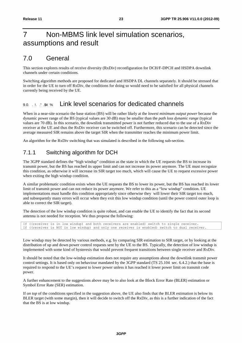
7.1.1 Switching algorithm for DCH The 3GPP standard defines the “high windup” condition as the state in which the UE requests the BS to increase its transmit power, but the BS has reached its upper limit and can not increase its power anymore. The UE must recognize this condition, as otherwise it will increase its SIR target too much, which will cause the UE to request excessive power when exiting the high windup condition.

A similar problematic condition exists when the UE requests the BS to lower its power, but the BS has reached its lower limit of transmit power and can not reduce its power anymore. We refer to this as a “low windup” condition. UE implementations must handle this condition appropriately since otherwise they will lower their SIR target too much, and subsequently many errors will occur when they exit this low windup condition (until the power control outer loop is able to correct the SIR target).

The detection of the low windup condition is quite robust, and can enable the UE to identify the fact that its second antenna is not needed for reception. We thus propose the following:

If ((receiver is in low windup) and both receivers are enabled) switch to single receiver. If ((receiver is NOT in low windup) and only one receiver is enabled) switch to dual receiver.

Low windup may be detected by various methods, e.g. by comparing SIR estimation to SIR target, or by looking at the distribution of up and down power control requests sent by the UE to the BS. Typically, the detection of low windup is implemented with some kind of hysteresis that would prevent frequent transitions between single receiver and RxDiv.

It should be noted that the low-windup estimation does not require any assumptions about the downlink transmit power control settings. It is based only on behaviour mandated by the 3GPP standard (TS 25.104 sec. 6.4.2.) that the base is required to respond to the UE’s request to lower power unless it has reached it lower power limit on transmit code power.

A further enhancement to the suggestions above may be to also look at the Block Error Rate (BLER) estimation or Symbol Error Rate (SER) estimation.

If on top of the conditions specified in the suggestion above, the UE also finds that the BLER estimation is below its BLER target (with some margin), then it will decide to switch off the RxDiv, as this is a further indication of the fact that the BS is at low windup.

3GPP

3GPP TR 25.906 V11.0.0 (2012-09)24Release 11

This enhancement can help in test cases in which the BS does not perform power control, since in the test case the BS will signal to the UE a very low BLER target (which will not be met in the test), and thus the UE will not switch off RxDiv and will maintain the required performance for RxDiv receivers.

In channels such as Fractional DCH (FDCH) where a BLER target is replaced by TPC command ER target (equivalent to Symbol Error Rate, SER), the same principal can be maintained with SER estimation versus SER target.

It is important to note, that when a UE is even near the condition of low windup, the potential BS power savings that can be achieved by utilizing RxDiv at the UE is minimal, since the transmitted BS power is so low anyway. Thus the possibility that erroneously switching off RxDiv under such conditions will degrade system capacity is negligible.

Simulation conditions

Table 7.1.2.1: DCH Simulation conditions

Parameter Unit Receiver Type - Type 1 Channel Estimation - ON; everything else is IDEAL receiver

ocor II dB Switch between -3 and 10

ocI dBm/3.84 MHz -60

Information Data Rate kbps 12.2 Target quality value on DTCH BLER 0.01 Target quality value on DCCH BLER - Propagation condition STATIC and CASE1 Maximum_DL_Power * dB 7 Minimum_DL_Power * dB -18 DL Power Control step size, DTPC dB 1 Limited Power Increase - “Not used” Low-Windup Identification - Estimated Switch to single antenna - Choosing the antenna with better reception

7.1.3 Simulation results Link level simulation results were contributed by Marvell for STATIC and CASE1 propagation channels.

Static channel conditions

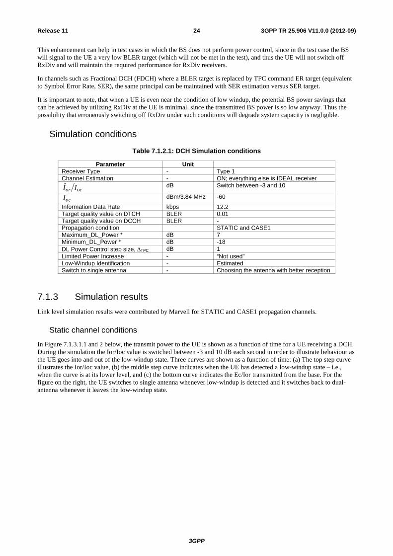
In Figure 7.1.3.1.1 and 2 below, the transmit power to the UE is shown as a function of time for a UE receiving a DCH. During the simulation the Ior/Ioc value is switched between -3 and 10 dB each second in order to illustrate behaviour as the UE goes into and out of the low-windup state. Three curves are shown as a function of time: (a) The top step curve illustrates the Ior/Ioc value, (b) the middle step curve indicates when the UE has detected a low-windup state – i.e., when the curve is at its lower level, and (c) the bottom curve indicates the Ec/Ior transmitted from the base. For the figure on the right, the UE switches to single antenna whenever low-windup is detected and it switches back to dual-antenna whenever it leaves the low-windup state.

3GPP

3GPP TR 25.906 V11.0.0 (2012-09)25Release 11

0 1 2 3 4 5 6 7-30

-25

-20

-15

-10

-5

0

5

10

15

time (sec)

AWGN - UE always uses 2 Antenna

Ior/Ioc[dB]Ec/Ior[dB]

WindUp

0 1 2 3 4 5 6 7-30

-25

-20

-15

-10

-5

0

5

10

15

time (sec)

AWGN - UE switchs 2nd Antenna by Low Windup

Ior/Ioc[dB]Ec/Ior[dB]

WindUp

*Figure 7.1.3.1.1 and 2: Static channel simulation results for DCH reception

It can be seen from these figures that very little additional downlink power is needed to support the UE that does antenna dynamic reconfiguration. Averaging over the simulations showed an increase of average Ec/Ior from -27.94 dB (0.161%) to -27.48 dB (0.179%) when switching off the second antenna, corresponding to an increase of 0.018% in base transmit power.

Case1 channel conditions

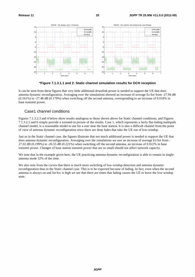
Figures 7.1.3.2.3 and 4 below show results analogous to those shown above for Static channel conditions, and Figures 7.1.3.2.5 and 6 simply provide a zoomed-in picture of the results. Case 1, which represents a fairly flat-fading multipath channel model, is a reasonable model to use for a user near the base station. It is also a difficult channel from the point of view of antenna dynamic reconfiguration since there are deep fades that take the UE out of low-windup.

Just as in the Static channel case, the figures illustrate that not much additional power is needed to support the UE that does antenna dynamic reconfiguration. Averaging over the simulations we saw an increase of average Ec/Ior from -27.02 dB (0.199%) to -26.55 dB (0.221%) when switching off the second antenna, an increase of 0.022% in base transmit power. Changes of base station transmit power that are so small should not affect network capacity.

We note that in the example given here, the UE practicing antenna dynamic reconfiguration is able to remain in single-antenna mode 52% of the time.

We also note from the curves that there is much more switching of low-windup detection and antenna dynamic reconfiguration than in the Static channel case. This is to be expected because of fading. In fact, even when the second antenna is always on and Ior/Ioc is high we see that there are times that fading causes the UE to leave the low-windup state.

3GPP

3GPP TR 25.906 V11.0.0 (2012-09)26Release 11

0 1 2 3 4 5 6 7-30

-25

-20

-15

-10

-5

0

5

10

15

time (sec)

Case1 - UE switchs Best by Low Windup

Ior/Ioc[dB]Ec/Ior[dB]

WindUp

0 1 2 3 4 5 6 7-30

-25

-20

-15

-10

-5

0

5

10

15

time (sec)

Case1 - UE always uses 2 Antenna

Ior/Ioc[dB]Ec/Ior[dB]WindUp

2.2 2.4 2.6 2.8 3 3.2 3.4-30

-25

-20

-15

-10

-5

0

5

time (sec)

Case1 - UE switchs Best by Low Windup

Ior/Ioc[dB]Ec/Ior[dB]WindUp

2.2 2.4 2.6 2.8 3 3.2 3.4-30

-25

-20

-15

-10

-5

0

5

time (sec)

Case1 - UE always uses 2 Antenna

Ior/Ioc[dB]Ec/Ior[dB]WindUp

Figures 7.1.3.2.3 and 4: Case1 channel simulation results for DCH reception – zoomed in

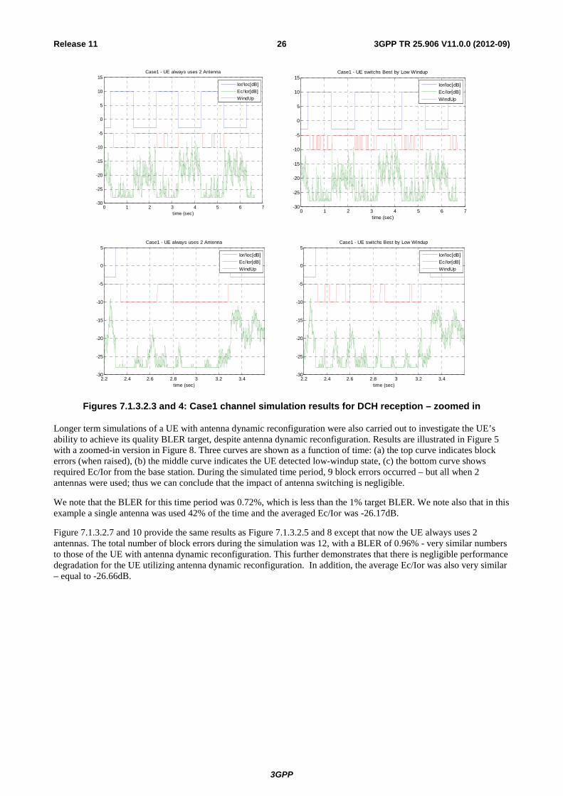
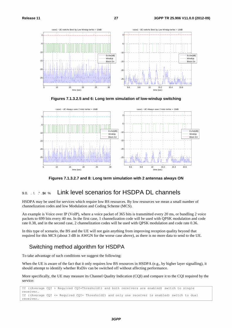
Longer term simulations of a UE with antenna dynamic reconfiguration were also carried out to investigate the UE’s ability to achieve its quality BLER target, despite antenna dynamic reconfiguration. Results are illustrated in Figure 5 with a zoomed-in version in Figure 8. Three curves are shown as a function of time: (a) the top curve indicates block errors (when raised), (b) the middle curve indicates the UE detected low-windup state, (c) the bottom curve shows required Ec/Ior from the base station. During the simulated time period, 9 block errors occurred – but all when 2 antennas were used; thus we can conclude that the impact of antenna switching is negligible.

We note that the BLER for this time period was 0.72%, which is less than the 1% target BLER. We note also that in this example a single antenna was used 42% of the time and the averaged Ec/Ior was -26.17dB.

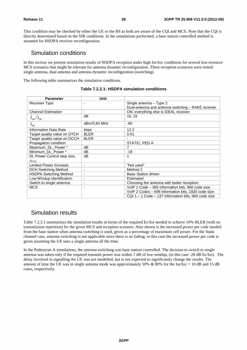
Figure 7.1.3.2.7 and 10 provide the same results as Figure 7.1.3.2.5 and 8 except that now the UE always uses 2 antennas. The total number of block errors during the simulation was 12, with a BLER of 0.96% - very similar numbers to those of the UE with antenna dynamic reconfiguration. This further demonstrates that there is negligible performance degradation for the UE utilizing antenna dynamic reconfiguration. In addition, the average Ec/Ior was also very similar – equal to -26.66dB.

3GPP

3GPP TR 25.906 V11.0.0 (2012-09)27Release 11

9.6 9.8 10 10.2 10.4 10.6

-25

-20

-15

-10

-5

0

time (sec)

case1 - UE switchs Best by Low Windup Ior/Ioc = 10dB

Ec/Ior[dB]WindUpBlock Err

5 10 15 20 25 30

-25

-20

-15

-10

-5

0

time (sec)

case1 - UE switchs Best by Low Windup Ior/Ioc = 10dB

Ec/Ior[dB]WindUpBlock Err

Figures 7.1.3.2.5 and 6: Long term simulation of low-windup switching

5 10 15 20 25 30

-25

-20

-15

-10

-5

0

time (sec)

case1 - UE Always uses 2 Ants Ior/Ioc = 10dB

Ec/Ior[dB]WindUpBlock Err

9.6 9.8 10 10.2 10.4 10.6

-25

-20

-15

-10

-5

0

time (sec)

case1 - UE Always uses 2 Ants Ior/Ioc = 10dB

Ec/Ior[dB]WindUpBlock Err

Figures 7.1.3.2.7 and 8: Long term simulation with 2 antennas always ON

� � � �9.0. . . . .� �. Link level scenarios for HSDPA DL channels HSDPA may be used for services which require low BS resources. By low resources we mean a small number of channelization codes and low Modulation and Coding Scheme (MCS).

An example is Voice over IP (VoIP), where a voice packet of 365 bits is transmitted every 20 ms, or bundling 2 voice packets to 699 bits every 40 ms. In the first case, 1 channelization code will be used with QPSK modulation and code rate 0.38, and in the second case, 2 channelization codes will be used with QPSK modulation and code rate 0.36.

In this type of scenario, the BS and the UE will not gain anything from improving reception quality beyond that required for this MCS (about 3 dB in AWGN for the worse case above), as there is no more data to send to the UE.

Switching method algorithm for HSDPA To take advantage of such conditions we suggest the following:

When the UE is aware of the fact that it only requires low BS resources in HSDPA (e.g., by higher layer signalling), it should attempt to identify whether RxDiv can be switched off without affecting performance.

More specifically, the UE may measure its Channel Quality Indication (CQI) and compare it to the CQI required by the service:

If ((Average CQI > Required CQI+Threshold1) and both receivers are enabled) switch to single receiver. If ((Average CQI <= Required CQI+ Threshold2) and only one receiver is enabled) switch to dual receiver.

3GPP

3GPP TR 25.906 V11.0.0 (2012-09)28Release 11

This condition may be checked by either the UE or the BS as both are aware of the CQI and MCS. Note that the CQI is directly determined based on the SIR conditions. In the simulations performed, a base station controlled method is assumed for HSDPA receiver reconfiguration.

Simulation conditions In this section we present simulation results of HSDPA reception under high Ior/Ioc conditions for several low-resource MCS scenarios that might be relevant for antenna dynamic reconfiguration. Three reception scenarios were tested: single antenna, dual antenna and antenna dynamic reconfiguration (switching).

The following table summarizes the simulation conditions.

Table 7.2.2.1: HSDPA simulation conditions

Parameter Unit Receiver Type - Single antenna – Type 2

Dual-antenna and antenna switching – RAKE receiver Channel Estimation - ON; everything else is IDEAL receiver

ocor II dB 10, 15

ocI dBm/3.84 MHz -60

Information Data Rate kbps 12.2 Target quality value on DTCH BLER 0.01 Target quality value on DCCH BLER - Propagation condition STATIC, PED A Maximum_DL_Power * dB 7 Minimum_DL_Power * dB -18 DL Power Control step size, DTPC

dB 1

Limited Power Increase - “Not used” DCH Switching Method - Method 2 HSDPA Switching Method - Base Station driven Low-Windup Identification - Estimated Switch to single antenna - Choosing the antenna with better reception MCS - VoIP 1 Code – 365 information bits, 960 code size

VoIP 2 Codes – 699 information bits, 1920 code size CQI 1 – 1 Code – 137 information bits, 960 code size

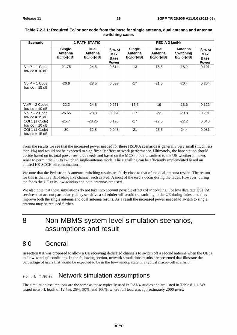
Simulation results Table 7.2.3.1 summarizes the simulation results in terms of the required Ec/Ior needed to achieve 10% BLER (with no transmission repetition) for the given MCS and reception scenario. Also shown is the increased power per code needed from the base station when antenna switching is used, given as a percentage of maximum cell power. For the Static channel case, antenna switching is not applicable since there is no fading; in this case the increased power per code is given assuming the UE uses a single antenna all the time.

In the Pedestrian A simulations, the antenna switching was base station controlled. The decision to switch to single antenna was taken only if the required transmit power was within 1 dB of low-windup, (in this case -28 dB Ec/Ior). The delay involved in signalling the UE was not modelled, but is not expected to significantly change the results. The amount of time the UE was in single antenna mode was approximately 50% & 80% for the Ior/Ioc = 10 dB and 15 dB cases, respectively.

3GPP

3GPP TR 25.906 V11.0.0 (2012-09)29Release 11

Table 7.2.3.1: Required Ec/Ior per code from the base for single antenna, dual antenna and antenna switching cases

Scenario 1 PATH STATIC PED A 3 km/Hr

Single Antenna

Ec/Ior[dB]

Dual Antenna

Ec/Ior[dB]

D% of Max Base

Power

Single Antenna

Ec/Ior[dB]

Dual Antenna

Ec/Ior[dB]

Antenna Switching Ec/Ior[dB]

D% of Max Base

Power VoIP – 1 Code Ior/Ioc = 10 dB

-21.75 -24.5 0.314 -13 -18.5 -18.2 0.101

VoIP – 1 Code Ior/Ioc = 15 dB

-26.6 -28.5 0.099 -17 -21.5 -20.4 0.204

VoIP – 2 Codes Ior/Ioc = 10 dB

-22.2 -24.8 0.271 -13.8 -19 -18.6 0.122

VoIP – 2 Code Ior/Ioc = 15 dB

-26.65 -28.8 0.084 -17 -22 -20.8 0.201

CQI 1 (1 Code) Ior/Ioc = 10 dB

-25.7 -28.25 0.120 -17 -22.5 -22.2 0.040

CQI 1 (1 Code) Ior/Ioc = 15 dB

-30 -32.8 0.048 -21 -25.5 -24.4 0.081

From the results we see that the increased power needed for these HSDPA scenarios is generally very small (much less than 1%) and would not be expected to significantly affect network performance. Ultimately, the base station should decide based on its total power resource needs and based on the MCS to be transmitted to the UE whether it makes sense to permit the UE to switch to single-antenna mode. The signalling can be efficiently implemented based on unused HS-SCCH bit combinations.

We note that the Pedestrian A antenna switching results are fairly close to that of the dual-antenna results. The reason for this is that in a flat-fading like channel such as Ped. A most of the errors occur during the fades. However, during the fades the UE exits low-windup and both antennas are used.

We also note that these simulations do not take into account possible effects of scheduling. For low data rate HSDPA services that are not particularly delay sensitive a scheduler will avoid transmitting to the UE during fades, and thus improve both the single antenna and dual antenna results. As a result the increased power needed to switch to single antenna may be reduced further.

8 Non-MBMS system level simulation scenarios, assumptions and result

8.0 General In section 0 it was proposed to allow a UE receiving dedicated channels to switch off a second antenna when the UE is in “low-windup” conditions. In the following section, network simulations results are presented that illustrate the percentage of users that would be expected to be in the low-windup state in a typical macro-cell scenario.

� � � �9.0. . . . .� �. Network simulation assumptions The simulation assumptions are the same as those typically used in RAN4 studies and are listed in Table 8.1.1. We tested network loads of 12.5%, 25%, 50%, and 100%, where full load was approximately 2000 users.

3GPP

3GPP TR 25.906 V11.0.0 (2012-09)30Release 11

Table 8.1.1: Network Simulation Assumptions

Parameter Value Simulation Type Snapshot Network Type Hexagonal grid – two rings – 19 bases (wrap around

technique used); BTS in the middle of cell User Distribution Random and uniform across the network Cell Radius 577 meters Number Sectors per Base 3 (3-sectored 65 degree antennas) Propagation Loss Loss = 128,15 + 37,6log10I dB; R = distance in Km (Macro-

cell model as defined in [10]) MCL (including antenna again)-macro-cell

70 dB

Antenna gain (including losses) 11 dBi at Base; (0 dBi at UE) Log-normal fade standard deviation 10 dB Non-orthogonality factor Case 1 channel # of snapshots > 10000 for speech #PC steps per snapshot > 150 Step size PC Perfect PC PC error 0 % Margin in respect with target C/I 0 dB Initial TX power Random initial Outage condition Eb/N0 target not reached due to lack of TX power Satisfied user Measured Eb/N0 higher than Eb/N0 target – 0,5 dB Handover threshold for candidate set 3 dB Maximum number in active set 3 Choice of cells in the active step Random Combining Maximum ratio combining Noise figure 9 dB Receiving bandwidth 3,84 MHz Noise power -99 dBm Maximum BTS power 43 dBm Common Channel power CPICH_Ec/Ior = -10 dB

PCCPCH_Ec/Ior = -12 dB SCH_Ec/Ior = -12 dB PICH_Ec/Ior = -15 dB

Power control dynamic range 25 dB Data Rates 12,2 (voice), Activity factor 100% Maximum TX power for 12,2 kbps 30 dBm Eb/No target for 12,2 kbps 9 dB @ 1% FER

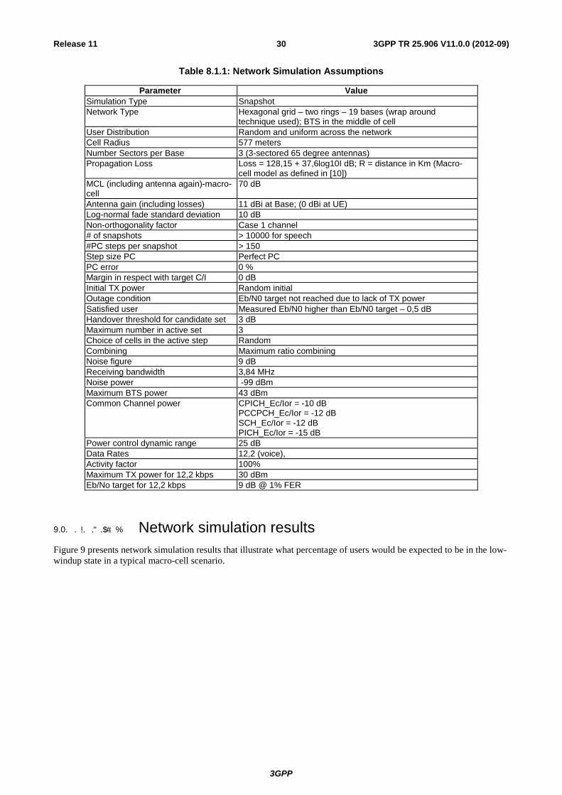
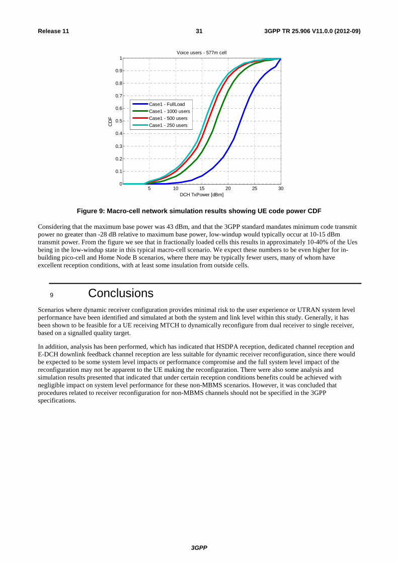
� � � �9.0. . . . .� �. Network simulation results Figure 9 presents network simulation results that illustrate what percentage of users would be expected to be in the low-windup state in a typical macro-cell scenario.

3GPP

3GPP TR 25.906 V11.0.0 (2012-09)31Release 11

5 10 15 20 25 300

0.1

0.2

0.3

0.4

0.5

0.6

0.7

0.8

0.9

1

DCH TxPower [dBm]

CD

F

Voice users - 577m cell

Case1 - FullLoadCase1 - 1000 usersCase1 - 500 usersCase1 - 250 users

Figure 9: Macro-cell network simulation results showing UE code power CDF

Considering that the maximum base power was 43 dBm, and that the 3GPP standard mandates minimum code transmit power no greater than -28 dB relative to maximum base power, low-windup would typically occur at 10-15 dBm transmit power. From the figure we see that in fractionally loaded cells this results in approximately 10-40% of the Ues being in the low-windup state in this typical macro-cell scenario. We expect these numbers to be even higher for in-building pico-cell and Home Node B scenarios, where there may be typically fewer users, many of whom have excellent reception conditions, with at least some insulation from outside cells.

9 Conclusions Scenarios where dynamic receiver configuration provides minimal risk to the user experience or UTRAN system level performance have been identified and simulated at both the system and link level within this study. Generally, it has been shown to be feasible for a UE receiving MTCH to dynamically reconfigure from dual receiver to single receiver, based on a signalled quality target.

In addition, analysis has been performed, which has indicated that HSDPA reception, dedicated channel reception and E-DCH downlink feedback channel reception are less suitable for dynamic receiver reconfiguration, since there would be expected to be some system level impacts or performance compromise and the full system level impact of the reconfiguration may not be apparent to the UE making the reconfiguration. There were also some analysis and simulation results presented that indicated that under certain reception conditions benefits could be achieved with negligible impact on system level performance for these non-MBMS scenarios. However, it was concluded that procedures related to receiver reconfiguration for non-MBMS channels should not be specified in the 3GPP specifications.

3GPP

3GPP TR 25.906 V11.0.0 (2012-09)32Release 11

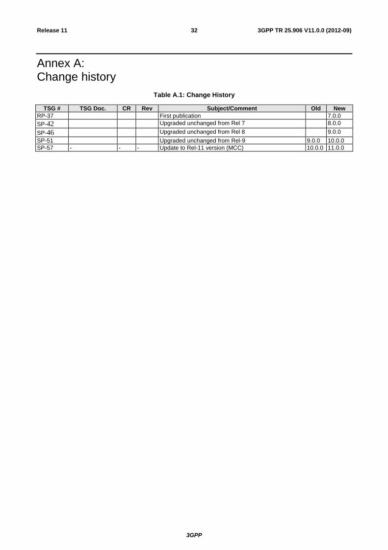
Annex A: Change history

Table A.1: Change History

TSG # TSG Doc. CR Rev Subject/Comment Old New RP-37 First publication 7.0.0 SP-42 Upgraded unchanged from Rel 7 8.0.0 SP-46 Upgraded unchanged from Rel 8 9.0.0 SP-51 Upgraded unchanged from Rel-9 9.0.0 10.0.0 SP-57 - - - Update to Rel-11 version (MCC) 10.0.0 11.0.0