I.1 Voter Behavior

Voters have to decide whether or not to turnout to

vote, who to vote for if they do turnout, and how

much information to acquire about the options they

face.

Economic theorists have addressed all these issues.

I.1.i Voter Turnout

Turnout refers to the fraction of eligible voters who

show up to vote.

In the U.S., there is considerable variation in turnout

both across and within types of elections.

Turnout is obviously key to understanding elections

because who shows up determines who wins.

In addition, from a strategic viewpoint parties are anx-

ious to “bring out their base” and this may impact the

type of candidates they run and/or the policy stances

they take.

There is a huge academic literature documenting and

trying to understand voter turnout - see Feddersen

(2004) for an excellent review.

Some Facts about Turnout

Voter turnout in the U.S. in the 2008 presidential elec-

tion was around 62%.

Voter turnout in the 2010 midterm elections was around

41%.

There is variation across states - for example, in the

2010 midterms turnout was 35% in New York and

55% in Maine.

Turnout in local elections, such as school board elec-

tions, can be extremely low (e.g., 10%) when they are

held separately from other elections.

Turnout tends to be higher for close races, where

closeness is measured by pre-election polls.

The likelihood of voting is positively correlated with

education, age, income, religiosity, and being married.

Some people are very regular voters, others sporadic,

and still others never vote.

Turnout can be influenced by campaigns.

Gerber and Green have done a series of field experi-

ments whereby they arrange with campaigns to pro-

vide different “treatments” to different groups of vot-

ers (see for example their paper in the 2000 American

Journal of Political Science).

Gerber and Green find, for example, that door-to-door

campaigning is very effective at getting people to turn

out.

Sending campaign material through the mail or calling

people on the phone is less effective.

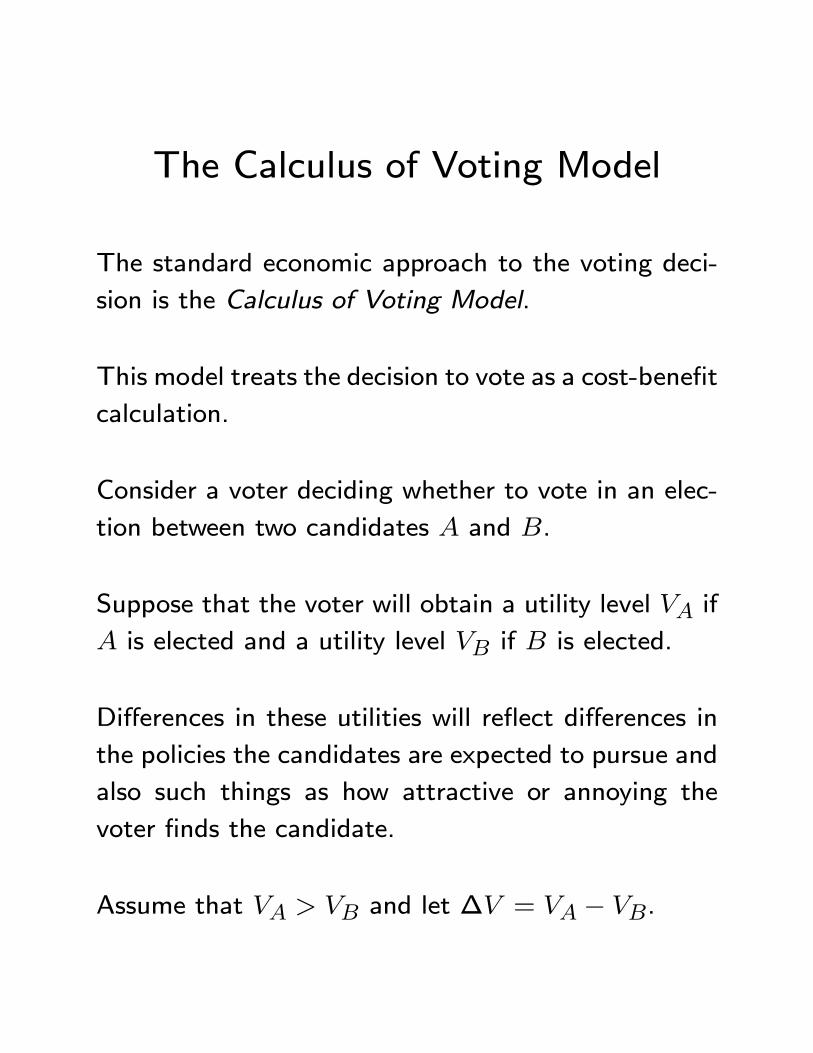
The Calculus of Voting Model

The standard economic approach to the voting deci-

sion is the Calculus of Voting Model.

This model treats the decision to vote as a cost-benefit

calculation.

Consider a voter deciding whether to vote in an elec-

tion between two candidates and .

Suppose that the voter will obtain a utility level if

is elected and a utility level if is elected.

Differences in these utilities will reflect differences in

the policies the candidates are expected to pursue and

also such things as how attractive or annoying the

voter finds the candidate.

Assume that and let ∆ = − .

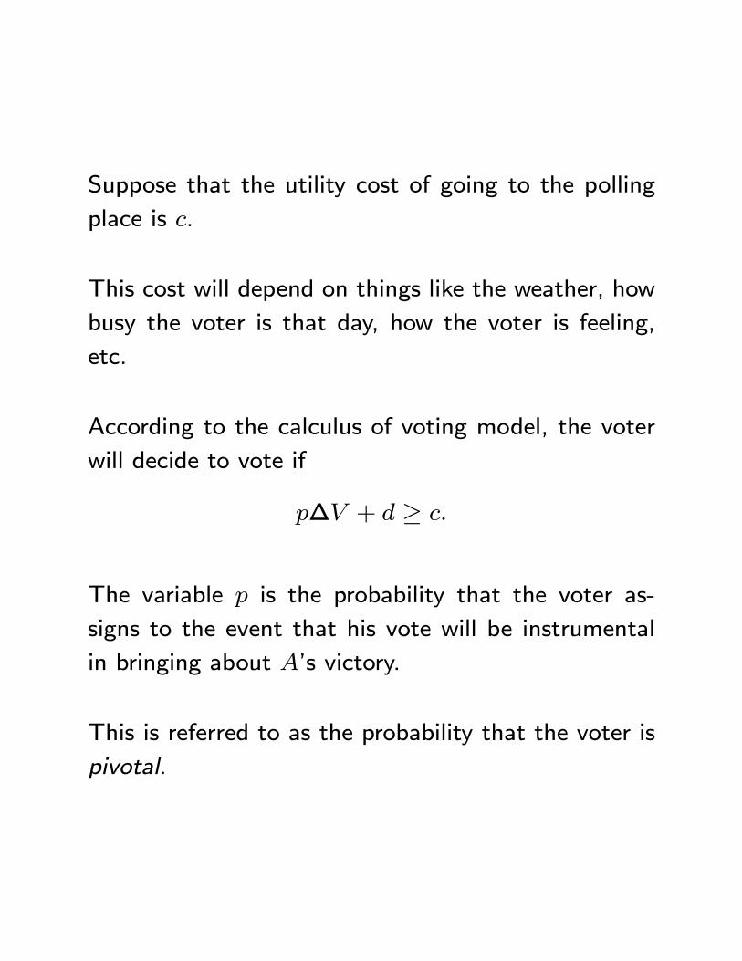
Suppose that the utility cost of going to the polling

place is .

This cost will depend on things like the weather, how

busy the voter is that day, how the voter is feeling,

etc.

According to the calculus of voting model, the voter

will decide to vote if

∆ + ≥

The variable is the probability that the voter as-

signs to the event that his vote will be instrumental

in bringing about ’s victory.

This is referred to as the probability that the voter is

pivotal.

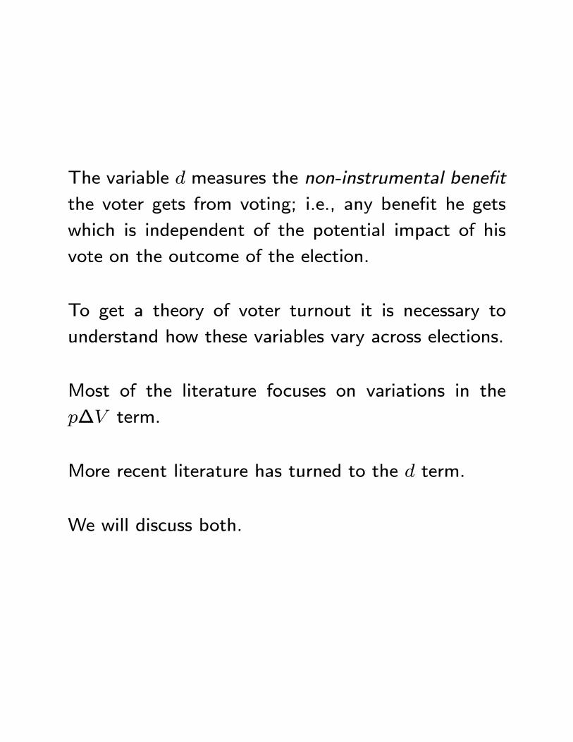
The variable measures the non-instrumental benefit

the voter gets from voting; i.e., any benefit he gets

which is independent of the potential impact of his

vote on the outcome of the election.

To get a theory of voter turnout it is necessary to

understand how these variables vary across elections.

Most of the literature focuses on variations in the

∆ term.

More recent literature has turned to the term.

We will discuss both.

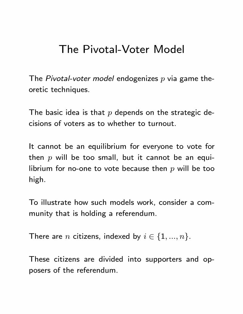
The Pivotal-Voter Model

The Pivotal-voter model endogenizes via game the-

oretic techniques.

The basic idea is that depends on the strategic de-

cisions of voters as to whether to turnout.

It cannot be an equilibrium for everyone to vote for

then will be too small, but it cannot be an equi-

librium for no-one to vote because then will be too

high.

To illustrate how such models work, consider a com-

munity that is holding a referendum.

There are citizens, indexed by ∈ {1 }.

These citizens are divided into supporters and op-

posers of the referendum.

Supporters are each willing to pay for the proposed

change, while opposers are each willing to pay to

avoid it.

Each citizen knows whether he is a supporter or an

opposer, but does not know the number of citizens in

each category.

All citizens know that the probability that a randomly

selected individual is a supporter is .

Citizens must decide whether to not to vote in the

referendum.

If they do vote, supporters vote in favor and opposers

vote against.

If the number of votes in favor of the referendum is

at least as big as the number against, the proposed

change is approved.

Each citizen’s cost of voting on the day of the refer-

endum is ex ante uncertain.

This reflects the fact that the voting cost will depend

on idiosyncratic stuff such as how the citizen as feel-

ing, whether his car is working, etc.

We will model this by assuming that citizen ’s cost

of voting is the realization of a random variable

distributed on [0 max] with CDF ().

Each citizen observes his own voting cost.

However, he only knows that the costs of his fellows

are the independent realizations of −1 random vari-

ables distributed on [0 max] according to ().

The pivotal-voter model assumes that the only benefit

of voting is the instrumental benefit of changing the

outcome.

Since the probability of being pivotal depends upon

who else is voting, voting is a strategic decision.

Accordingly, the situtation is modelled as a game of

incomplete information.

The incomplete information concerns the preferences

and voting costs of the other voters.

A strategy for a citizen is a function which for each

possible realization of his voting cost specifies whether

he will vote or abstain.

The equilibrium concept is Bayesian Nash equilibrium.

Roughly speaking, every citizen must be happy with

his strategy given he knows (i) what strategies others

are playing and (ii) the statistical information and

().

Equilibrium

We look for a symmetric equilibrium in which all sup-

porters use the same strategy and all opposers use the

same strategy.

With no loss of generality, we can assume that sup-

porters and opposers use “cut-off” strategies that spec-

ify that they vote if and only if their cost of voting is

below some critical level.

Accordingly, a symmetric equilibrium is characterized

by a pair of numbers ∗ and ∗ representing the cut-off cost levels of the two groups.

To characterize the equilibrium cut-off levels, consider

the situation of some individual .

Suppose that the remaining −1 individuals are play-ing according to the equilibrium strategies; i.e., if they

are supporters (opposers) they vote if their voting cost

is less than ∗ (∗).

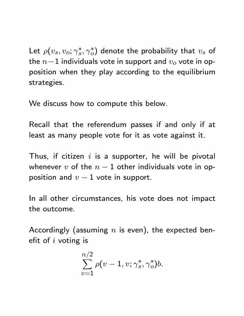
Let ( ; ∗

∗) denote the probability that of

the −1 individuals vote in support and vote in op-position when they play according to the equilibrium

strategies.

We discuss how to compute this below.

Recall that the referendum passes if and only if at

least as many people vote for it as vote against it.

Thus, if citizen is a supporter, he will be pivotal

whenever of the − 1 other individuals vote in op-position and − 1 vote in support.

In all other circumstances, his vote does not impact

the outcome.

Accordingly (assuming is even), the expected ben-

efit of voting is

2X=1

( − 1 ; ∗ ∗)

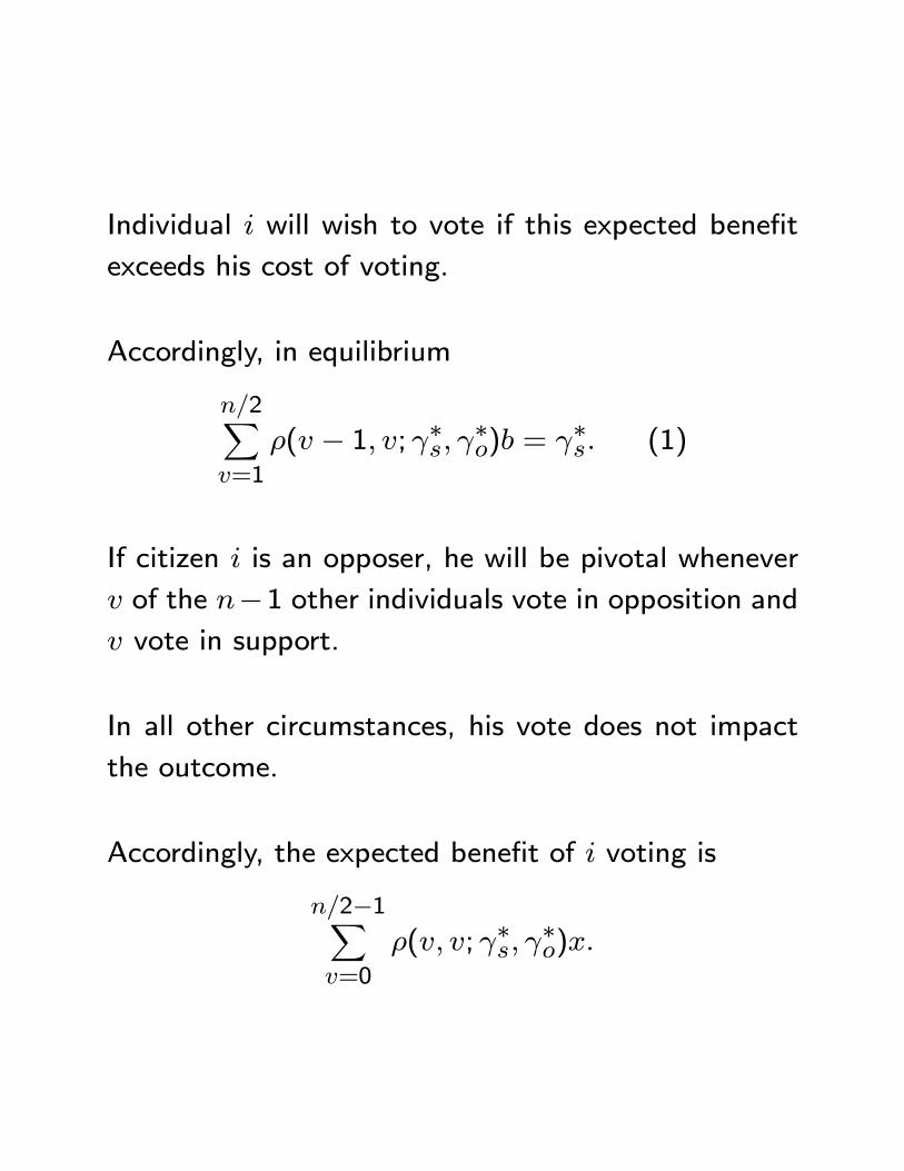
Individual will wish to vote if this expected benefit

exceeds his cost of voting.

Accordingly, in equilibrium

2X=1

( − 1 ; ∗ ∗) = ∗ (1)

If citizen is an opposer, he will be pivotal whenever

of the −1 other individuals vote in opposition and vote in support.

In all other circumstances, his vote does not impact

the outcome.

Accordingly, the expected benefit of voting is

2−1X=0

( ; ∗ ∗)

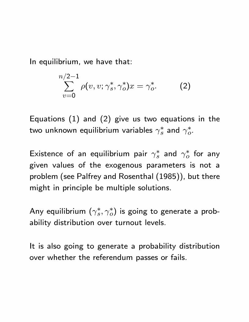
In equilibrium, we have that:

2−1X=0

( ; ∗ ∗) = ∗ (2)

Equations (1) and (2) give us two equations in the

two unknown equilibrium variables ∗ and ∗.

Existence of an equilibrium pair ∗ and ∗ for anygiven values of the exogenous parameters is not a

problem (see Palfrey and Rosenthal (1985)), but there

might in principle be multiple solutions.

Any equilibrium (∗ ∗) is going to generate a prob-ability distribution over turnout levels.

It is also going to generate a probability distribution

over whether the referendum passes or fails.

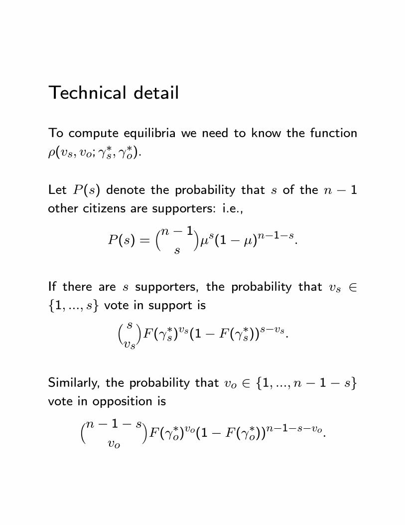
Technical detail

To compute equilibria we need to know the function

( ; ∗

∗).

Let () denote the probability that of the − 1other citizens are supporters: i.e.,

() =³− 1

´(1− )−1−

If there are supporters, the probability that ∈{1 } vote in support is³

´ (∗)(1− (∗))−

Similarly, the probability that ∈ {1 − 1 − }vote in opposition is³− 1−

´ (∗)(1− (∗))−1−−

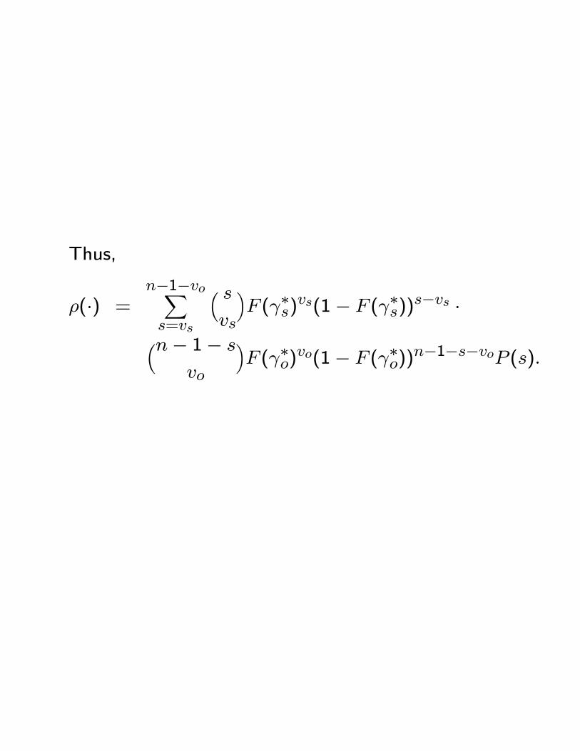
Thus,

(·) =−1−X=

³

´ (∗)(1− (∗))− ·³− 1−

´ (∗)(1− (∗))−1−− ()

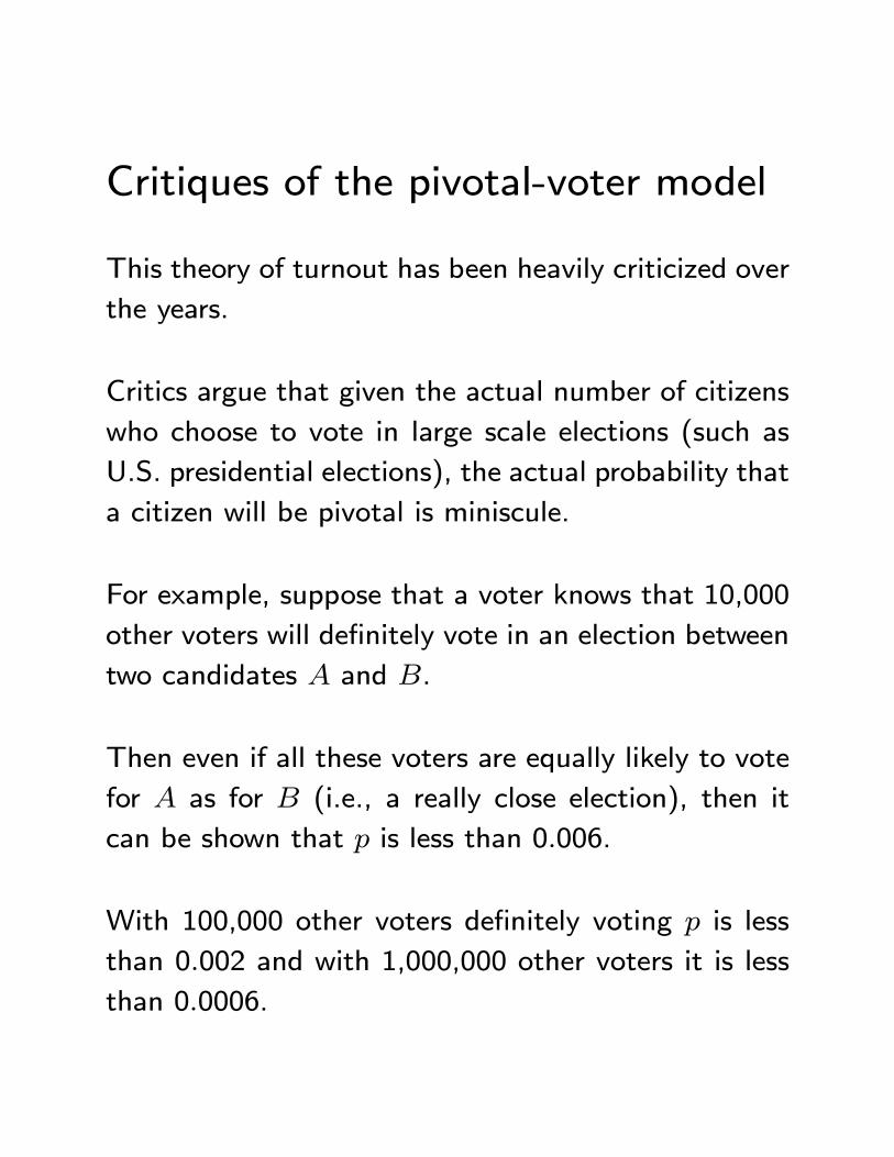
Critiques of the pivotal-voter model

This theory of turnout has been heavily criticized over

the years.

Critics argue that given the actual number of citizens

who choose to vote in large scale elections (such as

U.S. presidential elections), the actual probability that

a citizen will be pivotal is miniscule.

For example, suppose that a voter knows that 10,000

other voters will definitely vote in an election between

two candidates and .

Then even if all these voters are equally likely to vote

for as for (i.e., a really close election), then it

can be shown that is less than 0006.

With 100,000 other voters definitely voting is less

than 0002 and with 1,000,000 other voters it is less

than 00006.

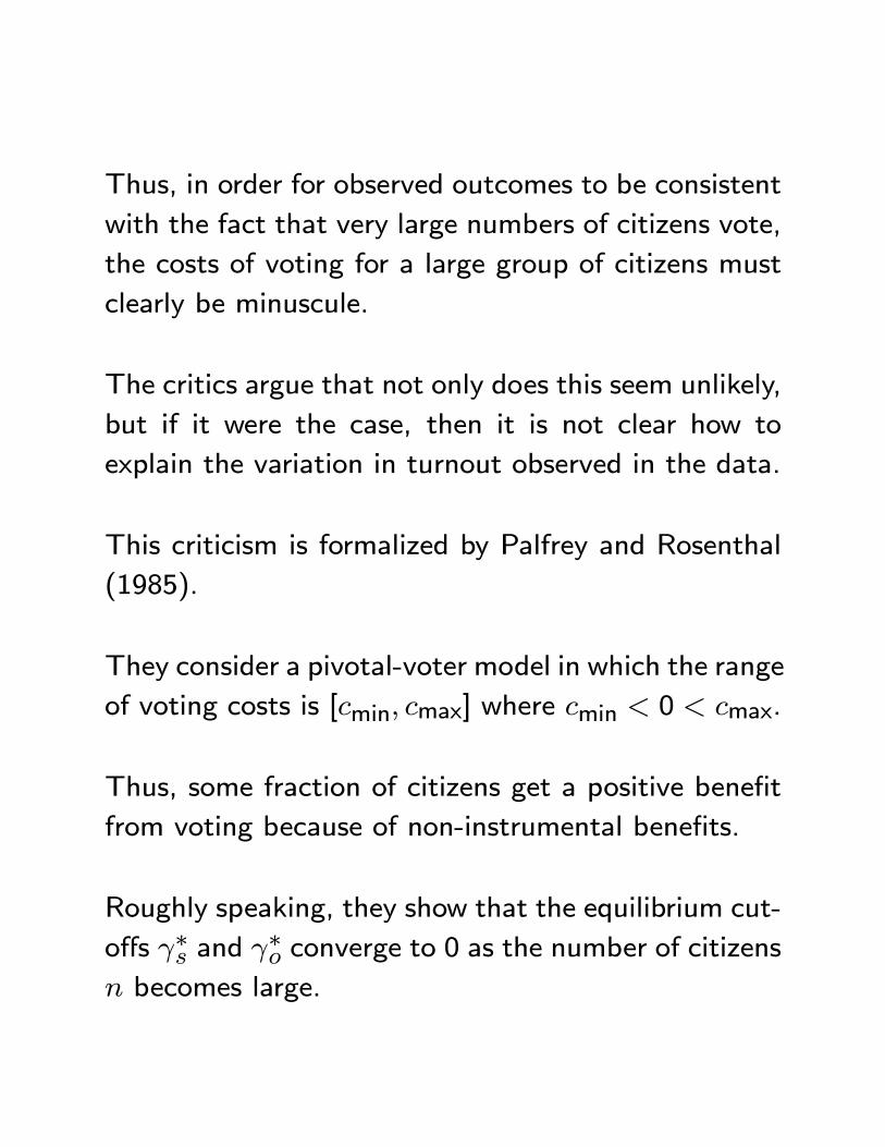
Thus, in order for observed outcomes to be consistent

with the fact that very large numbers of citizens vote,

the costs of voting for a large group of citizens must

clearly be minuscule.

The critics argue that not only does this seem unlikely,

but if it were the case, then it is not clear how to

explain the variation in turnout observed in the data.

This criticism is formalized by Palfrey and Rosenthal

(1985).

They consider a pivotal-voter model in which the range

of voting costs is [min max] where min 0 max.

Thus, some fraction of citizens get a positive benefit

from voting because of non-instrumental benefits.

Roughly speaking, they show that the equilibrium cut-

offs ∗ and ∗ converge to 0 as the number of citizens becomes large.

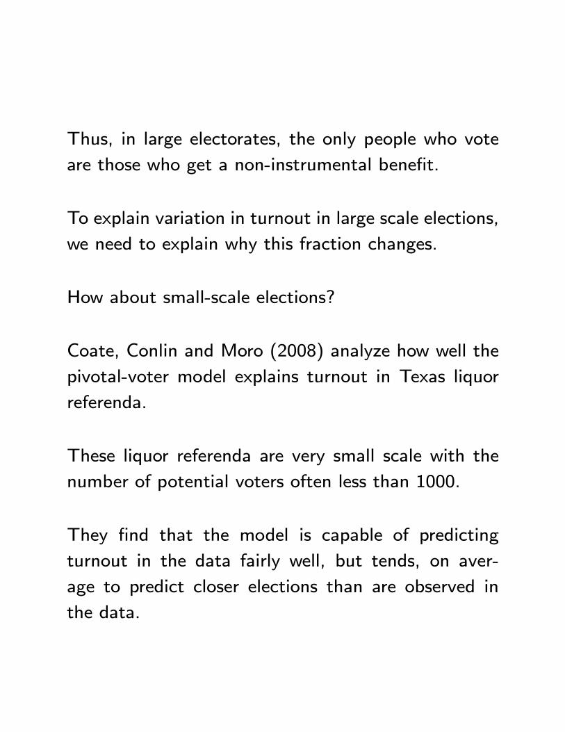
Thus, in large electorates, the only people who vote

are those who get a non-instrumental benefit.

To explain variation in turnout in large scale elections,

we need to explain why this fraction changes.

How about small-scale elections?

Coate, Conlin and Moro (2008) analyze how well the

pivotal-voter model explains turnout in Texas liquor

referenda.

These liquor referenda are very small scale with the

number of potential voters often less than 1000.

They find that the model is capable of predicting

turnout in the data fairly well, but tends, on aver-

age to predict closer elections than are observed in

the data.

The pivotal-voter logic implies that elections must be

expected to be close even if there is a significant dif-

ference between the sizes of the groups supporting the

candidates or the intensity of their preferences.

With a very small number of eligible voters, elections

that are expected to be close ex ante may end up not

close ex post because of sampling error.

For example, an unexpectedly large number of eligi-

ble voters may favor one side of the issue or, alter-

natively, a disproportionate number of eligible voters

on one side of the issue may receive low voting cost

realizations.

As the number of eligible voters increases, this sam-

pling error very quickly disappears and elections that

are expected to be close ex ante will be close ex post.

However, in the data, winning margins can be signifi-

cant even in the larger elections.

This suggests that the model does not work for either

large or small-scale elections.

Defense of the pivotal-voter model

Despite these criticisms, the pivotal-voter theory re-

mains a core model in formal political science.

It is in many respects the simplest and most natural

way of thinking about turnout.

Moreover, the basic idea that turnout should be higher

in elections that are expected to be close is borne out

in the data (see, for example, Shachar and Nalebuff

(1999)).

In addition, Levine and Palfrey (2007) find in their

experimental study of voter turnout that three key

comparative static predictions of the theory are bourne

out in the data.

These are: (i) the size effect whereby turnout goes

down in large elections,

(ii) the competition effect whereby turnout is higher

in elections that are expected to be close, and

(iii) the underdog effect whereby turnout rates are

higher among voters supporting the less popular al-

ternative.

Duffy and Tavits (2008) run a voting experiment that

allows them to elicit peoples’ beliefs about the likeli-

hood that their votes will be pivotal.

They find support for the idea that people who believe

that there is higher chance their vote will be pivotal

are more likely to vote.

They also find that people substantially overestimate

the chance that their votes will be pivotal.

This seems consistent with the fact that popular rhetoric

encouraging citizens to participate politically typically

stresses the idea that every individual’s vote counts.

Still, surveys find that while people do overestimate

their chances of being pivotal, they are not way off on

this.

Expressive Voting

Dissatisfaction with the pivotal-voter model has led

researchers to turn to theorize about the determinants

of the -term (i.e., the non-instrumental benefit of

voting).

One way to think about is that it is the benefit the

voter gets from expressing his preferences.

According to the expressive view, voting is like cheer-

ing at a football game: you do not cheer because you

think it is going to impact the outcome, you do it

because the game is exciting and cheering is fun.

Under this view, it is natural to assume that will de-

pend on how strongly the voter feels about the can-

didates and also how close the election is going to

be.

After all, people cheer harder when they care a lot

about their team winning and also when the game is

close.

Thus, assuming that in a closer election will be

higher, we might write = (∆ ) where (·) isa function with the property that ∆ 0 and

0.

Such a model would then predict that turnout would

be higher in elections which are close and in which

people feel strongly about the candidates.

It would also be natural to assume that being con-

tacted by a candidate or having more media attention

devoted to a race would raise peoples’ expressive ben-

efits.

Thus this view is capable of generating predictions

consistent with the facts discussed above.

Voting as Civic Duty

Another way to think about the term is that it rep-

resents the payoff of doing your civic “duty”.

The idea is that we are taught in civics classes that

we should vote and thus we get a “warm-glow” feeling

when we do vote (or perhaps avoid feeling guilty!).

Survey evidence reveals that a significant fraction of

voters (50%) feel that voting is a moral obligation and

would feel guilty if they did not vote.

However, the fact that people turn out in much lower

rates in local elections suggests that either the payoff

from doing one’s duty depends on the type of election

under consideration, or perhaps that it is not one’s

duty to vote in school board elections or elections for

town sheriff.

All this suggests that to operationalize this civic duty

view we need (i) a theory of what one’s duty as a citi-

zen is, and (ii) a theory which tells us what determines

the warm-glow from doing one’s civic duty.

A Rule Utilitarian View of Duty

One interesting perspective on (i) (i.e., what doing

one’s duty is) comes from the idea of behaving as a

rule utilitarian.

A rule utilitarian follows the rule of behavior that if

everyone else also followed would maximize aggregate

societal utility.

For example, consider the decision as to whether to

throw your MacDonald’s burger wrapper out of your

car.

A standard economic agent would throw it out of his

car, reasoning that his one wrapper would do little

damage to the environment, but would save him the

trouble of putting it in the trash when he got home.

A rule utilitarian would think through to the environ-

mental damage that would happen if everyone threw

their wrappers out of their cars and would thus refrain

from so doing.

The interesting thing is that the rule utilitarian would

not necessarily always vote.

A simple example will illustrate the point.

Consider a society of 2 citizens, Mr 1 and Mr 2.

Suppose that the society is holding a referendum to

approve some policy reform.

The reform will be approved if at least one citizen

votes in favor.

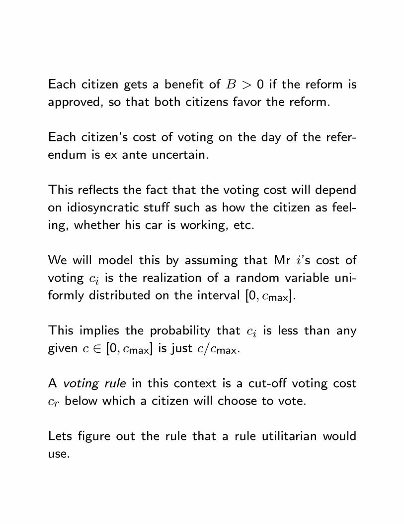
Each citizen gets a benefit of 0 if the reform is

approved, so that both citizens favor the reform.

Each citizen’s cost of voting on the day of the refer-

endum is ex ante uncertain.

This reflects the fact that the voting cost will depend

on idiosyncratic stuff such as how the citizen as feel-

ing, whether his car is working, etc.

We will model this by assuming that Mr ’s cost of

voting is the realization of a random variable uni-

formly distributed on the interval [0 max].

This implies the probability that is less than any

given ∈ [0 max] is just max.

A voting rule in this context is a cut-off voting cost

below which a citizen will choose to vote.

Lets figure out the rule that a rule utilitarian would

use.

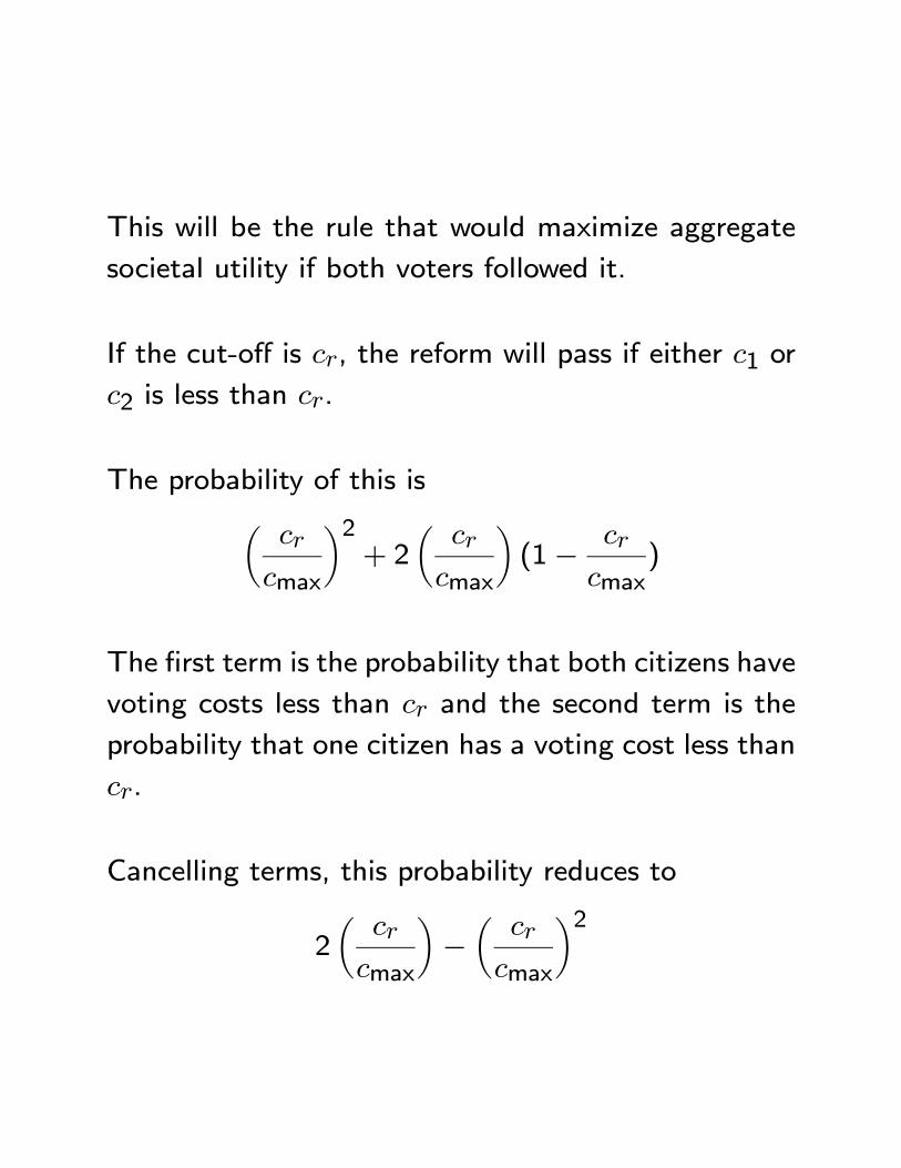
This will be the rule that would maximize aggregate

societal utility if both voters followed it.

If the cut-off is , the reform will pass if either 1 or

2 is less than .

The probability of this isµ

max

¶2+ 2

µ

max

¶(1−

max)

The first term is the probability that both citizens have

voting costs less than and the second term is the

probability that one citizen has a voting cost less than

.

Cancelling terms, this probability reduces to

2

µ

max

¶−µ

max

¶2

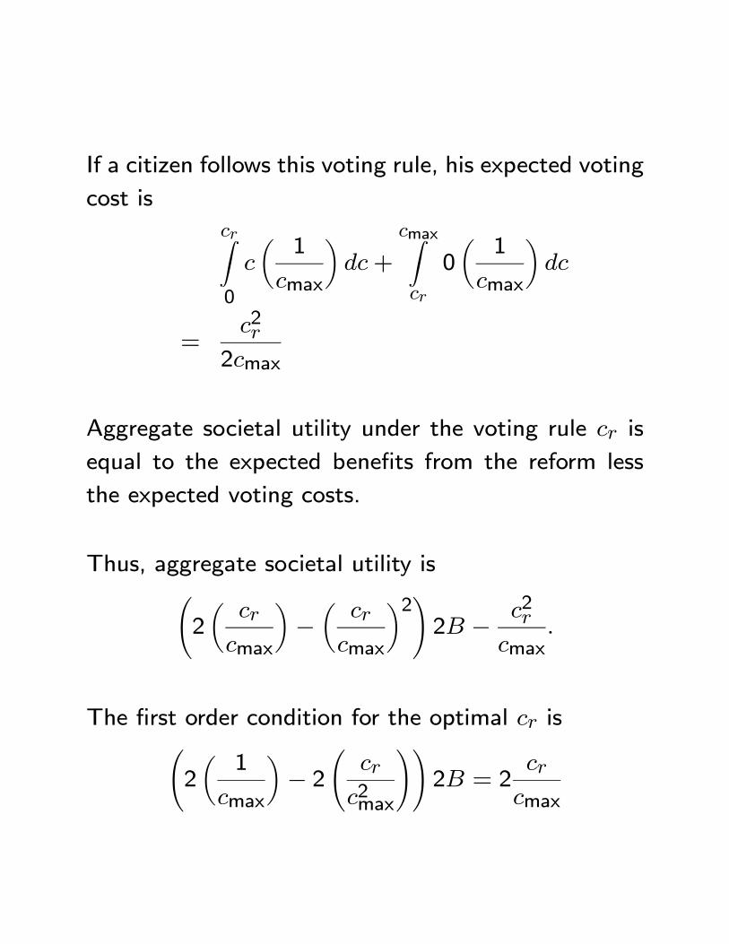
If a citizen follows this voting rule, his expected voting

cost is

Z0

µ1

max

¶+

maxZ

0

µ1

max

¶

=2

2max

Aggregate societal utility under the voting rule is

equal to the expected benefits from the reform less

the expected voting costs.

Thus, aggregate societal utility isÃ2

µ

max

¶−µ

max

¶2!2 − 2

max

The first order condition for the optimal isÃ2

µ1

max

¶− 2

Ã

2max

!!2 = 2

max

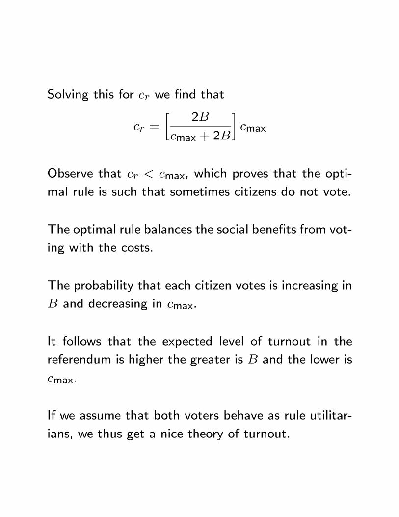
Solving this for we find that

=

∙2

max + 2

¸max

Observe that max, which proves that the opti-

mal rule is such that sometimes citizens do not vote.

The optimal rule balances the social benefits from vot-

ing with the costs.

The probability that each citizen votes is increasing in

and decreasing in max.

It follows that the expected level of turnout in the

referendum is higher the greater is and the lower is

max.

If we assume that both voters behave as rule utilitar-

ians, we thus get a nice theory of turnout.

This example is special in the sense that all citizens

benefit from the policy reform.

In most elections, there is disagreement and the role

of the election is to resolve this disagreement.

The rule utilitarian perspective can be generalized to

deal with this case.

Feddersen and Sandroni (2006) develop a theory of

turnout in two candidate elections based on the idea

that rule utilitarians differ in the candidate who they

believe maximizes aggregate utility.

They assume that there are two groups of rule utili-

tarians with differing views.

One group believes that one candidate is best for the

country, the other group believes the other candidate

is best.

Individuals in each group choose their voting rule tak-

ing as given the behavior of the other group.

A related model is investigated by Coate and Conlin

(2004) who assume that individuals are motivated to

vote by the ethical desire to “do their part” to help

their side win.

Thus, individuals follow the voting rule that, if fol-

lowed by everyone else on their side of the issue, would

maximize their side’s aggregate utility.

Individuals therefore act as group rule-utilitarians, with

their groups being those who share their position.

Coate and Conlin (2004) analyze how well this group

rule-utilitarian model explains turnout in Texas liquor

referenda.

They find that the comparative static predictions of

the model are consistent with the data.

They also structurally estimate the model and show

that it out-performs a very simple expressive voting

model in which a voter’s benefit from expressing a

preference just depends on how strongly he feels about

the issue.

Thus, thinking about how a rule utilitarian would vote

seems to provide a promising theory of what one’s

duty as a citizen is when it comes to voting.

This still leaves us with the second part of the problem

(i.e., (ii)) which is to find a theory which tells us what

determines the warm-glow from doing one’s civic duty.

Gerber, Green and Larimer (2008) have a very in-

teresting empirical finding that mailings promising to

publicize individuals’ turnout to their neighbors led to

substantially higher turnout.

This perhaps suggests that the warm-glow from do-

ing one’s duty partly comes from knowing that others

know we did our duty.

I.1.ii Voting in Multicandidate Elec-tions

In elections with three or more candidates, there is an

important distinction between sincere and strategic

voting.

To illustrate the distinction, consider an election in

which there are three candidates and .

Suppose there are voters labeled voter 1, voter 2,

etc.

Let voter ’s utility if candidate is elected be denoted

.

Assume that all voters vote and let ∈ {}denote voter ’s decision as to who to vote for; i.e., if

= , voter votes for candidate .

Let (1 ) denote the voting decisions of all the

voters.

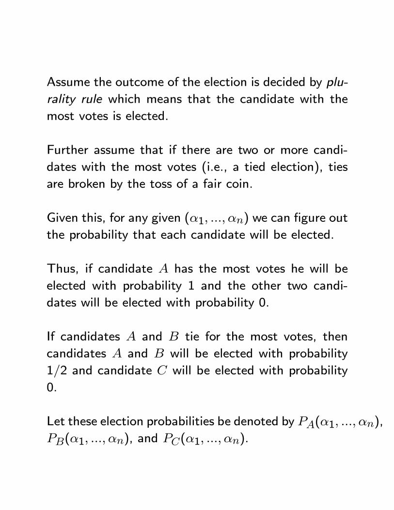
Assume the outcome of the election is decided by plu-

rality rule which means that the candidate with the

most votes is elected.

Further assume that if there are two or more candi-

dates with the most votes (i.e., a tied election), ties

are broken by the toss of a fair coin.

Given this, for any given (1 ) we can figure out

the probability that each candidate will be elected.

Thus, if candidate has the most votes he will be

elected with probability 1 and the other two candi-

dates will be elected with probability 0.

If candidates and tie for the most votes, then

candidates and will be elected with probability

12 and candidate will be elected with probability

0.

Let these election probabilities be denoted by (1 ),

(1 ), and (1 ).

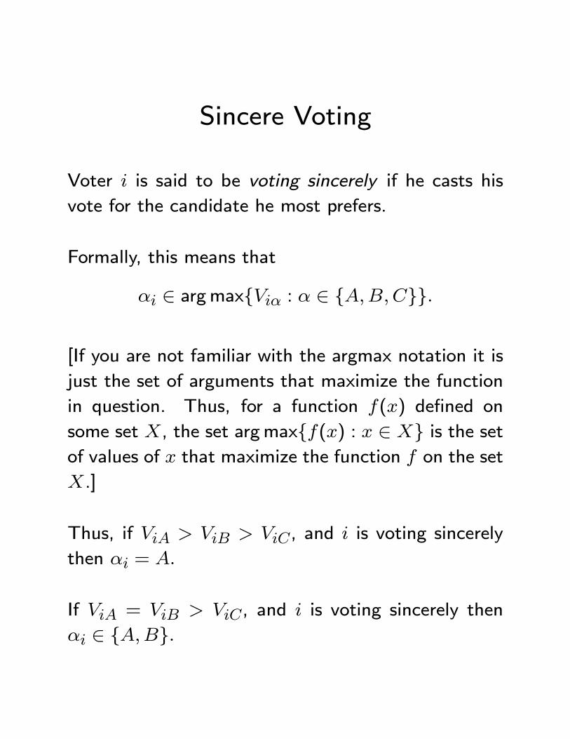
Sincere Voting

Voter is said to be voting sincerely if he casts his

vote for the candidate he most prefers.

Formally, this means that

∈ argmax{ : ∈ {}}

[If you are not familiar with the argmax notation it is

just the set of arguments that maximize the function

in question. Thus, for a function () defined on

some set , the set argmax{() : ∈ } is the setof values of that maximize the function on the set

.]

Thus, if , and is voting sincerely

then =

If = , and is voting sincerely then

∈ {}

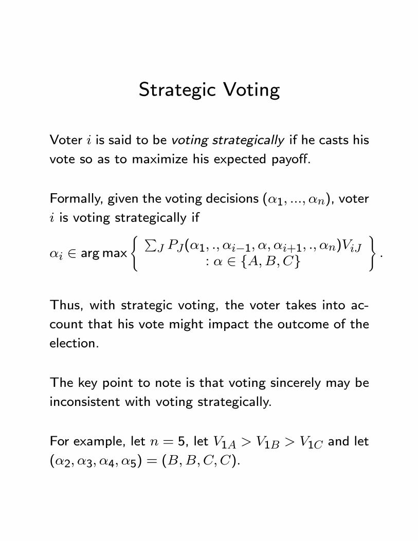
Strategic Voting

Voter is said to be voting strategically if he casts his

vote so as to maximize his expected payoff.

Formally, given the voting decisions (1 ), voter

is voting strategically if

∈ argmax( P

(1 −1 +1 ): ∈ {}

)

Thus, with strategic voting, the voter takes into ac-

count that his vote might impact the outcome of the

election.

The key point to note is that voting sincerely may be

inconsistent with voting strategically.

For example, let = 5, let 1 1 1 and let

(2 3 4 5) = ().

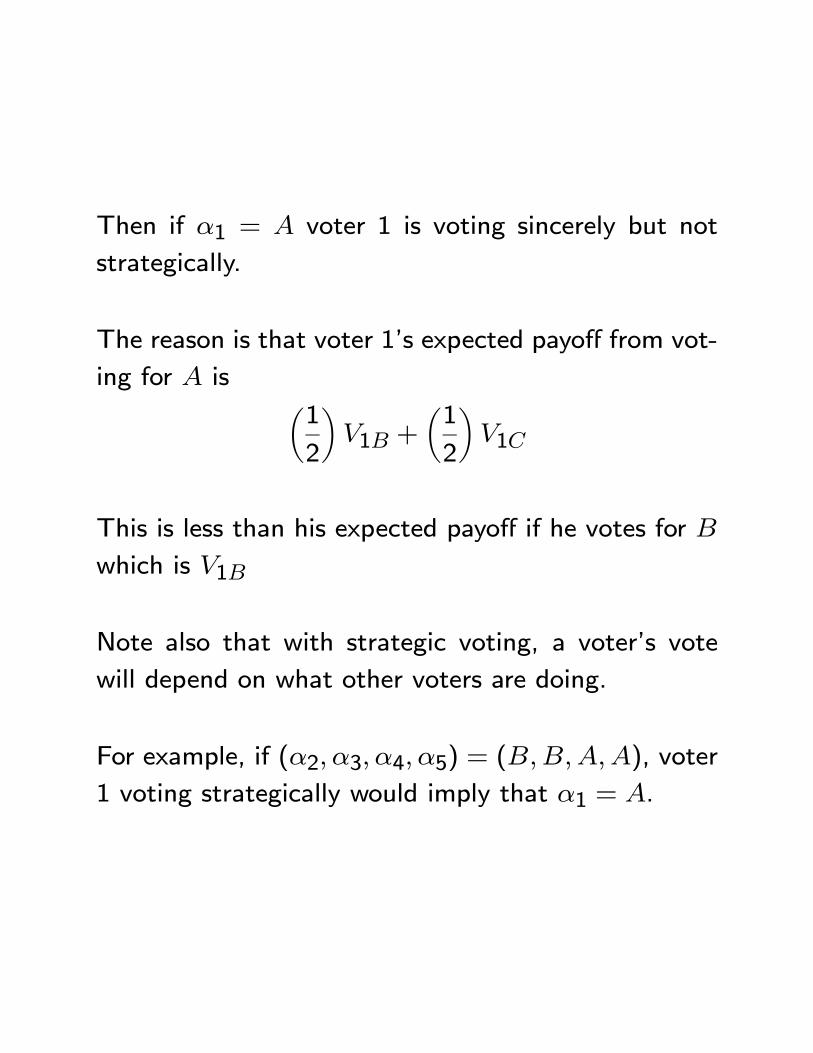
Then if 1 = voter 1 is voting sincerely but not

strategically.

The reason is that voter 1’s expected payoff from vot-

ing for is µ1

2

¶1 +

µ1

2

¶1

This is less than his expected payoff if he votes for

which is 1

Note also that with strategic voting, a voter’s vote

will depend on what other voters are doing.

For example, if (2 3 4 5) = (), voter

1 voting strategically would imply that 1 = .

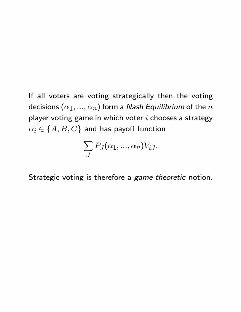
If all voters are voting strategically then the voting

decisions (1 ) form a Nash Equilibrium of the

player voting game in which voter chooses a strategy

∈ {} and has payoff functionX

(1 )

Strategic voting is therefore a game theoretic notion.

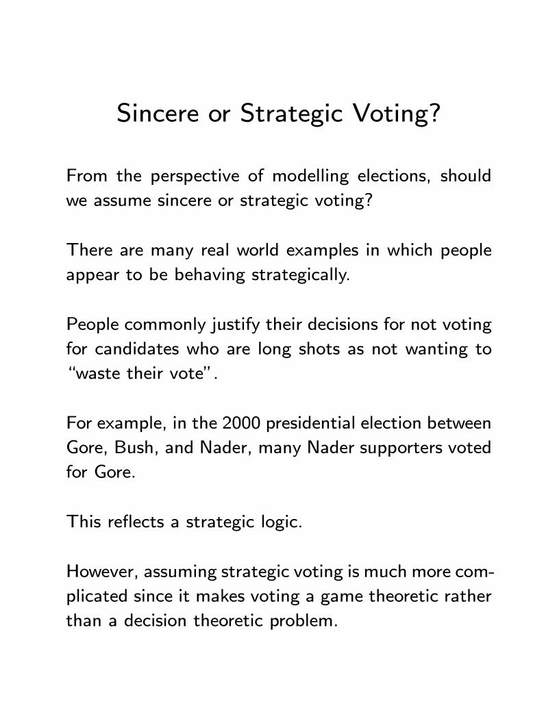
Sincere or Strategic Voting?

From the perspective of modelling elections, should

we assume sincere or strategic voting?

There are many real world examples in which people

appear to be behaving strategically.

People commonly justify their decisions for not voting

for candidates who are long shots as not wanting to

“waste their vote”.

For example, in the 2000 presidential election between

Gore, Bush, and Nader, many Nader supporters voted

for Gore.

This reflects a strategic logic.

However, assuming strategic voting is much more com-

plicated since it makes voting a game theoretic rather

than a decision theoretic problem.

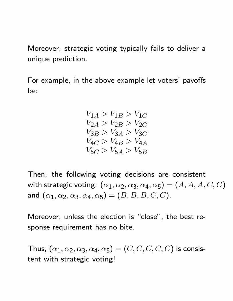
Moreover, strategic voting typically fails to deliver a

unique prediction.

For example, in the above example let voters’ payoffs

be:

1 1 12 2 23 3 34 4 45 5 5

Then, the following voting decisions are consistent

with strategic voting: (1 2 3 4 5) = ()

and (1 2 3 4 5) = ().

Moreover, unless the election is “close”, the best re-

sponse requirement has no bite.

Thus, (1 2 3 4 5) = () is consis-

tent with strategic voting!

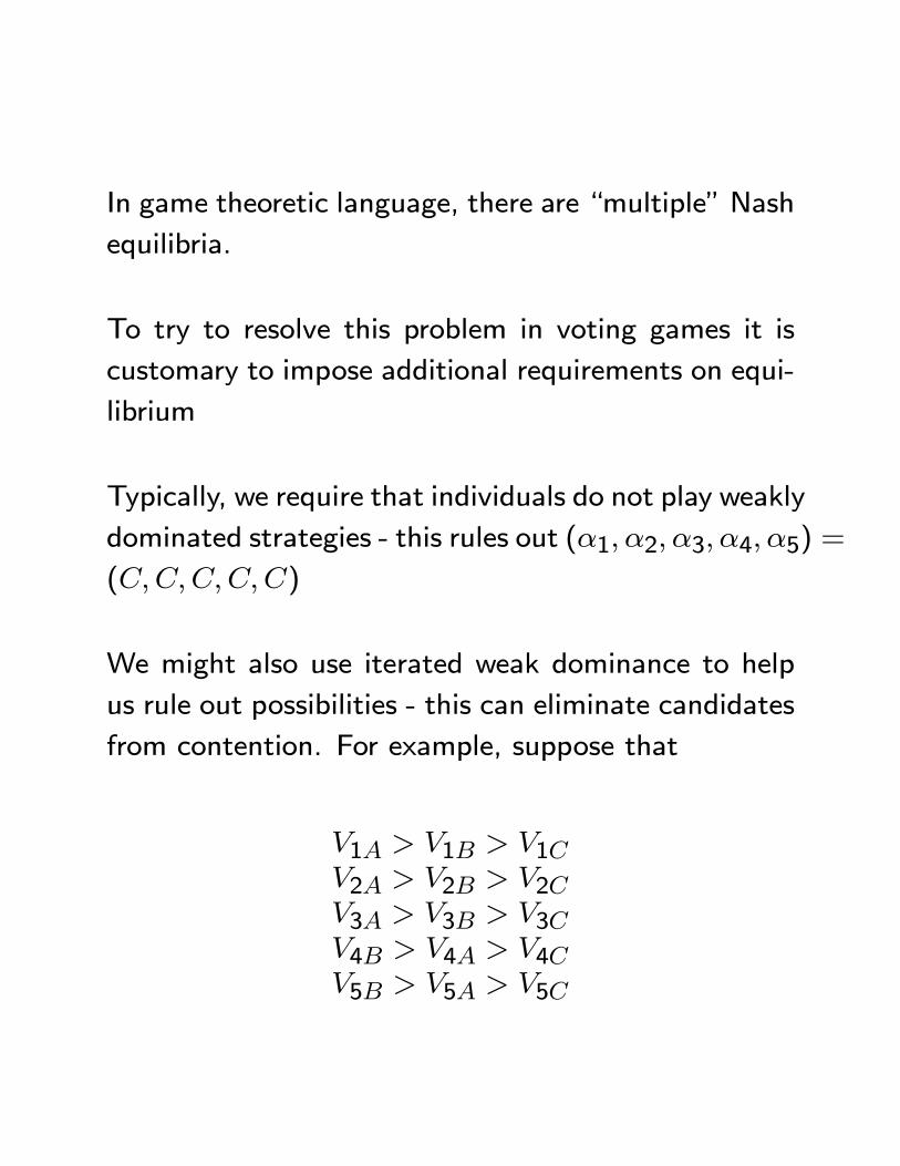
In game theoretic language, there are “multiple” Nash

equilibria.

To try to resolve this problem in voting games it is

customary to impose additional requirements on equi-

librium

Typically, we require that individuals do not play weakly

dominated strategies - this rules out (1 2 3 4 5) =

()

We might also use iterated weak dominance to help

us rule out possibilities - this can eliminate candidates

from contention. For example, suppose that

1 1 12 2 23 3 34 4 45 5 5

Then the first round of eliminating weakly dominated

strategies eliminates from contention.

The second round implies that (1 2 3 4 5) =

()

Another approach is to introduce population uncer-

tainty to give the best response requirement more bite.

This helps matters somewhat but does not resolve

the basic indeterminancy exhibited in the above exam-

ple where voters can coalesce around one or another

candidate (i.e., (1 2 3 4 5) = ()

and (1 2 3 4 5) = ()).

Such indeterminacy seems somewhat realistic.

For example, in the 2008 Democratic primary, would

anti-Hilary Clinton Democrats vote for Obama or Ed-

wards?

This was by no means clear early in the campaign.

In reality, such issues seems to be determined dynam-

ically with the help of polls and some coordination

among like-minded citizens.

Also candidates may withdraw to shift their supporters

to a like-minded candidate.

Myatt (2007) uses techniques from the theory of global

games to resolve the indeterminacy.

Sophisticated vs Simple SincereVoting

Even in a two-candidate election, there some ambigu-

ity in defining what is meant by sincere voting.

This is the case when the elected candidate will de-

termine policy collectively with others - for example,

when electing a legislator to a legislature.

To illustrate, consider electing a U.S. senator.

Consider a centrist voter choosing between a moder-

ate Republican and a left wing Democrat.

Suppose that policy-making in the Senate is deter-

mined by the party that holds the majority of seats

and reflects a compromise between the Senators in

the majority party.

Suppose that the Republicans currently hold the ma-

jority in the Senate and that most of the Republican

senators are right wing Republicans.

Further suppose that most of the Democrat senators

are moderate Democrats.

Simple sincere voting would involve the voter voting

for the candidate who is closest to his own position;

i.e., the Republican.

Sophisticated sincere voting would involve the voter

anticipating how the candidate would impact policy-

making in the Senate and voting for the candidate

whose election would yield the preferred policy out-

come.

This could involve voting for the Democrat.

The logic is as follows: electing the Democrat could

help switch the Senate from Republican to Democrat

control and, since most Democrat senators are moder-

ates, this would result in moderate Democrat policies

as opposed to right wing Republican policies.

This logic appeared to be behind the loss of moderate

Republican Senator Lincoln Chaffee (Rhode Island) in

the 2006 mid-term elections.

A related phenomenon is “ticket splitting”, which arises

when a voter votes for, say, the Democratic presiden-

tial candidate and the Republican congressional can-

didate.

This is quite a common phenomenon in fact and the

literature discusses at length what might be going on.

It could be just simple sincere voting and reflect the

fact that candidates in the same party have different

ideologies.

It could alternatively be sophisticated sincere voting

in which voters are trying to achieve the right balance

between the ideology of Congress and the president.

For example, a moderate voter may prefer a divided

government (e.g., Democrat congress and Republican

president) to a unified government (i.e., all Republican

or all Democrat).

Finally, it could actually be real strategic voting where

voters are taking into account the probability of im-

pacting the outcome.

See Morton’s book (pp523-529), Burden and Kim-

ball (1998), Degan and Merlo (2009), and Lacy and

Paolini (1998) for more on this topic.

I.1.iii Voter Information

In addition to deciding whether or not to vote and to

deciding for whom to vote, voters also have to decide

how much information to acquire.

How much do voters actually know about the candi-

dates and/or issues they are voting on?

In general, surveys reveal that voters do not know

much at all about politics.

Around 50% of Americans do not know that each

state has two senators and 40% cannot name either

of their senators.

Over 50% cannot name their congressman and only

about 50% know which party controls the House.

The fact that voters do not know much is perfectly

consistent with an economic approach.

If acquiring information about politics is costly for vot-

ers, then we should expect them to remain rationally

ignorant.

The benefit of acquiring political information is small

because there is almost no chance of a voter’s decision

changing the outcome.

Thus, we would only expect voters to have such in-

formation as can be costlessly acquired (say through

tv commercials) or which they enjoy acquiring (like

information about scandals)

Significance of Rational Ignorance

Despite rational ignorance, many political scientists

argue that voters are able to choose which candidate

or policy option is best for them.

There are three distinct arguments.

First, there are plenty of easily acquired signals that

voters can use to make the correct choices.

Such signals include party affiliations, newspaper en-

dorsements, endorsements from interest groups, ad-

vice from informed friends and relatives, etc.

Second, those who are uninformed are less likely to

participate.

There is a great deal of evidence that the less infor-

mation people have about the options on the ballot

the less likely they are to show up to vote.

Indeed, it is common for people not to vote when they

lack information even when voting is costless.

This is evidenced by the phenomenon of “roll off”

- in which voters voting in “bundled elections” (i.e.,

those held on the same day) do not vote on the “down

ticket” (i.e., less high profile) races.

Thus, people will often vote for president, governor,

U.S. senator, etc, but not for state assemblyman or

town sheriff.

The interpretation is that people know nothing about

these down ticket races and feel it inappropriate to

express an opinion even though it would be costless

to do so.

Third, even when people think they know what is best

for them but are wrong, one can appeal to the so-

called miracle of aggregation.

Suppose that voters are choosing between candidate

and candidate , and suppose that candidate is

the better candidate.

If 100% of voters know that candidate is better,

then candidate will obviously win the election.

But if only 1% of voters know that candidate is

better, then candidate will still win the election

provided that the remaining voters have unbiased be-

liefs.

By unbiased beliefs, I mean they are just as likely to

believe is better as to believe is better.

With unbiased beliefs, an almost completely ignorant

electorate makes the same choice as a fully informed

electorate.

This is the miracle of aggregation.

Unbiased Beliefs and RationalUpdating

Economic models of voting tend to assume that, while

voters may not be fully informed, they have unbiased

beliefs, and update these beliefs rationally given the

available evidence.

Rational updating means that as information is re-

vealed, voters change their beliefs in the direction of

the truth.

In reality, voters may not have unbiased beliefs and

update rationally if they enjoy holding certain beliefs.

Suppose that voters like to believe that the budget

deficit can be eliminated by eliminating waste, fraud,

and abuse.

Then they may repeatedly choose candidates who tell

them that the deficit can be eliminated by eliminat-

ing waste, fraud, and abuse, over candidates who tell

them that taxes need to be raised.

If deficits continue to grow, voters will not necessarily

change their beliefs because the personal gain from

having the correct beliefs is tiny and the utility loss

from having to give up their beliefs may be large.

The gain from having the correct belief is costless

since their vote is very unlikely to be pivotal.

The key point is that the individual does not bear a

personal cost from having incorrect political beliefs:

the cost is a social cost.

This differs from having incorrect beliefs about prod-

ucts: if you believe that Fiats are reliable cars, you buy

one and end up spending a lot of time in the shop.

For more on this argument see Bryan Caplan’s book:

The Myth of the Rational Voter.

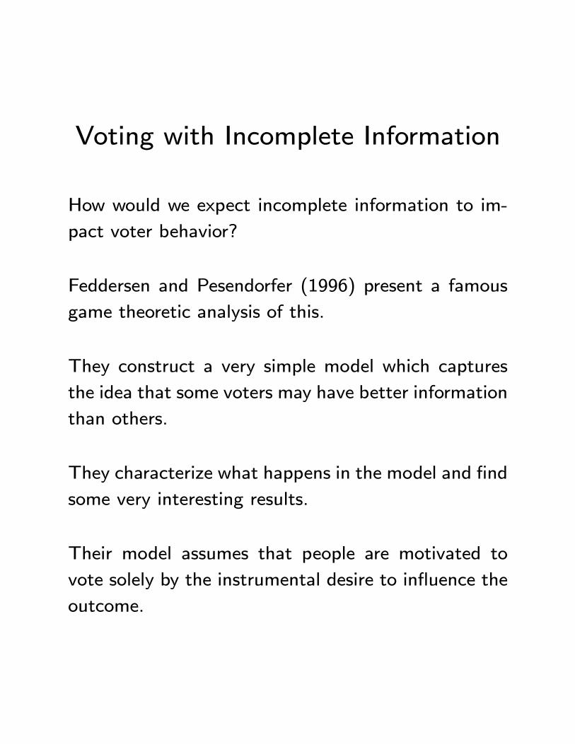
Voting with Incomplete Information

How would we expect incomplete information to im-

pact voter behavior?

Feddersen and Pesendorfer (1996) present a famous

game theoretic analysis of this.

They construct a very simple model which captures

the idea that some voters may have better information

than others.

They characterize what happens in the model and find

some very interesting results.

Their model assumes that people are motivated to

vote solely by the instrumental desire to influence the

outcome.

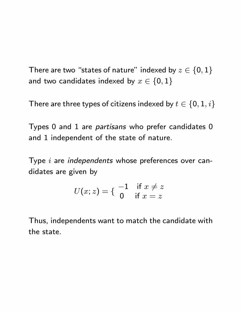
There are two “states of nature” indexed by ∈ {0 1}and two candidates indexed by ∈ {0 1}

There are three types of citizens indexed by ∈ {0 1 }

Types 0 and 1 are partisans who prefer candidates 0

and 1 independent of the state of nature.

Type are independents whose preferences over can-

didates are given by

(; ) = { −1 if 6=

0 if =

Thus, independents want to match the candidate with

the state.

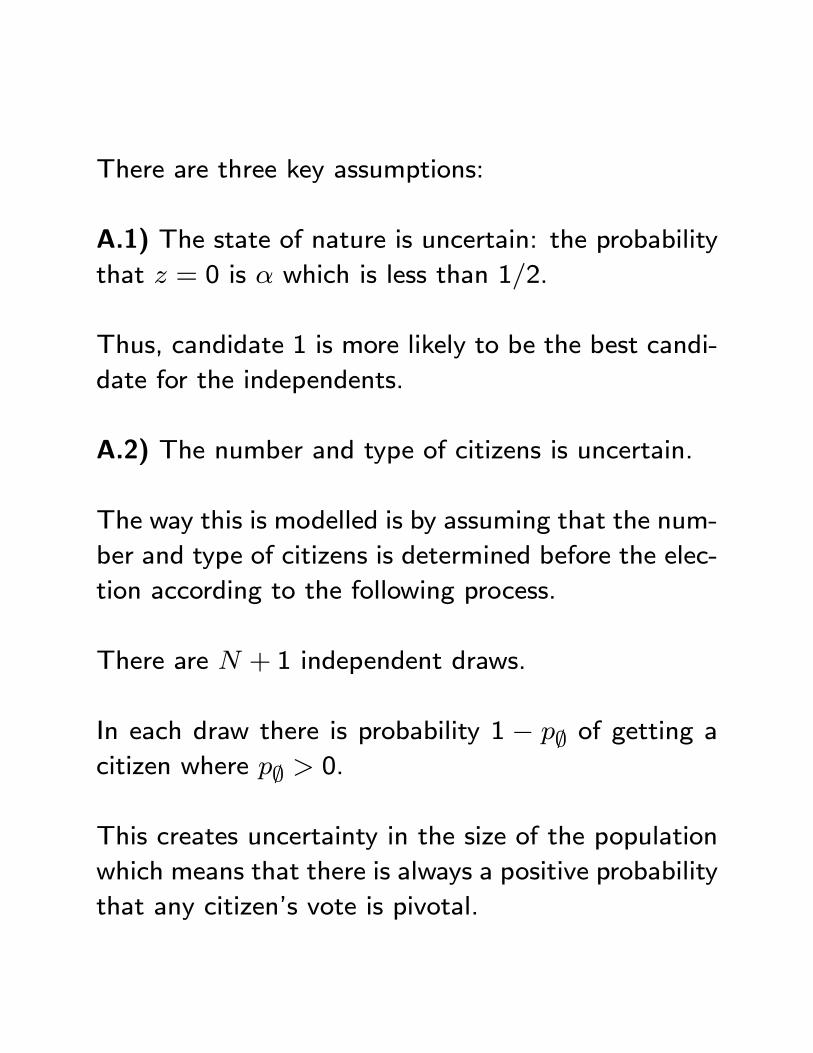
There are three key assumptions:

A.1) The state of nature is uncertain: the probability

that = 0 is which is less than 12.

Thus, candidate 1 is more likely to be the best candi-

date for the independents.

A.2) The number and type of citizens is uncertain.

The way this is modelled is by assuming that the num-

ber and type of citizens is determined before the elec-

tion according to the following process.

There are + 1 independent draws.

In each draw there is probability 1 − ∅ of getting acitizen where ∅ 0.

This creates uncertainty in the size of the population

which means that there is always a positive probability

that any citizen’s vote is pivotal.

Conditional on getting a citizen it is an independent

with probability1−∅, a type 1 partisan with probabil-

ity11−∅, and a type 0 partisan with probability

01−∅..

Thus, , 1, and 0 measure the expected sizes of

the groups in the population.

A.3) Some citizens have more information than oth-

ers.

The way this is modelled is that each citizen receives

a signal ∈ {0 1− 1}.

If a citizen receives signal he knows that Pr{ =1} = .

Thus, if a citizen receives the signal = 1, he knows

that the state is 1.

If he receives the signal = 0, he knows that the state

is 0.

If he receives the signal = 1−, he just knows that

the probability that the state is 0 is .

The probability that a citizen is informed (i.e., ∈{0 1}) is .

Equilibrium

Each citizen chooses one of three actions: abstain,

vote for candidate 0, or vote for candidate 1.

The candidate with the most votes wins and in the

event of a tie, each candidate wins with probability

12.

F & P analyze symmetric Nash equilibria in which all

citizens with type ( ) choose the same strategy

All citizens except the uninformed independents (i.e.,

types ( 1− )) have a strictly dominant strategy.

Partisans vote for their preferred candidate and in-

formed independents vote for the candidate that matches

the state.

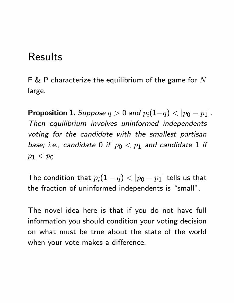
Results

F & P characterize the equilibrium of the game for

large.

Proposition 1. Suppose 0 and (1−) |0 − 1|.Then equilibrium involves uninformed independents

voting for the candidate with the smallest partisan

base; i.e., candidate 0 if 0 1 and candidate 1 if

1 0

The condition that (1− ) |0 − 1| tells us thatthe fraction of uninformed independents is “small”.

The novel idea here is that if you do not have full

information you should condition your voting decision

on what must be true about the state of the world

when your vote makes a difference.

If a candidate has less partisan support but nonethe-

less gets almost as many votes as his opponent he

must be being supported by the informed indepen-

dents.

In this case, he is the best candidate from the view-

point of the uninformed!

Observe that when uninformed independents are vot-

ing for candidate 0 they are voting for the candidate

their own information suggest is likely to be worse.

Thus, they are ignoring their own signals!

Proposition 2. Suppose 0 = 1. Then equilibrium

involves uninformed independents abstaining.

The condition 0 = 1 tells us that the two candidates

have (in expectation) the same sized partisan bases.

In this case, the uninformed independents should just

abstain - thereby delegating the decision to the in-

formed independents.

This is a formal model of “roll off” which we discussed

earlier.

Proposition 3. Suppose 0 and (1−) ≥ |0 − 1|.Then equilibrium involves uninformed independents

mixing between voting for the candidate with the small-

est partisan base and abstaining.

Discussion

The basic insight in the F & P paper is familiar from

optimal bidding behavior in common value auctions.

If you are bidding in an auction and do not have full in-

formation about the object, you should condition your

bid on what must be true about others’ valuations if

your bid is the highest.

If you just bid your signal, you will end up over-paying

for the object if you win it - a result known as the

winner’s curse.

In the voting context, the idea has many interesting

implications.

For example, it suggests that requiring juries to vote

unanimously to convict someone of a crime may lead

people to ignore their private information.

F & P also show that for large the election perfectly

aggregates information in the sense that the outcome

of the election is the same as it would be if all citizens

were perfectly informed.

This is another take on the miracle of aggregation.

The F & P analysis has spawned an experimental lit-

erature which has studies whether the theoretical pre-

dictions are bourne out in the lab.

The “roll-off” prediction of Proposition 2 seems intu-

itive.

The “off-setting voting” prediction described in Propo-

sitions 1 and 2 seems much less intuitive and there is

only mixed support for it.

See Battaglini, Morton, and Palfrey (2010) and Esponda

and Vespa (2011) for conflicting evidence.

I.2 Candidate Behavior

Candidates are citizens who have chosen to run for

elected office.

Candidates have to decide how to campaign.

Once in office, they have to decide how to vote on

legislation and which policy issues to pursue.

Economic theory has largely focused on candidate com-

petition for office.

The objective is to understand the positions that can-

didates will take.

Understanding candidates’ positions is seen as an im-

portant step in understanding the policies that even-

tually emerge from the political process.

We will discuss two candidate competition with Down-

sian and policy-motivated candidates.

We will also discuss the citizen-candidate model and

candidate policy choice with re-election concerns.

I.2.i Two Candidate Competition

We begin with the classic Downsian model of two

candidate electoral competition.

This model is named after Anthony Downs who wrote

a well-known book An Economic Theory of Democ-

racy in the 1950s.

In this model, two candidates whose objective is to win

office compete by staking out ideological positions in

a one dimensional space.

A) The Downsian Model

There are two candidates, and

Each candidate ∈ {} must choose an ideology ∈ [0 1] on which to run

The interpretation is that 0 is the most extreme left-

wing ideology and 1 the most extreme right-wing ide-

ology

This one dimensional notion of ideology is quite nat-

ural, since it is commonplace to talk of candidates as

being centrist, extreme right, moderate right, etc.

The notion of choosing ideology is also natural, since

it is commonplace to talk of candidates moving to the

center, appealing to the base, etc.

If elected, candidates are assumed to pursue policies

consistent with the ideology they have run on in the

election.

Citizens have ideologies distributed over the interval

[0 1].

Let () be the fraction of voters with ideology ≤ .

Assume (0) = 0, and 0.

Let denote the ideology of the median voter ; that

is, the voter exactly in the middle of the ideology dis-

tribution.

Formally, is defined by () = 12.

A voter with ideology obtains utility ( ; ) if can-

didate is elected.

The utility function ( ; ) is assumed to satisfy the

single-crossing property.

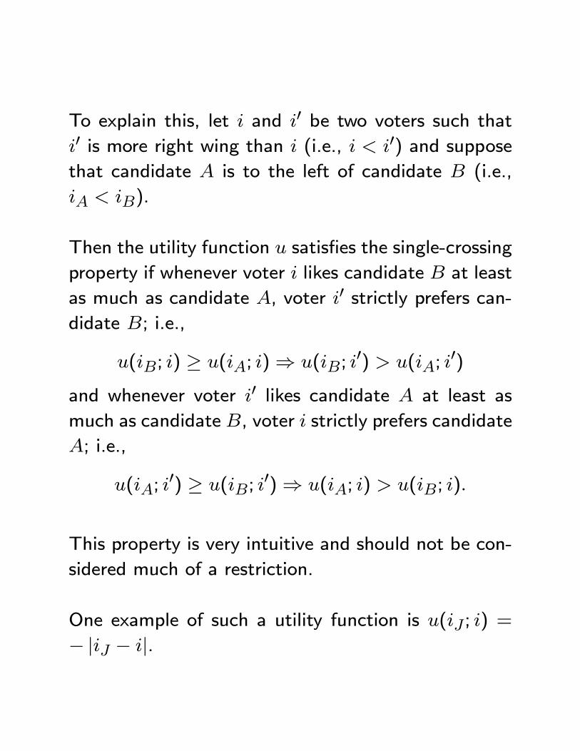
To explain this, let and 0 be two voters such that0 is more right wing than (i.e., 0) and supposethat candidate is to the left of candidate (i.e.,

).

Then the utility function satisfies the single-crossing

property if whenever voter likes candidate at least

as much as candidate , voter 0 strictly prefers can-didate ; i.e.,

(; ) ≥ (; )⇒ (; 0) (;

0)

and whenever voter 0 likes candidate at least as

much as candidate , voter strictly prefers candidate

; i.e.,

(; 0) ≥ (;

0)⇒ (; ) (; )

This property is very intuitive and should not be con-

sidered much of a restriction.

One example of such a utility function is ( ; ) =

− | − |.

When voters have these utility functions they are said

to have distance preferences.

Another example is ( ; ) = − ( − )2.

When voters have these utility functions they are said

to have quadratic preferences.

Candidates get a payoff 0 if they win and 0 oth-

erwise.

Thus, candidates have no ideological preferences and

are purely office motivated ; i.e., they just want to win.

Each candidate simultaneously announces his ide-

ology ∈ [0 1]

Each voter votes for the candidate whose ideology he

prefers.

If a voter is indifferent he votes for each candidate

with equal probability.

The candidate with the most votes is elected and pur-

sues policies consistent with his announced ideology.

If each candidate has the same number of votes, then

the election is decided by the toss of a fair coin.

Equilibrium

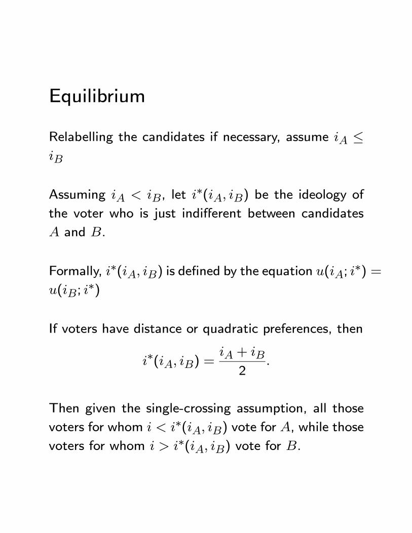
Relabelling the candidates if necessary, assume ≤

Assuming , let ∗( ) be the ideology of

the voter who is just indifferent between candidates

and .

Formally, ∗( ) is defined by the equation (; ∗) =(;

∗)

If voters have distance or quadratic preferences, then

∗( ) = +

2

Then given the single-crossing assumption, all those

voters for whom ∗( ) vote for , while thosevoters for whom ∗( ) vote for .

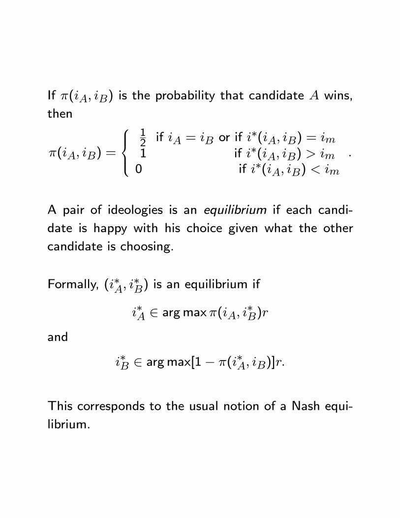
If ( ) is the probability that candidate wins,

then

( ) =

⎧⎪⎨⎪⎩12if = or if ∗( ) =

1 if ∗( ) 0 if ∗( )

A pair of ideologies is an equilibrium if each candi-

date is happy with his choice given what the other

candidate is choosing.

Formally, (∗ ∗) is an equilibrium if

∗ ∈ argmax( ∗)and

∗ ∈ argmax[1− (∗ )]

This corresponds to the usual notion of a Nash equi-

librium.

Results

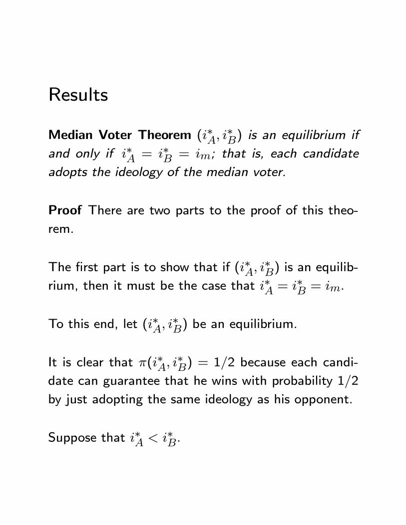
Median Voter Theorem (∗ ∗) is an equilibrium if

and only if ∗ = ∗ = ; that is, each candidate

adopts the ideology of the median voter.

Proof There are two parts to the proof of this theo-

rem.

The first part is to show that if (∗ ∗) is an equilib-

rium, then it must be the case that ∗ = ∗ = .

To this end, let (∗ ∗) be an equilibrium.

It is clear that (∗ ∗) = 12 because each candi-

date can guarantee that he wins with probability 12

by just adopting the same ideology as his opponent.

Suppose that ∗ ∗.

Then, it follows from the fact that (∗ ∗) = 12

that the median voter must be indifferent between the

two candidates; i.e., that ∗(∗ ∗) = .

But now imagine that candidate deviates from the

equilibrium by proposing the median voter’s ideology.

Then, the median voter strictly favors and hence

∗( ∗) .

It follows that ( ∗) = 1 implying that would

win with probability 1 - which contradicts the fact that

(∗ ∗) is an equilibrium.

Thus, we conclude it must be the case that ∗ = ∗.

If ∗ = ∗ 6= then either ∗ = ∗ or ∗ =

∗ .

Consider only the former case, since the latter is sim-

ilar.

If ∗ = ∗ candidate could deviate by moving

his position to .

Then, ∗(∗ ) implying that (∗ ) = 0.

This means that candidate would win with proba-

bility 1 - which contradicts the fact that (∗ ∗) is an

equilibrium.

This completes the proof of the first part.

The second part of the proof is to show that if ∗ =∗ = then (∗

∗) is an equilibrium.

This follows from the fact that any candidate who

deviated from would lose and hence reduce his

expected payoff. QED

Substantively, this model predicts that competition

leads candidates to move to the political center.

In terms of policy, the result suggests that policies in

a representative democracy will be those that would

be preferred by middle of the road voters.

Empirical Evidence

There have been many attempts to test the Median

Voter Theorem.

One of the most convincing is the effort by Gerber

and Lewis in the 2004 Journal of Political Economy.

They use voting data from Los Angeles County to

estimate the distribution of voter ideologies district

by district.

In particular, they have votes on both ballot proposi-

tions and candidate elections which allows them to do

a convincing job of estimating voter ideologies.

They then estimate the ideology of the winning can-

didates from legislator voting records.

They look at U.S. House and California Assembly

races.

They find little support for the idea that the ideology

of winning candidates should match the ideology of

the median voter in their constituency.

In particular, the ideology of winning candidates can

diverge significantly from the median voter’s ideology

in heterogeneous districts (i.e., districts with a lot of

variance in citizen ideologies).

Winning Republicans are to the right of the median

voter in their district, while winning Democrats are to

the left.

This is consistent with casual empiricism and the find-

ings of most who have looked carefully at the issue.

The one exception is a recent paper by Ferreira and

Gyourko in the 2010 Quarterly Journal of Economics.

They compare policies in cities with Republican and

Democrat mayors.

They use a regression discontinuity design which com-

pares policies in cities which elected a Democrat mayor

by a very small margin with those who elected a Re-

publican mayor by a very small margin.

The idea behind this research design is that these two

groups of cities should be basically quite similar, ex-

cept for the partisan affiliation of the mayor.

If the Median Voter Theorem is right, both Democrat

and Republican mayors should implement basically the

same policies.

This means that there should be no difference between

the policies in these two groups of cities, which is what

they find.

B) Policy-motivated Candidates

The Downsian assumption that candidates are purely

office-motivated is strange.

Indeed, it is logically inconsistent because candidates

must be citizens and citizens are presumed to have

policy preferences.

What would happen if we modified the Downsian model

by assuming that the two candidates and had,

respectively, utility functions ( ; ) and ( ; )

with “true” ideologies and where

?

In fact, it can be shown that the Median Voter The-

orem is robust to this extension.

However, if candidates face uncertainty in the loca-

tion of the median voter, their policy preferences do

matter.

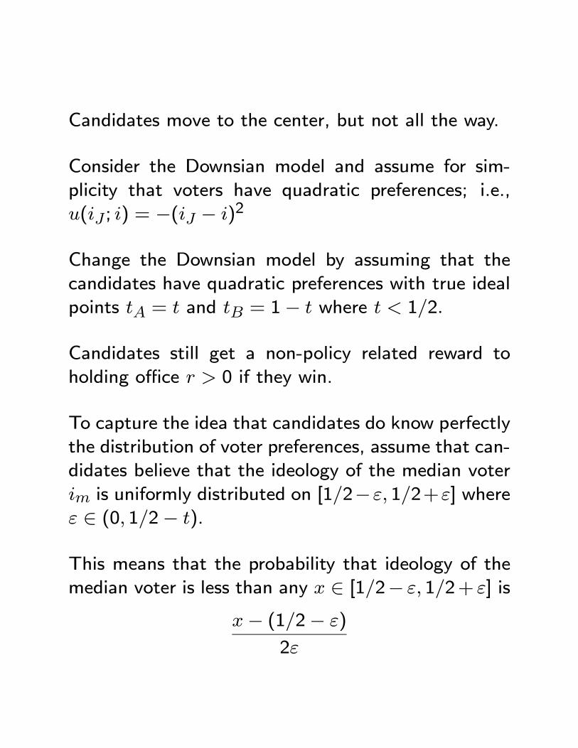
Candidates move to the center, but not all the way.

Consider the Downsian model and assume for sim-

plicity that voters have quadratic preferences; i.e.,

( ; ) = −( − )2

Change the Downsian model by assuming that the

candidates have quadratic preferences with true ideal

points = and = 1− where 12

Candidates still get a non-policy related reward to

holding office 0 if they win.

To capture the idea that candidates do know perfectly

the distribution of voter preferences, assume that can-

didates believe that the ideology of the median voter

is uniformly distributed on [12− 12+] where

∈ (0 12− ).

This means that the probability that ideology of the

median voter is less than any ∈ [12− 12+ ] is

− (12− )

2

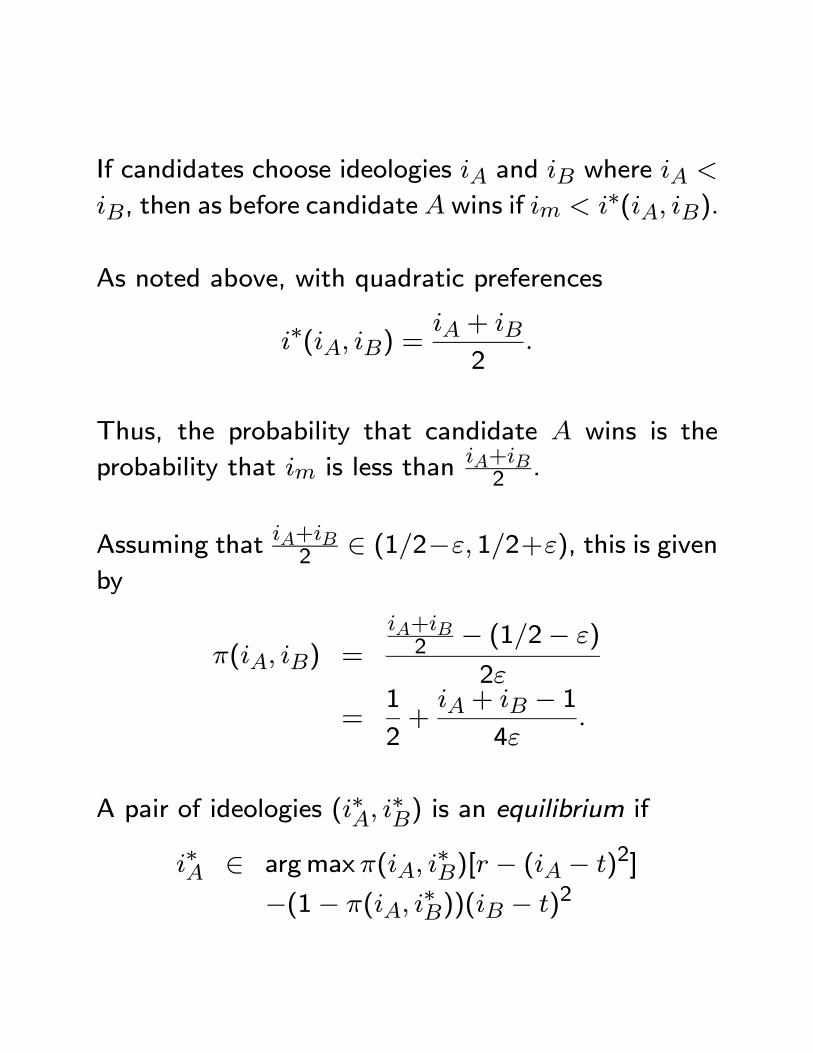
If candidates choose ideologies and where

, then as before candidate wins if ∗( ).

As noted above, with quadratic preferences

∗( ) = +

2

Thus, the probability that candidate wins is the

probability that is less than+2

.

Assuming that+2

∈ (12− 12+), this is givenby

( ) =

+2

− (12− )

2

=1

2+ + − 1

4

A pair of ideologies (∗ ∗) is an equilibrium if

∗ ∈ argmax( ∗)[ − ( − )2]

−(1− ( ∗))( − )2

and

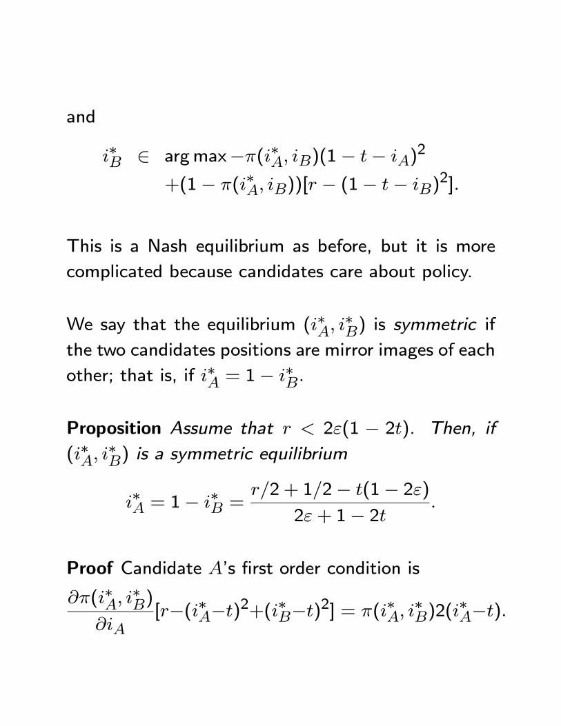
∗ ∈ argmax−(∗ )(1− − )2

+(1− (∗ ))[ − (1− − )2]

This is a Nash equilibrium as before, but it is more

complicated because candidates care about policy.

We say that the equilibrium (∗ ∗) is symmetric if

the two candidates positions are mirror images of each

other; that is, if ∗ = 1− ∗.

Proposition Assume that 2(1 − 2). Then, if(∗

∗) is a symmetric equilibrium

∗ = 1− ∗ =2 + 12− (1− 2)

2+ 1− 2

Proof Candidate ’s first order condition is

(∗ ∗)

[−(∗−)2+(∗−)2] = (∗

∗)2(

∗−)

Using the expression for (∗ ∗) and the fact that

the equilibrium is symmetric, this implies that

1

4[ − (∗ − )2 + (∗ − )2] = (∗ − )

Using the fact that ∗ = 1 − ∗, we can rewrite thisas:

1

4[ − (∗ − )2 + (1− ∗ − )2] = (∗ − )

Expanding this, yields

1

4[ + 4∗+ 1− 2∗ − 2] = (∗ − )

We can solve this equation for ∗ yielding

∗ =2+ 12− (1− 2)

2+ 1− 2

QED

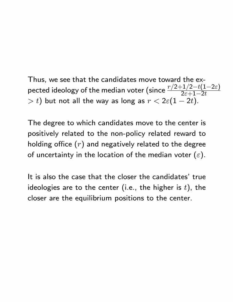
Thus, we see that the candidates move toward the ex-

pected ideology of the median voter (since2+12−(1−2)

2+1−2 ) but not all the way as long as 2(1− 2).

The degree to which candidates move to the center is

positively related to the non-policy related reward to

holding office () and negatively related to the degree

of uncertainty in the location of the median voter ().

It is also the case that the closer the candidates’ true

ideologies are to the center (i.e., the higher is ), the

closer are the equilibrium positions to the center.

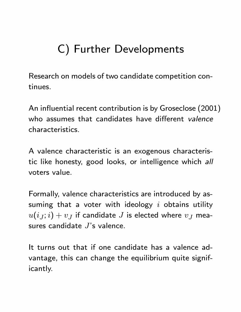
C) Further Developments

Research on models of two candidate competition con-

tinues.

An influential recent contribution is by Groseclose (2001)

who assumes that candidates have different valence

characteristics.

A valence characteristic is an exogenous characteris-

tic like honesty, good looks, or intelligence which all

voters value.

Formally, valence characteristics are introduced by as-

suming that a voter with ideology obtains utility

( ; ) + if candidate is elected where mea-

sures candidate ’s valence.

It turns out that if one candidate has a valence ad-

vantage, this can change the equilibrium quite signif-

icantly.

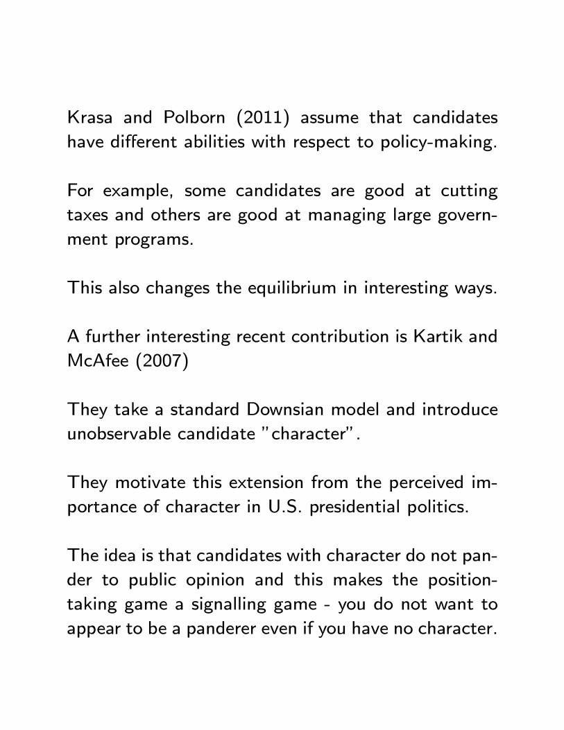
Krasa and Polborn (2011) assume that candidates

have different abilities with respect to policy-making.

For example, some candidates are good at cutting

taxes and others are good at managing large govern-

ment programs.

This also changes the equilibrium in interesting ways.

A further interesting recent contribution is Kartik and

McAfee (2007)

They take a standard Downsian model and introduce

unobservable candidate ”character”.

They motivate this extension from the perceived im-

portance of character in U.S. presidential politics.

The idea is that candidates with character do not pan-

der to public opinion and this makes the position-

taking game a signalling game - you do not want to

appear to be a panderer even if you have no character.

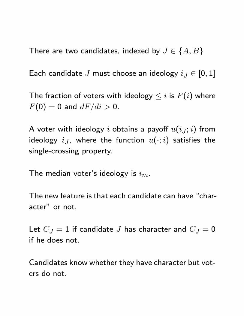
There are two candidates, indexed by ∈ {}

Each candidate must choose an ideology ∈ [0 1]

The fraction of voters with ideology ≤ is () where

(0) = 0 and 0.

A voter with ideology obtains a payoff ( ; ) from

ideology , where the function (·; ) satisfies thesingle-crossing property.

The median voter’s ideology is .

The new feature is that each candidate can have “char-

acter” or not.

Let = 1 if candidate has character and = 0

if he does not.

Candidates know whether they have character but vot-

ers do not.

All they know is that the probability that = 1 is

∈ (0 1).

If a candidate has character his ideology choice is

non-strategic - it is the realization of a random vari-

able with CDF () and density ().

This formalizes the idea that candidates with charac-

ter do not pander.

If a candidate does not have character then he chooses

strategically in the usual way; i.e., he seeks to max-

imize the probability of winning.

Voters obtain an additional benefit from electing

a candidate with character (why this is, is not mod-

elled).

Because of this, candidates without character would

like to signal they have character.

If they just choose the median voter’s ideology then

voters will conclude that they do not have character.

Thus, their position choice becomes a signal and a

signalling game results.

Equilibrium

If candidate does not have character his strategy is

described by (); i.e., () is the probability he

chooses an ideology less than .

If candidate has character his strategy is just ().

At the time of voting, voters are not sure whether

each candidate has character.

Let Φ() represent voters’ beliefs concerning the prob-

ability that candidate has character given he selects

position .

A symmetric equilibrium consists of a candidate strat-

egy () and voter beliefs Φ() such that: i) the strat-

egy is optimal for the candidates given the voting be-

havior implied by the voters’ beliefs, and ii) the voters’

beliefs are rational given the candidate strategy.

Proposition. In equilibrium, strategic candidates mix

over positions. In particular, the probability that they

choose is zero. Moreover, i) candidates without

character win with a higher probability than candi-

dates with character; ii) voters’ posterior belief on

character is single-troughed around the median; that

is, Φ() is decreasing for and increasing for

; iii) as goes to ∞, () converges to ();

and iv) as goes to 0, () converges to the distrib-

ution that puts point mass on .

The paper is interesting in that it identifies an impor-

tant reason why even the most cynical candidates will

not pander totally to the median voter.

However, it does not explain why voters value candi-

dates with “character” or why candidates with char-

acter would wish to ignore voters’ preferences.

If you are interested in this aspect of the argument

see the paper by Callander (2008).

I.2.ii The Citizen-Candidate Approach

Once we recognize that candidates have policy pref-

erences, we must address the question of what deter-

mines these preferences.

Thus, in the model just considered what determines

and ?

To understand this, we have to consider the decision

of citizens of whether to run for office.

This also raises the question of the number of candi-

dates who decide to run.

The citizen-candidate model seeks to explain the num-

ber of candidates running and their policy preferences.

In so doing, it offers a very different vision of candidate

behavior: the key assumption of the approach is that

candidates must run on their true ideologies.

There are two distinct justifications for this assump-

tion.

First, candidates may prefer to be honest and there-

fore find it costly to misrepresent their true beliefs.

Second, once elected, candidates’ behavior may plau-

sibly be driven more by their true ideologies than the

ideologies they announce in the campaign.

If this is the case, voters will recognize that what mat-

ters for predicting policy choices will be what the can-

didate truly believes rather than what he annouces.

The assumption that candidates must run on their

true ideologies is fundamentally different than that

underlying the prior models which assume candidates

can reposition themselves at will.

Casual empiricism seems to suggest that there is some

truth to both positions.

Candidates certainly sometimes seem to change their

positions (i.e., to flip-flop) and some voters seem to

believe them (e.g., Mitt Romney’s conversion to a

social conservative).

However, the controversy which arises following a flip-

flop certainly suggests that voters feel that candidates

ought to present their true policy preferences.

There is some empirical work that is relevant to this

discussion (see, for example, Lee, Morretti, and Butler

(2004)).

In support of the citizen-candidate model, it does not

seem to be the case that legislators change their po-

sitions (as measured by voting records) when their

constituency changes (say, via redistricting).

Moreover, survey evidence suggests that repositioning

leads voters to distrust candidates’ announced posi-

tions and their integrity.

The Model

The citizen-candidate approach models elections as a

three stage game.

In Stage 1, citizens decide whether or not to enter the

race as a candidate.

Running entails a sunk cost which may be thought of

as the time devoted to running a campaign.

In Stage 2, citizens vote over the set of self-declared

candidates.

Voting is assumed not to be costly, so everybody

votes.

Voting is strategic in some treatments of the model

and sincere in others.

In Stage 3, the candidate with the most votes is elected

(plurality rule) and follows his/her true ideology when

in office.

If there is a tie, the winning candidate is determined

by the toss of a fair coin.

When voting in Stage 2, citizens rationally anticipate

that the winning candidate will follow his/her true

ideology and this determines their payoffs from the

different candidates.

Importantly, citizens are assumed to know each can-

didate’s true ideology.

In Stage 1, candidates are assumed to perfectly an-

ticipate how citizens will vote for any given set of

candidates.

Roughly speaking, an equilibrium is a set of candi-

dates such that, given perfect anticipation of voting

behavior, every citizen who is a candidate is better off

being in the race given who else is in the race and

every citizen who is not a candidate is better off not

in the race.

Results

The advantage of the citizen-candidate model is that

it endogenizes the number of candidates and their pol-

icy positions.

The disadvantage of the model is that it does not yield

a unique prediction.

There are many different possible equilibria, some in-

volving spoiler candidates who run just to prevent

other candidates from winning.

We will just look at the predictions of the model con-

cerning equilibria with two candidates.

This will enable us to compare predictions with the

previous models.

To facilitate comparisons, lets assume the usual set-

up in which citizens have ideologies distributed over

the interval [0 1] and utility functions satisfying single

crossing.

Assume that running for office entails a cost and

that the winning candidate gets a non-policy related

benefit of holding office .

First assume that citizens vote sincerely (as in Os-

borne and Slivinski (1996)).

Two candidates with ideologies and running

against each other is an equilibrium if (i) candidates

and want to run against each other and (ii) there

is no third candidate who would gain from entering

the race.

The first prediction of the model is that and will

be on opposite sides of the median voter’s ideology

and the median voter will be indifferent between the

two candidates; i.e., and (; ) =

(; )

The reason for this is that both candidates must stand

a chance of winning.

This is because if a candidate knew he was going to

lose, he would be better off dropping out of the race

and saving the cost of running.

The model also predicts that the ideologies of the two

candidates can neither be too far apart nor too close

together.

The ideologies cannot be too far apart, otherwise a

centrist candidate will be able to enter and win the

race.

For example, if citizens have quadratic preferences, a

candidate with ideology who entered would obtain

a vote share

( +

2)− (

+

2)

Assuming − is small, this vote share must be less

than

max{ ( +

2) 1− (

+

2)}

otherwise such a median candidate would enter.

This limits how far apart and can be.

The ideologies cannot be too close together because if

they were, one candidate would be better off dropping

out and letting the other candidate be elected (since

).

For example, with quadratic preferences, it must be

the case that

1

2( − )

2 −

2

The basic picture in terms of the positions of the can-

didates looks very similar to the predictions of the

candidate competition model with policy preferences

and voter uncertainty.

If we assume strategic voting (as in Besley and Coate

(1997)), it is no longer the case that the candidates

cannot be too far apart.

With strategic voting even if the two candidates are

at the extremes, a centrist candidate would not nec-

essarily be able to enter and win.

The reason is that in a three way race, centrist vot-

ers might continue to view the race as a contest be-

tween the two extremist candidates and be reluctant

to switch their votes to the centrist candidate for fear

of “wasting their votes”.

This result is notable because it shows that extremism

can arise even with a very competitive looking political

system.

I.2.iii Candidate Policy Choice withRe-election Concerns

In the citizen-candidate approach, candidates can make

no policy commitments in the campaign.

They cannot credibly commit to do anything other

than maximize their true policy preferences when elected.

However, this analysis is purely static and it seems

reasonable that even if campaign promises are non-

credible, the threat of re-election might effectively

constrain politicians’ choices when in office.

This brings us to political agency models which study

the choices of politicians facing the threat of re-election.

In these models, the politician is the agent and the

voters are the principals.

The maintained hypothesis is that the politician’s pref-

erences (may) differ from that of the voters.

These models differ from standard principal-agent mod-

els in that the principals have only a very crude incen-

tive structure - they can either re-elect the politician

or remove him from office.

There are two strands of work in the political agency

tradition.

Early papers assumed that politicians were all identical

and that voters used retrospective voting to discipline

them.

Thus, voters view all politicians as equally good or

bad, but, in a conscious effort to provide discipline,

remove underperforming candidates from office.

Later work assumes that politicians are different and

that voters use forward-looking voting rules when de-

ciding to re-elect them; i.e., they vote for the incum-

bent if and only if they believe he is a better candidate

than the challenger

In the first class of models, incentives for politicians

are explicit.

Politicians know that they will not be re-elected unless

they perform above a certain standard.

In the second class, incentives are implicit.

Politicians know that they will not be re-elected if they

are viewed as less attractive than their challengers.

But they can manipulate voters’ beliefs about their

characteristics (preferences and/or capabilities) via their

performance.

The second class of models are basically signalling

models and are a little harder to work with than the

first class.

Nonetheless, the assumption that all politicians are

the same is unappealing.

Moreover, casual empiricism suggests that politicians

care greatly about their reputations with voters and

this influences their choices (votes on bills, decisions

as to which policy issues to pursue, etc).

These factors have made the second class of political

agency models more popular and they are now used

quite widely in political science.

We will consider the paper by Banks and Sundaram

(1998) which nicely illustrates the logic of this second

class of models.

See Ferejohn (1986) for a nice example of the first

class of models.

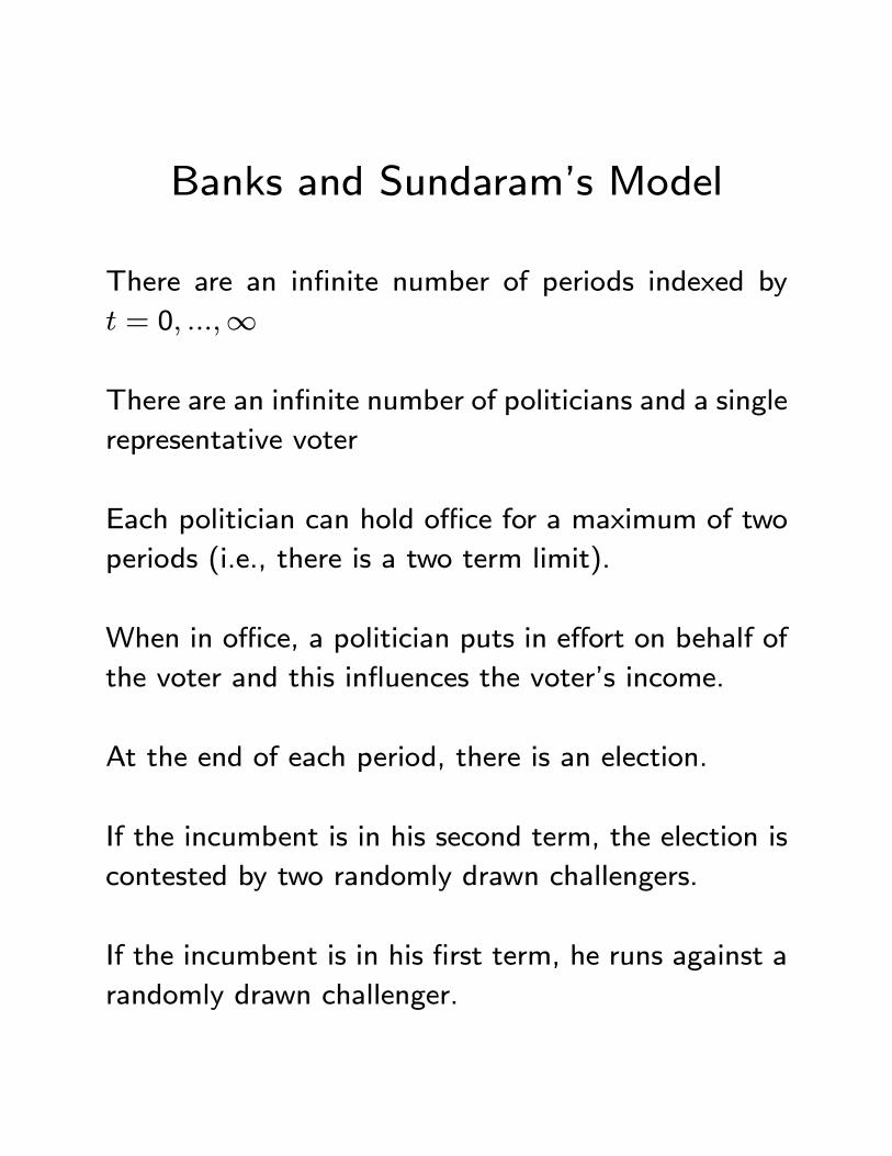
Banks and Sundaram’s Model

There are an infinite number of periods indexed by

= 0 ∞

There are an infinite number of politicians and a single

representative voter

Each politician can hold office for a maximum of two

periods (i.e., there is a two term limit).

When in office, a politician puts in effort on behalf of

the voter and this influences the voter’s income.

At the end of each period, there is an election.

If the incumbent is in his second term, the election is

contested by two randomly drawn challengers.

If the incumbent is in his first term, he runs against a

randomly drawn challenger.

If a first term incumbent fails to be re-elected, he

cannot run again.

Politicians come in different “types”.

The possible politician types are {1 } where1 .

Higher types like to work harder on behalf of the voter,

so 1 is the worst type and the best.

The fraction of type politicians in the population

is 0.

In any period , the incumbent chooses some effort

level ∈ [min max].

This effort determines stochastically the voter’s in-

come .

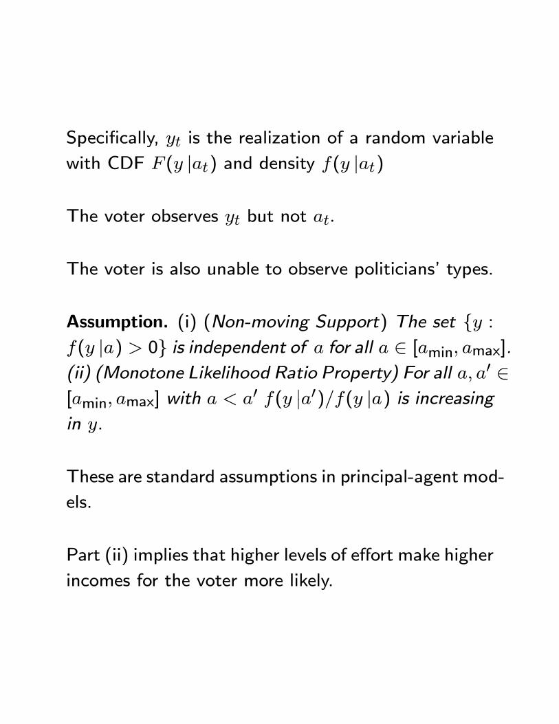
Specifically, is the realization of a random variable

with CDF ( |) and density ( |)

The voter observes but not

The voter is also unable to observe politicians’ types.

Assumption. (i) (Non-moving Support) The set { :( |) 0} is independent of for all ∈ [min max].(ii) (Monotone Likelihood Ratio Property) For all 0 ∈[min max] with 0 (

¯̄0)( |) is increasing

in .

These are standard assumptions in principal-agent mod-

els.

Part (ii) implies that higher levels of effort make higher

incomes for the voter more likely.

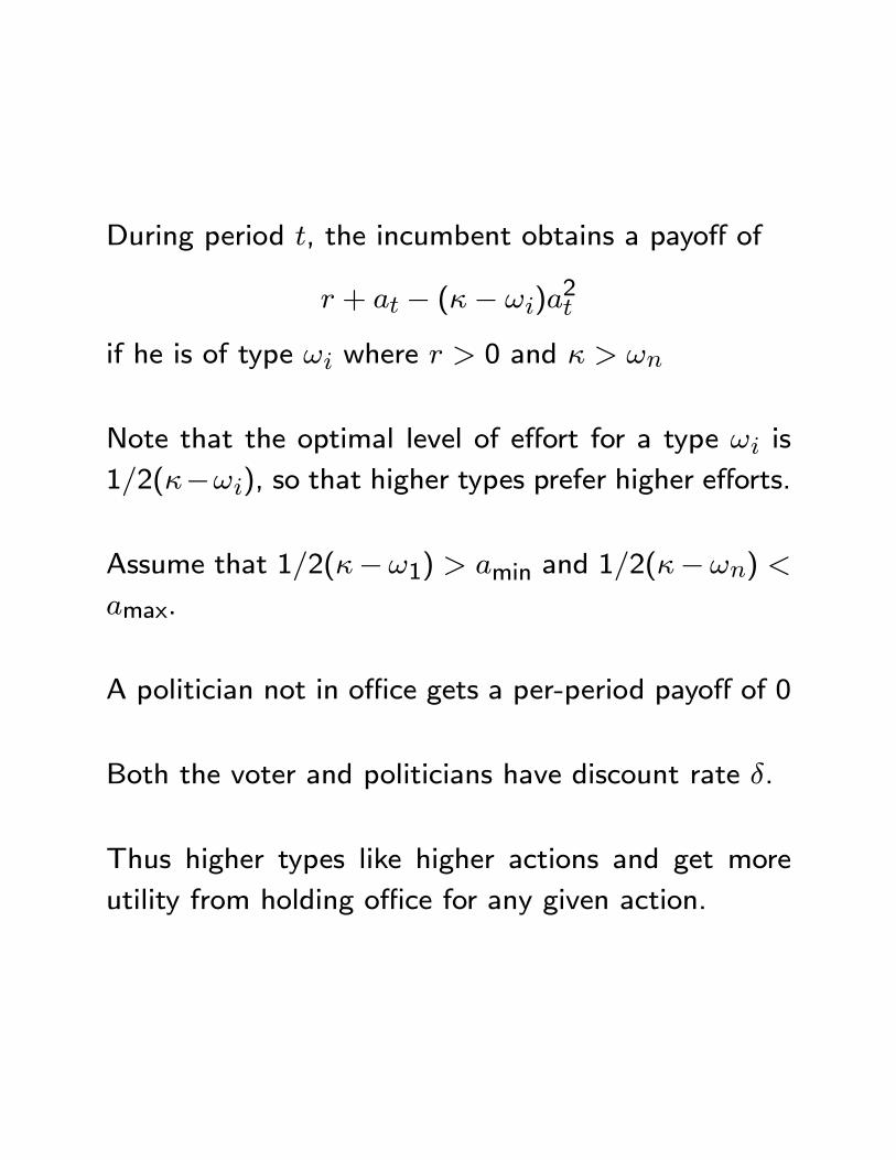
During period , the incumbent obtains a payoff of

+ − (− )2

if he is of type where 0 and

Note that the optimal level of effort for a type is

12(−), so that higher types prefer higher efforts.

Assume that 12(−1) min and 12(−)

max.

A politician not in office gets a per-period payoff of 0

Both the voter and politicians have discount rate .

Thus higher types like higher actions and get more

utility from holding office for any given action.

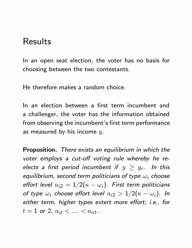
Results

In an open seat election, the voter has no basis for

choosing between the two contestants.

He therefore makes a random choice.

In an election between a first term incumbent and

a challenger, the voter has the information obtained

from observing the incumbent’s first term performance

as measured by his income .

Proposition. There exists an equilibrium in which the

voter employs a cut-off voting rule whereby he re-

elects a first period incumbent if ≥ . In this

equilibrium, second term politicians of type choose

effort level 2 = 12( − ). First term politicians

of type choose effort level 1 12( − ). In

either term, higher types extert more effort; i.e., for

= 1 or 2, .

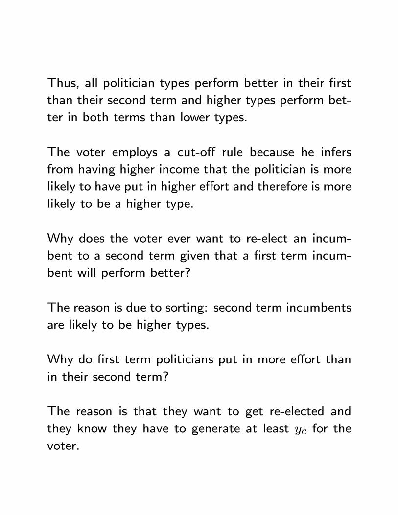
Thus, all politician types perform better in their first

than their second term and higher types perform bet-

ter in both terms than lower types.

The voter employs a cut-off rule because he infers

from having higher income that the politician is more

likely to have put in higher effort and therefore is more

likely to be a higher type.

Why does the voter ever want to re-elect an incum-

bent to a second term given that a first term incum-

bent will perform better?

The reason is due to sorting: second term incumbents

are likely to be higher types.

Why do first term politicians put in more effort than

in their second term?

The reason is that they want to get re-elected and

they know they have to generate at least for the

voter.

This provides an incentive which is absent in their

second term.

In essence, first term politicians are trying to create a

good reputation for themselves.

Empirical Evidence

This model predicts a term limit effect: politicians

behave differently when they can and cannot run for

for re-election.

This raises the empirical question of whether politi-

cians do indeed behave differently in their last terms.

One interesting study is that by Besley and Case in

the 1995 Quarterly Journal of Economics.

They exploit the fact that in almost half the U.S.

states, governors face a binding term limit.

They find that when governors are in their last term,

state taxes and spending are higher.

This suggests that in their early terms, governors are

trying to signal that they are more fiscally conservative

then they actually are.

I.3 Legislatures

In almost all practical applications, policy is made by

a legislature of elected representatives.

There is a large literature on legislative decision mak-

ing.

This literature focuses on trying to predict the policies

that would be selected by a majority rule legislature

composed of legislators who disagree on what the op-

timal policy should be.

Legislators’ are assumed to have different policy pref-

erences because they are elected by different districts.

Legislative Decision-Making Model

Consider a legislature consisting of legislators in-

dexed by = 1 .

Assume is odd and ≥ 3 and suppose that the legis-lature operates by majority rule.

Suppose the legislators have to choose some policy

from some set of alternative policies .

Legislator ’s utility if policy is selected is ().

This utility function will reflect both the legislator’s

ideology and also how the policy will impact him and

his constituents.

What policy would we expect the legislature to choose?

Condorcet Winners

A policy ∗ ∈ is said to be a Condorcet Winner if

it would defeat or tie any other policy in a pairwise

majority vote.

Assuming that legislators abstain if they are indifferent

between alternatives, this requires that for any policy

∈ the number of legislators who prefer ∗ to isat least as large as the number who prefer to ∗.

Formally, the requirement is that for all ∈

#{ |(∗) ()} ≥ #{ |() (∗)}

If a unique Condorcet winner exists, it is reasonable

to think that the legislature would select it.

After all, for any other policy, there will exist another

policy that could be proposed that would defeat it.

Thus, if the legislature were about to implement that

policy, a legislator could offer an amendment propos-

ing a majority-preferred policy and we might expect

that amendment to be supported.

So will a Condorcet winner exist?

This depends on the nature of the set of alternative

policies and the legislators’ utility functions.

Example 1

Suppose that the legislature is making a discrete de-

cision, such as whether to declare war or not.

The set of policy alternatives then just consists of two

elements and where, say, means declare war and

means not declare war.

In this case, there will always exist a Condorcet winner

- it is just whichever option is favored by the majority

of legislators.

Example 2

Suppose that the legislators are choosing the aggre-

gate level of spending for a particular department (e.g.,

defense).

Then the set of alternative policies will be = { : ≥ 0}

In this case, there are an infinite number of policy

alternatives.

Let legislator ’s ideal spending level be ∗ ; that is,

∗ = argmax{() : ≥ 0}

Label the legislators such that

∗1 ∗

Presumably, if the policy is defense spending, left wing

Democrats will prefer a smaller level and conservative

Republicans a higher level.

Thus, for a policy issue like this, legislators’ preferred

positions will reflect their underlying ideologies.

Let denote the median legislator ; that is, the leg-

islator such that as many legislators prefer a lower as

prefer a higher spending level.

Suppose that the legislators’ utility functions satisfy

the single-crossing property.

Thus, if and 0 are two legislators such that 0 prefersmore spending than (i.e., 0) and spending level is smaller than 0, then

(0) ≥ ()⇒ 0(

0) 0()

and

0() ≥ 0(0)⇒ () (

0)

Proposition In Example 2, the policy preferred by the

median legislator is a Condorcet winner.

Example 3

Suppose that the legislators are dividing up a fixed

budget between projects located in the legislators’ dis-

tricts.

Then a policy is a vector (1 ) where is the

spending in legislator ’s district.

The set of alternative policies is

= {(1 ) ∈ <+ :X=1

= }

where denotes the budget.

It may be reasonable to assume that

(1 ) =

Thus, each legislator would prefer that all the projects

are located in his own district.

This is an example of a so-called distributive policy -

the policy issue involves distributing a benefit between

different constituencies.

For such issues, ideology is less important than how

the policy impacts a legislator’s district.

In this example, there are not only an infinite number

of policy alternatives as in Example 2 but set of policy

alternatives is multi- as opposed to uni-dimensional.

Proposition In Example 3, there exists no Condorcet

winner.

Proof Let (1 ) ∈ .

Assume by relabeling as necessary that 1 0.

Then (01 0) = (0 2+1−1 +

1−1) is pre-

ferred by legislators 2 through to (1 ).

QED

Discussion

The non-existence of a Condorcet winner arising in

Example 3 is a general phenomenon.

Whenever we are looking at distributive policies (or

any other multi-dimensional policies), we are very likely

to run into this type of problem.

There is a large literature that establishes this (for

discussion and analysis see, for example, McKelvey

(1976)).

This means that while looking for a Condorcet winner

is a natural thing to do, it is often not going to deliver

a prediction.

This is an interesting result in its own right since it

suggests that in many situations the notion of the

“will of the majority” is not really well-defined.

One approach to making predictions for distributive

policy problems like those in Example 3, is to build

more structured models of how the legislators interact.

Thus, we need to specify which legislators get to make

policy proposals, when voting takes place, etc.

The structure will “induce” an equilibrium leading to

the idea of structure-induced equilibrium (Shepsle).

Example 3 Revisited

To illustrate, lets go back to Example 3 and make

some assumptions about how decision-making takes

place.

Assume at the beginning of the legislative session, one

legislator is selected to make a policy proposal.

Such a proposal would be a proposed division of the

budget (1 )

All legislators then vote for or against the proposal.

If a majority of legislators vote for the proposal, it is

implemented, and the legislators move on to deal with

some other policy issue.

If a majority of legislators vote against the proposal,

another legislator is selected to make a policy pro-

posal.

All legislators then vote for or against this proposal

and if a majority vote for it is implemented.

If a majority of legislators vote against the proposal,

another legislator is selected to make a policy pro-

posal, etc, etc.

This process continues until a proposal is passed.

It is natural to assume that the legislators would rather

pass a proposal sooner rather than later.

To capture this, assume that if the policy (1 )

is agreed to after proposal rounds, legislator obtains

utility −1, where 1.

What would happen under these rules?

Much will depend on the rule for selecting proposers.

The simplest case to analyze is when each legislator

is equally likely to be chosen.

Thus, in each proposal round, each legislator is se-

lected to be proposer with probability 1.

Under this proposer selection rule, we can figure out

what might happen.

Equilibrium in Example 3

The structure we have described gives rise to a game

between the legislators.

The game is similar to the alternating offer bargaining

model used in economics.

The differences are that there are more than two play-

ers and majority agreement is required instead of unan-

imous agreement.

The game is referred to as a legislative bargaining

game (Baron and Ferejohn (1989)).

A strategy for a legislator describes the proposal that

he will make if selected and how will he vote on any

proposal.

In principle, strategies may depend in complicated

ways on the entire history of play.

We restrict attention to stationary strategies which

do not depend on the proposal round or the history of

play.

This rules out strategies whereby a proposing legis-

lator discriminates against legislators who have previ-

ously proposed and offered his districts nothing.

Formally, legislator ’s pure strategy is described by

the proposal he will make if selected (1 ), and

a cut-off such that will vote to accept any proposal

that gives his district more than

It will also be necessary to allow legislators to mix over

the proposals they will make.

We look for a symmetric equilibrium in which each

legislator treats other legislators in a symmetric way

and has the same cut-off.

To figure out what a symmetric stationary equilib-

rium looks like, consider the problem of the legislator

selected to be proposer at the beginning of some pro-

posal round .

He obviously wants to get his proposal passed but to

do so in a way that gives his district the largest share

of the budget.

He therefore needs to form a minimum winning coali-

tion consisting of himself and (− 1)2 other legisla-tors.

A minimum winning coalition (mwc for short) is a

coalition of the smallest size necessary to pass legis-

lation.

In a symmetric equilibrium, we know that all legisla-

tors will have the same cut-off .

Thus, the proposer will propose that the district of

each legislator in his mwc gets and that his district

gets the remaining budget which is − (− 1)2

The districts of the legislators who are not in his mwc

get nothing.

We just need to solve for the equilibrium cut-off .

Consider the voting decision of a legislator in the mwc.

By definition, must be just sufficient to get him to

vote for the proposal.

If the proposal passes, the legislator gets a payoff of

−1.

If the proposal is rejected, we go to proposal round

+ 1

In equilibrium, the legislator knows that the round

+1 proposer will propose giving to the districts of

(− 1)2 other legislators and − (− 1)2 to hisown district.

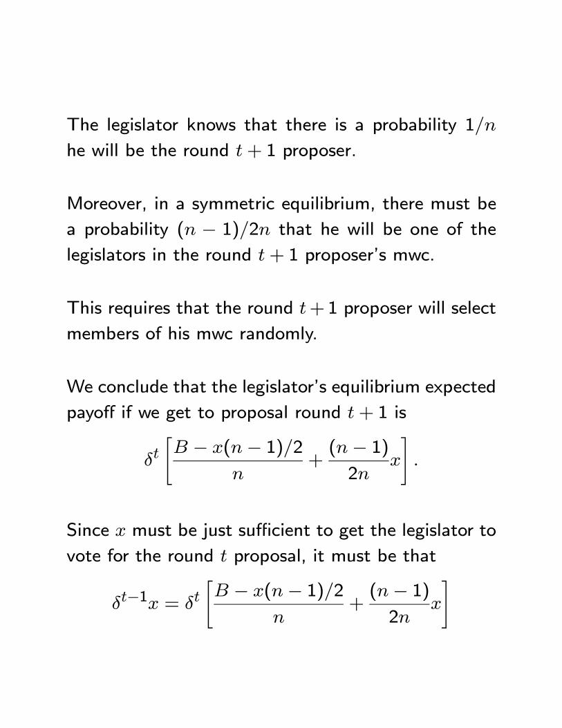
The legislator knows that there is a probability 1

he will be the round + 1 proposer.

Moreover, in a symmetric equilibrium, there must be

a probability ( − 1)2 that he will be one of the

legislators in the round + 1 proposer’s mwc.

This requires that the round +1 proposer will select

members of his mwc randomly.

We conclude that the legislator’s equilibrium expected

payoff if we get to proposal round + 1 is

" − (− 1)2

+(− 1)2

#

Since must be just sufficient to get the legislator to

vote for the round proposal, it must be that

−1 = " − (− 1)2

+(− 1)2

#

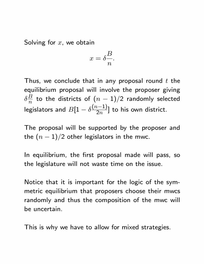
Solving for , we obtain

=

Thus, we conclude that in any proposal round the

equilibrium proposal will involve the proposer giving

to the districts of ( − 1)2 randomly selected

legislators and [1− (−1)2 ] to his own district.

The proposal will be supported by the proposer and

the (− 1)2 other legislators in the mwc.

In equilibrium, the first proposal made will pass, so

the legislature will not waste time on the issue.

Notice that it is important for the logic of the sym-

metric equilibrium that proposers choose their mwcs

randomly and thus the composition of the mwc will

be uncertain.

This is why we have to allow for mixed strategies.

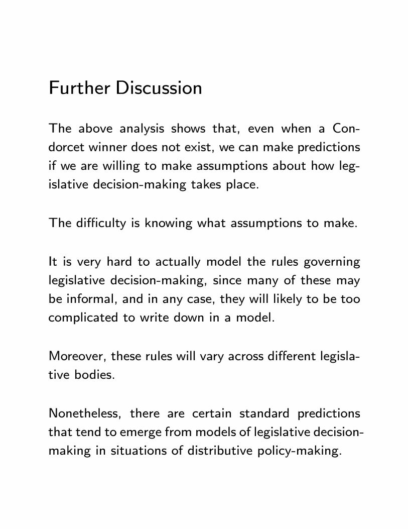
Further Discussion

The above analysis shows that, even when a Con-

dorcet winner does not exist, we can make predictions

if we are willing to make assumptions about how leg-

islative decision-making takes place.

The difficulty is knowing what assumptions to make.

It is very hard to actually model the rules governing

legislative decision-making, since many of these may

be informal, and in any case, they will likely to be too

complicated to write down in a model.

Moreover, these rules will vary across different legisla-

tive bodies.

Nonetheless, there are certain standard predictions

that tend to emerge from models of legislative decision-

making in situations of distributive policy-making.

First, the proposing legislator (or legislators if a com-

mittee is in charge of proposals) gets extra benefits

for his district.

Second, benefits are enjoyed by a mwc of legislators.

Third, which legislators are in the mwc is uncertain.

See Eraslan (2001) for a clean theoretical treatment

of the Baron-Ferejohn legislative bargaining model.

See Volden and Wiseman (2007) for a study of leg-

islative bargaining in which there are public goods as

well as transfers.

See Morelli (1999) for a slightly different approach to

modelling legislative bargaining.

See Frechette, Kagel, and Morelli (2005) for experi-

mental work on legislative bargaining.

See Knight (2005) for empirical evidence of ”proposal

power” in the allocation of Federal highway dollars.

Legislative Norms

An alternative (now less popular) approach to making

predictions in distributive policy settings is to assume

that legislators develop norms of behavior to overcome

the potential instability associated with the lack of a

Condorcet winner.

Weingast came up with the idea of a “norm of univer-

salism” (see Weingast, Shepsle, and Johnson (1981)

for discussion).

Suppose that the legislators are choosing the amount

to be spent on (say) transportation projects in each

legislator’s district.

Then a policy will be a vector (1 ) where is

the spending in legislator ’s district.

There is no predetermined budget, so the set of alter-

native policies is

= {(1 ) : ≥ 0 for all }

Assume that transportation spending is funded by a

uniform tax on all districts =P=1 .

Assume that

(1 ) = ()−

where (0) = 0 and (·) is increasing and strictlyconcave.

There is no Condorcet winner in this Example (Prove

yourself)

The norm of universalism works as follows: each leg-

islator chooses the amount of public spending that he

would like for his district.

These desired spending levels are then passed unani-

mously by the legislature.

The norm is “I will vote for your pet projects, with

the understanding that you will vote for mine” or “you

scratch my back and I will scratch yours”

Let (∗1 ∗) be the equilibrium spending levels.

Then,

∗ = argmax(∗1 ∗)

This implies that ∗ = ∗ where

0(∗) = 1

This leads to the Law of 1/n which says that, ceteris

paribus, the greater the number of legislative districts,

the greater the amount of public spending.

Interestingly, there is a considerable amount of evi-

dence for the Law of 1/n - see Baqir (2002) for evi-

dence from U.S. cities.

Equilibrium spending is too high when compared to

the surplus maximizing per district spending level which

is = where

0() = 1

The theory suggests that all districts will get spending,

which distinguishes it from the predictions of legisla-

tive bargaining models.

Despite seeming eminently sensible, the postulated

behavior of the legislators is hard to make sense of.

At the time of voting for the omnibus bill, all the

legislators would be better off agreeing to reduce all

their spending levels.

This observation has led the model to lose favor in

the theoretical literature.

I.4 Interest Groups

Interest groups are groups of citizens who share com-

mon policy objectives and seek to influence policy in

a coordinated way.

Important examples in American politics are the NRA,

the AARP, the AMA, the Sierra Club, the NAACP, the

ACLU, Common Cause, and the Humane Society.

We will discuss how and why interest groups are formed

and then how they influence policy determination.

We will consider two different avenues of influence:

lobbying and campaign contributions.

I.4.i Interest Group Formation

There are many different groups of citizens who share

common policy objectives.

For example, college students who share an interest

in lower tuition at state universities, university profes-

sors who share an interest in more government funding

for research, pet lovers who share an interest in gov-

ernment subsidization of no-kill animal shelters and

spaying and neutering programs, smokers who share

an interest in lower cigarette taxes, etc, etc.

What determines which groups will form an interest

group and seek to influence policy?

This is a difficult problem for the economic approach

to politics because interest group formation involves

the voluntary provision of what is essentially a public

good for potential group members.

The economic approach suggests that public goods

will not be voluntarily provided or, if they are, will be

provided at extremely low levels.

This is because of the well-known free rider problem.

To illustrate the problem, suppose that an interest

group entrepreneur decides to try and form an envi-

ronmental interest group.

Suppose that there are environmentally concerned

citizens and the entrepreneur asks each to contribute

to the interest group.

Let citizen ’s contribution be denoted and the total

contributions to the interest group be denoted =P .

Let the stringency of environmental regulation chosen

by the government be denoted by .

Assume that the environmental interest group will use

its contributions to try to get more stringent regula-

tions.

Thus, assume that = 0 + 1 where 0 and 1satisfy 1 0 ≥ 0

Let citizen ’s payoff be

ln −

Thus, citizen likes more stringent regulation, but

does not like contributing.

The per-citizen contribution that maximizes the ag-

gregate utility of the environmentally concerned cit-

izens is

= argmax [ln (0 + 1)− ]

This satisfies the first order condition

1

0 + 1= 1

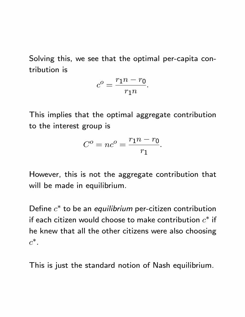
Solving this, we see that the optimal per-capita con-

tribution is

=1− 0

1

This implies that the optimal aggregate contribution

to the interest group is

= =1− 0

1

However, this is not the aggregate contribution that

will be made in equilibrium.

Define ∗ to be an equilibrium per-citizen contributionif each citizen would choose to make contribution ∗ ifhe knew that all the other citizens were also choosing

∗.

This is just the standard notion of Nash equilibrium.

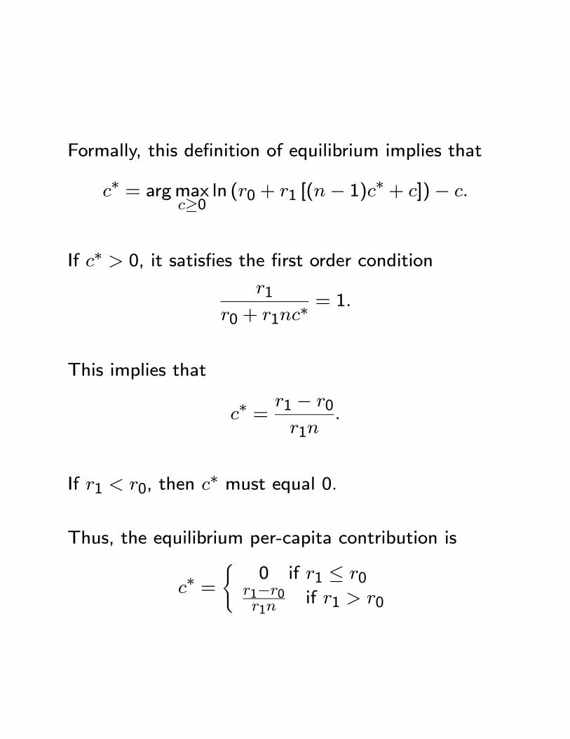
Formally, this definition of equilibrium implies that

∗ = argmax≥0

ln (0 + 1 [(− 1)∗ + ])−

If ∗ 0, it satisfies the first order condition

1

0 + 1∗ = 1

This implies that

∗ = 1 − 0

1

If 1 0, then ∗ must equal 0.

Thus, the equilibrium per-capita contribution is

∗ =(

0 if 1 ≤ 01−01

if 1 0

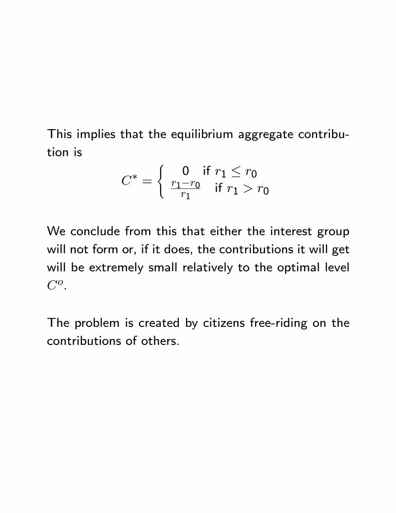
This implies that the equilibrium aggregate contribu-

tion is

∗ =(

0 if 1 ≤ 01−01

if 1 0

We conclude from this that either the interest group

will not form or, if it does, the contributions it will get

will be extremely small relatively to the optimal level

.

The problem is created by citizens free-riding on the

contributions of others.

Olson’s Ideas

So how can we explain the fact that interest groups

do form?

Mancur Olson suggested two explanations in a famous

book The Logic of Collective Action.

First, he argued that small groups who have large po-

tential benefits from influence activities will be better

able to overcome the free rider problem.

Thus, for example, industries which consist of rela-

tively few firms should be able to coordinate their ac-

tivities.

This contrasts with consumer interest groups, which

should be rather rare.

The theoretical case for this argument is not com-

pletely clear (see Esteban and Ray (2001)).

In our model, for example, while equilibrium per-capita

contributions are decreasing in , the aggregate con-

tribution is actually independent of .

More relevant for Olson’s argument may be the the-

ory of repeated games which shows that the free-rider

problem can be overcome in dynamic contexts.

The optimal outcome may be sustained by the threat

that if one player free-rides, the others will revert to

free-riding behavior in the future.

Coordinating on this good outcome may be easier in

small groups because it is easier for group members

to monitor the behavior of other group members.

Thus, in industries which consist of relatively few firms,

if one firm is not paying its fair contribution to the in-

dustry’s influence activities, the other firms should be

able to observe this and react accordingly.

Second, Olson argued that interest groups who can

supply their members private goods will be more likely

to be successful.

Possible private goods consist of buttons, decals, bumper

stickers, mugs, magazines, newsletters, discounts on

insurance, discounts on hotels, stuffed toys, etc.

To illustrate this idea, suppose that our interest group

entrepreneur in exchange for a contribution offers an

amount of interest group-related private goods .

Suppose that the cost to the entrepreneur of providing

a unit of one of these private goods is .

This means that if total contributions are , the rev-

enues the interest group has left over for influencing

policy are (1− )

Suppose that citizen ’s payoff is

ln + ln −

where denotes interest group-related private goods

and 0.

Then the equilibrium per-citizen contribution ∗ solvesthe problem

∗ = argmax≥0

ln {0 + 1 [((− 1)∗ + ) (1− )]}+ ln −

The first order condition is

1(1− )

0 + 1∗(1− )

+

∗= 1

In general this is a quadratic equation in ∗, but tomake it a linear equation lets assume that 0 = 0.

Then we have a very simple solution

∗ = 1

+

This implies that aggregate contributions are

∗ = 1 +

and profits are

(1 + ) (1− )

Observe that as long as the entrepreneur keeps

small, he can get significantly more contributions for

the interest group in this way.

Discussion

There seems to be some truth to Olson’s ideas.

Industry-based interest groups do seem common (to-

bacco companies, automobile manufacturers, boat man-

ufacturers, beverage producers, etc, etc).

Citizen-based groups do indeed offer members private

goods in exchange for contributions.

The AARP offers a magazine and numerous discounts,

the NRA provides a magazine and accidental death

insurance, the World Wildlife Fund offers stuffed tigers

and opportunities to adopt animals.

However, Olson’s private good theory does not explain

why these private goods cannot be provided by entre-

preneurs who do not have the additional cost burden

associated with influence activities.

Nor does his private good theory give us a particularly

sharp answer to our question of which interest groups

will form.

Moreover, in general, Olson’s concern with free-riding

is a bit too pessimistic regarding human nature.

Free-riding has been subject to intense scrutiny in lab-

oratory experiments and people contribute much more

than theory predicts.

On the basis of this evidence, we would expect a sig-

nificant fraction of people to contribute to interest

groups who champion issues they care about.

Why people do this is not really clear - they may be

choosing to behave as rule utilitarians as we discussed

earlier in the context of voting.

The bottom line is that the literature has not really

produced a compelling answer to the question of in-

terest group formation.

From now on, we will assume that interest groups

exist and analyze how they influence policy outcomes.

I.4.ii Interest Group Influence by Lob-bying

Interest groups in the U.S. spend a considerable amount

lobbying Congress and Federal Agencies.

They do this either by hiring the services of a lobbying

firm or by employing their own “in house” lobbyist.

OpenSecrets.org reports that in 2008 the total amount

spent on lobbying the U.S. federal government was

$3.3bn and there were 14,800 registered lobbyists.

Presumably, interest groups would not spend all this

money on lobbying unless it was effective.

A large literature explores why and how lobbying works.

Informational Lobbying

One strand of literature views lobbying as providing

information to legislators concerning the impact of

proposed policy changes on their constituents.

In many circumstances interest groups will have much

more information on how a proposed policy will impact

their members than do politicians.

Providing such information can change legislators’ de-

cisions.

For example, suppose that a legislator is thinking of

voting for eliminating a tariff on a particular manu-

factured good and one consideration is how this will

impact the domestic industry in his district.

Suppose that he would favor elimination if the harm

to the domestic industry is low and be against if it

was high.

Suppose that he does not know for sure whether the

harm is low or high, but given his prior beliefs, is in-

clined to favor tariff elimination.

Then, the industry’s interest group can change the

legislator’s preferences by convincing him that the harm

is actually likely to be high.

Of course, the legislator should rationally be a bit

sceptical of the interest group’s claims.

An important concept in the theoretical literature is

therefore the provability of information.

The literature distinguishes full provability, partial prov-

ability, and no provability.

With full provability, an interest group can prove the

validity of its information - for example, present a sta-

tistical study of the effect of removing the tariff.

With no provability, it is unable to do this.

With partial provability it can present partial proof.

With full provability the issue is whether an interest

group will choose to reveal its information; that is,

which facts will it keep to itself and which facts will

it convey to policy-makers.

With no provability, the issue is how an interest group

credibly convey its information.

The majority of the theoretical literature focuses on

the case of no provability, so called “cheap talk”.

The literature shows that even in this case, and inter-

est group can influence policy as long as its preferences

are not too far apart from the policy-maker’s.

The Cheap Talk Model

There is a single policy maker and a single interest

group.

The policy maker has to choose the level of some

policy ∈ <

The optimal level of the policy depends upon the the

state of nature ∈ [min max]

The state of nature is the realization of a random

variable with CDF () and density ().

Assume that () 0 for all ∈ [min max]

The state of nature is observed by the interest group

but not the policy maker.

The policy maker’s preferences are

( ) = −(− )2

The interest group’s preferences are

( ) = −(− − )2

where 0.

Thus, the interest group prefers a larger level of the

policy than the policy-maker and measures the de-

gree of non-alignment.

Game and Equilibrium

The interest group observes the state of nature

The interest group then sends some message ∈

to the policy-maker - is the message space

The policy-maker observes the message and chooses

some policy

A strategy for the interest group is a function :

[min max]→ .

A strategy for the policy-maker is a function : →<

The policy-maker also has beliefs which are repre-

sented by the conditional CDF ( |) with density( |).

Thus,(0 |) is the probability that the policy-makerassigns to the state being less than 0 given that hehears the message

An equilibrium is {; ;} such that is optimal forthe interest group given ; is optimal for the policy-

maker given his beliefs ; and is consistent with

where possible.

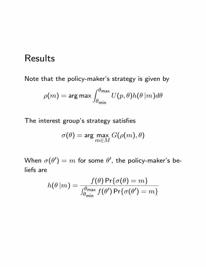
Results

Note that the policy-maker’s strategy is given by

() = argmax

Z max

min( )( |)

The interest group’s strategy satisfies

() = arg max∈

(() )

When (0) = for some 0, the policy-maker’s be-liefs are

( |) = () Pr{() = }R maxmin

(0) Pr{(0) = }

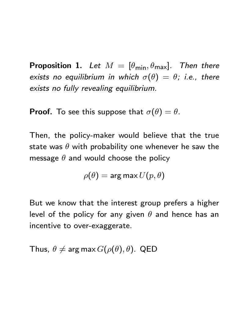
Proposition 1. Let = [min max]. Then there

exists no equilibrium in which () = ; i.e., there

exists no fully revealing equilibrium.

Proof. To see this suppose that () = .

Then, the policy-maker would believe that the true

state was with probability one whenever he saw the

message and would choose the policy

() = argmax( )

But we know that the interest group prefers a higher

level of the policy for any given and hence has an

incentive to over-exaggerate.

Thus, 6= argmax(() ). QED

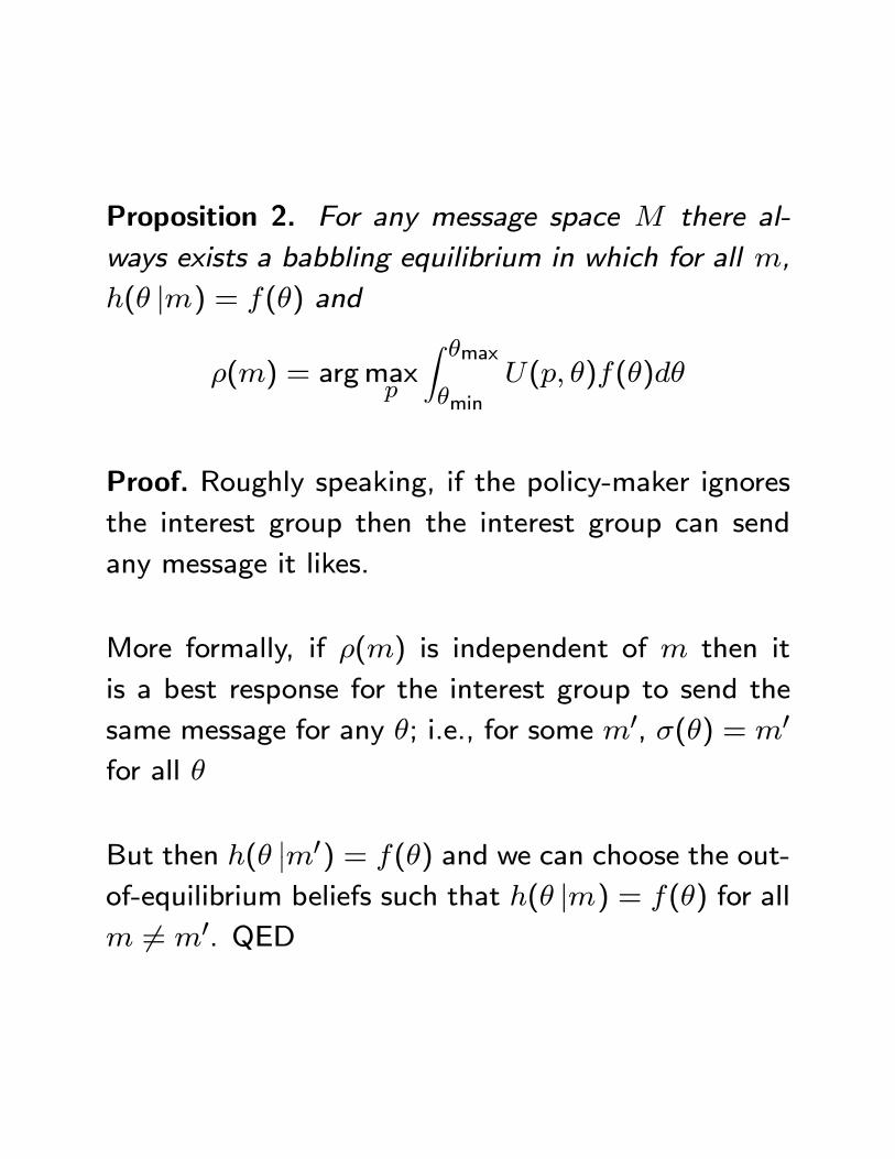
Proposition 2. For any message space there al-

ways exists a babbling equilibrium in which for all ,

( |) = () and

() = argmax

Z max

min( )()

Proof. Roughly speaking, if the policy-maker ignores

the interest group then the interest group can send

any message it likes.

More formally, if () is independent of then it

is a best response for the interest group to send the

same message for any ; i.e., for some 0, () = 0

for all

But then (¯̄0) = () and we can choose the out-

of-equilibrium beliefs such that ( |) = () for all

6= 0. QED

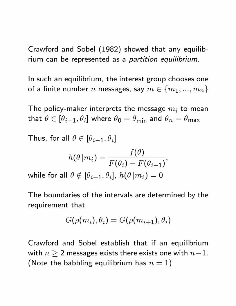
Crawford and Sobel (1982) showed that any equilib-

rium can be represented as a partition equilibrium.

In such an equilibrium, the interest group chooses one

of a finite number messages, say ∈ {1 }

The policy-maker interprets the message to mean

that ∈ [−1 ] where 0 = min and = max

Thus, for all ∈ [−1 ]

( |) =()

()− (−1)

while for all ∈ [−1 ], ( |) = 0

The boundaries of the intervals are determined by the

requirement that

(() ) = ((+1) )

Crawford and Sobel establish that if an equilibrium

with ≥ 2 messages exists there exists one with −1.(Note the babbling equilibrium has = 1)

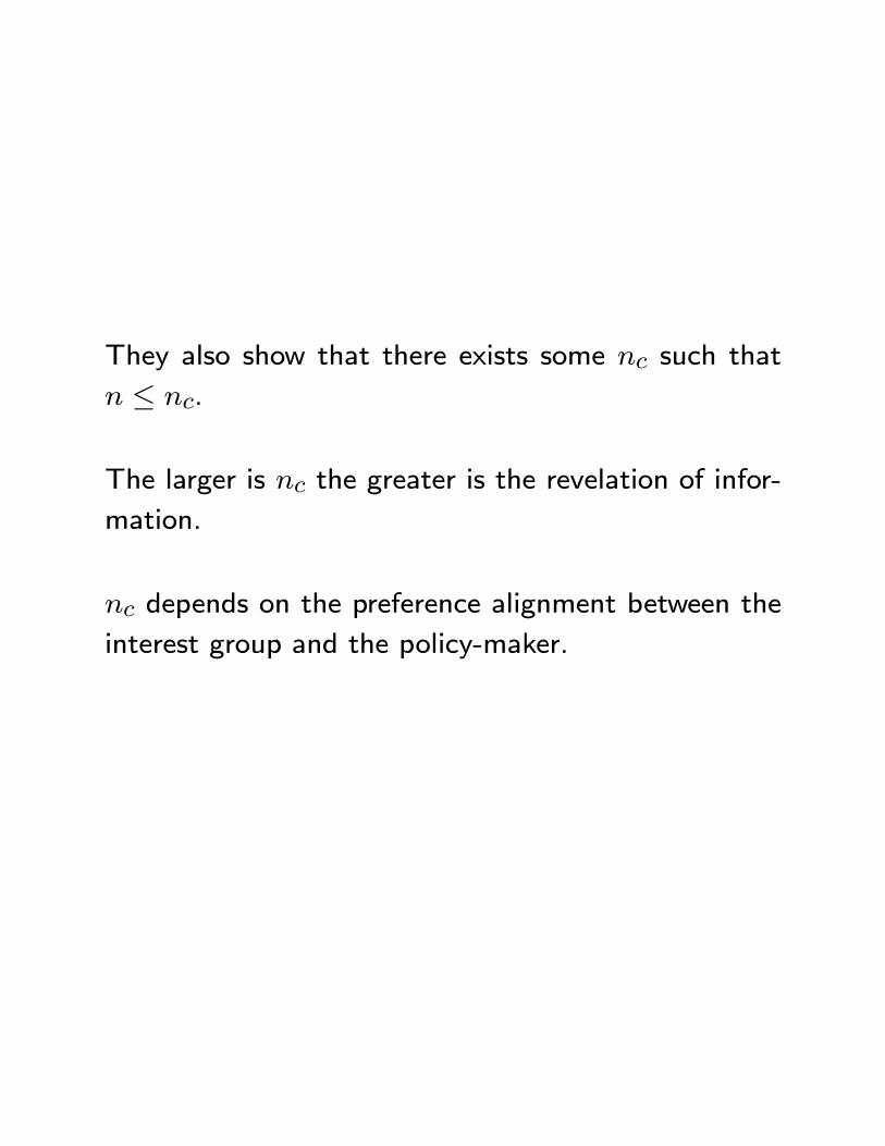
They also show that there exists some such that

≤ .

The larger is the greater is the revelation of infor-

mation.

depends on the preference alignment between the

interest group and the policy-maker.

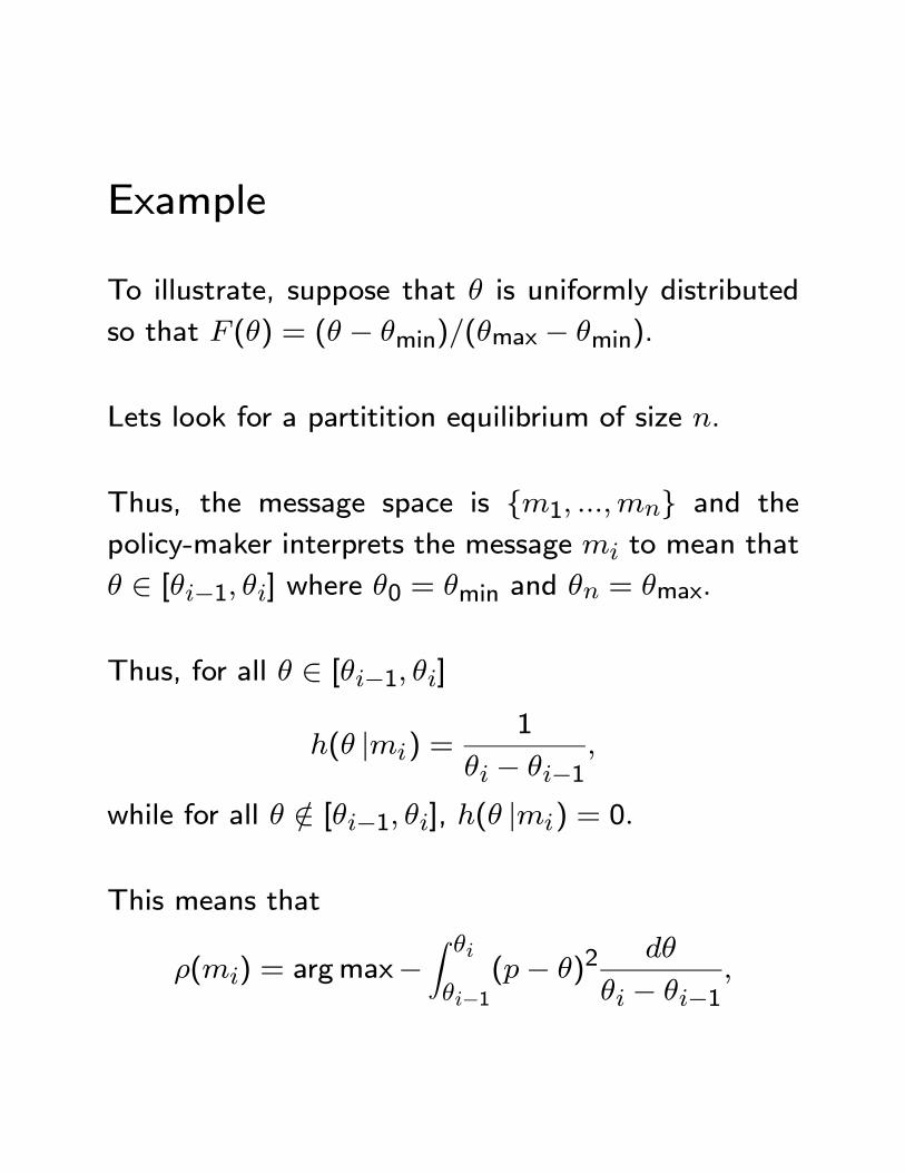
Example

To illustrate, suppose that is uniformly distributed

so that () = ( − min)(max − min).

Lets look for a partitition equilibrium of size .

Thus, the message space is {1 } and thepolicy-maker interprets the message to mean that

∈ [−1 ] where 0 = min and = max.

Thus, for all ∈ [−1 ]

( |) =1

− −1

while for all ∈ [−1 ], ( |) = 0

This means that

() = argmax−Z

−1(− )2

− −1

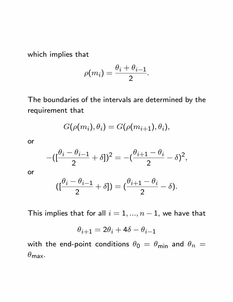
which implies that

() = + −1

2

The boundaries of the intervals are determined by the

requirement that

(() ) = ((+1) )

or

−([ − −12

+ ])2 = −(+1 −

2− )2

or

([ − −1

2+ ]) = (

+1 −

2− )

This implies that for all = 1 − 1, we have that

+1 = 2 + 4 − −1with the end-point conditions 0 = min and =

max.

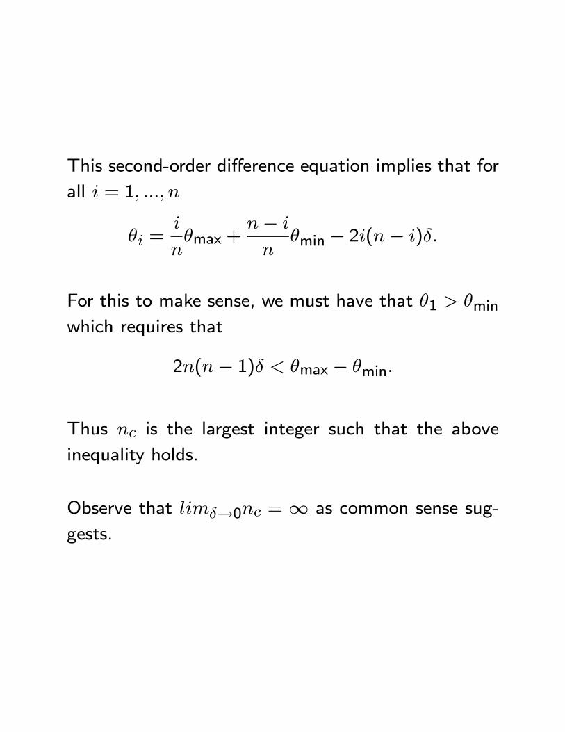
This second-order difference equation implies that for

all = 1

=

max +

−

min − 2(− )

For this to make sense, we must have that 1 min

which requires that

2(− 1) max − min

Thus is the largest integer such that the above

inequality holds.

Observe that →0 = ∞ as common sense sug-

gests.

This type of model can be extended to include two

interest groups - see Krishna and Morgan (2001)

It can also be extended to have a multidimensional

policy space - see Battaglini (2003)

One can also extend the model to have costly infor-

mation acquisition and so on.

Lobbying as Legislative Subsidy

A recent paper by Hall and Deardoff (2006) offers a

slightly different take on what lobbying does.

They develop a theory based on the following five as-

sumptions.

Assumption 1: For a legislator to have much influence

on policy, he must work at it.

Assumption 2: Legislators’ resources are scarce.

Assumption 3: At any given point in time, individ-

ual legislators care about influencing more than one

policy.

Assumption 4: Legislators care about some issues

more than others.

Assumption 5: Relative to legislators, lobbyists are

specialists.

Given these assumptions, the main elements of Hall

and Deardoff’s theory can be represented as a simple

consumer choice problem.

The legislator cares about “making progress” on some

target issue and on an aggregate of other issues .

By making progress, is meant moving policy closer to

their preferred level by introducing a bill, making an

amendment to an existing bill, influencing a govern-

ment agency, fighting against a bad bill, etc.

Letting denote progress on issue and progress

on other issues, we can write the legislator’s utility

function as ( ).

The legislator must chooses how much effort to devote

to issue and the other issues.

Let denote effort devoted to issue and denote

effort devoted to other issues.

The constraint that the legislator’s resources are scarce

can be modeled by assuming that

+ ≤ max

Assuming that = and = for some

0, the legislator’s problem in the absence of lobbying

can be posed as

max( )

+ ≤ max

This is a standard consumer choice problem which

can be represented diagrammatically with the usual

indifference curve and budget line diagram.

Without lobbying there will be some optimal choice

( ∗ ∗ ).

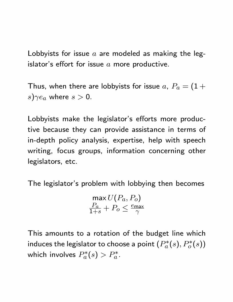
Lobbyists for issue are modeled as making the leg-

islator’s effort for issue more productive.

Thus, when there are lobbyists for issue , = (1+

) where 0.

Lobbyists make the legislator’s efforts more produc-

tive because they can provide assistance in terms of

in-depth policy analysis, expertise, help with speech

writing, focus groups, information concerning other

legislators, etc.

The legislator’s problem with lobbying then becomes

max( )1+

+ ≤ max

This amounts to a rotation of the budget line which

induces the legislator to choose a point ( ∗ () ∗ ())which involves ∗ () ∗ .

In this way, lobbying leads to greater progress being

made on issue .

The problem with this analysis is that it does not

recognize that collective action by legislators is neces-

sary to make progress on an issue.

Thus just focusing on a single legislator is not fully

satisfying, since no such legislator can make progress

alone.

It may be possible to extend the theory to capture

this.

Evidence

The above two stories explain theoretically why lob-

bying legislators may produce results.

There have been few successful empirical attempts to

measure the returns to lobbying.

One interesting effort is by de Figueiredo and Silver-

man (2006) who look at university lobbying.

They measure the outcome variable as the amount of

educational spending earmarked to go to fund projects

at a university.

The vast majority of federal money financing academic

research is allocated by federal agencies (such as the

NSF and NIH) using competitive peer reviews.

However, a significant chunk (around 10% at the time

de Figueiredo and Silverman wrote their article) is al-

located via earmark.

de Figueiredo and Silverman ran regressions with ear-

marked spending to University x as the dependent

variable and the amount spent on lobbying by Uni-

versity x as the independent variable.

They find no returns to lobbying for universities whose

Congressman or Senator is not on either the Senate

or House Appropriations Committtees.

However, the average university whose senator is on

the Senate Appropriations Committee receives an av-

erage return on $1 of lobbying spending in the range

of $11-$17.

The average university whose congressman is on the

House Appropriations Committee receives an average

return on $1 of lobbying spending in the range of $20-

$36.

These are very significant returns!

I.5.iii Interest Group Influence byCam-paign Contributions

A campaign contribution is an amount of money given

to a politician to help him finance his campaign to get

elected.

Such contributions are used by politicians to finance

campaign advertisements, town hall meetings, voter

turnout efforts, etc.

According to OpenSecrets.org, the total amount spent

in the 2008 election cycle in House, Senate and Pres-

idential races was $3.1bn.

Contributions are made by individual citizens and Po-

litical Action Committees (PACs).

When an interest group, union, or corporation wants

to contribute to federal candidates or parties, it must

do so through a PAC.

Examples of PACs are the Sierra Club Political Com-

mittee, the League of Conservation Voters Action Fund,

the National Rifle Association Political Victory Fund,

the National Association of Realtors PAC, the Planned

Parenthood Action Fund, the American Beverage As-

sociation PAC, the American Beer Companies PAC,

and the American Automobile Manufacturers PAC.

Corporations and unions may not contribute directly

to federal PACs, but they may pay for the administra-

tive costs of an affiliated PAC.

Corporate-affiliated PACs may only solicit contribu-

tions from executives, shareholders, and their families,

while union-affiliated PACs may only solicit contribu-

tions from members.

Overall, PACs account for less than thirty percent of

total contributions in U.S. Congressional races, and

considerably less in presidential races.

The amount that individuals and PACs can give to

any one candidate is limited.

The individual limit per candidate is $2400 per elec-

tion and the PAC limit per candidate is $5000 per

election.

For more information go to the website of the Federal

Election Commission (FEC).

All the individual U.S. states have their own regula-

tions concerning state elections.

A large academic literature addresses how campaign

contributions by interest groups impact policy out-

comes.

The topic is a complex one since a good theory should

(i) explain how and why campaign spending impacts

voter behavior, and (ii) why contributors give to can-

didates.

These are issues on which common sense and the em-

pirical literature offer no clear guidance.

Campaign Spending and Voter Be-havior

In the theoretical literature, there are two main ways

to think about how and why campaign spending im-

pacts votes.

First, spending buys the votes of “noise voters”.

Noise voters are analogous to noise traders in financial

markets.

These are voters who are voting for random non-policy

related reasons.

Campaign advertising is simply assumed to attract

these voters.

Second, spending allows candidates to provide infor-

mation about their accomplishments and policy posi-

tions to uninformed voters.

In this view, voters are rational and update their be-

liefs based on the information they see in campaign

advertising.

Gerber, Gimbel, Green, and Shaw (2011) run an in-

teresting field experiment where they try to assess the

impact of campiagn advertising on voters’ preferences.

They worked with the Rick Perry campaign in the

2006 Texas Gubernatorial Race.

Perry, the incumbent, was running for re-election and

the experiment took place during the early months

of the campaign (Jan 2006), before the full field of

candidates had become clear.

The experiment randomized the deployment of an ad-

vertisment which listed some of the accomplishments

of Texas during Perry’s first term.

Using surveys of treated voters, they found that the

advertising campaign caused a large initial boost in

support for Perry, but this effect diminished rapidly

over time.

They argue that this up and then down pattern is not

consistent with opinion change due to informational

updating.

Independent of why campaign spending impacts voter

behavior, there is the question of the magnitude of the

effects.

In fact, there is a good deal of debate empirically on

the impact of campaign spending on votes (see Gerber

(2004) for a review).

Estimating a causal effect is a difficult econometric

problem because of the endogeneity of campaign spend-

ing.

For example, a good candidate will presumably attract

more contributions leading to a positive correlation

between votes and money.

On the other hand, an incumbent who is facing a high

quality challenger will presumably seek more contribu-

tions and spend more, than an incumbent facing a low

quality challenger, leading to a negative correlation

between votes and money.

The general conclusions are that campaign spending

by incumbents in the U.S. House does not have a

significant effect on their vote share, whereas spending

by challengers does.

By contrast, spending by both incumbents and chal-

lengers in U.S. Senate races has a significant effect,

although spending by challenegers is more effective.

It is not clear how sensible the result concerning House

incumbents is, given how much time incumbents de-

vote to raising contributions.

Why do Interest Groups Give?

On the question of why contributors give, the central

issue is whether contributions are used to influence

politicians, or whether contributors just give to help

get their preferred politicians elected.

Influence can take the form of buying votes or buying

access.

Access means the opportunity to present persuasive

information.

The idea is that if a politician has received a con-

tribution from someone, a politician is more likely to

agree to listen to a contributor’s argument concerning

a proposed piece of legislation.

Economic approaches to politics tend to focus on the

influence motive for giving as opposed to the electoral

motive.

This is because giving to help get a preferred candi-

date elected is like making a voluntary contribution to

a public good for the supporters of this candidate.

As we have already seen, the economic approach sug-

gests that public goods will not be voluntarily provided

or, if they are, will be provided at extremely low levels.

However, as we have seen, people do contribute more

to public goods than the economic approach would

suggest.

Ansolabehere, de Figueiredo, and Snyder (2003) make

a strong case against the practical importance of the

influence motive in U.S. national politics.

They argue that if politicians could be so influenced,

then given the size of federal government spending,

there would be way more money in U.S. politics than

there is.

On the other hand, Jayachandran (2006) documents

significant negative effects on the stock market val-

ues of firms contributing soft money to the Repub-

lican party from Senator Jeffords 2001 switch from

the Republican party which tipped the balance of the

Senate.

“Soft money” refers to unregulated contributions to

national parties that were since banned by the McCain-

Feingold Act of 2002.

One interpretation of her finding is that the stock mar-

ket anticipated that these firms would now have less

influence over policy because the party they supported

no longer controlled the agenda.

Also Mian, Sufi, and Trebbi (2009) document an as-

sociation between higher campaign contributions from

the financial services industry and voting in favor of

a bill which transfered money from taxpayers to the

industry (The Emergency Economic Stabilization Act

of 2008).

The suggestion is that these contributions bought votes.

While suggestive, neither of these papers conclusively

establish an influence motive.

It could be that the contributions were simply given

because of the policy preferences of the party or leg-

islators.

There is quite a bit of anecdotal evidence from Con-

gressmen and Senators in favor of the idea that con-

tributions do buy access.

That is, these politicians report that they do feel oblig-

ated to meet with those citizens who have supported

them with significant contributions.

Presumably, if an interest group receives better access

this should translate into obtaining better policy out-

comes, but this part of the link is not well-established

empirically.

The Common Agency Model

The simplest economic model of interest group influ-

ence by campaign contributions is the common agency

model.

The model assumes that there are interest groups

competing to influence a politician who must choose

some policy ∈ .

The idea is that the politician is already in office and

having to make policy decisions, but needs campaign

contributions to run for re-election in the future.

If the politician receives an aggregate contribution

from the interest groups and chooses policy he re-

ceives a payoff 0() + .

The idea is that the politician cares about the policy

decision he makes but also values contributions for his

re-election campaign.

The latter is modeled in a reduced form way by just

assuming that the politician’s payoff depends on his

aggregate contributions.

If interest group makes a contribution and the

politician chooses policy , its payoff is ()− .

Thus, interest groups do not like making contribu-

tions.

Game and Equilibrium

The interaction between the interest groups and the

politician is modelled as a two-stage game.

In Stage 1 each interest group independently and si-

multaneously offers the politician a contribution sched-

ule () which describes the contribution it will make

conditional on the policy choice that he makes.

In Stage 2 the politician chooses policy taking into

account the implications of his choice for the contri-

butions he will receive.

Given the interest groups’ contribution schedules

1(·) (·), the politician will choose a policyfrom the set

(1(·) (·)) = argmax∈

[0() +X=1

()]

Thus, the politician will trade off his own policy pref-

erences with the impact of his policy choice on the

contributions that he will receive.

The contribution schedules ∗1(·) ∗(·) and thepolicy choice ∗ represent an equilibrium if (i)

∗ ∈(∗1(·) ∗(·))and (ii) there is no interest group , contribution sched-

ule (·) and policy choice ∈(∗1(·) (·) ∗(·))such that

()− () (∗)− ∗ (∗)

Thus, in equilibrium we require (i) that the politician

be choosing an optimal policy given the contribution

schedules he faces, and (ii) that no interest group can

alter its contribution schedule to achieve a preferred

outcome.

Results

Consider first the case of a single interest group.

If there were no contributions, the politician would

simply choose his preferred policy

0 = argmax∈

0()

The interest group can get the politician to choose any

policy as long as it provides him with a contribution

1 such that

0() + 1 ≥ 0(0)

The interest group’s problem can therefore be posed

as:

max(1) 1()− 1 0() + 1 ≥ 0(0)

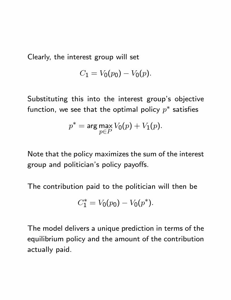
Clearly, the interest group will set

1 = 0(0)− 0().

Substituting this into the interest group’s objective

function, we see that the optimal policy ∗ satisfies

∗ = argmax∈

0() + 1()

Note that the policy maximizes the sum of the interest

group and politician’s policy payoffs.

The contribution paid to the politician will then be

∗1 = 0(0)− 0(∗)

The model delivers a unique prediction in terms of the

equilibrium policy and the amount of the contribution

actually paid.

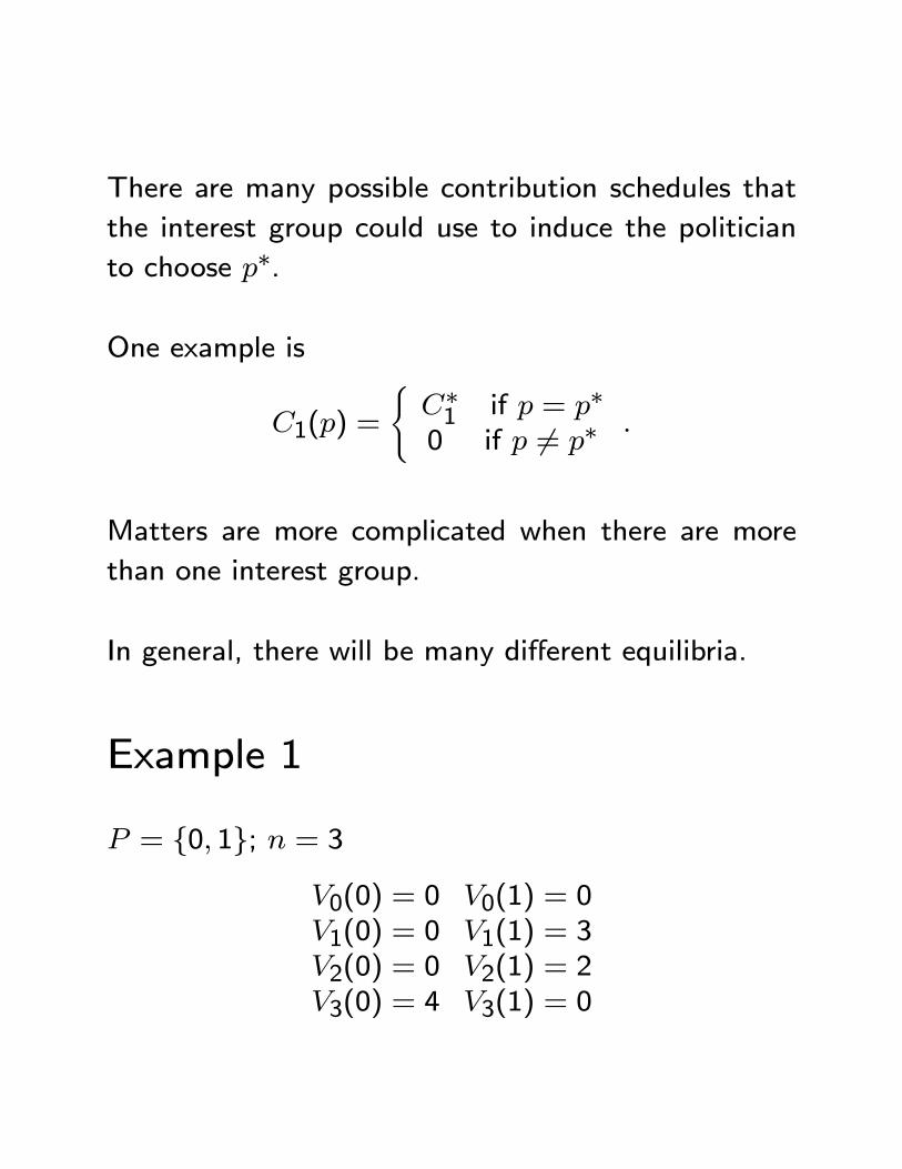
There are many possible contribution schedules that

the interest group could use to induce the politician

to choose ∗.

One example is

1() =

(∗1 if = ∗0 if 6= ∗

Matters are more complicated when there are more

than one interest group.

In general, there will be many different equilibria.

Example 1

= {0 1}; = 30(0) = 0 0(1) = 0

1(0) = 0 1(1) = 3

2(0) = 0 2(1) = 2

3(0) = 4 3(1) = 0

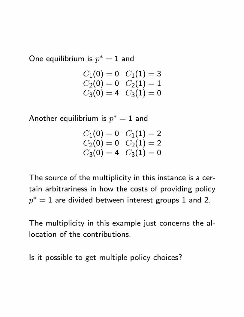
One equilibrium is ∗ = 1 and

1(0) = 0 1(1) = 3

2(0) = 0 2(1) = 1

3(0) = 4 3(1) = 0

Another equilibrium is ∗ = 1 and

1(0) = 0 1(1) = 2

2(0) = 0 2(1) = 2

3(0) = 4 3(1) = 0

The source of the multiplicity in this instance is a cer-

tain arbitrariness in how the costs of providing policy

∗ = 1 are divided between interest groups 1 and 2.

The multiplicity in this example just concerns the al-

location of the contributions.

Is it possible to get multiple policy choices?

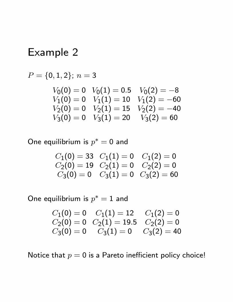
Example 2

= {0 1 2}; = 30(0) = 0 0(1) = 05 0(2) = −81(0) = 0 1(1) = 10 1(2) = −602(0) = 0 2(1) = 15 2(2) = −403(0) = 0 3(1) = 20 3(2) = 60

One equilibrium is ∗ = 0 and

1(0) = 33 1(1) = 0 1(2) = 0

2(0) = 19 2(1) = 0 2(2) = 0

3(0) = 0 3(1) = 0 3(2) = 60

One equilibrium is ∗ = 1 and

1(0) = 0 1(1) = 12 1(2) = 0

2(0) = 0 2(1) = 195 2(2) = 0

3(0) = 0 3(1) = 0 3(2) = 40

Notice that = 0 is a Pareto inefficient policy choice!

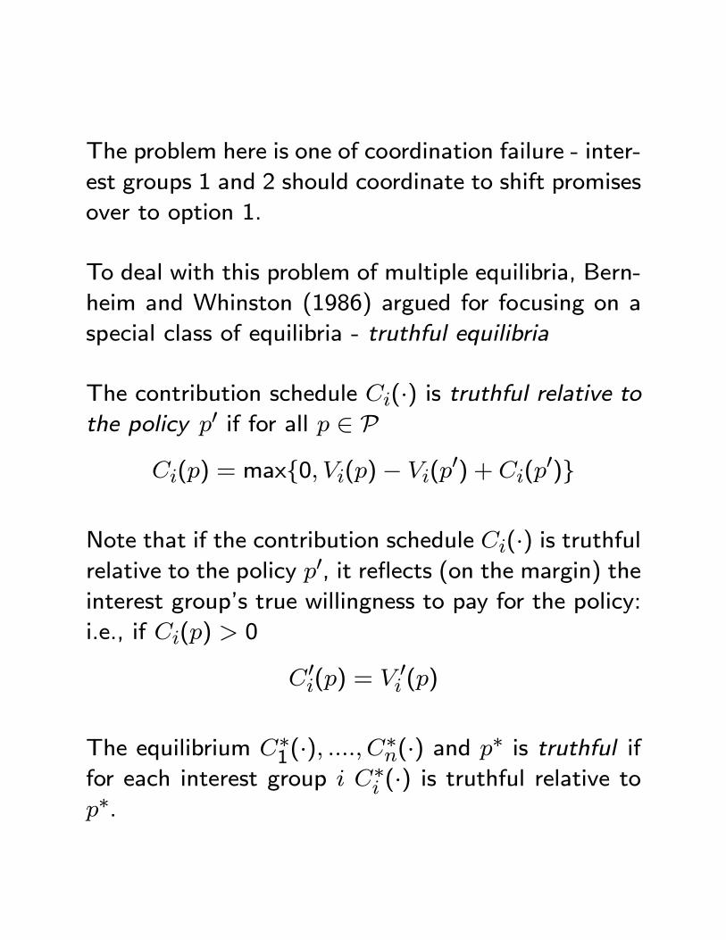
The problem here is one of coordination failure - inter-

est groups 1 and 2 should coordinate to shift promises

over to option 1.

To deal with this problem of multiple equilibria, Bern-

heim and Whinston (1986) argued for focusing on a

special class of equilibria - truthful equilibria

The contribution schedule (·) is truthful relative tothe policy 0 if for all ∈ P

() = max{0 ()− (0) + (

0)}

Note that if the contribution schedule (·) is truthfulrelative to the policy 0, it reflects (on the margin) theinterest group’s true willingness to pay for the policy:

i.e., if () 0

0() = 0 ()

The equilibrium ∗1(·) ∗(·) and ∗ is truthful iffor each interest group ∗ (·) is truthful relative to∗.

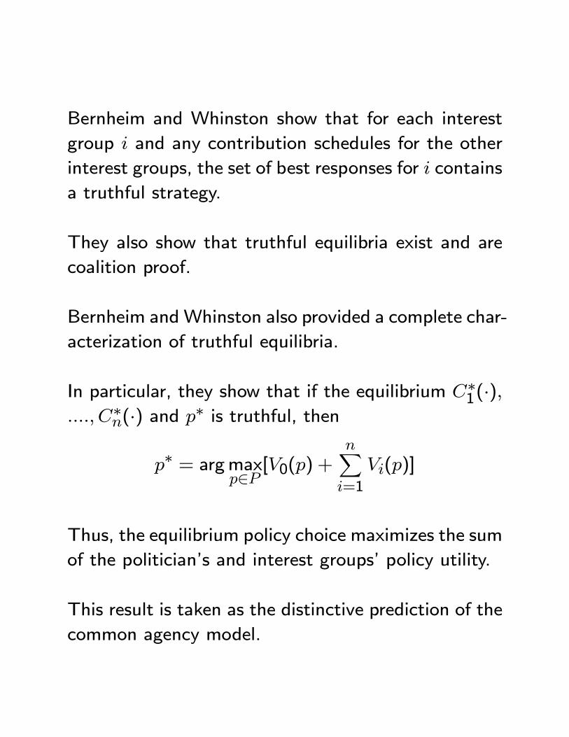
Bernheim and Whinston show that for each interest

group and any contribution schedules for the other

interest groups, the set of best responses for contains

a truthful strategy.

They also show that truthful equilibria exist and are

coalition proof.

Bernheim andWhinston also provided a complete char-

acterization of truthful equilibria.

In particular, they show that if the equilibrium ∗1(·) ∗(·) and ∗ is truthful, then

∗ = argmax∈

[0() +X=1

()]

Thus, the equilibrium policy choice maximizes the sum

of the politician’s and interest groups’ policy utility.

This result is taken as the distinctive prediction of the

common agency model.

It provides a concrete way of thinking about how cam-

paign contributions bias policy choices in favor of in-

terest groups.

Unfortunately, there is still multiplicity with respect

to contributions and in most applications the equilib-

rium contributions made by interest groups will not

typically be uniquely defined.

Bernheim and Whinston’s paper provides a complete

characterization of the contributions that are possible

in a truthful equilibrium.

Alternative Perspectives

The common agency model takes a very cynical view

of the influence of campaign contributions.

Contributions are essentially bribes paid by interest

groups in exchange for policy choices.

There is not much evidence to justify such a cynical

view.

The model also makes very strong assumptions about

the ability of interest groups to commit to deliver cam-

paign contribution promises.

That is, once the politician has chosen , what is to

stop the interest groups reneging on their promise to

contribute ()?

Fox and Rothenberg (2009) present an interesting po-

litical agency model showing how an interest group

can have significant influence on policy outcomes with-

out bribery or even spending any money at all.

This influence arises from the credible threat to con-

tribute to an incumbent’s challenger if the incumbent

votes against their position.

For example, suppose that you are a congressman who

has to decide whether to vote for a gun-control bill.

You know that if you vote in favor, the NRA will realize

that you are anti-gun and support your opponent in

the next primary or general election.

As a consequence, you abstain or vote against and

the gun-control bill fails without the NRA spending a

dime.

I.5 Political Parties

Political parties are groups of like-minded citizens who

collectively organize to elect candidates.

Party members provide support to their candidates in

the form of money and time.

Through their nominations, parties also provide can-

didates with a brand name which provides useful in-

formation to voters about candidates’ ideologies (see

Snyder and Ting (2002)).

In the legislature, political parties can pressure their

candidates to further the ideological goals of the party.

In this section, we briefly consider how parties im-

pact candidate competition and legislative decision-

making.

We take as given party membership, which seems a

reasonable short run assumption.

For models with endogenous party membership, see

Jackson and Moselle (2002), Levy (2004) and Roe-

mer.

I.5.i Parties and Candidate Competi-tion

In the U.S., political parties select candidates through

primary elections.

This is distinct from a system in which candidates are

selected by party elites.

The type of primary elections vary by state.

In closed primaries only party members are allowed to

vote, in open primaries voters can choose in which

primary to vote on the day of the election.

States are approximately evenly divided between open

and closed primaries (Gerber and Morton (1998)).

Primaries perform the function of winnowing the field

of candidates down to two, one from each party.

Independent or third party candidates are not common

in the U.S. and are rarely successful when they do run.

Primary elections can be straightforwardly incorpo-

rated into our earlier models of campaign competi-

tion.

We just need to categorize voters according to whether

they are registered Democrats, registered Republicans,

or unaffiliated.

Thus, we assume as before that citizens have ideolo-

gies distributed over the interval [0 1] and we let ()

be the fraction of voters with ideology ≤ .

But now we classify each voter as either a registered

Democrat, a registered Republican, or unaffiliated.

Let be the fraction of voters who are registered

Democrats and be the fraction of voters who are

registered Republicans.

Let () be the fraction of Democrats with ideology

≤ and () be the fraction of Republicans with

ideology ≤ .

It is natural to assume that Democrats are to the left

of the median voter and Republicans to the right.

We can identify a Democrat median voter and a

Republican median voter in the obvious way (i.e.,

and satisfy () = 12 and () =

12).

It will be the case that , where

is the aggregate median voter.

We also need to make an assumption as to how voters

in primary elections vote.

In particular, in primary elections the distinction be-

tween simple and sophisticated sincere voting is im-

portant.

With simple sincere voting, voters in the primary just

vote for the candidate who they like the best.

With sophisticated sincere voting, voters take into ac-

count how well candidates are going to perform in the

general election.

This may involve voting for a less preferred candidate

because he has a better chance in the general election.

For example, even if you really liked Dennis Kucinich,

you might have avoided voting for him in the 2008

Democratic primaries on the grounds that there was

no chance he could win the general election.

Downsian Candidates and Primaries

With simple sincere voting, the Downsian model pre-

dicts that candidates in closed primary elections would

adopt the ideology of the median party member and

then the ideology of the median voter in the general

election.

This is indeed quite consistent with the conventional

wisdom concerning candidate behavior in primaries

and general elections.

Candidates are often said to be moving to the center

after primary victories.

Nonetheless, the idea that candidates can completely

change their positions once they win the primary is

not very plausible.

With sophisticated sincere voting, whatever candidates

said about their ideologies during the primary elections

would be irrelevant as primary voters would anticipate

that the candidates would move to the center once

elected.

Thus, the Downsian perspective does not lend much

insight in this case.

Policy-motivated Candidates and Pri-maries

The most natural way to incorporate primaries into

the model of policy-motivated candidates is to assume

that primaries determine the true ideologies of the two

candidates competing in the general election.

Recall that in the model presented in I.2.ii, these true

ideologies were denoted and .

Thus, we can think of primary voters choosing be-

tween candidates on the basis of their true ideologies.

The winning candidates will then moderate their true

ideologies in the general election as in the model of

I.2.ii.

In this case, whether we assume primary voters vote

sincerely in a simple or sophisticated way will not mat-

ter.

With either form of voting, primary voters will want

to vote for candidates who share their true ideologies.

In a two-candidate closed primary race, therefore, the

candidate whose true ideology is closest to that of the

party median voter will win.

This provides some motivation for assuming that the

true ideologies and in the model of I.2.ii reflect

those of the party median voters; i.e., = and

= .

Under this assumption, for any given specification of

voters’ party affiliations, we obtain a complete model

of electoral competition which incorporates both pri-

mary and general elections.

Citizen-Candidates and Primaries

In a citizen-candidate model with closed primaries,

party members would select a candidate from those

citizens who have chosen to run in their party’s pri-

mary election.

In the general election, all voters would vote between

the candidates chosen in the two primaries.

Primaries would actually simplify the model because

they would ensure that the general election would only

involve two candidates (assuming the costs of running

as an independent candidate are prohibitive).

Whether primary voters vote sincerely in a simple or

sophisticated way will matter in the citizen-candidate

model.

With simple sincere voting, primary voters will vote for

the candidate whose true ideology is closest to their

own.

With sophisticated sincere voting, primary voters will

take into account that the true ideology of the winning

candidate will determine his success in the general

election.

They will therefore prefer candidates more moderate

than themselves.

Jackson, Mathevet, and Mattes (2007) provide a for-

mal treatment of this model.

Open versus Closed Primaries

The logic of both the policy-motivated candidate and

the citizen-candidate models suggests that open pri-

maries will be more likely to produce candidates closer

to the center than closed primaries.

This is because moderate candidates in, say, the De-

mocrat party, can pick up votes from Independents

and moderate Republicans.

There is some empirical evidence in support of this

prediction from both Congressional and state-level elec-

tions (see, for example, Gerber and Morton (1998)).

On the other hand, in open primaries there is the fear

that, say, Republicans might vote for the weakest De-

mocrat candidate thereby paving the way for an easy

victory for the Republican nominee.

There is some anecdotal evidence of this type of “cross-

over voting”, but not systematic evidence that it is

significant.

I.5.ii Parties and Legislative Decision-Making

Legislators from the same political party can further

the ideological objectives of party members by voting

as a block.

To illustrate, consider a legislature consisting of 5 leg-

islators indexed by = 1 5.

Suppose that legislators have to decide on some ide-

ological issue .

Legislator has ideal point ∗ and quadratic prefer-ences −(− ∗)2

The ideal points are ordered such that

∗1 ∗2 ∗3 ∗4 ∗5

Suppose that legislators 1, 2, and 3 belong to the

Party and legislators 4 and 5 belong to the Party.

Thus, the Party has a majority of seats in the leg-

islature.

The Condorcet Winner is ∗3, so assume that this isthe outcome that would arise with no parties.

Suppose that legislator 2’s ideology is close to the

median member of the Party, so that the majority

of party members prefer ∗2 to ∗3

The party can pressure legislator 3 to support ∗2 againstpolicy proposals to the right of ∗2.

It can do this by threatening to withhold campaign

money and support from legislator 3 or by threatening

to run an opponent against him in the next primary.

If successful, this pressure will lead to the party’s pre-

ferred policy outcome ∗2

When parties can control the voting decisions of their

legislators in this way, the political system is said to

have strong parties.

The U.S. political system is well known for having

weak parties - it is unusual for party members to vote

cohesively within their ranks.

For example, in the 105th Congress (1997-1999) only

11% of all roll call votes in the House saw at least

90% of the Democrats voting one way and at least

90% of the Republicans voting the other.

Gate-keeping Power

Even with weak parties, the majority party in a legisla-

ture can influence policy if it effectively controls what

issues are brought up.

This is referred to as gate-keeping power.

In any legislative session, there are way more issues to

deal with than time to deal with them.

Thus, in any legislative session, there are many im-

portant issues that are never brought up: for example,

immigration reform has not been considered recently

by the U.S. Congress despite its central importance.

To illustrate the significance of gate-keeping power,

consider our earlier 5 legislator example.

Suppose that the rules of the legislature are that the

majority party controls whether the legislature consid-

ers the ideological issue .

Further suppose that the decision to bring up the issue

is made by the leader of the majority party who is

elected by the legislators in his party.

It makes sense to assume that the party legislators

will elect legislator 2 since he is the Condorcet winning

legislator in the set {1 2 3}.

Now consider legislator 2’s decision to bring up issue

.

Suppose that the status quo level of the policy is 0 -

this is the level that will prevail if no action is taken.

Suppose that if the issue is brought up, then because

of weak parties, the median legislator will prevail and

the policy will be changed to ∗3.

Then legislator 2 will bring the issue to the floor only

if he prefers ∗3 to 0.

Gate-keeping power thus ensures that policies will grad-

ually gravitate in the direction favored by legislator 2.

Assuming that legislator 2’s preferences are close to

the median party member’s policy, this means that

policies will move towards those favored by the ma-

jority of party members.

Of course, this analysis begs the question of why the

legislature has a rule under which the majority party

controls the agenda.

For more on this see Diermeier and Vlaicu (2011).

I.6 The Media

The political role of the media is to provide informa-

tion to citizens concerning policy options, candidate

positions, and the performance of politicians.

TV broadcasts and newspaper stories are probably

the most important source of information concerning

these issues.

The information the media provides impacts voters’

beliefs and hence preferences over candidates and poli-

cies.

These voter preferences determine election outcomes

and thus policy outcomes.

There is plenty of evidence that the media matters for

voters’ information.

Survey evidence reveals that the more voters are ex-

posed to the media, the more likely they are to be

informed about candidates.

Snyder and Stromberg (2010) in a paper not on the

reading list (“Press Coverage and Political Account-

ability” published in the Journal of Political Economy)

show that voters living in a district with less press cov-

erage of their congressman, are less informed about

their congressman.

Media coverage matters not only for elections, but

also day to day policy-making.

Eisensee and Stromberg (2007) explore how the ex-

tent of news coverage of foreign disasters determines

the extent of U.S. federal disaster relief.

They show that the extent of U.S. relief depends on

whether the disaster occurs at the same time as other

unrelated news-worthy events (e.g., the Olympic games).

This suggests that relief decisions are driven by news

coverage of disasters and that other newsworthy events

crowds out such coverage.

The threat of negative media exposure and/or the

promise of positive media exposure can also incen-

tivize elected politicians.

Gentzkow, Glaeser and Goldin (2004) document the

historical development of informative newspapers in

the U.S. and show that it mattered for the reduction

of corruption.

Snyder and Stromberg (2010) show that in districts

with less press coverage, congressmen work less for

their constituents.

Moreover, such districts obtain less federal spending.

The central issue in the literature is how well does the

media do its job of providing accurate information to

citizens?

The key issue here is media bias.

Intuitively, this refers to the idea that media outlets

slant their reporting of the news in one or the other

ideological direction.

Media bias has received a huge amount.

We review three issues: i) measuring media bias; ii)

the impact of media bias on political behavior; and iii)

the determinants of media bias.

I.6.i Measuring Media Bias

Media bias is something that people love to talk about

and debate, but how can it be quantified?

There have been many attempts to measure media

bias.

We discuss two recent efforts.

Groseclose and Milyo

Groseclose and Milyo (2005) estimate ideological scorces

for a number of different media outlets.

To compute these scores, the authors count the times

that a particular media outlet cites various think tanks

and policy groups.

They then compare this with the times that members

of Congress cite the same groups in speeches in the

House and Senate.

Think tanks include institutions like AEI, Brookings

Institution, Heritage Foundation, Economic Policy In-

stitute, and policy groups include interest groups like

NAACP, NRA, and Sierra Club.

To understand Groseclose and Milyo’s procedure, sup-

pose that there are just two think tanks cited in con-

gressional speeches and the media: AEI and Brook-

ings.

Suppose that a particular news show mentions AEI

twice as much as Brookings.

Then the authors assign this show the same ideological

score that is assigned to a member of Congress who

mentions AEI twice as much as Brookings in his/her

speeches.

The relevant ideological scores are those assigned to

members of Congress by Americans for Democratic

Action - they are known as ADA scores.

Groseclose and Milyo’s results show a strong liberal

bias.

All of the new outlets they examine have ideological

scores to the left of the average member of Congress

except Fox News’ Special Report and the Washington

Times.

CBS Evening News and the New York Times received

scores far to the left of center.

The most centrist news outlets were ABC’s Good Morn-

ing America, CNN’s NewsNight, and PBS NewsHour.

The only surprising result was that the Wall Street

Journal was far to the left.

Note, however, that Groseclose and Milyo’s procedure

only uses news stories and excludes editorials and opin-

ion pieces.

Gentzkow and Shapiro

Gentzkow and Shapiro (2010) build on Groseclose and

Milyo’s work in a study of U.S. daily newspapers.

They use an index of media slant that measures whether

a newspaper’s language is more similar to a congres-

sional Republican or Democrat.

To do this they measure the set of all phrases used by

members in the 2005 Congressional record and iden-

tify those that are used much more frequently by one

party than the other.

For example, strongly Republican phrases were “War

on Terror”, “Death Tax”, and “Tax Relief”.

Strongly Democrat phrases were “War in Iraq”, “Es-

tate Tax”, and “Tax Break”.

They then index newspapers by the extent to which

the use of politically charged phrases in their news

coverage resembles the use of the same phrases in the

speech of congressional Republicans or Democrats.

The motivation for this measure is that the language

chosen by congressional Republicans and Democrats is

presumably intended to persuade listeners to support

their agendas.

If a news show uses similar language to, say, con-

gressional Republicans, it is natural to assume that it

wishes to persuade listeners to support the congres-

sional Republican agenda.

Getnzkow and Shapiro’s measure is broadly in agree-

ment with that of Groseclose and Milyo.

They find that the New York Times, Washington Post,

and Los Angeles Times are fairly similar to each other

and similar to a fairly liberal congressman.

They find that USA Today is closer to the center

and that the Washington Times is significantly to the

right.

They also find that the Wall Street Journal is fairly

right leaning, which seems a more sensible conclusion

than that of Groseclose and Milyo.

I.6.ii Does Media Bias Matter?

Given the evidence that different media sources have

different political slants, it is important to ask how

this impacts citizens’ political behavior.

Intuitively, it is not clear that bias will have any impact

at all.

After all, rational readers should simply adjust for a

newspaper or TV show’s bias.

Thus, if the New York Times is reporting that the

Democrats Health Care Reform bill is expected to save

billions of dollars, a rational reader should be more

susupicious of such a claim than if the Washington

Times were making it.

There are three recent studies that speak to the issue

of the impact of bias.

Gerber, Karlan, and Bergan

Gerber, Karlan and Bergan (2009) develop a field ex-

periment to investigate how newspapers matter for

voter behavior.

One month prior to the 2005 Virginia gubernatorial

election, they administered a survey to find out peo-

ple’s political views and whether they subscribed to

the Washington Post or Washington Times.

From the group who received neither, they randomly

assigned people to three treatments: receive a free

subscription of the Washington Times; receive a free

subscription of the Washington Post; and receive noth-

ing.

People received their free subscriptions for a 5 week

period, beginning 3 weeks before the election.

As we noted above, the Washington Times is very

conservative and the Washington Post is liberal.

The authors then conducted a survey of these house-

holds 1 week after the gubernatorial race.

This race was won by Democrat Tim Kaine with 51.7%

of the vote.

Those assigned the Washington Post were 8% more

likely to vote for Tim Kaine when compared with the

control group who did not receive free subscriptions.

There was not a symmetric impact for those assigned

the Washington Times; i.e., those assigned the Times

were not more likely to vote for the Republican can-

didate Jerry Kilgore.

The authors argue that the asymmetric results could

reflect the fact that this was just a very bad period

for Republicans.

Indeed, during this period, Bush’s approval rating fell

by 4%.

Thus, during this period, greater exposure to the news

might naturally lead voters to shift to the Democrats.

So the rightward bias effect of the Times could have

been offset by this general shift.

The authors also found leftward shifts in public opin-

ion on specific issues as a result of receiving the Post.

DellaVigna and Kaplan

DellaVigna and Kaplan (2007) show that households

exposed to the Fox News Channel were more likely to

vote Republican.

How did they establish this?

Between 1996 and 2000, the Fox News Channel was

introduced in the cable programming of 20% of US

towns.

The Fox News Channel is significantly to the right of

all the other mainstream TV networks (CNN, ABC,

NBC, CBS)

The towns in which it was introduced seemed basically

random.

Given this randomness, the introduction of the Fox

News Channel constitutes a natural experiment.

The authors investigate if those towns in which the

Fox News Channel was present in 2000 gained Re-

publican vote share in the 2000 elections as compared

with the 1996 elections.

They computed the change in Republican vote share

in the 1996 and 2000 Presidential elections and con-

clude that the Republicans gained between 0.4 and

0.7 of a percentage point.

The way this was established was by comparing the

change in vote share with that in neighboring towns

in which the Fox News Channel was not introduced.

Remember that the 2000 Presidential election was be-

tween Bush and Gore and was extremely close.

Gore got more of the popular vote, but marginally lost

the electoral college vote.

The state of Florida was decisive and the vote totals

were very close.

Thus, the Fox News effect was large enough to have

been decisive in Florida.

The authors did the same exercise for U.S. Senate

elections and got an even bigger effect (0.8 of a per-

centage point).

Since there is not much coverage of Senate elections

on FNC, they took this as evidence of FNC creating

a general boost for Republicans.

The effect seemed to have come from turnout rather

than existing voters switching party lines.

Thus, FNC mobilized Republican voters.

Chaing and Knight

Chaing and Knight (2011) study the influence of news-

paper endorsements.

It is commonplace for U.S. newspapers to publish can-

didate endorsements on their editorial pages.

These endorsements are made close to the election

day and often contain some discussion justifying the

endorsement.

Chaing and Knight show that these endorsements are

influential in the sense that voters are more likely to

support the recommended candidate.

The degree of this influence, however, depends on the

bias of the newspaper.

Voters are more influenced by left-leaning newspaper

endorsements of Republican candidates and by right-

leaning newspaper endorsements of Democratic can-

didates.

This is consistent with voters being uninformed but

rationally adjusting for a newpaper’s bias.

Chaing and Knight also find that centrist voters are

more likely to be influenced by endorsements which

also makes sense intuitively.

I.6.iii Determinants of Bias

Why do media outlets have different bias?

There are two possible avenues: supply side and de-

mand side.

One supply side argument is that bias stems from jour-

nalists and reporters.

Only 8% of national journalists decribe themselves as

conservative, while 32% describe themselves as liberal.

This compares with 36% of the U.S. population who

describe themselves as conservative and 19% who de-

scribe themselves as liberal.

An alternative supply side argument is that the bias

may stem from owners of newspapers or TV stations

who are pushing an ideological agenda.

Concern over this possibility has led to regulations

that try to limit the concentration of ownership of

newspapers and TV stations.

Demand side arguments suggest that newspapers and

TV shows are biased because their readers and viewers

like it that way.

These arguments assume that readers enjoy holding

certain beliefs and that they like seeing these con-

firmed by the media.

We already discussed the possibility that voters might

enjoy holding certain beliefs, when we discussed voter

information.

To rationalize this demand side story we just need to

add the assumption that newspapers and TV shows

can slant stories towards these beliefs (which they cer-

tainly can).

See Mullainathan and Shleifer (2005) for a model

along these lines.

Gentzkow and Shapiro’s study comes down strongly in

favor of the importance of demand side considerations

in explaining newspaper bias.

They suggest that citizens get politically biased news-

paper coverage because thats exactly what they want.

II. Voting Rules and ElectoralSystems

There are many different ways in which communities

can elect leaders and make collective choices.

In this section, we discuss some of these ways.

We first identify a number of different voting rules,

which are ways of choosing a single alternative from

a set of alternatives.

We then discuss some general theoretical results con-

cerning voting rules.

Finally, we discuss alternative electoral systems, which

are ways of electing legislatures.

II.1 Voting Rules

Consider a community with citizens indexed by ∈{1 }.

Suppose that this community must choose some alter-

native from a finite set of alternatives = {1 }.

This set of alternatives may be policy options or can-

didates.

Citizen ’s utility if alternative is selected is ().

A voting rule is a method for choosing an alternative.

The simplest voting rule is plurality rule - each citizen

has one vote to cast and the alternative with the most

votes wins.

A common alternative to plurality rule is majority rule

with run-offs - a plurality rule election is held and if no

alternative has an absolute majority, a run-off election

between the two top vote getters is held.

A more sophisticated alternative to plurality rule is

approval voting in which citizens can vote for as many

alternatives as they like and the one with the most

votes wins.

Even more sophisticated is the Borda count in which

citizens rank the alternatives.

Assuming that there are alternatives, citizens assign

1 vote to their first choice; −2−1 votes to their second

choice; −3−1 votes to their third choice; etc.

A still more sophisticated system, is the single trans-

ferable vote (also known as Hare voting).

Under this system, voters first rank all the alternatives.

If any alternative is ranked first by a majority, it wins.

If no winner exists, the alternative with the fewest first

place votes is eliminated.

Ballots are then re-tabulated as if that alternative

never existed.

The procedure is continued until one alternative is

ranked first among the un-eliminated alternatives by

a majority.

The key point to note about all these different rules,

is that they produce different outcomes.

To see this we consider a very clever example, which

is taken from Shepsle’s textbook.

The example was apparently invented by Joseph Malke-

vitch.

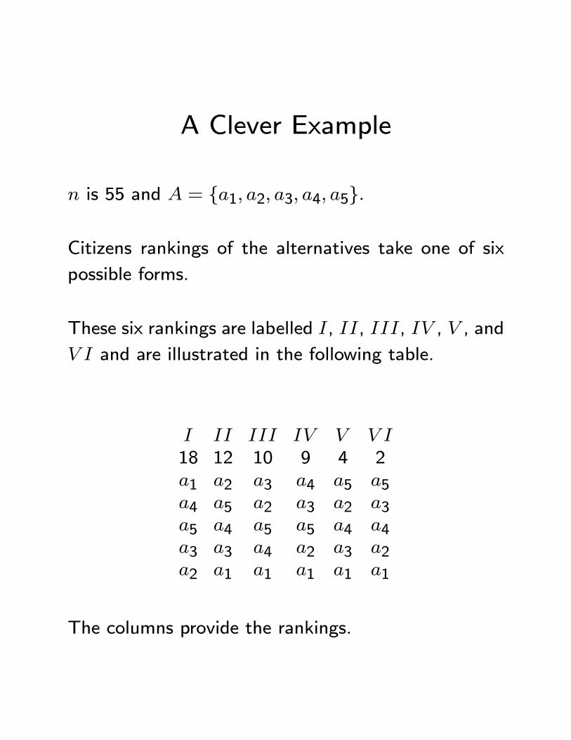
A Clever Example

is 55 and = {1 2 3 4 5}

Citizens rankings of the alternatives take one of six

possible forms.

These six rankings are labelled , , , , , and

and are illustrated in the following table.

18 12 10 9 4 2

1 2 3 4 5 54 5 2 3 2 35 4 5 5 4 43 3 4 2 3 22 1 1 1 1 1

The columns provide the rankings.

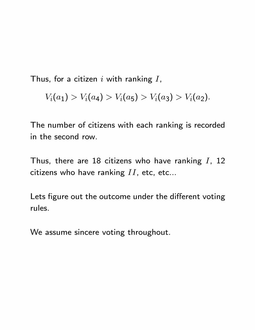
Thus, for a citizen with ranking ,

(1) (4) (5) (3) (2)

The number of citizens with each ranking is recorded

in the second row.

Thus, there are 18 citizens who have ranking , 12

citizens who have ranking , etc, etc...

Lets figure out the outcome under the different voting

rules.

We assume sincere voting throughout.

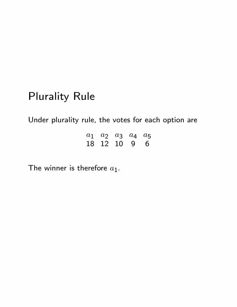
Plurality Rule

Under plurality rule, the votes for each option are

1 2 3 4 518 12 10 9 6

The winner is therefore 1.

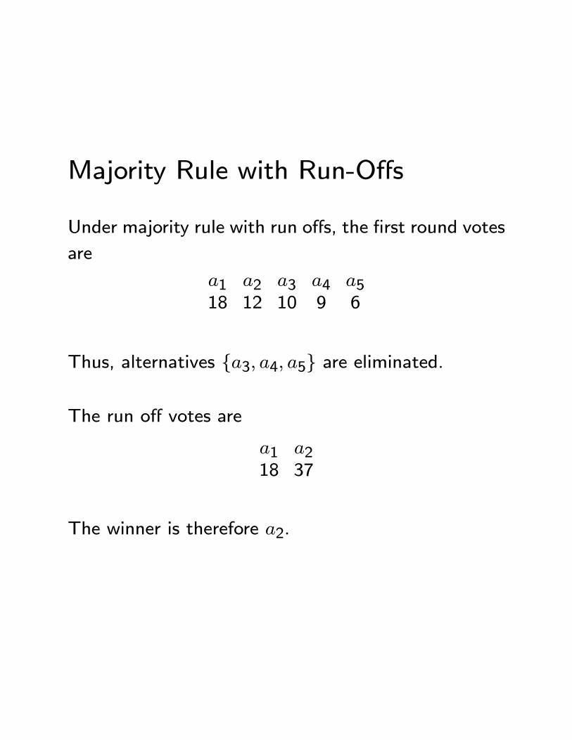
Majority Rule with Run-Offs

Under majority rule with run offs, the first round votes

are

1 2 3 4 518 12 10 9 6

Thus, alternatives {3 4 5} are eliminated.

The run off votes are

1 218 37

The winner is therefore 2.

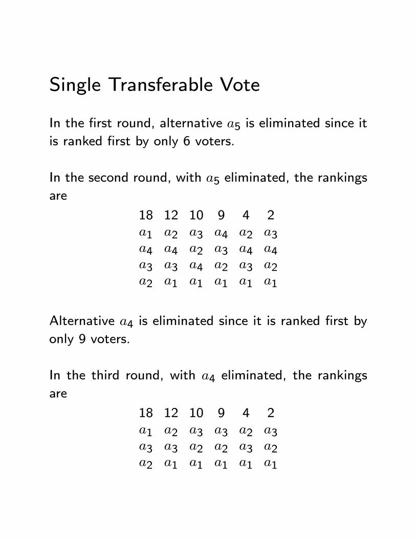
Single Transferable Vote

In the first round, alternative 5 is eliminated since it

is ranked first by only 6 voters.

In the second round, with 5 eliminated, the rankings

are

18 12 10 9 4 2

1 2 3 4 2 34 4 2 3 4 43 3 4 2 3 22 1 1 1 1 1

Alternative 4 is eliminated since it is ranked first by

only 9 voters.

In the third round, with 4 eliminated, the rankings

are

18 12 10 9 4 2

1 2 3 3 2 33 3 2 2 3 22 1 1 1 1 1

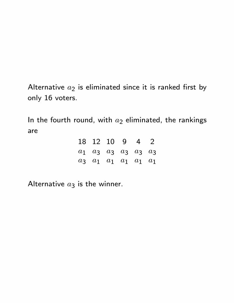
Alternative 2 is eliminated since it is ranked first by

only 16 voters.

In the fourth round, with 2 eliminated, the rankings

are

18 12 10 9 4 2

1 3 3 3 3 33 1 1 1 1 1

Alternative 3 is the winner.

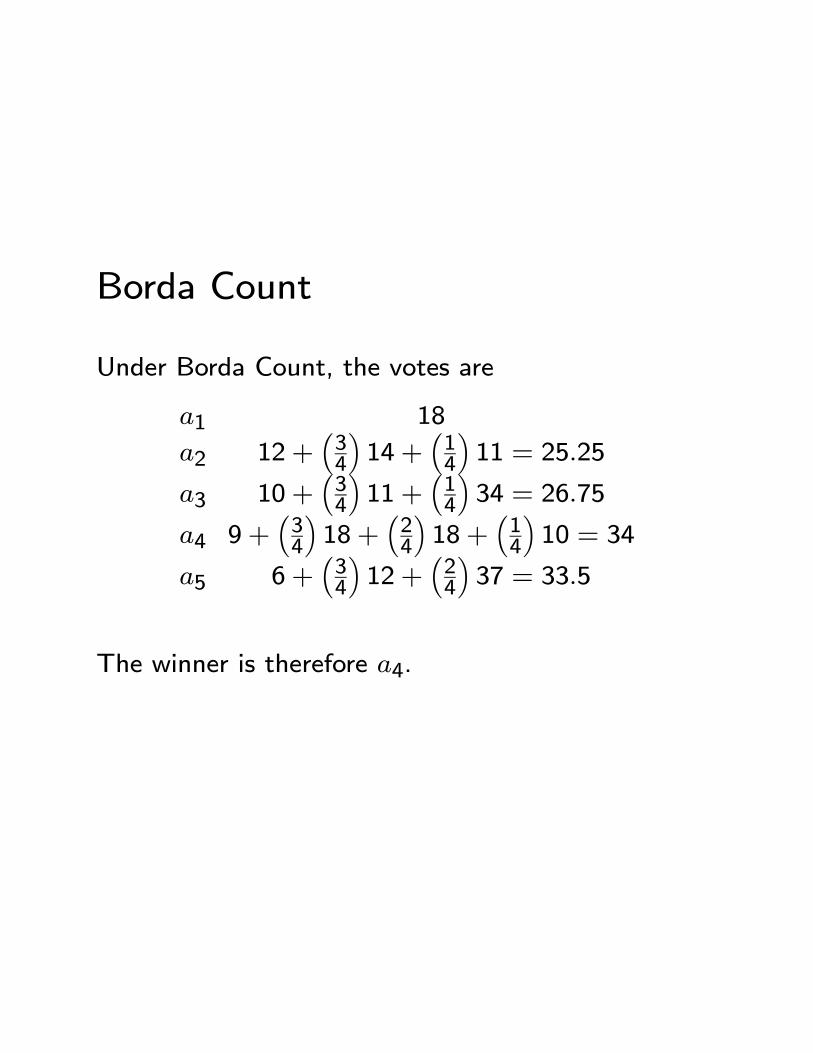
Borda Count

Under Borda Count, the votes are

1 18

2 12 +³34

´14 +

³14

´11 = 2525

3 10 +³34

´11 +

³14

´34 = 2675

4 9 +³34

´18 +

³24

´18 +

³14

´10 = 34

5 6 +³34

´12 +

³24

´37 = 335

The winner is therefore 4.

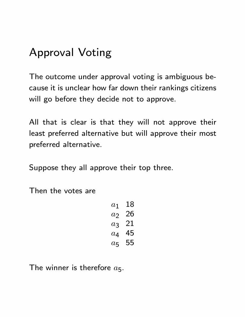
Approval Voting

The outcome under approval voting is ambiguous be-

cause it is unclear how far down their rankings citizens

will go before they decide not to approve.

All that is clear is that they will not approve their

least preferred alternative but will approve their most

preferred alternative.

Suppose they all approve their top three.

Then the votes are

1 18

2 26

3 21

4 45

5 55

The winner is therefore 5.

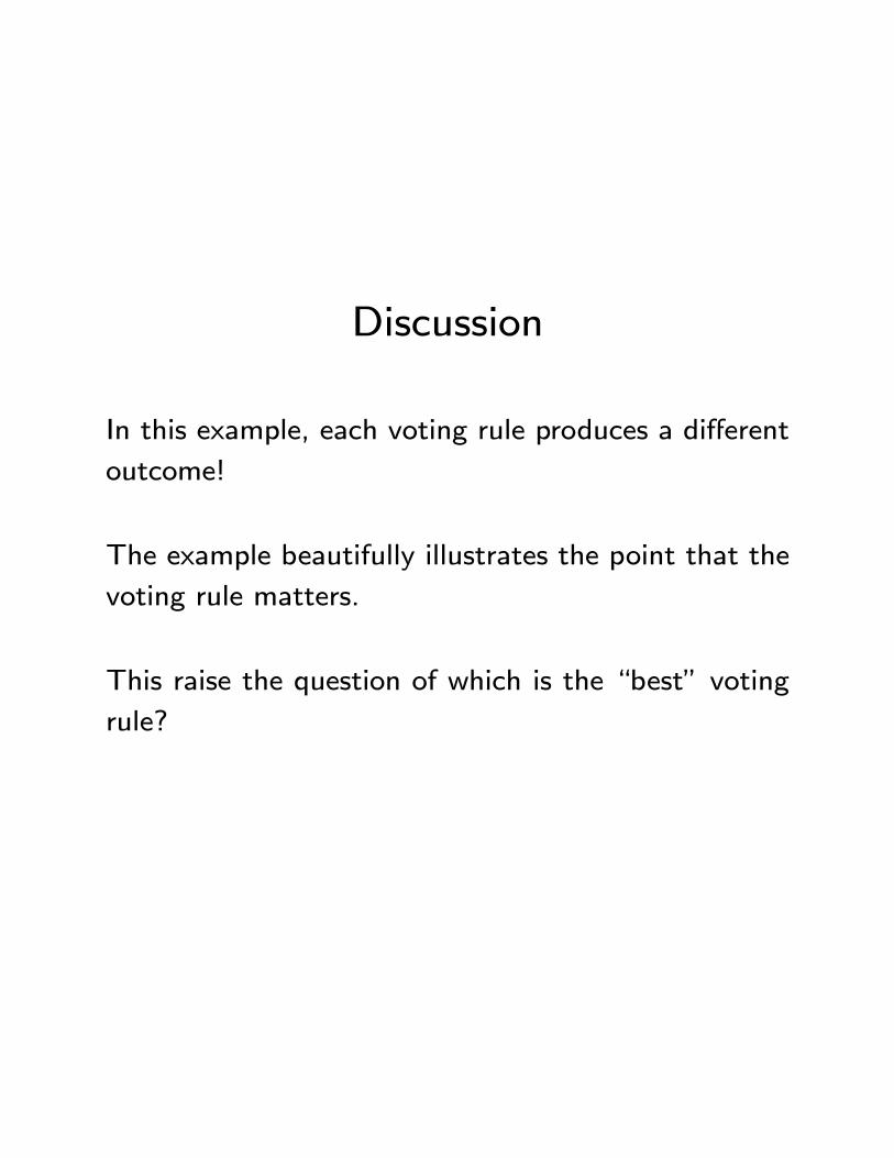
Discussion

In this example, each voting rule produces a different

outcome!

The example beautifully illustrates the point that the

voting rule matters.

This raise the question of which is the “best” voting

rule?

II.2 General Results

We now discuss two general results relating to voting

rules which are relevant for thinking about the ques-

tion of a best voting rule.

II.2.i Arrow’s Impossibility Theorem

Arrow was concerned with the problem of constructing

a social ranking of alternatives from a set of individual

rankings.

The different voting rules that we have discussed rep-

resent different ways of doing this.

They all provide ways of going from individual rank-

ings to a social ranking.

For example, in the Clever Example, the individual

rankings are those given in the initial table.

The social ranking under plurality rule is

1 Â 2 Â 3 Â 4 Â 5

where the notation  means is ranked higher than.

The social ranking under the Borda count is

4 Â 5 Â 3 Â 2 Â 1

Arrow wanted to find “good” ways of constructing

these social rankings.

Clearly, this is an interesting problem, since if we can

agree on what are good and not so good ways to

construct social rankings we may then be able to judge

between different voting rules.

The way Arrow approached the problem was to specify

a set of conditions that he thought any good method

of social ranking should satisfy.

He then proved that there was no method which sat-

isfied these conditions.

Arrow’s framework

Arrow’s underlying framework was similar to the one

we used to discuss voting rules, except that he as-

sumed that citizens simply have rankings over the al-

ternatives rather than utility functions.

Recall from micro, that rankings (or equivalently pref-

erences) are the more fundamental concept.

Utility functions are just a way of representing prefer-

ences.

Thus, we have a community with citizens indexed

by ∈ {1 }.

This community must choose some alternative from

a finite set of feasible alternatives = {1 }.

The number of alternatives is and we assume ≥3.

Each citizen has a ranking or preference over these

alternatives denoted º.

The notation º means that citizen ranks

alternative at least as high as alternative (or

equivalently weakly prefers alternative to alterna-

tive ).

The notation  means that º but that

it is not the case that º ; i.e., citizen ranks

alternative higher than alternative (or equiva-

lently strictly prefers alternative to alternative ).

We assume that each citizen ’s ranking is complete

and transitive.

Complete means that citizen can rank any two al-

ternatives.

Formally, for any two alternatives and , either

º or º .

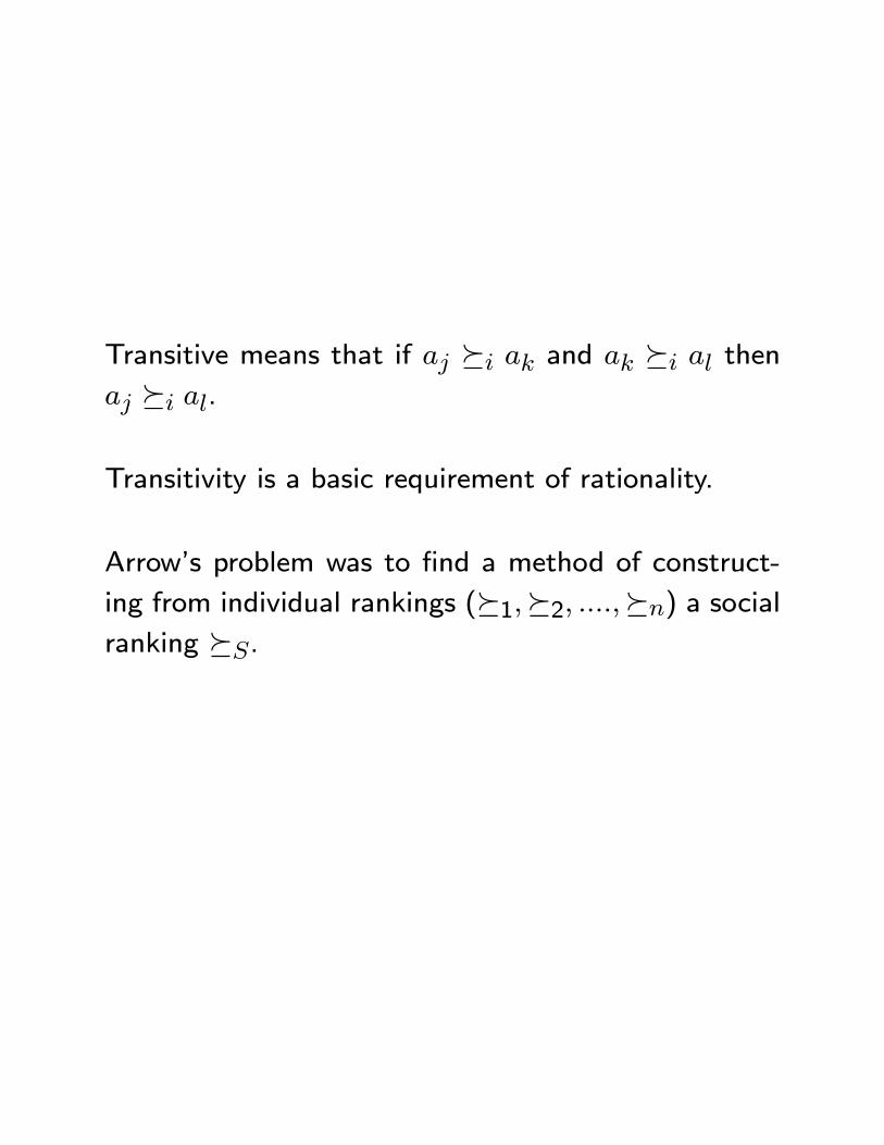
Transitive means that if º and º then

º .

Transitivity is a basic requirement of rationality.

Arrow’s problem was to find a method of construct-

ing from individual rankings (º1º2 º) a social

ranking º.

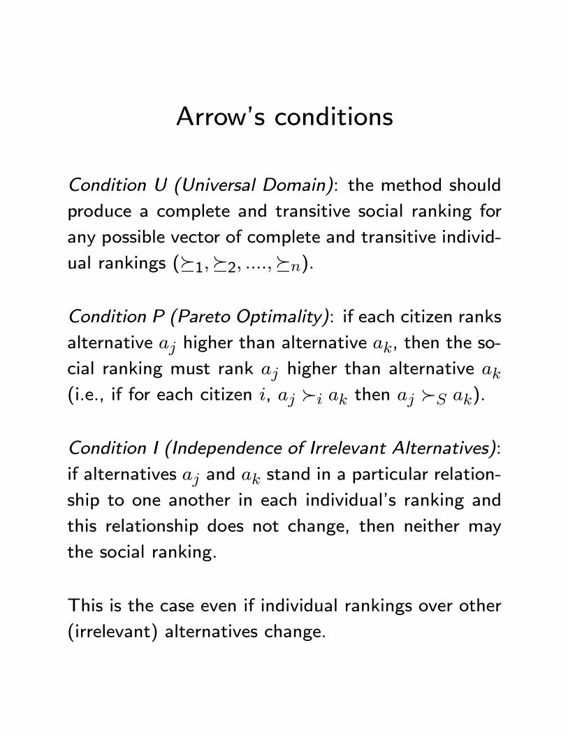
Arrow’s conditions

Condition U (Universal Domain): the method should

produce a complete and transitive social ranking for

any possible vector of complete and transitive individ-

ual rankings (º1º2 º).

Condition P (Pareto Optimality): if each citizen ranks

alternative higher than alternative , then the so-

cial ranking must rank higher than alternative

(i.e., if for each citizen ,  then  ).

Condition I (Independence of Irrelevant Alternatives):

if alternatives and stand in a particular relation-

ship to one another in each individual’s ranking and

this relationship does not change, then neither may

the social ranking.

This is the case even if individual rankings over other

(irrelevant) alternatives change.

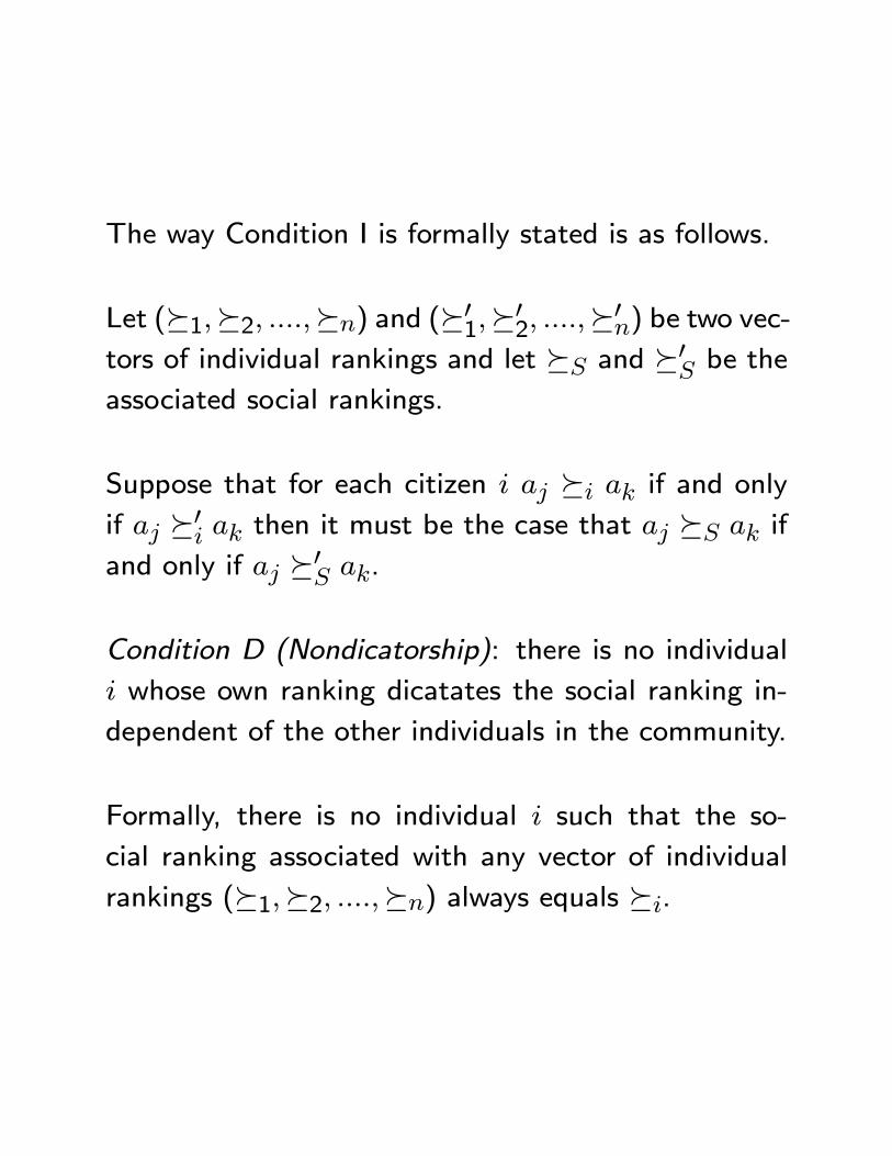
The way Condition I is formally stated is as follows.

Let (º1º2 º) and (º01º02 º0) be two vec-tors of individual rankings and let º and º0 be theassociated social rankings.

Suppose that for each citizen º if and only

if º0 then it must be the case that º if

and only if º0 .

Condition D (Nondicatorship): there is no individual

whose own ranking dicatates the social ranking in-

dependent of the other individuals in the community.

Formally, there is no individual such that the so-

cial ranking associated with any vector of individual

rankings (º1º2 º) always equals º.

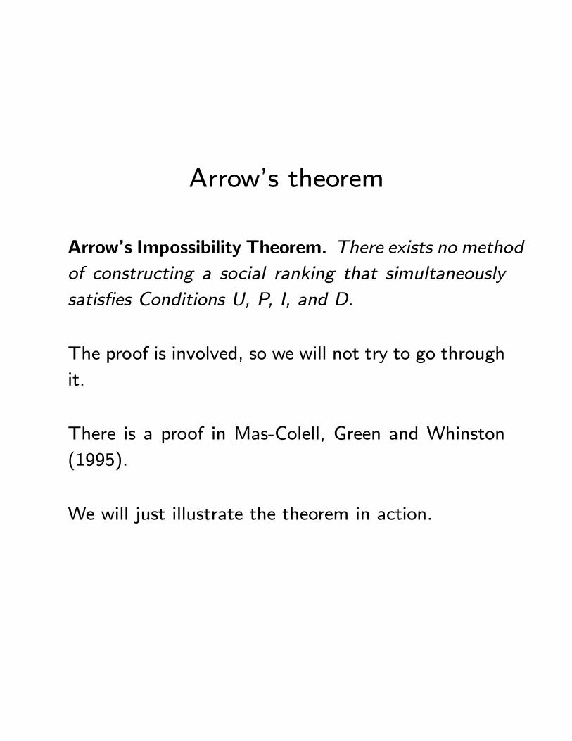
Arrow’s theorem

Arrow’s Impossibility Theorem. There exists no method

of constructing a social ranking that simultaneously

satisfies Conditions U, P, I, and D.

The proof is involved, so we will not try to go through

it.

There is a proof in Mas-Colell, Green and Whinston

(1995).

We will just illustrate the theorem in action.

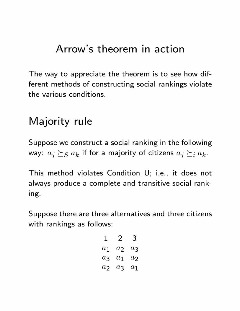
Arrow’s theorem in action

The way to appreciate the theorem is to see how dif-

ferent methods of constructing social rankings violate

the various conditions.

Majority rule

Suppose we construct a social ranking in the following

way: º if for a majority of citizens º .

This method violates Condition U; i.e., it does not

always produce a complete and transitive social rank-

ing.

Suppose there are three alternatives and three citizens

with rankings as follows:

1 2 3

1 2 33 1 22 3 1

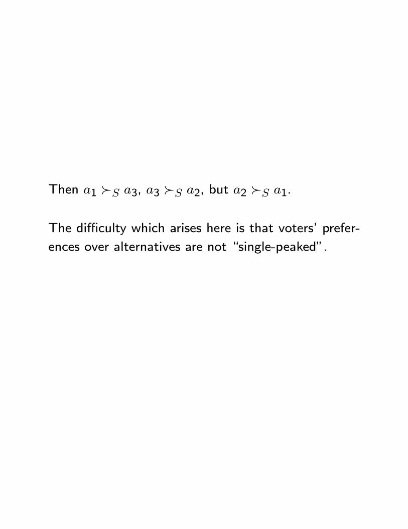
Then 1 Â 3, 3 Â 2, but 2 Â 1.

The difficulty which arises here is that voters’ prefer-

ences over alternatives are not “single-peaked”.

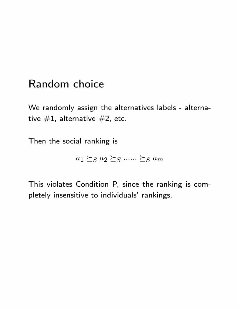
Random choice

We randomly assign the alternatives labels - alterna-

tive #1, alternative #2, etc.

Then the social ranking is

1 º 2 º º

This violates Condition P, since the ranking is com-

pletely insensitive to individuals’ rankings.

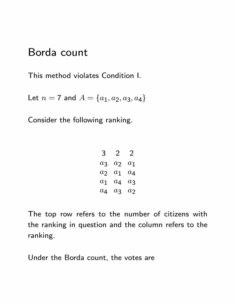
Borda count

This method violates Condition I.

Let = 7 and = {1 2 3 4}

Consider the following ranking.

3 2 2

3 2 12 1 41 4 34 3 2

The top row refers to the number of citizens with

the ranking in question and the column refers to the

ranking.

Under the Borda count, the votes are

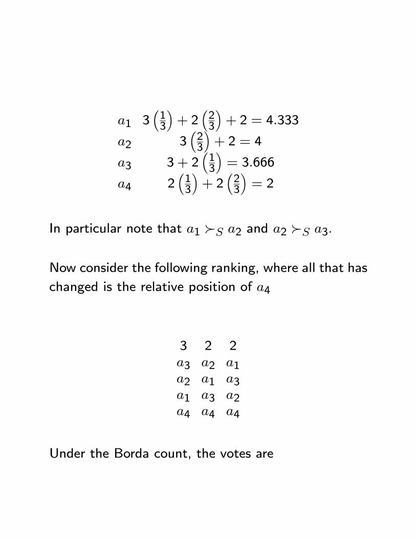
1 3³13

´+ 2

³23

´+ 2 = 4333

2 3³23

´+ 2 = 4

3 3 + 2³13

´= 3666

4 2³13

´+ 2

³23

´= 2

In particular note that 1 Â 2 and 2 Â 3.

Now consider the following ranking, where all that has

changed is the relative position of 4

3 2 2

3 2 12 1 31 3 24 4 4

Under the Borda count, the votes are

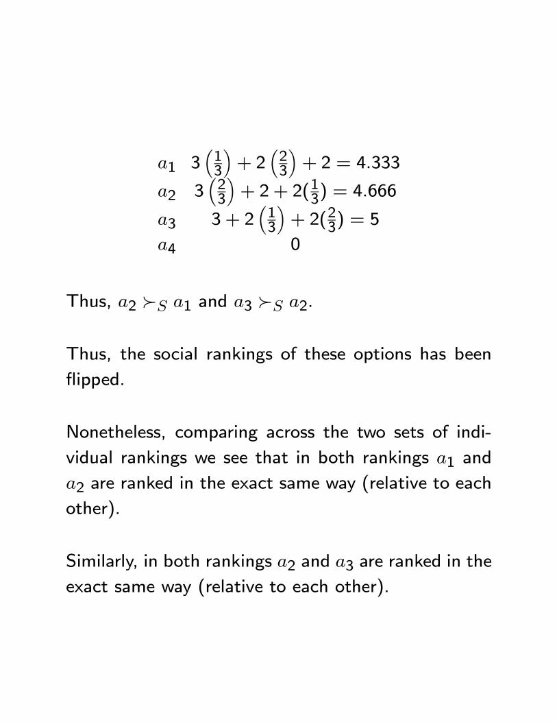
1 3³13

´+ 2

³23

´+ 2 = 4333

2 3³23

´+ 2 + 2(1

3) = 4666

3 3 + 2³13

´+ 2(23) = 5

4 0

Thus, 2 Â 1 and 3 Â 2.

Thus, the social rankings of these options has been

flipped.

Nonetheless, comparing across the two sets of indi-

vidual rankings we see that in both rankings 1 and

2 are ranked in the exact same way (relative to each

other).

Similarly, in both rankings 2 and 3 are ranked in the

exact same way (relative to each other).

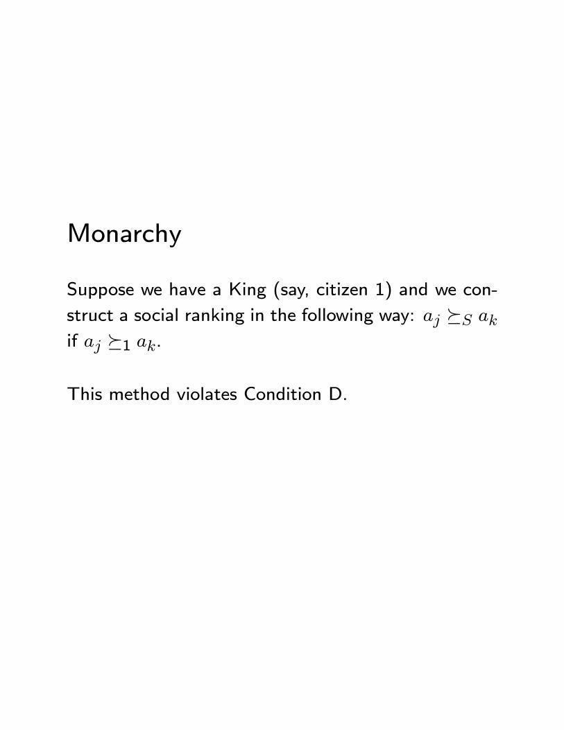
Monarchy

Suppose we have a King (say, citizen 1) and we con-

struct a social ranking in the following way: º

if º1 .

This method violates Condition D.

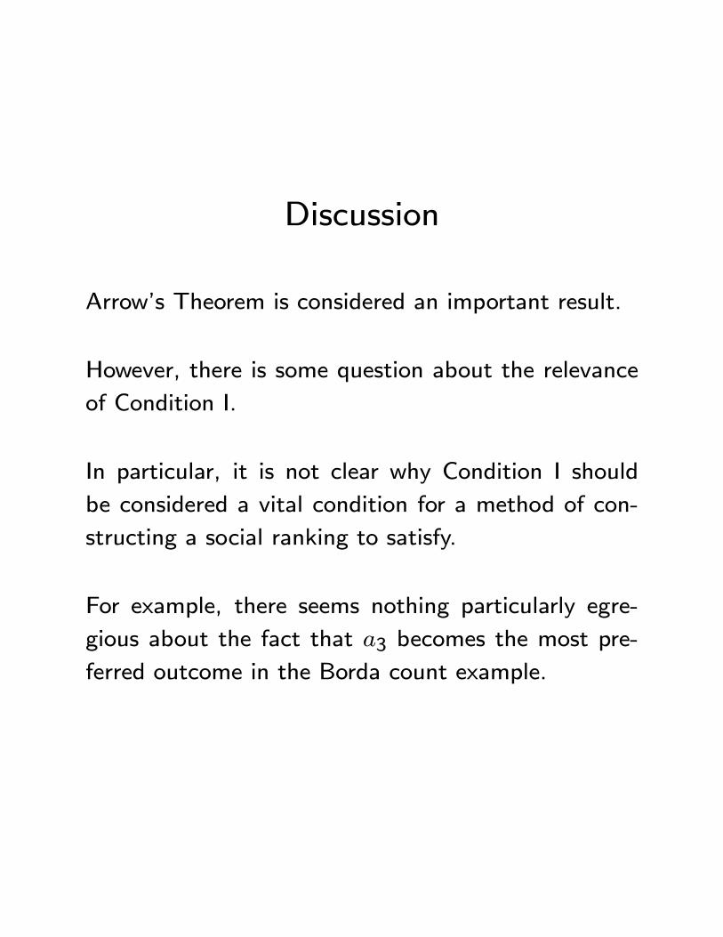
Discussion

Arrow’s Theorem is considered an important result.

However, there is some question about the relevance

of Condition I.

In particular, it is not clear why Condition I should

be considered a vital condition for a method of con-

structing a social ranking to satisfy.

For example, there seems nothing particularly egre-

gious about the fact that 3 becomes the most pre-

ferred outcome in the Borda count example.

II.2.ii Gibbard-Satterthwaite Theorem

In considering the problem of constructing a social

ranking of alternatives from a set of individual rank-

ings, Arrow implicitly assumed that individuals would

report their true rankings accurately.

However, it is fairly obvious that in some circum-

stances individuals will have an incentive to misreport

their rankings.

Lets consider two motivating examples.

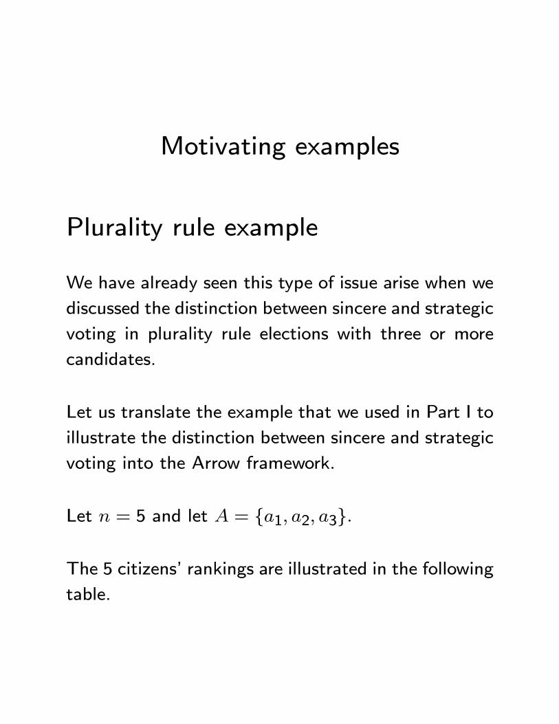
Motivating examples

Plurality rule example

We have already seen this type of issue arise when we

discussed the distinction between sincere and strategic

voting in plurality rule elections with three or more

candidates.

Let us translate the example that we used in Part I to

illustrate the distinction between sincere and strategic

voting into the Arrow framework.

Let = 5 and let = {1 2 3}

The 5 citizens’ rankings are illustrated in the following

table.

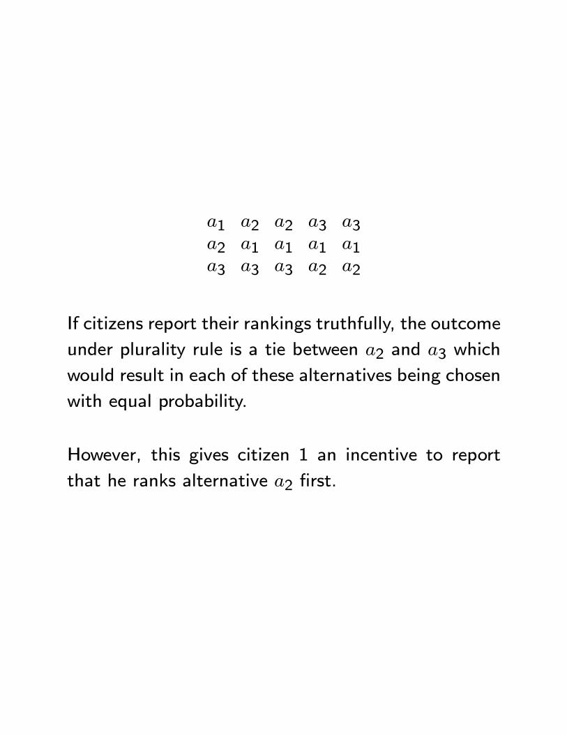
1 2 2 3 32 1 1 1 13 3 3 2 2

If citizens report their rankings truthfully, the outcome

under plurality rule is a tie between 2 and 3 which

would result in each of these alternatives being chosen

with equal probability.

However, this gives citizen 1 an incentive to report

that he ranks alternative 2 first.

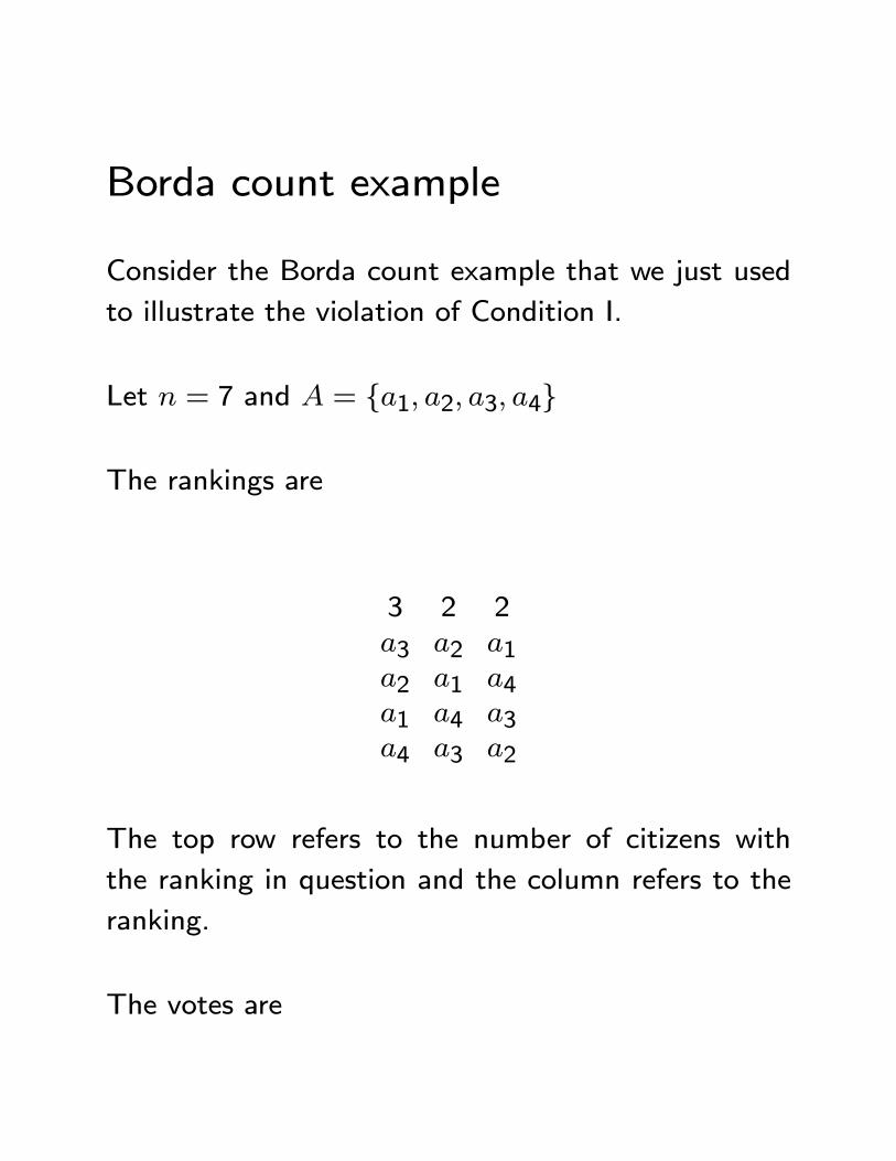
Borda count example

Consider the Borda count example that we just used

to illustrate the violation of Condition I.

Let = 7 and = {1 2 3 4}

The rankings are

3 2 2

3 2 12 1 41 4 34 3 2

The top row refers to the number of citizens with

the ranking in question and the column refers to the

ranking.

The votes are

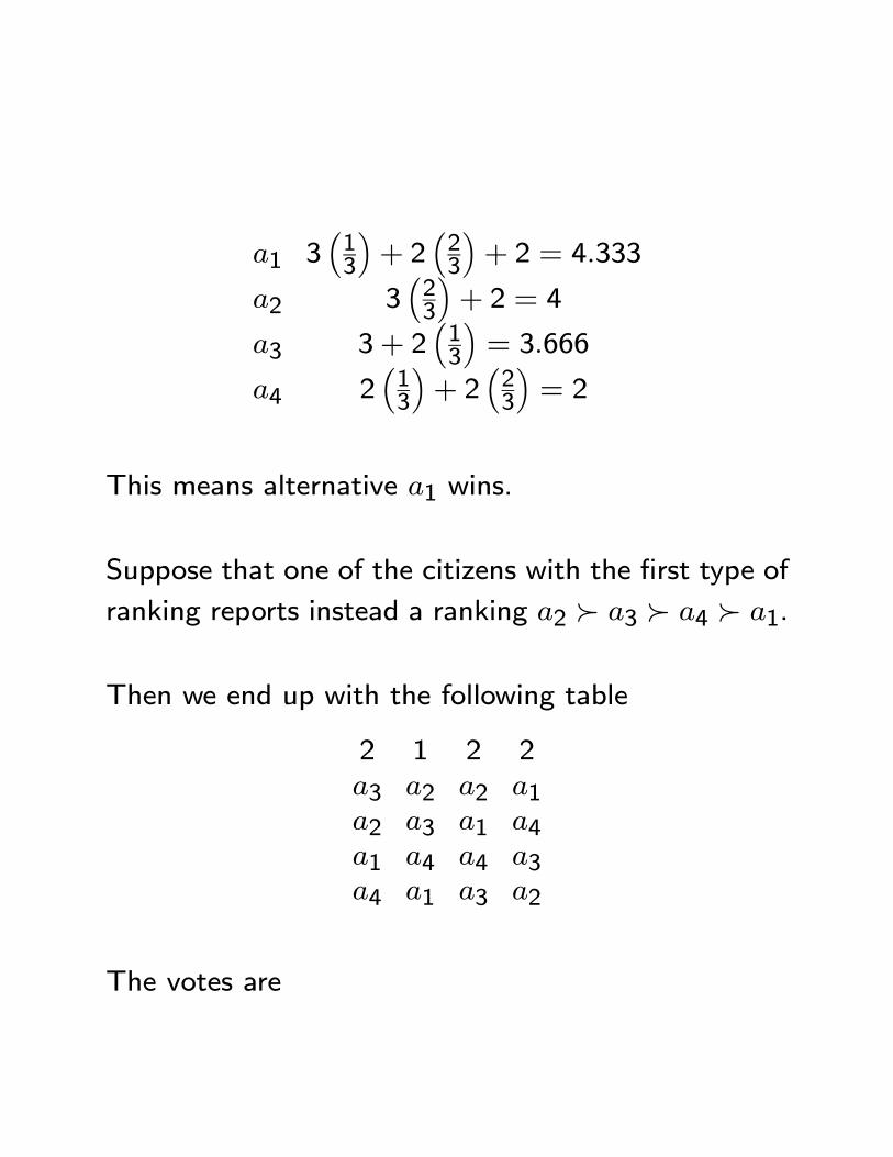
1 3³13

´+ 2

³23

´+ 2 = 4333

2 3³23

´+ 2 = 4

3 3 + 2³13

´= 3666

4 2³13

´+ 2

³23

´= 2

This means alternative 1 wins.

Suppose that one of the citizens with the first type of

ranking reports instead a ranking 2 Â 3 Â 4 Â 1.

Then we end up with the following table

2 1 2 2

3 2 2 12 3 1 41 4 4 34 1 3 2

The votes are

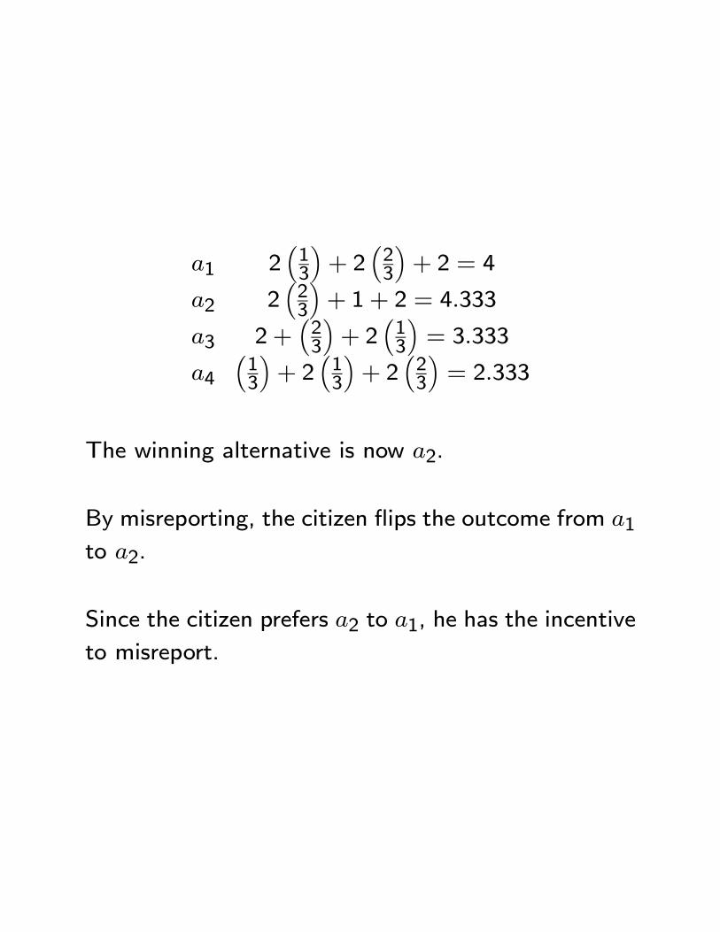
1 2³13

´+ 2

³23

´+ 2 = 4

2 2³23

´+ 1 + 2 = 4333

3 2 +³23

´+ 2

³13

´= 3333

4

³13

´+ 2

³13

´+ 2

³23

´= 2333

The winning alternative is now 2.

By misreporting, the citizen flips the outcome from 1

to 2.

Since the citizen prefers 2 to 1, he has the incentive

to misreport.

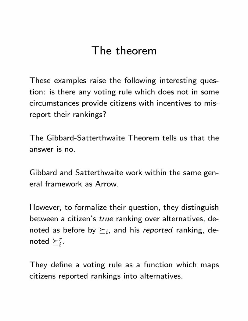
The theorem

These examples raise the following interesting ques-

tion: is there any voting rule which does not in some

circumstances provide citizens with incentives to mis-

report their rankings?

The Gibbard-Satterthwaite Theorem tells us that the

answer is no.

Gibbard and Satterthwaite work within the same gen-

eral framework as Arrow.

However, to formalize their question, they distinguish

between a citizen’s true ranking over alternatives, de-

noted as before by º, and his reported ranking, de-

noted º .

They define a voting rule as a function which maps

citizens reported rankings into alternatives.

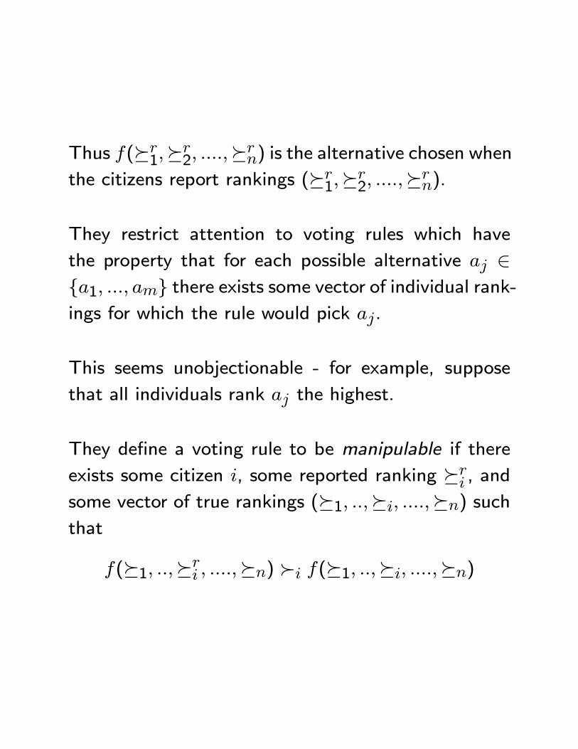
Thus (º1º

2 º) is the alternative chosen when

the citizens report rankings (º1º

2 º).

They restrict attention to voting rules which have

the property that for each possible alternative ∈{1 } there exists some vector of individual rank-ings for which the rule would pick .

This seems unobjectionable - for example, suppose

that all individuals rank the highest.

They define a voting rule to be manipulable if there

exists some citizen , some reported ranking º , and

some vector of true rankings (º1 º º) such

that

(º1 º º) Â (º1 º º)

Intuitively, when the true rankings are (º1 º º

) citizen gains from reporting the ranking º rather

than reporting his true ranking º when everyone else

reports their true ranking.

In game-theoretic language, if a voting rule is manip-

ulable, reporting truthfully is not a dominant strategy

equilibrium for some vector of true rankings.

Finally, they define a voting rule to be dictatorial if

there exists some citizen such that whatever the cit-

izens report, the voting rule always chooses the out-

come that citizen ranks highest.

Gibbard-Satterthwaite Theorem. Every non-dictatorial

voting rule is manipulable.

Discussion

The Gibbard-Satterthwaite Theorem is considered im-

portant in the literature.

The point seems unobjectionable - any voting rule is

going to sometimes give people an incentive to mis-

report their preferences.

The point is arguably not so surprising, but the way

the problem is formalized is nice and paved the way

for the mechanism design literature.

II.2.iii Further work on voting rules

The two general results we have described are both

negative results.

Arrow’s theorem tells us that any voting rule will for

some configurations of citizens’ preferences produce

what are arguably pathological results.

Gibbard and Satterthwaite’s theorem tells us that any

voting rule will for some configurations of citizens’

preferences provide incentives to vote in a way that

does not reflect their sincere preferences.

The results are often interpreted as suggesting that

there is no best voting rule and that it is sort of point-

less to look for one.

Nonetheless, communities must choose the rules that

they will use to decide and hence the question still

remains as to which one should they choose.

More recent literature has tried to be more practically

orientated and compare the relative merits of different

voting rules.

Cox (1987) considers Downsian competition between

an exogenous number (3 or more) of candidates and

provides a comparison of various voting rules.

He shows that there are no symmetric equilibria under

plurality rule, but with the Borda count there exists a

unique symmetric equilibrium in which all candidates

adopt the position of the median voter.

Myerson (1999) argues that plurality rule provides can-

didates with greater incentive to create programs that

transfer resources to small minorities of voters than do

rules like Borda count.

These analyses assume: (i) sincere voting; (ii) Down-

sian candidates; and (iii) a fixed number of candidates.

Myerson (1999) also compares plurality rule and ap-

proval voting with strategic voting and three Down-

sian candidates.

He shows that approval voting yields median out-

comes, while plurality rule need not.

The problem is coordination failure among voters stem-

ming from the wasted vote idea.

Osborne and Slivinski (1996) compare outcomes un-

der plurality rule and majority rule with run-offs in a

citizen-candidate model with sincere voting.

They find that two candidate elections are “more likely”

under plurality rule and that candidates’ positions are

“less differentiated” under majority rule with run-offs.

Dellis and Oak (2003) compare outcomes under plu-

rality rule and approval voting in a citizen-candidate

model with strategic voting.

Interestingly, they find that approval voting is capable

of generating similar anomalies to plurality rule.

They do, however, present conditions under which ap-

proval voting leads to more moderate outcomes.

Comparison of voting rules is an important area of

ongoing research.

There is plenty of comparisons to do, but results are

hard to find.

II.3 Electoral systems

To this point, we have focused on methods commu-

nities can use to choose a single alternative.

We now broaden the discussion to consider methods

to choose a legislature.

If we have single-seat districts (as in U.S. congres-

sional districts), we just need to elect a single candi-

date in each district and we can use any of the voting

rules that we have already discussed.

Matters get more complicated if we have multi-seat

districts.

In some countries, for example, the whole country

elects the whole legislature (Isreal and the Nether-

lands) so there is only one district!

Suppose that we have to elect ≥ 2 candidates froma district.

Single non-transferable vote

The simplest system would be the single non-transferable

vote.

Under this system, citizens have one vote to cast and

the candidates with the most votes are elected.

This system is used in Japan for the lower house,

where each district has three to five seats.

While this system generalizes plurality rule, it creates

new strategic issues - for example, citizens may not

cast their vote for the candidate they like most if they

think he is already going to be in the top .

In addition, political parties face a difficult choice in

knowing how many candidates to put up - a large

party may end up with few seats if it puts up too

many candidates and voters split their votes among

them.

Limited vote

A variant of this system is the limited vote, under

which each citizen has votes (where is between

2 and ) and the candidates with the most votes

are elected.

For example, in a district with four seats, voters may

be allowed to vote for two candidates.

This system is used in local elections in the U.S. and

also to elect the senate in Spain.

Single transferable vote

The single transferable vote system discussed above

can be generalized to handle multi-seat districts.

It is used by Ireland and Malta to elect representatives

to their lower houses - they have districts with three

to five seats.

One needs to define a quota of first place votes

above which any candidate gets a seat and also a

transfer rule by which a winning candidate’s surplus

is redistributed to the other candidates.

We go through the same procedure as described in

Part II.1 until we find the first candidate who has

more than first place votes in the set of uneliminated

candidates.

This candidate then takes one of the seats and is elim-

inated.

If his first place votes were then his surplus votes

− must be redistributed to the other candidates.

Suppose that candidate is in second place on of

these ballots.

Then, in the next round he is awarded (−) first

place votes.

The weighting ensures that the sum of all candidates’

scores remains equal to the total number of votes cast.

To illustrate, suppose we have 3 candidates, , , &

, 100 voters, and 2 seats.

We set = 34.

Suppose that the voters rankings are

50 25 25

Then, A is elected in the first round and his surplus is

50− 34 = 16.

Thus, the second round votes are 25 + 50(1650) for B

and 25 for C.

B is then elected in the second round.

The single transferable vote system is very compli-

cated and not practical in circumstances in which vot-

ers are electing many representatives.

In such circumstances, the most common electoral

system is some form of proportional representation

(PR).

Proportional representation

When candidates are put forward by competing polit-

ical parties, List-PR systems are common.

Under these systems, the alternatives on the ballot are

lists of candidates, each list associated with a different

party.

List PR systems differ in terms of whether citizens can

vote for candidates or for parties.

In a closed-list PR system, citizens can vote only for

parties and then seats are allocated to parties in pro-

portion to their vote share.

If, say, Party A gets 10 seats then the first 10 candi-

dates on Party A’s list are allocated these seats.

Each party chooses the order in which to list candi-

dates.

This gives party leadership a large amount of power

and gives rise to strong parties (as defined in Part I.5).

The way the seats are allocated among parties is straight-

forward.

For example, suppose that we have a five seat district,

five parties compete and the percent vote distribution

among them is 48.5-29-14-7.5-1.

The quota required for a seat is 20%.

The largest party is allocated two seats and this leaves

a surplus of 8.5.

The second largest party is allocated one seat and this

leaves a surplus of 9.

The remaining two seats are allocated to the third

party and the second party - so the overall seat distri-

bution is 2-2-1-0-0

In an open-list PR system, citizens can not only vote

for parties but also which candidates from a party’s

list they prefer.

For example, in Belgium, the candidates are listed on

the ballot and the voter places an optional ”x” by

his/her preferred candidates.

The rules then specify what percentage of votes cast

a candidate must have in individual preferences to be

moved up the list.

In this way, open-list PR allows voters to change the

order in which party leaders have ranked candidates.

II.4 Comparing electoral systems

It is obviously interesting to think about the outcomes

that different systems produce.

There is a huge political science literature devoted to

this task.

A major focus is the comparison of proportional rep-

resentation with plurality rule.

Under the former parties receive seat shares propor-

tional to their votes and under the latter the party

with the most votes in each district gets the seat.

There are two general claims commonly made about

these systems.

Claim 1: number of parties

The first claim is that plurality rule leads to two party

competition, while proportional representation leads

to multiple parties.

This is known as Duverger’s Law.

The logic underlying this claim is based on the idea of

voters not wanting to waste their votes by voting for

small parties under plurality rule.

This logic showed up in our discussion of why it could

be an equilibrium for two extremist candidates to run

against each other in the citizen-candidate model.

Under proportional representation, seats are propor-

tional to votes and hence voting for a small party does

not lead to a wasted vote.

Indeed, in proportional representation systems, small

parties can have large influence if they form part of

the governing coalition.

There is some evidence for this claim - there do tend

to be less political parties in plurality rule systems and,

in some instances (such as the U.S.) there are just two

main parties.

Claim 2: types of policies

The second claim is that plurality rule provides parties

with more incentive to use tax dollars to implement

narrowly targeted transfer programs rather than pro-

viding universally valued public programs.

The logic behind this prediction is that plurality rule

gives rise to a discontinuous relationship between seats

and votes, whereby a party can get a whole lot more

seats if it can increase its vote share to just slightly

more than its closest rival.

This makes it highly valuable to attract the votes of

small constituencies and hence leads to an abundance

of special programs designed to appeal to small con-

stituencies.

By contrast, in proportional representation systems,

the relationship between seats and votes is continuous.

There is also some evidence for this claim: spending

on broadly targeted social programs tends to be higher

in proportional representation systems.

Related formal models

Lizzeri and Persico (2001) is an effort to come up with

a formalization of Claim 2.

They study two-party competition for legislative seats

under plurality rule (the party with the most votes gets

all the seats) and proportional representation (seats

are awarded in proportion to votes).

They show that plurality rule provides parties with

more incentive to use tax dollars to implement nar-

rowly targeted transfer programs rather than providing

a universally valued public good.

One limitation of Lizzeri and Persico is their model of

proportional representation assumes two parties.

One might imagine that if proportional representation

systems allows more parties, then some of the small

parties might represent small constituencies.

In general, progress on modelling policy formation in

PR systems with many parties has been quite limited.

Baron and Diermier (2001) present an interesting model

of elections and government formation in PR systems.

Their model has three policy-motivated parties.

Parties cannot commit and voters must anticipate the

possible formation of a coalition government if one

party does not have a majority of seats.

Government formation is modelled as a bargaining

process.

Morelli (2004) undertakes the even more ambitious

task of trying to compare both policy choice and party

formation under plurality rule and proportional repre-

sentation.

One of his goals is to try and formalize Claim 2.

His model incorporates strategic voters, strategic can-

didates, and strategic parties.

In fact, he does not find consistent results in terms of

which system has the most parties, but proportional

representation produces more centrist policies under

some conditions.

Again, using formal models to explore the implica-

tions of different systems and testing their predictions

empirically is an active area of research.

For more work in this style see Coate and Knight

(2011), Persson, Roland, and Tabellini (2000), and

Persson and Tabellini’s book chapter in W & W.

III. Political Distortions

An important goal of public choice theory is to un-

derstand how political decision-making distorts policy

choices away from those choices that would be made

by the benevolent governments from economics text-

books.

Such governments intervene to correct market failures

and to redistribute income to improve some appropri-

ate notion of equity.

To the extent that policies emerging from the polit-

ical process are similar to those that would be cho-

sen by benevolent governments, it is not necessary to

study politics: the prescriptions of normative theories

of government can simply be interpreted as positive

predictions.

There is a tradition in economics along these lines and

so economists interested in politics have long been

interested in understanding political distortions.

In these lectures we first briefly review some key con-

cepts from the normative study of economic policy-

making.

We then identify ways in which policies emerging from

the political process may violate standard notions of

equity.

Next we discuss reasons why politically-determined

policies may be inefficient.

Finally, we discuss the implications of political distor-

tions for the role of government.

III.1 Socially Optimal Policies

Consider a community with citizens indexed by ∈{1 }.

Suppose that this community must choose some pol-

icy from a set of feasible policies .

Citizen ’s utility if policy is selected is ().

What would be a good policy for this community?

III.1.i Pareto efficiency

The simplest requirement is that the policy be Pareto

efficient.

Formally, a policy ∗ is Pareto efficient if (i) it is fea-sible and (ii) there exists no alternative feasible policy

such that () ≥ (∗) for each citizen with the

inequality holding strictly for at least one citizen.

As a requirement for a good policy, Pareto efficiency

is certainly something that we would want.

The problem with Pareto efficiency is that a lot of

policies can be Pareto efficient, so the requirement

does not really narrow the field much.

Diagrammatic representation

Pareto efficient policies can be represented graphically

in a two person community.

The utility possibility set is the set

{(1() 2()) : ∈ }

The utility possibility frontier is the outer envelope of

this set.

Any point on the utility possibility frontier is associ-

ated with a Pareto efficient policy.

III.1.ii Social welfare functions

To go beyond the idea of Pareto efficiency, we have

to be willing to make interpersonal comparisons of

citizens’ utilities.

That is, we have to be able to compare gains and

losses of utility across citizens.

This is done with a social welfare function.

A social welfare function is a function which tells us

for any given vector of citizen utility levels what the

level of “social welfare” will be.

Mathematically, a social welfare function is represented

as a real-valued function defined over citizens’ utilities

(1 ).

Types of social welfare functions

The best known social welfare function is the Utilitar-

ian social welfare function which is

(1 ) =X

This assumes social welfare is just the sum of individ-

ual citizens’ utilities.

Another famous social welfare function is the Rawlsian

social welfare function which is

(1 ) = min

This assumes social welfare is the utility of the worst

off individual in society.

A useful social welfare function that encompasses these

two as special cases is the Iso-elastic social welfare

function which is

(1 ) =1

1−

X

1−

where is a positive constant.

When = 0, this just equals the Utilitarian social

welfare function.

As gets bigger and bigger, the Iso-elastic social wel-

fare function approaches the Rawlsian social welfare

function.

Diagrammatic representation

Social welfare functions can be represented graphically

with Social Indifference Curves.

In a two-person economy, a social indifference curve is

the set of utility pairs (1 2) satisfying the equation

(1 2) = for some constant .

By varying the constant we trace out a family of

social indifference curves.

The Utilitarian social welfare function has indifference

curves which are downward sloping straight lines, slop-

ing left to right at a 45 angle.

The Rawlsian social welfare function has L-shaped in-

difference curves which kink at the 45 line.

The Iso-elastic social welfare function has convex in-

difference curves which lie between those of the Util-

itarian and Rawlsian social welfare functions.

III.1.iii Socially optimal policies

Socially optimal policies are those that maximize so-

cial welfare as measured by the social welfare function.

Once we have agreed upon a social welfare function,

we obtain the socially optimal policy (or policies) by

solving the problem

max (1() ())

∈

Diagrammatically, the socially optimal policy is that

associated with the point at which the social indiffer-

ence curve is tangent to the utility possibility frontier.

Socially optimal policies are not only Pareto efficient

but also allocate utility optimally across citizens.

What allocating utility optimally means will depend

upon the social welfare function.

Thus, the socially optimal policy will depend on the

specific social welfare function.

III.1.iv Political distortions

Political decision-making is going to lead the commu-

nity to select some equilibrium policy and this policy

will generate some utility allocation for the citizens.

Political distortions arise when the equilibrium policy

diverges from the socially optimal policy.

There are two distinct types of distortions.

The first are political inefficiencies or political failures

in which the equilibrium policy is not even Pareto ef-

ficient.

The second are political inequities in which the equi-

librium policy is Pareto efficient but not socially opti-

mal.

III.2 Politics and Equity

We begin by discussing political inequities.

It is easy to see that politically determined policies

need not be socially optimal according to commonly

used social welfare functions.

Recall our discussion of legislatures, which is where

most policy issues are determined.

We saw that for ideological policy issues, such as the

aggregate level of spending on a policy, or the scale

of some regulation, the policy preferred by the median

legislator would be likely to be chosen.

To the extent that the median legislator’s preferences

reflects the median citizen’s preferences (for example,

as in the Downsian model), this suggests that on ide-

ological policy issues, politically determined policies

will reflect the preferences of the median citizen.

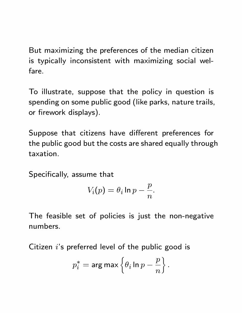
But maximizing the preferences of the median citizen

is typically inconsistent with maximizing social wel-

fare.

To illustrate, suppose that the policy in question is

spending on some public good (like parks, nature trails,

or firework displays).

Suppose that citizens have different preferences for

the public good but the costs are shared equally through

taxation.

Specifically, assume that

() = ln −

The feasible set of policies is just the non-negative

numbers.

Citizen ’s preferred level of the public good is

∗ = argmax½ ln −

¾

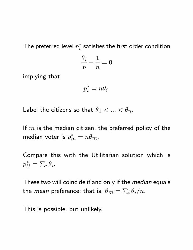
The preferred level ∗ satisfies the first order condition

− 1

= 0

implying that

∗ =

Label the citizens so that 1 .

If is the median citizen, the preferred policy of the

median voter is ∗ = .

Compare this with the Utilitarian solution which is

∗ =P .

These two will coincide if and only if themedian equals

the mean preference; that is, =P .

This is possible, but unlikely.

Stark divergencies between the two solutions arise when

there are differences in intensity of preferences.

The median solution is completely independent of how

strong the preferences are of those citizens below and

above the median.

Practically speaking, these problems arise most clearly

when society is dealing with issues in which those with

the minority view feel most strongly about the issue.

Good examples might be gay marriage, affirmative ac-

tion, and immigration reform.

It may be that interest group activity may partially

resolve these issues along the lines suggested by the

common agency model.

Nonetheless, as we pointed out, there is no particularly

good reason to suppose that interest groups will form

when there is demand for them.

When it comes to distributive policy issues, there is

even less reason to believe that outcomes will be eq-

uitable.

As we saw in the legislative bargaining model, pro-

posers get extra benefits and benefits are shared by

minimum winning coalitions.

Socially optimal policies, by contrast, will typically in-

volve equal division.

III.2.i Politically determined incomeredistribution

Just pointing out that politically determined policies

may not be socially optimal only takes us so far.

A deeper question is what determines how income gets

redistributed in political systems.

There is a large literature on this which is surveyed in

the chapter by Londregan in W & W.

We will discuss a couple of the classic papers in this

literature: Meltzer and Richards (1981) and Lindbeck

and Weibull (1987).

Meltzer and Richard’s Model

There are a continuum of individuals and two goods

- consumption and leisure.

Individuals get utility from consumption and work

according to the utility function

− (1+1)

1 +

where 0 is the elasticity of labor supply.

Individuals differ in their income generating ability.

An individual with ability earns income = if he

works an amount .

The range of ability levels is [min max].

Let () denote the fraction of individuals with ability

less than or equal to .

Let denote the median ability and let denote

the mean ability.

The government taxes income at rate and redistrib-

utes the revenue via a uniform transfer .

In reality, this uniform grant is supposed to correspond

to public programs with universal benefits like the so-

cial security system.

Given the tax rate , an individual with ability works

an amount

∗(; ) = argmax(1− )− (1+1)

1 + = ((1− ))

Note that work effort is decreasing in the tax rate.

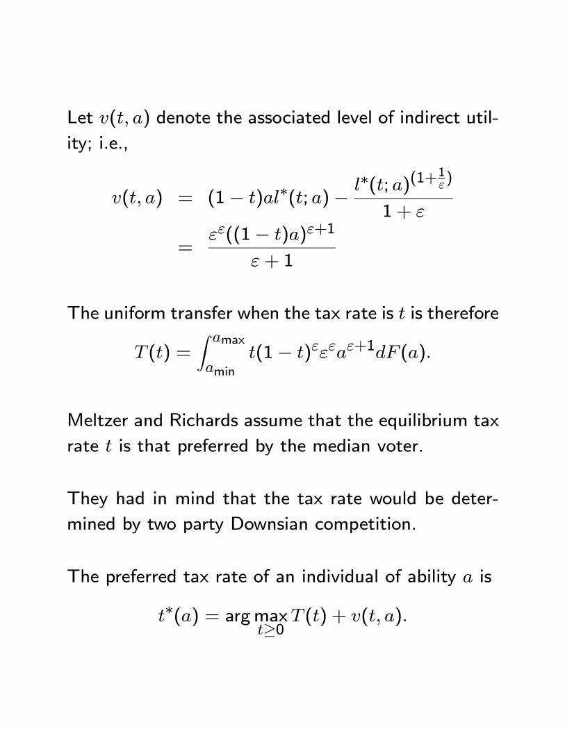
Let ( ) denote the associated level of indirect util-

ity; i.e.,

( ) = (1− )∗(; )− ∗(; )(1+1)

1 +

=((1− ))+1

+ 1

The uniform transfer when the tax rate is is therefore

() =

Z max

min(1− )+1 ()

Meltzer and Richards assume that the equilibrium tax

rate is that preferred by the median voter.

They had in mind that the tax rate would be deter-

mined by two party Downsian competition.

The preferred tax rate of an individual of ability is

∗() = argmax≥0

() + ( )

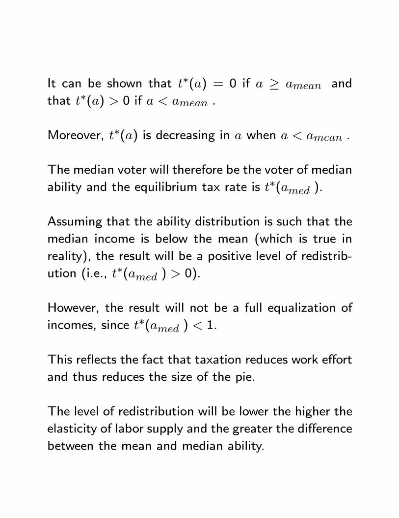
It can be shown that ∗() = 0 if ≥ and

that ∗() 0 if .

Moreover, ∗() is decreasing in when .

The median voter will therefore be the voter of median

ability and the equilibrium tax rate is ∗( ).

Assuming that the ability distribution is such that the

median income is below the mean (which is true in

reality), the result will be a positive level of redistrib-

ution (i.e., ∗( ) 0).

However, the result will not be a full equalization of

incomes, since ∗( ) 1.

This reflects the fact that taxation reduces work effort

and thus reduces the size of the pie.

The level of redistribution will be lower the higher the

elasticity of labor supply and the greater the difference

between the mean and median ability.

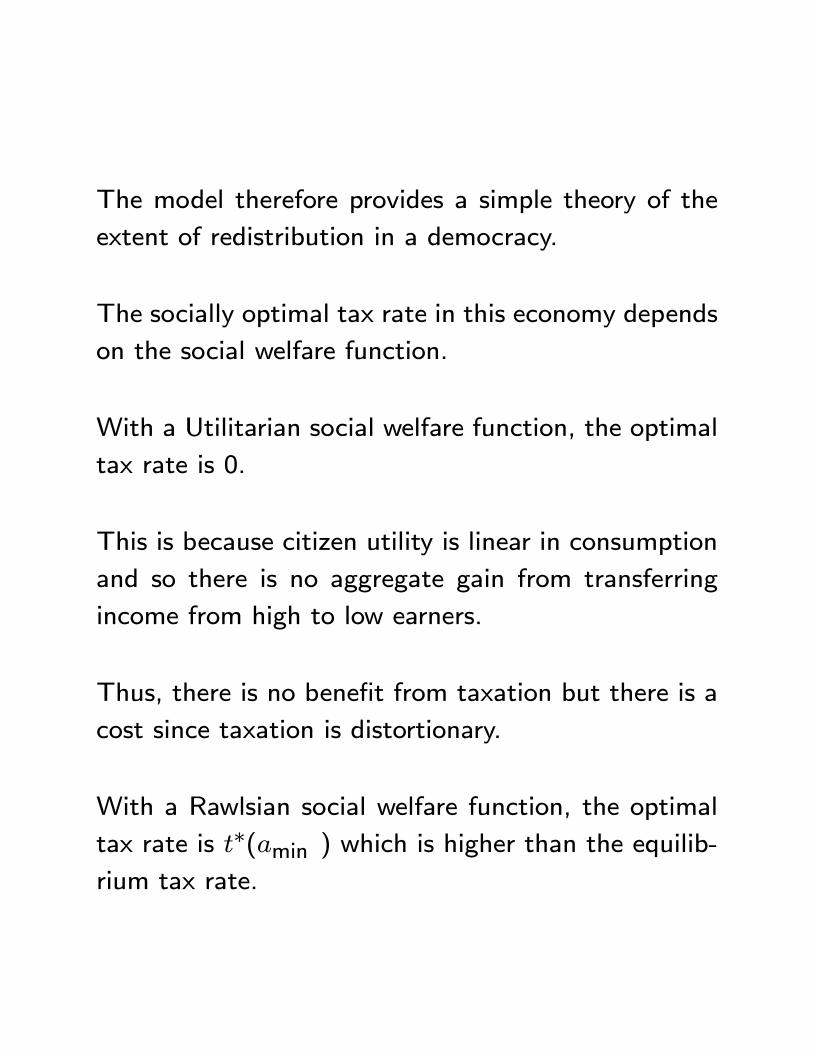
The model therefore provides a simple theory of the

extent of redistribution in a democracy.

The socially optimal tax rate in this economy depends

on the social welfare function.

With a Utilitarian social welfare function, the optimal

tax rate is 0.

This is because citizen utility is linear in consumption

and so there is no aggregate gain from transferring

income from high to low earners.

Thus, there is no benefit from taxation but there is a

cost since taxation is distortionary.

With a Rawlsian social welfare function, the optimal

tax rate is ∗(min ) which is higher than the equilib-rium tax rate.

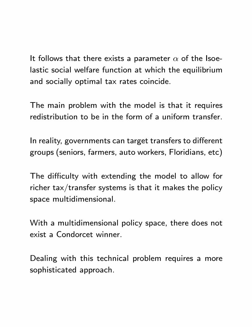
It follows that there exists a parameter of the Isoe-

lastic social welfare function at which the equilibrium

and socially optimal tax rates coincide.

The main problem with the model is that it requires

redistribution to be in the form of a uniform transfer.

In reality, governments can target transfers to different

groups (seniors, farmers, auto workers, Floridians, etc)

The difficulty with extending the model to allow for

richer tax/transfer systems is that it makes the policy

space multidimensional.

With a multidimensional policy space, there does not

exist a Condorcet winner.

Dealing with this technical problem requires a more

sophisticated approach.

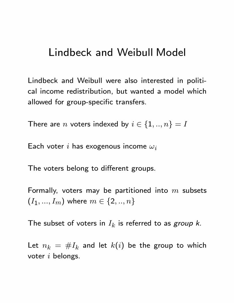
Lindbeck and Weibull Model

Lindbeck and Weibull were also interested in politi-

cal income redistribution, but wanted a model which

allowed for group-specific transfers.

There are voters indexed by ∈ {1 } =

Each voter has exogenous income

The voters belong to different groups.

Formally, voters may be partitioned into subsets

(1 ) where ∈ {2 }

The subset of voters in is referred to as group k.

Let = # and let () be the group to which

voter belongs.

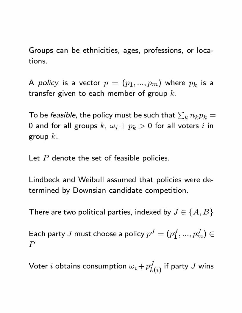
Groups can be ethnicities, ages, professions, or loca-

tions.

A policy is a vector = (1 ) where is a

transfer given to each member of group .

To be feasible, the policy must be such thatP =

0 and for all groups , + 0 for all voters in

group

Let denote the set of feasible policies.

Lindbeck and Weibull assumed that policies were de-

termined by Downsian candidate competition.

There are two political parties, indexed by ∈ {}

Each party must choose a policy = (1 ) ∈

Voter obtains consumption +()

if party wins

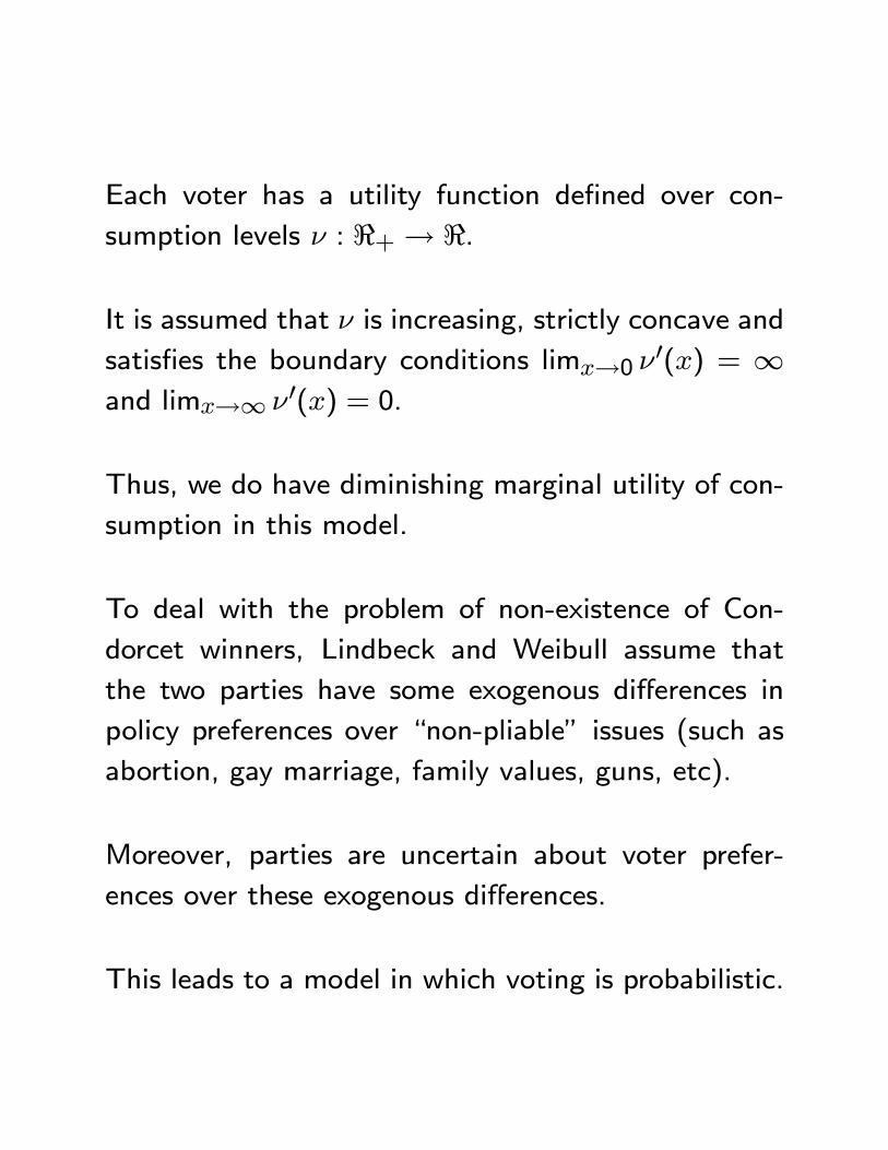
Each voter has a utility function defined over con-

sumption levels : <+→ <.

It is assumed that is increasing, strictly concave and

satisfies the boundary conditions lim→0 0() = ∞and lim→∞ 0() = 0.

Thus, we do have diminishing marginal utility of con-

sumption in this model.

To deal with the problem of non-existence of Con-

dorcet winners, Lindbeck and Weibull assume that

the two parties have some exogenous differences in

policy preferences over “non-pliable” issues (such as

abortion, gay marriage, family values, guns, etc).

Moreover, parties are uncertain about voter prefer-

ences over these exogenous differences.

This leads to a model in which voting is probabilistic.

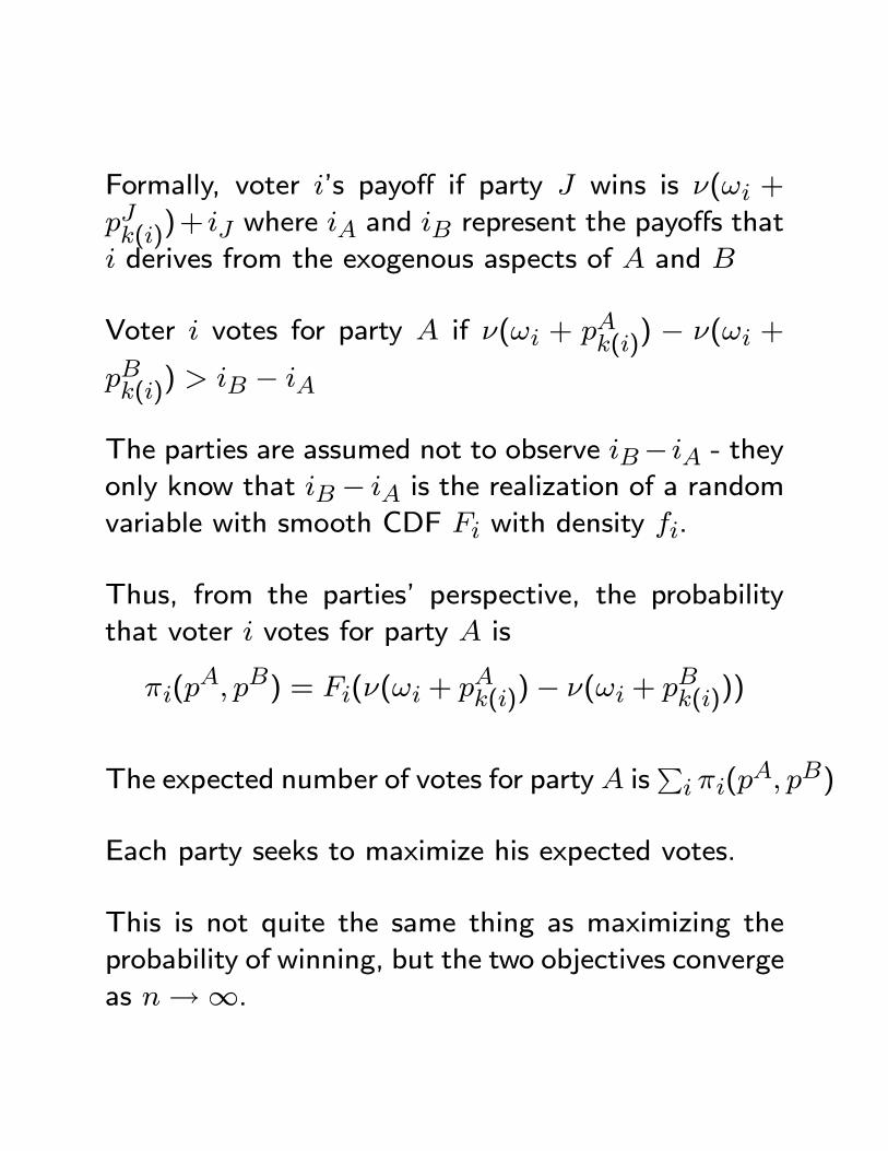
Formally, voter ’s payoff if party wins is ( +

())+ where and represent the payoffs that

derives from the exogenous aspects of and

Voter votes for party if ( + ()) − ( +

()) −

The parties are assumed not to observe − - they

only know that − is the realization of a random

variable with smooth CDF with density .

Thus, from the parties’ perspective, the probability

that voter votes for party is

( ) = (( + ())− ( + ()))

The expected number of votes for party isP (

)

Each party seeks to maximize his expected votes.

This is not quite the same thing as maximizing the

probability of winning, but the two objectives converge

as →∞.

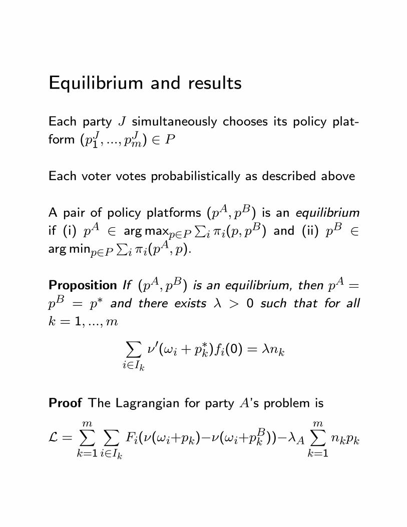
Equilibrium and results

Each party simultaneously chooses its policy plat-

form (1 ) ∈

Each voter votes probabilistically as described above

A pair of policy platforms ( ) is an equilibrium

if (i) ∈ argmax∈P (

) and (ii) ∈argmin∈

P (

).

Proposition If ( ) is an equilibrium, then =

= ∗ and there exists 0 such that for all

= 1 X∈

0( + ∗)(0) =

Proof The Lagrangian for party ’s problem is

L =X=1

X∈

((+)−(+ ))−X=1

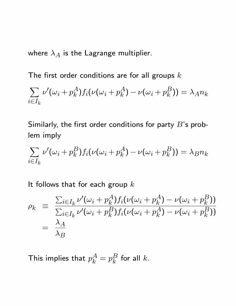
where is the Lagrange multiplier.

The first order conditions are for all groups X∈

0(+ )((+ )− (+ )) =

Similarly, the first order conditions for party ’s prob-

lem implyX∈

0(+ )((+ )− (+ )) =

It follows that for each group

≡P∈

0( + )(( + )− ( + ))P∈

0( + )(( + )− ( + ))

=

This implies that = for all .

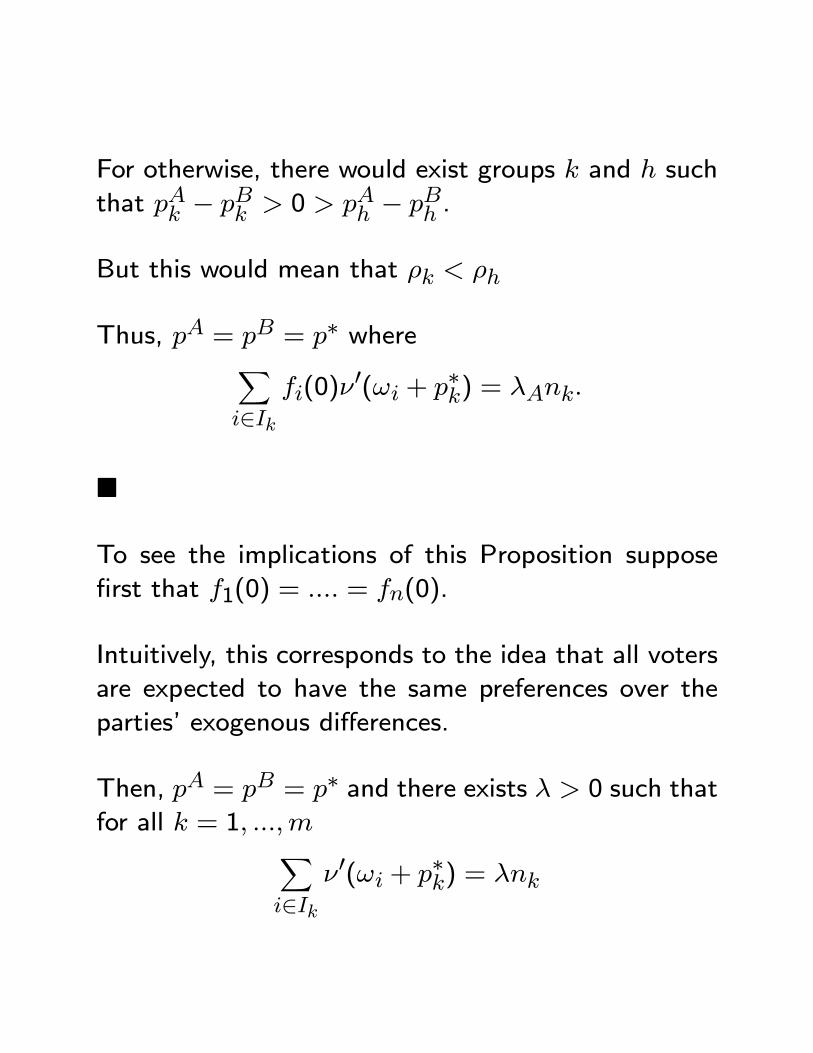
For otherwise, there would exist groups and such

that − 0 − .

But this would mean that

Thus, = = ∗ whereX∈

(0)0( + ∗) =

¥

To see the implications of this Proposition suppose

first that 1(0) = = (0).

Intuitively, this corresponds to the idea that all voters

are expected to have the same preferences over the

parties’ exogenous differences.

Then, = = ∗ and there exists 0 such that

for all = 1 X∈

0( + ∗) =

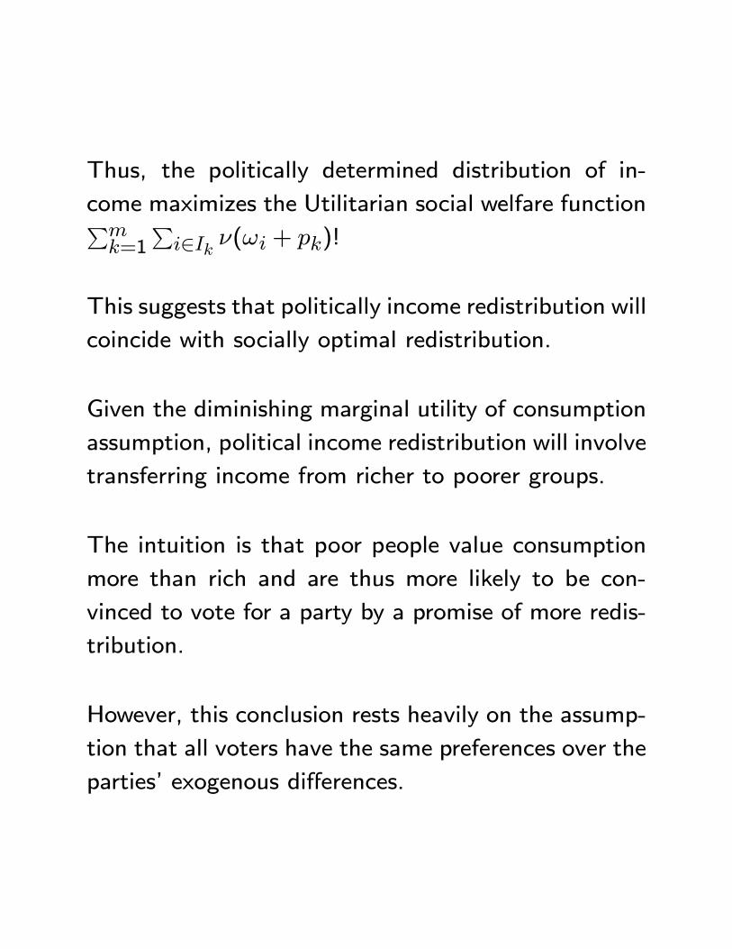
Thus, the politically determined distribution of in-

come maximizes the Utilitarian social welfare functionP=1

P∈ ( + )!

This suggests that politically income redistribution will

coincide with socially optimal redistribution.

Given the diminishing marginal utility of consumption

assumption, political income redistribution will involve

transferring income from richer to poorer groups.

The intuition is that poor people value consumption

more than rich and are thus more likely to be con-

vinced to vote for a party by a promise of more redis-

tribution.

However, this conclusion rests heavily on the assump-

tion that all voters have the same preferences over the

parties’ exogenous differences.

Suppose instead that (i) (0) = (0) for all ∈ and (ii) for all there exists such that

() =

( + ) where is symmetric around 0 and uni-

modal

The parameter can be interpreted as the expected

bias of group in favor of party .

If = 0 group is unbiased; if 0 group is

biased in favor of party and if 0 group is

biased in favor of party

The proposition implies that = = ∗ and thereexists 0 such that for all = 1 P

∈ 0( + ∗)

= ()

The implication of this is that groups who are unbi-

ased get greater transfers or, in other words, political

income redistribution is targeted to groups who are

swing voters.

Obviously, this will not be socially optimal.

Discussion

The Lindbeck-Weibull model has been quite influen-

tial.

Dixit and Londregan (1998) extend the model to allow

the two parties to have different preferences over the

distribution of income.

Swing voters still have an advantage, but now there is

ideologically motivated redistribution as well as tacti-

cal redistribution.

There have been a number of attempts to test the

predictions of the model empirically using location as

the determinant of group identity.

The question is whether states with more swing voters

get more federal money.

There is actually not much evidence for this.

Work on understanding political income redistribution

continues.

III.3 Politics and Efficiency

Will policies emerging from the political process be

Pareto efficient?

This is an interesting and controversial question (see

Wittman (1989) for general discussion).

All the models we have looked at in Part I of the class

suggest that the answer is yes.

In all these models, the implemented policies are Pareto

efficient.

For example, if the implemented policy maximizes the

utility of the median voter then it must be Pareto effi-

cient because any other policy would make the median

voter worse off.

Even if extremist candidates are elected as in the

citizen-candidate model with strategic voting, policies

are still (ex post) Pareto efficient because they max-

imize the utility of those citizens with the extremist

preferences.

Nonetheless, there are a number of types of ineffi-

ciency that have been identified.

We focus primarily on inefficiencies stemming from

reputational concerns and lack of commitment.

III.3.i Reputational inefficiencies

The basic idea is that incumbent politicians want to

preserve good reputations with voters and this some-

times leads them to do inefficient things.

The underlying framework for thinking through these

inefficiencies is the political agency model.

The simplest inefficiency of this type is pandering.

This occurs when politicians choose policies they know

are inefficient just because voters think they are good

policies.

Pandering can arise when politicians have more in-

formation about what the best policies are than do

voters.

I will go through a simple political agency model of

pandering which is simplified version of that used by

Maskin and Tirole in a (2004) paper in American Eco-

nomic Review.

For a related model see Canes-Wrone, Shotts, and

Herron (2001).

A Model of Pandering

There are two time periods, period 1 and period 2.

There are two politicians, an incumbent and a chal-

lenger, and a representative voter.

The incumbent holds office in period 1, but at the

beginning of period 2 faces an election against the

challenger to determine who holds office in period 2.

In each period, the politician who holds office has to

choose policy or policy .

The voter does not know which option is best for him.

In each period, the voter believes that the optimal

policy for him is with probability 12.

Thus, the voter believes that the optimal policy for

him is more likely to be .

The voter’s payoff from the optimal policy is 1 and

from the wrong policy is 0

Importantly, we assume that the voter does not expe-

rience his payoff from the period 1 policy choice until

period 2.

Each politician can be congruent or dissonant.

A congruent politician shares the voter’s policy pref-

erences.

A dissonant politician has the exact opposite prefer-

ences.

When in office, each type of politician (i.e., congruent

or dissonant) gets a policy-related payoff of 1 from

choosing his preferred policy and 0 from the other

policy.

The politician in office is assumed to have more infor-

mation than the voter.

To capture this as simply as possible we assume that

in each period the politician in office is assumed to

know perfectly which option is best for the voter (and

himself).

Each type of politican also gets a non-policy related

payoff when in office.

When not in office, politicians get a payoff of 0.

Politicians discount period 2 payoffs at rate 1.

The voter cannot directly observe politicians’ types.

At the beginning of period 1, he believes the incum-

bent is congruent with probability .

The voter is assumed to observe the incumbent’s pe-

riod 1 policy choice and to update his beliefs about

the incumbent’s type rationally.

Recall that the voter does not observe his payoff from

the period 1 policy choice until period 2.

Game

The game played between the politicians and the voter

is as follows.

In period 1, the incumbent observes what policy is

best for the voter and chooses the policy or .

At the beginning of period 2, the election is held and

the voter chooses whether to re-elect the incumbent

or elect the challenger.

In period 2, the winning politician observes what pol-

icy is best for the voter and chooses the policy or

.

Solving the game

In period 2, whichever politician is holding office will

simply choose his preferred policy - there is no gain

to doing anything else.

Accordingly, at election time, the voter wants to elect

the candidate most likely to be congruent.

Suppose that at the time of the election he believes

the challenger to be congruent with probability and the incumbent to be congruent with probability

0.

Then the voter will re-elect the incumbent if and only

if 0 ≥ .

The key issue is how the voter forms the belief 0.

Intuitively, it should depend on the voter’s initial belief

and also on his period 1 policy choice.

While there are a number of possibilities, we will focus

on the pandering equilibrium.

At the outset, we will make the assumption that =

, so that the voter has the same initial beliefs about

the challenger as he does about the incumbent.

In the pandering equilibrium both types of incumbent

choose policy irrespective of whether it is the best

option for them or the voter.

Then the voter learns nothing about the incumbent’s

type from the period 1 policy choice if he chooses

and thus has no reason to change his prior belief.

What would the voter think if the incumbent were to

choose ?

This is not so clear, because even a congruent politi-

cian could prefer if this were the optimal policy for

the voter.

Nonetheless, since the voter knows that policy is

more likely to be the optimal policy for him, in expec-

tation he knows that dissonant politicians are more

likely to prefer .

Thus, it is natural to assume that the voter would

revise his belief that the incumbent was congruent

downwards if he observed him choosing .

Under this assumption

0 =( if

if

where

Given the assumption that = , it follows that

the voter will re-elect the incumbent if he observes

policy chosen in period 1.

If he observes policy chosen in period 1, the voter

will elect the challenger.

In order for this to be an equilibrium, we need to check

that both types of incumbent will play according to

the proposed equilibrium.

We begin with the Congruent Incumbent.

If the optimal policy is there is nothing to check,

since the congruent incumbent not only prefers but

it also gets him re-elected.

Suppose the optimal policy is .

In this case, if the congruent incumbent chooses his

payoff in period 1 is just , but he gets re-elected and

obtains a payoff in period 2 of 1 + .

His discounted expected payoff from choosing is

therefore

+ [1 + ]

If the congruent incumbent chooses his payoff in

period 1 is 1 + , but he does not get re-elected and

obtains a payoff in period 2 of 0.

His discounted expected payoff from choosing is

therefore

1 +

He will choose if

≥ 1

1 +

We now turn to the Dissonant Incumbent.

If the optimal policy (for the voter) is there is noth-

ing to check, since the dissonant incumbent not only

prefers but it also gets him re-elected.

Suppose the optimal policy (for the voter) is .

In this case, if the dissonant incumbent chooses his

payoff in period 1 is just , but he gets re-elected and

obtains a payoff in period 2 of 1 + .

His discounted expected payoff from choosing is

therefore

+ [1 + ]

If the congruent incumbent chooses his payoff in

period 1 is 1 + , but he does not get re-elected and

obtains a payoff in period 2 of 0.

His discounted expected payoff from choosing is

therefore

1 +

He will choose if

≥ 1

1 +

We have therefore proved the following proposition.

Proposition There exists a pandering equilibrium if

≥ 1(1 + ).

Discussion

To understand the nature of inefficiency here, consider

the case in which the incumbent is congruent and

knows that the optimal policy for the voter is .

Even though both he and the voter prefer policy , he

chooses .

He therefore makes a Pareto inefficient policy choice.

This is a political failure.

The logic of the political failure is that the incumbent

chooses to preserve his reputation with the voter.

Choosing would damage his re-election prospects.

Disguised transfers

Another important example of an inefficiency aris-

ing from reputational concerns is the use of disguised

transfers.

These arise when politicians try to hide the fact that

they are redistributing to a particular group by using

inefficient but sneaky forms of redistribution.

Examples would be a mayor building a convention

center because he wanted to help out his buddies in

the construction industry or legislators ordering a new

fighter plane because they wanted to help out cam-

paign contributors in the defense industry.

Such decisions can be Pareto inefficient if the projects

are so unnecessary that citizens would be better off if

the politicians canceled the project and just gave their

contributors a transfer equal to the profits.

Coate and Morris Model

Coate and Morris (1995) illustrate the use of such in-

efficient disguised transfer mechanisms in a two period

political agency model.

There is a single representative citizen, a special in-

terest (e.g., a construction company), an incumbent

politician, and a challenger.

The incumbent politician is in office at the beginning

of period 1 and faces an election against the challenger

at the beginning of period 2.

In each period, the citizen’s utility is

= − +

where is exogenous income; are taxes; and are

benefits from public projects.

In each period, the special interest’s utility is

= +

where is income derived from public projects and

is a cash transfer.

In period 1, the incumbent chooses a policy ().

∈ <+ is a cash transfer to the special interest and ∈ {} is a discrete public project decision (thinkof this as a construction project).

= means the project is undertaken, =

means it is not.

In period 2, the winner of the election just chooses a

policy .

The public project provides income to the special

interest and has a tax cost to the citizen .

The benefits of the project to the citizen are ∈{} where 0 .

Let = Pr{ = } and assume that ∈ {0 1}where 0 0 1 1.

The expected net benefits of the project to the citizen

given are

∆() = + (1− ) −

Assumption 1 (i) ∆(1) 0 and (ii) ∆(0) −

Thus, when = 1, the project is an expected Pareto

improvement.

When = 0, the project is an inefficient way of

redistributing to the special interest.

Assume that, as far as the citizen knows, Pr{ =

1} = .

Each politican can be either good or bad.

Each type receives a per-period payoff 0 when not in

office.

When in office, a good politician receives a payoff

( − ) where 0(·) 0 and (0) 0

A bad politician receives (− ) where 0 and 0 and (0 0) 0.

Thus bad politicians wish to help the special interest.

Assumption 2 (∆(0) ) (0 0)

This says that bad politicians prefer introducing the

inefficient project than doing nothing.

The citizen faces two types of uncertainty:

(i) Policy uncertainty - he does not observe the real-

ization of whereas the incumbent politician does.

Note that he cannot infer ex post since even a good

project may fail.

(ii) Politician uncertainty - he does not observe the

type of the incumbent or the challenger.

Let be his prior that the incumbent is good and let

be his prior that the challenger is good.

is a given, while is realized at the time of the

election - ex ante, it is draw from the CDF ()

Game and equilibrium

The game played between the incumbent, challenger

and voter has the following timing.

1. The quality of project ∈ {0 1} is chosen - thisis observed only by the incumbent.

2. The incumbent chooses () ∈ <+ × {} -this is observed by the citizen.

3. If = , the benefits from the project ∈{} are realized and this is observed by thecitizen.

4. The reputation of the challenger is determined.

5. Knowing and incumbent’s first period record

() the citizen decides whether to re-elect the

incumbent.

6. The winner of the election chooses second period

.

A strategy for the incumbent consists of a first pe-

riod policy choice conditional on his type and and a

second period transfer conditional on his type.

A strategy for the challenger consists of a second pe-

riod transfer conditional on his type.

A strategy for the citizen is a rule specify the proba-

bility that he will re-elect the incumbent conditional

on () and .

We also need to specify the citizen’s beliefs concerning

the probability that the incumbent is good which we

denote ().

An equilibrium consists of strategies for all the players

that are optimal and beliefs for the citizen which are

consistent with the strategy of the incumbent of this

game.

Main result

Proposition Under appropriate assumptions, there ex-

ists b such that if b, in any equilibrium a bad

incumbent always chooses (0 ) and a good incum-

bent chooses (0 ) when = 0 and (0 ) when

= 1.

Thus, when = 0 the bad incumbent redistributes

inefficiently.

The logic is that the reputational penalty for choosing

the project is less severe than that for choosing cash

transfers.

This is because the good incumbent chooses the project

when it is a good idea and the voter cannot observe

whether it is a good idea.

The project is therefore a disguised transfer.

Note that for a public project to be a disguised transfer

it must have four key features.

(i) It benefits a special interest.

(ii) It may or may not benefit the rest of society.

(iii) Citizens have less information on the project’s

expected benefits than do politicians.

(iv) Citizens cannot infer the project quality ex post.

Many public projects have these features.

Coate and Morris also show that for the argument to

make sense, voters must be uncertain of the incum-

bent’s desire to redistribute to the special interest.

If all incumbents are bad, then there is nothing to hide

and voters penalize inefficient redistribution.

In essence, the use of disguised transfers arises from

the desire of incumbents to avoid losing their reputa-

tions as being on the side of taxpayers (as opposed to

special interests).

Discussion

The above examples illustrate how reputational con-

cerns can lead to inefficiencies.

There are by now many papers with a similar theme.

Two other nice examples are Groseclose and McCarty

(2001) and Majumdar and Mukand (2004).

III.3.ii Commitment problems

The literature has identified a number of reasons why

public policy decisions with dynamic consequences (such

as budget deficits or public investments) may be inef-

ficient.

The fundamental factor underlying these inefficiencies

is lack of commitment - there is no mechanism by

which future leaders can commit to current policy-

makers what their policy choices will be.

We will illustrate these problems with two examples.

The first example illustrates why a reform with short

run costs but long run benefits is not undertaken.

The second example shows why debt levels can be too

high.

Reform example

This example is based on Besley and Coate (1998).

Consider a society of citizens divided equally into

two groups, and .

Suppose that there are two time periods, period 1 and

period 2.

In period 1, the society can undertake a reform.

The reform imposes costs on members of group in

period 1, but benefits all citizens in period 2.

Good examples might be the removal of a trade barrier

protecting group or a subsidy benefiting group .

The per-citizen cost to members of group in period

1 is and the per-citizen benefit to all citizens in

period 2 is .

Let denote citizens’ discount rate, and assume that

the discounted aggregate benefits of the reform ex-

ceed the aggregate costs.

Formally, the condition is

2

Also assume that that the reform does not directly

benefit members of group

Formally, this condition is that

However, assume that the government can levy a tax

on the period 2 benefits of the reform and compensate

members of group by redistributing the revenues to

them.

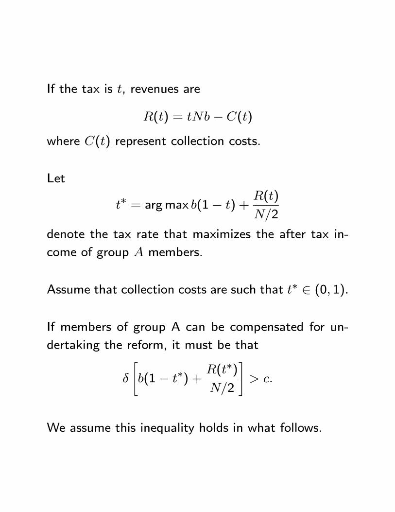
If the tax is , revenues are

() = − ()

where () represent collection costs.

Let

∗ = argmax (1− ) +()

2

denote the tax rate that maximizes the after tax in-

come of group members.

Assume that collection costs are such that ∗ ∈ (0 1).

If members of group A can be compensated for un-

dertaking the reform, it must be that

"(1− ∗) + (∗)

2

#

We assume this inequality holds in what follows.

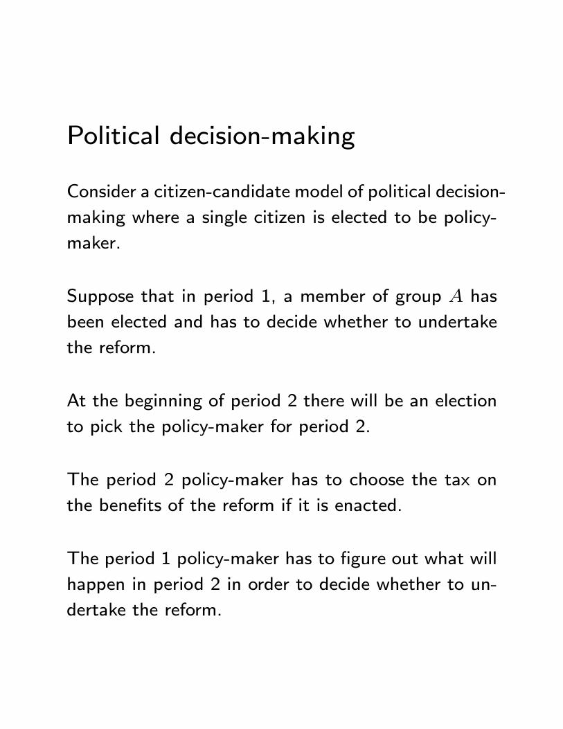
Political decision-making

Consider a citizen-candidate model of political decision-

making where a single citizen is elected to be policy-

maker.

Suppose that in period 1, a member of group has

been elected and has to decide whether to undertake

the reform.

At the beginning of period 2 there will be an election

to pick the policy-maker for period 2.

The period 2 policy-maker has to choose the tax on

the benefits of the reform if it is enacted.

The period 1 policy-maker has to figure out what will

happen in period 2 in order to decide whether to un-

dertake the reform.

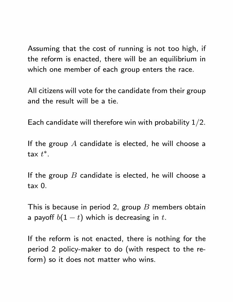
Assuming that the cost of running is not too high, if

the reform is enacted, there will be an equilibrium in

which one member of each group enters the race.

All citizens will vote for the candidate from their group

and the result will be a tie.

Each candidate will therefore win with probability 12.

If the group candidate is elected, he will choose a

tax ∗.

If the group candidate is elected, he will choose a

tax 0.

This is because in period 2, group members obtain

a payoff (1− ) which is decreasing in .

If the reform is not enacted, there is nothing for the

period 2 policy-maker to do (with respect to the re-

form) so it does not matter who wins.

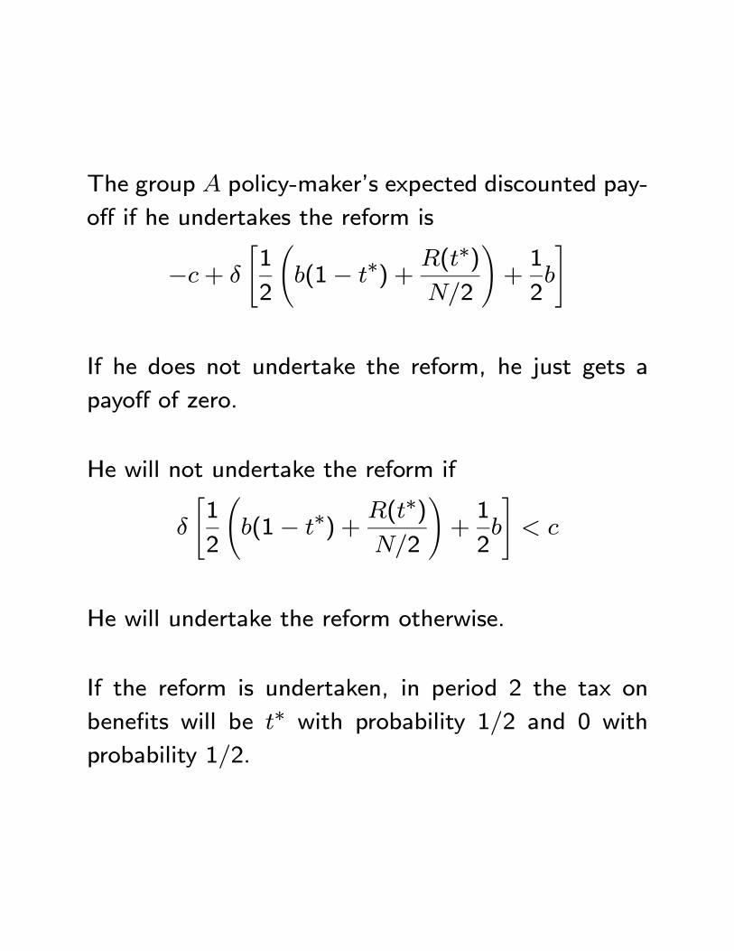
The group policy-maker’s expected discounted pay-

off if he undertakes the reform is

−+

"1

2

Ã(1− ∗) + (∗)

2

!+1

2

#

If he does not undertake the reform, he just gets a

payoff of zero.

He will not undertake the reform if

"1

2

Ã(1− ∗) + (∗)

2

!+1

2

#

He will undertake the reform otherwise.

If the reform is undertaken, in period 2 the tax on

benefits will be ∗ with probability 12 and 0 withprobability 12.

Political failure

If the reform is not undertaken, the politically deter-

mined policy choice will be Pareto inefficient.

The policy choice of no reform is Pareto dominated

by the policy choice that involves the reform being

undertaken in period 1 and, in period 2, the benefits

being taxed at rate ∗ and the revenues given to group members.

Political decision-making in this example therefore gives

rise to political failure.

The intuition underlying the political failure is as fol-

lows.

In order to make the reform Pareto improving, Group

A members must be compensated for incurring the

short run costs of the reform from the future benefits.

However, Group A members realize that when com-

pensation can be paid they may no longer hold power.

They understand that if Group B members control

policy they will not receive compensation.

This is because by then the reform has been imple-

mented and Group B members have no incentive to

compensate Group A.

Because of this concern, Group A members do not

introduce the reform in the first place.

In order for the story to hold together, it must be that

the group who currently holds power must anticipate

losing that power in the future.

To resolve this inefficiency, Group B needs to commit

to Group A that it will compensate them when the

benefits of the reform are realized if it holds power.

Unfortunately, such future commitments are difficult

in the political process.

This is because the future decision-makers are not

even selected yet.

Debt example

This example is based on Alesina and Tabellini (1990).

Consider a legislature which consists of representatives

from two Parties and .

There are two time periods, period 1 and period 2.

The legislature uses revenues to finance projects.

There are two types of projects: projects and

projects.

Let and denote spending on projects and

projects in period ∈ {1 2}.

party representatives only care about spending on

projects and party representatives only care about

spending on projects.

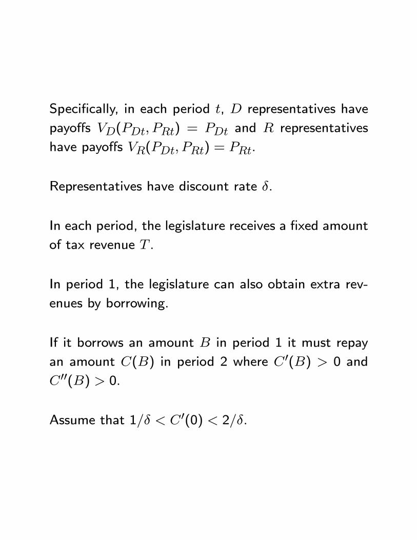
Specifically, in each period , representatives have

payoffs ( ) = and representatives

have payoffs ( ) = .

Representatives have discount rate .

In each period, the legislature receives a fixed amount

of tax revenue .

In period 1, the legislature can also obtain extra rev-

enues by borrowing.

If it borrows an amount in period 1 it must repay

an amount () in period 2 where 0() 0 and

00() 0.

Assume that 1 0(0) 2.

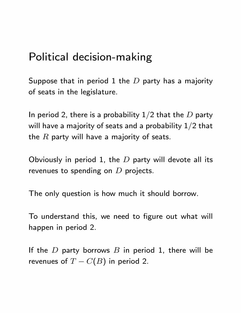
Political decision-making

Suppose that in period 1 the party has a majority

of seats in the legislature.

In period 2, there is a probability 12 that the party

will have a majority of seats and a probability 12 that

the party will have a majority of seats.

Obviously in period 1, the party will devote all its

revenues to spending on projects.

The only question is how much it should borrow.

To understand this, we need to figure out what will

happen in period 2.

If the party borrows in period 1, there will be

revenues of − () in period 2.

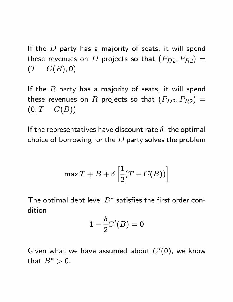
If the party has a majority of seats, it will spend

these revenues on projects so that (2 2) =

( − () 0)

If the party has a majority of seats, it will spend

these revenues on projects so that (2 2) =

(0 − ())

If the representatives have discount rate , the optimal

choice of borrowing for the party solves the problem

max + +

∙1

2( − ())

¸

The optimal debt level ∗ satisfies the first order con-dition

1−

20() = 0

Given what we have assumed about 0(0), we knowthat ∗ 0.

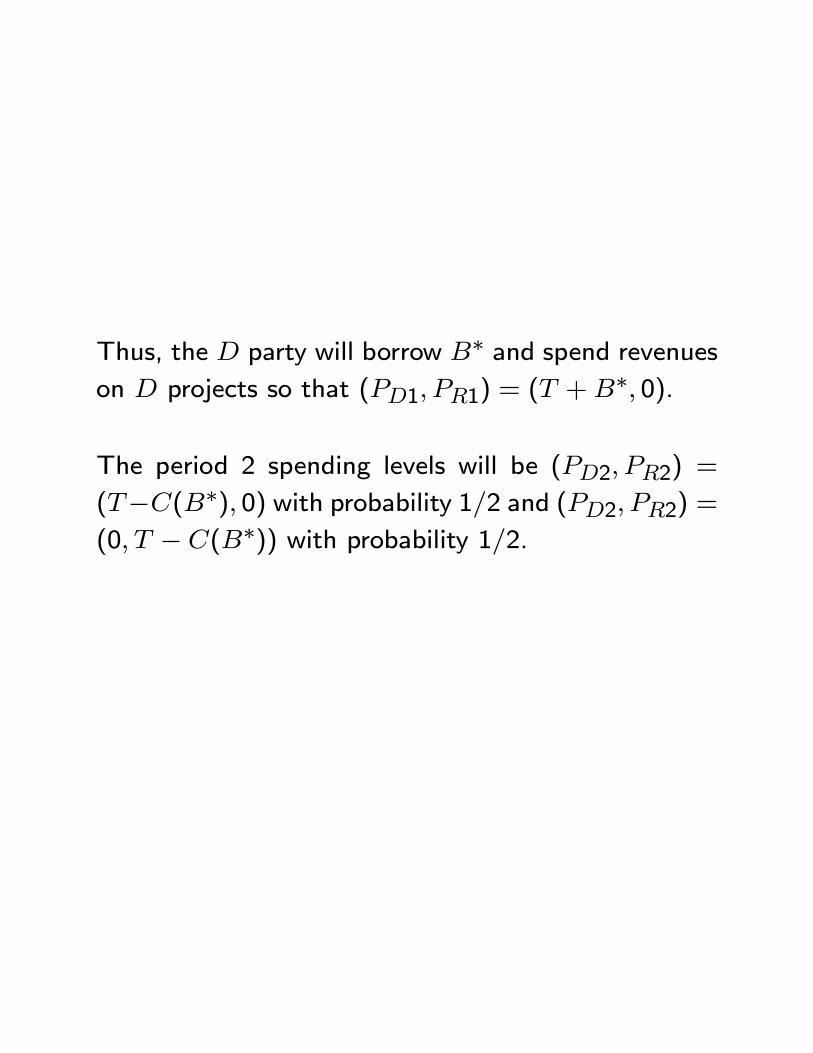
Thus, the party will borrow ∗ and spend revenueson projects so that (1 1) = ( +∗ 0).

The period 2 spending levels will be (2 2) =

(−(∗) 0) with probability 1/2 and (2 2) =(0 − (∗)) with probability 1/2.

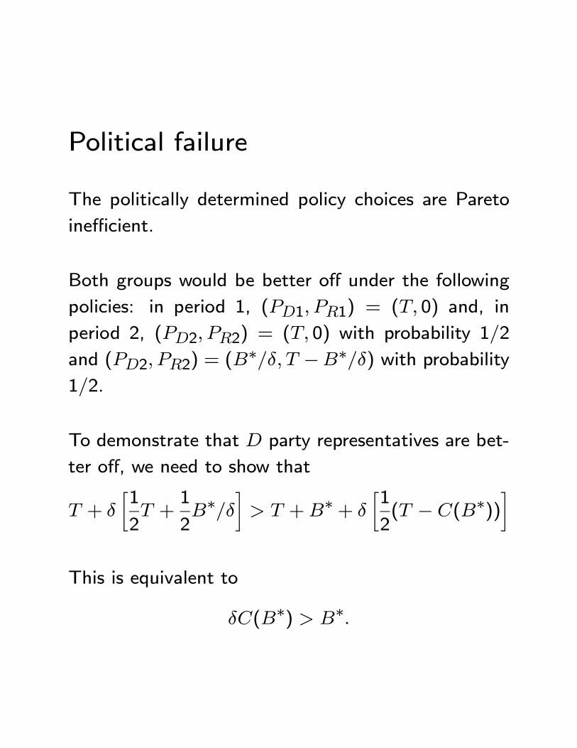
Political failure

The politically determined policy choices are Pareto

inefficient.

Both groups would be better off under the following

policies: in period 1, (1 1) = ( 0) and, in

period 2, (2 2) = ( 0) with probability 1/2

and (2 2) = (∗ −∗) with probability

1/2.

To demonstrate that party representatives are bet-

ter off, we need to show that

+

∙1

2 +

1

2∗

¸ +∗+

∙1

2( − (∗))

¸

This is equivalent to

(∗) ∗

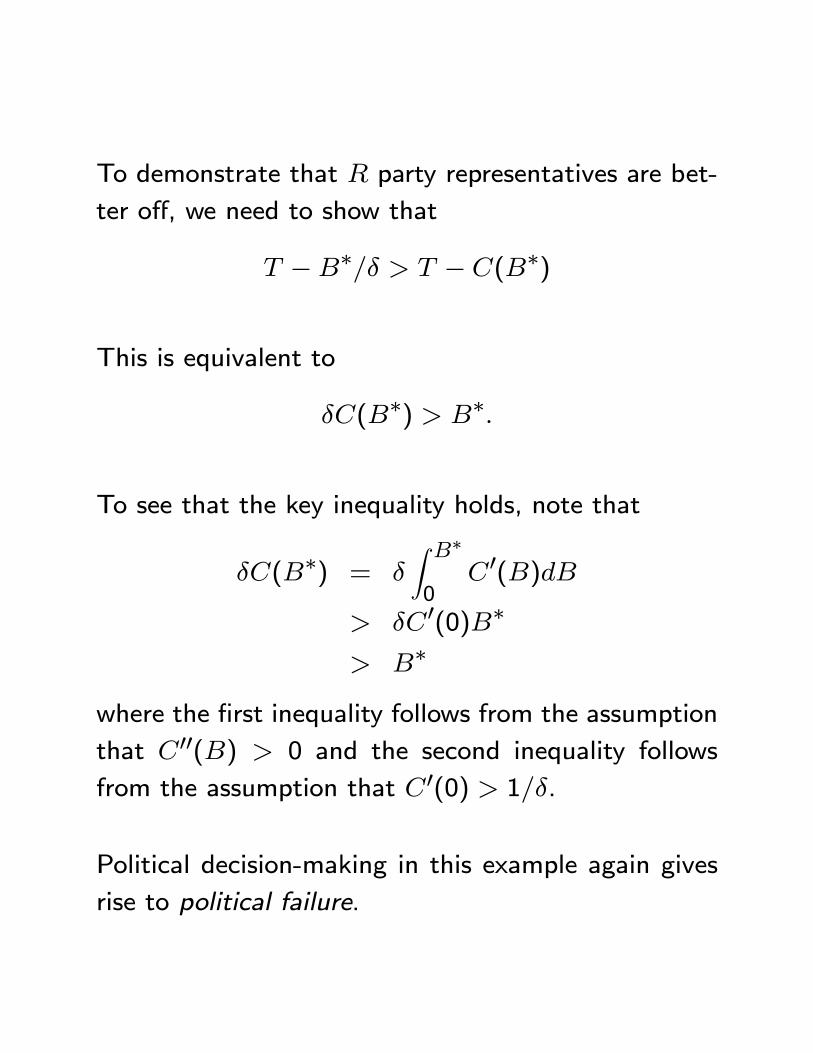
To demonstrate that party representatives are bet-

ter off, we need to show that

−∗ − (∗)

This is equivalent to

(∗) ∗

To see that the key inequality holds, note that

(∗) =

Z ∗

00()

0(0)∗

∗

where the first inequality follows from the assumption

that 00() 0 and the second inequality follows

from the assumption that 0(0) 1.

Political decision-making in this example again gives

rise to political failure.

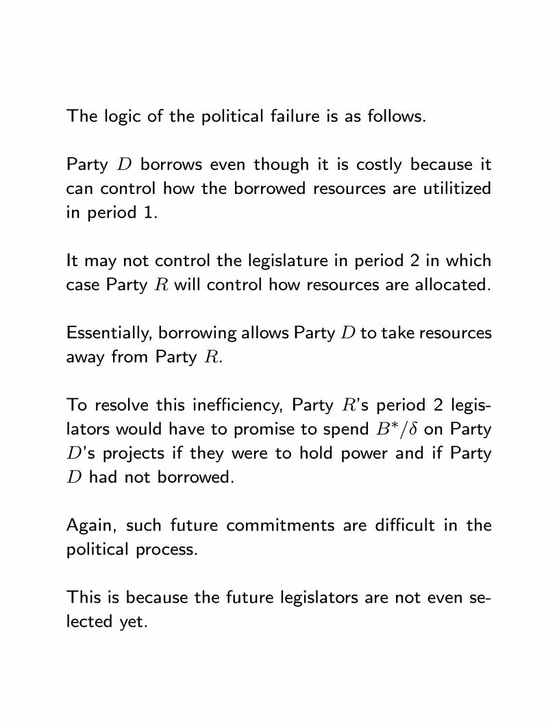
The logic of the political failure is as follows.

Party borrows even though it is costly because it

can control how the borrowed resources are utilitized

in period 1.

It may not control the legislature in period 2 in which

case Party will control how resources are allocated.

Essentially, borrowing allows Party to take resources

away from Party .

To resolve this inefficiency, Party ’s period 2 legis-

lators would have to promise to spend ∗ on Party’s projects if they were to hold power and if Party

had not borrowed.

Again, such future commitments are difficult in the

political process.

This is because the future legislators are not even se-

lected yet.

Discussion

There are many other papers exploring political fail-

ures arising from lack of commitment in a variety of

dynamic contexts.

See Acemoglu (2003), Acemoglu and Robinson (2001),

Azzimonti (2011), Battaglini and Coate (2008), and

Hassler et al (2003).

III.3.iii Political risk

So far, our discussion of inefficiency has focused on

ex post Pareto inefficiency; i.e., can the policy that is

actually chosen be Pareto dominated?

The literature has also looked at ex ante Pareto inef-

ficiency which takes into account the costs of any risk

that arises in political outcomes.

For example, in the model of candidate competition

with policy-motivated candidates or the citizen can-

didate model, risk arises because candidates choose

different policies and it is uncertain which candidate

will win.

If individuals are risk averse, this uncertainty will be

costly.

On the other hand, if there is aggregate uncertainty

in citizens’ preferences, the fact that candidates have

different positions provides an option value to society.

This raises the question of whether candidates will be

optimally differentiated.

On this issue see Bernhardt, Duggan, and Squintani

(2009).

III.4 Implications for the Role ofGovernment

There is no good reason to expect policies emerging

from the political process to produce policies that are

socially optimal according to commonly used social

welfare functions.

The issue of the Pareto efficiency of politically deter-

mined policies is a little more subtle, but we have iden-

tified solid reasons why even this will not be achieved.

In terms of what all this means, there are three points

to note.

Point 1

The first point to note is that the prescriptions of

normative theories of government can not simply be

interpreted as positive predictions.

We need to study politics if we want to explain policy

choices.

This is comforting, but not particularly surprising.

Point 2

The second point to note is that we need to rethink

our standard justifications for government interven-

tion.

To illustrate, consider the standard analysis of inter-

vention to deal with an externality.

Figure 1 depicts the textbook analysis of a polluting

industry.

The good is produced at constant cost and the mar-

ket equilibrium is units.

The textbook approach recommends intervention us-

ing a corrective tax on the grounds that aggregate

welfare would be higher if the tax were set at ∗, theaggregate utility maximizing level.

However, as we have argued, there is no reason to

expect the political process to set the tax at the ag-

gregate utility maximizing level.

The political economist would argue that intervention

should be recommended only if aggregate surplus at

the politically determined level of the tax is higher

than at the market equilibrium.

There is no guarantee that this would be the case.

Suppose, for example, that a pro-environment lobby

group would pressure policy makers to set a tax equal

to b.Then the intervention would actually reduce aggregate

utility.

Acccordingly, the economic policy analyst should an-

ticipate the politically determined level and take this

into account.

This leads to more conservative policy advice because

political determination of the new policy is a con-

straint on policy choices that makes intervention less

attractive.

Point 3

Taking into account political distortions can also jus-

tify imposing fiscal restraints on government.

Fiscal restraints include limitations on the types and

levels of taxes, balanced budget requirements, spend-

ing limits, etc.

The idea is that such restraints can be written into a

society’s constitution and are therefore hard for politi-

cians to overcome.

In the debt example, for example, it would be good

idea to require the government to run a balanced bud-

get.

This would restore efficiency.

We will come back to look at fiscal restraints in more

detail later in the class.

IV Contemporary Political Issues

We now apply some of the tools we have learned to

think about some current political issues.

We begin with districting.

IV.1 Districting

Districting refers to the process by which political dis-

tricts are redrawn to reflect population changes.

For example, suppose there are seats in the legis-

lature and that legislators are elected by distinct

political districts.

Each district is required to have approximately the

same population.

Then if the population changes, the districts have to

be withdrawn: districting refers to that process.

For U.S. house elections, districting is done at the

state level.

The relative size of a state determines the size of its

congressional delegation.

The state then divides up the population into political

districts that will elect these representatives.

Districting must also be done for the election of state

legislatures, county legislatures and city councils.

Indeed, districting is an essential part of any political

system with geographic based (as opposed to at large)

representation.

Districting in the U.S. is typically done on a ten year

cycle following the dicennial census.

In the U.S., districting is often a highly controversial

process.

There are two main issues: partisan districting and

racial districting.

With partisan districting, districters design districts

with an eye towards increasing the representation of

legislators from a particular party or ideology.

This process is also known as gerrymandering after

Governor Elbridge Gerry of MA who designed a salamander-

shaped electoral district in the nineteenth century.

To illustrate, consider a legislature with 10 seats and

two parties Democrats and Republicans.

Suppose that 50% of the population are Democrats

and 50% are Republicans.

Then, while the aggregate vote share for the De-

mocrats will be 50%, they can get anywhere between

1 and 9 seats depending on how the districts are cre-

ated.

For example, they can get 9 seats by creating 9 dis-

tricts that are 51% Democrat.

Relatedly, districting can also be designed to protect

incumbents.

Thus, the idea is that districters conspire to design

districts to maximize the chances that incumbents are

reelected.

For example, by adding more Republicans to the dis-

tricts of Republican incumbents.

This is called a bipartisan gerrymander.

With racial districting, redistricters design districts

with an eye towards minimizing the political influence

of a particular ethnic group - typically, African Amer-

icans.

The topic of districting has attracted a great deal of

attention from political scientists and political econo-

mists.

It is a subject that is historically rich, the underly-

ing theoretical issues are interesting, and the topic is

practical and policy relevant.

We will focus on the literature on partisan districting.

We discuss three topics: seat-vote curves; optimal

partisan gerrymandering; and socially optimal district-

ing.

IV.1.i Seat-vote curves

The standard way of thinking about districting plans

is in terms of the seat-vote curves they generate.

The seat-vote curve gives the relationship between one

party’s seats in the legislature and its aggregate vote.

Formally, it is represented by a function ( ) where

∈ [0 1] is the aggregate fraction of votes receivedby (say) the Democrats and ∈ [0 1] is the fractionof seats in the legislature that they hold.

For example, in a PR system, ( ) = and in a

winner take all system

( ) =

(1 if 12

0 if 12

It should be clear intuitively that different districtings

will give rise to very different seat-vote curves.

In our earlier example with a 10 seat legislature, was

05 while (05) could be any number in {01 09}.

Key properties of seat-vote curves are partisan bias

and responsiveness.

A seat vote curve exhibits partisan symmetry if ( ) =

1− (1− ) for all .

Intuitively, what this means is that the Democrat seat

share when it has a particular fraction of the votes

is the same as the Republican seat share when it has

that same fraction of votes.

A seat-vote curve exhibits partisan bias if it deviates

from partisan symmetry in a systematic way.

The simplest way of measuring this bias is just to look

at the difference (12)− 12.

If this difference is postive, the bias favors Democrats

and if it is negative, the bias favors Republicans.

The responsiveness of a seat-vote curve is measured

by the proportionate change in seat share following an

increase in vote share; that is,

( +∆ )− ( )

∆

If the seat-vote curve is differentiable, then its respon-

siveness at is measured by the derivative 0( ).

In the case of a linear seat-vote curve, partisan bias

and responsiveness can be defined unambiguously.

The linear seat-vote curve can be written as

( ) =1

2+ + ( − 1

2)

where the parameter measures partisan bias and

measures responsiveness.

The political science literature has devised ever more

sophisticated methods for estimating seat-vote curves.

Sample references are Tufte (1973), King (1989), and

Gelman and King (1994).

A standard exercise is to estimate the seat-vote curves

for a state legislature associated with particular dis-

tricting plans (recall that districting is changed every

10 years).

The analyst then studies how partisan bias and re-

sponsiveness change as the districting plan changes.

It is also common to study how the changes in bias

and responsiveness depend on the process by which

districting is done at the state level.

Some states have partisan districting processes; others

bipartisan districting processes; and still others non-

partisan districting processes.

A standard finding is that partisan districting increases

partisan bias and responsiveness; bipartisan districting

reduces bias and responsiveness; non-partisan district-

ing increases responsiveness and has no effect on bias.

IV.1.ii Optimal partisan gerrymander-ing

How should a party that controls the districting process

choose a districting plan to maximize the probability

of controlling the legislature?

This is a classic question in theoretical political sci-

ence.

Lets work through a simple model to illustrate the

main principles underlying an optimal partisan gerry-

mander.

The model is taken from Coate and Knight (2007).

A simple districting model

Consider a community in which there are three types

of voters: Democrats, Independents, and Republicans.

Democrats and Republicans have ideologies 0 and 1,

respectively.

Independents have ideologies that are uniformly dis-

tributed on the interval [− + ] where 0

and is the realization of a random variable uni-

formly distributed on [12 − 12 + ], where ∈(0 ) and + 12.

This is similar to the set up we used in Section I.2.ii -

is the ideology of the median Independent voter.

The fractions of voters who are Democrats, Indepen-

dents, and Republicans are , , and .

Policy choices are made by a 3-seat legislature (we

assume 3 just for tractability).

The policy outcomes chosen by the legislature depend

upon the ideology of the median legislator.

Voters have quadratic preferences so that if the me-

dian legislator has ideology 0, a voter with ideology obtains a payoff given by −(− 0)2.

There are two political parties: the Democrats and

Republicans.

The Democrat Party consists of Democrats and the

Republican Party consists of Republicans.

Legislators are all affiliated with one or the other party.

To select legislators, the state is divided into 3 equally

sized districts indexed by ∈ {1 2 3}

Each district then elects a legislator.

Candidates are put forward by the two political parties.

The Democrat Party puts up Democrats and the Re-

publican Party puts up Republicans.

The citizen-candidate model applies so legislators just

follow their true ideologies when elected - Democrats

0 and Republicans 1.

Elections are held simultaneously in each of the 3 dis-

tricts and the candidate with the most votes wins.

In each district, voters vote sincerely for the represen-

tative whose ideology is closest to their own.

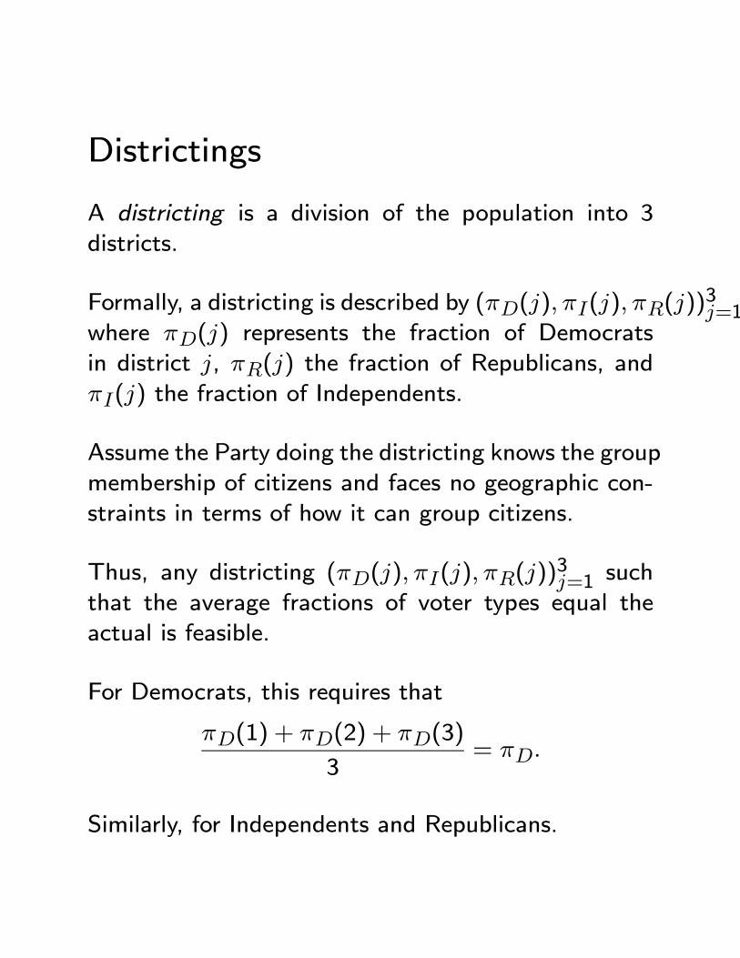
Districtings

A districting is a division of the population into 3

districts.

Formally, a districting is described by (() () ())3=1

where () represents the fraction of Democrats

in district , () the fraction of Republicans, and

() the fraction of Independents.

Assume the Party doing the districting knows the group

membership of citizens and faces no geographic con-

straints in terms of how it can group citizens.

Thus, any districting (() () ())3=1 such

that the average fractions of voter types equal the

actual is feasible.

For Democrats, this requires that

(1) + (2) + (3)

3=

Similarly, for Independents and Republicans.

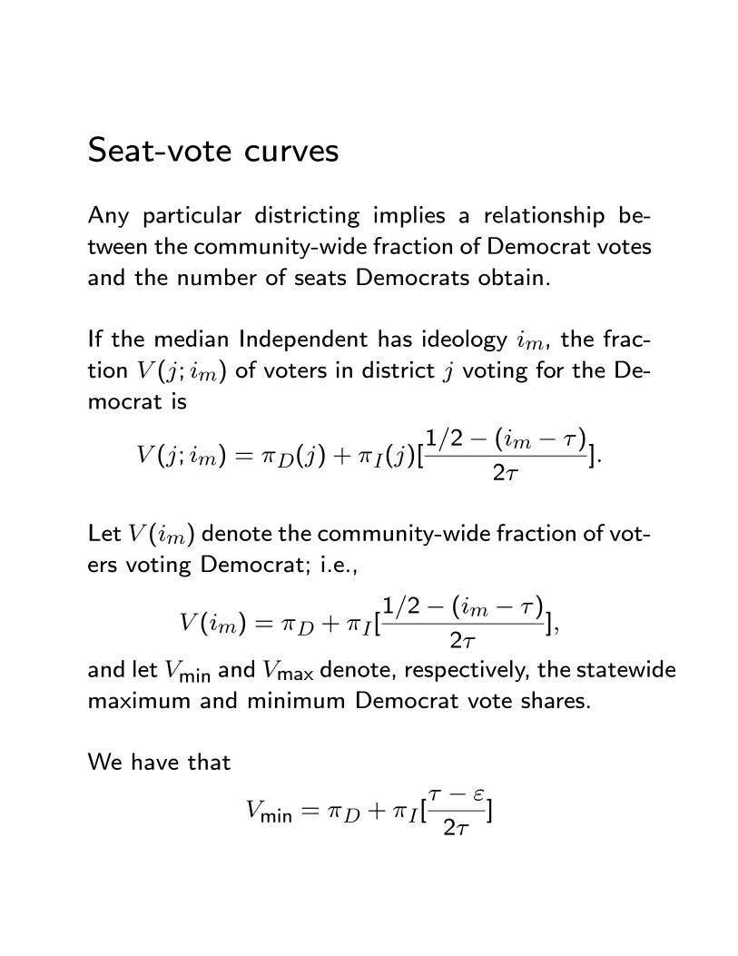
Seat-vote curves

Any particular districting implies a relationship be-

tween the community-wide fraction of Democrat votes

and the number of seats Democrats obtain.

If the median Independent has ideology , the frac-

tion (; ) of voters in district voting for the De-

mocrat is

(; ) = () + ()[12− ( − )

2]

Let () denote the community-wide fraction of vot-

ers voting Democrat; i.e.,

() = + [12− ( − )

2]

and let min and max denote, respectively, the statewide

maximum and minimum Democrat vote shares.

We have that

min = + [ −

2]

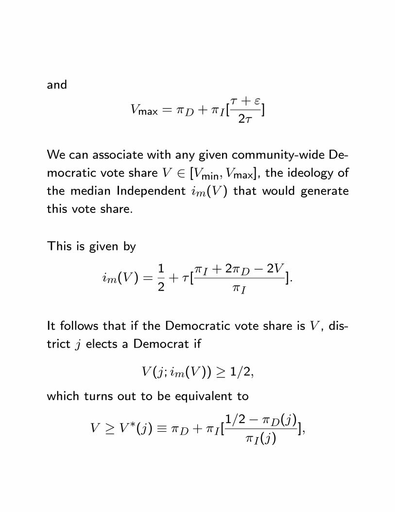
and

max = + [ +

2]

We can associate with any given community-wide De-

mocratic vote share ∈ [min max], the ideology ofthe median Independent ( ) that would generate

this vote share.

This is given by

( ) =1

2+ [

+ 2 − 2

].

It follows that if the Democratic vote share is , dis-

trict elects a Democrat if

(; ( )) ≥ 12which turns out to be equivalent to

≥ ∗() ≡ + [12− ()

()]

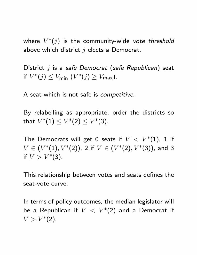
where ∗() is the community-wide vote thresholdabove which district elects a Democrat.

District is a safe Democrat (safe Republican) seat

if ∗() ≤ min (∗() ≥ max).

A seat which is not safe is competitive.

By relabelling as appropriate, order the districts so

that ∗(1) ≤ ∗(2) ≤ ∗(3).

The Democrats will get 0 seats if ∗(1), 1 if ∈ ( ∗(1) ∗(2)), 2 if ∈ ( ∗(2) ∗(3)), and 3if ∗(3)

This relationship between votes and seats defines the

seat-vote curve.

In terms of policy outcomes, the median legislator will

be a Republican if ∗(2) and a Democrat if ∗(2).

Partisan gerrymandering

Suppose that the Democrats control the districting

authority and want to come up with a districting plan

that maximizes the probability that the Democrats

have a majority of seats.

Clearly, they needs to choose a districting that maxi-

mizes the probability that ∗(2).

This involves making ∗(2) as small as possible.

To make things interesting assume that 13

The Democrats do not care who wins district 3.

Thus, it is obvious that the solution will involve pack-

ing district 3 with Republicans; i.e., ((3) (3) (3)) =

(0 0 1).

For districts 1 and 2, ((1) (1)) and ((2) (2))

solve the problem

min ∗(2) ∗(1) ≤ ∗(2)(1)+(2)

3=

(1)+(2)3

=

This looks complicated but it is not really.

Since there is no gain to making District 1 any easier

to win than District 2, it is clear that

∗(1) = ∗(2)

This goal can be achieved by setting ((1) (1))

equal to ((2) (2)).

But then from the constraints we get that (1) =

(2) =32 and that (1) = (2) =

32.

It follows that

((1) (1) (1)) = ((2) (2) (2))

= (3

2

3

2

3

2 −

1

2)

Notice that the Republicans who cannot be fit into

District 3 are spread evenly over the other districts.

This strategy for dealing with the opposition voters is

sometimes referred to as cracking and packing.

You pack a minority of districts with the opposition

and then spread the remainder smoothly over the ma-

jority districts.

Notice that under the optimal districting plan

∗(2) = + [12− (2)

(2)]

=1

3

It follows that the Democrats will hold a majority of

seats with probability 1 if min 13

Using the expression for min, this condition amounts

to

+ [ −

2] 13

If this condition is not satisfied, the probability that

the Democrats will hold a majority of seats is the prob-

ability that ≥ 13

This probability is given by

max − 13max − min

= + [

+2]− 13

³

´

Note that the seat-vote curve generated by this dis-

tricting plan displays extreme partisan bias in favor

of Democrats since they get more than 1/2 the seats

with only 1/3 of the votes.

For more on optimal partisan gerrymandering see Fried-

man and Holden (2008).

See also Gul and Pesendorfer (2010) for an interesting

analysis of what happens when the two parties control

different states and choose their districting strategies

in competitive fashion.

IV.1.iii Socially optimal districting

The previous exercise explores how a party should

choose a districting plan to maximize political advan-

tage.

A more public-spirited question is this: how should a

districting authority that controls the districting process

choose a districting plan?

The way this is usually approached is in terms of the

shapes of the districts: for example, a good districting

plan should have appropriately “compact” districts.

There are alternative ways of measuring the compact-

ness of political districts - see, for example, Fryer and

Holden (in press).

A more economic way to think about it is to ask what

districting plan will maximize social welfare as mea-

sured by a social welfare function?

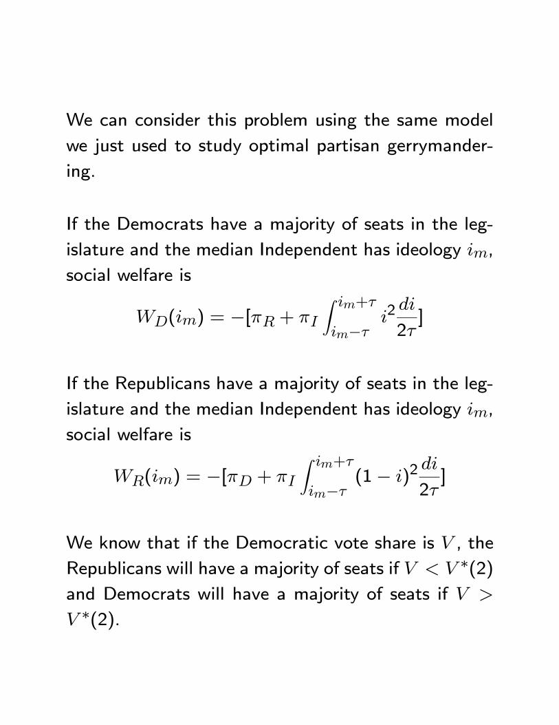
We can consider this problem using the same model

we just used to study optimal partisan gerrymander-

ing.

If the Democrats have a majority of seats in the leg-

islature and the median Independent has ideology ,

social welfare is

() = −[ +

Z +

−2

2]

If the Republicans have a majority of seats in the leg-

islature and the median Independent has ideology ,

social welfare is

() = −[ +

Z +

−(1− )2

2]

We know that if the Democratic vote share is , the

Republicans will have a majority of seats if ∗(2)and Democrats will have a majority of seats if

∗(2).

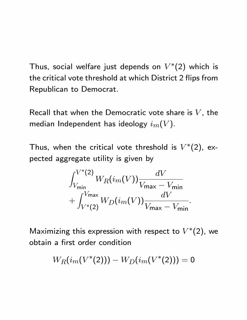
Thus, social welfare just depends on ∗(2) which isthe critical vote threshold at which District 2 flips from

Republican to Democrat.

Recall that when the Democratic vote share is , the

median Independent has ideology ( ).

Thus, when the critical vote threshold is ∗(2), ex-pected aggregate utility is given byZ ∗(2)

min(( ))

max − min

+

Z max

∗(2)(( ))

max − min

Maximizing this expression with respect to ∗(2), weobtain a first order condition

((∗(2)))−((

∗(2))) = 0

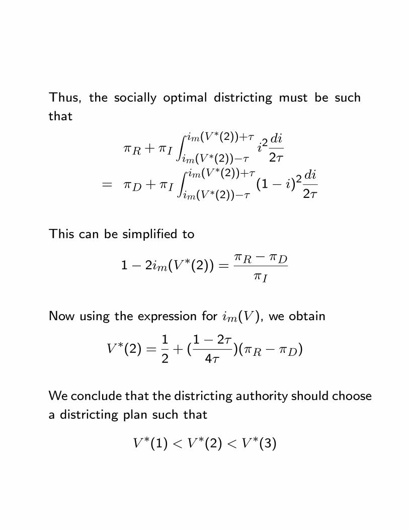
Thus, the socially optimal districting must be such

that

+

Z (∗(2))+

( ∗(2))−2

2

= +

Z (∗(2))+

( ∗(2))−(1− )2

2

This can be simplified to

1− 2( ∗(2)) = −

Now using the expression for ( ), we obtain

∗(2) = 1

2+ (

1− 24

)( − )

We conclude that the districting authority should choose

a districting plan such that

∗(1) ∗(2) ∗(3)

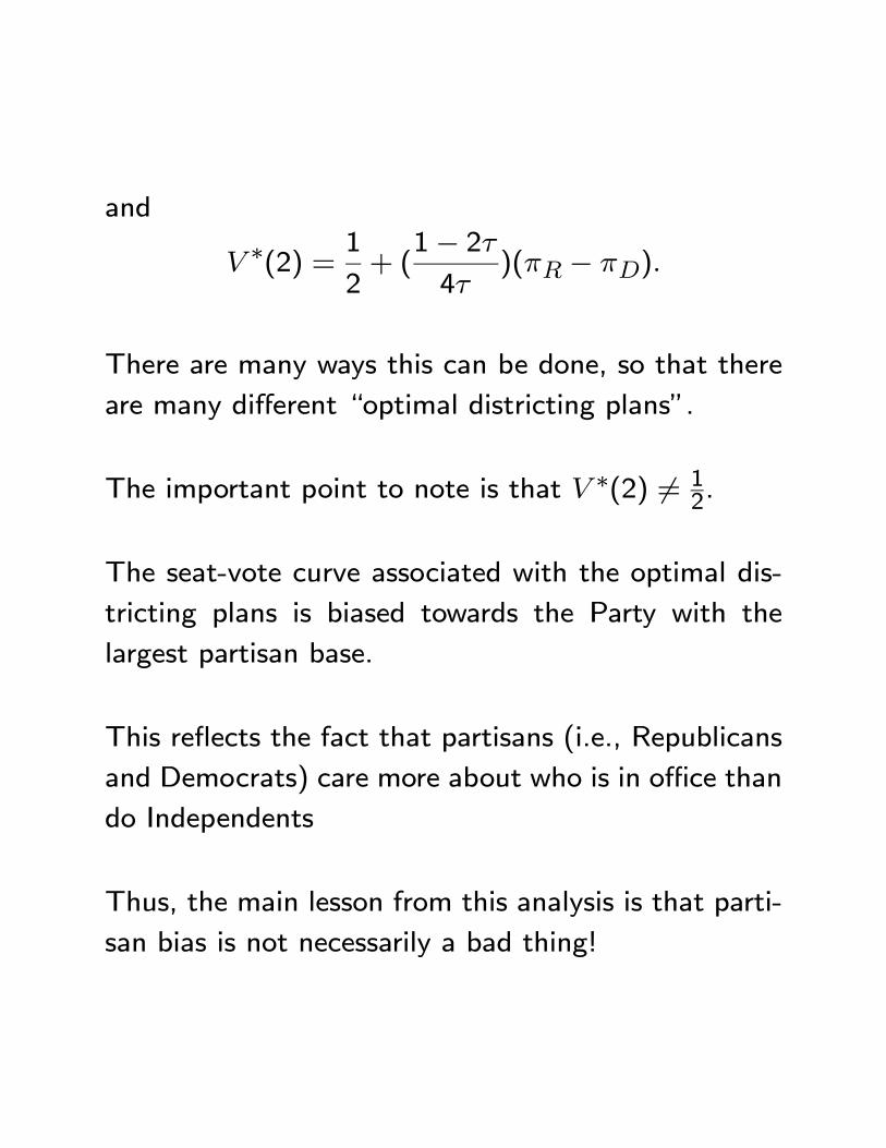
and

∗(2) = 1

2+ (

1− 24

)( − )

There are many ways this can be done, so that there

are many different “optimal districting plans”.

The important point to note is that ∗(2) 6= 12.

The seat-vote curve associated with the optimal dis-

tricting plans is biased towards the Party with the

largest partisan base.

This reflects the fact that partisans (i.e., Republicans

and Democrats) care more about who is in office than

do Independents

Thus, the main lesson from this analysis is that parti-

san bias is not necessarily a bad thing!

Coate and Knight (2007)

Coate and Knight (2007) study socially optimal dis-

tricting under the assumption that the policy out-

comes chosen by the legislature depend upon the aver-

age ideology of the legislators rather than the median

ideology.

They do this for two reasons:

i) to square with the political science literature which

focuses on the global properties of the seat vote curve

rather than its behavior in the neighborhood in which

( ) = 12.

ii) because there is empirical evidence from the U.S.

states that policy outcomes are sensitive to the frac-

tion of seats controlled by each party.

The districting problem is more involved under this as-

sumption because social welfare depends on the criti-

cal vote shares of all the districts rather than just the

median district.

They also compare empirically the actual seat-vote

curves from the U.S. states with those that would be

generated by socially optimal districtings.

This allows them to evaluate quantitatively the gains

from socially optimal districting.

Besley and Preston (2007)

Our analysis of socially optimal districting also em-

bodies a very spartan conception of electoral com-

petition - parties just put up candidates representing

their ideology and voters vote.

Parties and candidates therefore have no strategic choices

to make.

Intuitively, however, one might imagine that district-

ing would influence the type of candidates parties put

up and/or the platforms that parties run on.

In this case, an optimal districting would have to take

into account the implications for strategic choices.

Besley and Preston (2007) is a very interesting study

using U.K. data which relates to this general issue.

They argue first theoretically that the degree of par-

tisan bias in districting should impact the platforms

that parties run on.

They then investigate this prediction empirically using

data on U.K. local governments.

Valence and districting

Our analysis of socially optimal districting assumes

that all districting determines is the ideology of the

legislature.

One might also think of districting being important in

determining the average valence characteristics (com-

petence, honesty, etc) of legislators.

Imagine that candidates differ in both their ideology

and quality as measured by ∈ [0 max].

Assume that if the median legislator has ideology 0

and the average legislator quality is , a citizen with

ideology experiences a payoff given by −(− 0)2.

Assume as before that Democratic candidates have

ideology 0 and Republican candidates have ideology

1.

Let denote the quality of Party ’s candidate

( ∈ {}) in district .

Assume that is the realization of a random variable

with support [0 max] and CDF ().

Further assume that max implying that partisan

voters vote on the basis of ideology.

The key point to note about this environment is that

expected quality of the winning candidate is increasing

in the competitiveness of the district.

This is because Independent voters vote more on the

basis of quality and partisan voters vote on the basis

of ideology.

If the partisan votes cancel each other the race is more

likely to be determined by quality.

This gives a reason to make districts competitive.

It would be interesting (but hard) to solve for socially

optimal districting plans in this environment.

Polarization and districting

It is common to argue that districting is responsible for

the growing polarization that is observed in American

federal politics.

The intuitive idea is that there are too many safe dis-

tricts and that those districts elect more extreme can-

didates.

The safe districts are created by bipartisan gerryman-

dering which seeks to help out incumbents.

To capture this idea we would need a model where

the ideology of the candidates that the two parties

run depends on the characteristics of the district.

We would also need a model of legislative decision-

making that captured the difficulties that polarization

appears to cause.

This may be possible to do, but is much more com-

plicated.

It should also be noted that the idea that districting

causes polarization is not shared by most specialists

on American politics.

The reason is because the Senate has also become

more polarized over time and Senators represent states

and not districts.

In any case, there is probably scope for work on this

issue.

IV.2 Citizens’ Initiatives

In more than half of U.S. States, the constitution al-

lows citizens to place legislation directly on the ballot

for voters to approve.

Such a piece of legislation is known as a citizens’ ini-

tiative.

Examples of recent citizens’ initatives include propos-

als to legalize marijuana (in Alaska); create voucher

programs (in California); prohibit same-sex marriages

(numerous states); eliminate affirmative action in pub-

lic universities (California and Texas); require back-

ground checks at gun shows (Colorado); increase min-

imum wage (Florida).

To get an initiative placed on the ballot, it is necessary

to present a petition signed by some fraction of the

registered voters in the state in question.

The fraction varies across states, but ranges between

2-15% or registered voters.

Initiatives were first introduced in South Dakota in

1898 and were associated with the populist movement

in the late nineteenth century.

Most states which have them introduced them in the

early 1900s.

There were 360+ statewide initiatives over the 10

year period from 1995-2004 - over 30% in California,

Washington and Oregon.

A large amount of money is spent trying to get initia-

tives passed or blocked.

In 2004, gambling interests spent $90 million in Cali-

fornia on two ballot measures alone.

There is considerable debate about the role of initia-

tives - in particular, are they a good idea?

There is a large academic literature on the topic (see

Matsusaka’s papers on the reading list for discussion).

This literature seeks to understand what impact ini-

tiatives have on policy choices and whether they are

a good idea.

It is popularly believed that permitting citizens’ ini-

tiatives improves the “congruence” between citizens’

preferences and policy outcomes across the spectrum

of issues on which initiatives may be brought.

This premise is accepted by both advocates and op-

ponents of initiatives, with the main debate focusing

on the desirability of allowing voters’ opinions more

weight.

This premise receives backing from a variety of acad-

emic sources.

One nice example is Elizabeth Gerber’s 1996 paper

“Legislative Response to the Threat of Popular Initia-

tives”.

She begins with a simple game theoretic model which

illustrates why initiatives might move policy closer to

the median voter’s ideal and then tests the idea em-

pirically.

We will begin our discussion of initiatives by going

through Gerber’s theory and evidence.

We will then discuss other evidence and relevant the-

oretical ideas.

Finally, we will come back to the question of whether

initiatives are good or bad.

IV.2.i Gerber’s paper

Gerber’s model

There are three players: an incumbent politician ; an

interest group ; and a representative voter .

There is a one dimensional policy ∈ [0 1]

The preferences of the three players are

() = − | − |() = − | − |

() = − | − |where is money and 0.

Thus, players have distance preferences, with ideal

points , , and .

It is assumed that , so that the politician

prefers a lower level of the policy, than does the voter

and the interest group prefers a higher level.

Game

The interaction between the players has three stages.

Stage 1. The politician selects a policy level .

Stage 2. The interest group decides whether to pro-

pose an initiative - it costs the interest group to

propose.

This cost represents the cost of collecting the required

signatures on the petition.

Let denote the proposed policy level in the initiative.

Stage 3. If no initiative is proposed, the policy out-

come is simply .

If an initiative is proposed, the voter chooses whether

to approve it.

If he does approve it, the policy outcome is , and if

he does not, the policy outcome is .

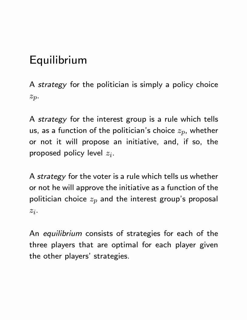
Equilibrium

A strategy for the politician is simply a policy choice

.

A strategy for the interest group is a rule which tells

us, as a function of the politician’s choice , whether

or not it will propose an initiative, and, if so, the

proposed policy level .

A strategy for the voter is a rule which tells us whether

or not he will approve the initiative as a function of the

politician choice and the interest group’s proposal

.

An equilibrium consists of strategies for each of the

three players that are optimal for each player given

the other players’ strategies.

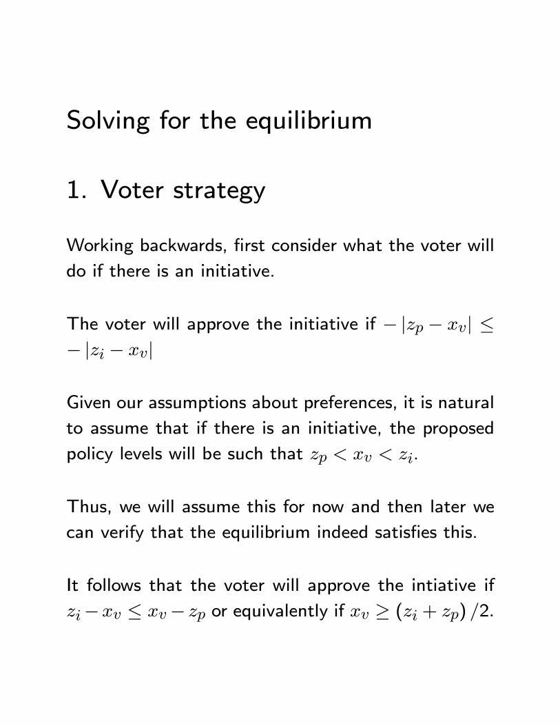
Solving for the equilibrium

1. Voter strategy

Working backwards, first consider what the voter will

do if there is an initiative.

The voter will approve the initiative if − | − | ≤− | − |

Given our assumptions about preferences, it is natural

to assume that if there is an initiative, the proposed

policy levels will be such that .

Thus, we will assume this for now and then later we

can verify that the equilibrium indeed satisfies this.

It follows that the voter will approve the intiative if

− ≤ − or equivalently if ≥ ( + ) 2

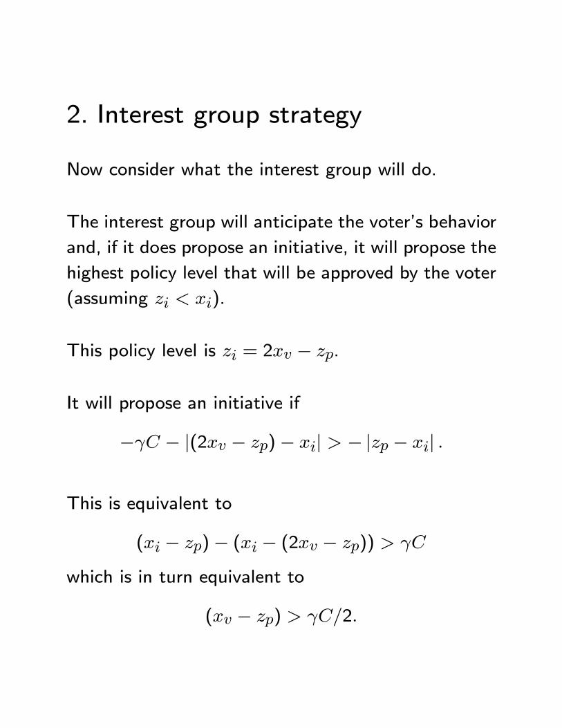
2. Interest group strategy

Now consider what the interest group will do.

The interest group will anticipate the voter’s behavior

and, if it does propose an initiative, it will propose the

highest policy level that will be approved by the voter

(assuming ).

This policy level is = 2 − .

It will propose an initiative if

− − |(2 − )− | − | − |

This is equivalent to

( − )− ( − (2 − ))

which is in turn equivalent to

( − ) 2

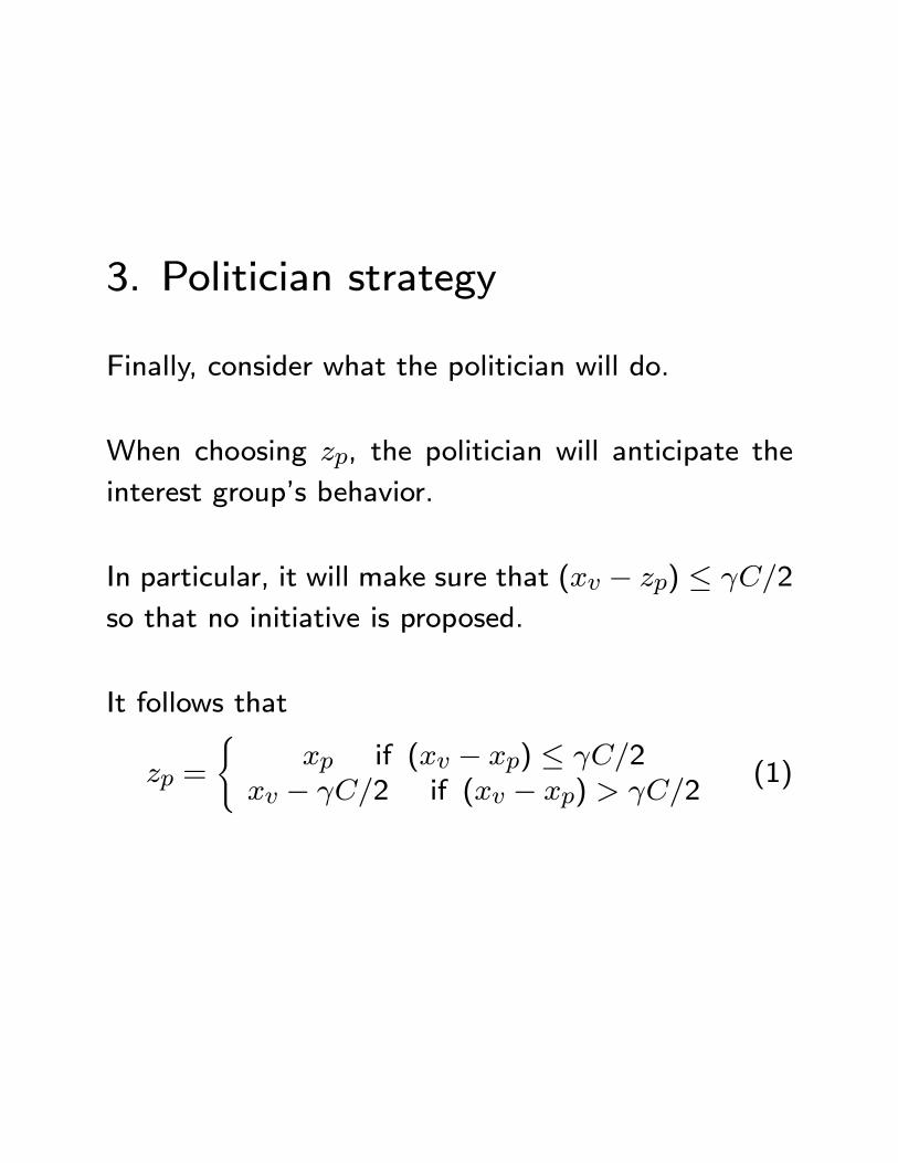
3. Politician strategy

Finally, consider what the politician will do.

When choosing , the politician will anticipate the

interest group’s behavior.

In particular, it will make sure that ( − ) ≤ 2

so that no initiative is proposed.

It follows that

=

( if ( − ) ≤ 2

− 2 if ( − ) 2(1)

Equilibrium outcome

The outcome of the game is that the politician will

choose as described in (2) and no initiative will be

proposed.

Assuming that 2 ( − ) , the threat of the

initiative will bring the politician’s choice closer to the

voter’s ideal point.

The initiative therefore has an effect on policy even

though it is not actually used.

If we extend the model to incorporate different beliefs

on the part of the politician and interest group on the

location of the voter’s ideal point (i.e., ), we can

have initiatives actually being used.

Gerber’s empirical work

Gerber tests the theoretical idea using data on parental

consent notification laws for abortion.

As of 1990, 24 states required parental consent noti-

fication for women aged 18 or younger.

All of these laws were passed by state legislatures as

opposed to initiatives.

These consent requirements are a good policy to look

at because:

(i) states have primary jurisdiction

(ii) legislatures play a role

(iii) survey data is available state-by-state on voters’

preferences on the topic.

Gerber runs regressions of the form:

Pr( = ) =exp(0+1+2+3·)

1+exp(0+1+2+3·)

where is a measure of the median voter’s preference

in state ; is a vector of state characteristics; and

is a state dummy variable for whether the state has

the initiative.

She finds that 2 is positive and significant.

This suggests that policy is closer to voters’ prefer-

ences in states with the inititiative.

She does the same thing for the death penalty with

similar results.

IV.2.ii Other evidence and related the-ory

Evidence

Evidence comparing fiscal policies in states with and

without initiatives is also supportive of the general

idea that the initiative improves the “congruence” be-

tween citizens’ preferences and policy outcomes.

Matsusaka in a 2005 paper in the Journal of Eco-

nomic Perspectives reviews evidence on the effect of

the initiative on taxes and spending.

More than 10 studies have found that initiative states

spent and taxed less than noninitiative states begin-

ning around the mid 1970s, controlling for demographic

and political factors.

The estimates imply that the initiative cut the com-

bined spending of state and local governments by

about 5% and cut state government spending by over

10%.

Initiative states also tend to decentralize spending from

state to local governments and shift revenue out of

broad-based taxes into user fees and charges for ser-

vices.

Surveys of voter preferences suggest that these moves

are in the direction in which the majority of voters

prefer.

Theory

In light of all this evidence, a natural question to ask

is why elections are not by themselves sufficient to

bring policies into line with what the majority of voters

want.

For example, Gerber’s model assumes that the in-

cumbent politician’s preferences are different from the

voter’s.

One may well ask why the voters would have elected

such an incumbent in the first place or why they can-

not just toss the incumbent out of office if he chooses

to ignore their preferences.

In a sense, we have already answered this with those

models of elections reviewed in Section I.2 which do

not predict median voter outcomes.

However, there are some additional points that can

be made on this which are particularly relevant for

thinking about the impact of initiatives.

1) Corruption

Elections may provide voters with very little control

when incumbent politicians are receiving some finan-

cial reward in return for ignoring voters’ preferences.

When initiatives were first introduced there was a

great deal of concern about corruption at the state

level.

Legislators were literally being bribed to do the bidding

of corporations.

This problem could not be resolved via elections be-

cause any candidate who was elected would succumb

to the same temptations.

To see this formally, imagine a citizen-candidate model

of elections followed by a common agency model of

influence with a single interest group.

If all potential candidates are willing to trade policy for

money, there is no way to prevent the interest group

from influencing policy via elections.

The only way round this problem is to take legislation

out of the control of state legislatures.

2) The multi-dimensional nature ofpolitical competition

While most of our models of elections have ignored

this point, it is important to note that when voters

are voting on candidates, they are typically voting on

a bundle of different policy positions.

Even in very competitive elections with no corruption,

there is no reason to suppose that a candidate has to

agree with the majority of voters on every issue to get

elected.

Many issues are not salient in elections and candidates

can hold non-majoritarian positions with no electoral

penalty.

For example, trade policy: most voters tend to be very

protectionist, but elected leaders in both parties tend

to promote free trade.

The reason is that very few people are actually voting

on this issue.

Other issues are only salient for those with the minor-

ity view.

For example, affirmative action and gun control.

In this case, the electoral incentive is for candidates

not to champion the majority view.

Because the minority votes on the issue and the ma-

jority votes on other issues.

In these cases, if the voters have access to initiatives

and the cost of placing an initiative is not too large,

congruence on an issue can be restored.

The key feature of initiatives is that they allow voters

to unbundle issues and force a direct vote on that

issue alone.

Besley and Coate (2008) try to formalize this argu-

ment in a model in which two parties compete by se-

lecting citizen-candidates and the winning candidate

must choose two distinct policies.

They show that allowing citizens’ initiatives on one of

the issues improves congruence on this issue relative

to candidate elections alone.

IV.2.iii Are initiatives good or bad?

In general it is difficult to say whether initiatives are

good or bad since there is nothing necessarily good or

bad from a social welfare perspectiive about having

congruence on an issue-by-issue basis.

In particular, as we have argued Section III.2, it could

be the case that on a specific issue the minority feels

much more intensely about the issue (for example, gay

marriage) than the majority and social welfare would

be maximized by respecting the minority’s preference.

An additional criticism - usually from elite groups -

concerns the lack of voter information.

The reason for representative democracy is so that we

can delegate decisions to a few professionals who have

the time to find out the right thing to do.

Voters are rationally ignorant about issues.

Thus, majoritarian choices on complex initiatives may

be misguided.

This is particularly so if monied interests can fool vot-

ers to voting against their interests through slick ad-

vertising campaigns, etc.

Advocates of initiatives argue that while indeed voters

do not understand all the details of every initiative,

they do not need to.

They can take cues from the positions of interest

groups, newspaper endorsements, etc.

There is quite a bit of evidence in support of this idea

as we discussed in Section I.1.

A final criticism is that initiatives take a huge amount

of resources.

First, all the signatures have to be collected to get an

issue on the ballot and second, in the campiagn stage,

a huge amount of resources are spent on advertising.

These expenditures could be seen as wasteful - dissi-

pating any benefit from aligning policy more closely

with majoritarian preferences.

IV.3 Campaign Finance Policy

How should campaigns be financed?

Should private campaign contributions be regulated?

Should public money be used and, if so, how should

it be allocated to candidates?

These are interesting questions on which there is little

consensus.

Some commentators argue that all that is necessary is

to have disclosure requirements which require candi-

dates to publicly announce who is giving them money

and in what amounts.

Others argue for full public financing whereby taxpayer

dollars are allocated to qualifying candidates.

Still others argue for a voucher scheme whereby all

citizens receive a small budget (say, $100) that they

can allocate to political candidates.

IV.3.i Background

Recall from Section I.5 that campaign contributions

to candidates for federal office are made by individual

citizens and Political Action Committees (PACs).

Interest groups, unions, and corporations contribute

through PACs.

The amount that individuals and PACS can give to

any one candidate is limited.

The individual limit per candidate is $2500 per elec-

tion and the PAC limit per candidate is $5000 per

election.

There are also limits on how much individuals and

PACs can give to national parties and to other PACs.

There are no limits on the total amount of campaign

spending that candidates can do - such limits have

been ruled unconstitutional by the Supreme Court.

There are disclosure requirements for candidates and

parties.

They must identify the PACs that provide them contri-

butions, and the names, occupations, employers, and

addresses of all individual contributors who give them

more than $200.

They must also disclose exactly how they spend the

money they get.

Since the Supreme Court’s 2010 Citizens United vs

the FEC decision, interest groups, unions, and cor-

porations are free to spend whatever they want on

political advertisements.

Thus, for example, they can run ads telling people

their opinions about particular candidates.

This expenditure is treated differently from contribu-

tions to candidates and is protected as free speech.

At the federal level, public funding is limited to sub-

sidies for presidential candidates.

These subsidies are available for both primaries and

the general election.

However, they come with a catch: in return for re-

ceiving the taxpayer dollars, candidates must agree to

limit their spending.

In the 2008 presidential election, most of the major

candidates opted out of the public financing scheme

for the primaries.

Moreover, Barack Obama opted out of the scheme for

the general election as well.

The public financing scheme is funded by a $3 tax

check off on individual tax returns.

In 2006 fewer than 8% of taxpayers checked this box

(even though it means no increase in their tax bills),

leaving the public financing fund a little short of funds.

Races for non-federal offices are governed by state and

local law.

Over half the states allow some level of corporate and

union contributions.

Some states have limits on contributions that are more

stringent than national limits.

Six states (IL, MO, NM, OR, UT, VA) have no limits

at all.

Public financing schemes are more common at the

state and local level.

One method is the Clean Money, Clean Elections pro-

gram.

To qualify for receiving money, candidates must first

raise a target amount privately in small contributions.

Once they have done this, they receive an amount

from the program.

In return, they are not allowed to accept further pri-

vate contributions or to use their own money.

However, if they are running against a candidate who

is not participating in the scheme and outspending

them, they are eligible to receive additional funds from

the program.

This program is currently used in Arizona and Maine.

It was proposed for California in a citizens’ initiative,

but the initiative failed.

In addition, the constitutionality of that part of the

program that provides additional funds is problematic

and in June 2011 the Supreme Court struck down this

part of the program.

The ruling will likely be bad for the future of the pro-

gram.

If additional funds are not granted, candidates may

well opt out of the program to avoid being outspent.

This is what we have seen recently for the presidential

public financing scheme.

IV.3.ii Economic analysis of campaignfinance policy

From an economic perspective, a basic question is

how well an unregulated system of campaign giving

will perform from a social welfare perspective.

This depends critically on what we think the resources

spent by candidates are used for.

As we discussed in Section I.5, there are two main

ways to think about campaign spending.

First, spending buys the votes of “noise voters”.

Recall that noise voters are voters who are voting for

random non-policy related reasons.

Campaign advertising is simply assumed to attract

these voters.

Second, spending allows candidates to provide infor-

mation about their positions and qualifications to un-

informed voters.

In this view, voters are rational and update their be-

liefs based on the information they are provided by

campaigns.

1. The noise-voter perspective

Under this perspective, campaign spending tends to

either distort policy in an undesirable way or to just

be wasteful rent-seeking with no policy consequences.

Limiting contributions therefore tends to be a good

idea.

We can illustrate the implications of the perspective

with Grossman and Helpman’s (1996) analysis which

embeds the common agency model within a theory of

electoral competition.

The model assumes that campaign contributions “buy”

the votes of noise voters and endogenizes the level of

contributions via the common agency model.

It is a useful model to know about independent of its

implications for campaign finance policy.

The voting population is divided into groups indexed

by ∈ {1 }.

The fraction of the population in group is .

There are two candidates, indexed by ∈ {}.

Following Lindbeck-Weibull, candidates compete by

staking out positions on “pliable” policies and have

fixed positions with respect to “non-pliable” policies.

Let denote candidate ’s positions on the pliable

polices and let be the set of possible positions.

Voters are divided into two types - rational and noise

- the fraction of rational voters is .

≤ of the citizen groups are represented by inter-

est groups - let () denote the group represented by

interest group ∈ {1 }

The interest groups give the candidates contributions

that are used to buy the votes of the noise voters.

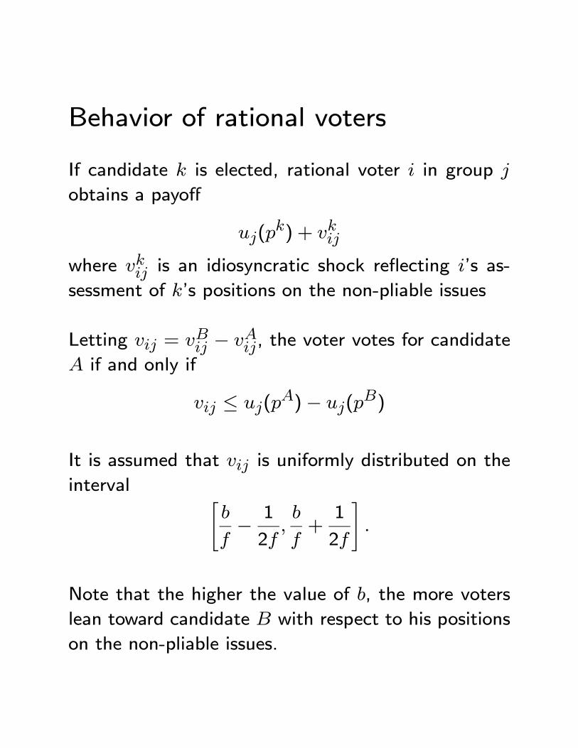
Behavior of rational voters

If candidate is elected, rational voter in group

obtains a payoff

() +

where is an idiosyncratic shock reflecting ’s as-

sessment of ’s positions on the non-pliable issues

Letting = − , the voter votes for candidate

if and only if

≤ ()− (

)

It is assumed that is uniformly distributed on the

interval "

− 1

2

+1

2

#

Note that the higher the value of , the more voters

lean toward candidate with respect to his positions

on the non-pliable issues.

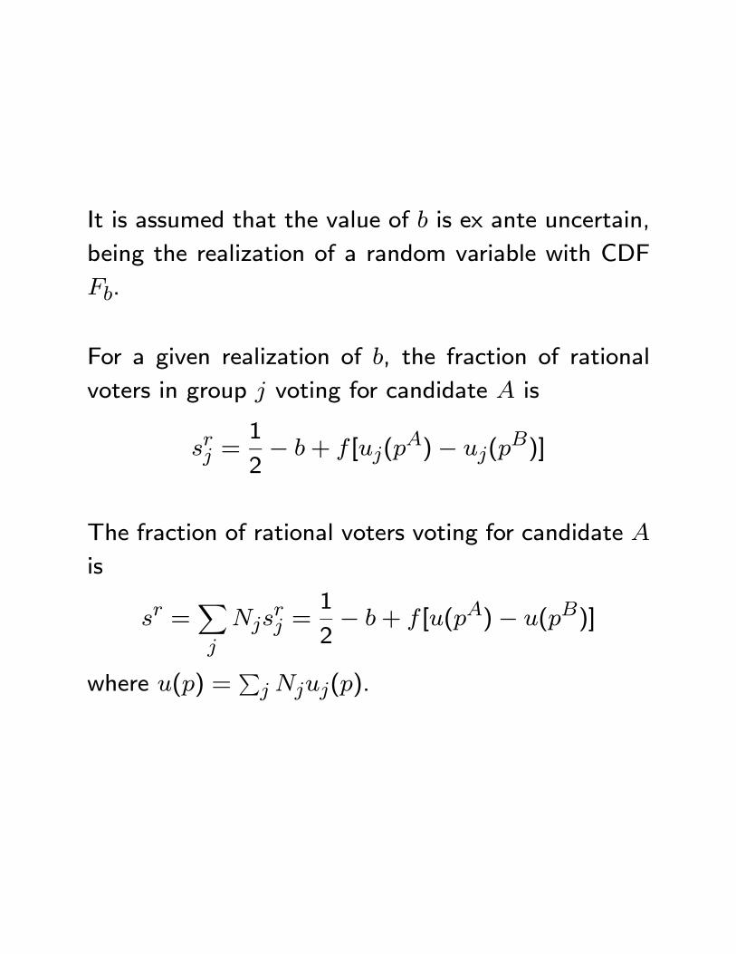
It is assumed that the value of is ex ante uncertain,

being the realization of a random variable with CDF

.

For a given realization of , the fraction of rational

voters in group voting for candidate is

=1

2− + [(

)− ()]

The fraction of rational voters voting for candidate

is

=X

=

1

2− + [()− ()]

where () =P ().

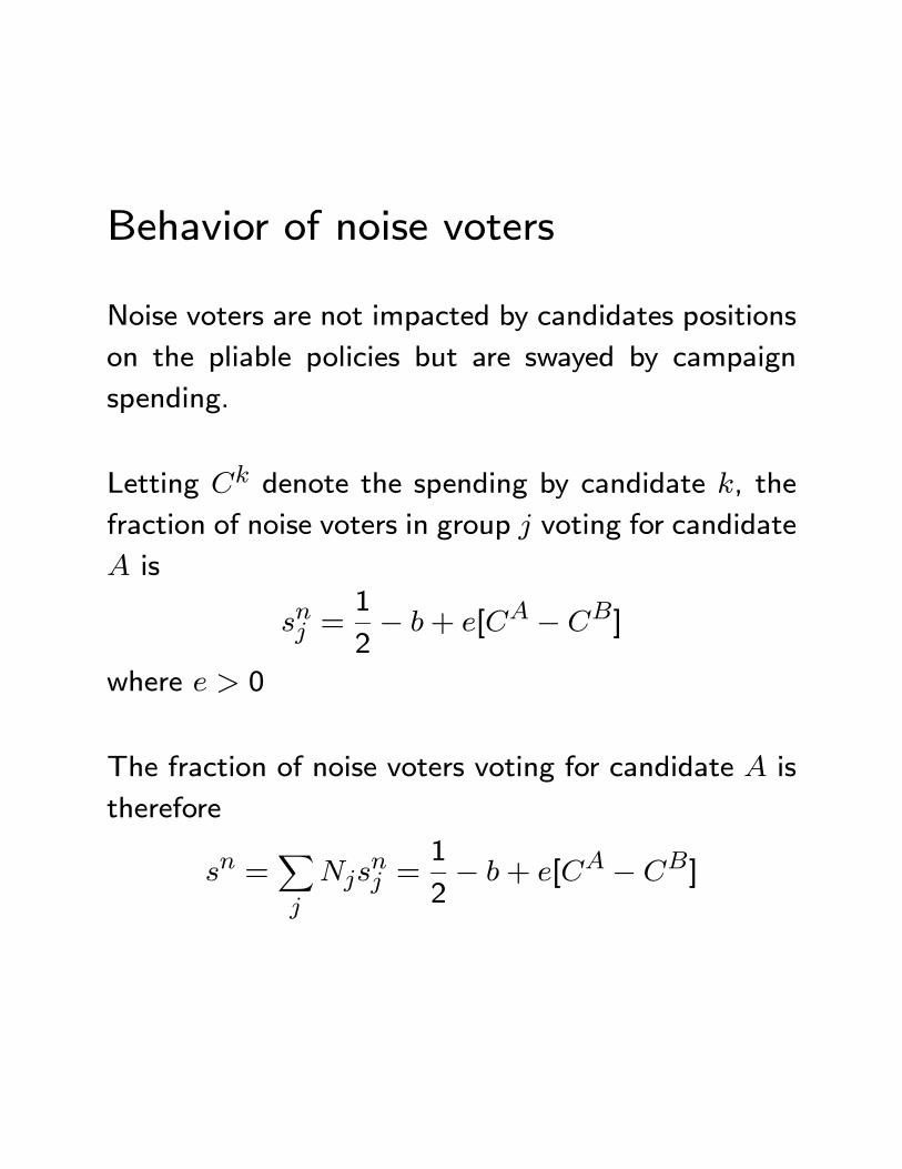
Behavior of noise voters

Noise voters are not impacted by candidates positions

on the pliable policies but are swayed by campaign

spending.

Letting denote the spending by candidate , the

fraction of noise voters in group voting for candidate

is

=1

2− + [ − ]

where 0

The fraction of noise voters voting for candidate is

therefore

=X

=

1

2− + [ − ]

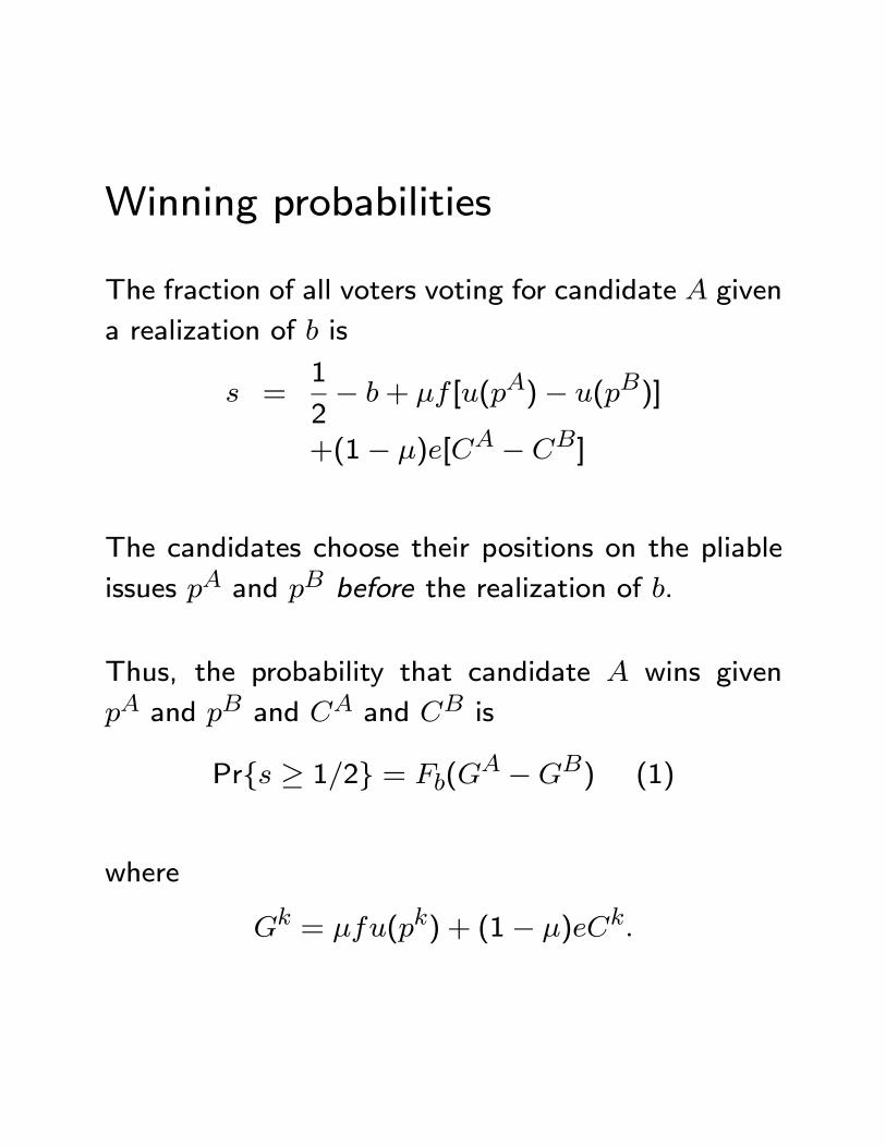
Winning probabilities

The fraction of all voters voting for candidate given

a realization of is

=1

2− + [()− ()]

+(1− )[ − ]

The candidates choose their positions on the pliable

issues and before the realization of .

Thus, the probability that candidate wins given

and and and is

Pr{ ≥ 12} = ( −) (1)

where

= () + (1− )

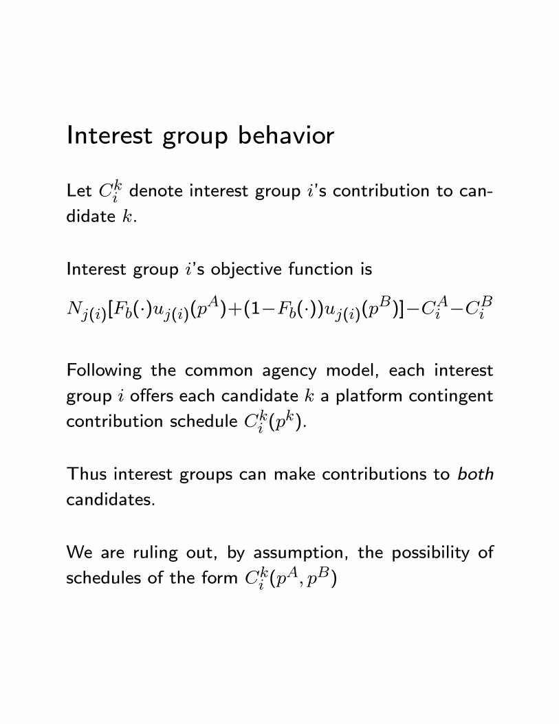
Interest group behavior

Let denote interest group ’s contribution to can-

didate .

Interest group ’s objective function is

()[(·)()()+(1−(·))()()]− −

Following the common agency model, each interest

group offers each candidate a platform contingent

contribution schedule (

).

Thus interest groups can make contributions to both

candidates.

We are ruling out, by assumption, the possibility of

schedules of the form (

)

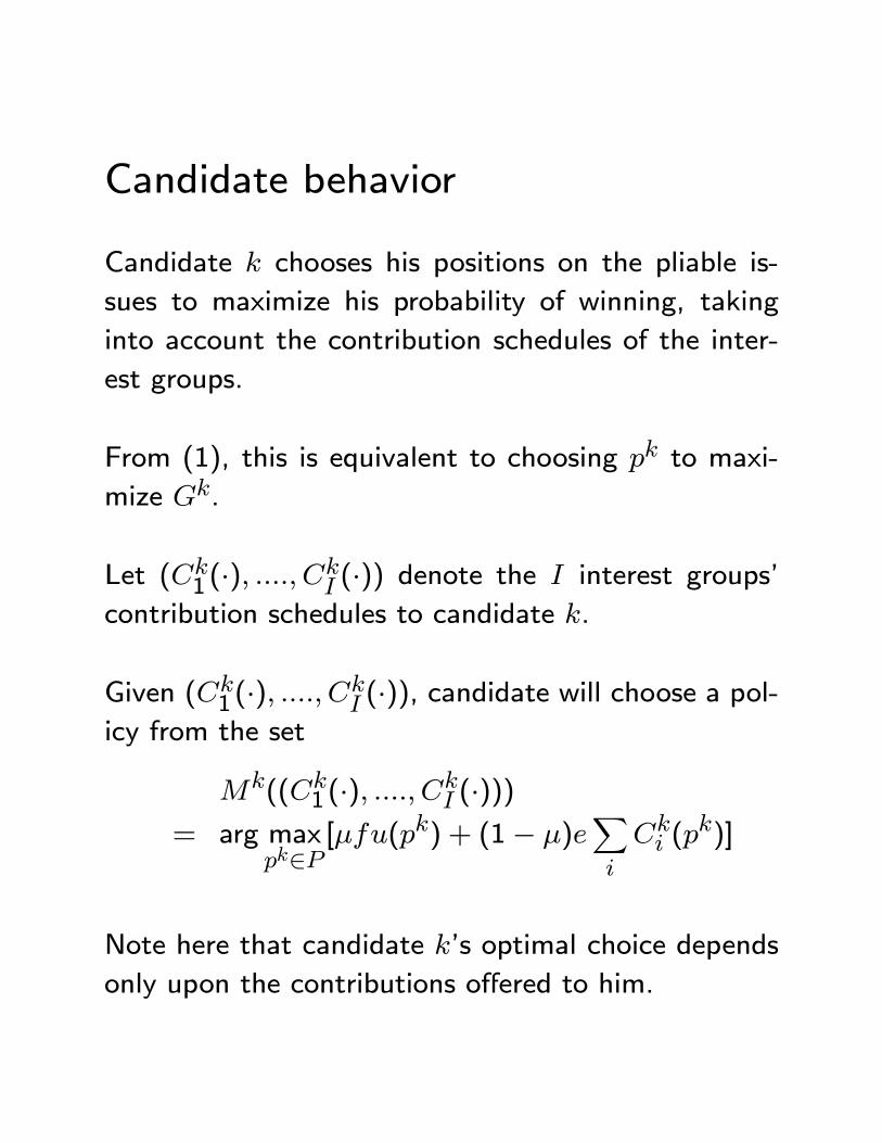
Candidate behavior

Candidate chooses his positions on the pliable is-

sues to maximize his probability of winning, taking

into account the contribution schedules of the inter-

est groups.

From (1), this is equivalent to choosing to maxi-

mize .

Let (1 (·)

(·)) denote the interest groups’

contribution schedules to candidate .

Given (1 (·)

(·)), candidate will choose a pol-icy from the set

((1 (·)

(·)))= arg max

∈[() + (1− )

X

(

)]

Note here that candidate ’s optimal choice depends

only upon the contributions offered to him.

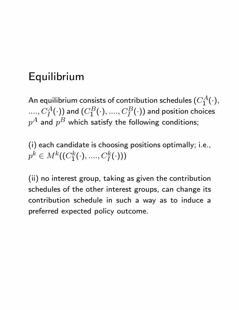
Equilibrium

An equilibrium consists of contribution schedules (1 (·)

(·)) and (

1 (·) (·)) and position choices

and which satisfy the following conditions;

(i) each candidate is choosing positions optimally; i.e.,

∈((1 (·)

(·)))

(ii) no interest group, taking as given the contribution

schedules of the other interest groups, can change its

contribution schedule in such a way as to induce a

preferred expected policy outcome.

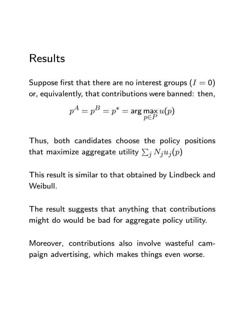
Results

Suppose first that there are no interest groups ( = 0)

or, equivalently, that contributions were banned: then,

= = ∗ = argmax∈

()

Thus, both candidates choose the policy positions

that maximize aggregate utilityP ()

This result is similar to that obtained by Lindbeck and

Weibull.

The result suggests that anything that contributions

might do would be bad for aggregate policy utility.

Moreover, contributions also involve wasteful cam-

paign advertising, which makes things even worse.

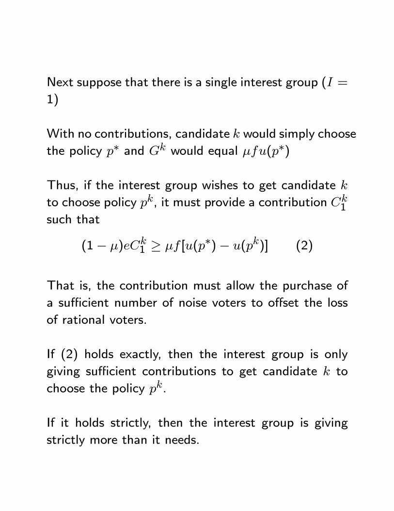
Next suppose that there is a single interest group ( =

1)

With no contributions, candidate would simply choose

the policy ∗ and would equal (∗)

Thus, if the interest group wishes to get candidate

to choose policy , it must provide a contribution 1

such that

(1− )1 ≥ [(∗)− ()] (2)

That is, the contribution must allow the purchase of

a sufficient number of noise voters to offset the loss

of rational voters.

If (2) holds exactly, then the interest group is only

giving sufficient contributions to get candidate to

choose the policy .

If it holds strictly, then the interest group is giving

strictly more than it needs.

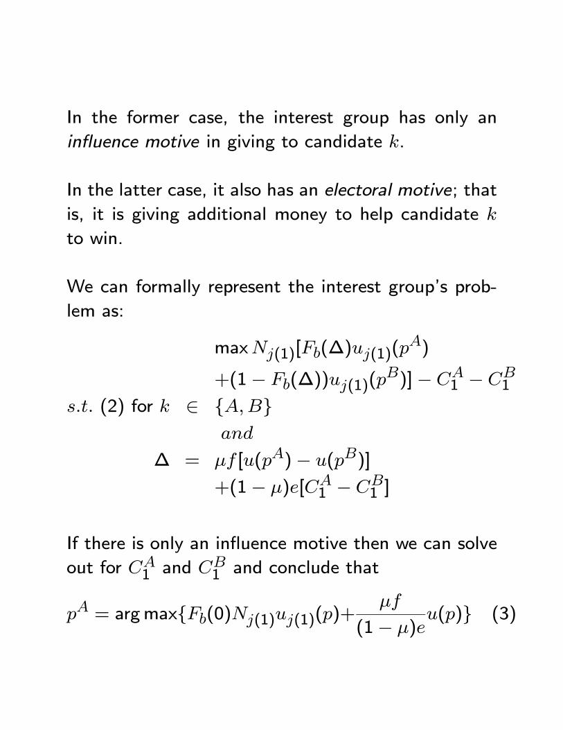
In the former case, the interest group has only an

influence motive in giving to candidate .

In the latter case, it also has an electoral motive; that

is, it is giving additional money to help candidate

to win.

We can formally represent the interest group’s prob-

lem as:

max(1)[(∆)(1)()

+(1− (∆))(1)()]−

1 − 1

(2) for ∈ {}

∆ = [()− ()]

+(1− )[1 −

1 ]

If there is only an influence motive then we can solve

out for 1 and

1 and conclude that

= argmax{(0)(1)(1)()+

(1− )()} (3)

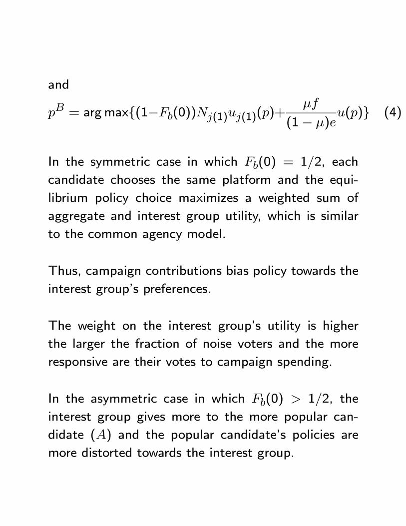
and

= argmax{(1−(0))(1)(1)()+

(1− )()} (4)

In the symmetric case in which (0) = 12, each

candidate chooses the same platform and the equi-

librium policy choice maximizes a weighted sum of

aggregate and interest group utility, which is similar

to the common agency model.

Thus, campaign contributions bias policy towards the

interest group’s preferences.

The weight on the interest group’s utility is higher

the larger the fraction of noise voters and the more

responsive are their votes to campaign spending.

In the asymmetric case in which (0) 12, the

interest group gives more to the more popular can-

didate () and the popular candidate’s policies are

more distorted towards the interest group.

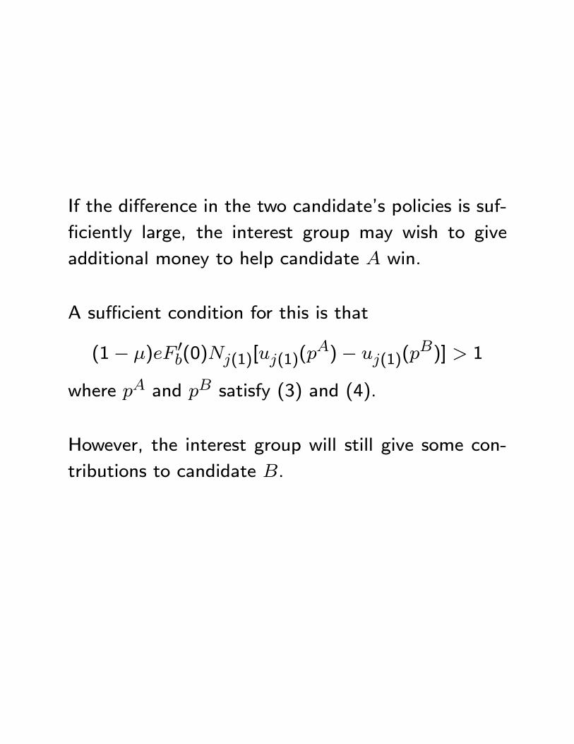
If the difference in the two candidate’s policies is suf-

ficiently large, the interest group may wish to give

additional money to help candidate win.

A sufficient condition for this is that

(1− ) 0(0)(1)[(1)()− (1)(

)] 1

where and satisfy (3) and (4).

However, the interest group will still give some con-

tributions to candidate .

Finally, suppose there are multiple interest groups.

While the model gets fairly intractable, it does yield

three insights.

First, there is the possibility of multiple equilibria -

some with candidate getting the most contributions

and some with candidate .

The expectation that a candidate will attract most of

the funds is self-fulfilling.

Second, it is unlikely that the electoral motive will be

operative for more than one interest group.

This reflects a free-rider problem in contributing with

an electoral motive.

Third, when (i) only the influence motive is opera-

tional for all interest groups; (ii) all the interest groups

employ differentiable contribution schedules; and (iii)

() is strictly concave for all , then we have that

= argmax{( −)X

()()()

+

(1− )()}

and

= argmax{(1− ( −))

X

()()()

+

(1− )()}

Thus, again, the platforms maximize a weighted sum

of interest group and aggregate utility.

The indeterminacy in the model is with respect to

− which determines the advantage of each

candidate.

Note that if interest groups are representative of the

populationP ()()() will be similar to (),

and campaign spending will not distort policy.

However, the campaign spending is itself completely

wasteful, so it is still optimal to ban it.

2. The informative campaignspending perspective

The Grossman-Helpman model generates some useful

insights.

However, the noise-voter perspective seems overly sim-

plistic and cynical.

In reality, it does seem that campaign spending plays

a role in allowing candidates to provide information

to voters about their (and their opponents’) positions

on the issues; qualifications for office; and plans for

action.

Such information could lead voters to elect better can-

didates which could lead to aggregate social benefits.

Unfortunately, developing the implications of this in-

formative campaign spending view is more compli-

cated, since we have to model how information is

transmitted during the campaign.

I will describe one way of modelling this and discuss

the results that the model yields.

An informative campaign spending model

We use the same basic set-up that we have used sev-

eral times before.

There are three types of voters: Democrats, Indepen-

dents, and Republicans.

Democrats and Republicans have ideologies 0 and 1,

respectively.

Independents have ideologies that are uniformly dis-

tributed on the interval [− + ] where 0

and is the realization of a random variable uni-

formly distributed on [12 − 12 + ], where ∈(0 ) and + 12.

The size of the population is and there are In-

dependents.

The non-Independents are equally divided between De-

mocrats and Republicans, so the model is symmetric.

The community is electing a representative.

Candidates are put forward by two political parties:

Party , comprised of Democrats and Party , com-

prised of Republicans.

Each party selects a candidate of its own ideology

but may select either a “qualified” ( = 1) or an

“unqualified” ( = 0) candidate.

The intuitive idea is that finding qualified candidates

is difficult, and a party may not be able to find one.

The probability that a party can find a qualified can-

didate is .

The payoff enjoyed by a citizen with ideology from

having a leader of ideology 0 and qualifications isgiven by −

¯̄− 0

¯̄.

, so that Democrats and Republicans prefer

a candidate of their own ideology, even when he is

unqualified.

Independents do not know whether each party’s can-

didate is qualified or unqualified.

Candidates can convey information concerning their

candidates’ qualifications via advertising.

To simplify, assume candidates can only advertise their

own candidates’ characteristics, ruling out negative

advertising.

Thus only qualified candidates can benefit from ad-

vertising.

If a candidate spends an amount , its message reaches

a fraction () of the population, where the function

is such that (0) = 0, 0() 0, and 00() 0.

Candidates’ advertising is financed by campaign con-

tributions provided by two interest groups - a Demo-

crat group that contributes to Party ’s candidate

and a Republican group that contributes to Party ’s.

Each group constitutes a fraction of the population.

Interest groups’ objectives are to maximize the ex-

pected payoff of their members.

Game

The timing of the model is as follows:

(i) Parties select candidates.

(ii) If their party’s candidate is qualified, interest groups

decide how much campaign contributions to give.

(iii) Candidates use their contributions to finance ad-

vertising.

(iii) Voters, having possibly observed one or both can-

didates’ advertisements, update their beliefs about

candidates’ qualifications and vote.

Equilibrium

Equilibrium in this model will consist of (i) campaign

contribution levels and that the two interest

groups make if their party’s candidate is qualified, and

(ii) a description of how voters behave.

The campaign contributions must be optimal for the

interest groups given how they expect voters behave

and voters behavior must be appropriately rational.

Given the symmetry of the model, we will study the

symmetric equilibrium in which = = .

Democrat and Republican voters always vote for the

candidate put forward by their party, so their behavior

is straightforward.

Independents may vote for either party’s candidate.

Independents behavior is straightforward when they

have either seen both candidates’ advertisements or

seen nothing from either candidate: they just vote for

the Democrat if their ideology is less than 12 and

the Republican otherwise.

The interesting case is when they have seen an adver-

tisement from one candidate (say the Democrat) and

not the other.

Then an Independent with ideology will vote for the

Democrat if

− ≥ − (1− )

where is the probability the voter assigns to the

unadvertised Republican candidate being qualified.

Rearranging the above inequality, we see that an In-

dependent with ideology will vote for the Democrat

if

≤ (1− )

2+1

2

If he had not seen the advertisement, he would vote

for the Democrat if ≤ 12.

Thus, advertising leads the advertised candidate to

get an extra slice of voters.

This is what gives the advertised candidate an advan-

tage.

The belief is determined as part of the equilibrium

and will take into account how likely it is that a voter

will miss seeing an advertisement if a candidate is

qualified.

In equilibrium, Bayesian updating implies

=[1− ()]

[1− ()] + (1− )

Results

In equilibrium, under appropriate assumptions, inter-

est groups will spend on behalf of their qualified can-

didates.

As a result of this spending, qualified candidates de-

feat unqualified opponents with a probability greater

than 12.

If there were no campaign spending, qualified candi-

dates would have no advantage over unqualified op-

ponents.

Since all citizens benefit from qualified candidates be-

ing more likely to hold office, campaign spending has

a social benefit.

In general, the level of campaign spending on behalf

of qualified candidates can be smaller or larger than

the level that maximizes a utilitarian social welfare

function.

There are two offsetting forces.

On the one hand, there remains the force arising in the

Grossman-Helpman model - the two groups spending

is purely wasteful when the two parties’ candidates

have the same qualifications.

This force leads campaign spending to be too high.

On the other hand, when choosing how much to spend

on behalf of qualified candidates, interest groups only

take into account the benefits to their members of

their candidate winning.

This force leads campaign spending to be too low.

Formally, it can be shown that as gets close to 1

there is necessarily too much campaign spending.

Intuitively, if both parties’ candidates are highly likely

to be qualified, there is little chance that we will be

in the situation in which campaign spending can be

socially beneficial; i.e., one candidate qualified and the

other unqualified.

Similarly, as gets close to zero, there is too much

campaign spending.

This is because there is little gain from having a quali-

fied candidate in office rather than an unqualified can-

didate.

Campaign spending is more likely to be underprovided,

the larger is , the larger is , and the smaller is .

All in all, the model provides a logical foundation for

believing that unregulated campaign spending may be

too low.

It therefore provides a possible justification for policies

that subsidize campaign giving, like tax deductions.

Favors and public financing

The above model assumes that campaign contribu-

tions are provided by interest groups for purely ideo-

logical reasons.

Many of the arguments in favor of limits or public

financing are worried about the quid-pro-quo of can-

didates providing policy favors for their contributors

once they are elected.

Policy favors are things like special tax breaks or reg-

ulatory exemptions which benefit interest groups but

are paid for by regular citizens.

The aggregate cost of these favors exceeds the bene-

fits they provide, so that they are a net loss to society.

As we saw in Section I.5, the evidence of a quid-pro-

quo is not particularly strong.

On the other hand, giving to federal candidates is

already heavily regulated so who can say what would

happen without such regulations.

It seems highly likely that quid-pro-quo would arise in

an unregulated system.

Thus, it is interesting to think about what might hap-

pen in an unregulated system with policy favors.

Coate (2004) argues that in such a world campaign

finance policy, in the form of contribution limits and

public matching grants, can be Pareto improving.

To see the argument, we just need to modify the above

model to allow policy favors.

Specifically, assume that after selection, each party’s

candidate (if qualified) requests a contribution from

his interest group and that, to obtain a larger contri-

bution, a candidate can offer to implement favors if

elected.

When a candidate implements a level of favors each

interest group member enjoys a monetary benefit ()

at a cost to every citizen, where (0) = 0 and is

increasing and strictly concave.

In addition, () ≤ for all (so favors create no

aggregate benefits) and 0() 1.

Each interest group agrees to a candidate’s request

only if it benefits it to do so.

Also so we can vary candidate incentives to offer fa-

vors, assume candidates obtain a non-policy related

payoff 0 from holding office.

Higher makes candidates more power hungry and

hence more willing to grant favors.

The timing of the extended model is as follows:

(i) Parties select candidates.

(ii) If qualified, candidates request contributions from

their interest groups and promise favors in exchange.

(iii) Candidates use their contributions to finance ad-

vertising.

(iv) Voters, having possibly observed one or both can-

didates’ advertisements, update their beliefs about

candidates’ qualifications and vote.

Voters do not observe the amount of favors promised,

but do have rational expectations.

(v) The winning candidate chooses policy and imple-

ments favors.

Equilibrium

A symmetric equilibrium in this model will consist

of (i) a description of the contribution-favor pack-

age ( ) qualified candidates offer to their interest

groups, and (ii) a description of how voters behave.

The campaign contributions must be optimal for the

candidates given how they expect voters behave and

the constraint of interest group acceptance.

Voters behavior must be appropriately rational.

Again, Democrat and Republican voters always vote

for the candidate put forward by their party, so their

behavior is straightforward.

Independents behavior is straightforward when they

have either seen both candidates’ advertisements or

seen nothing from either candidate: they just vote for

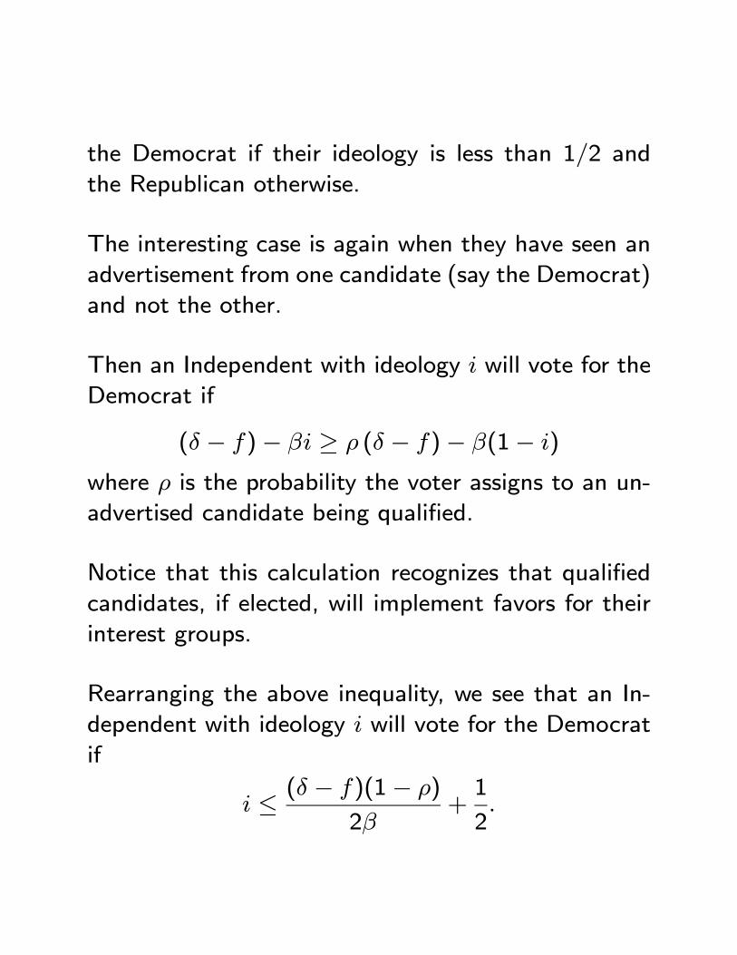
the Democrat if their ideology is less than 12 and

the Republican otherwise.

The interesting case is again when they have seen an

advertisement from one candidate (say the Democrat)

and not the other.

Then an Independent with ideology will vote for the

Democrat if

( − )− ≥ ( − )− (1− )

where is the probability the voter assigns to an un-

advertised candidate being qualified.

Notice that this calculation recognizes that qualified

candidates, if elected, will implement favors for their

interest groups.

Rearranging the above inequality, we see that an In-

dependent with ideology will vote for the Democrat

if

≤ ( − )(1− )

2+1

2

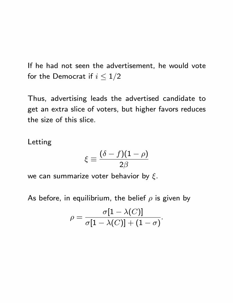
If he had not seen the advertisement, he would vote

for the Democrat if ≤ 12

Thus, advertising leads the advertised candidate to

get an extra slice of voters, but higher favors reduces

the size of this slice.

Letting

≡ ( − )(1− )

2

we can summarize voter behavior by .

As before, in equilibrium, the belief is given by

=[1− ()]

[1− ()] + (1− )

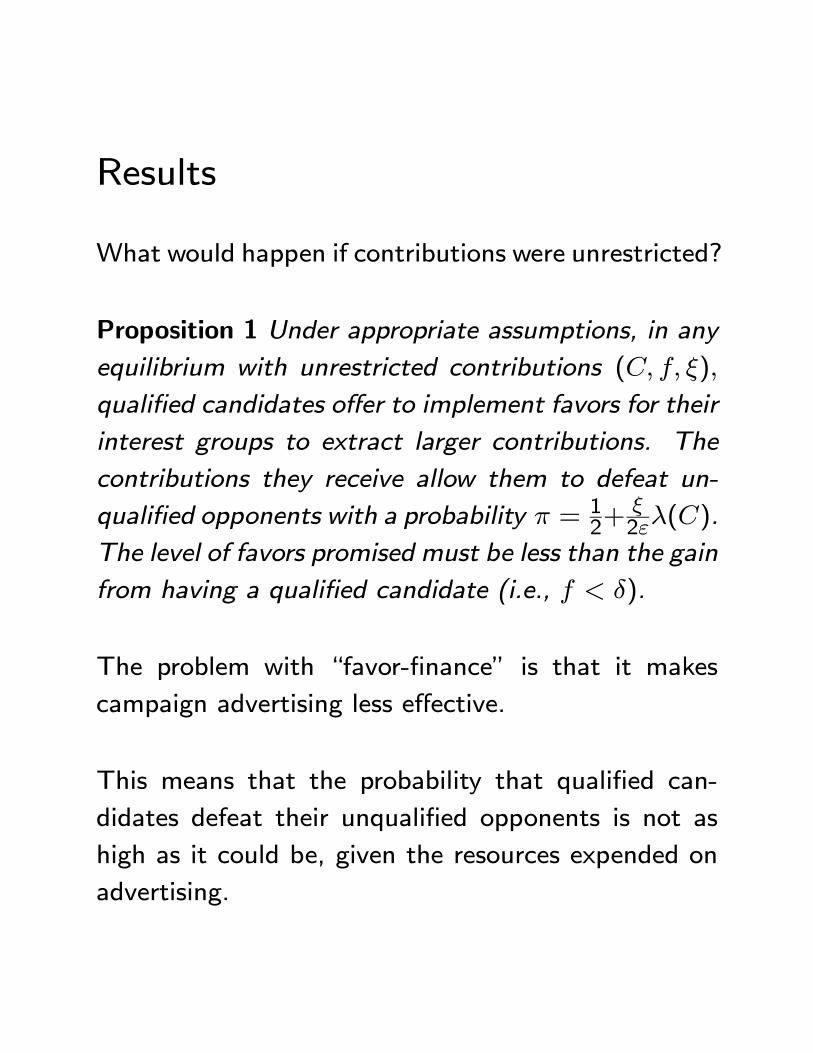
Results

What would happen if contributions were unrestricted?

Proposition 1 Under appropriate assumptions, in any

equilibrium with unrestricted contributions ( )

qualified candidates offer to implement favors for their

interest groups to extract larger contributions. The

contributions they receive allow them to defeat un-

qualified opponents with a probability = 12+ 2().

The level of favors promised must be less than the gain

from having a qualified candidate (i.e., ).

The problem with “favor-finance” is that it makes

campaign advertising less effective.

This means that the probability that qualified can-

didates defeat their unqualified opponents is not as

high as it could be, given the resources expended on

advertising.

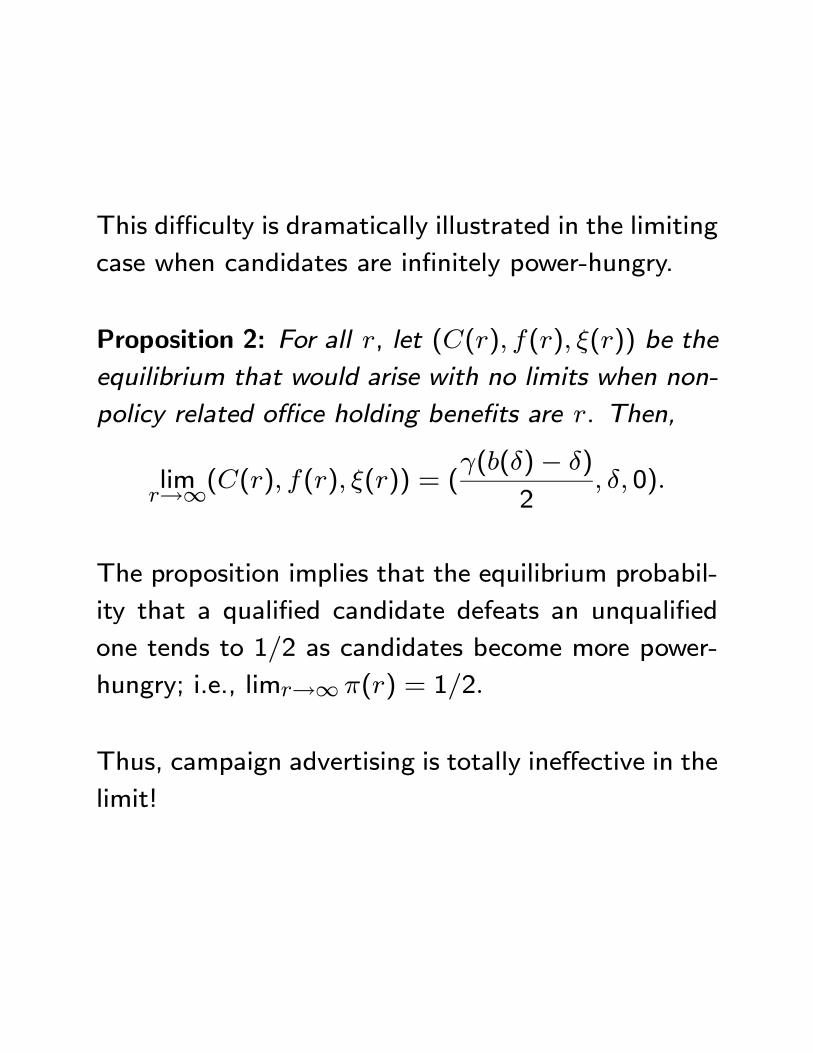
This difficulty is dramatically illustrated in the limiting

case when candidates are infinitely power-hungry.

Proposition 2: For all , let (() () ()) be the

equilibrium that would arise with no limits when non-

policy related office holding benefits are . Then,

lim→∞(() () ()) = (

(()− )

2 0)

The proposition implies that the equilibrium probabil-

ity that a qualified candidate defeats an unqualified

one tends to 12 as candidates become more power-

hungry; i.e., lim→∞ () = 12

Thus, campaign advertising is totally ineffective in the

limit!

Now lets introduce campaign finance policy.

Consider policies that impose a limit on the amount

an interest group can contribute and provide matching

public financing at rate (i.e., if a candidate raises

in private contributions he gets ).

Assume public financing is funded by a head tax .

Consider first what can be achieved with a pure con-

tribution limit policy ( = 0).

Fact If imposing a limit reduces the level of favors

and does not appreciably change the probability that

a qualified candidate defeats an unqualified one, then

it makes all types of citizens strictly better off.

The reason why interest groups are better off is that

all their gains from favors are paid for up front with

contributions.

Combining this result with Proposition 2 enables us

to establish:

Proposition 3 If candidates are sufficiently power-hungry

(i.e., is sufficiently large), banning contributions will

create a Pareto improvement.

Intuition: if contributions are banned entirely then

no favors will be promised and the probability that a

qualified candidate defeats an unqualified one is 12.

With less power-hungry candidates, banning contri-

butions could lead to a significant reduction in the

probability that qualified candidates defeat unquali-

fied ones.

However, limiting contributions need not appreciably

reduce the probability that qualified candidates win.

Limiting contributions reduces the level of favors and

this may increase advertising effectiveness.

This increase in effectiveness may compensate for the

reduction in the level of advertising.

Unfortunately, while all this is possible, it is difficult

to find sufficient conditions under which there exists

a Pareto improving limit.

With public financing, public funds can substitute for

the reduction in spending caused by limits.

Proposition 4 Suppose that the Assumptions of Propo-

sition 1 are satisfied and let (∗ ∗ ∗) be an equi-librium with unrestricted contributions. Then there

exists a campaign finance policy ( ) and an equilib-

rium ( ) under ( ) such that ( ) Pareto

dominates (∗ ∗ ∗).

Thus, there always exists a Pareto improving cam-

paign finance policy!

It is interesting to note that the campaign finance poli-

cies that the model suggests can be Pareto improv-

ing, closely resemble the Clean Money, Clean Elections

program discussed earlier.

Indirectly informative advertising

The above model assumes that advertising directly

informs voters of candidate characteristics.

Another branch of literature looks at indirectly infor-

mative advertising.

According to this perspective, it is the fact that a can-

didate has been given contributions that is the signal

- not the messages per se.

When advertising is indirectly informative, banning

contributions may improve aggregate voter welfare as

shown by Prat (2003).

Basic trade off is between losses of information and

benefits from reduced policy distortion.

However, the indirectly informative view does not ap-

pear to support public financing or contribution limits.

In many respects, neither the directly or the indirectly

informative advertising models are very satisfactory.

There is a need for a better model of advertising in-

corporating the idea of persuasion - see DellaVigna

and Gentzkow (2010) for more discussion.

Other relevant work

Houser and Stratmann (2008) study experimentally a

game based on Coate (2004).

They provide experimental evidence for the idea that

campaign advertising financed by favors is less effec-

tive than advertising financed by clean money.

Ashworth (2006) develops a model very similar to

Coate (2004), but relaxes the assumption of candi-

date symmetry.

He notes that incumbent candidates have their ad-

vantage reinforced because challengers must promise

more favors to get money for campaigning since they

are less likely to be elected.

This means that challenger advertising is less effective

and helps explain the extent of incumbent bias.

Vanberg (2008) explores theoretically and empirically

a different argument for campaign contribution limits

- the equalization argument.

The argument is that contribution limits are desirable

because they equalize the influence of different donors

and therefore cause a candidate’s campaign resources

to better reflect his public support.

Vanberg uses a theoretical model to identify the as-

sumptions under which this argument makes sense

and then analyzes whether these assumptions are sat-

isfied empirically.

Prat, Puglisi, and Snyder (2010) study the extent to

which private campaign contributions are targeted to

better candidates.

They are interested in analyzing the common critique

of public funding that funds allocated publicly will not

get to the right candidates.

This critique is dealt with in practice in the Clean

Money schemes by giving public money only to candi-

dates with the required number of small contributions.

Prat, Puglisi, and Snyder provide some support for

this practice by showing that the sum of small contri-

butions (as opposed to the total sum of contributions)

is strongly correlated with legislator effectiveness.

IV.4 Fiscal Policy and FiscalRestraints

In public choice theory it is common to distinguish

between the political and the fiscal constitution.

The political constitution specifies the electoral rules

which govern how representatives are elected.

The fiscal constitution constrains the policies repre-

sentatives may choose.

For example, the fiscal constitution could require that

representatives run a balanced budget; that revenue

by raised only from property taxes; that taxes cannot

be person-specific; etc.

The fiscal constitution might also specify procedures

by which fiscal decisions must be made; for example,

raising taxes requires a super-majority vote in the leg-

islature.

The idea of a fiscal constitution is to appropriately

constrain politicians’ fiscal choices and reflects politi-

cal economy concerns.

Obviously, if government were benevolent no such

constraints would be desirable.

In the public choice literature, the case for having a

fiscal constitution has been made by James Buchanan

and his co-authors.

Buchanan has also written a number of papers ana-

lyzing what principles should guide the choice of fiscal

constitution.

Brennan and Buchanan (1977) is the best known ex-

ample.

Brennan and Buchanan

This paper employs a very simple model of govern-

ment - the so-called Leviathan model.

According to this model, the government sets taxes

to maximize revenue.

It spends a fixed fraction of this revenue on public

goods and services and the remainder is wasted (the

idea is that the government consumes it somehow in

unproductive ways).

The question addressed by Brennan and Buchanan, is

that if this is the right model of government, what

should it be allowed to tax?

The key problem is to allow the government to raise

sufficient revenue as to provide valued public goods

and services, but to not allow it to extract too much

revenue.

The main point made by Brennan and Buchanan is

that all the lessons of traditional public finance are

turned on their head.

For example, taxing goods that are in inelastic demand

is recommended by optimal tax theory because this

minimizes distortions.

But allowing a Leviathan government to tax a good in

inelastic demand would be a disaster - it would raise

too much revenue.

Similarly, while traditional public finance recommends

government have a comprehensive tax base (i.e., in-

come, commodity, wealth, etc) to minimize distor-

tions, a narrow base (e.g., only income) is desirable

with a Leviathan government.

Subsequent literature

The subsequent literature on fiscal restraints has two

strands.

One strand is devoted to the empirical question of

whether the fiscal restraints that are used in practice

actually have any effect.

For example, Poterba (1996) discusses the impact of

balanced budget rules which are common at the state

level in the U.S..

The key question is whether legislators can circumvent

these rules via accounting gimmicks and the like.

The literature tends to finds that rules do matter:

Poterba shows that states with more stringent re-

straints are quicker to reduce spending and/or raise

taxes in response to negative revenue shocks than

those without.

Knight (2000) looks at the impact of supermajority

requirement for tax increases which are found in some

states.

He argues that such requirements have significantly

reduced taxes.

The second strand of work is devoted to the basic the-

oretical question of whether, assuming that they can

be enforced and will not be circumvented, particular

fiscal restraints are desirable.

Besley and Smart (2007) provide an analysis of bal-

anced budget rules and other fiscal restraints in the

context of a two period political agency model.

The key issue in their analysis is how having fiscal

restraints influences the flow of information to citizens

concerning the characteristics of their politicians.

Azzimonti, Battaglini, and Coate (2008) provide a

theoretical analysis of the case for a balanced budget

rule in the context of Battaglini and Coate’s (2008)

political economy model of fiscal policy.

They also calibrate the model to the U.S. economy

to assess the case for a balanced budget rule for the

federal government.

This is motivated by the recurring debate in Amer-

ican politics concerning the desirability of amending

the U.S. constitution to require that the federal gov-

ernment operate under such a rule.

We will review this analysis, beginning with a review

of the Battaglini and Coate model.

Battaglini and Coate model

This combines a “tax smoothing model” of fiscal pol-

icy with a legislative bargaining model of policy deter-

mination.

It incorporates the friction that legislators can distrib-

ute pork back to their districts and analyzes how this

distorts fiscal policy.

The key contribution is to shed light on how a stan-

dard feature of legislative policy-making (pork-barrel

politics) distorts macro fiscal policies.

The economy

A continuum of infinitely-lived citizens live in iden-

tical districts indexed by = 1 .

The size of the population in each district is normal-

ized to be one.

There is a single (nonstorable) consumption good, de-

noted by , that is produced using a single factor, la-

bor, denoted by , with the linear technology = .

There is also a public good, denoted by , that can

be produced from the consumption good according to

the technology = .

Consumers consume the consumption good, benefit

from the public good, and supply labor.

Each consumer’s per period utility function is

+ − (1+1)(1 + )

where ∈ (0 1) and 0.

The parameter measures the value of the public

good.

Citizens discount future per period utilities at rate .

The value of the public good varies across periods in

a random way, reflecting shocks to the society such

as wars and natural disasters.

Specifically, in each period, is the realization of a

random variable with range [0 1] (where 0 0

1) and cumulative distribution function ().

There is a competitive labor market and competitive

production of the public good.

Thus, the wage rate is equal to and the price of the

public good is .

There is also a market in risk-free one period bonds.

The assumption of a constant marginal utility of con-

sumption implies that the equilibrium interest rate on

these bonds must be = 1 − 1.

At this interest rate, consumers will be indifferent as

to their allocation of consumption across time.

Government

The public good is provided by the government.

The government can raise revenue by levying a pro-

portional tax on labor income.

It can also borrow and lend in the bond market by

selling and buying bonds.

Revenues can not only be used to finance the provision

of the public good but can also be used to finance

a district specific transfers (non-distortionary “pork-

barrel” spending).

At the beginning of each period, the government in-

herits a level of public debt from the previous gov-

ernment.

This must be repaid with interest, which costs (1+).

Government policy in the period is described by a +

3-tuple

{ 0 1 }where is the income tax rate; is the amount of the

public good provided; 0 is the proposed new level ofpublic debt; and is the proposed transfer to district

’s residents.

When 0 is negative, the government is buying bonds.

In a period in which government policy is { 0 1 },each consumer will supply an amount of labor

∗((1− )) = argmax{(1− )− (1+1)

+ 1}

It is straightforward to show that ∗((1 − )) =

((1−)), so that is the elasticity of labor supply.

A consumer who simply consumes his net of tax earn-

ings and his transfer will obtains a per period utility

of ((1− ) ;) + where

((1− ) ;) =((1− ))+1

+ 1+

Since consumers are indifferent as to their allocation

of consumption across time, their lifetime expected

utility will equal that which they would obtain if they

simply consumed their net earnings and transfer each

period plus the value of their initial bond holdings.

Feasibility constraints

Government policies must satisfy three feasibility con-

straints.

The first is that revenues must be sufficient to cover

expenditures.

To see what this implies, consider a period in which

the initial level of government debt is and the policy

choice is { 0 1 }

Expenditure on public goods and debt repayment is

+ (1 + ).

Tax revenues are

() = ∗((1− )) = ((1− ))

and total revenues are () + 0.

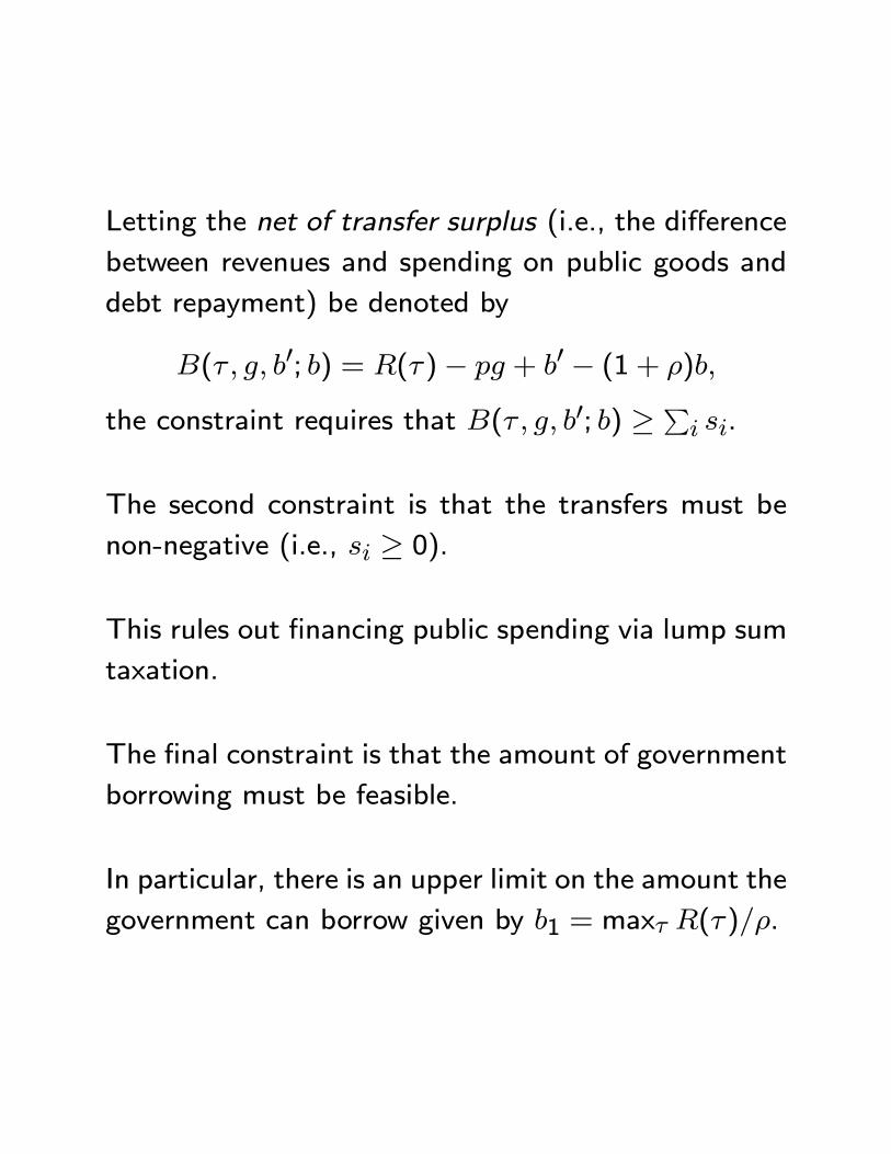
Letting the net of transfer surplus (i.e., the difference

between revenues and spending on public goods and

debt repayment) be denoted by

( 0; ) = ()− + 0 − (1 + )

the constraint requires that ( 0; ) ≥ P .

The second constraint is that the transfers must be

non-negative (i.e., ≥ 0).

This rules out financing public spending via lump sum

taxation.

The final constraint is that the amount of government

borrowing must be feasible.

In particular, there is an upper limit on the amount the

government can borrow given by 1 = max ().

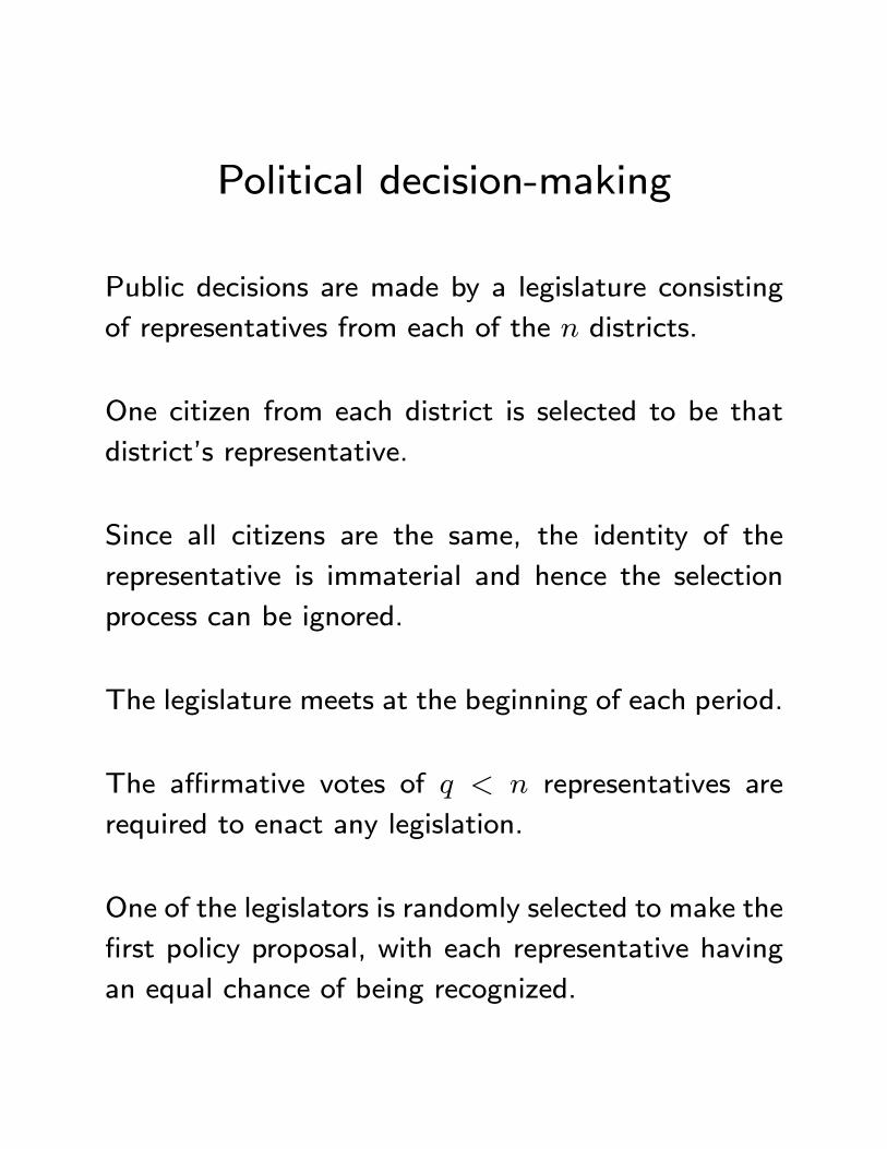
Political decision-making

Public decisions are made by a legislature consisting

of representatives from each of the districts.

One citizen from each district is selected to be that

district’s representative.

Since all citizens are the same, the identity of the

representative is immaterial and hence the selection

process can be ignored.

The legislature meets at the beginning of each period.

The affirmative votes of representatives are

required to enact any legislation.

One of the legislators is randomly selected to make the

first policy proposal, with each representative having

an equal chance of being recognized.

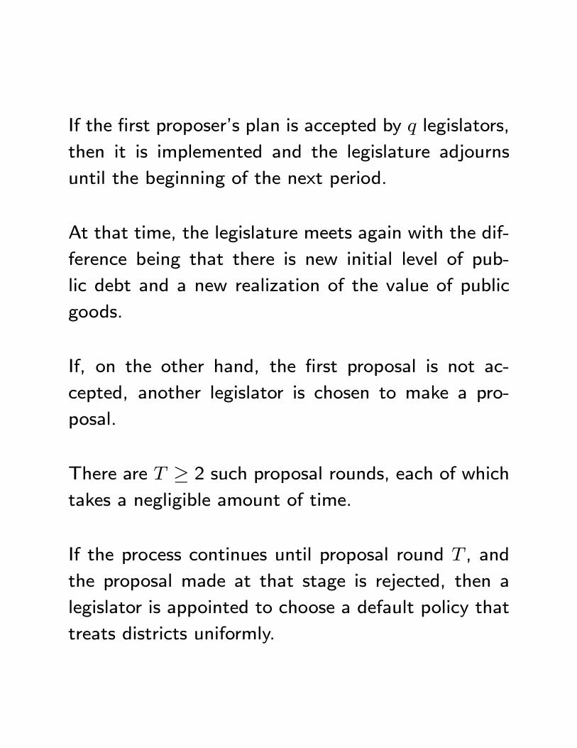
If the first proposer’s plan is accepted by legislators,

then it is implemented and the legislature adjourns

until the beginning of the next period.

At that time, the legislature meets again with the dif-

ference being that there is new initial level of pub-

lic debt and a new realization of the value of public

goods.

If, on the other hand, the first proposal is not ac-

cepted, another legislator is chosen to make a pro-

posal.

There are ≥ 2 such proposal rounds, each of whichtakes a negligible amount of time.

If the process continues until proposal round , and

the proposal made at that stage is rejected, then a

legislator is appointed to choose a default policy that

treats districts uniformly.

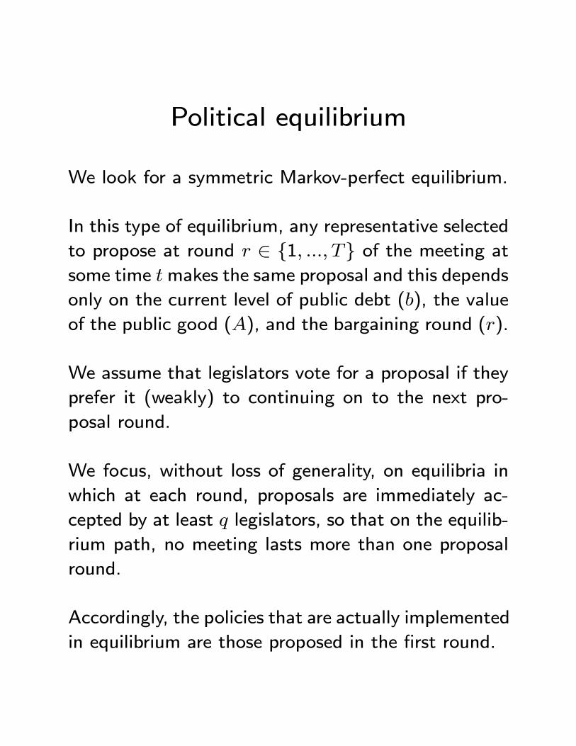
Political equilibrium

We look for a symmetric Markov-perfect equilibrium.

In this type of equilibrium, any representative selected

to propose at round ∈ {1 } of the meeting atsome time makes the same proposal and this depends

only on the current level of public debt (), the value

of the public good (), and the bargaining round ().

We assume that legislators vote for a proposal if they

prefer it (weakly) to continuing on to the next pro-

posal round.

We focus, without loss of generality, on equilibria in

which at each round, proposals are immediately ac-

cepted by at least legislators, so that on the equilib-

rium path, no meeting lasts more than one proposal

round.

Accordingly, the policies that are actually implemented

in equilibrium are those proposed in the first round.

Equilibrium policies

To understand equilibrium behavior note that to get

support for his proposal, the proposer must obtain the

votes of − 1 other representatives.

Given that utility is transferable, the proposer is ef-

fectively making decisions to maximize the utility of

legislators.

It is therefore as if a randomly chosen minimum win-

ning coalition (mwc) of representatives is selected in

each period and this coalition chooses a policy choice

to maximize its aggregate utility.

In any given state (), there are two possibilities:

either the mwc will provide pork to the districts of its

members or it will not.

Providing pork requires reducing public good spending

or increasing taxation in the present or the future (if

financed by issuing additional debt).

When and/or are sufficiently high, the marginal

benefit of spending on the public good and the mar-

ginal cost of increasing taxation may be too high to

make this attractive.

In this case, the mwc will not provide pork and the

outcome will be as if it is maximizing the utility of

the legislature as a whole.

If the mwc does provide pork, it will choose a tax rate-

public good-public debt triple that maximizes coalition

aggregate utility under the assumption that they share

the net of transfer surplus.

Thus, ( 0) solves the problem:

max((1− ) ;) +(0;)

+ (0 0)

0 ≤ 1

where is the continuation value function.

The optimal policy is (∗ ∗() ∗) where the taxrate ∗ satisfies the condition that

1

=[ 1−∗1−∗(1+)]

the public good level ∗() satisfies the condition that

∗()−1 =

and the public debt level ∗ satisfies

1

= −[(

∗ 0)0

]

The first condition says that the benefit of raising

taxes in terms of increasing the per-coalition member

transfer (1) must equal the per-capita cost of the

increase in the tax rate.

The second condition says that the per-capita bene-

fit of increasing the public good must equal the per-

coalition member reduction in transfers it necessitates.

The third condition says that the benefit of increasing

debt in terms of increasing the per-coalition member

transfer must equal the per-capita cost of an increase

in the debt level.

The mwc will choose pork if the net of transfer surplus

at the optimal policy (∗ ∗() ∗; ) is positive.

Otherwise the coalition will provide no pork and its

policy choice will then maximize aggregate legislator

(and hence citizen) utility.

In this case, the tax rate will exceed ∗, the publicgood level will be less than ∗(), and the publicdebt level will exceed ∗.

The following result explains how the temptation to

distribute pork distorts the political equilibrium:

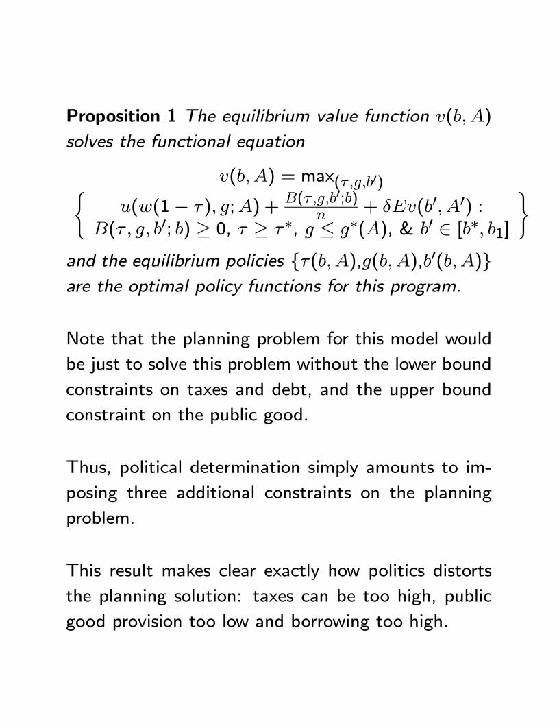
Proposition 1 The equilibrium value function ()

solves the functional equation

() = max(0)(((1− ) ;) +

(0;)

+ (0 0) :( 0; ) ≥ 0, ≥ ∗, ≤ ∗(), & 0 ∈ [∗ 1]

)and the equilibrium policies {(),(),0()}are the optimal policy functions for this program.

Note that the planning problem for this model would

be just to solve this problem without the lower bound

constraints on taxes and debt, and the upper bound

constraint on the public good.

Thus, political determination simply amounts to im-

posing three additional constraints on the planning

problem.

This result makes clear exactly how politics distorts

the planning solution: taxes can be too high, public

good provision too low and borrowing too high.

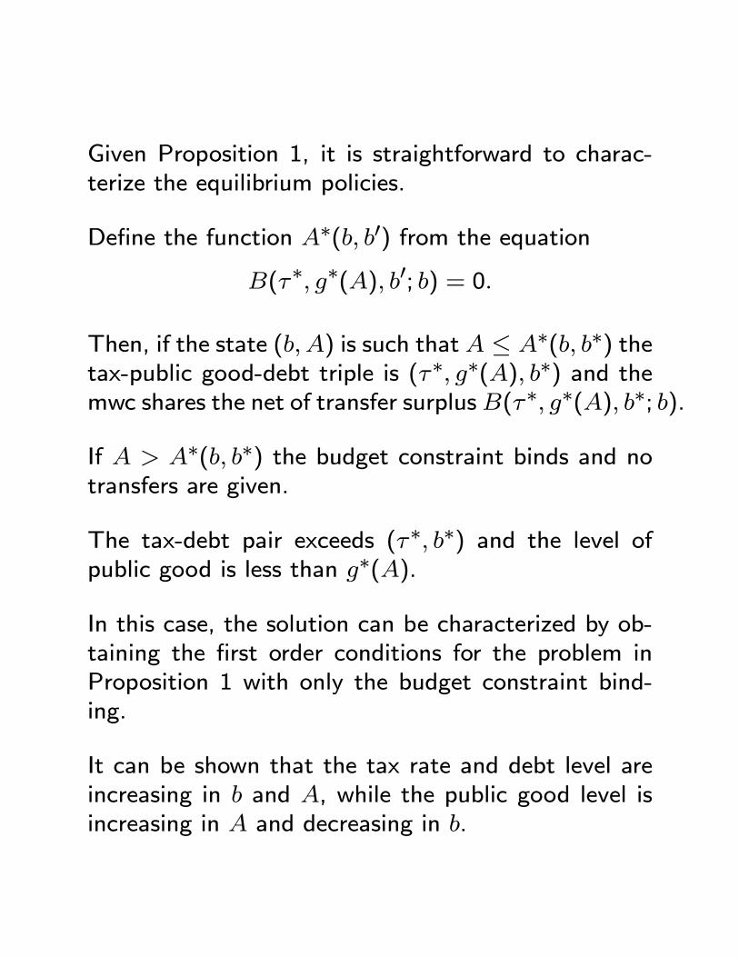
Given Proposition 1, it is straightforward to charac-

terize the equilibrium policies.

Define the function ∗( 0) from the equation

(∗ ∗() 0; ) = 0

Then, if the state () is such that ≤ ∗( ∗) thetax-public good-debt triple is (∗ ∗() ∗) and themwc shares the net of transfer surplus(∗ ∗() ∗; ).

If ∗( ∗) the budget constraint binds and notransfers are given.

The tax-debt pair exceeds (∗ ∗) and the level ofpublic good is less than ∗().

In this case, the solution can be characterized by ob-

taining the first order conditions for the problem in

Proposition 1 with only the budget constraint bind-

ing.

It can be shown that the tax rate and debt level are

increasing in and , while the public good level is

increasing in and decreasing in .

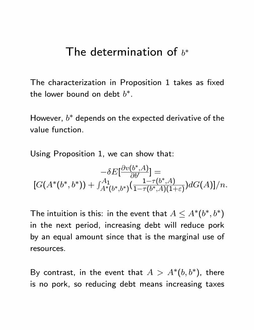
The determination of ∗

The characterization in Proposition 1 takes as fixed

the lower bound on debt ∗.

However, ∗ depends on the expected derivative of thevalue function.

Using Proposition 1, we can show that:

−[(∗)0 ] =

[(∗(∗ ∗)) +R1∗(∗∗)(

1−(∗)1−(∗)(1+))()]

The intuition is this: in the event that ≤ ∗(∗ ∗)in the next period, increasing debt will reduce pork

by an equal amount since that is the marginal use of

resources.

By contrast, in the event that ∗( ∗), thereis no pork, so reducing debt means increasing taxes

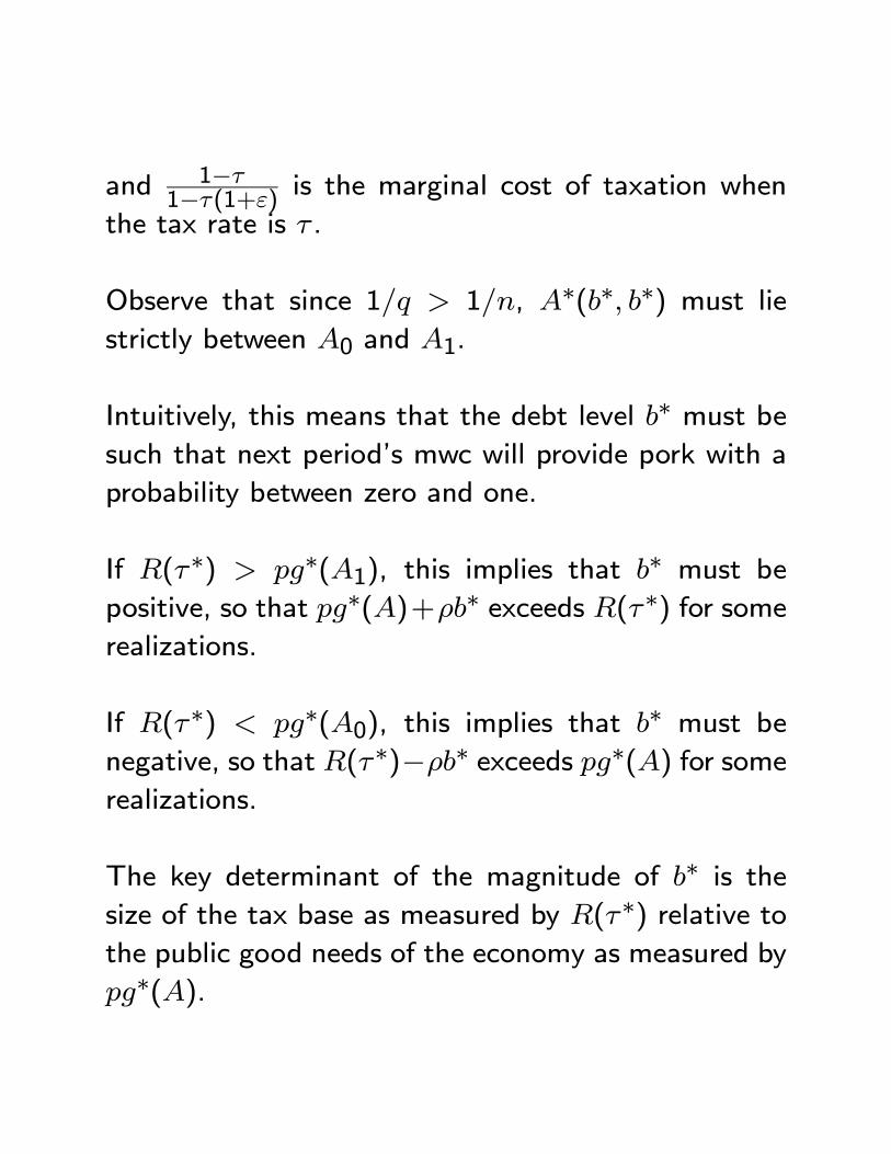
and 1−1−(1+) is the marginal cost of taxation when

the tax rate is .

Observe that since 1 1, ∗(∗ ∗) must liestrictly between 0 and 1.

Intuitively, this means that the debt level ∗ must besuch that next period’s mwc will provide pork with a

probability between zero and one.

If (∗) ∗(1), this implies that ∗ must bepositive, so that ∗()+∗ exceeds (∗) for somerealizations.

If (∗) ∗(0), this implies that ∗ must benegative, so that (∗)−∗ exceeds ∗() for somerealizations.

The key determinant of the magnitude of ∗ is thesize of the tax base as measured by (∗) relative tothe public good needs of the economy as measured by

∗().

Equilibrium dynamics

The long run behavior of fiscal policies in the political

equilibrium is summarized in the following proposition:

Proposition 2 The equilibrium debt distribution con-

verges to a unique, non-degenerate invariant distribu-

tion whose support is a subset of [∗ 1]. When thedebt level is ∗, the tax rate is ∗, the public goodlevel is ∗(), and a minimum winning coalition of

districts receive pork. When the debt level exceeds

∗, the tax rate exceeds ∗, the public good level isless than ∗(), and no districts receive pork.

Thus equilibrium fiscal policies fluctuate in the long

run in response to shocks in the value of the public

good.

Legislative policy-making oscillates between periods of

pork-barrel spending and periods of fiscal responsibil-

ity.

Periods of pork are brought to an end by high realiza-

tions in the value of the public good.

These trigger an increase in debt and taxes to finance

higher public good spending and a cessation of pork.

Once in the regime of fiscal responsibility, further high

realizations of trigger further increases in debt and

higher taxes.

Pork returns only after a suitable sequence of low re-

alizations of .

The larger the amount of debt that has been built up,

the greater the expected time before pork re-emerges.

It is worth comparing this long run behavior with that

arising under the planning solution.

In the planning solution, the government gradually

builds up sufficient assets to finance the Samuelson

level of the public good in each period with no taxa-

tion.

Azzimonti, Battaglini, and Coate

Azzimonti et al address the following question: what

would happen if, once debt was at long run equilibrium

levels (i.e., ∈ [∗ 1]), a balanced budget rule wereto be imposed on the economy?

They model a balanced budget rule as a requirement

that tax revenues must always be sufficient to cover

spending and the costs of servicing the debt.

If the initial level of debt is , this requires that

() ≥ +X

+

Given the definition of ( 0; ), such a rule isequivalent to adding, in each period, the feasibility

constraint that 0 ≤ ; i.e., that debt cannot increase.

Thus, under a balanced budget rule, next period’s fea-

sible debt levels are determined by this period’s debt

choice.

In particular, if debt is paid down in the current period,

that will tighten the debt constraint in the next period.

To state the main result of their paper, let (() ())

be the tax rate and public good level that solve the

static maximization problem

max()

(((1− ) ;) +

( )

: ( ) ≥ 0

)

Proposition 3 Suppose that a balanced budget rule

is imposed on the economy when the debt level is in

the range [∗ 1). Then, debt will converge monoton-ically to a steady state level 0 smaller than ∗. Atthis steady state level 0, when the value of the public

good is less than ∗(0 0), the tax rate will be ∗,the public good level will be ∗(), and a mwc of dis-tricts will receive pork. When the value of the public

good is greater than ∗(0 0), the tax rate will be0(), the public good level will be 0(), and no

districts will receive pork.

The intuition behind the debt reduction is that a bal-

anced budget rule, by restricting future policies, in-

creases the expected cost of taxation and increases

legislators’ incentive to save.

The above proposition provides a reasonably complete

picture of how imposing a balanced budget rule will

impact fiscal policy.

However, Azzimonti et al are also interested in the

impact on citizens’ welfare.

The argue that when the rule is first imposed, it will

reduce contemporaneous utility.

When is low, instead of transfers being paid out to

the citizens, debt will be being paid down.

When is high, the increase in taxes and reduction

in public goods will be steeper than would be the case

if the government could borrow.

Thus, in either case, citizen welfare will be lower.

As debt falls, the picture becomes less clear.

On the one hand, citizens gain from the higher aver-

age public spending levels and/or lower taxes resulting

from the smaller debt service payments.

On the other hand, public good provision will be less

responsive and there will be greater volatility in tax

rates.

The inability to run deficits means that the only way

to respond to positive shocks in the value of the public

good is to raise taxes.

This leads to sharper tax hikes and, since the marginal

cost of public funds is higher, public good provision

incentives are dampened.

Thus, there is a clear trade-off whose resolution will

depend on the parameters.

In their calibrated model, long run welfare is actually

increased by 2.85%.

However, when account is taken of the short run tran-

sition costs, imposing a balanced budget rule reduces

welfare.

Discussion

The balanced budget rule studied by Azzimonti et al

differs from the rules actually proposed in Congress.

In particular, these rules can be overrided with a super-

majority vote.

Azzimonti et al show that imposing a balanced budget

rule with a super-majority override will have no effect

on fiscal policy or citizen welfare.

Such a rule will only have an effect if imposed at the

foundation of the state before debt has risen to equi-

librium levels.

Intuitively, this is because in the Battaglini and Coate

model, once debt has reached equilibrium levels, addi-

tional debt will be issued only when it is in the interests

of all legislators to do so, rather than just a minimum

winning coalition.

This result reflects the stationarity of the Battaglini

and Coate model and would not necessarily apply in

a growing economy.

Another feature of the rules actually proposed is that

they are automatically suspended in times of war.

If we interpret war as periods in which is high, hav-

ing such an automatic suspension rule may be helpful

in reducing the costs of a balanced budget rule.

This has yet to be studied.

There is plenty of scope for much more analysis of

fiscal restraints in this style (see Bassetto and Sargent

(2006) for another example).

IV.7 Electing the President

The president of the U.S. is probably the world’s most

powerful leader.

The president is elected by a very distinctive process

which happens every four years.

At the beginning of an election year, there are presi-

dential primaries which consist of sequential statewide

contests that run from January through June.

The first contests are traditionally in Iowa, New Hamp-

shire, and South Carolina.

These primaries are designed to pick the two parties’

nominees who are annointed at the parties’ national

conventions which are held in the late summer.

Over the late summer and early fall, the two nominees

campaign for the national election which is held in the

first week of November.

The November election is not decided by a direct na-

tional vote but by the Electoral College system.

In this system, each state is represented by a slate

of “electors” the number of which equals the state’s

number of senators (i.e., 2) plus the number of its

House representatives.

The electors then cast their votes on behalf of their

state and the candidate with the most votes wins.

By convention, the electors of all states except Maine

and Nebraska cast their vote in favor of the candidate

who wins a majority of votes in their state.

In Maine and Nebraska, two electoral votes are deter-

mined by the statewide vote, and the remainder by

the votes in each congressional district.

Two recent papers study some of the anomalies cre-

ated by this system.

Knight and Schiff (2010) focus on the idea that the

sequential nature of the primary system gives voters

in the early states more weight in determining the

outcome.

This is a very common complaint about the system.

Stromberg (2008) focuses on the incentives created by

the Electoral College in terms of which states receive

attention during the campaign.

Both papers are very good and represent examples

of frontier research in political economy combining

theory and empirics.

We will discuss only the Stromberg paper because of

time constraints.

Stromberg’s Paper

Stromberg is interested in the long-standing argument

that the Electoral College creates incentives for presi-

dential candidates to only pay attention to a handful

of key swing states.

To empirically measure the power of these incentives,

he focuses on the allocation of presidential and vice-

presidential visits during the campaign period follow-

ing the two parties’ nominating conventions.

He develops a model of campaign visits based on the

Lindbeck-Weibull model and studies it’s performance

empirically.

He then uses the model to compare the equilibrium

allocation of campaign visits with that which would

arise if the president were elected by a direct national

vote.

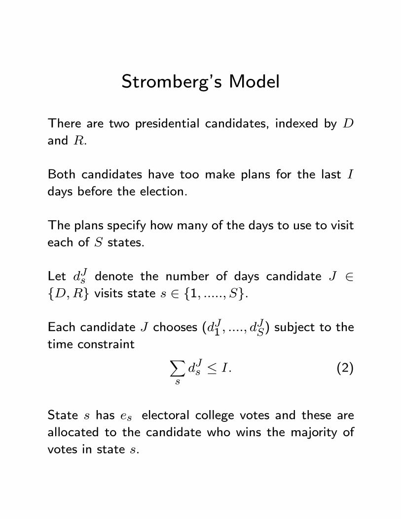
Stromberg’s Model

There are two presidential candidates, indexed by

and .

Both candidates have too make plans for the last

days before the election.

The plans specify how many of the days to use to visit

each of states.

Let denote the number of days candidate ∈{} visits state ∈ {1 }.

Each candidate chooses (1 ) subject to the

time constraint X ≤ . (2)

State has electoral college votes and these are

allocated to the candidate who wins the majority of

votes in state .

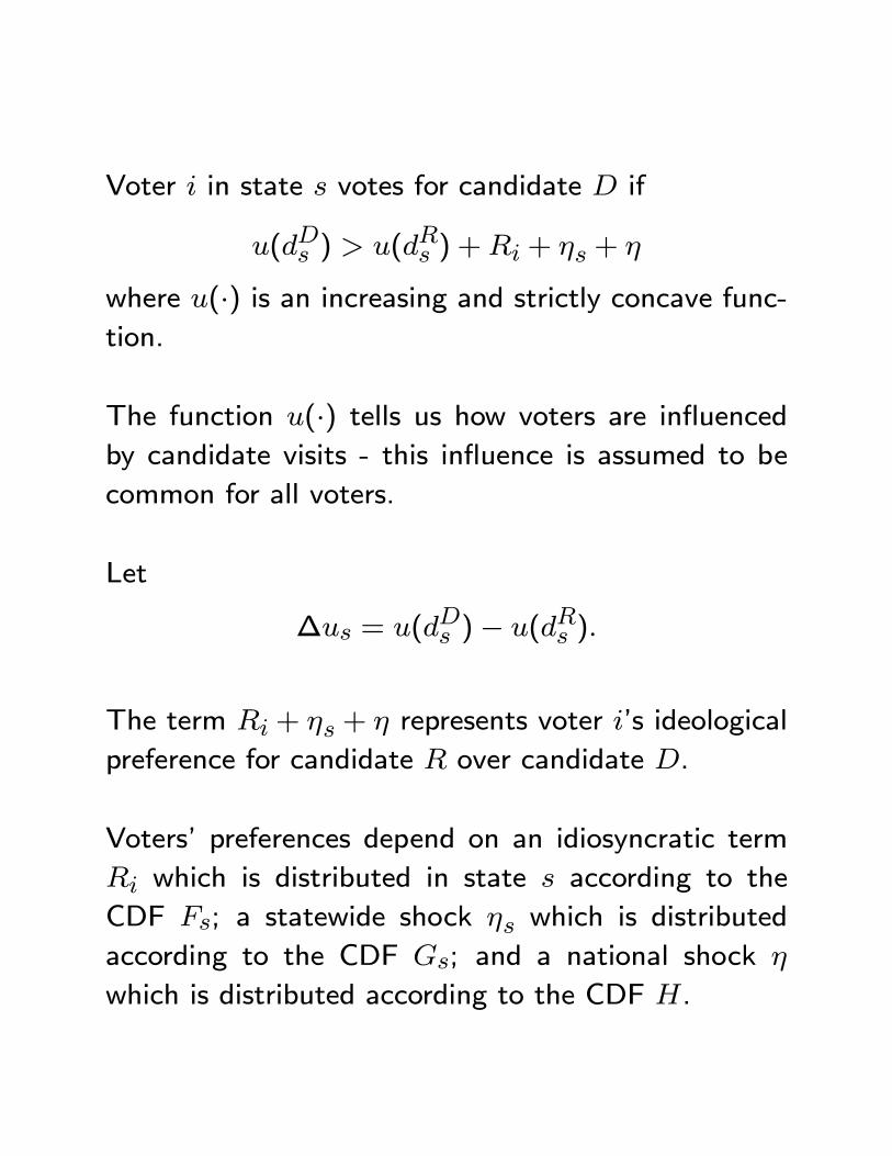
Voter in state votes for candidate if

( ) ( ) + + +

where (·) is an increasing and strictly concave func-tion.

The function (·) tells us how voters are influenced

by candidate visits - this influence is assumed to be

common for all voters.

Let

∆ = ( )− ( )

The term + + represents voter ’s ideological

preference for candidate over candidate .

Voters’ preferences depend on an idiosyncratic term

which is distributed in state according to the

CDF ; a statewide shock which is distributed

according to the CDF ; and a national shock

which is distributed according to the CDF .

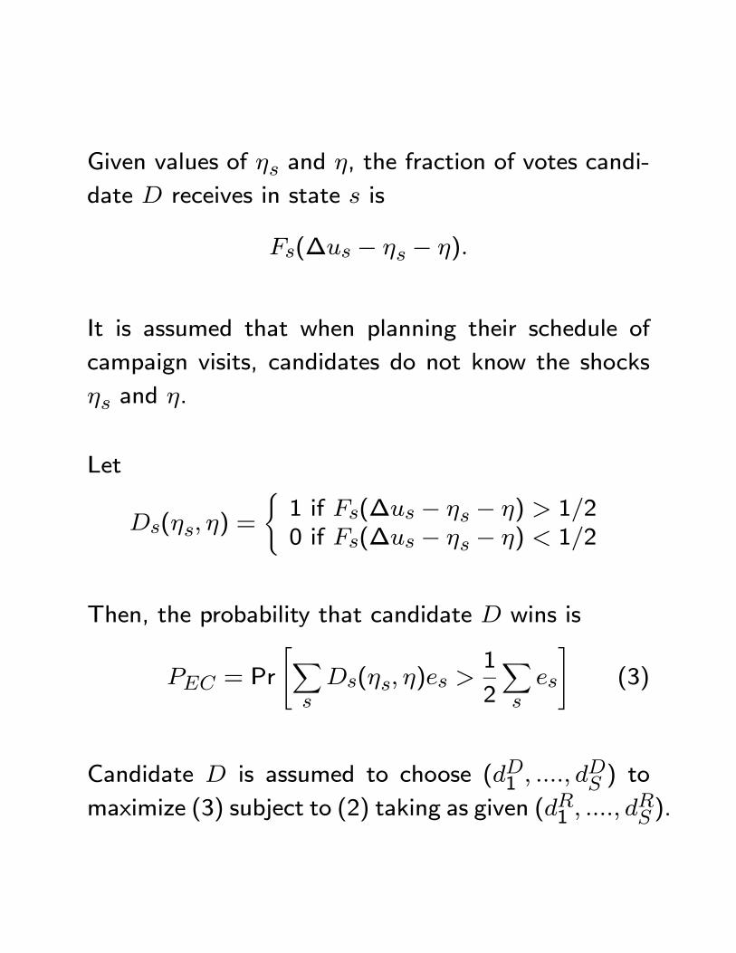
Given values of and , the fraction of votes candi-

date receives in state is

(∆ − − )

It is assumed that when planning their schedule of

campaign visits, candidates do not know the shocks

and .

Let

( ) =

(1 if (∆ − − ) 12

0 if (∆ − − ) 12

Then, the probability that candidate wins is

= Pr

"X( )

1

2

X

#(3)

Candidate is assumed to choose (1 ) to

maximize (3) subject to (2) taking as given (1 ).

Candidate is assumed to choose (1 ) to

minimize (3) subject to (2) taking as given (1 ).

Actually maximizing or minimizing (3) is complicated,

so Stromberg comes up with a clever way to approxi-

mate (3).

He also chooses parametrized functional forms for the

CDFs which allow him to solve for the equilibrium in

closed form as a function of the parameters.

In equilibrium, the two candidates will choose identical

schedules of campaign visits, following the logic of the

Lindbeck- Weibull model.

Stromberg then estimates the parameters of the CDFs

using past voting data, polls, etc and obtains his equi-

librium predictions.

Figure 1 of his paper compares the predictions of

his model with data on actual presidential and vice-

presidential visits from the 2000 and 2004 campaigns.

The estimates are pretty close to the actual visits.

Direct Vote vs Electoral College

Let the number of voters in state be denoted .

Then, with a direct national vote, the probability that

candidate wins is

= Pr

"X(∆ − − )

1

2

X

#(4)

How would the allocation of campaign visits compare

under the two systems?

Figure 6 of his paper deals with this question.

States above 1 on the vertical axis receive more than

average visits per capita under the Electoral College

system.

States above 1 on the horizontal axis receive more

than average visits per capita with a Direct Vote.

States above the 45 line lose from the reform and

states below gain.

States gain or lose attention because of (i) their elec-

toral size per capita and (ii) influence relative to elec-

toral size.

States like RI and MA gain under Direct Vote because,

while their average partisanship is high, they do have

quite a lot of swing voters.

Their high average partisanship means that they are

rarely competitive and thus attract little attention un-

der the Electoral College.

Their large fraction of swing voters make them attrac-

tive targets under the Direct Vote.

States like NV and DE lose because they have a heavy

endowment of electoral votes relative to popular votes

(i.e., high relative to ).

In terms of the aggregate distribution, equilibrium vis-

its are much more concentrated under the Electoral

College than the Direct Vote.

IV.8 Federalism

In many countries, there are different levels of govern-

ment.

In the U.S., for example, we have the federal govern-

ment, state governments, and local governments.

A classic question in public choice concerns the ap-

propriate allocation of policy responsibility to the dif-

ferent government levels.

What policies should the various levels of government

be responsible for?

We will review a number of arguments that are rele-

vant for thinking about this question.

IV.8.i Spillovers vs Preference Hetero-geneity

Wallace Oates in his classic book Fiscal Federalism

presented an influential way of thinking about the as-

signment of policy responsibility between national and

local governments.

Assignment of policy responsibility to the local level

was desirable if there was significant preference het-

erogeneity between localities and if there were limited

policy spillovers across localities.

To see the argument, consider the following model.

An economy is divided into two geographically distinct

districts indexed by ∈ {1 2}.

Each district has a continuum of citizens with a mass

of unity.

There are three goods in the economy; a single private

good, , and two local public goods, 1 and 2, each

one associated with a particular district.

These local public goods could be thought of as roads

or parks.

Each citizen is endowed with some of the private good.

To produce one unit of either of the public goods,

requires units of the private good.

Each citizen in district is characterized by a public

good preference parameter .

The preferences of a type citizen in district are

+ [(1− ) ln + ln −]

The parameter ∈ [0 12] indexes the degree of

spillovers.

When = 0 citizens care only about the public good

in their own district, while when = 12 they care

equally about the public goods in both districts.

The mean type in district is denoted by , where

1 ≥ 2.

We are interested in whether responsibility for choos-

ing the local public goods should be assigned to local

or national governments.

With local provision, the level of public good in each

district is chosen by the government of that district

and public expenditures are financed by a uniform

head tax on local residents.

Thus, if district chooses a public good level , each

citizen in district pays a tax of .

With national provision, a uniform public good level is

chosen by a national government with spending being

financed by a uniform head tax on all citizens.

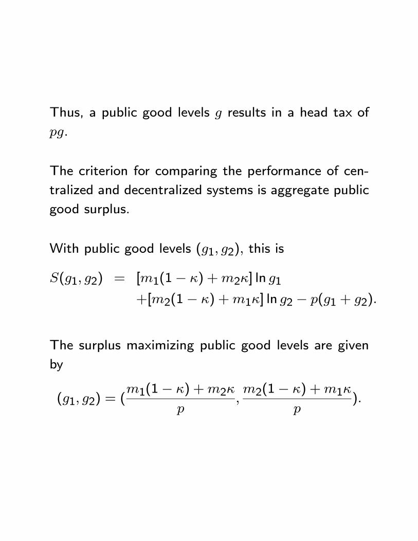
Thus, a public good levels results in a head tax of

.

The criterion for comparing the performance of cen-

tralized and decentralized systems is aggregate public

good surplus.

With public good levels (1 2) this is

(1 2) = [1(1− ) +2] ln 1

+[2(1− ) +1] ln 2 − (1 + 2)

The surplus maximizing public good levels are given

by

(1 2) = (1(1− ) +2

2(1− ) +1

)

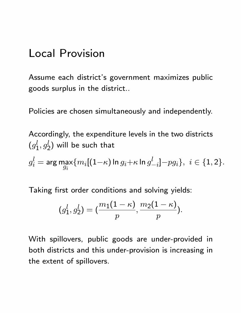
Local Provision

Assume each district’s government maximizes public

goods surplus in the district..

Policies are chosen simultaneously and independently.

Accordingly, the expenditure levels in the two districts

(1 2) will be such that

= argmax{[(1−) ln + ln −]−} ∈ {1 2}

Taking first order conditions and solving yields:

(1 2) = (

1(1− )

2(1− )

)

With spillovers, public goods are under-provided in

both districts and this under-provision is increasing in

the extent of spillovers.

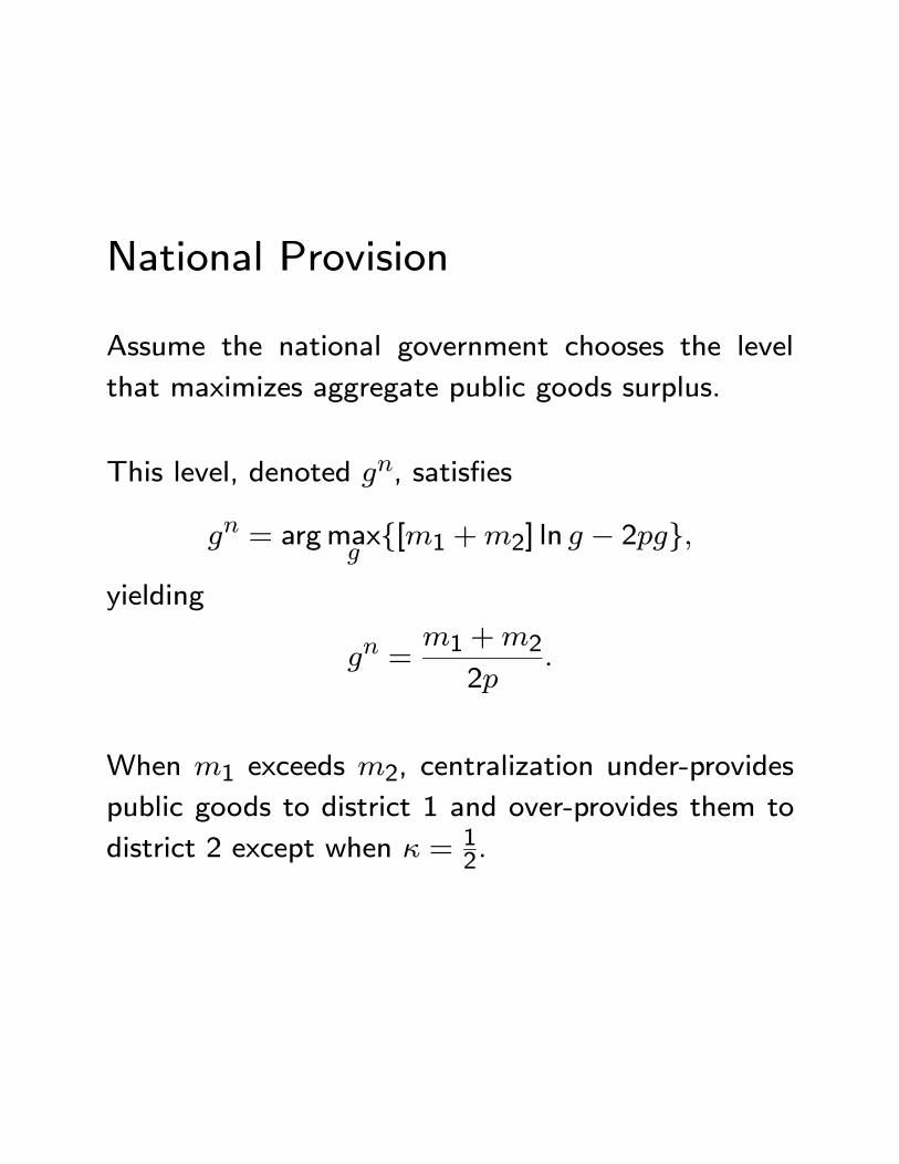
National Provision

Assume the national government chooses the level

that maximizes aggregate public goods surplus.

This level, denoted , satisfies

= argmax{[1 +2] ln − 2}

yielding

=1 +2

2

When 1 exceeds 2, centralization under-provides

public goods to district 1 and over-provides them to

district 2 except when = 12.

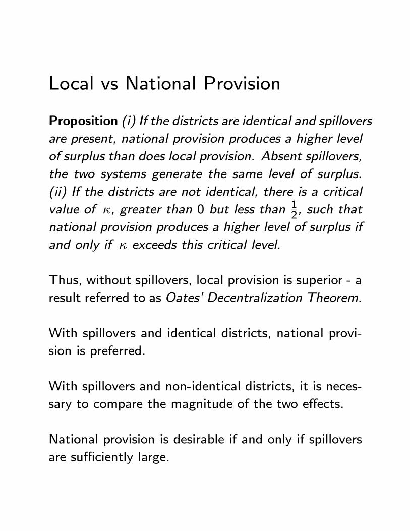
Local vs National Provision

Proposition (i) If the districts are identical and spillovers

are present, national provision produces a higher level

of surplus than does local provision. Absent spillovers,

the two systems generate the same level of surplus.

(ii) If the districts are not identical, there is a critical

value of , greater than 0 but less than 12, such that

national provision produces a higher level of surplus if

and only if exceeds this critical level.

Thus, without spillovers, local provision is superior - a

result referred to as Oates’ Decentralization Theorem.

With spillovers and identical districts, national provi-

sion is preferred.

With spillovers and non-identical districts, it is neces-

sary to compare the magnitude of the two effects.

National provision is desirable if and only if spillovers

are sufficiently large.

IV.8.ii Spillovers vs Preference Het-erogeneity Revisited

The trade-off identified by Oates relies critically on

the assumption that policies under national provision

are uniform across districts.

If the government were permitted to choose different

levels of public goods for the two districts, national

provision is always better.

The justification for the assumption of uniformity un-

der national provision is not completely clear.

One possibility is informational, the national govern-

ment does not know what local people want and there-

fore chooses a “one size fits all” outcome.

Another possibility is that a uniform policy is chosen

on fairness grounds.

Empirically, the uniformity assumption seems reason-

able for things like environmental standards, but not

for spending on roads, parks, etc.

Besley and Coate (2003) compare local and national

provision without the uniformity assumption.

They argue that the sharing of the costs of local public

spending under national provision will create a conflict

of interest between citizens in different localities.

Assuming national spending decisions are made by a

legislature of locally elected representatives, this con-

flict of interest will play out in the legislature.

Thus the performance of national provision will de-

pend upon how the legislature chooses policy.

To make predictions concerning legislative policy-making,

they draw on the citizen-candidate model of elections

and the legislative bargaining approach to legislative

decision-making.

Local Provision

Under local provision, each district elects a single rep-

resentative from among its members to choose policy.

Representatives are characterized by their public good

preferences and a representative of the majority pre-

ferred type is elected.

The policy determination process has two stages.

First, elections determine which citizens are selected

to represent the two districts.

Second, policies are chosen simultaneously by the elected

representative in each district.

To faciltate comparison with Oates, assume that the

median preference equals the mean preference in each

district.

Then, in equilibrium, each district elects a represen-

tative with public good preferences and the policy

outcome is

(1 2) = (1(1− )

2(1− )

)

This is the same as under the Oates approach.

National Provision

Under national provision, each district elects a repre-

sentative to the legislature which then chooses policy.

The legislative bargaining approach predicts that poli-

cies will be determined by a minimum winning coali-

tion and that the identitity of this minimum winning

coalition will be uncertain.

To capture this, assume that if the representatives

are of types 1 and 2, the policy outcome will be

(11(1) 12(1)) with probability 12 and (

21(2)

22(2))

with probability 12 where (1() 2()) is the op-

timal choice of district ’s representative; that is,

(1() 2()) = arg max

(−){[(1− ) ln + ln −]

−2( + −)}

Note that

(() −()) = (

2(1− )

2

) ∈ {1 2}

Given these policy rules, each citizen prefers a repre-

sentative of his own type.

Thus, a pair of representative types is majority pre-

ferred if and only if it is a median pair; i.e., (∗1 ∗2) =(12).

The policy outcome with national provision will be

random, generating (1 2) = (21(1−)

21) with

probability 12 and (1 2) = (22

22(1−)

) with

probability 12.

It follows that there are two drawbacks of national

provision: uncertainty and misallocation across dis-

tricts.

Notice, however, that these problems are attenuated

the greater are spillovers and the lower is heterogene-

ity.

This is because the basic conflict of interest between

citizens in the two localities is lower when spillovers

are high and preferences are similar.

Local vs National Provision

Proposition (i) If the districts are identical, there is

a critical value of , strictly greater than 0 but less

than 12, such that national provision produces a higher

level of surplus if and only if exceeds this critical

level. (ii) If the districts are not identical, there is

a critical value of , strictly greater than 0 but less

than 12, such that national provision produces a higher

level of surplus if and only if exceeds this critical

level. This critical level is higher than that in Oates’

approach.

The bottom line is that the relative performance of lo-

cal and national provision still depends upon spillovers

and differences in tastes for public spending, but for

different reasons than suggested by Oates.

IV.8.iii Voting with your Feet

In a setting of mobile households, local provision of

public goods and services has a number of important

advantages.

First, citizens can seek out jurisdictions with public

outputs that are well suited to their tastes - so called

“Tiebout sorting” (Tiebout (1956)).

Second, in contrast to the monopolist position of na-

tional government, local governments must compete

for residents and this competition mitigates govern-

ment exploitation of their citizens.

Taking a Leviathan view of government, competition

can substitute for explicit fiscal restraints on govern-

ment (Brennan and Buchanan).

Epple and Zelenitz (1981) provide a well-known analy-

sis of this argument.

Consider a geographic area of land size .

The area can be divided into identical jurisdictions

of size , where ≥ 1.

The housing supply function on each unit of land in

the area is ( ) where is the price of housing.

These supply functions are assumed exogenous and

the suppliers are outside the model.

Jurisdiction provides units of a public service to

each resident.

The cost of a unit of service is and service provision

is financed by a property tax .

The total number of households is and the number

residing in jurisdiction is .

Each household has an identical utility function ( )

defined over private consumption , housing , and

public services , and an identical income .

Let

( (1 + ) ) = argmax( − (1 + ) )

denote the individual household’s demand for housing

and

( (1 + ) ) = ( − (1 + )(·) (·) )the associated indirect utility function.

The timing of the model is that: (i) each jurisdiction

chooses a tax-service level (), and (ii) housing

markets open and each household chooses a jurisdic-

tion and housing level.

Housing prices must be such that for each jurisdiction

supply equals demand; i.e.,

((1 + ) ) = ()

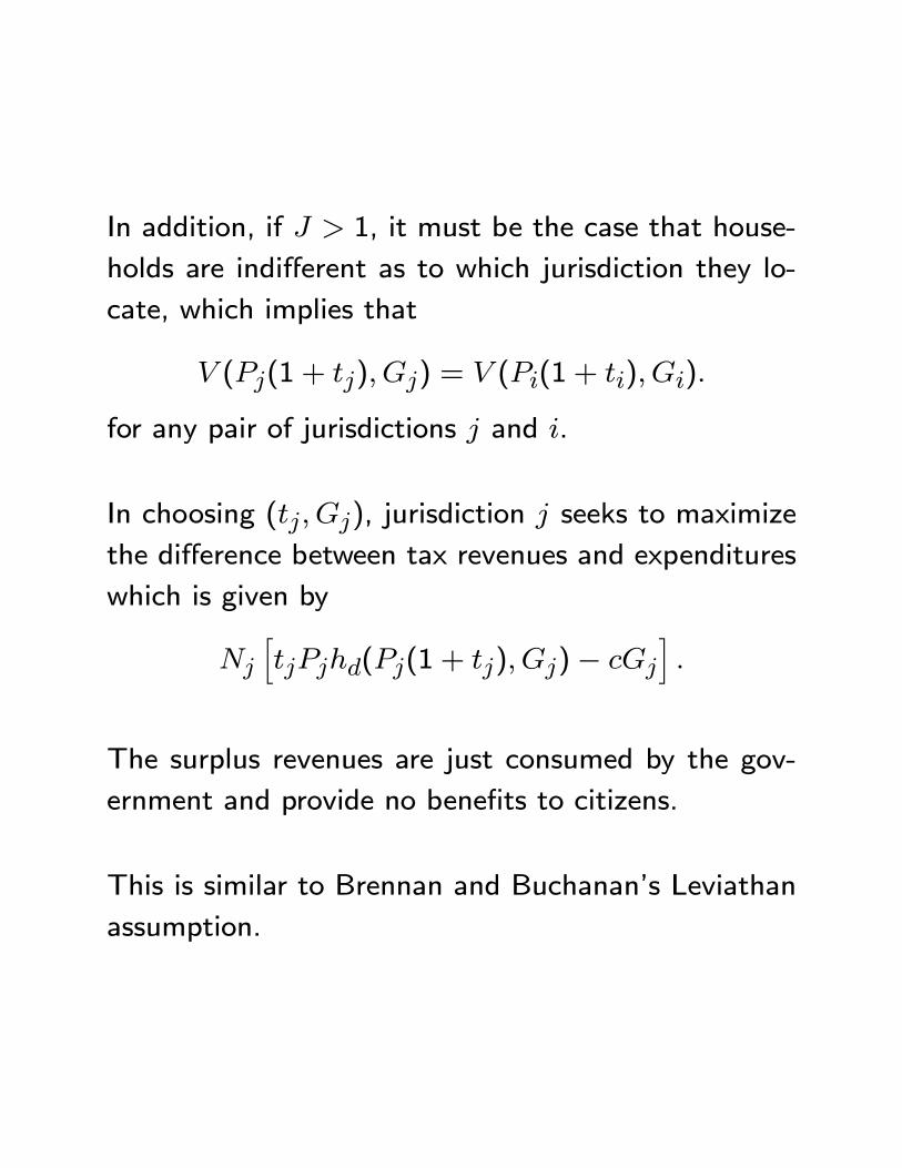
In addition, if 1, it must be the case that house-

holds are indifferent as to which jurisdiction they lo-

cate, which implies that

((1 + ) ) = ((1 + ) )

for any pair of jurisdictions and .

In choosing ( ), jurisdiction seeks to maximize

the difference between tax revenues and expenditures

which is given by

h((1 + ) )−

i

The surplus revenues are just consumed by the gov-

ernment and provide no benefits to citizens.

This is similar to Brennan and Buchanan’s Leviathan

assumption.

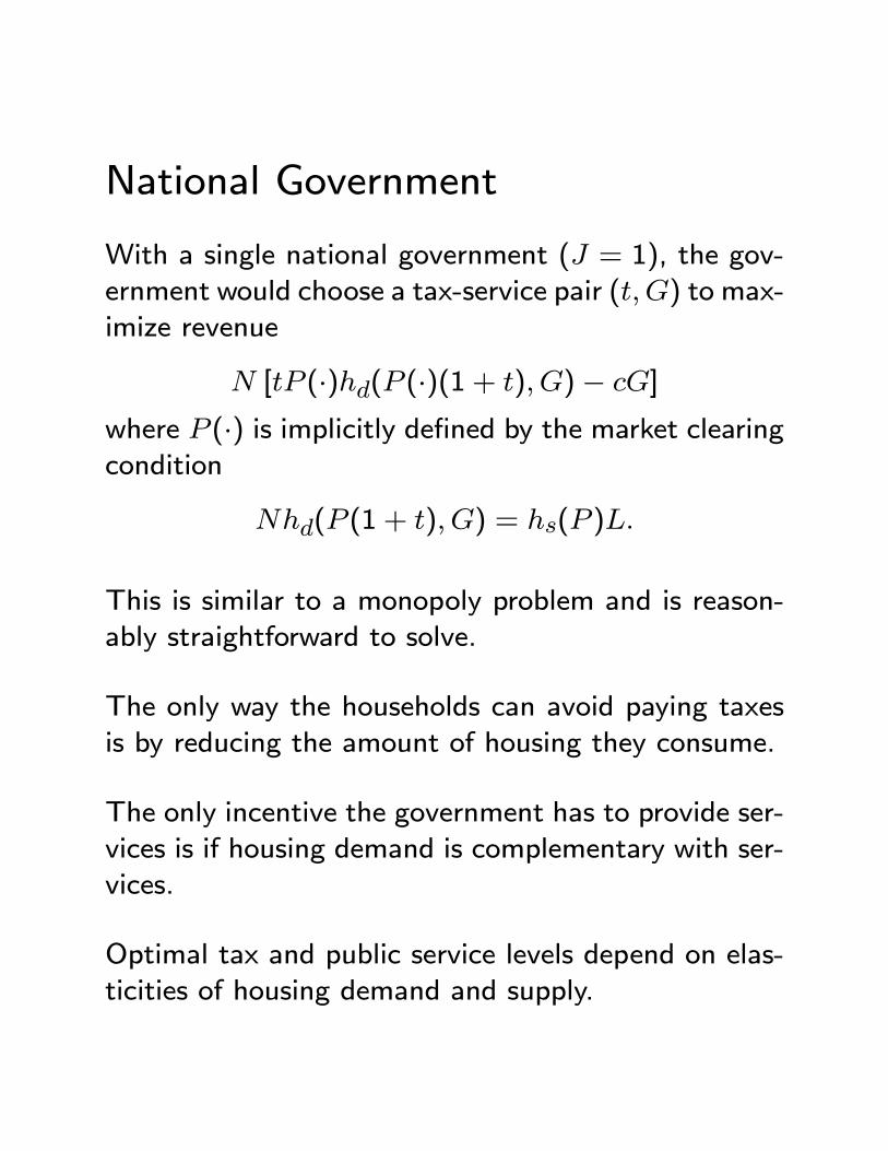
National Government

With a single national government ( = 1), the gov-

ernment would choose a tax-service pair () to max-

imize revenue

[ (·)( (·)(1 + ) )− ]

where (·) is implicitly defined by the market clearingcondition

( (1 + ) ) = ( )

This is similar to a monopoly problem and is reason-

ably straightforward to solve.

The only way the households can avoid paying taxes

is by reducing the amount of housing they consume.

The only incentive the government has to provide ser-

vices is if housing demand is complementary with ser-

vices.

Optimal tax and public service levels depend on elas-

ticities of housing demand and supply.

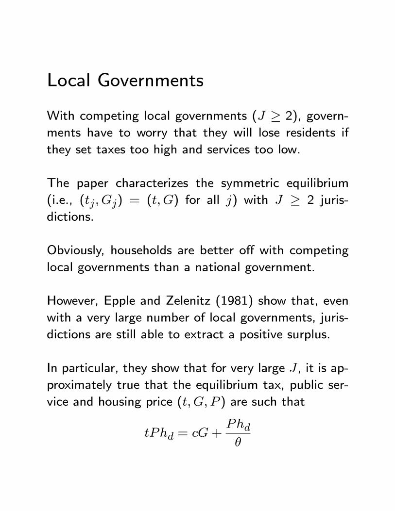
Local Governments

With competing local governments ( ≥ 2), govern-

ments have to worry that they will lose residents if

they set taxes too high and services too low.

The paper characterizes the symmetric equilibrium

(i.e., () = ( ) for all ) with ≥ 2 juris-

dictions.

Obviously, households are better off with competing

local governments than a national government.

However, Epple and Zelenitz (1981) show that, even

with a very large number of local governments, juris-

dictions are still able to extract a positive surplus.

In particular, they show that for very large , it is ap-

proximately true that the equilibrium tax, public ser-

vice and housing price ( ) are such that

= +

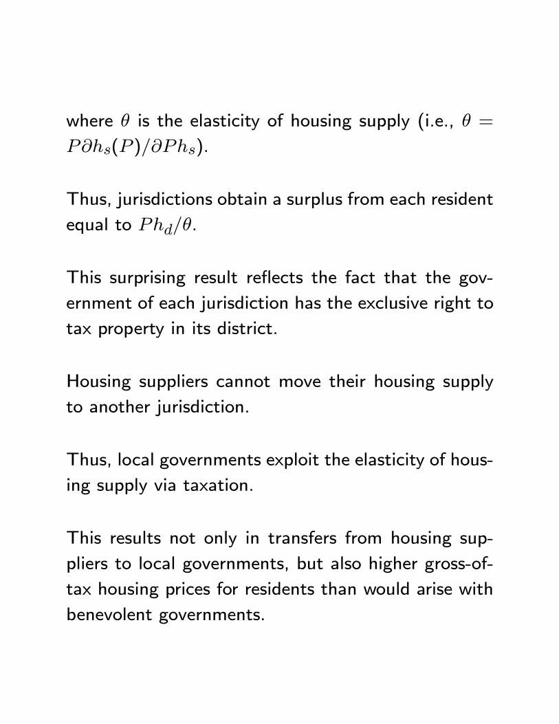
where is the elasticity of housing supply (i.e., =

( )).

Thus, jurisdictions obtain a surplus from each resident

equal to .

This surprising result reflects the fact that the gov-

ernment of each jurisdiction has the exclusive right to

tax property in its district.

Housing suppliers cannot move their housing supply

to another jurisdiction.

Thus, local governments exploit the elasticity of hous-

ing supply via taxation.

This results not only in transfers from housing sup-

pliers to local governments, but also higher gross-of-

tax housing prices for residents than would arise with

benevolent governments.

IV.8.iv Race to the Bottom

An important argument in favor of national rather

than local provision is that local control of policies

can lead to a race to the bottom.

The intuitive idea is that local governments will com-

pete to attract business capital because that will boost

wages and employment opportunities for their citizens.

This competition will result in taxes on business that

are too low.

Similarly, local competition to get business will lead to

environmental standards, workplace regulations, etc

that are too permissive.

By contrast, if business taxes and regulations are set

nationally, there is less concern about capital mobility.

There is a large literature exploring this idea formally.

The simplest models assume that there is a single

mobile factor of production (capital) that is the sole

source of revenue for governments that provide a sin-

gle public service.

Citizens are immobile and government policies are

chosen by the median resident in each locality.

In these models, local service provision results in under-

provision of public services as local governments com-

pete for mobile capital by lowering taxes.

National service provision therefore generates higher

welfare.

If you are interested in this line of argument, you can

start with the chapter in W & W by Wildasin and the

paper “Economic Competition among Jurisdictions:

Efficiency Enhancing or Distortion Inducing” by Oates

and Schwab in the Journal of Public Economics 1988.