NA1ISCELLANEOU& PAPER H4.&5

ICDUNDAR-Y EFFECTS OF UNIFORM SIZEROUGHNESS ELEMENTS IN

TWO-DIMENSIONAL FLOW INOPEN CHANNELS

by

B. J. Brown

Y. 14. Chu

BK

Sponsored by

Assistant Secretary of the Army (R&D)

Department of the Army

Conducted by

U. S. Army Engineer Waterways Experiment Station

CORPS OF ENGINEERSVicksburg, Mississippi

THIS DOCUMENT 4AS BEEN APPROVED FOR PUBUC RELEASEAND SALE; ITS DISTRIBUTION IS UNUMITED

Roprduced by

MATIONAL TECHNICALINFY•MATION SERVICE

sp.. " fiJ:,• VýV 22151

Unclassifiedsocugitir classifteation

DOCUMENT CONTROL DATA. 3 & DS2"wdey 91-Anlklj .1 sfP 5.' .1 ah.imct sew I*ndeant smetetSe mus~t 6.0 entered JIM me *Wotan report Is eCANS811104

I-ORIGINATING ACTiVITY (Corporte 00") J a. REPORT SECURITY CLASSIFICATION

U. S. Army Engineer Waterways Thcperiment Station Unclassified* Vicksburg, Mississippi ASbG, u

11. REPORT TITLE

BOUNDARY EFFECTS OF UNIFORM SIZE ROID1HiESS ELRMENTS IN TWO-D2MENSIONAL MMJ IN OPENCHANNELS

d. OESCRIPIVE NtOTES (2V'p GIM~ot And 5.dI*.*,. dft*)

* Final reportG . AUTMORIS) (First memo. F1d.- iAtti. A~est nst)

Bobby J. BrownYen H. Chu

.. REPORT DATE T&. TOTAL NO. OF PAGES 76. NO. or RaeS

December 1968 67 17is. CONTRACT ON GRANT NO. an. ORIG8INATOWS REPORT NU&MURISI

h.PROJECT NO. Miscellaneous Paper H-68-5

S. .g. OTHER REPORT NOISI (AW GStAW ont.I filla SWi? SO*#~

Is. DSTMOUTOON STATEMENT

This document has been approved for public release and sale; its distributionis unlinited.

II. SUPPLENMETARY MOTES Ia.* SPONSORING WLITARY ACTIVITY

Assistant Secretary of the Arnry (R&D)

.5. USTA cnduced o ivestgat th 1Department of the Army

ests wrcodcetoivsiaehecharacteristics of the vertical velocity dis- 1tribution in flow inwide channels with large relative roughness. The study wasbasically a two-dimensional investigation of the boundary roughness effects inturbulent flow. The investigation was conducted in a !48-ft-long, 2-1/2-ft-wideflume with 1/8-, 1/2-, 3/4-, and 1-in, crushed limestone and 3/4-in, concrete cubesas the boundary roughness. Results indicate that the root-mean-square value '-e--of the boundary roughness heights is related to the Nikuradse equivalent sand grainroughness *6L~- and that the root-mean-square value can be treated as a roughnessparameter for boundaries of dense:ly spaced, irregular, randomly placed roughnesselements of uniform size. Appendix A includes the experimental data. Appendix Bdescribes the special instrumentation used for measuring the vertical velocity pro-files within the flow.

D o"W'w1473 ::J:~:G A G fMMUnclassified

•immm•i [ i•.Unclassified

x ~kw woN0 @ £ LUS II

ROLZ W? oE ILK WT

Boundary layer flow IChannel flow

Open-channel flow

Roughness

Two-dimensional flow

uinclassif'ied

- amNNY

!!I•

MISCELLANEOUS PAPER 1-68-5

BOUNDARY EFFECTS OF UNIFORM SIZEROUGHNESS ELEMENTS IN

TWO-DIMENSIONAL FLOW INOPEN CHANNELS

by

B. J. BrownY. 14. Chu

December 1968

ý0* Sponsored by

Assistant Secretary of the Army (R&.D)Department of the Army

Project ILO1300IA91AItem L

Conducted by

_U. S. Army Engineer Waterways Experiment StationCORPS OF ENGINEERS

Vkkbuv, MK"sisppi

ii ~i

T141S DOCUMENT WAS BEEN AIPPROVED FOR PUBUC RELEASEAND SALE; ITS DISTRIBUTION IS UNUMITED

ii i '

i Asd~n Sce!ryo teAry(RD

== =

iII

THE CONTENTS OF THIS REF\)RT ARE NOT TO BE

USED FOR ADVERTISING, PUBLICATION, OR

PROMOTIONAL IURPOSES. CITATION OF TRADE

NAMES DOES NOT CONSTITUTE AN OFFICIAL EN-

DORSENENT OR APPROVAL OF THE USE OF SUCH

CONMERCIAL PRODUCTS.

iiii

.9

IYI

FOREWORD

This study was funded. by Department of the Army Project 1LO13001A91A,

"In-House Laboratory Independent Research Program.," Item L., sponsored by

the Assistant Secretary of the Army (R&D). It was conducted during the

period July 19641 to Jul-y 1968 at the U. S. Arqy Engineer Waterw.ays Experi-

ment Station, Vicksburg., Mississippi, under the direction of Mr. E. P.

Fortson., Jr.., Chief,, Hydraulics Division. The study was assigned to the

Analysis Section of the Hydraulic Analysis Branch. Messrs. F. B. Campbell

and E. B. Pickett were, successively, Chiefs of the Hyrdraulic Analysis

Branch, and Mr. R. G. Cox was Chief of the Analysis Section during the

study.

The initial phase of the study, 28 July 1964 to 3 September 1965, wasaccomplished 'by SP 4f J. S. Watkins under the technical supervision of

Mr. Pickett. During this period the test facility building was constructed.,

the test equipment was designed, fabricated, and instal-led, and an exten-

sive literature search was completed. SP Watkins' duty tour ended in

September 1965.

The project was generally inactive during the period September to

December 1965., at which time Mr. B. J. Brown was assigned as project engi-

neer under the technical supervision of Mr. Cox. During the period 6 De-cem~ber 1965 to 20 April 1966, the test facility and equipment were checked

out and the first experimental data were obtained. A First Interim Report

dated April 1966 was prepared by Mr. Brown and describes the test proce-

dures used and test data and results obtained with two types of flume in-

vert roughness. Mr. Brown left for military duty in mid-April 1966.

Second and Third Interim Reports were prepared by Mr. Y. H. Chu,,

1v

S ••• •w • , • • Ar•' • •'• • •* " '•V

iiydrw~~zlic -eer ngnc ad. Sp q- _T r,%,. Aimiiu the pneriod. SepteM-

ber 1966 to October 1967.

Mr. Brown (CPT, USAR) was assigned to the project in a military

capacity during the period 1 Februazyr to 21 April 1968 and subsequently

reassigned as civilian project engineer on 22 April 1968 upon completing

his tour of active duty.

This, the final report on the study, summarizes all the test data

and results to date. The report was prepared by Messrs. Brown and Chu.

The basic data were obtained and analyzed by SP Canton during the period

September 1966 through January 1968.

Directors of the Waterways Experiment Station during the conduct of

the investigation and the preparation and publication of this report were

COL John R. Oswalt, Jr., CE, and COL Levi A. Brown, CE. Technical Director

was Mr. J. B. Tiffany.

vi

CONTENTS

Pag

CONVERSION FACTORS, BRITISH TO METRIC UNITS OF MEASUREMENT . . . . o xi

PART I: INTRODUKTIONo o o . . . . . .. . ... . . . .. .. .. . 1

PART" II: TEST APPARATUS o o . o . . o o . o . o o o . . . o . . o 4• Description of Test Facility . ........... .. . . 4

Equipment . . . . . o o . o . o o . . . . 5

PART III: TEST CONDITIONS AND PROCEDURES .............. 7

Establishment of Test Flow . ....... .. ..... ... 7Discharge and Bed-Slope Adjustment .............. 7Vertical Velocity Profiles . ................. 8Boundary Roughness . o * . ... . . . . ... .. . . .. .. 8Evaluation of Shear Velocity . ............ ... . 12Determination of Theoretical Flow Boundary . . .0. . * . . 13Nikuradse's Equivalent Roughness Height (ks) o . . o . . . . 14

PART IV: RESULTS AND DISCUSSION .. ... ......... ... 15

Boundary Roughness . . .0. .0 . .0 . . . . ... .... . ... 15Velocity Distribution ......... ...... .... . 17Resistance Coefficients. . . . . . . * . 0 . . . . . . . . . . 18

PART V: CO!"LUSIONS AND COMENTS o .. . ....... . .... . 19

LITERATURE CITED .e. .o * * . . .e. . . . .. . . .. . . .. .. 20

PLATES 1-16

APPENIqDJ A: TEST DATA . . . . . . . . . 0 0 o . * o 0 0 a o . . o . Al

TABLES Al-AlO

APPEINDEJX B: CALIBRATION OF 1/8-IN. PITOT TUBE AND DIFFERENTIAL| •PRESSURE TRANSDUCERS ...... o* **... *............ Bl"PInstruments oI . . . . . . . . . . . . . . . . . . o . o B1

Static Calibration. o o . 999 BI

vii"]

i I r - -- **o* •--.-

Dynamic Calibration . . . . . . . . . . . . . . . . . . .... B2Discussions . . . . ... 0. .. . .. . . B2

Operation Comments . . . . . . ............... B3

PLATES Bl-B5

v

viii

S1~

III

NOTATlION

a,b,c axial radii of the stone

C 'hezy's resistance coefficient

d corrected flow depth, ft

D mean stone diameter, ft50f Darcy-Weisbach friction factor

g gravitational acceleration, ft/sec2

h vertical distance measured from top of roughness, ft

k effective roughness height, ft; k = 2 a

k Nikuradse's equivalent sand grain roughness, ft

n Manning's roughness coefficientj N number of point gage readiis

Q discharge, cfs

R hydraulic radius

i SO slope of flume bottom, ft/ft

S i slope of water surface relative to flume bottcm, ft/ft

S.F. shape factor of roughness elements

U velocity at distance y from boundary, ft/sec

U mean velocity along center line of flume, ft/sec

_U shear velocity, ft/sec

X point gage reading, ft

I mean point gage reading, ft

y vertical distance above nominal flow boundary, ft

y specific weight of fluid, ib/ft 3

X concentration factor

ix

distance beneath top rougnhess surface to fo=a i'...boundary, ft

p unit mass density; 1.94 slugs/ft 3

a root-mean-square value of roughness protrusions, ft

o average shear stress at the boundary, lb/.t

x

III|

CONVERSION FATORS., BRITISH TO METRIC UNITS OF MEASUREMEN

British units of measurement used in this report can be converted to metric

units as follows:

multiply ByTo Obtain

inches 2.54i centimeters

feet 0.3048 meters

pounds per square foo .84 kilograms per square meterpounds per cubic foot 16.0185 kilograms per cubic meter

feet per second 0.30148 meters per second

feet per second per second 0.3048 meters per second per second

slugs per cubic foot 515.7957 kilograms per cubic meter

cubic feet per second 0.0283168 cubic meters per second

Fahrenheit degrees 5/9 Celsius or Kelvin degrees*

*To obtain Celsius (C) temperature readings from Fahrenheit (F) readings.,use -thbe following formula: C =(5/9) (F - 32) .To obtain Kelvin (K)readings, use: K =(5/9) (F -32) + 273.16

xi

SUNMARY

Tests were conducted to investigate the characteristics of the verti-cal velocity distribution in flow in wide channels with large relativeroughness. The fstudy was basically a two-dimensional investigation of theboundary roughness effects in turbulent flow. The investigation was con-ducted in a 48-ft-long, 2-l/2-ft-wid~e flume with 1/8-, 1/2-., 3/4-,, and1-in. crushed limestone and 3/ 4 -in. concrete cubes as the boundary rough-ness. Results indic-ate that the root-mean-square value a of the boundaryroughness heights is related tu the Nikuradse equivalent sand grain rough-ness k sand that the root-mean-equare value can be treated as a roughness

* parameter for boundaries of densely spaced, irregular, randomly placedroughness elements of uniform size. Appendix A includes the experimentaldata. Appendix B describes special instrumentation used for measuringthe vertical ve:L-city profiles within the flow.

xiii

BOUNDARY EFFECTS OF UNIFORM SIZE ROIXGHNESS EISHEWI

IN TLWO-DIM4ENSIONAL FIW IN OPEN CHANNELS

PART I: INTRODi.ETIO

1. It is co flJy assumied that the law of universal velocity dis-

tribution applies in open-channel hydraulics; however, difficulties still

I= I

t exist that limit its practical application. The purpose of the study de-

scribed. herein was to investigate the characteristics of the vertical ye-

locity distribution in flow in wide channels that have a large relative

roughness. An attempt was made to accurately measure the variables in-

volved in the basic law and to rationalize their effects. A statistical

approach for defining the boundary roughness was used in the study, and the

results have been correlatedwidth Nikv-cadse' s equivalent sand grain rough-

ness (k s) Chezy's resistance coefficient (C), and the Darcy-Weisbach fric-

tion, factor (f) for the roughnesses considered.

2. Keulegan showed that the Prandtl-von Karman universal velocity

distribution law for pipe flow could be applied to open-channel flow.2Based on a theoretical analysis and an analysis of Bazin's data for rough

channels, Keulegan founde that the equation

U 8.5+ 575 log1 ()

described the vertical velocity profile of turbulent flow in a rough chan-

nel, where U is the local velocity at a distance y above the flow

boundary.. Ut is the shear velocity, and k is Nikuradie'es equivalent

sand grain size. Integrating equation 1 over the total depth gives the

mean velocity of flow in the form

U = 6.25 +5.75 log Y (2U* k

iiiwhere U is the mean velocity of flow.

!.!!! I1

3. Considerable research has'been conducted on flow in rough chan-nels since Keulegan published his classical paper in 1938. However, most

of it involved the use of artificial blocks, bars, or spherical balls as

the channel bottom roughness. Powell experimented with small rectangular

sills, Robinson and Albertson used baffle plates, and Moore, Rand, and

Hama5 used transverse bars of vaeious sizes. All of these studies were

similar, and Chezy's C was used to describe the flow resistance. Little

research has been done on channels with boundary surfaces composed of

large-scale natural roughness. The present study was undertaken to provide

"information on the vertical velocity distribution in turbulent flow in

rough, open channels and to seek a better measurement of Aatural channel

roughness than the commonly accepted nominal stone size.

4. The traditional Manning's n lacks a scientific method for pre-

diction and was not employed in the present study. A universal roughness

parameter such as Nikuradse's equivalent sand grain diameter ks may not

necessarily be represented by a single dimension of roughness height.

Schlichting6 reported that different distribution patterns of artificial

roughness in his laboratory conduit resulted in different values of ks

which were not comparable with the actual dimensions of roughness elements.

Recent results from Koloseus and Davidian indicate that a concentration

factor (X) of boundary roughness as well as the geometric properties of

individual elements was required for predicting the k of a given bound-

ary. At the present time, the ) valve can be controlled and apprcximated

only for roughness of uniform shape, size, orientation, and arrangement. A

practical parameter of roughness is still required when k cannot be

readily determined. A procedure for describing the roughness characteris-

tics of a boundary surface in terms of the root-mean-square value c of

the surface protrusions is given herein.

5. This report summarizes the results of tests conducted with 1/8-,

1/2-, 3/4-, and i-in.* crushed limestone rock-'and 3/4-in. concrete cubes as

the channel bed roughness. Size identification of the crushed stone is the.. minimum sieve size upon which the particles were retained during screening

A table of factors for converting British units of measurement to metricunits is presented on page xi.

2

1|1

operations. The square mesh openings of the sieve that passed the test

ro~ck were 1/4 in. larger than those that retained it. The 1/8-in. size

passed the No. 4 sieve and vas retained on the No. 8 sieve. Three interimi• o ! reort8,9,!Oreports published on the study include all the data except for the

1/8-in. stone and 3/4-in. concrete cubes. All the test data are presented

herein in Appendix A.*

II

I

Si 3•

PART II: TEST APPARATUS

Description of Test Facility

6. The general layout of laboratory equipment is shown in fig. 1.

The recirculating flow system consisted of the sump, the pump, the supply,•~•pipes, the hedbay., and the flume. The test flume., 48 ft long, 2-1/2 ftwide, and 1-1/2 ft deep, was of steel construction and equipped with a

sensitive, electrically operated tilting mechanism. The slope range was

from a maximum slope of 0.015 to a maximum adverse slope of -0.005. The

reference datum for vertical measurements consisted of two rails mounted on

the flume sidewalls parallel to the flume bottom. The test section was

38.5 ft downstream from the flume entrance, at a location where the turbu-

lent boundary layer was considered to be fullv developed. Approximately

uniform depth in the flume was obtained by adjusting a chain-driven, under-

shot tailgate. The supply pipe consisted of a 10-in, main with a 10- by

Fig. 1. View of test flume, looking downstream

4

5-in. venturi tube and a 6-in. bypass with a 6- by 3-in. venturi tube.

The venturi tube pressure differentials were read by means of a mercury

SU-tube manometer. Discharge was controlled by valves located between the

venturi meters and the flume headbay.

Equipment

7. Various commercial and homemade pitot tube and manometer systems

were used in an effort to obtain optimum velocity measurements. The in-

ability to repeat meas-

urements greatl~y reducedthe reliability of such

systems, especially in

measuring the low flow

velocities. The most

* ireliable pitot tube-

manometer system was a

5/16-in.-OD, commercial,

Prandtl-type pitot tube

and a shopmade, 1:10-sloping manometer

(fig. 2). Velocity data

with the 1/2- and 1-in.

stone and the 3/4-in.

cubes as the boundary

roughness were obtained

using this equipment.

Initially the system re-

quired a long settling

period between readings

and frequently produced

unsatisfactory variations

in the velocity when Fig. 2. 5/16-in. pitot tube and

S.checks were made at sloping manometer

g5

arbitrary locationsi it the profile. Both instrument response and measure- *n

ment repeatability were improved by injecting several drops of an aerosol

solution into the water column of' the inclined manometer. The instrumentwas calibrated in a 14-ft-diam rotating calibration tank; the basic cali-

bration curve is shown in plate 1.

8. Improved accuracy in the velocity measurement was made with the

use of a variable-reluctance differential pressure transducer in conjuic-

tion with a 1/ 8 -in. pitot tube. A complete description of the instrument,

calibration, and operating procedure is given in Appendix B.

6

-~i -

PART III: TEST CONDITIONS AM POCKDNOR

Establishment of Test Flow

9. The basic ideal requirements for establishing the test flow were

to: (a) obtain uniform flow over sufficient flume length, and (b) maintain

two-dimensional flow in the flume within practical limits. Exactly uniform

flow could not be expected, principally because of insufficient flume

length for the resistance and gravity forces to balance each other. How-

ever, relatively uniform flow was obtained by carefully setting the flume

tailgate. Adjustments were also made in the analytical procedure when the

flow appreciably deviated from the general assumption of uniformity. This

adjustment is described in paragraph 21. Flows at a small Froude number

were desirable to minimize instabilities resulting from surface waves.

10. Two-dimensional flow can only be assumed with flows at large

width-to-depth ratios. The present tests were limited to ratios between

5 and 10, which corresponded to flow depths of 0.5 to 0.2 ft, respectively.

Within this range, the following crit' *.a were obtained: (a) the relative

roughness became large, (b) the Froude number was less than unity, and

(c) sidewalls and secondary currents had negligible effect upon the center-

line velocity profile.

Discharge and Bed-Slope Adjustment

.1. Selections of discharges and flume slopes were arbitrary, pro-

viding they did not produce depths that would not conform to the criteria

in paragraph 10. The slopes used were 0.0023, 0.0030, 0.0040, and 0.0060o.

The minimum slope was governed by the sensitivity of velocity measuring

equipment and the possibility of the proportionally greater error involved

in determining the energy gradient. The maxil-um slope depended upon the

Froude number of the flow, which was related to the surface stability at

the desired width-depth ratio. The discharge varied from 0.75 to 2.50 cfs

in order to meet the required depth at the selected bed slope.

7

IJ

"Vetic. ,.ca. Velocity..Pr *,.a-

12. The primary interest of the study was the vertical velocity dis-

tribution for fully developed, turbulent, two-dimensional, uniform flow.

Therefore, at the beginning of testing it was necessary to select the

proper location in the flume where these conditions were most nearly ful-

filled. C.lection of the location, 38.5 ft from the channel entrance and

hereafter called the test section, was based on the results of detailed

velocity traverses taken at several locations along the length of the

flu1me. The velocity traverses indicated that symmetrical flow conditions

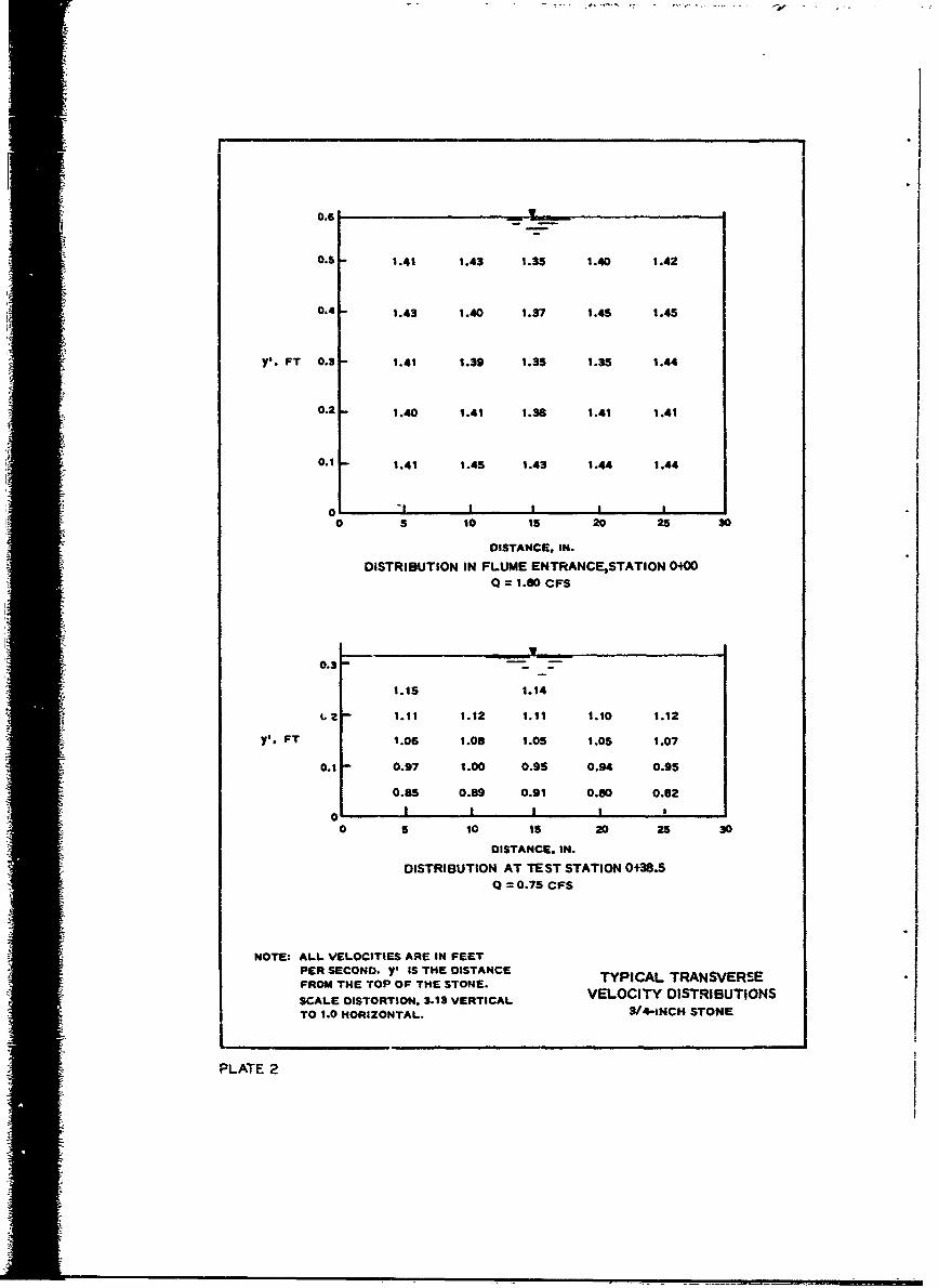
existed in the flume. Plate 2 shows that potential flow generally existed

at the flume entrance and that the flow at the test section was symmetrical

and the turbulent boundary layer fully developed. Detailed vertical veloc-

ity profiles were measured at the center line. Measurements in the verti-

cal were generally made at intervals of 0.02 ft near the boundary and at

larger intervals near the free surface. The higher velocities measured at

a slope of 0.0060 were obtained by extrapolating the pitot tube calibration

curve.

Boundary Roughness

13. Tests were conducted with four different uniform sizes (1/8,

1/2, 3/4, and 1 in.) of crushed limestone rock and one size (3/4 in.) of

concrete cubes (see fig. 3); size identification is described in para-

graph 5. The crushed stone (except the 1/8-in, stone, which will be de-

scribed later) was initially placed and spread in the flume with shovels.

No attempt was made to spread the stone at a prescribed thickness, but

generally the average thickness was about twice the nominal stone diameter.

in accordance with the requirement for uniform flow, the stone layer was

carefully leveled with reference to still-water surface. The flume was

positioned horizontally and flooded to a depth at which the water surface

was level with the highest stone protrusions. A mason's trowel was used

to level and lightly compact the layer with reference to the water surface.

S14. The 1/8-in, stone was cemented to the flume bottom with a

S8

SI8

* A

It I

a. 1-in. stone b. 3/4-in. stone

UPii

c. 1/2-in, stone d. 1/8-in. stone

e. 3/4-in, cubes

Fig. 3. Flume bed. roughness

plastic adherent to prevent displacement at the hIgher .... s. The

flume bottom was coated with a thin layer of adherent, and the stone was

evenly spread to a layer thickness of approximately twice the nominal

stone diameter. The loose particles were "washed out" after the 6dherent

hardened.

15. The 3/4-in. concrete cubes were placed upon a layer of 3/4-in.

stone to obtain the desired irregular surface (fig. 3e), and the surface

was leveled as Oescribed in paragraph 13.

_16. Determination of the stone characteristics given in the tabula-

tion on page 15 for each stone size was made from measurements of 100 ran-

domly selected stones. Small shovelfuls of stone were obtained from sev-

eral locations within the flume or from the stockpile and placed into one

sample. The large sample was qrartered into sixteen test specimens, ten

of which were randomly selected and the remaining six discarded. A small

box w - constructed in which the bottom was divided into a 10 by 10 grid

(100 snll. squares). Each square was assigned a nimber, and each number

was recorded on a separate piece of paper which was placed in a container.

One of the ten test specimens was placed in the box and spread until each

square was occupied by a stone particle. The excess particles were re-

moved. Ten numbers were drawn from the container and the particles occupy-

ing the corresponding numbered squares were selected. Consequently, ten

particles selected from each of the ten specimens produced 100 stones for

measurement. Because of the small variation in size and shape of the

1/8-in. stone, the 100 particles were randomly selected by hand from the

stockpile.

17. Twc methods for determining the effective roughness height of

the boundary inughness were investigated. The first method involved meas-

uring the three axial diameters of stone sxrples from which the average

diameter D50 and shape factor S.F. were computed. The bar graphs in

plates 3-6 indicate the mean diameters and shape factors for each size of

test stone. The 100 randomly selected stones (paragraph 16) were measured

with a hand caliper, and the mean diameter D50 for each stone size was

computed according to the equation:

10

" D = 2(abc)l/3 (reference U1) (3)50

l where a , b , and c are the three axial radii of the stone. The shape

factor S.F. is defined as

=cS.F. = e (reference 12) (4)

where a> b>c

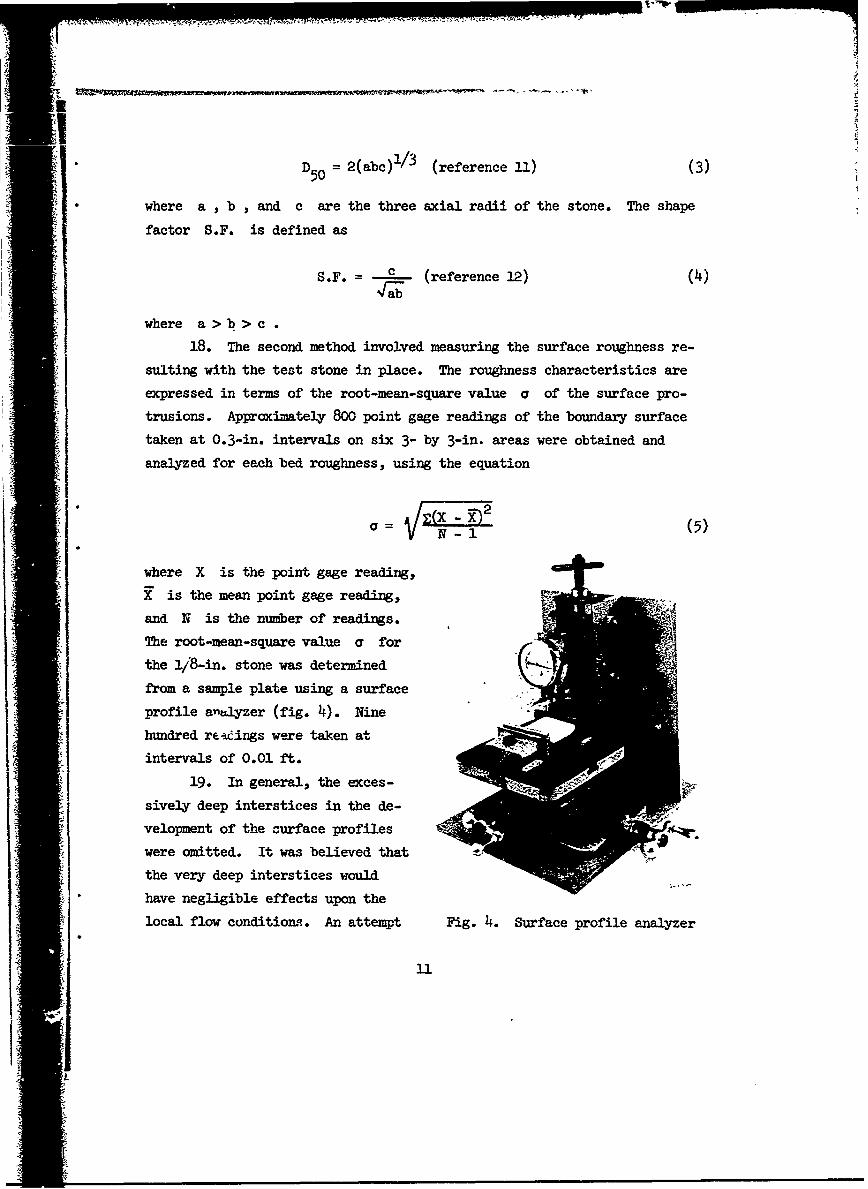
18. The second method involved measuring the surface roughness re-

sulting with the test stone in place. The roughness characteristics are

expressed in terms of the root-mean-square value a of the surface pro-

trusions. Approximately 800 point gage readings of the boundary surface

taken at 0.3-in. intervals on six 3- by 3-in. areas were obtained and

analyzed for each bed roughness, using the equation

* -X2a- ~~E-~-(5)

where X is the point gage reading,

X is the mean point gage reading,

and N is the number of readings.

The root-mean-square value a for

the l/ 8 -in. stone was determined

from a sample plate using a surface

profile anhlyzer (fig. 4). Nine

hundred reaings were taken ate

intervals of 0.01 ft.

19. In general, the exces-

sively deep interstices in the de-

velopment of the surface profiles &

were omitted. It was believed that

the very deep interstices would

have negligible effects upon the

local flow conditions. An attempt Fig. 4. Surface profile analyzer

311

was made to evaluate the effects or tnese cmissions on tne a value. T•is

was accomplished by first arranging the measured readings in numerical se-

quence. The a values were successively computed using a predetermined

percentage increase in the number of readings omitted. Each computed value

was divided by the a value resulting (using all the data) and plotted as

a function of the percentage of total data points used. Typical measured

* -profiles are shown in plate 7, and the results of this statistical study

are shown in plate 8. Reasonable correlation of all surfaces was obtained

except that resulting with the 3/4-in. stone. Plate 8 indicates the gen-

eral relation between the successive elimination of the deeper interstices

and the resulting a

- •Evaluation of Shear Velocity

20. Shear velocity is defined by

U* =, u= (6)

where p is the unit mass density of the fluid and r is the boundary

shear stress. For steady, two-dimensional, uniform flow, -o can be deter-

mined by the equation:

Tii ydS 0 (7)

and therefore

U*= 4b dgS (8)

where d is the corrected flow depth, y is the specific weight of the

fluid, g is the gravitational acceleration, and S0 is the slope of flume

"bed or piezometric gradient for uniform flow.

21. The water-surface profile was measured with a standard point

gage which could be read to 0.001 ft by means of a vernier scale. Meas-

urements were taken at 1- to 2-ft increments from a distance approximately

Ill I1I

. 20 ft upstream to about 4 ft downstream of the test section. In certain

cases, when the mean slope of the water surface differed from the flume

slope, the following modified form of equation 8 was used:

U*~. VIg (9 d- ýs (9)0 w

where S is the slope of the water surface relative to the flume bottom

and it may have a positive or negative value. Equation 9 was derived as-

suming a hydrostatic pressure distribution because Sw is small compared

to S0

Determination of Theoretical Flow Bonry

22. The determination of the effective datum for vertical ordinates

is of considerable significance because of the large relative roughness

: • "used in the study. Neither the bottom of the flume nor the top stone sur-

face can be considered as the effective datum of flow. Initially, this

datum was assumed to be located at a distance D 5/2 beneath the top sur-

face of roughness. A second procedure assumed the effective boundary to

be located at a distance a beneath the top surface of roughness. A third

procedure was recomended by Mr. F. F. Escoffier, WES hydraulic consultant.

23. Mr. Escoffier's procedure assumes that

•~ -' = h +C

where y is the vertical ordinate of the point velocity in the flow, h

is the distance between this position and the top of the stone surface,

and g is the distance beneath the stone surface to the theoretical flow

boundary. Plate 9 sbows the schematic relation of a , g , k , h y p

and d and the ideal velocity profile. The following relation is obtained

using the ,uiversal velocity distribution law for rough boundary:

h + E e-p (0-4 U (10)

13

(0V.4 u\.I-Men thp~ yqeasured h is nilotted against the value of exp (2. U~- inCartesian coordinates, either C or ks can be determined graphically

for a specific set of data. A detailed illustrated example of the pro-

cedure i, given in plate 10.

Nikuradse's Equivalent Roughness Height (k )

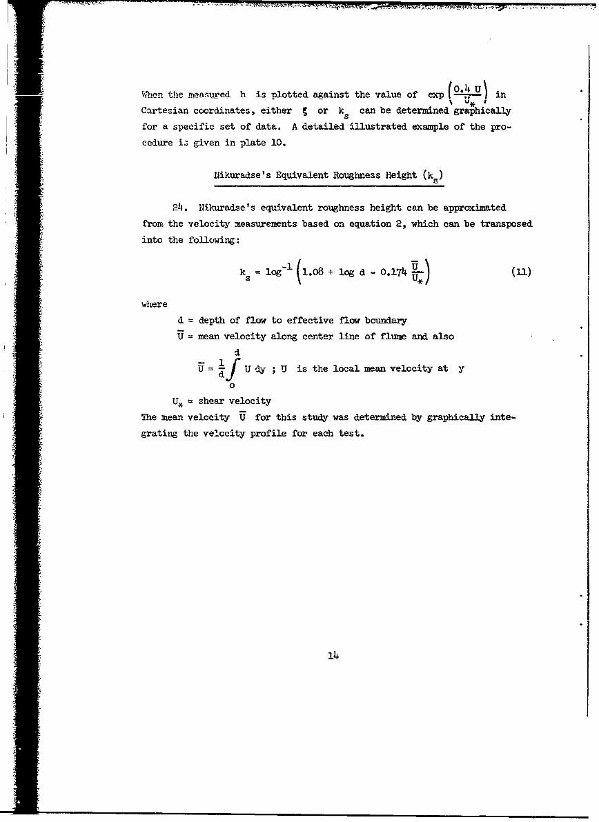
2h. Nikuradse's equivalent roughness height can be appraximated

from the velocity measurements based on equation 2, which can be transposed

into the following:

k s= log'!1.08 + log d - 0.174 ). Wl)

where

d = depth of flow to effective flow boundary

U = mean velocity along center line of flume and also

d

U = U dy ;U is the local mean velocity at y

0

U. = shear velocity

The mean velocity U for this study was determined by graphically inte-

grating the velocity profile for each test.

14

'I " I

PART IV: RESULTS AND DISCUSSION

Boundary Roughness

Stone characteristics

25. The actual surface configurations of the five boundaries are

shown in fig. 3. The bar graphs in plates 3-6 indicate the mean diameter

and shape factor for each size of stone based on random sampling. The

mean diameter D5 0 , shape factor S.F. , and corresponding a value are

summarized in the following tabulation:

Stone Size, in.

I'1/8 1/2 3/4 1 3/4-in. Cube

S.F. o.62o o.46o o.485 0.510 1.000

. ft 0.01036 0.055 0.080 0.106 0.083

a , ft 0.00360 0.0148 0.0181 0.0272 0.0236

k , ft 0.0072 0.0296 0.0362 0.0544 0.0472

k/D50 0.695 0.538 0.452 0.513 0.569

The mean shape factor for three of the four stone sizes tested is approxi-

mately 0.5. The higher value for the 1/8-in. stone is attributed to the

small variation between the three axial diameters. In fact, differentia-

tion between the three diameters was often difficult. The ratio of the

effective roughness height k (k = 2 a) to D5 0 is relatively constant

"except for the 1/8-in, stone. However, the same relation may not exist

among other types and gradations of roughness elements.

i- ii , ks , and C

26. Determination of k and g according to equation 10 is il-

lustrated in plate 10. The accuracy of the results using this procedure

depends upon the measured and computed values of U and U* , respectively.

_ The ratio C/a as shown in the following tabulation varies appreciably,

but excluding the 1/8-in, stone, the average value is about 1.21, which is

close to the assumption for C/a used in the initial procedure (para-

graph 22). The average C/a value for the 1/8-in, stone is about 3.5.

* Indications are that the concentration or distribution of roughness

15

SRock Dis- IRock Ds -- U k t k tt k tt:• • Size enuxge U dss _s

in. S e-s fr. ft ft ft k a

1 0.0023 1.50 1.495 0.174 0.407 0.156 0.155 2.88 0.270.0023 1.75 1.631 0.181 0.444 o.147 0.152 2.80 0.420.0023 2.00 1.687 0.192 0.497 0.177 0.192 3.54 0.94o.oo4o 2.00 2.017 0.232 o.417 0.154 0.175 3.22 1.080.0040 2.50 2.217 0.252 0.493 0.174 0.206 3.72 1.050.0060 2.50 2.658 0.294 0.4V6 0.143 0.202 3.70 1.6 5

3/4 0.0023 1.00 1.281 o.159 0.341 0.155 0.212 5.86 2.770.0023 1.50 1.587 0.171 0.394 0.122 0.127 3.51 1.830.00o 4 1.75 2.029 0.222 0.370 0.109 0.135 3.73 1.710.0060 2.00 2.313 0.270 0.378 o.138 o.164 4.53 1.59

1/2 0.0023 1.25 1.456 0.159 0.339 0.100 0.104 3.49 0.560.0023 1.75 1.581 o.182 o.445 0.165 0.174 5.85 2.06o.0oo 1.75 1.915 0.215 0.359 o.l14 0.126 4.25 1.750.0060 1.75 2.459 0.247 0.315 0.070 0.084 2.84 1.32

1/8 0.0023 0.75 1.509 0.127 0.217 0.022 0.o24 3.26 2.780.0023 1.50 1.925 0.150 0.305 o.o02 o.o04 3.32 4.860.0030 1.25 1.969 0.159 0.263 0.022 0.024 3.29 3.610.0040 1.00 2.009 o.164 0.208 0.018 0.019 3.64 2.59

3/4 cubes0.0023 1.50 1.459 o.173 0.406 o.168 o.185 3.92 0.720.0030 1.75 1.707 0.197 0.402 o.15o o.164 3.47 0.68o.0o•0 1.75 1.877 0.218 0.369 0.141 0.151 3.20 0.760.0040 2.00 2.o26 0.228 o.405 o.139 0.143 3.03 o.64

t From equation 1.tt From equation 10.

elements may have an important effect upon the location of the theoretical

or nominal flow boundary. As previously noted, the 1/8-in, stone layer was

essentially one layer thick while the other test material layers were some

multiple of the mean particle diameter. Also, the 3/4-in. concrete cubes

were placed upon a beed of 3/4-in. stone. Morris 13 has suggested that the

interstices between the roughness elements for densely packed particles

will be filled with dead water containing stable eddies., creating a pseudo-

wall and pushing the nominal flow boundary near the top surface of the

roughness elements. The single layer roughness has less ability to main-

tain any dead water, and the boundary will be lowered. Test results from

16

this study appear to support this hypothesis, but more experimental studies

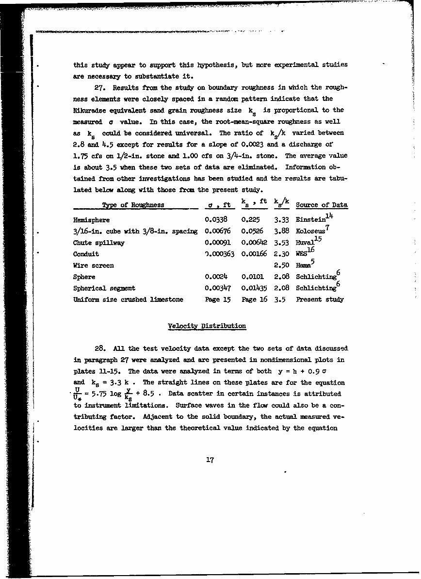
_27. Results from the study on boundary roughness in which the rough-

ness elements were closely spaced in a random pattern indicate that the

Nikuradse equivalent sand grain roughness size k is proportional to the

measured a value. In this case, the root-mean-square roughness as well

as k% could be considered universal. The ratio of k./k varied between

2.8 and 4.5 except for results for a slope of 0.0023 and a discharge of

1.75 cfs on 1/2-in. stone and 1.00 cfs on 3/4-in. stone. The average value

is about 3.5 when these two sets of data are eliminated. Information ob-

tained from other investigations has been studied and the results are tabu-

lated below along with those fron the present study.i k ,k t k/k

Type of Roughness a 2 f , ft /k Source of Data

Hemisphere 0.0338 0.225 3.33 EinsteinI1

3/16-in. cube with 3/8-in. spacing 0.00676 0.0526 3.88 Koloseus 7

Chute spillway 0.00091 0.00642 3.53 Huval 1 5

Conduit oo000363 000166 2.30 WES 16

Wire screen 2.50 Hama

6Sphere 0.002 0.0101 2.08 Schlichting

Spherical segment 0.00347 0.01435 2.08 schlichting

Uniform size crushed limestone Page 15 Page 16 3.5 Present study

Velocity Distribution

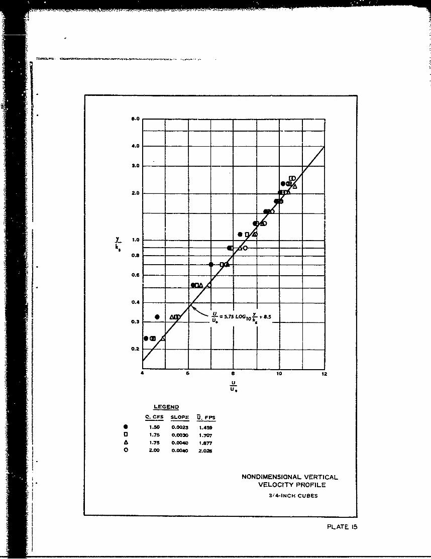
28. All the test velocity data except the two sets of data discussed

in paragraph 27 were analyzed and are presented in nondimensional plots in

plates 1-15. The data were analyzed in terms of both y = h + 0.9 aand k. = 3-3 k . The straight lines on these plates are for the equationU = 5.75 log - + 8.5 • Data scatter in certain instances is attributedU.I IIto instrument limitations. Surface waves in the flow could also be a con-

tributing factor. Adjacent to the solid boundary, the actual measured ve-

locities are larger than the theoretical value indicated by the equation

17

5.75 log - + 8.5 . Detailed study of velocity distributiofi close toU* k sthe boundary surface would be desirable.

Resistance Coefficients

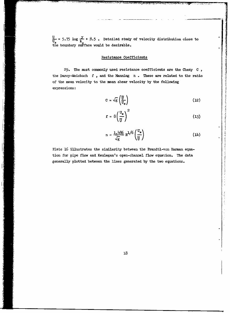
29. The most commonly used resistance coefficients are the Chezy C ,

the Darcy-Weisbach f , and the Manning n . These are related to the ratio

of the mean velocity to the mean shear velocity by the following

expressions:

Sr(2)

f 8((*)2f=8(~)(13)

1. = R/6-. / I (lki.)

Plate 16 illustrates the similarity between the Prandtl-von Karman equa-

tion for pipe flow and Keulegan's open-channel flow equazion. The data

generally plotted between the lines generated by the two equations.

18

PART V: CONCLUSIONS AND COMMENTS

30. The following conclusions, and comments thereon, were drawn from

the study:

a. The characteristic velocity distribution for two-dimensional channel flow at relative roughness d/k of8 or more a pears to be universal. The semiempiricalformula U/U, = 5.75 log y/ks + 8.5 can be applied exceptfor velocities very close to the boundary where the actualvelocity is greater than the theoretical value.

b. The root-mean-square value a of rough surface protru-sions is related to the Nikuradse roughness height k.and can also be treated as a roughness parameter forboundaries formed by uniform size roughness elementsclosely spaced in a random pattern. The condition shouldbe limited to cases in which the boundary is hydrodynami-cally rough. This conclusion should not be applied toboundaries that are classified as hydrodynamically wavy.

c. The location of the theoretical flow boundary beneath thetop of roughness protrusions does not appear to be con-stant. The datum for the boundary roughness in which thest.-ne layer thickness was more than one diameter is locatedat a distance of about 0.9 to 1.0 a . The distance wasclose to the mean stone diameter for the roughness thatwas only one layer thick. Additional tests are necessaryto evaluate the effect the interstices in the multilayerroughness might have on the location of the theoreticalflow boundary.

d. The characteristic velocity distribution appears to beindependent of absolute size and shape of the uniformlygraded material constituting the boundary roughness andof the bed slope, discharge, and flow depth.

e. The present study was limited to boundary roughnesses re-sulting with essentially uniform size roughness elements.The test results indicate that the relation between kand a is independent of the stone size and geometry aslong as the roughness elements are continuous and placed-in a random manner. The effect of stone gradation such asthat used for riprap is recommended for a future study.

Si19S I -

LITERATURE CITED

1. Keulegan, G. H., "Laws of Turbulent Flow in Open Channels," ResearchPaper RPU5Il, pp 707-741, Dec 1938, National Bureau of Standards,Washington, D. C.

2. Bazin, H., "Recherches Hydrauliques," Mem. divers savants, Sci. Math.et Phys., 19, Paris, 1865.

3. Powell, R. W., "Resistance to Flow in Rough Channels," Transactions.American Geophysical Union, Vol 31, No. 4., Aug 1950, pp 575-52.

4. Robinson, A. R. and Albertson, M. L., "Artificial Roughness Standardfor Open Channels," Transactions, American Geophysicil Union, Vol 33,No. 6, Dec 1952, pp 881--88T.

5. Hama, F. R., "Boundary-Layer Characteristics for Smooth and Rough Sur-faces," Transactions, Society of Naval Architects and Marine Engineers,Vol 62, 1954, pp 333-356.

6. Schlichting, H., "Experimenta. Investigation of the Problem of SurfaceRoughness," Technical Memorandum No. 823, Apr 1937, National AdvisoryCommittee for Aeronautics, Washington, D. C.

7. Koloseus, H. J. and Davidian, J., "Roughness-Concentration Effects onFlow over Hydrodynamically Rough Surfaces," Geological Survey Water-Supply Paper 1592-D, 1966, U. S. Geological Survey, Washington, D. C.

8. Brown, B. J., "Vertical Velocity Distribution in Streams," Interim

Report, Director's In-House Laboratory Research Program - Item L,Apr 1966, U. S. Army Engineer Waterways Experiment Station, CE,Vicksburg, Miss.

9. Chu, Y. H., '"oundary Effects of Turbulent Natural Channels," SecondInterim Report, Director's In-House Laboratory Research Program -Item L, Jan 1967, U. S. Army Engineer Waterways Experiment Station,CE, Vicksburg, Miss.

10. Chu, Y. H., "Boundary Effects of Turbulent Natural Channels," ThirdInterim Report, Director's In-House Laboratory Research Program -Item L, Nov 1967, U. S. Army Engineer Waterways Experiment Station,CE, Vicksburg, Miss.

Ii. McNown, J. S. and Malaika, J., "Effects of Particle Shape on SettlingVelocity at Low Reynolds Numbers," Transactions, American GeophysicalUnion, Vol 31, No. 1, Feb 1950, pp 74-82.

12. Hallmark, D. E. and Smith, G. L., "Stability of Channels by Armor-plating," Journal, Waterways and Harbors Division, American Societyof Civil Engineers, Vol 91, Aug 1965, pp i17-135.

13. Morris, H. M., Jr., "Flow in Rough Conduits," Transactions, American

Society of Civil Engineers, Vol 120, Paper No. 2745, 1955, pP 373-398.

14. Einstein, H. A. and El-Samni, E. A., "Hydrodyuamic Forces on a RoughWall," Reviews of Modern Physics, Vol 21, No. 3, July 1949, PP 520-524.

20

I~ I

1.15. Huval., C. J.j, "Flow in Chute Spillway at Fort Randall Dam.," TechnicalReport No. 2-716, Apr 1966, U. S. Army Engineer Waterways Experiment

-!Station, CE, Vicksburg, Miss.

16. Huval, C. J., "Prototype Hydraulic Tests of Flood-Control Conduit, EnidDam, Yocona River, Mississippi," Technical Report No. 2-510, June 1959,U. S. Armny Engineer Waterways Fxperiment Station, CE, Vicksburg, Miss.

|I.__21

11-'

1.4-• I

1.2

a-. _-- .-u-a.

1.,[.0V 2 10

i•,• 0.6-Ii0.4- - - -

0.2 .

0.00 0.01 0.02 0.03 0.04 0.05 0.06 0.07

DIFFERENTIAL HEAC.. FT

CALIBRATION CURVE

5/ ¶6-INCH PITOT TUBESLOPING MANOMETER

- •w;iI AEROSOL

I FPLATE I

I .2

r

0.6 -_ I0.5 1.41 1.43 1.35 1.40 1.42

0.4 1.43 1.40 1.37 1.4" 1.45

y.. FT 0.3 1.41 1.39 1.35 1.35 1.44

0.2 1.40 1.41 1.38 1.41 1.41

0.1 1.41 1.45 1.43 1.44 1.44

i I0 5 10 15 20 25 30

DISTANCE. IN.

DISTRIBUTION IN FLUME ENTRANCESTATION 04000 Q=1.80 CFS

0.3 - -

1.15 1.14

1,.2 1.11 1.12 1.11 1.10 1.12

y,. FT 1.06 1.08 1.0S 1.05 1.07

0.1 0.97 1.00 0.95 0.94 0.9S

0.85 0.89 0.91 0.80 0.82

"00 - I I I I a

50 10 15 20 25 30

DISTANCE. IN.

DISTRIBUTION AT TEST STATION 0+38.5

Q = 0.75 CFS

NOTE: ALL VELOCITIES ARE IN FEETPER SECOND. y- IS THE DISTANCE TYPICAL TRANSVERSEFROM THE TOP OF THE STONE.

SCALE DISTORTION. 3.13 VERTICAL VELOCITY DISTRIBUTIONSTO 1.0 HORIZONTAL. 3/4-INCH STONE

PLATE 2

II

*1.

30

I-

IIIlo-

IL 1j

0 F

Z I II a I.IJ

0.007 0.009 0.011 0.013 0.015 0.017

.STONE DIAMETER. FT

•3 •

0 20

-1aII •

20I

IL0

I

I-

10-

S•0.2 0.4 0.6 o.e 1.0 1.2

S ! SHAPE FACTOR

STONE CHARACTERISTICS

NOMINAL STONE SIZE = 1/8 INCH100 SAMPLES

PLATE 3

K I

020

0 20-

0

U.

I-z

10-

0.50 0.60 0.70 0.80 0.90

STONE OIAMETER. IN.

a 20-I

0

0I-

zUp 10-

b t 0 I ..IL

0 - ! I I iI IS0.20 0.40 0.60 0.60 1.00

SHAPE FACTOR

STONE CHARACTERISTICS

NOMINAL STONE SIZE = 1/2 INCH

100 SAMPLES

PLATE 4

J I

1- 20 -

U.

S0 I

10

IL~

0-I

• • o

I"L I •, II I

0.4W0 0.595 0.705 0.814 0.923 1.032 1.141 1.250

STONE DIAMETER, IN.

* 30 -

I-

0

20

U.

O I•

~ 0I'_

0.

0.118 0.218 0.317 0.418 0.518 0.615 0.714 0.814

SHAPE FACTOR

STONE CHARACTERISTICS

NOMINAL STONE SIZE = 3/4 INCH4100SAPE

PLATE 5

30j

-0 I

4

Ii • - I

o 10o• I I I

STON DIMTR IN.

I-

S IA

10I

III I

0- - -

I..!....I. II I

I lu -0 Ii iI

000 SAPE

i-i 6i

"I I I I- IIII

10 10PF-

STON CHRACERITIC

I

0I0

0 0.I•

1 /8 INCH STONE

1/2- INCH STONE

]i l

v._.._ , 3/4- INCH STONE

T

0.0 0ZFT

II INH IN

3/4- INCH CUTI

STONE HORZONTAL MEASUREMENT

STONE SIZE. IN. INCREMENT, Im. D0 SIZE. FT 0. FT

1/8 0.12 0.01036 000361/2 030 0055 001483/4 0.30 0 .00 00181SI

0.30 0 .106 0.02721- 3/4 CJSE 0.30 0.0S3 0.0236

ROUGHNESS SURFACE PROFILE

PLATE 7

I•

1.010.9 A __

0.S_ - -

a aUMAX0

0 0

0.7A

o0 70 so 9010

ii

PERCENTAGE OF TOTAL DATA POINTS

LEGEND NOTE: 0 4ROOT-MEAN-SQUARE VALUE__________ __________ _________________WITH SPECIFIED PERCENT-

STONE TOTAL NO. AGE OF POINTS OMITTEDSYMSOL SIZE. IN. DATA POINTS ROOT-MEAN-SQUARE VALUETO INCLUDE ALL THE DATA

0 1/8 900 POINTSA 1/2 814

* 3/4 7S9

0 1 836

13 3/4 CU BE 72

ROOT-MEAN-SQUARE ANALYSIS

P1ATE 8

Al

S...~. - .~tl. - mI . .. .. • • • c L

|1.I.* *1-

FLOW ?

WATER SURFACE

U

yh

"* THEORETICAL FLOW TOP OF STONE SURFACE

BOTTOM OF STEEL FLUME

LEGEND

-| -k=2a

X =POINT GAGE READINGON STONE SURFACE

; •N - NUMBER OF READINGS

DEFINITION SKETCHi- OF PARAMETERS

PLATE 9

70-

40 30U,/

1 * 035 -0.10 0.067SLOPE 5 - =0.00675=

10

4--,'425

,o

"" 0.1 0.2 0.3 0.4 0.S

h. FT

BASIC EQUAT:UN:

30 k0.4 u\

ks =•30 x .00675 =0.206 FT ks ANDSAMPLE COMPUTATION

f= 4.25 x 0.00675 0.0287 FT ESCOFFIER METHOD

Q = 2.50 CFS, S. = 0.004

I-INCH STONE

PLATE 10

4.I"

-AID

200. 0 - --O

am -

0.804.0-

10 1.0 1- 0--

L)00

20 0. - -.02 1.-509_

t.5 0.0o 1.2

iI I

10 _. .0040 2.7 09

i 0.6 -.. - .-

.: ~. Q~GE~j ~NONDIMENSIONAL VERTICAL

1/S-INCH STONE

PLATE 11

I

4.0 --

3.0 .0

0 0 ,

2.0

0• v

* A

Ic 0 .6 1,

U,_0.6

0.2

0.1

4 6 8 10 12

u

LEGEND

Q. CPS SLOPE U. FPS

9 1.25 0.0023 1.46

* 1.75 0.0040 1.920 1.75 0.0060 2.46

NONDIMENSIONAL

VERTICAL VELOCITY PROFILE1/2-INCH STONE

PLATE 12

6.0 i ,4.03.

El 1 'K I

2.0 - , -

= . _ _5.75 LOG__ + 8.5

4. .0l A- 11.0 .1 1 4

0.6 E

0.4

~E1

0.6 A 0

IiI-I -

4 6 10 12

U,

LEGEND

Q. CFS SLOPE 0, FPS

V 1.50 0.0023 1.59

0 1.75 0.0040 2.03

-0 ?2.00 0.0060 2.31

NONDIMENSIONAL VERTICALVELOCITY PROFILE

3/4-INCH STONE

PLATE 13

4.0 - - - - - -

3.0 J_ _

tn 02.0

1.0 -

0.8 i - -

0.4 -

,_ • ~0.3-

-H__ - =5.75 LOG/0 +8.5UEE °'J i __T.0.2

4 6 a t0 12

U,

LEGEND

Q. CFS SLOPE U. FPS

0 1.50 0.0023 I-500 1.75 0.0023 1.63

(3 2.00 0.0023 1.692.00o 0.0040 2.02

A 2.so 0.0040 2.22A 2.50 0.0060 2.66

NONDIMENSIONALVERTICAL VELOCITY PROFILE

~ 1-INCH STONE

PLATE 14

I

2.0 - -

II

"2 6.0

'1: .4. ...I.1 ___ !5.7S LOG, 0 .. 8.5j ~~0.3 __-

S0.24 6 810 12

Im U

LEGEND

Q. CFS SLOPE FPS

0 1.50 0.0023 1.4591.75 0.0030 1.707

a 1.75 0.0040 0770 2.00 0.0040 2.026

NONDIMENSIONAL VERTICALVELOCITY PROFILE

* I 4-INCH CUBES

PLT I15

-Ii iI PL TE1

-i u,

-l .1

20.0

15.0 -_o1

C 32.i LOG10 (!?Zd

10.0 --

9.0 _ - -- _ _

8.0

7.01___

6.0 -d

k.5.0 - 4--

4.0-/

3.0 - -o

0 C=32.I LOG 10

2.0I I I

NOTE: d = CORRECTED FLOW DEPTH

R = HYDRAULIC RADIUS = d FOR

TWO-DIMENSIONAL FLOW

40 so 60 70 s0

CHEZY'S C

LEGEND

A 1/8-INCH STONE

A1/2-INCH STONE

0 3/4-INCH STONE

0 I-INCH STONE

* 3/4-INCH CUBE

RESISTANCE COEFFICIENTS

PLATE 16

I

• •APFENDfl A: TEST DXAA

N

°I

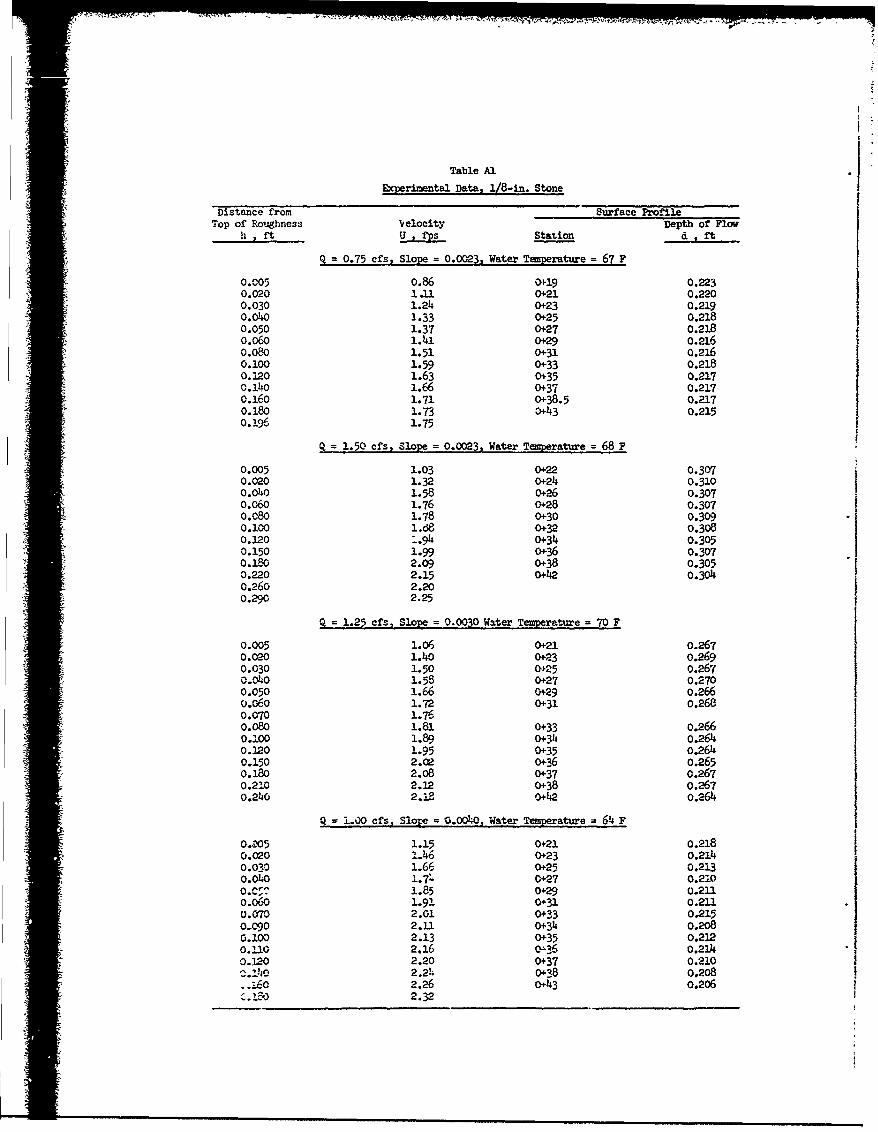
Table AlExperinental Dataý i/8-in. Stone

Distance from Surface ProfileTop of Roughness Velocity Depth of Flow

h ,ft u , Station d ft

Q 0.75 cfs, Slope = 0.0023. Water Tapperature = 67 F

0.005 0.86 0+19 0.2230.020 1.11 0+21 0.2200.030 1.24 0+23 0.2190.0o4O 1.33 0+25 0.2180.050 1.37 0+27 0.218o.o6o 1.41 0+29 o.2160.080 1.51 0+31 0.2160.100 1.59 0+33 0.2180.320 1.63 0+35 0.2170.16O 1.66 0+37 0.217o.16o 1.71 0+38.5 o.217O.180 1.73 0+43 0.2150.196 1.75

Q 1.50 cfs, Slope = 0.0023, Water Temperature = 68 F

0.005 1.03 0+22 0.3070.020 1.32 0+24 0.310o.o~o 1.58 0+26 o.3070.06O 1.76 0+28 0.3070.080 1.78 0+30 0.3090.100 1.68 0+32 0.3080.120 ..94 0+34 0.3050.150 1.99 0+36 0.3070.180 2.09 0+38 0.3050.220 2.15 0+42 O.30o40.260 2.200.290 2.25

Q= 1.25 cfs, Slope = 0.0030 Water Temperature = 70 F

0.005 1.06 0+21 0.2670.020 1.40 0+23 0.2690.030 1.50 O+25 0.2670.040 1.58 0+27 0.2700.050 1.66 0+29 0.2660.06o 1.72 0+31 0.2680.070 1.760.080 1.81 0+33 0.2660.IO0 1.89 0+34 0.2640.120 1.95 0+35 0.2640.150 2.02 0+36 0.2650.180 2.08 0+37 0.2670.210 2.12 0+38 0.2670.240 2.18 0+42 0.26d

= .,00 cfs Slope = 1.004-0, Water Temperature 64 F

0.W05 1.15 0+21 0.2180.020 1.46 0+23 0.2140.030 1.66 0+25 0.2130.040 1.7. 0+27 0.21oo... 1.85 0+29 0.211o.06o 1.91 0+31 0.2110.070 2.01 0+33 0.2150o090 2.11 0+34 0.2080.100 2.13 0+35 0.2.120.110 2.16 0ý36 0.2140.120 2.20 0+37 0.210

2.24 0+38 0,208-160 2.26 0+43 0.206

.1,04 2.32

Table A2

Experimental Data, 1/2-in. Stone

* Distance from SUMwace ProfileTop of Roughness Velocity Depth of Flow

h x ft U I fps Station - d , ft

= 1,25 ofs, Slope = 0.0023, Water Temperatfwe = 83 F

0.020 0.90 0422 0.3300.050 1A9 0+24 0.3300.080 1.28 0+26 o.3260.110 1.38 0+28 0.325o.140 1.47 0+30 0.3230.170 1.58 0+32 0.3250,200 1.63 0+34 0.3260.230 1.67 0+36 0.3240.260 1.73 0+38 0.3240.290 1.77 0+41 0.3230.310 1.81 o44 0.322

0+45 0.320

,= 1.75 cfs, Slope = 0.0023, Water Temperature = 85 F

0.020 0.96 0+22 o. 4290.050 1.22 0+24 0.4290.080 1.33 o+26 0.4290.110 1.45 0+28 o.4280.1.0 1.52 0+30 o.4280.170 1.61 0+32 0.429

* 0.200 1.64 0+34 o.4310.240 1.69 0+36 0.4300.28o 1.75 0+38 0.14300.320 1.82 0+41 o.4310.360 1.87 0+43 0.4a29

Q 1.75 cfs. Slope = 0.001.0, Water Temerature =85F;o.o16 1.4o 0+22 0.343

0.030 1.46 o+24 0.-44O.060 1.64 0+26 0.344S0.o9o 1.78 0+28 0.3420.120 1.89 0+30 0.3390.150 1.99 C+32 0.3420.180 2.07 0+34 o.31i60.210 2.16 0+36 0.3450.214o 2.26 0+38 0.3440.270 2.33 0+41 0.3460.300 2.38 0+43 0.30.330 2.38 0+45 0.343

= 2.00 cfs. Slome = 0.0060, Water Temperature 68 F

0.030 1.77 0+22 0.3100.06o 2.03 0+24 0.3080.090 2.25 0+26 0.3000.120 2.41 0+28 0.3010.150 2.54 0+30 0.2990.180 2.64 0+32 0.303

0.210 2.74 0+34 0.3100.240• 2.79 0+36 0.3000.270 2.86 0+38 0.300

o+41 0.2930+43 0.3970+45 0.395

Table A3

Experimental Data, 3/4-in. Stone

Distanve from Surface PriofileTop of Roughness Velocity Depth of Flow

h U , fps Station d Pt

Q= 1.00 cfa. Slope = 0.0023, Water Temperature = 78 F

0.015 0.88 0+22 0.3240 .020 0.92 0+24 o.3240.030 0.99 0+26 0.323o.o4o 1.01 0+28 0.3240.050 1.05 0+30 0.325o.06o 1.08 0+32 o.3240.070 1.10 0+34 0.3220.080 1.14 0+36 0.3230.100 1.20 0+38 0.3230.120 1.28 0+40 0.3230 .140 1.32 0+42 0.322o.16o 1.35 0+44 0.3290.180 1.390.200 1.420.220 1.440.250 1.1490.280 1.530.305 1.55

SQ 1.50 crs. Slope = 0.0023. Water Temperature 76 F

0.020 1.O4 0+22 O.384Ox40 1.316 0+24 0.3810.060 1.30 0+26 0.3810.080 1.44 0o28 0.3790.100 1.47 0+30 0.3780 0120 1.54 0+32 0.3780.150 1.61 0+34 0.3780.180 1.70 0+36 0.3770.210 1.73 0+38 0.3760.24o 1.80 o+41 0.3750.270 1.4 00A3 0.3770.300 1.86 0+45 0.3690.330 1.9 go0.360 1.93

Q = 1.75 cfs. Slope = 0.0040. Water Temperature = 73 F

0.010 1.19 0+22 0.3580.020 1.34 0+24 0.3510.030 1.45 0+26 0.358O.O4•0 1.53 0+28 0.3560.050 1.58 0+30 0.3500.o6O 1.67 0+32 0.351"O.00 1-.7C 0+34 0.3600.100 1.84 0+36 0.3520.120 1.95 0+38 0.352o.150 ?.07 0+41 0.3500.180 2.12 0o+43 0.3550.210 2.20 0+45 0.3370.240 2.270.270 2.340.300 2.380.330 2.41

= 2.00 ct. Slope = 0.0060. Water Temperature = 76 F

o.o0o 1.40 0+22 0.3663.030 1.55 0+24 0.379o.oGo 1.,7 0426 0.376o.C 0 1.8 6 0+28 0.366

0.C4A0 2.05 0+30 0.3820.100 2.13 0ý32 0.3740.12-0 2.21 0+34 0.3670.150 2..4 0+36 o.3660.1" 2.!Z 0.33 0.360

.210 2.ý2 0+4i 0.36200.3 0. 3%

.. "O 2."7

=I i

Table A.

Fxperimental Data. I-in. Stone

Distanc.e frolm Surface Profilem Top of Rovemess Velocity Depth or Flow

Q 1.50 cf., Slope 0.0023 Water Tenperature - 7U F

0.016 0.92 0.22 0.3790.036 1.00 0o23 0.3620.066 1.15 0+25 0.3790.096 1.25 0+27 0.3790.146 1.41 0+29 0.3790.196 1.54 0+31 0.o80

:M0.22 1.66 0433 0.380o.296 1o-r. 0+35 0.380vo.346 1.83 0+37 0.380

0.241 0.380010.3 0.3800.A5 0.381

Q - 1.75 efs, Slope 0.03., Water Temperature - 72 F0o.o6 1.00 0+21 0.41t

0.036 1.13 0+23 0.4200.066 1.29 0+25 0,1117o.o96 1.36 0-27 0.4180.14.6 1.54 0.429 0.416y0.196 1.67 0+31 0.4180.246 1.78 0+33 0.4170-296 1.87 0+35 o.4180.32.6 1.98 0+37 0.417o.396 2.01 0.o41 0.415

0+43 o.41ý0.45 0.41,

2.00 efs. Sloee 0.0023. 'dater Temperature - 74 F

0.016 1.00 G-21 o.VC0.036 1.19 0-23 0.470-0.08 1.31 0+25 0.468I o.096 1.40 0+27 0.470

o0.146 1.57 0+29 0.470o.196 1.73 0,31 0.470o.246 1.8 0+33 0.472

"1.296" .e7 0+35 o.47oo.346 1.92 0+37 0.4700.396 1.98 o. o.069

o.4426 1.98 0+43 0.4700+45 0.469

Q - 2.00 cfs, Slope o.oo40, Water Temperatu.e - 76 F

0.016 1.21 0-21 0.38L0.036 1.43 0-23 ,.3910.o66 1.66 025 0.389o.o9 1.75 0-27 0.392o.14 1.9h 0+29 0.393o.19 2.11 0+31 0.3900.246 2.25 0+33 0.390

2.2 2.36 0+35 0.3870.346 2.39 0+37 0.386

0+35.5 r. 3, 00+41 0.o.680.43 0.3890-45 0.385

Q - 2.50 efs Slope 0.0040. War Te-r erature -77 F

o.o16 1.38 0+22 0.4650.036 1.53 0.24 0.463o.066 1.70 0+-6 o.430.096 1.8- ,o,- o.463o.146 2.06 0.30 0.465o.!96 2.23 0.32 O.46..0.2k6 2.33 O.34 " 0.4640.296 2.44 0.36 0.!.0.346 2.53 0+38 ..0.396 2.61 0+41 0.4

0.45 0.4ý,0 2.50 cf,. Sic;e * 0.0060. Water 7-e= ratr.-e - 78 F

0.016 1.68 0+221.816 o.024 .

0.0C6 2.06 0-2t C.L.0.096 2.14 0-2P C.L-70 .146 2.45 0.4090.196 2.EP ".4100.246 2.9$ O..-0.0.296 3.0>6 0-3 0.41-.0.346 3.1- 0.8s 0.419

0.43 0.414O-, '.410

I

£- - --

"Table A5

Experimental Data, 3/4-in. Concrete Cubes

Distance f'rom Surface ProfileTop of Roughness Velocity Depth of Flow

h , ft U, ps Station d ft

Q = 1.50 cfs, Slope 0.0023, Water Temperature = 85 F

0.016 0.72 0+19 0.3850.030 0.81 0+21 0.3820.060 1.08 0+22 0.3830.090 1.22 0+23 0.3840.120 1.36 0+24 0.3830.150 1.44 0+25 0.3840,180 1.55 0+26 0.3840.220 1.63 0+27 0.3830.260 1.71 0+28 0.3830.300 1.74 0+29 0.3820.340 1.76 0+30 0.380

0+31 0.382

Q= 1.75 cfs, Slope= 0.0030, Water Temperature 87 F

0.016 0.88 0+19 0.3820.030 1.08 0+22 0.3800.060 1.26 0+23 0.3820.0)0 1.48 0+24 0.3820.120 1.56 0+25 0.3820.150 1.70 0+26 0.3820.180 1.77 0+27 0.3820.220 1.86 0+28 0.3810.260 1.94 0+29 0.3820.300 2.00 0+30 0.3800.3ho 2.060.370 2.06

Q = 1.75 cfs, Slope = 0.0040, Water Temperature = 86 F0.016 1.06 0+19 0.349

0.030 1.16 0+22 0.349 i0.060 1.43 0+23 0.3510.090 1.68 0+24 0.3490.120 1.8o 0+25 o.3480.150 1.94 0+26 0.348O.180 2.02 0+27 0.3470.220 2.09, 0+28 0.3460 260 2.19 0+29 0.3470.300 2.28 0+30 0.3450.330 2.33

Q = 2.00 cfs, Slope 0.0040, Water Temperature = 7j F

O.016 1.00 Oi18 0.3850.030 1.27 0+19 0.3820.0o60 1.58 0+20 0.3820.090 1.75 0+21 0.3800.120 1.94 0+22 0.3820.150 2.03 0+23 0.38140.180 2.13 o+2-4 0.3840.220 2.20 0+25 0.3840.260 2.30 0+26 0.3840.3A0 2.34 0+-27 0.3840.130 2.38 0+28 0.3320.370 2.42 03+0 0.3840430 0. 381

0o31 0.381

4

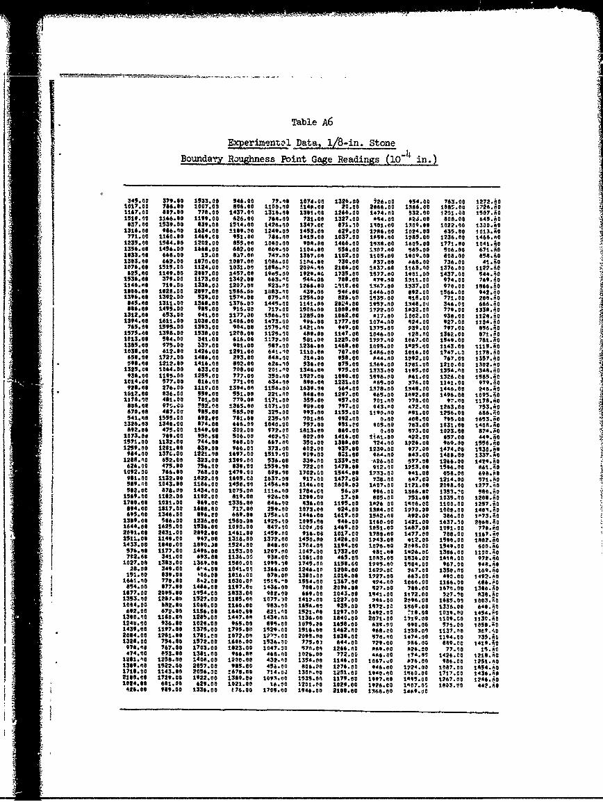
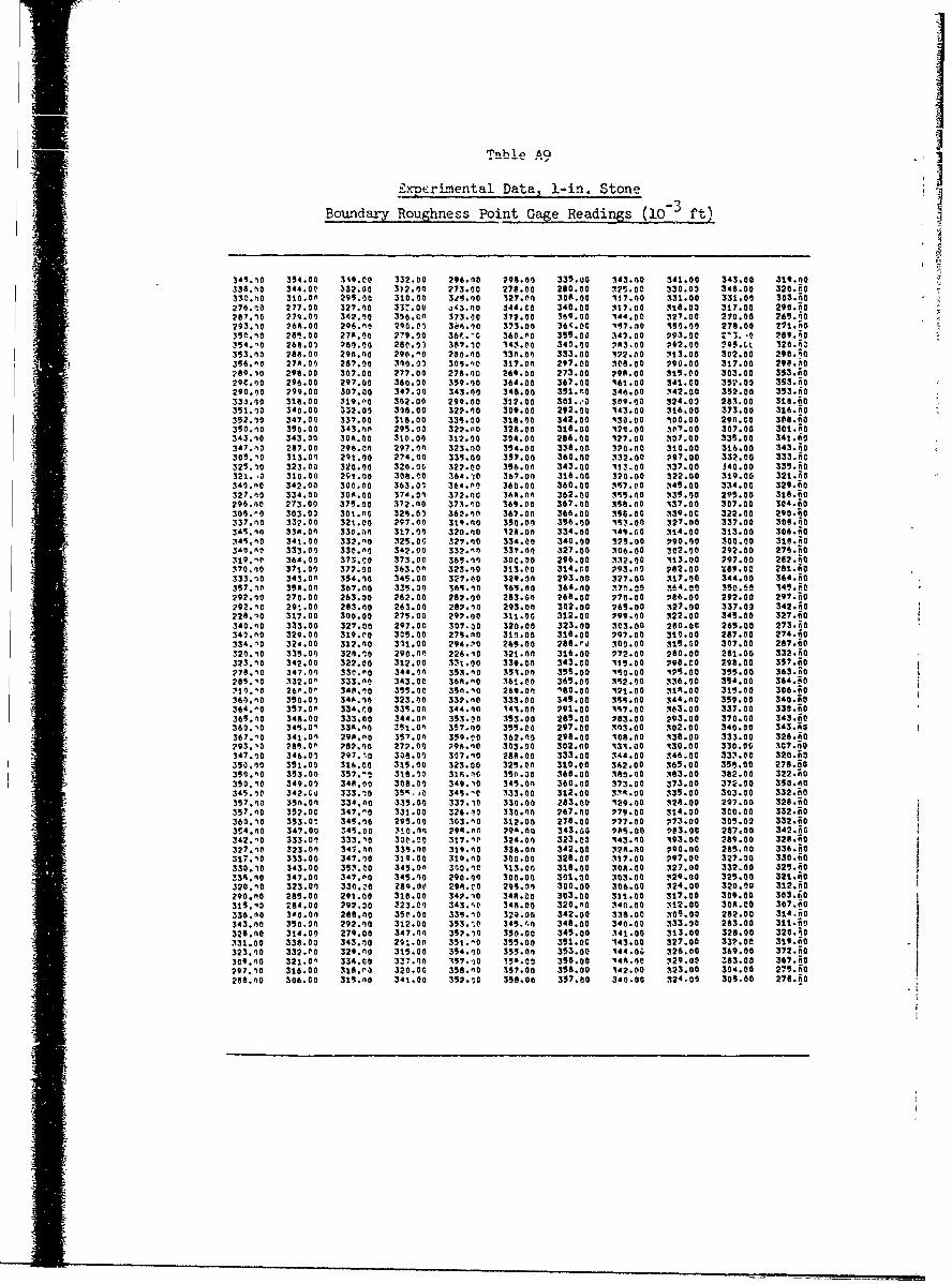
,| IITable A6

Eperimentcl Data, 1/8-in. Stone

Bounda'ry Roughness Point Gage Readings (10- in.)

345.00 379.00 1533.00 946.00 77.,o 1074.00 1326.00 126.00 954.00 763.00 1272.A01017.00 746.00 1007.05 606.00 1100,00 1140.00 20.00 2066.00 1386.00 0ee.O00 1726.nO1167.00 817.00 77M.00 1437.00 1316.00 1301.00 1266.00 1474.n0 532.00 1201.50 1507.001510.90 1166.00 1199.00 626.00 760.00 731.00 1327.00 A04.00 P23.00 008.00 645.A0937.00 1539.00 839.06 1514.00 1426.00 1347.00 871.10 1101.00 1309.00 1022.00 1300.00

1316.00 9660.0 16.06 1.00 7.0 1413.00 619370 1786.00 1024.00 635.00 1016.00771.00 1190.00 14691.0 1 00 124.A0 1453.00 1037.00 1096.00 1062.00 1236.00 1466.n0

1235.00 1564.00 1202.00 605.00 1060.00 904.00 1466.00 1138.00 1605.00 1771.00 1041.A01356.00 1456.00 1668.00 662.00 069.00 1104.00 556.00 1307.00 565.00 506.00 671.A01633.00 668.00 19.00 637.00 747.00 1367.00 1102.00 1109.00 1909.00 608.00 895.n01303.00 662.00 1070.00 1087.00 1086.00 1In4.00 730.00 P37.00 468.00 736.00 41.io1076.00 1515.00 1124.00 1031.00 1806.00 2094.00 2106.00 1837.00 1169.00 1376.00 1122.00625.00 1149.00 2007.00 1457.00 1905.00 1929.nG 1735.00 1577.00 1901.00 1437.00 544.40

1536.00 379.00 1173.00 1342.00 663."0 548.00 700.00 479.90 1311.00 974.00 769.401146.06 719.00 1336.03 1207.00 523.00 1266.00 Z1.0.00 1347.00 1337.00 970.00 1666.001806.00 1828.00 2097.00 1956.00 1803.00 439.00 540,00 1446.00 092.00 1566.00 942.n01396.00 1392.00 539.00 1574.00 875.n0 1296.00 826.00 1035.00 416.00 771.00 200.00

845.00 1311.00 1366.00 1376.09 1449.00 1141.00 2024.00 1957.00 134$.0O 346.00 666.000866.00 1495.00 965.00 916.00 717.00 1506.00 1000.00 1722.00 1032.00 779.00 13368.0

1312.00 693.00 941.00 1177.00 1566.00 1289.00 1062.00 417.00 1002.00 938.00 1126.001394.00 1611.00 1036.00 1406.00 1473.60 496.00 1777.00 1074.A0 424.00 927.00 1104.00765.00 1595.00 1393.00 904.00 1579.00 1421.00 949.00 1375.00 239.00 797.00 656.00

1575.00 1398.00 1538.00 1290.00 1125.00 489.00 1147.00 1046.00 128.00 1362.00 67I.Ao1013.00 504.00 341.00 616.00 1172.00 581.00 1225.00 1727.00 1067.00 1949.00 761.001385.00 975.00 137.00 901.00 567.00 1236.00 1466.00 1095.00 1425.00 1143.00 1119.001036.00 612.00 1426.00 1291.00 641.40 1110.00 707.00 1406.00 1016.00 1747.L0 1176.60

650.00 1721.00 1466.00 293.00 840.00 314,00 958.00 P44.40 1292.00 767.00 1357.nO590.00 1212.00 1416.00 602.00 626.10 936.00 875.00 1369.00 1201.00 1210.00 1302.00

132:5.06 1064.00 633.0 706.00 201.'0 1346.00 979.00 1333.00 1199.00 1354.00 1346.AO936.0 0 15 125.00 777.00 350.00 1927.00 1090.00 1596.00 061.00 1326.00 1565.n0

1014.00 577.00 016.00 771.00 634.00 690.00 1231.00 46s.00 376.00 1141.00 979.60926.00 276.00 1119.00 1394.00 1156.00 1639.00 664.00 1376.00 1346.00 1446.00 246.00

1012.00 $36.00 959.00 551.00 221.00 646.00 1297.00 065.00 10f92.00 1496.00 1095.;01176.10 461.00 701.00 ?79.00 1171.00 359.00 957.00 701.00 770.00 91.00 1176,.0806.06 97S."0 !00.41 1365.00 1071.90 999,00 797.00 943.00 472.00 1263.00 753.60670.00 487.00 905.00 565.00 3259.00 993.00 1155.00 1190.00 P91.00 1256.00 666.Fo541.00 1555.00 692.00 761.00 235.00 901.00 992.00 0.00 406.00 795.00 1653.;0

1326:08 1340.00 874.00 666.00 1040.00 757.00 951.00 405.00 703.00 1031.00 1406.AD0092.00 475.00 1049.00 302.00 972.00 1613.00 860.00 0.00 573.00 1023.00 074.00

1073.00 709.00 95M.00 506.00 40P.09 802.00 1416.00 1441.00 422.00 657.00 440.601571.00 1132.00 744.00 960.60 667.00 350.00 1306.00 124.00 1226.00 969.00 1556.001259.00 1201.00 639.00 966.00 373.00 602.00 939.00 1239.00 977.00 1474.00 1130:60

964.00 1376.00 1221.00 1697.00 1517.00 909.00 U;1.00 464.00 043.00 1486.00 1337.001206.,0 652.00 323.00 1399.00 536.00 339.00 1339.00 026.00 577.00 1266.00 1429.50626.00 475.00 756.00 039.00 1559.90 722.00 1478.00 912.00 1253.00 1596.00 661.40

1092.00 766.00 768.00 1479.00 699.10 1702.00 1544.00 1233.00 941.00 650.00 69S."0961.00 1132.00 1622.00 1605.00 1637.00 917.00 1477.0a 736.00 647.03 1214.00 571.hD569.00 1043.00 1166.00 1450.00 1456.00 1146.00 1608.00 1407.00 1121.00 2006.00 1277.;0502.00 070 a.00 134.0 1075.001n 1110.00 1704.00 96.0p 996.00 1366.00 1353.'0 560.00

1569.00 1162.00 1102.00 019.00 926.00 1209.00 17.00 005.00 751.00 1035.00 1206.iO1700.00 1011.00 069.00 1336.00 046.40 636.00 1195.00 1426 00 1006.00 1100.00 1297.00094.00 1617.00 1600.00 717.00 259.00 1073.00 924.00 1384.0C 1270.00 1000.00 1401.90695.00 1346.00 696.00 669.00 1754.60 1446.00 1619.00 1502.00 092.00 306.00 1073.50

1369.06 506.00 1236.00 1560.00 1925.00 1095.00 946.00 1160.00 1421.00 1637.00 2040.A01644.00 1625.00 1536.00 1090.00 647.00 1004,00 1469.00 1051.00 1487.00 1091-00 770.602091.00 2031.00 2092.00 1461.00 1459.00 916.00 1017.00 1780.00 1477.00 700.00 1167.AQ1511.00 1149.00 947.00 1316.00 1372.00 1450.00 1426.00 1243.00 912.00 1190.00 1602.001433.00 1040.00 1090.30 1924.00 846.00 1704.00 1194.00 1026.00 2C96.00 1549.00 600.;0

576.00 1177.00 1496.00 1193.00 1207.90 1047.00 1732.00 961.00 1926.00 1306.00 1100.90792.00 341.00 693.00 1136.05 938.0' 1061.00 469.00 1003.00 1%36.00 1614.00 972.oO

1027.00 1363.00 1369.00 1500.00 1999.10 1749.00 1150.00 1295.00 1M04.00 967.00 946.0028.00 349.00 6",4.00 1041.00 1366.00 1246.00 1200.00 1622.00 267.00 1350.00 169.n0

191.00 039.00 '06.00 1016.00 876.00 1300.00 1016.00 1927.00 663.00 490.00 2492.001661.00 770.00 8,2.00 1030.00 151.-0 1554.00 1367.00 124.40 1066.00 1166.00 006.00

694.00 077.00 1460.00 1197.0u 1436.00 706.00 2096.00 527.00 706.00 1670.00 1386.501677.00 2095.00 1954.0 1633.00 960.00 469.00 1043.00 1041.00 1172.00 527.00 030.001353.00 1267.00 1527.00 1165.00 1077.10 1417.00 1227.00 296.00 2096.00 1605.00 1003.701004.00 062.00 1006.00 1166.00 983.00 1695.00 935.00 1172.00 1569.00 1336.00 64 .10

692.00 672.00 1156.00 1640.00 021.00 1521.00 1297.00 1492.00 tlS.00 1039.00 1494.i01300.00 1180.00 128b.00 1447.00 1439.00 1136.00 1640.00 2071.00 1719.00 1109.tC 113A.oO1240.00 936.00 1020.00 965.00 090.00 1075.00 1695.00 439.00 990.00 ?57.00 1056.401439.00 1197.00 1379.00 1795.00 1529.00 1516.00 1462.00 068.00 1330.09 1137.00 307.402034.00 1261.00 1761.00 1072.00f 127?.00 2099.00 1036.00 570.00 1474.00 1194.00 735.AG1326.00 754.00 1572.00 1606.00 1936.00 775.02 644.00 729.00 286.00 069.00 1419.O

970.00 767.00 1703.00 1623.00 1047.00 970.00 1260.00 049.00 026.00 77.00 vs.ic4?4.00 853.00 1361.00 966.00 468.n0 1026.00 772.00 446.00 174.00 1420.00 1210.oO

1261.10 1230.00 1400.00 1200.00 432.n0 1354.00 1146.00 1067.uO P76.00 986.00 1291.0O1309.00 1522.00 2057.00 965.00 456.00 806.p0 1276.00 946.00 1724.00 1087.00 1494.AO1716.00 1143.00 2056.90 :678.00 714.0, 130P.00 1251.00 1940.00 1060.00 1717.00 1436.302100.00 1729.00 1922.00 1389.00 103o00 1535.00 1179.00 1997.00 1095.00 1267.00 1246.601024.00 601.00 629.00 1021.00 14.00 1201.00 1009.00 1926.00 1007.00 1603.00 442.00

426.00 969.00 1336.00 176.00 1705.00 1946.00 2100.00 1366.00 1449.00

Table AY

E:coerimental Data, 1/2-in. Stone

lBoundary Roughness Point Gage Readings (10- rt)

266.10 257.00 259.00 240.00 279.00 ?48.nC 2'0.0O0 240.00 ?44.00 767.00 768.00

260.10 271.00 24n.00 28t.00 279.00 240.00 263.00 287.00 p62.00 261.00 263.00

271.110 26A.00 267.00 286.00 280.19 247.00 260.00 262.00 240.0: 265.n0 261.00

268.00 287.00 277.00 282.10 25A.10 241.00 200.nO 241.n0 248.00 241.00 248.0n

262.8 0 260.00 28W.00 279.00 267.00 261.10 249.00 243.00 265.00 243.00 240.10S287.00 250.00 243.00 272.00 271.oP 743.0n 251.o0 262.40 258.00 247.0' 279ýAO

279.00 262.00 265.00 ?63.00 25.00 252.0n 263.00 2-7.00 245.00 240.00 26S.;0

246.10 283.00 282.00 276.0n 267.00 271.O 273.00 2A6.10 277.00 246.00 250.00

248.00 276.00 274.00 261.00 262.I0 270.00 ?86.00 263.00 ?82.00 240.00 250.60

257.10 287.00 272.00 270.00 266.'0 26t.0n 274.00 270.0C 270.00 250.00 263.n0

250.10 Of 0 264.00 283.04 272.00 267.00 268.00 230.00 257.00 255.00 262.00

240.10 264.00 257.00 257.00 267.00 263.00 252.00 243.00 261.00 248.00 248.n0

?274.0 247.1)0 242.00 ?40.00 258.00 263.00 240.00 253.00 266.00 263.00 240.50

258.00 240.00 250.g0 249.01 243.ý0 259.C0 240.00 263.00 265.00 268.00 240.00

260.10 266.00 257.00 246.00 269.10 240.00 253.00 763.00 26.00 271.00 240.00

274.00 249.0J 271.00 242.0t 251.00 269.00 268.00 259.00 166.00 265.00 246.00

?32.00 261.00 240.00 257.00 241.00 270.00 267.00 260.00 256.00 263.00 272.00

"240.00 262.00 263.00 266.00 272.10 275.00 262.n0 244.'^ 263.00 270?.0o 266.00

240.10 263.00 262.n0 267.00 260.10 26R.00 25'.00 265.00 2'0.00 263.C0 261.0

240.10 240.00 270.00 259.00 250.40 277.00 279.00 261.00 261.00 250.00 253.;0

274.00 268.00 Z63.00 243.00 242.10 256.00 255.00 252.0n0 50.00 262.00 264.00

2278.0 240.00 266.00 257.00 272.00 274.00 275.00 267.00 :60.00 240.00 262.n0

252.00 263.00 274.00 279.00 246.00 260.00 272.00 974. 0 ?72.00 260.00 262.0

265.00 236.00 24P.0 259.00 242.00 240.n0 259.00 273.00 241.00 244.00 250.00

259.00 260.C0 253.00 260.00 25F.00 263.00 273.00 P63.00 261.00 240.00 250.!0

267.00 250.00 253.10 257.00 250. 0 P6. .0 265.00 >60.nO 273.00 240.00 259.50

255.00 249.00 277.00 272.00 262.10 282.00 253.00 266.00 270.10 264.00 254.60

247.00 260.00 256.00 256.00 264.10 270.00 267.00 PA0. I 240.00 263.00 243.00

272. 0 263.00 262.00 255.00 24r..0 263.0n 265.00 254.00 741.00 243.00 264.10

-67. 0 270.00 22'1.0O 261.00 ?7. 10 252.00 240.00 740.no 253.00 249.00 264.60

263.ý0 262.C0 253.00 243.00 277. 10 269.00 240.00 240.00 252.00 263.00 272.0024.0,0 240,.0O 263.n0 240.00 260.nO 280.0n 259.00 "4.0 . o 40.00 244.00 257,A0

240.00 260.00 24C.10 240.10 256.10 266.00 275.00 240.00 250. 00 245.00 250.40

260. 0 266.00 269.00 281.00 263.)0 265.00 27,.00 713.0O 288 .00 266.00 257.;0

297.10 286.00 262.00 260.0n 25A.10 273.00 24S.00 247.00 256.00 274.00 273.00

296.00 266.01 2!3.10 242.00 252.00 249.00 244.01 256.00 P86.00 264.00 252.00

258.10 208.00 257.10 252.00 250."0 253.00 261.00 P72.00 244.00 257.00 255.60

289.n0 284.CO 247.00 241.n0 240.10 26P.00 279.00 767.00 263.00 252.00 244.60

289.00 288.00 287.00 260.00 267. 0 260.00 259.n0 ?62.nO 287.00 245.00 252.00

293.00 28T.00 287.00 256.00 26P.00 277.00 282.00 21.1.00 267.00 272.00 259.60

278.10 290.00 279.00 27.0-n 263.00 276.o0 279.00 27n.60 278.00 262.00 240.00

270.10 256-00 257.00 267.10 256.40 262.00 242.00 256.00 :79.00 240.00 282.n0

256.10 205.00 240.00 276.00 243.10 24:.)0 252.00 27).00 244.00 279.00 271.60

265.10 240.00 257.00 255.01 291.^0 293.00 22.o00 7t5.00 240.00 259.00 273.n0

243.10 ?27.00 267.00 263.00 28-.10 277.00 281.n0 060.00 280.00 273.00 282.J0

279.00 293.00 292.n0 289.0n 291.10 293.00 275.n0 264.00 287.50 290.00 292.n0

2286.00 273.0n 291.00 262.00 ?94.0m 29s.00 245.00 266.00 290.00 279.00 238.n0

273.00 266.00 265.00 255.00 242.00 246.00 252.00 25R.00 279.00 231.00 257.hO

277.00 276.00 286.00 295.00 267.00 254.10 279.00 26l.0 8 278.00 0f4.01 267.n0

256.10 260.00 273."0 287.00 28.)0 270.00 283.oc 276.00 260.00 260.00 27.F.0

248.10 284.00 287.00 282.00 269.00 27A.00 274.00 776.00 292.00 289.08 263.0279.10 278.00 286.00 294.00 287.'0 276.00 203.00 263.00 290.00 279.00 253.40

271.00 282.00 289.0n 273.00 261.^0 272.00 267.00 793.00 293.1 283.00 264.0

240.50 282.03 260.0O 277.00 274.10 200.00 256.00 27t.00 ?13.00 279.00 275.n0

4-282.00 27.90 22.00 274.e0 293.00 266.00 253.n0 ?83.00 280.00 207.00

268.10 286.00 267.00 282.00 266.-0 267.00 2W7.00 707.00 262.00 286.00 ?79.RO

279.)0 279.00 260.00 280.0n 262.10 262.01 263.00 777.00 779.00 2' 00 256.;0

259.10 261.00 260.00 259.0n 26-5.0 257.en 263.00 2R7.n0 ?"9.00 26 270.;0

263.00 278.00 264.00 277.00 27-.00 246.00 247.00 PA3 00 263.00 26t 264.80

278.00 278.00 270.f0 275.91 277.10 264.00 267.00 P0.1-00 262.00 263.30 262.;0

252.00 279.00 284.00 ?74.0^ 287.^0 266.70 263.00 0.69.00 281.00 282.00 281.00

270.00 280.00 284.00 293.10 292.00 203.10 248.0C 268.00 275.00 279.00 267.n;

261."0 267.00 262.n0 250.00 25n.10 255.nn 271.00 764.00 286.00 273.00 262.00

254.10 240.00 264.00 255.00 25P.-' 259.00 267.01 247.00 276.00 262.00 248.00

258.00 265.00 257.10 254.00 242.00 279.00 247 00 253.00 279.00 247."0 274.40

260.00 263.00 266.00 256.00 255.10 2'.00 279.00 750.n0 240.00 269.00 250.;02807.0 253.00 254.00 279.00 276.70 286.00 283.03 267.00 276.00 268.00 275.6028.90, 259.00 261.00 283.00 262.-0 214.00 237.00 276.00 275.00 266.00 261.00

275.n0 257.00 253.00 255.00 279.-0 285.11 2e7.00 254.00 256.00 278.00 276.n0285.70 281.01 260.00 25n.00 240.1C 286.00 273.00 273.00 273.00 283.C0 273.n0

287.00 269.00 250.00 263.00 246.10 270..n 273.00 2A1.00 826.00 273.00 263.A0

285.00 290.00 285.10 257.C0 267.10 270.00 278.00 2P3.09 285.00 273.00 263.0

-87.10 285.0n 287.r0 262.04 253.'0 279.00 285.00 276.00 286.10 273.00 265.00

283.10 283.00 287.00 204.0e 263.10 267.01 282.00 266.00 270.00 245.00 269.00

IN

Tab] e A8

Experimental Data, 3/4 Stone

Boundary Rougness Point Gage Readings (10-3 ft)

317.10 325.0' 310.00 32.10 305.00 353.00 329.00 '4.3 141.00 346.00 348.nO•33 0 334.0' 31a.'0 337.0' 330.00 31A.00 •33.0O ¶41.00 136.00 331.00 304.00

54'' 347.0C 347' ¶1 0. 291.00 29'.M0 331.00 1911.10 15.0 3600 320.;00

323: ' 30'.!^ 331.11( 31S. In 29n.'0 123.0on 346.00 141.00 '46.00 354.00 33.o

737.'0 337.0' 124.00 335. An 3z1.c0 115.10 334.00 130.00 ¶43.00 336.00 325.60

.27.'0 326.0' 31A.00 350.0r 302.00 30'.00 321.00 147.00 146.00 335.30 332.AO13%.00 33.0' 3j0, 319.0' 301.00 331.00 311.00 105.00 133.00 345.00 346.60J..2I .J_33.0. 317.0_ 330.00 326.00 341.00 320.00 130.90 ¶26.00 323.00 322.F0

731.'0 34.O.0 401.?0 202.00 319.00 336.1n 315.00 297.00 312.00 318.00 328.00

340.'0 334.0' 333.00 312.0n 34n.ý0 351.n0 336.00 341.00 14'.00 305.00 340.60

1t34.'0 321.n" 310.n0 720.0" 335.00 329.00 305.00 291.n0 311.00 289.00 317.10

332. 0 327.01 298.10 315.39 335.00 339.00 310.0f 301.00 .0. 314.00 320.0h

338.3 P 337.01 32A.10 309.00 ¶40.30 143.00 306.n0 34. n.0 ¶41.00 34r.00 340.00

4 12Z9 j ,0 2t .' 320.400- 333.00 - 324'. 0_ 309,00 - _ 9Z~t00 _ ¶14,00 287.00 31'.00

332."n 329.0' 29'.M0 304.00 332.0e 339.00 327.00 '28.0o ¶26.00 321.00 331.m0

326.'3 32r.01 343An, 327.00 332.00 340.00 324.00 136.00 326.00 314.00 324.60

134.'0 32'.1' 317.10 32A.0n 316.00 1 02.00 322.00 129.00 '19.00 276.00 304.00

"346.'0 33e.0' 335.10 321.10 326.00 329.00 322.00 312.00 305.00 319.00 303.ý0

S711.' 311.0' 335.00 337.0n 326.n0 332.00 334.00 31?.00 127.00 314.00 303.ý0713101c.0 31 .0. 335.00 337.00 323.00 332.005. _292D0 . 0 351.00 3

45,60

33'.0 290.0' 343.00 341. ' 331.00 340.n0 345.00 117.00 923.00 340.00 339.3i

338.'0 326.0 333.m0 336.0A 333.00 340.0n 339.00 ¶33.00 332.00 322.00 330.oO

W34.10 310.01 317.00 310.00 312.00 310.00 325.00 '39.00 736.00 321.00 322.00

283.10 327.0' 342.'0 339.00 330.00 314.00 320.00 131.00 129.00 .00 3±2.R0

?79.-C 320.0- 344.00 34r.0on 318.0( 339.00 336.00 339.00 133.00 .00 347.k0

7P96.1 2Ano2..fl.. 335,900- 296.00 - 3-o.00 ..345).- 0

326.n0 32'.0- 332.00 333.1A 334.00 336.00 334.0e 131.16 340.00 329.10 291.00

343.00 320.0' 33.00 . 344.00 345.00 296.00 310.00 R26.00 320.00 ¶07.fO

272.00 32A.0' 335.01 339.n0 333.00 315.00 292.00 '19.30 ¶21.00 297.00 3t6.;0

301.1n 32F.01 345.10 334.00 292.90 329.00 339.00 135.00 -38.00 343.00 349.00

283.00 320.o' 32A.00 334.00 321.'0 319.00 306.00 ¶16.n0 ¶34.O0 345.10 335.60

351.1n 32C.0' 333.n0 344.31 33?.00 325.0n 329.00 '29.00 125.00 325.10 291.00

325.09 311.0" 3!'.00 007.00 319.90 347.00 348.00 340.00 737.00 335.00 350.F0

344.10 33M.01 333.10 344.00 349.00 32I.00 302.00 '26.00 %02.00 301.00 298.ý0

353.10 340.01 323.00 319.00 300.00 311 . 310.00 '05.00 334.00 342.00 346.0

3*7.10 347.0^ 333.10 340.10 315.00 329.00 329.00 ¶-0.00 P92.00 332.00 336.10

,0.o 347.0' 3Z2, L 2fl .i-~f~J 2A Ik_. jtjb 250,00 ZA56.

354.^g 320.0' 325.n0 3'7.00 359.00 363.00 329.00 ¶46.00 342.00 330.00 334.10

350.p9 297.0^ 336.O0 333.00 342.00 349.00 343.00 310.n0 304.00 316.00 318.60

309.10 .351.01 352.00 351.00 322.30 301.00 278.00 ?61.n0 P49.00 317.10 320.40

331.10 33'.0' 337.'0 315.00 321.00 341.00 317.00 123.10 123.00 320.00 311,A0

313.'^0 24.0. 125."0 316.0n 303.00 341.00 321.00 297.rO '23.00 329.00 319.60

346.0 5 63 311.02 306.!70 ...j , 4 32t.0.0. _ -)0.00 o 30e.0 0 _ 04tnO

306.00 290.0 337.11 34M.30 347.90 340.00 3A3.00 '34.00 127.00 307.00 310.A-O

3119,0 344.01 332.n0 320.00 297.00 342.00 34'.00 '39.30 '37.00 304.00 308.00

339.'0 33A.01 3220k. 335.00 349.10 320.00 328.00 127.00 102.00 316.00 327.;0

317.10 344.0. 337.Q 336.00 307.00 280.00 302.00 'A.00 '37.00 320.00 309.00

332.'A 336.0' 341.00 295.00 286.00 339.00 342.00 337.00 ¶23.00 319.00 344.00

153"t0 346.Q' 3SklL2Af ._j~ 4A~n.j0-32&. , D.-- ;3,0... 139 .0. ng 3.31-,aoQ ,0,.

322.0n 74'.0" 34A.10 339.nt 330.00 297.20 327.00 "A3.00 '39.00 345.2! 305.-0i 5.• 35C.",ý 344.10 344.0n. 32?.("0 320-.fn 356.p0 %44.AC 123.oO 345.00 313.;0

358.^' 312.0' 314.00 287.01 341.00 345.00 345.00 '.7.00 ¶47.00 349.0C 352.;O

316.1C 310.0n ¶23.n0 312.00 329.00 145.00 340.00 l4.!10 A.0on 345.00 336.00

r 730.'' !37.0. 324. -1, 34.' 2.0 -'.-1 '(-no 230 . ..

744.'0 340.01 351.00 357.00 349.00 337.00 322.00 '5-•300 55.00 349.00 349.n0

344.*0 336.03 340.00 348,90 324.00 335.00 328.00 322.30 117.00 335.00 337..C

329.'0 337.0' 336.10 331.02 316.00 327.00 337.00 '43.00 "45.00 352.0r 343.r.0

294.ý1 281.0' 327.n0 317.00 320.30 296.00 346.00 150.00 358.00 326.00 324.;0

311. 1 336.0' 359.00 36W.00 354.10 353.'0 327.00 12P.00 741.00 290.00 290.0A

347.l0 354.0' 340.00 342.00 325.00 340.00 325.00 ¶31.00 328.00 316.00 304.10

333.00 33A.0A 317.1n 319.00 320.00 335.04 328.00 145.00 150.00 346.00 796.00

324.10 !57.0! 354.00 355.00 340.00 339.00 344.00 ¶12.00 311.00 292.00 313.0

%44.10 320.00 336.00 319.10 31A.20 345.00 349.30 ¶20.A0 125.00 352.P0 345.n0

320.10 345.0' 328.00 355.91 348.00 322.00 339.00 '44.00 344.00 310.00 300.n0

336.'0 29A.0' 341A.0 336.10 330.n0 330.00 319.00 20?.10 147.00 345.00 328.;0

000 10 107 01 212.gl, DI,,l..,22A 2&,.l2.9LAO 21A - AM, -.3110, .328- 0t -B -O (L M-Eg

326.10 357.0^ 344.30 350.00 335.00 309.00 323.o0 7a .00 '20.00 350.-0 347,'0

.xpcrimentai Data, 1-in. Stone

Boundary Roughness Point Gage Readings (10"3 ft)

34:.10 354.00 120 332.000 0 2900 296.00 335.00 343.00 341.00 343.00 319.nO336.,0 344.00 M32.00 312.00 273.00 279.00 260.00 325.00 330.00 34..00 320.60330 .1 .00 310.0 29.0 3 3.00 27.0 30.00 117.00 331.00 331.00 303.60276.00 277.00 327.00 330.00 .. 344.00 340.00 417.00 310.00 317.00 290.•0267.10 279.00 342.00 356.00 373.00 371.00 369.00 144.00 327.00 270.00 265.40293.:10 268.00 296.A0 90.01 3iA.00 373.00 360.00 1?.00 ¶50.00 270.00 Zi.20350.00 26i.00 27A?.0 779.00 36f..0 360.00 355.00 347.00 293.00 2-3. 0 289.00354.'0: 260.01 76 .:0 260.T) 31 710 143.00 340.00 263.00 212.00 -. G 320.;z353.00 266.00 2 29.2 280.q0 330.00 333.00 122.00 713.00 302.00 290.0.356.-0 276.00 268.00 300.01 305.00 317.00 297.00 306.00 290.00 317.00 298.00289.10 290.00 307.00 277.00 27.00 269.00 273.00 296.00 315.,0 303.00 353.2029e.00 296.00 297.00 360.00 359.00 364.00 367.00 161.00 341.00 351..00 353.20290.00 299.00 307.00 347.00 343.00 340.00 351.00 344.00 342.00 352.00 353.6033..00 316.0 319.0 302.00 299.00 312.00 301..0 309.00 324.00 283.00 310.60351.00 340.00 o32.00 300.00 322.:0 309.00 292.00 143.00 316.00 373.00 316.00352.10 347.00 337.00 310.00 336.00 310.00 342. 00 30.00 D00.00 290.00 300.00350.00 390.00 343.00 295.00 322.00 320.00 316.00 ¶29.00 301.00 307.00 301.i0343.00 343:00 306.00 310.00 %12.00 304.00 206.00 127.00 307.00 335.00 341.60347.•01 0 70 96. 297.00 323.10 354.00 370.00 320.00 310.00 316.00 343.20305.10 313.00 291.00 274.00 335.00 397.00 360.00 3 2.00 297.00 332.00 333.A0325.10 323:00 320.00 320.00 322.00 356.00 343.00 313.00 337.00 340.00 335.60321..0 310.00 291.00 300..0 364.10 367.00 316.00 320.00 322.00 319.00 321.;0340.00 342.00 300.00 363.00 364.00 360.00 360.00 367.00 345.00 334.00 329.60327.00 334.00 30A.00 374.01 372.00 364.0#1 362.00 305.00 N35.00 295.00 310.20296.00 273.00 3?7.00 372.n0 373.'ý0 369.00 367.00 358.00 137.00 307.00 304.20300.^0 303.00 301.n0 326.01 362.10 367.00 366.00 356.00 339.0C 322.00 290.20337.00 332.00 321.00 297.00 319.00 350.00 356.00 150.00 327.00 337.00 306.20340.00 336.00 330.00 317.00 320.00 126.00 334.00 140.00 314.00 313.00 306.20345.0 341.00 332.n0 325.00 327.00 334.00 340.00 325.00 290.00 300.00 316.20340.-n 333.09 330.A0 342.00 33..00 337.00 327.00 306.00 302.00 292.00 276.50319•.• 364.00 373.00 373.00 365.00 30C.00 296.00 332.00 %t3.00 297.00 292.;0370.00 371.00 372.00 363.00 323.00 313.00 314.00 293.n0 282.00 %09.00 201.20333.00 343.00 354.00 345.00 327.00 320.00 293.00 327.00 317.00 344.00 364.20357.30 396.00 367.n0 335.30 36q.00 165.00 364.0D0 370.^0 364.00 350.60 345.20292.00 270.00 263.00 262.00 282.00 203.00 268.00 270.00 206.00 292.00 297.20292.00 291.00 283.00 263.00 280.10 293.0n 302.00 265.00 327.00 337.00 342.60226.10 317.00 300.00 275.00 292.00 311.00 312.00 299-00 322.00 345.00 327.20340.00 333.00 327.00 297.00 307.00 320.00 323.00 303.00 260.00 265.00 273.60341.00 329.00 319.00 305.00 279.00 310.00 316.00 297.00 310.00 287.00 274.20334.00 324.00 312.00 311.00 294..0 265.00 286.ri 300.00 315.00 307.00 287.20320.10 335.00 320.10 290.n0 226.10 321.0n 316.00 272.00 260.00 201.00 332.90323.00 342.00 322.00 312.00 33i.00 339.00 343.00 M11.00 298.00 298.00 357.A0278.00 347.00 33t.00 344.10 353.00 351.00 355.00 '00.00 %15.00 355.00 363.20285.10 332.00 333.00 343.00 36..00 361.00 365.00 362.00 336.00 354.00 364.;0300.'0 206.09 346.00 355.00 350.,0 269.0n 080.00 121.00 :16.00 315.00 306.60360.00 350.01 340.10 323.00 332,00 333.00 345.00 3-3.00 344.00 359.00 340.20364.^0 357.00 334.00 330.00 344.00 141.00 291.00 167.00 .%L3.00 337.00 330.20365.00 348.00 333.00 344.00 353.70 353.00 205.00 283.00 293.00 370.00 343.20360.10 345.0' 33A.00 351.00 357.00 355.00 297.00 303.00 302.00 340.00 343.60367 .0 341.00 296a.0 357.00 3:9.00 362.00 298.00 106.00 130.00 333.00 326.60?93.'0 206.00 520.00 272.00 290.00 303.00 302.00 131.00 130.00 330.00 307. 0347.10 346.03 297.i0 316.00 307.00 266.00 333.00 344.00 346.00 333.00 320.60350.00 351.00 316.00 315.00 323.00 325.00 310.00 362.00 365.00 356.00 278.20350.00 353.00 357.1t 318.0V 31A.1t 350.10 368.00 360.00 N63.00 362.00 322.20350.00 349.01 34 34.0 360.00 373.00 373.00 372.00 350.00345.00 342. 0 333.00 308.01 340.'0 333.00 312.00 1.00 335.00 303.00 332.;0

357.00 35n.On 334.n0 335.00 331.10 330.00 283.06 129.00 326.00 297.00 329.20357.00 352.00 347.n0 331.00 326.10 330.00 267.00 279.00 314.00 300.00 332.20360.10 353.01 345.00 295.00 303.00 312.00 276.00 277.00 ;73.00 305.00 332.20354.00 347.00 345.00 310.00n 296.00 7a.f0 343.00 'oo.00 V83.00 287.00 342.20342.00 333.00 333.00 310.00 317.10 324.00 323.00 143.00 193.00 269.00 326.90

327.00 323.00 347.n0 335.00 319.00 336.00 342.00 326.00 200.00 205,00 336.i0317.00 333.00 347.00 319.00 319.00 300.00 326.00 317.00 297.00 327.00 330.20330.00 343.00 353.00 345.00 300.00 313.00 310.00 306.00 327.00 332.00 325.20

336.00 347.00 347.00 345.00 290.40 300.00 301.o00 303.00 329.00 325.00 321.20320.00 323.00 330.-0 280.00 296.00 295.00 300.00 306.00 324.00 320.00 312.20290.00 285.00 291.00 318.00 342.10 348.00 303.00 311.00 317.00 309.00 303.90315.'0 204.00 292,30 323.00 343.,0 346.00 320."0 340.00 312.00 306.00 307.k0336.00 340.00 2068.0 350.00 335.n0 329.00 342.00 330.00 O05.00 282.00 314.20343.00 350.00 292.10 312.00 353.10 345.00 340.00 340.00 333.00 203.00 311.29328.00 314.00 279.00 347.00 352.10 350.00 345.00 341.00 313.00 328.00 320.20331.00 330.00 343.00 29..00 351.10 355.00 351.00 143.00 327.00 332.00 319.20323.00 332.00 329.n0 315.00 354.00 355.00 353.00 144.04 326.00 369.00 372.20309.00 321.00 336.00 337.00 157.10 i5o.CI 358.00 146.00 329.00 :63.00 361.20297.10 316.00 318.f0 320.00 35. 35.00 350.00 142.-00 323.00 304.00 275.9026000 306.00 315.00 341.00 352.10 3358.00 357.00 340.00 324.00 305.00 276.60

V Table A1O

Experimental Data, 3/h-in. Cubes

Boaundary Roughness Point Gage Readings (1.0-3 ft)

396.9c 416.00 392.00 368.00 363.00 413.00 407.00 :80.00 8,0.00 373.00 343.0

397.00 394.00 389.00 389.00 386.00 382.00 346.00 '57.00 A68.00 333.00 334._0377.00 370.00 365.00 383.00 378.00 345.00 360.00 187.00 393.00 380.00 394.nO392.00 389.00 390.00 385.00 36O.!o 350.00 377.0 170 187.00 3C.90 36.00 390.nt411.00 398.00 382.00 376.00 347.n0 357.00 380.00 197.00 373.00 402.00 407.00410.00 392.00 370.00 358.00 371.0 363.00 388.00 370.00 ¶50.00 371.00 380.oO401.00 357.00 367.00 350.00 371..0 393.00 390.00 433 .00 391.00 380.fO366.00 374.00 363.00 348.10 366.0 393.00 382.0 357.00 360.00 401.00 391.60372.00 377.0; 368.00 387.0; 394.00 387.00 357.00 ':!0.0 380.00 363.00 39P.fn391.00 463.00 352.00 404.00 405.00 405.00 3995.00 4. 04.0 37n.60 343.50413.00 397.10 373.00 415.00 416 409.00 347.60 196.00 400.00 370.00 366.i0365.00 362.00 337.00 403.00 394.00 382.00 417.00 402.00 362.00 300.00 347.037%.00 339.00 343.00 349.00 340.M 0 354.00 359.00 '91.00 399.00 394.30 386.90391.00 397.00 35t.00 392.00 388.00 391.00 390.00 376.01 365.00 405.00 401.00347.00 343.00 350.00 352.00 350.00 350.10 371.00 39:.00 402.00 372.00 409.00393.00 380.00 368.00 362.00 379.00 397,00 389.30 367.00 389.00 393.10 360.0373.00 393.00 378.00 405.00 409.10 412.00 371.00 3A7.nO 392.00 399.00 405.00345 .0 370.00 355.00 339.00 397.00 397.00 394.00 ¶68.00 399.00 408.00 388.:00345.00 :43.06 380.00 357.00 383.00 385.00 404.oO 197.00 4P3.00 390.00 380ot0

403::0 394.00 398.00 393.00 350.00 406.00 403.00 398.:3 375.00 410.00 400.00350.00 348.00 387.0 0 387.00 380.00 397.00 3e:.00 364.00 '77.00 413.00 408.00391.00 380.00 370.00 383.00 381.•0 381.00 375.00 389.00 ¶71.00 347.0 346.f0372.00 373.00 399.00 387.00 383.00 346.00 345.00 '38.00 407.00 396.00 393.-4343.00 464.00 405.:0 399.00 400.10 397.00 395.00 345.00 353.00 373.00 357.fO358.00 404.00 392.00 391.00 388.00 334.00 330.00 397.00 388.00 39?.00 375.00403.00 401.00 396.00 '13.0 403.90 397.0Q 359.00 '67.00 376.00 337.00 359.;D391.00 393.00 370.00 407.00 409.00 353.00 381.05 '64.00 3 82.00 408.00 373.00364.00 372.00 366.00 382.00 360.90 378.00 372.00 349.00 790.00 412.00 387.n0379.00 369.00 388.00 403.00 377.00 368.00 363.00 330.00 p67.00 397.00 372.ý0343:1,0 3117:.0 39::00 4902:00 361:00 373:.00 359. 0 345.0 0 U64. 331.00 363.-0377.00 340.00 368.00 393.00 393.00 117.00 338.00 365.00 38A.00 377.00 380.60

343.0 387.0 39600 40.00 31.00 73.0 35.;0 ¶4.00 16.00 35.0 630377.00 330.00 345.00 398.00 397.00 388.oo 363.00 354.00 388.20 381.00 387.00

377.00 383.00 344.00 342.00 400.00 393.00 380.00 383.00 ¶30.00 364.00 387.00382.00 330.00 408.00 404.00 388.00 390.00 409.00 361.00 360.00 347.00 415.nO373.00 403.00 380.00 403.00 414.00 396.o0 388.00 403.00 412.00 274.00 403.00334.00 380.00 347.00 407.00 413.00 404.00 396.00 410.00 '13.00 405.00 416.;0378.00 336.00 344.00 398.00 406.00 406.00 395.00 415.00 o0M 109.00 421.00387.00 390.00 393.00 391.00 403.00 409.00 373.00 S44.00 390.00 367.00 411.;0348.00 350.00 387.00 390.00 406.00 413.00 410.00 347.00 393.00 413.00 412.00390.00 496.00 393.00 (25.00 414.00 362.09 377.0 1390.00 402.00 4i3.00 412.0430.00 400.00 396.00 429.00 417.00 374.00 364.00 395.00 y56.00 418.00 419.00416.00 397.00 386.00 432.00 420.00 409.00 364.00 389.00 381.00 398.00 430.00403.00 411.00 406.00 417.00 422.00 349.00 C02.00 390.00 387.00 355.00 427.00396.00 469.00 406.00 424.00 427.00 371.00 404.00 412.00 400.00 383.00 386.n0391.00 485.00 419.00 428.00 415.00 353.eo 374.00 369.00 364.00 388.00 408.nO393.00 368.00 417.00 412.00 395.00 350.00 360.00 373.00 403.00 382.00 400.00380.00 383.00 369.00 384.00 422.00 359.00 370.00 382.00 "79.00 388.00 350.C0377.00 379.00 373.00 421.00 420.00 418.'t 373.00 400.00 387.00 402.00 400.60347.00 370.00 'e8.00 363.00 418.00 413.00 389.00 419.00 614.00 403.00 401.00403.00 391.00 365.00 375.00 415.00 416.00 413.00 410.00 408.00 393.00 392.;0414.00 403.00 390.00 343.00 357.00 412.00 409.00 385.00 392.00 378.00 347.60393.00 390.00 411.00 393.00 356.00 338.00 404.00 363.00 367.00 383.M 0 416.nO365.00 402.00 411.00 386.00 397.00 405.00 397.10 174.90 372.00 381.00 412.F0370.00 396.00 407.00 388.00 470.00 411.00 390.00 '5.!•S 4.33 !3.: 379.00

348.• 359.00 374.00 378.00 352.00 376.00 386.00 362.no 342.00 387.00 383.60475.00 389.00 482.00 483.00 36n.nO 371.00 335.00 404.00 4r3.00 353.00 47?.00381.00 380.00 407.00 407.00 382.00 350.0n 403.00 407.00 390.00 340.00 371.i0380.00 371.00 403.00 416.00 400.00 305.o0 399.00 422.00 403.00 382.00 428.60401.003 387.0 382.0 *05.00 38 0 4 310.00 009.00 409.00 423.00400 10 403.00 407.00 348.00 406.00 407.:0 409.00 396.00 402.00 408.00 415.00393.00 398.00 387.00 404.00 390.00 392.00 387. 00 11 ¶97.00 404.00 349.40332.00 389.00 407.00 421.00 408.20 380.00 409.00 403.O 388.00 333.00 345.60388.80 393.00 380.00 407.00 37.0 0 4. 400.00 ¶92. 0 S87.00 330.00 387.00

385.00 391.00 377.00 376.00 394.10 408.00 387.00 362.00 412.00 410.00 378.60343..d 369.00 372.00 392.00 400.00 392.00 383.00 188.00 424.03 412.00 389.60405.00 396.00 395.00 385.00 368.00 363.00 371.00 387.00 411.00 414 00 382.-0

I.

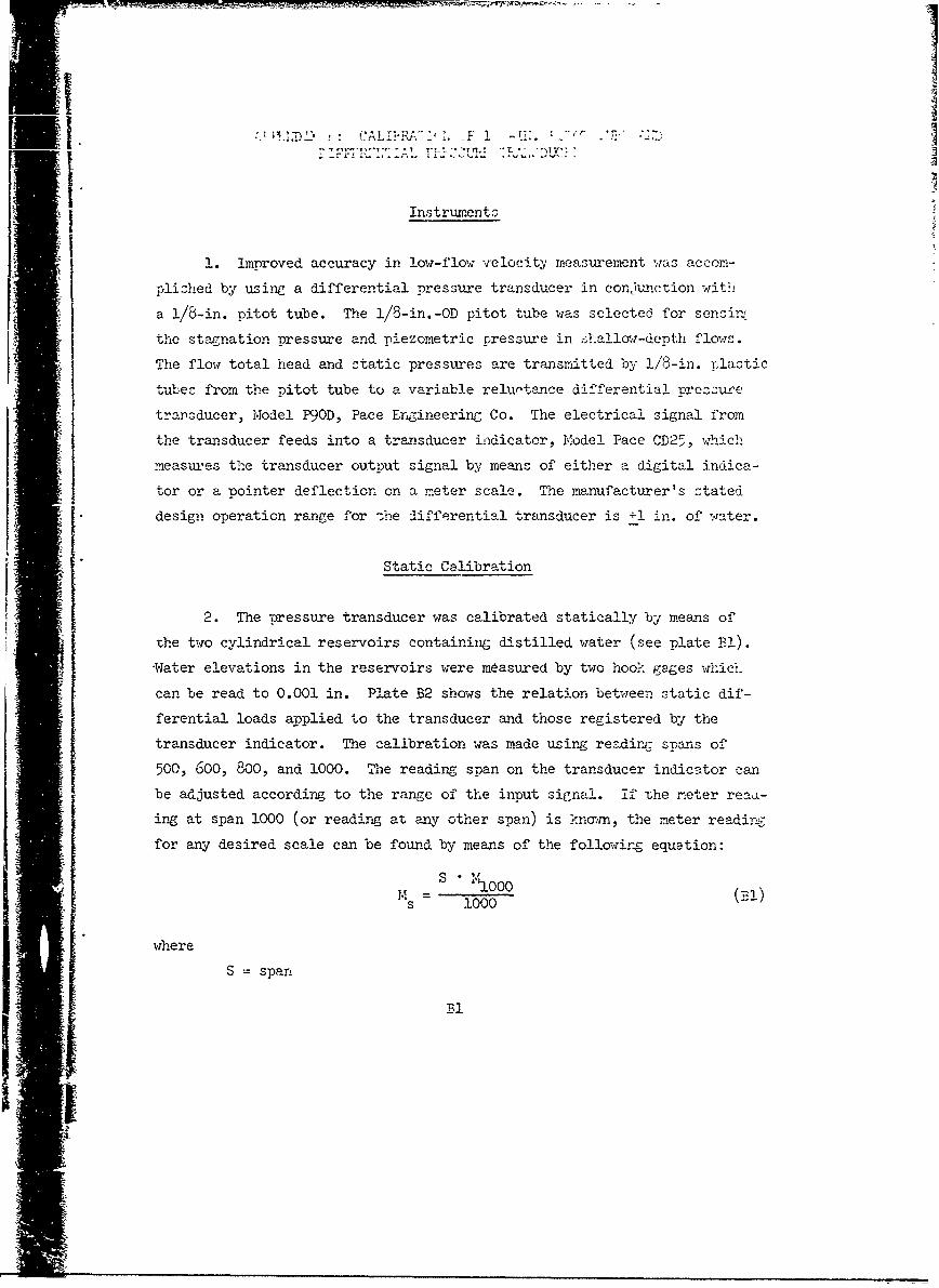
ITTInstrument -

2. improved accuracy in low-flow velocity measurement was accom-

plished by using a differential pressure transducer in conrlunction with

a 1/8-in. pitot tube. The i/8-in.-OD pitot tube was selected for senziit

the stagnation pressure and piezometric pressure in shallow-depth flows.

The flow total head and static pressures are transmitted by !/ 8 -in. plastic

tubes from the pitot tube to a variable reluctance differential prcssure

transducer, Model P9OD, Pace Ergineering Co. The electrical signal from

the transducer feeds into a transducer indicator, Model Pace CD25, which

measures the transducer output signal by means of either a digital indica-

tor or a pointer deflection on a meter scale. The manufacturer's stated

design operation range for -he differential transducer is +1 in. of water.

1-Static Calibration

2. The pressure transducer was calibrated statically by means of

the two cylindrical reservoirs containing distilled water (see plate BI).

-Water elevations in the reservoirs were measured by two hook gages which,

can be read to 0.001 in. Plate B2 shows the relation between static dif-

ferential loads applied to the transducer and those registered by the

transducer indicator. The calibration was made using reading spans of

500, 600, 800, and 1000. The reading span on the transducer indicator can

be adjusted according to the range of the input signal. if the meter reau-

ing at span 1000 (or reading at any other span) is known, the meter reading

for any desired scale can be found by means of the following equation:

S • " , 0 0 0

s 1000

where

S = spar

I .

5 ~' fl~.twer rcadin:v a1t spun 3

meter read-Ing at span 1000

-~rcul: - tatic c-LIibration can be sununiarized by the equation:

Ms o0.1476S Ah (B2)

ml=..

where Anl differential head., in.

Dynamic Calibration

3. The dynamic calibration consisted of an investigation of the

characteristics of the pitot tube and the pressure transducer under dy-

namic loading. The test was performed in a 14-ft-diam circular rotating

tan~k. Plate B3 shows the linearity of the relation between the velocity

head and the meter scale. Comparable static readings for spans 500 and

800 are also shown. The difference between the dynamic and static cali-

bration reflects the pitott tube coefficient which has an average value

of 0.98. Plate Bhl is a direct plot of tank speed and the corresponding

meter readinggs. Plate B5 is a velocity-meter scale plotted on a fuill

logarithmic coordinate. The following relations were derived from the

dynamic calibrations:

i 0.15357 S h h (B3)

or

V = 5.913 4TIjS~ (B4)

where

S. Thelocity head in inches of water

V velocity, fps

Discussions

4. General comments are as follows:

Sof0.9. PateB4 s adirct lotof anksped ad te crreponB2

SI -- ~ ~insensiti-e to the attackr•u-4.,-le i-ithin t~h( rath~e of •, d•with respect to the -main flow direction.-

b. Vibrations. The stein of the pitot tube would vibrate ifi• vortexes were shed periodically from the stem. The vibra-Stions could possib-, produce inaccurate results and zhouldi . not be overlooked, especially under a low Reynolds nmanber•. flow.

c. Reliability, The reliability or the repeatability of thetransducer is reasonably acceptable provided the differen-tial load applied to the transducer is greater than 0.1 in.of water or 0.8 fps in velocity (see plates B3-B5). Over-loading the pressure cell 25 percent does not seem to af-fect the linearity of the transducer output. Further in-formation about the pressure cell can be obtained from theoperational instruction technical manual supplied by thepressure transducer manufacturer.

d. Indicator accuracy. It should be emphasized that the ac-curacy of the indicator as specified by the marnufactureris +1% full scale reading. This factor accounts for thesmaller scattering in the data for the 800 span than for the"500 span in plates B3-B5. Therefore, it is recommended thatthe largest possible span always be used.

e. Signal detection. The developed instrument should not beused to measure the fluctuation components of the turbulenceuntil an improved pressure transmission system replaces theexisting plastic tubing. The latter has a poor frequencyresponse. For measuring the mean velocity of a turbulentflow the digital suppressions control should be used and the

* meter sensitivity switch set on "IN 10, 30, or 100," depend-* ing on the turbulence level. A digital-type voltmeter (inte-

grator) would be desirable for obtaining the mean value ofa random signal.

Operation Comments

5. Operation comments are as follows:

a. Air bubble. The equipment should be set level, with the- I pressure cell located well below the measured flow surface

in order to maintain positive pressure on the pressuretransducer assembly. After the equipment has been properlyconnected, it is necessary to remove any air bubbles from

* A. A. Sooky, "The Flow Through a Meander Flood Plain Geometry," Ph. D.

dissertation, Purdue University, 1964.

* B3

, ., :-'" I ]cr,': rw'o-etiure.- -ire rccomwrenderl (refer to ilate V0L.

(1) CIo.:;u .; 1 and Vrom the nitot tuoe and openvalve 2. Add sufficient distilled water in either ofthe containers and then increase the pressure by anymeans on the container. The air bubbles will be flushedout the by-pass tubing and joints.

(2) Immerse the tip of the pitot tube in the test flow andclose valves 1 and 3 from the bypass line. Increasethe pressure of both water containers separately untilno air bubbles can be observed in the tubings.

(3) Close valves 1 and 3 lines from the pitot tube and closevalve 2. Loosen bleed screws 1 and 2 separately with asmall Allen-head wrench. It will be necessary to movethe cell slightly to gain access to the second bleedscrew. If the water comes out steadily from the airbleed hole, tighten the screws.

b. Zeroing the indicator. Before turning on the power switchof the indicator, the indicating needle should be adjusted,if necessary, to the zero position. The adjusting screw isdirectly beneath the end of the needle. Turn the switch on.Open valve 2 until the water levels in both containers areequal. After selecting a proper "Span," switch the sensi-tivity switch in the "10, SUPPRESSION IN" position. Nowadjust the "Zero Dial" until the indicator needle arrivesat the zero position and lock it by rotating the concentricring clockwise. Close valve 2. If the indicator needle de-flects from zero, check the level of the equipment.

c. Operation (velocity measurement).

(1) Position the pitot tube against the oncoming flow.Close valves 1 and 3 from the water reservoirs andensure that valve 2 is closed.

(2) Switch the sensitivity control to the "100, SUPPRESSIONOUT" position. Adjust the dial until the pointer re-turns to zero. Use "SUPPRESSION OUT, 10" for fine ad-justment. The digits appearing on the dial would bethe meter reading at the particular span.

(3) Use plate B4 or equation B4 to find the velocity infeet per second for the obtained meter reading.

(4) After the velocity measurements have been completed,close valves 1 and 3 to the pitot tube and open valve 2.The velocity data should not be considered reliable un-less the indicator poirter returns to zero. If thepointer fails to return to zero, it may be that some airbubbles have entered the system during the operation.

B4

.1

pernonnel.

()The water should be drairic.l out fromn tthc eju> rnent after

a sequence of' tests is --oomleted.

()Periodic static calibrations are nece:ssary t ensure

that the transducer is operating in a normJ.] function.

B

I.l'i_==

'Iia

*am C

•ii•-B--- I

-t

-1 00 cc I

-UW10 -

ý.::a 'a0w :) z

zz0 )

WU 0

0 ig 0

0

2:

00

PLT J1

- - , 2~fl'"a 'h- ~ ~ ~ 4L~Z~~~ ?.~2o ~ ~r~- 2E

C-1

- 0 00011CV3V 313nd~lVIG0

PLATE B

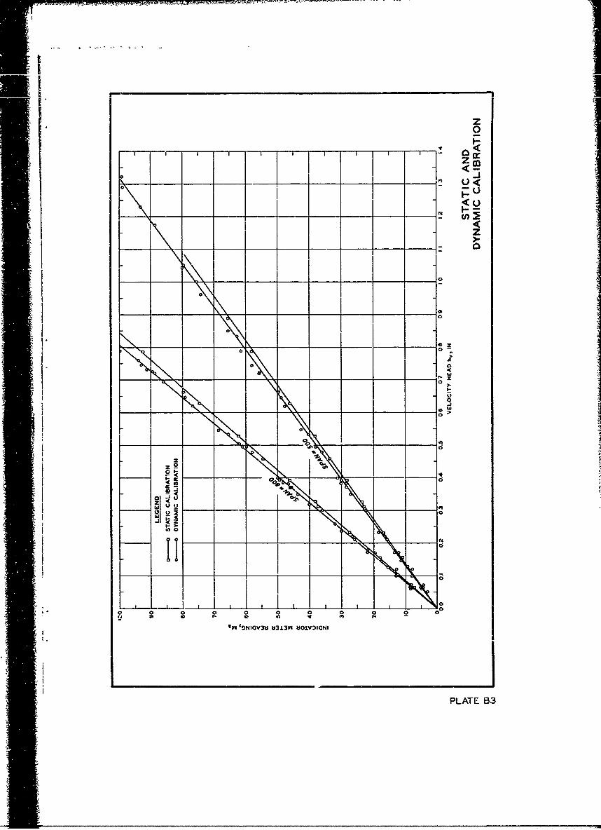
z0

I-.-i-- r -r r T rr r .I I <

-1 >

z 2

2

w0 z

I- 40 -n 0 ) O9Y_ ___GV3 I33 ___ 0 GN

-t - _PLATE _B3

U~~ _wi

r ~n '

00 0 Ir m cu4j

____ ¾ I____ H33V UOI ___ _____ _

PLATE_ B4__I___ __ I___ ___ ___

.10

70---

60-- --- -

50--

lib II

8 I IJ_

i• 0 ' -- 4,- --

i; zzzi izzoi,, z I12 u

03 04 0.5 0.6 0.7 0.8 0.9 1.0 2.0 3.0 4.0

VELOCITY, FPS

DYNAMIC CALIBRATIONLOG-LOG PLOT

PLATE B55