Embed Size (px)
Citation preview
ICES WKDEEP REPORT 2014 ICES ADVISORY COMMITTEE
ICES CM 2014/ACOM:44
Report of the Benchmark Workshop on Deep-sea Stocks (WKDEEP)
3–7 February 2014
Copenhagen, Denmark
International Council for the Exploration of the Sea Conseil International pour l’Exploration de la Mer
H. C. Andersens Boulevard 44–46 DK-1553 Copenhagen V Denmark Telephone (+45) 33 38 67 00 Telefax (+45) 33 93 42 15 www.ices.dk [email protected]
Recommended format for purposes of citation:
ICES. 2015. Report of the Benchmark Workshop on Deep-sea Stocks (WKDEEP), 3–7 February 2014, Copenhagen, Denmark. ICES CM 2014/ACOM:44. 119 pp.
For permission to reproduce material from this publication, please apply to the Gen-eral Secretary.
The document is a report of an Expert Group under the auspices of the International Council for the Exploration of the Sea and does not necessarily represent the views of the Council.
© 2015 International Council for the Exploration of the Sea

ICES WKDEEP REPORT 2014 | i
Contents
Executive summary ................................................................................................................ 3
1 Introduction .................................................................................................................... 4
2 Black scabbardfish ........................................................................................................ 6
2.1 Stock ID and substock structure ......................................................................... 6
2.2 Issue list .................................................................................................................. 6
2.3 Scorecard on data quality .................................................................................... 6 2.4 Multispecies and mixed fisheries issues ............................................................ 6
2.5 Ecosystem drivers ................................................................................................. 7
2.6 Stock assessment ................................................................................................... 7 2.6.1 Catch-quality, misreporting, discards ................................................... 7 2.6.2 Surveys ...................................................................................................... 7 2.6.3 Weights, maturities, growth ................................................................... 8 2.6.4 Assessment model ................................................................................... 8
2.7 Short-term projections .......................................................................................... 9
2.8 Appropriate Reference Points (MSY) ................................................................. 9
2.9 Future research and data requirements ............................................................. 9
2.10 External Reviewers’ comments ......................................................................... 10 2.11 References ............................................................................................................ 11
Appendix 1: Madeira fishery ..................................................................................... 12
Appendix 2: Issue list .................................................................................................. 14
3 Ling in Va ...................................................................................................................... 17
3.1 Stock ID and substock structure: ...................................................................... 17 3.2 Issue list ................................................................................................................ 17
3.3 Scorecard on data quality .................................................................................. 17
3.4 Multispecies and mixed fisheries issues .......................................................... 18 3.5 Ecosystem drivers ............................................................................................... 18
3.6 Stock assessment ................................................................................................. 20 3.6.1 Catch-quality, misreporting, discards ................................................. 20 3.6.2 Surveys .................................................................................................... 20 3.6.3 Weights, maturities, growth ................................................................. 21 3.6.4 Assessment model ................................................................................. 21
3.7 Short-term projections ........................................................................................ 25 3.8 Appropriate reference points (MSY) ................................................................ 25
3.9 Future research and data requirements ........................................................... 27
3.10 External Reviewers Comments ......................................................................... 27
ii | ICES WKDEEP REPORT 2014
4 Blue Ling in Division Vb, and Subareas VI, VII ................................................... 29
4.1 Stock ID and substock structure ....................................................................... 29 4.2 Issue list ................................................................................................................ 29
4.3 Scorecard on data quality .................................................................................. 31
4.4 Multispecies and mixed fisheries issues .......................................................... 31 4.5 Ecosystem drivers ............................................................................................... 31
4.6 Stock Assessment ................................................................................................ 31 4.6.1 Catch-quality, misreporting, discards ................................................. 31 4.6.2 Surveys .................................................................................................... 32 4.6.3 Weights, maturities, growth ................................................................. 32 4.6.4 Assessment model ................................................................................. 32
4.7 Short-term projections ........................................................................................ 34 4.8 Appropriate Reference Points (MSY) ............................................................... 34
4.9 Future research and data requirements ........................................................... 36
4.10 External Reviewers comments .......................................................................... 36
4.11 References ............................................................................................................ 37
5 WKDEEP Conclusions ................................................................................................ 38
5.1 External Reviewers’ comments on blue ling ................................................... 38 5.2 External Reviewers’ comments on ling ........................................................... 38
5.3 External Reviewers’ comments on black scabbardfish .................................. 39
5.4 Conclusions ......................................................................................................... 39
6 Stock annexes ............................................................................................................... 42
6.1 Black scabbardfish stock annex......................................................................... 42
6.2 Ling in Division Va stock annex ....................................................................... 62
6.3 Blue ling in Division Vb, and Subareas VI, VII ............................................... 88
Annex 1: Score Cards ........................................................................................... 106
Annex 2: Participants list .................................................................................... 114
Annex 3: Terms of Reference ............................................................................. 116
ICES WKDEEP REPORT 2014 | 3
Executive summary
The Benchmark Workshop on Deep-sea Stocks 2014 meet in Copenhagen, Denmark at ICES HQ during 3–7 February 2014.
The main goal of the benchmark workshop meeting was to evaluate the appropriate-ness of stock assessment data and methods for the following ICES stocks:
1 ) Blue ling in Division Vb, and Subareas VI, VII; 2 ) Ling in Division Va; 3 ) Black scabbardfish (Aphanopus carbo) in Subareas VI, VII and Divisions Vb
and XIIb; 4 ) Black scabbardfish (Aphanopus carbo) in Subareas VIII and IX; 5 ) Black scabbardfish (Aphanopus carbo) in other areas (Subareas I, II, IV, X,
XIV and Divisions IIIa, Va).
The benchmark focused on compile and evaluate data sources for stock assessment of mentioned stocks, evaluate the assessment models suitable to provide information on the stocks status and to update the relevant stock annexes to provide a comprehen-sive description of the agreed procedure for generating the assessment.
For black scabbard fish it was decided to produce a join assessment for all three stocks as they were considered to be part of a unique single stock that migrates through the Northeast Atlantic and a HCR was agreed. For Ling in Va, new ageing of Icelandic survey data was incorporated into a new Gadget model to derive estimates of FMSY proxies. For blue ling in Division Vb, and Subareas VI, VII, a multiyear catch curve model (MYCC) was used to estimate the total annual mortality, a stock reduc-tion analysis (SRA) was used to predict the biomass dynamics of the stock and a yield-per-recruit model is used to estimate reference points.
4 | ICES WKDEEP REPORT 2014
1 Introduction
The Benchmark Workshop on Deep-sea Stocks was convened in accordance with the ToR (Annex 3) established by ACOM.
The workshop was chaired by External Chair Jim Berkson, USA and ICES Chair Tom Blasdale, UK, and attended by two invited external experts, David Die, USA, and Telmo Morato, Portugal meet in Copenhagen, Denmark at ICES HQ for a 5 day Benchmark meeting 3–7 February 2014. Other participants included members of the ICES stock assessment working groups WGDEEP and members of the ICES secretari-at. A full list of participants is provided in Annex 2.
Previous to the Benchmark workshop a 3 day data compilation workshop (DCWK) was organized at ICES HQ (26–28 November 2013). The DCWK was chaired by ICES Chair Tom Blasdale, (UK) and attended by the invited external expert, David Die (USA) by video conference and the WGDEEP members Pascal Lorance (France), Ivo-ne Figueiredo (Portugal), Gudmundur Thordarson (Iceland) and members of the ICES secretariat.
The data compilation workshop considered the quality of data including discards and estimates of misreporting of landings. During the 3 day workshop the new as-sessment method for the 5 considered stocks were presented, the stocks Score Cards regarding data quality were filled out and a 2014 WGDEEP official Data Call in early 2014 was agreed.
The main goal of the benchmark workshop meeting was to evaluate the appropriate-ness of stock assessment data and methods for the following ICES stocks:
1 ) Blue ling in Division Vb, and Subareas VI, VII; 2 ) Ling in Division Va; 3 ) Black scabbardfish (Aphanopus carbo) in Subareas VI, VII and Divisions Vb
and XIIb; 4 ) Black scabbardfish (Aphanopus carbo) in Subareas VIII and IX; 5 ) Black scabbardfish (Aphanopus carbo) in other areas (Subareas I, II, IV, X,
XIV and Divisions IIIa, Va).
The key aspects of the terms of reference were:
• To compile and evaluate data sources for stock assessment. • Investigate assessment models suitable to provide information on the
stocks status. • To update the relevant stock annexes to provide a comprehensive descrip-
tion of the agreed procedure for generating assessment input data and for conducting the assessment according to the agreed method.
The initial work of the benchmark workshop was devoted to exploratory analyses of the available data with subsequent work focusing on addressing a number of assess-ment issues. It was decided to produce a join assessment for all black scabbardfish stocks as they were considered to be part of a unique single stock that migrates through the Northeast Atlantic.
Sections 2–4 of this report present information for each stock section 7 contains the new ‘stock annexes’ where data and methodology for the assessment the stock status in the incoming years is described.

ICES WKDEEP REPORT 2014 | 5
Evaluation and Recommendations from external experts are included on each stock section and a generic workshop evaluation on section.
6 | ICES WKDEEP REPORT 2014
2 Black scabbardfish
2.1 Stock ID and substock structure
Despite the stock structure of black scabbarddfish it is still uncertain it is admitted the existence of a unique stock along the NE Atlantic. There is a lack of information on some aspects of the biology to fully support this theory of a single stock.
In ICES the one stock hypothesis has been accepted but for advice purposes has con-sidered three management units:
i ) Northern (Divisions Vb and XIIb and Subareas VI and VII); ii ) Southern (Subareas VIII and IX); iii ) Other areas (Divisions IIIa and Va Subareas I, II, IV, X, and XIV).
These management units were established in a way that reflects the main fisheries and their different characteristics to which the species is subjected. The Northern component comprises fish exploited mainly by trawl fisheries while the southern component by a longline fishery. In other areas the species is exploited by both long-liners and trawlers, but the overall landings are much lower than at the other two management units.
2.2 Issue list
See Appendix 2 at the end of this section.
2.3 Scorecard on data quality
Details on data quality are given in Annex 1.
2.4 Multispecies and mixed fisheries issues
In the north of Europe, the species has been mostly captured around the British Isles (ICES Subareas V, VI and VII) and Iceland (ICES Subarea Va) since the early 1990s, following the development of a multispecies deep-water fishery (ICES, 2008, 2010). In the early years of these fisheries, black scabbardfish was mostly discarded as no mar-ket had developed for the species, but it subsequently became one of the main target deep-water species. A large proportion of deep-water trawl catches (upwards of 50%) can consist of unpalatable species and numerous small species, including juveniles of the target species, which are usually discarded (Allain et al., 2003). The main species in the discards of the trawl fishery in by far the Baird's smoothhead (Alepocephalus bairdii) and greater silver smell (Argentina sillus) however, a large number of other non-marketable bentho-pelagic species are discarded. The survival rate of these dis-cards is unknown, but believed to be virtually zero because of fragility of these spe-cies and the effects of pressure changes during retrieval (Gordon, 2001).
In Southern of the fishery takes place at specific fishing grounds off the occidental coast of Portugal, mainly located off Sesimbra (centre of Portugal). The gear is con-sidered highly selective a black scabbardfish represents nearly 90% of the total catch in weight. The main bycatch species are deep-water shark species, mainly Portuguese dogfish (Centrocymnus coelolepis) and leafscale gulper shark (Centrophorus squamosus). Once on board these specimens are dead so the probability of surviving after releas-ing to the sea is null (Bordalo-Machado et al., 2009).
ICES WKDEEP REPORT 2014 | 7
2.5 Ecosystem drivers
There is little information on the main ecosystem driver for the stock along the NE Atlantic. Although the migration pattern of this species have been associated, particu-larly from Madeira spawning grounds to West of the British Island, with feeding on blue whiting (Ribeiro Santos et al., 2013). According to these authors one of the factors that might trigger the migration is associated with the migration pattern of blue whit-ing (M. poutassou), the main prey item of black scabbardfish in the northern area (Ri-beiro Santos et al., 2012).
In the southern area, the species has been associated with steady slopes and sea-mounts (Leite, 1988) that are particularly common in the Mid-Atlantic Ridge (Merrett and Haedrich, 1997) and the Portuguese waters (including Madeira and the Azores). This area, and in terms of its hydrology, is influenced by three water masses: the North Atlantic Central Outflow (NACO), the Mediterranean Outflow (MO) and the North Atlantic Deep Outflow (NADO). The NACO is mainly present down to 500–600 m depth and the NADO predominates below 1400 m (although it is mostly pre-sent under 2000 m); both have a highly significant correlation between salinity and temperature (Pissarra et al., 1983). The influence of the MO is present at depths deep-er than 600 m and down to 2000 m and does not show a correlation between salinity and temperature (Pissarra et al., 1983). This outflow is characterised by relatively sta-ble but high salinities and temperatures (respectively 36.5 and 11.9°C; Pissarra et al., 1983) in relation to the depth at which the species is found. It has several cores alt-hough the two most important lie at 800 m (upper core) and 1200 m (lower core) (Ambar and Howe, 1979). This interval corresponds to the depth at which the black scabbardfish is mainly caught, so the black scabbardfish is commonly associated with MO.
2.6 Stock assessment
2.6.1 Catch-quality, misreporting, discards
The catch data used in model was derived from the two main fisheries in ICES area: the French trawl and Portuguese longline, that operate at the northern area (Subareas Vb and XIIb and Divisions VI and VII) and southern area (ICES Division IXa) respec-tively. The time period considered extends from 1999 to 2012.
In both fisheries the level of discards are considered negligible. Despite the TAC con-strains in previous years particularly in ICES Subareas Vb and XIIb and Divisions VI and VII misreporting seems to have occurred in the early 2000s in EU waters. Im-portant catch data in international waters remain questionable.
The temporal dynamics of the stock within ICES area, which includes migration be-tween the two areas, determines the use of catch data split according to the two fol-lowing period: i) from March to August of an year (referred as the 1st semester); from September to December of an year and January and February of the following year (referred as the 2nd semester).
2.6.2 Surveys
The Scottish survey data could be potentially used to estimate small specimens (total length <70 cm) occurring at BI. This survey is conducted by the Marine Scotland - Science, formerly Fisheries Research Services, along the continental shelf/slope to the northwest of Scotland. The survey was initiated in 1996 with strictly comparable data
8 | ICES WKDEEP REPORT 2014
available between 1998 and 2008. The core area is surveyed between 55o59oN, with trawling undertaken at depths ranging from 300 to 1900 m with most of the hauls being conducted at fixed stations, at depths of around 500 m, 900 m, 1000 m, 1500 m and 1800 m.
2.6.3 Weights, maturities, growth
Details on the species biological aspects are included in stock annex.
2.6.4 Assessment model
The analytical assessment approach developed to evaluate the status of the A. carbo population components living at the northern (BI) and southern area (P), which in-corporates the information on the fisheries, as well as the knowledge available on the biology and the spatial dynamics (including migrations) of the species.
The assessment model is based on two coupled Bayesian state space models of two components (regions) of the population: West of the British Isles (BI) and the Portu-guese mainland (P). In each state–space process divides the population dynamics into two processes that run in parallel: the unobserved process that describes the popula-tion abundance in number, and the observational process that corresponds to the annual catches, also in number.
Coupling of the two models represents the migration from the northern to southern areas. The model contain two length groups (C2 for fish >70 cm <103 cm, and C3 for fish >103 cm), and two semester periods (season 1-from March to August of one year and season 2-September of that year to February of the next year). The main outputs from the model are the estimates of the abundance in number of each length group, along the time, jointly with the respective credible intervals, as well as the posterior distributions of the species´ vital parameters including fishing mortality, for the pop-ulations living in each area.The model estimates the numbers of fish in the latter two length groups and predicts the expected catch from those length groups for the two fisheries for which data were used (French trawlers in the first area and Portuguese longliners in the second area).
The model assumes fish take three semesters to migrate from the BI to P. The only observable parts of the modelled processes relate to the catch of size groups C2 and C3 in the BI and the P. The model also assumes that fishing effort is known (calculat-ed as the ratio of catch to standardized cpue for each fishery) and that the q follow a vague a priori probability distribution and whose parameters are updated throughout the study period. The model estimates migration probabilities, of size groups C2 and C3 from the BI to P and of C3 fish from P to the spawning areas. Recruitment of fish to the C2 length group in the British Isles represents incoming specimens to C2. This recruitment is assumed to occur in the season 2. Emigration of C2 and C3 fish from the BI to P is assumed to occur in season 1 and emigration of C3 from Portugal to the spawning areas only on season 1. Length group transition probabilities represent the probabilities of growing from each length group to the next length group are also estimated for the British Isles and Portugal. Probability of survival from natural caus-es are also estimated by area and assumed to have a priori probability distribution is assumed that is further update along the study period.
The first trial with the model produced a satisfactory fit to the catch observations. A change on the number of semesters during which migration takes place from three to five gave poorer fit and as a consequence a three semester duration was admitted. By

ICES WKDEEP REPORT 2014 | 9
fixing the period it takes fish to migrate from the BI to P to an odd number of semes-ters the model ensures that peaks in predicted abundance occur in both areas during semester 1Posterior distributions of estimated parameters suggest the data are in-formative for the estimation of many parameters given that the posterior distribu-tions differ from the prior distributions.
Given that the model is based on a forward population dynamic model, standard errors of abundance estimates tend to be larger for the early time period than for the most recent period.
2.7 Short-term projections
In future short projections will be performed.
2.8 Appropriate Reference Points (MSY)
The final point of discussion was related to define appropriate estimates of reference points for biomass, fishing mortality and yield.
WGDEEP 2012 (ICES 2012a) used three methods to estimate proxies for MSY refer-ence points (FLAdvice YPR, Extended Beverton and Holt yield simple model (Bhac) and the Gislason method, as recommended in WKLIFE, ICES 2012b). Candidate ref-erence points were within the range that would be considered reasonable for this stock but were not used in advice because, at that time, there was no accepted model that could give reliable estimates of current F and B. Consequently advice in 2012 was given according to method 3.2 in the ICES advice framework for data-limited stocks (ICES 2012b). This method adjusts recent catches in proportion to the recent rate of change in a biomass index and, where absolute estimates of F and B are unavailable, applies a precautionary buffer of 20%. Separate advice was given for the northern and southern stock components based on French and Portuguese commercial cpue series respectively. Trends were estimated from the ratio of the mean index values in the most recent two years to the mean of the previous three years.
In view of the probable linkage between the Portuguese and British Isles fishery components, it is considered essential that the status of the stock as a whole should be considered when giving management advice for either fishery component. However, given the presumed sequential nature of the exploitation pattern, management should also take into consideration trends occurring in the separate areas.
The harvest control rule proposed by WKDEEP 2104 is therefore to adjust catches in both areas according to recent trends in total abundance for the two areas combined as estimated by the state space model (estimated by a regression fitted to the posteri-or median estimates of abundance of the most recent five years). This will be applied in combination with a simple harvest control rule that specifies that catch advice should only increase when the abundance trends for both fishery components are increasing. If either is stable or decreasing, the advised catch for both areas should be adjusted according to the rate of change in the area showing the decrease.
2.9 Future research and data requirements
To get a better on the understanding of species dynamics and how the stock status has evolved along time, several research lines can be identified oriented to:
1 ) Clarify and quantify migratory patterns and stock structure; 2 ) Identify spawning areas throughout the distribution range of the species;
10 | ICES WKDEEP REPORT 2014
3 ) Incorporate fisheries and biological data from the Madeira portion of the stock into the stock model;
4 ) Improve the existent research survey in the northern region to reduce un-certainty on the estimates and develop new surveys along the southern ar-eas for estimating independent abundance and biological indices;
5 ) Improve the understanding of the environmental drivers associated with recruitment and other behaviour patterns such as migration.
Detailed on current and historic data on spatial fleet dynamics catching the species and distribution of fishing effort is in Appendix 1.
2.10 External Reviewers’ comments
Discussion occurred on the issues of whether the assumptions about the model struc-ture (single stock for the British Isles and Portugal, sequential migration, timing of migration) were supported by observations, on what was the appropriate unit of stock for assessment and on the appropriate way to calculate reference points.
The sensitivity of the model to the assumption of the time it takes fish to migrate from the British Isles to the mainland of Portugal was examined during the meeting by changing this parameter from three semesters to five semesters. Model fits to the catch data for five semester migration were generally worse than for a three semester assumption, especially for the most recent period. Estimated trends did not differ much from those estimated for a value of three semesters.
All estimated parameters, including harvest rates, are conditional on the initial popu-lation fed to the model. Interpreting harvest rates as absolute values is therefore prob-lematic because the greater the initial abundance fed to the model the lower the harvest rate (because the catch is the only observation related to abundance).
In the model, recruitment probability is a multiplicative term on the abundance of C2 in the British Isles.
The model estimates such recruitment probability to the British Isles as having a me-dian of 0.27. This corresponds to close to a 30% increase in C2 as result of recruitment every second semester of the year. Figueiredo et al. (2014) report that they use the Scottish survey to define the proportion of C1 in the population and thus calculate the total population in the British Isles from the estimates of C2 obtained in the mod-el. It begs the question of why didn’t the authors use the Scottish survey’s cpue of C1 and C2 as indices of abundance with which to inform the model’s fit. This would require explicitly modelling the abundance of C1 in the British Isles and using the Scottish survey abundance data as part of an observable process that provides infor-mation on the abundance of C1 and C2 in the British Isles. Such a modification would eliminate the awkward assumption that recruitment is a function of C2 abundance. It should only add three new additional parameters to the model, the catchability of the Scottish survey for C2 and C3 and the probability of growing from C1 to C2 but elim-inate one parameter, prBI.
Assumptions about unit of stock
In the past, for assessment purposes, the WGDEEP has considered a north compo-nent that comprises the multispecies trawl fisheries operating in Subareas VI and VII and a south component that includes the longline fishery of mainland Portugal in
ICES WKDEEP REPORT 2014 | 11
Division IXa (ICES, 2011a). ICES has not assessed before the Madeira fishery because it operates outside the ICES area.
Despite the research progress made on some aspects of the species biology and relat-ed fisheries, there is still limited evidence to unequivocally support the currently assumed hypothesis of a single stock in the northeastern Atlantic (Figueiredo et al., 2003; ICES, 2006). This hypothesis, however, is supported by observations that the only region where juveniles smaller than 70 cm are caught is in the northern areas west of the British Isles and spawning has only being confirmed in the southern areas where the Madeira fishery operates.
It was agreed that although it cannot be said that the information unequivocally sup-ports the assumption of a single stock throughout the North Atlantic most of the evi-dence available does supports it. Thus the basic structure of the model seems reasonable because it models the migration process explicitly and does so within a relatively simple model (state space structure rather than age based) that is more likely to be supported by the relative paucity of data on the stock. The model pre-sented at the meeting did not use the data for Madeira because it was not available to the assessment team therefore it did not contribute to the estimation of model param-eters. The stage-based model however does acknowledge the existence of the Madei-ra component of the stock.
It was agreed that it is essential to make an effort to incorporate the available data from the Madeira fishery because this would allow for more accurate estimation of the dynamics of the whole stock, including the component in Portugal that would benefit from the signals coming from the Madeira data in the estimation of emigra-tion rates. Moreover if a new model was to successfully estimate the abundance in the Madeira component of the stock it would provide an estimate of the abundance of the spawning stock that could be related to estimates of recruitment obtained from the British Isles data. Ideally data equivalent to that used for the other two regions should be used (cpue trends and catch to calculate effort, and catch by size group). If only aggregated catch is available the model may still benefit from the additional information contained in the Madeira time-series as it is likely that such catch may help estimates of rates of migration from Portugal to Madeira.
2.11 References Âmbar, I. and Howe, M.R. 1979. Observation of the Mediterranean outflow. I. Mixing in the
Mediterranean outflow. Deep Sea Res., 26A: 535–554.
Bordalo-Machado P., Fernandes A.C., Figueiredo I., Moura O., Reis S., Pestana G., Gordo L.S. 2009. The black scabbardfish (Aphanopus carbo Lowe, 1839) fisheries from the Portuguese mainland and Madeira Island. Sci. Mar. 73, S2, 63–76.
Leite, A.M. 1988. The deep-sea fishery of the black scabbard fish Aphanopus carbo Lowe, 1839 in Madeira Island waters. Proc. World Symp. Fishing Gear and Fishing Vessel Design, Marine In-stitute St John’s, Newfoundland, Canada: 240–243.
Merrett, N. R. and Haedrich, R.L. 1997. Deep-sea demersal fish and fisheries. Chapman and Hall, London.
Pissarra, J.L., Cavaco, M.H. and Leite. 1983. Caracterização oceanográfica na região da Madeira: determinação das massas de água no “núcleo de água mediterrânica”. Bol. Inst. Nac. Invest. Pescas, 10: 65–80.
Ribeiro Santos A., Minto C., Connolly P., Rogan E. 2013. Oocyte dynamics and reproductive strategy of Aphanopus carbo in the NE Atlantic - Implications for fisheries management. Fish. Res. 143, 161–173.
12 | ICES WKDEEP REPORT 2014
Vieira A.R., Farias I., Figueiredo I., Neves A., Morales-Nin B., Sequeira V., Martins M.R., Gordo L.S. 2009. Age and growth of black scabbardfish (Aphanopus carbo Lowe, 1839) in the southern NE Atlantic. Sci. Mar. 73S2, 33–46.
Appendix 1: Madeira fishery
Drifting deep-water longline targeting black scabbardfish (Aphanopus carbo) is the main fishery activity in Madeira Islands. It probably started in the early 1800s when local fisherman were targeting “oil fish”, i.e. deep-water squalid sharks, between 600–800 m depth for its oil to be use in lighting their homes (Noronha, 1925). This fishery was kept almost unaltered for over one century, when in 1982 hemp was replaced by monofilament drifting longline and the number of hooks per line increased (Martins and Ferreira, 1995). This change in fishing gear, along with better equipped boats that helped local fisherman searching for new fishing grounds such as seamounts, signifi-cantly improving their yields (Martins and Ferreira, 1995). The fleet now exploits new areas, especially located SE of Madeira, as far as 150–200 nautical miles from the fish-ing port. The fishery is mostly developed inside the Madeira Exclusive Economic Zone, included in the CECAF 34.1.2 area, all year round. Sporadically fishing sets are made, by the vessels with higher autonomy in the vicinity of the Madeira EEZ.
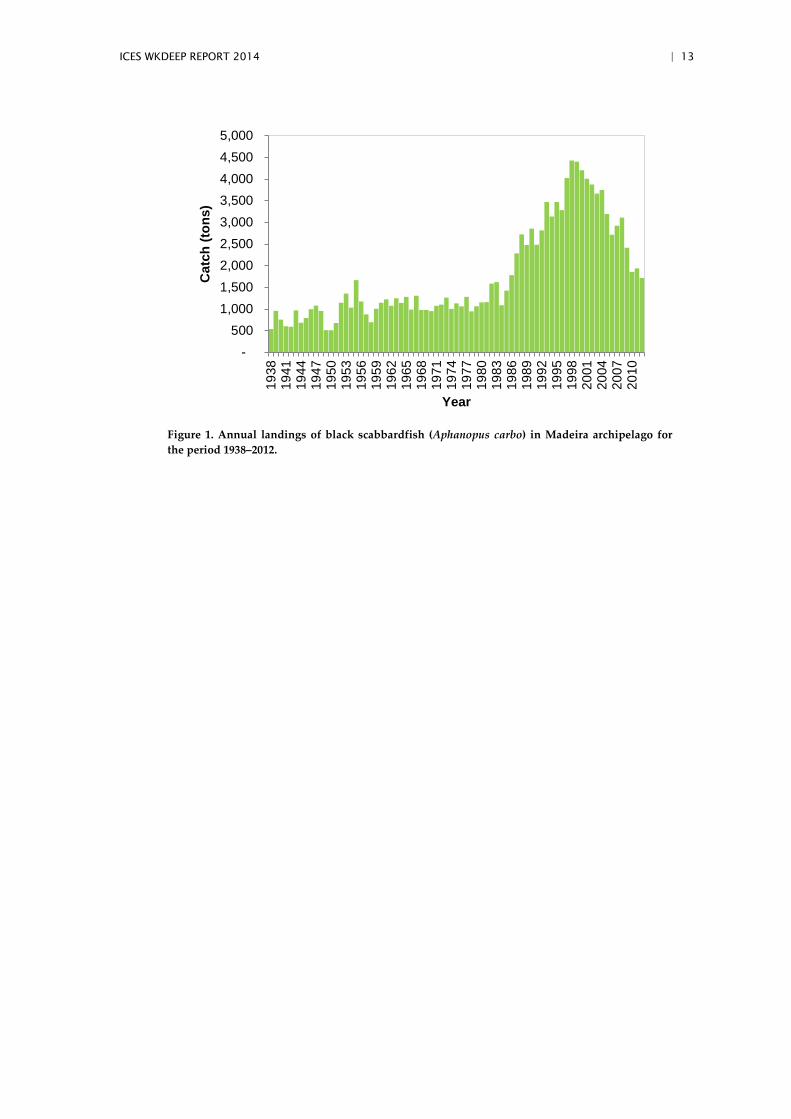
In 1800s, the fleet was composed by about 30 small artisanal vessels (<6 m length) with low engine power. The number of vessels dedicated to this fishery peaked in 1988 with a total of 95 vessels. After that period the fleet suffer a considerable reduc-tion, mainly between 1990 and 1995, when the number of vessels dropped from 84 to 44 (Bordalo-Machado et al., 2009). Between 1998 and 2000, the fleet comprised ca. 40 vessels (on average 13 m LOA, 19 GT and 150 Hp) (Reis et al., 2001). Fleet size contin-ued to decrease to around 15 vessels in the most recent years (2009–2010), with no significant changes in their technical characteristics. Landings of black scabbardfish reached a peak pf 4.2 thousand tonnes in 1998 and have been steadily declining since then to 1.7 thousand tonnes in 2012.
ICES WKDEEP REPORT 2014 | 13
Figure 1. Annual landings of black scabbardfish (Aphanopus carbo) in Madeira archipelago for the period 1938–2012.
- 500
1,000 1,500 2,000 2,500 3,000 3,500 4,000 4,500 5,000
1938
1941
1944
1947
1950
1953
1956
1959
1962
1965
1968
1971
1974
1977
1980
1983
1986
1989
1992
1995
1998
2001
2004
2007
2010
Cat
ch (t
ons)
Year
14 | ICES WKDEEP REPORT 2014
Appendix 2: Issue list
STOCK NE ATLANTIC BLACK SCABBARDFISH
Stock coordinator Name: Ivone Figueiredo E-mail: [email protected]
Stock assessor Name: Ivone Figueiredo E-mail: [email protected]
Data contact Name: E-mail:
ICES WKDEEP REPORT 2014 | 15
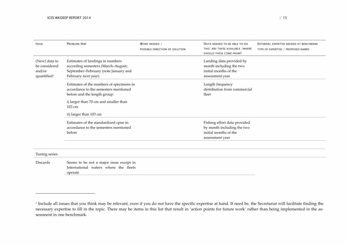
ISSUE PROBLEM/AIM WORK NEEDED / POSSIBLE DIRECTION OF SOLUTION
DATA NEEDED TO BE ABLE TO DO
THIS: ARE THESE AVAILABLE /WHERE
SHOULD THESE COME FROM?
EXTERNAL EXPERTISE NEEDED AT BENCHMARK TYPE OF EXPERTISE / PROPOSED NAMES
(New) data to be considered and/or quantified1
Estimates of landings in numbers according semesters (March–August; September–February (note January and February next year)
Landing data provided by month including the two initial months of the assessment year
Estimates of the numbers of specimens in accordance to the semesters mentioned before and the length group:
i) larger than 70 cm and smaller than 103 cm
ii) larger than 103 cm
Length frequency distribution from commercial fleet
Estimates of the standardized cpue in accordance to the semesters mentioned before
Fishing effort data provided by month including the two initial months of the assessment year
Tuning series
Discards Seems to be not a major issue except in International waters where the fleets operate
1 Include all issues that you think may be relevant, even if you do not have the specific expertise at hand. If need be, the Secretariat will facilitate finding the necessary expertise to fill in the topic. There may be items in this list that result in ‘action points for future work’ rather than being implemented in the as-sessment in one benchmark.
16 | ICES WKDEEP REPORT 2014
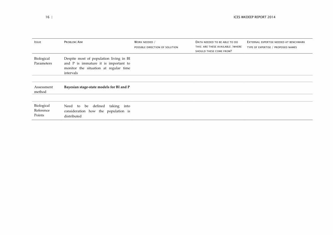
ISSUE PROBLEM/AIM WORK NEEDED / POSSIBLE DIRECTION OF SOLUTION
DATA NEEDED TO BE ABLE TO DO
THIS: ARE THESE AVAILABLE /WHERE
SHOULD THESE COME FROM?
EXTERNAL EXPERTISE NEEDED AT BENCHMARK TYPE OF EXPERTISE / PROPOSED NAMES
Biological Parameters
Despite most of population living in BI and P is immature it is important to monitor the situation at regular time intervals
Assessment method
Bayesian stage-state models for BI and P
Biological Reference Points
Need to be defined taking into consideration how the population is distributed
ICES WKDEEP REPORT 2014 | 17
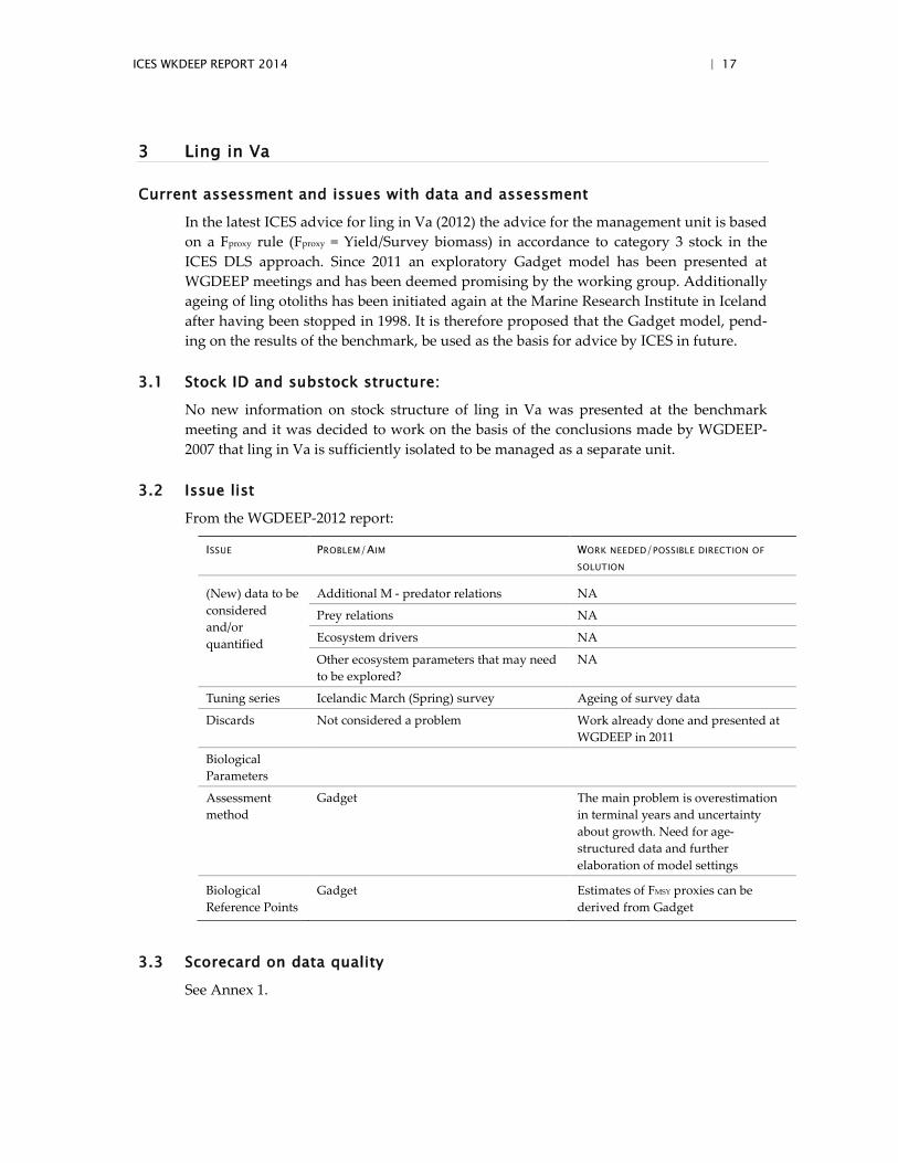
3 Ling in Va
Current assessment and issues with data and assessment
In the latest ICES advice for ling in Va (2012) the advice for the management unit is based on a Fproxy rule (Fproxy = Yield/Survey biomass) in accordance to category 3 stock in the ICES DLS approach. Since 2011 an exploratory Gadget model has been presented at WGDEEP meetings and has been deemed promising by the working group. Additionally ageing of ling otoliths has been initiated again at the Marine Research Institute in Iceland after having been stopped in 1998. It is therefore proposed that the Gadget model, pend-ing on the results of the benchmark, be used as the basis for advice by ICES in future.
3.1 Stock ID and substock structure:
No new information on stock structure of ling in Va was presented at the benchmark meeting and it was decided to work on the basis of the conclusions made by WGDEEP-2007 that ling in Va is sufficiently isolated to be managed as a separate unit.
3.2 Issue list
From the WGDEEP-2012 report:
ISSUE PROBLEM/AIM WORK NEEDED/POSSIBLE DIRECTION OF
SOLUTION
(New) data to be considered and/or quantified
Additional M - predator relations NA
Prey relations NA
Ecosystem drivers NA
Other ecosystem parameters that may need to be explored?
NA
Tuning series Icelandic March (Spring) survey Ageing of survey data
Discards Not considered a problem Work already done and presented at WGDEEP in 2011
Biological Parameters
Assessment method
Gadget The main problem is overestimation in terminal years and uncertainty about growth. Need for age-structured data and further elaboration of model settings
Biological Reference Points
Gadget Estimates of FMSY proxies can be derived from Gadget
3.3 Scorecard on data quality
See Annex 1.
18 | ICES WKDEEP REPORT 2014
3.4 Multispecies and mixed fisheries issues
Ling is caught in mixed fisheries in Va with cod, haddock and other demersal stocks in trawls, longlines, gillnets and other gears. Ling is seldom caught in direct fisheries in Va. The Icelandic management system has various measures to deal with these kind of tech-nical interactions such as transfer of quota between boats, years and species, See the stock annex for details.
Multispecies effects on ling stock dynamics are not known.
3.5 Ecosystem drivers
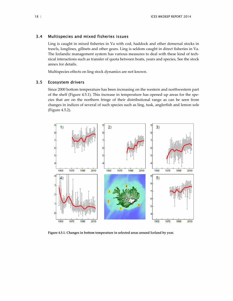
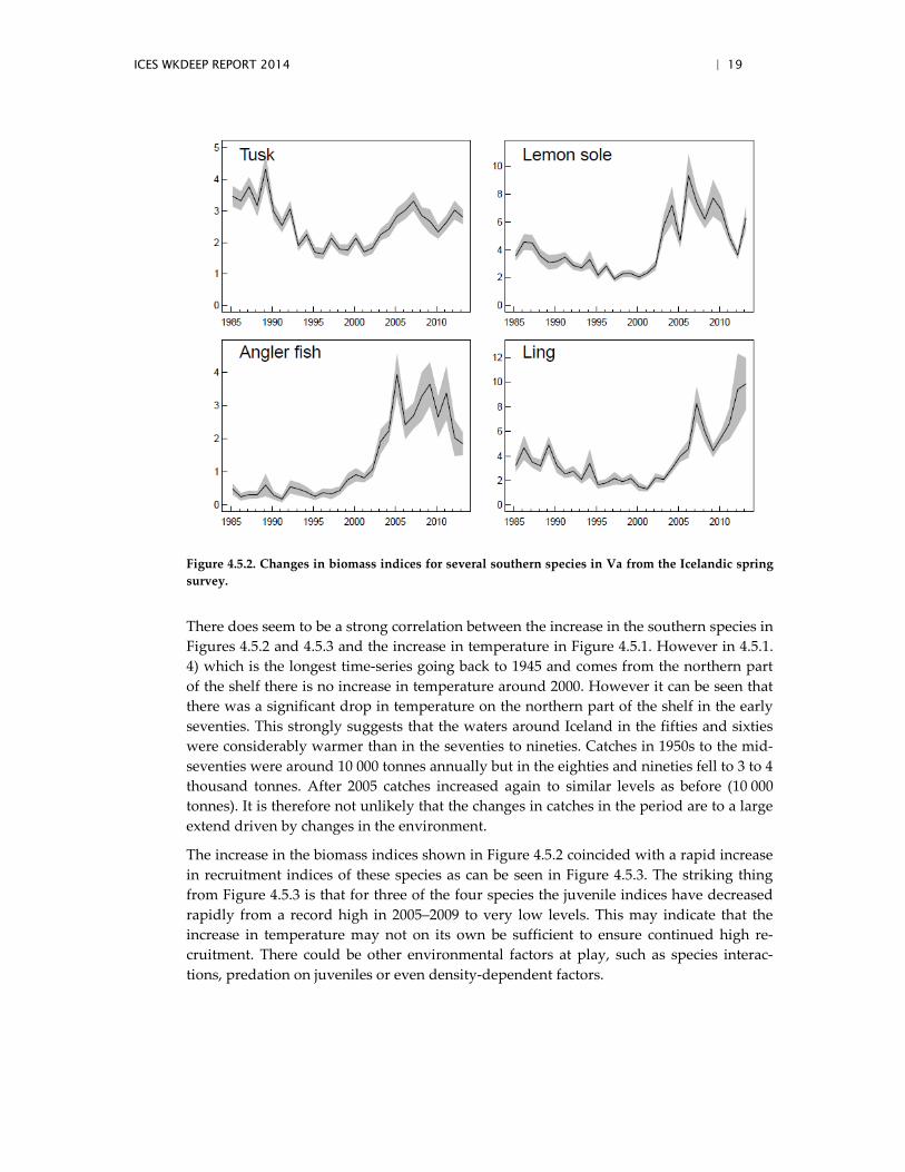
Since 2000 bottom temperature has been increasing on the western and northwestern part of the shelf (Figure 4.5.1). This increase in temperature has opened up areas for the spe-cies that are on the northern fringe of their distributional range as can be seen from changes in indices of several of such species such as ling, tusk, anglerfish and lemon sole (Figure 4.5.2).
Figure 4.5.1. Changes in bottom temperature in selected areas around Iceland by year.
ICES WKDEEP REPORT 2014 | 19
Figure 4.5.2. Changes in biomass indices for several southern species in Va from the Icelandic spring survey.
There does seem to be a strong correlation between the increase in the southern species in Figures 4.5.2 and 4.5.3 and the increase in temperature in Figure 4.5.1. However in 4.5.1. 4) which is the longest time-series going back to 1945 and comes from the northern part of the shelf there is no increase in temperature around 2000. However it can be seen that there was a significant drop in temperature on the northern part of the shelf in the early seventies. This strongly suggests that the waters around Iceland in the fifties and sixties were considerably warmer than in the seventies to nineties. Catches in 1950s to the mid-seventies were around 10 000 tonnes annually but in the eighties and nineties fell to 3 to 4 thousand tonnes. After 2005 catches increased again to similar levels as before (10 000 tonnes). It is therefore not unlikely that the changes in catches in the period are to a large extend driven by changes in the environment.
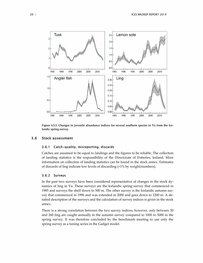
The increase in the biomass indices shown in Figure 4.5.2 coincided with a rapid increase in recruitment indices of these species as can be seen in Figure 4.5.3. The striking thing from Figure 4.5.3 is that for three of the four species the juvenile indices have decreased rapidly from a record high in 2005–2009 to very low levels. This may indicate that the increase in temperature may not on its own be sufficient to ensure continued high re-cruitment. There could be other environmental factors at play, such as species interac-tions, predation on juveniles or even density-dependent factors.
20 | ICES WKDEEP REPORT 2014
Figure 4.5.3. Changes in juvenile abundance indices for several southern species in Va from the Ice-landic spring survey.
3.6 Stock assessment
3.6.1 Catch-quality, misreporting, discards
Catches are assumed to be equal to landings and the figures to be reliable. The collection of landing statistics is the responsibility of the Directorate of Fisheries, Iceland. More information on collection of landing statistics can be found in the stock annex. Estimates of discards of ling indicate low levels of discarding (<1% by weight/numbers).
3.6.2 Surveys
In the past two surveys have been considered representative of changes in the stock dy-namics of ling in Va. These surveys are the Icelandic spring survey that commenced in 1985 and surveys the shelf down to 500 m. The other survey is the Icelandic autumn sur-vey that commenced in 1996 and was extended in 2000 and goes down to 1200 m. A de-tailed description of the surveys and the calculation of survey indices is given in the stock annex.
There is a strong correlation between the two survey indices; however, only between 30 and 260 ling are caught annually in the autumn survey compared to 1000 to 5000 in the spring survey. It was therefore concluded by the benchmark meeting to use only the spring survey as a tuning series in the Gadget model.
ICES WKDEEP REPORT 2014 | 21
3.6.3 Weights, maturities, growth
Mean weight-at-age in the survey and in the commercial catches in the assessment (Gadget) is estimated internally in the model using the available otolith data and a length–weight relationship estimated from data collected in the spring survey. Overview of the available aged otoliths is given in a working document on the ling assessment pre-sented at the benchmark (WD-01). Information on growth is similarly obtained from the available otolith data and is estimated in the model.
3.6.4 Assessment model
At the meeting a Gadget model for ling was proposed as an assessment model. Gadget is shorthand for the "Globally applicable Area Disaggregated General Ecosystem Toolbox", which is a statistical model of marine ecosystems. Gadget (previously known as BOR-MICON and Fleksibest). Gadget is an age–length structured forward-simulation model, coupled with an extensive set of data comparison and optimisation routines. Processes are generally modelled as dependent on length, but age is tracked in the models, and data can be compared on either a length and/or age scale. The model is designed as a multi-area, multi-area, multifleet model, capable of including predation and mixed fish-eries issues; however it can also be used on a single species basis. Detailed description of the Gadget model and references to published papers can be found in the stock annex for ling in Va. Gadget is distinguished from many stock assessment models used within ICES (such as XSA) in that Gadget is a forward simulation model, and is structured be both age and length. It therefore requires direct modelling of growth within the model.
Below a very brief description of the input data, model settings, parameters estimated and the procedure used for assigning weights to the likelihood components is given. A more detailed description can be found in WD-01 and in the stock annex.
Input data
The input data comes from the three main commercial fleets catching ling in Va (longline, trawl and gillnet) and the Icelandic spring survey.
• Length disaggregated survey indices (10 cm increments, except the smallest 20–50 cm and the largest 90–180 cm) from the Icelandic groundfish survey in March 1985–onwards.
• Length distribution from the Icelandic commercial catch since 1982. The sam-pling effort was though relatively limited until the 1990s.
• Landings data divided into four month periods per year (quarters). • Age–length data from the survey and from the commercial fleets.
To estimate the uncertainty in the model parameters and derived quantities a specialized bootstrap for disparate datasets is used. The approach is based on spatial subdivisions that can be considered to be i.i.d. Refer to Elvarsson et al. (2014) for further details.
Model settings
The population is defined by 1 cm length groups, from 20–180 cm and the year is divided into four quarters. The age range is 2 to 20 years, with the oldest age treated as a plus group. Recruitment takes place in the first quarter and is set at age 2. The length-at-
22 | ICES WKDEEP REPORT 2014
recruitment is estimated and growth is assumed to follow the von Bertalanffy growth function estimated by the model. The weight–length relationship is obtained from data collected in the spring survey. Natural mortality (M) is assumed to be 0.15.
The commercial landings are modelled as three fleets, longline, trawl and gillnet, starting in 1982 with a selection patterns described by a logistic function and the total catch in tonnes specified for each quarter. The survey (1985 onwards), on the other hand is mod-elled as one fleet with constant effort and a nonparametric selection pattern that is esti-mated for each length group (one 10 cm length group).
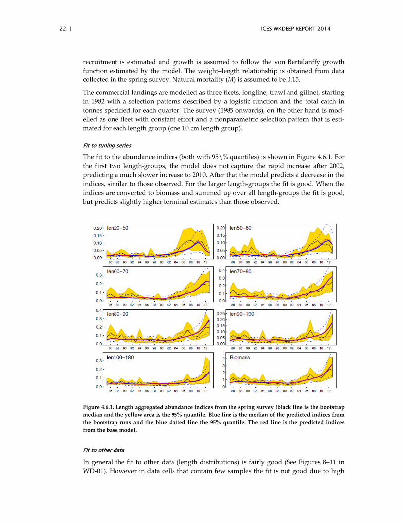
Fit to tuning series
The fit to the abundance indices (both with 95\% quantiles) is shown in Figure 4.6.1. For the first two length-groups, the model does not capture the rapid increase after 2002, predicting a much slower increase to 2010. After that the model predicts a decrease in the indices, similar to those observed. For the larger length-groups the fit is good. When the indices are converted to biomass and summed up over all length-groups the fit is good, but predicts slightly higher terminal estimates than those observed.
Figure 4.6.1. Length aggregated abundance indices from the spring survey (black line is the bootstrap median and the yellow area is the 95% quantile. Blue line is the median of the predicted indices from the bootstrap runs and the blue dotted line the 95% quantile. The red line is the predicted indices from the base model.
Fit to other data
In general the fit to other data (length distributions) is fairly good (See Figures 8–11 in WD-01). However in data cells that contain few samples the fit is not good due to high
ICES WKDEEP REPORT 2014 | 23
variance in the data cells, this particularly is the case at the beginning of the time-series (before 1998).
Estimates
Growth as estimated in the model is similar to what can be observed in the limited age-structured data. There are though discrepancies between the estimated mean length-at-age and the observed for the older age-groups. According to the estimated catch-at-age distributions, most of the ling is between the age of 6 and 12 and in the stock there is no sign of a large plus group. L50 for the longline-, trawl- and survey-fleet are at a similar range, around 70 cm but the slope is markedly different, especially in the survey where it has the lowest slope. The gillnet fleet L50 is close to 100 but due to few data from gillnets the model has difficulty estimating the selection parameters.
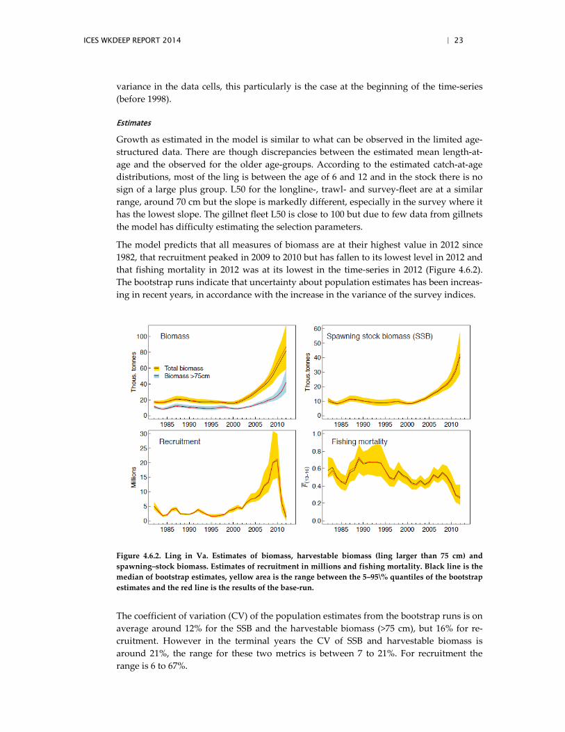
The model predicts that all measures of biomass are at their highest value in 2012 since 1982, that recruitment peaked in 2009 to 2010 but has fallen to its lowest level in 2012 and that fishing mortality in 2012 was at its lowest in the time-series in 2012 (Figure 4.6.2). The bootstrap runs indicate that uncertainty about population estimates has been increas-ing in recent years, in accordance with the increase in the variance of the survey indices.
Figure 4.6.2. Ling in Va. Estimates of biomass, harvestable biomass (ling larger than 75 cm) and spawning–stock biomass. Estimates of recruitment in millions and fishing mortality. Black line is the median of bootstrap estimates, yellow area is the range between the 5–95\% quantiles of the bootstrap estimates and the red line is the results of the base-run.
The coefficient of variation (CV) of the population estimates from the bootstrap runs is on average around 12% for the SSB and the harvestable biomass (>75 cm), but 16% for re-cruitment. However in the terminal years the CV of SSB and harvestable biomass is around 21%, the range for these two metrics is between 7 to 21%. For recruitment the range is 6 to 67%.
24 | ICES WKDEEP REPORT 2014
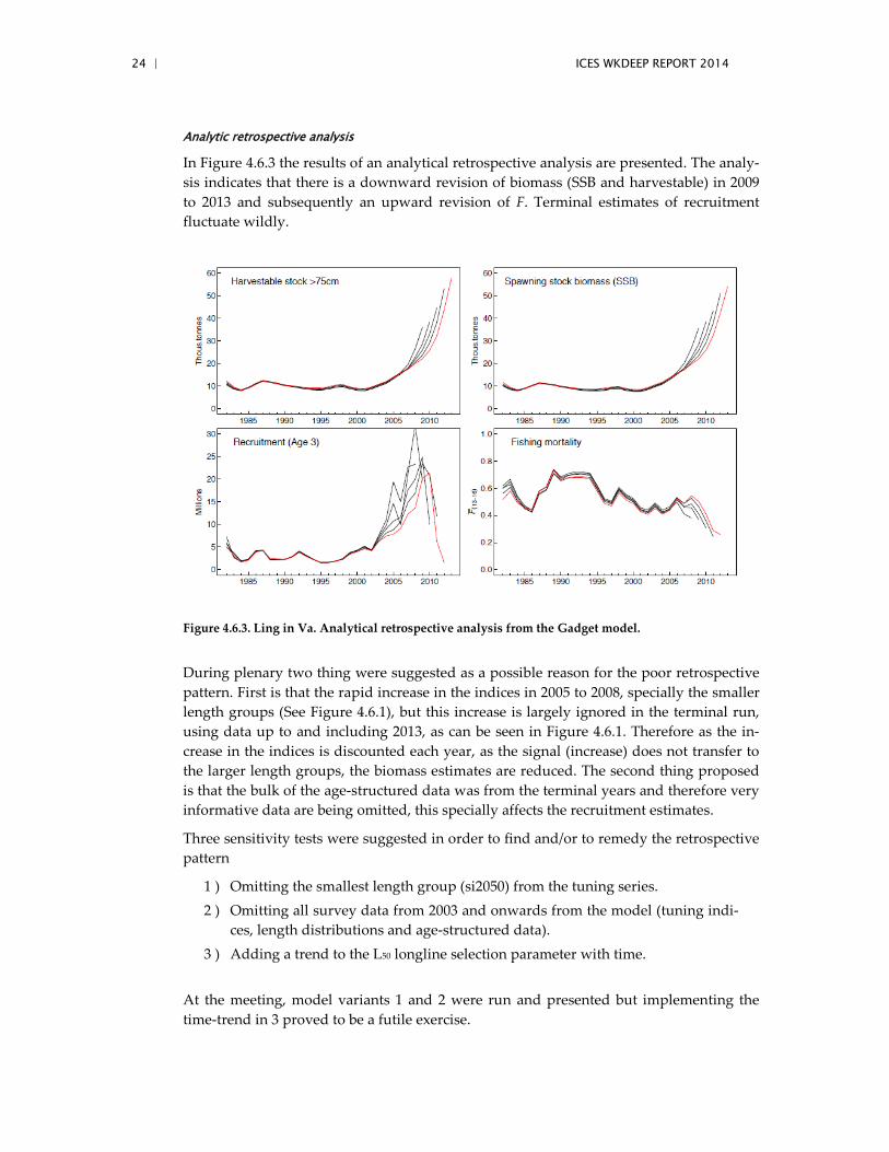
Analytic retrospective analysis
In Figure 4.6.3 the results of an analytical retrospective analysis are presented. The analy-sis indicates that there is a downward revision of biomass (SSB and harvestable) in 2009 to 2013 and subsequently an upward revision of F. Terminal estimates of recruitment fluctuate wildly.
Figure 4.6.3. Ling in Va. Analytical retrospective analysis from the Gadget model.
During plenary two thing were suggested as a possible reason for the poor retrospective pattern. First is that the rapid increase in the indices in 2005 to 2008, specially the smaller length groups (See Figure 4.6.1), but this increase is largely ignored in the terminal run, using data up to and including 2013, as can be seen in Figure 4.6.1. Therefore as the in-crease in the indices is discounted each year, as the signal (increase) does not transfer to the larger length groups, the biomass estimates are reduced. The second thing proposed is that the bulk of the age-structured data was from the terminal years and therefore very informative data are being omitted, this specially affects the recruitment estimates.
Three sensitivity tests were suggested in order to find and/or to remedy the retrospective pattern
1 ) Omitting the smallest length group (si2050) from the tuning series. 2 ) Omitting all survey data from 2003 and onwards from the model (tuning indi-
ces, length distributions and age-structured data). 3 ) Adding a trend to the L50 longline selection parameter with time.
At the meeting, model variants 1 and 2 were run and presented but implementing the time-trend in 3 proved to be a futile exercise.
ICES WKDEEP REPORT 2014 | 25
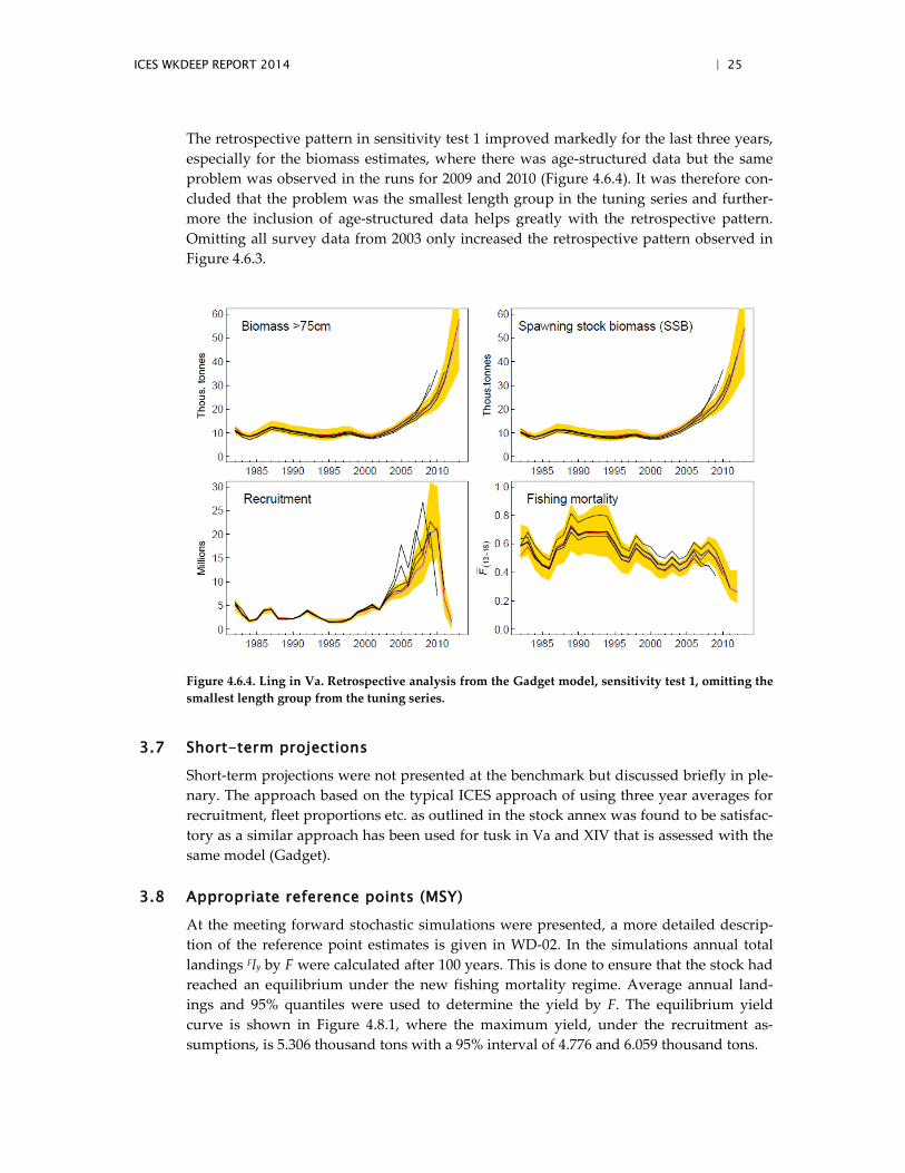
The retrospective pattern in sensitivity test 1 improved markedly for the last three years, especially for the biomass estimates, where there was age-structured data but the same problem was observed in the runs for 2009 and 2010 (Figure 4.6.4). It was therefore con-cluded that the problem was the smallest length group in the tuning series and further-more the inclusion of age-structured data helps greatly with the retrospective pattern. Omitting all survey data from 2003 only increased the retrospective pattern observed in Figure 4.6.3.
Figure 4.6.4. Ling in Va. Retrospective analysis from the Gadget model, sensitivity test 1, omitting the smallest length group from the tuning series.
3.7 Short-term projections
Short-term projections were not presented at the benchmark but discussed briefly in ple-nary. The approach based on the typical ICES approach of using three year averages for recruitment, fleet proportions etc. as outlined in the stock annex was found to be satisfac-tory as a similar approach has been used for tusk in Va and XIV that is assessed with the same model (Gadget).
3.8 Appropriate reference points (MSY)
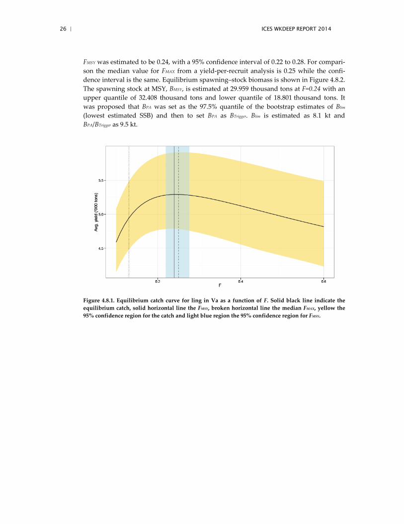
At the meeting forward stochastic simulations were presented, a more detailed descrip-tion of the reference point estimates is given in WD-02. In the simulations annual total landings Fly by F were calculated after 100 years. This is done to ensure that the stock had reached an equilibrium under the new fishing mortality regime. Average annual land-ings and 95% quantiles were used to determine the yield by F. The equilibrium yield curve is shown in Figure 4.8.1, where the maximum yield, under the recruitment as-sumptions, is 5.306 thousand tons with a 95% interval of 4.776 and 6.059 thousand tons.
26 | ICES WKDEEP REPORT 2014
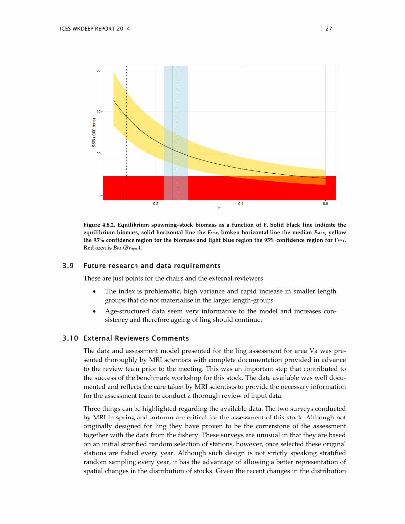
FMSY was estimated to be 0.24, with a 95% confidence interval of 0.22 to 0.28. For compari-son the median value for FMAX from a yield-per-recruit analysis is 0.25 while the confi-dence interval is the same. Equilibrium spawning–stock biomass is shown in Figure 4.8.2. The spawning stock at MSY, BMSY, is estimated at 29.959 thousand tons at F=0.24 with an upper quantile of 32.408 thousand tons and lower quantile of 18.801 thousand tons. It was proposed that BPA was set as the 97.5% quantile of the bootstrap estimates of Blim (lowest estimated SSB) and then to set BPA as BTrigger. Blim is estimated as 8.1 kt and BPA/BTrigger as 9.5 kt.
Figure 4.8.1. Equilibrium catch curve for ling in Va as a function of F. Solid black line indicate the equilibrium catch, solid horizontal line the FMSY, broken horizontal line the median FMAX, yellow the 95% confidence region for the catch and light blue region the 95% confidence region for FMSY.
ICES WKDEEP REPORT 2014 | 27
Figure 4.8.2. Equilibrium spawning–stock biomass as a function of F. Solid black line indicate the equilibrium biomass, solid horizontal line the FMSY, broken horizontal line the median FMAX, yellow the 95% confidence region for the biomass and light blue region the 95% confidence region for FMSY. Red area is BPA (BTrigger).
3.9 Future research and data requirements
These are just points for the chairs and the external reviewers
• The index is problematic, high variance and rapid increase in smaller length groups that do not materialise in the larger length-groups.
• Age-structured data seem very informative to the model and increases con-sistency and therefore ageing of ling should continue.
3.10 External Reviewers Comments
The data and assessment model presented for the ling assessment for area Va was pre-sented thoroughly by MRI scientists with complete documentation provided in advance to the review team prior to the meeting. This was an important step that contributed to the success of the benchmark workshop for this stock. The data available was well docu-mented and reflects the care taken by MRI scientists to provide the necessary information for the assessment team to conduct a thorough review of input data.
Three things can be highlighted regarding the available data. The two surveys conducted by MRI in spring and autumn are critical for the assessment of this stock. Although not originally designed for ling they have proven to be the cornerstone of the assessment together with the data from the fishery. These surveys are unusual in that they are based on an initial stratified random selection of stations, however, once selected these original stations are fished every year. Although such design is not strictly speaking stratified random sampling every year, it has the advantage of allowing a better representation of spatial changes in the distribution of stocks. Given the recent changes in the distribution
28 | ICES WKDEEP REPORT 2014
of ling observed in the last decade, it seems that the decision to use stations as fixed sta-tions was, at least for ling, a wise decision. The large number of stations sampled sup-ports also the argument that these surveys produce reliable indices of abundances for ling, at least for the larger length classes (during the meeting it was concluded that indi-ces for the smallest size groups may have created the retrospective patterns in fishing mortality observed in the results).
The recent restart of the program of collection of ling age samples has clearly benefited and enriched the information available for assessment. It is essential that this program be maintained so as to reduce the uncertainty in the estimations of stock status. It is possible that a focus on ageing the smallest fish in the survey catch may help reduce the uncer-tainty associated with estimates of recruitment. Estimates based on catch rates of the smallest size ranges prove to be unreliable during the recent period of high recruitment. This could be the result of many things but one possible reason could be that small fish have variable growth rates and therefore that in different years the same length groups may represent different age groups. Understanding whether ling does show variable growth at young ages may therefore help reduce uncertainty in estimates of recruitment.
The assessment model used, GADGET, is very flexible in its ability to integrate different types of data and able to cope also with various levels of data availability. It seems well suited for the assessment of ling. Its power to explicitly model length distributions and to do so by length transition matrices allows it to make changes in the length distribution to persist between subsequent time periods, something that other models that redistribute lengths between subsequent time periods cannot do. Whether such ability is critical for the assessment of ling is unclear. If it was proven that variable growth rates are an im-portant characteristic of the dynamics of this stock or that selectivity does alter the length distribution of cohorts by preferentially removing the fast growing fish, then GADGET would be a superior model to use compared with others like SS. On the other hand GADGET has very long running times compared to SS. The complexity of the GADGET model and its required run time limited our ability to conduct and review a thorough sensitivity analysis of the model to different assumptions or input data during the benchmark meeting. If this model is to be used in future benchmarks for this stock, the review panel suggests that a more thorough sensitivity analysis be conducted prior to the meeting enabling its review during the meeting.
ICES WKDEEP REPORT 2014 | 29
4 Blue Ling in Division Vb, and Subareas VI, VII
4.1 Stock ID and substock structure
No new information on stock structure of blue ling in VB, VI and VII was presented at the benchmark meeting (see stock annex for current stock definition).
The only area where some juveniles may occur are Faroese waters. The number of juve-niles observed in Faroese waters does not, by far, seem sufficient to sustain the recruit-ment of adult blue ling in Vb, VI and VII. In the neighbouring ICES Division XIIb, from where landings have been less than 100 tonnes to a few hundred tonnes in recent years but have been higher in the past, the situation is the same: there are no juveniles and only adult fish are known to occur. As the western Hatton Bank in XIIb is the continuation to the west of the Bank located in VIb, blue ling in ICES Division XIIb may belong to the same biological population as blue ling in Vb, VI and VII.
The group discussed the hypothesis that blue ling in the assessment area may recruit from Iceland, the only region were significant nurseries are known.
Although the stock identity may deserve further work, this does not precludes blue ling for ICES subareas VI and VII and Division Vb (and possibly XIIb) to be assessed as a stock unit. In this unit fish recruit to the fishery mostly at an age of 8 and 9 and there is no indication that adult blue ling further emigrates from the area. Therefore the stock assessment based on catch curve of adult fish, estimation of recruitment at age 8-9 and modelling of the dynamics of adult fish is appropriate. The assessment aims at estimating the fishing mortality, stock number and biomass of a stock of mature adult fish.
4.2 Issue list
Table 3.1. List of issues and work to do, prior to and at the benchmark, modified from the WGDEEP (2012).
Issue Problem/Aim
Work needed/possible direction of solution
Data needed to be able to do this: are these available/where should these come from?
(New) data to be considered and/or quantified
Additional M - predator relations
Review of M estimates
Archive data on age and length distribution. Output of MYCC
Prey relations Not known Feeding is known
Ecosystem drivers Not known NA
Other ecosystem parameters that may need to be explored?
Impact of fishing on the ecosystem
The impact of fishing on deep-water is addressed by WGDEC
30 | ICES WKDEEP REPORT 2014
Issue Problem/Aim
Work needed/possible direction of solution
Data needed to be able to do this: are these available/where should these come from?
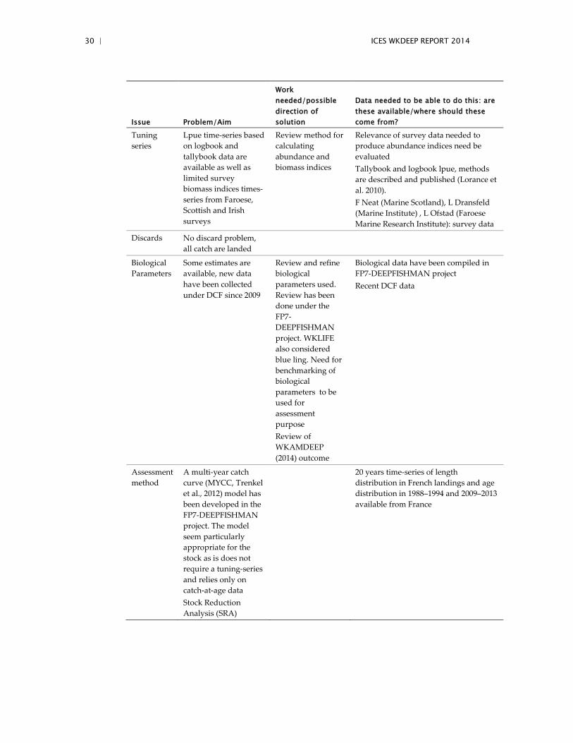
Tuning series
Lpue time-series based on logbook and tallybook data are available as well as limited survey biomass indices times-series from Faroese, Scottish and Irish surveys
Review method for calculating abundance and biomass indices
Relevance of survey data needed to produce abundance indices need be evaluated Tallybook and logbook lpue, methods are described and published (Lorance et al. 2010). F Neat (Marine Scotland), L Dransfeld (Marine Institute) , L Ofstad (Faroese Marine Research Institute): survey data
Discards No discard problem, all catch are landed
Biological Parameters
Some estimates are available, new data have been collected under DCF since 2009
Review and refine biological parameters used. Review has been done under the FP7-DEEPFISHMAN project. WKLIFE also considered blue ling. Need for benchmarking of biological parameters to be used for assessment purpose Review of WKAMDEEP (2014) outcome
Biological data have been compiled in FP7-DEEPFISHMAN project Recent DCF data
Assessment method
A multi-year catch curve (MYCC, Trenkel et al., 2012) model has been developed in the FP7-DEEPFISHMAN project. The model seem particularly appropriate for the stock as is does not require a tuning-series and relies only on catch-at-age data Stock Reduction Analysis (SRA)
20 years time-series of length distribution in French landings and age distribution in 1988–1994 and 2009–2013 available from France
ICES WKDEEP REPORT 2014 | 31
Issue Problem/Aim
Work needed/possible direction of solution
Data needed to be able to do this: are these available/where should these come from?
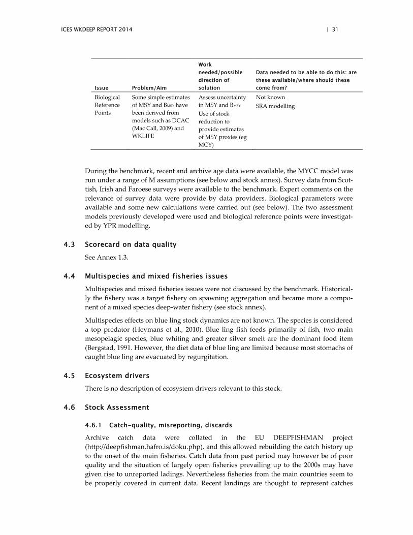
Biological Reference Points
Some simple estimates of MSY and BMSY have been derived from models such as DCAC (Mac Call, 2009) and WKLIFE
Assess uncertainty in MSY and BMSY Use of stock reduction to provide estimates of MSY proxies (eg MCY)
Not known SRA modelling
During the benchmark, recent and archive age data were available, the MYCC model was run under a range of M assumptions (see below and stock annex). Survey data from Scot-tish, Irish and Faroese surveys were available to the benchmark. Expert comments on the relevance of survey data were provide by data providers. Biological parameters were available and some new calculations were carried out (see below). The two assessment models previously developed were used and biological reference points were investigat-ed by YPR modelling.
4.3 Scorecard on data quality
See Annex 1.3.
4.4 Multispecies and mixed fisheries issues
Multispecies and mixed fisheries issues were not discussed by the benchmark. Historical-ly the fishery was a target fishery on spawning aggregation and became more a compo-nent of a mixed species deep-water fishery (see stock annex).
Multispecies effects on blue ling stock dynamics are not known. The species is considered a top predator (Heymans et al., 2010). Blue ling fish feeds primarily of fish, two main mesopelagic species, blue whiting and greater silver smelt are the dominant food item (Bergstad, 1991. However, the diet data of blue ling are limited because most stomachs of caught blue ling are evacuated by regurgitation.
4.5 Ecosystem drivers
There is no description of ecosystem drivers relevant to this stock.
4.6 Stock Assessment
4.6.1 Catch-quality, misreporting, discards
Archive catch data were collated in the EU DEEPFISHMAN project (http://deepfishman.hafro.is/doku.php), and this allowed rebuilding the catch history up to the onset of the main fisheries. Catch data from past period may however be of poor quality and the situation of largely open fisheries prevailing up to the 2000s may have given rise to unreported ladings. Nevertheless fisheries from the main countries seem to be properly covered in current data. Recent landings are thought to represent catches
32 | ICES WKDEEP REPORT 2014
properly as discards are not known to occur to any significant level for this species. Dis-cards in the French fishery only involve a small proportion of fish that are damaged in fishing operations, this was estimated at about 0.1% of the total catch of the species in 2011 and 2012. There is no reason that other fisheries would do more discards, except that some fisheries for demersal species may have a bycatch of blue ling that cannot be landed because these fisheries have no or too small blue ling quotas. Higher discards may have occur in past fisheries, in particular in deep-water gillnet fisheries targeting other species that are now closed (DEFRA, 2007).
4.6.2 Surveys
Currently three surveys provide abundance and biomass indices for the species. Two surveys are Faroese and provide consistent trends. Although it relies on a small number of hauls at depth suitable for blue ling, the Marine Scotland deep-water research survey, covering the slope in ICES Division VIa also provides similar trends. The continuation of these surveys is essential to the assessment of the stock.
An Irish survey was discontinued. Based upon the four years where it was carried out this survey seemed also to provide trends that are consistent with the three others. Its discontinuation is unfortunate as with this survey to the West of Ireland, almost to full latitudinal range of the stock was covered.
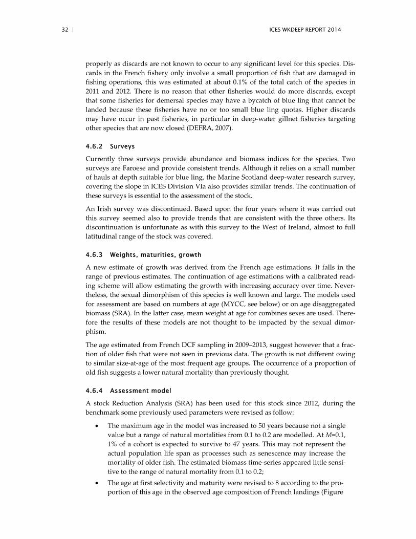
4.6.3 Weights, maturities, growth
A new estimate of growth was derived from the French age estimations. It falls in the range of previous estimates. The continuation of age estimations with a calibrated read-ing scheme will allow estimating the growth with increasing accuracy over time. Never-theless, the sexual dimorphism of this species is well known and large. The models used for assessment are based on numbers at age (MYCC, see below) or on age disaggregated biomass (SRA). In the latter case, mean weight at age for combines sexes are used. There-fore the results of these models are not thought to be impacted by the sexual dimor-phism.
The age estimated from French DCF sampling in 2009–2013, suggest however that a frac-tion of older fish that were not seen in previous data. The growth is not different owing to similar size-at-age of the most frequent age groups. The occurrence of a proportion of old fish suggests a lower natural mortality than previously thought.
4.6.4 Assessment model
A stock Reduction Analysis (SRA) has been used for this stock since 2012, during the benchmark some previously used parameters were revised as follow:
• The maximum age in the model was increased to 50 years because not a single value but a range of natural mortalities from 0.1 to 0.2 are modelled. At M=0.1, 1% of a cohort is expected to survive to 47 years. This may not represent the actual population life span as processes such as senescence may increase the mortality of older fish. The estimated biomass time-series appeared little sensi-tive to the range of natural mortality from 0.1 to 0.2;
• The age at first selectivity and maturity were revised to 8 according to the pro-portion of this age in the observed age composition of French landings (Figure
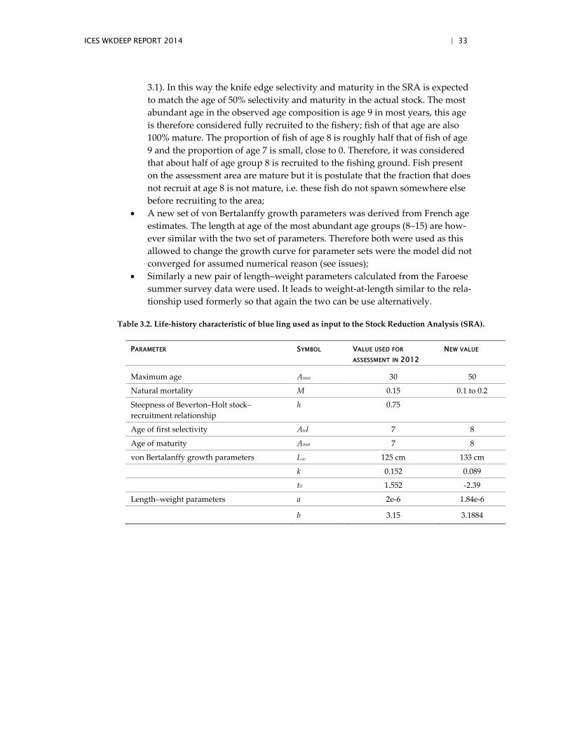
ICES WKDEEP REPORT 2014 | 33
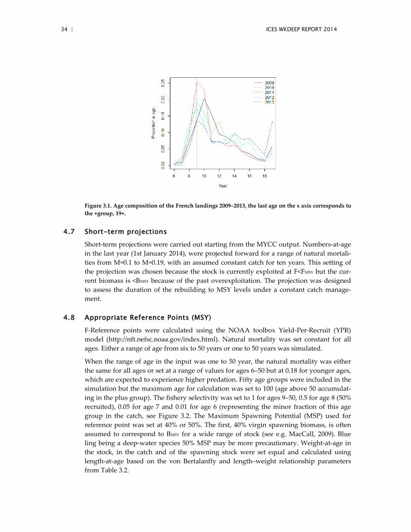
3.1). In this way the knife edge selectivity and maturity in the SRA is expected to match the age of 50% selectivity and maturity in the actual stock. The most abundant age in the observed age composition is age 9 in most years, this age is therefore considered fully recruited to the fishery; fish of that age are also 100% mature. The proportion of fish of age 8 is roughly half that of fish of age 9 and the proportion of age 7 is small, close to 0. Therefore, it was considered that about half of age group 8 is recruited to the fishing ground. Fish present on the assessment area are mature but it is postulate that the fraction that does not recruit at age 8 is not mature, i.e. these fish do not spawn somewhere else before recruiting to the area;
• A new set of von Bertalanffy growth parameters was derived from French age estimates. The length at age of the most abundant age groups (8–15) are how-ever similar with the two set of parameters. Therefore both were used as this allowed to change the growth curve for parameter sets were the model did not converged for assumed numerical reason (see issues);
• Similarly a new pair of length–weight parameters calculated from the Faroese summer survey data were used. It leads to weight-at-length similar to the rela-tionship used formerly so that again the two can be use alternatively.
Table 3.2. Life-history characteristic of blue ling used as input to the Stock Reduction Analysis (SRA).
PARAMETER SYMBOL VALUE USED FOR
ASSESSMENT IN 2012 NEW VALUE
Maximum age Amax 30 50
Natural mortality M 0.15 0.1 to 0.2
Steepness of Beverton–Holt stock–recruitment relationship
h 0.75
Age of first selectivity Asel 7 8
Age of maturity Amat 7 8
von Bertalanffy growth parameters L∞ 125 cm 133 cm
k 0.152 0.089
t0 1.552 -2.39
Length–weight parameters a 2e-6 1.84e-6
b 3.15 3.1884
34 | ICES WKDEEP REPORT 2014
Figure 3.1. Age composition of the French landings 2009–2013, the last age on the x axis corresponds to the +group, 19+.
4.7 Short-term projections
Short-term projections were carried out starting from the MYCC output. Numbers-at-age in the last year (1st January 2014), were projected forward for a range of natural mortali-ties from M=0.1 to M=0.19, with an assumed constant catch for ten years. This setting of the projection was chosen because the stock is currently exploited at F<FMSY but the cur-rent biomass is <BMSY because of the past overexploitation. The projection was designed to assess the duration of the rebuilding to MSY levels under a constant catch manage-ment.
4.8 Appropriate Reference Points (MSY)
F-Reference points were calculated using the NOAA toolbox Yield-Per-Recruit (YPR) model (http://nft.nefsc.noaa.gov/index.html). Natural mortality was set constant for all ages. Either a range of age from six to 50 years or one to 50 years was simulated.
When the range of age in the input was one to 50 year, the natural mortality was either the same for all ages or set at a range of values for ages 6–50 but at 0.18 for younger ages, which are expected to experience higher predation. Fifty age groups were included in the simulation but the maximum age for calculation was set to 100 (age above 50 accumulat-ing in the plus group). The fishery selectivity was set to 1 for ages 9–50, 0.5 for age 8 (50% recruited), 0.05 for age 7 and 0.01 for age 6 (representing the minor fraction of this age group in the catch, see Figure 3.2. The Maximum Spawning Potential (MSP) used for reference point was set at 40% or 50%. The first, 40% virgin spawning biomass, is often assumed to correspond to BMSY for a wide range of stock (see e.g. MacCall, 2009). Blue ling being a deep-water species 50% MSP may be more precautionary. Weight-at-age in the stock, in the catch and of the spawning stock were set equal and calculated using length-at-age based on the von Bertalanffy and length–weight relationship parameters from Table 3.2.
ICES WKDEEP REPORT 2014 | 35
For all YPR simulations, F0.1 and FMAX were larger than F40%MSP and F50%MSP. F40%MSP was only slightly smaller than M, which is unusual, as F producing 35 to 40% SPR is usually in the order of 0.8*M. F40%MSP was even higher than M for M=0.18. This may reflects that for this stock, the fishing mortality only applies to adult fish. The F40%MSP =0.8*M rule of thumb might be derived from shelf demersal stock, were some fishing mortality of juve-niles and pre-mature occurs.
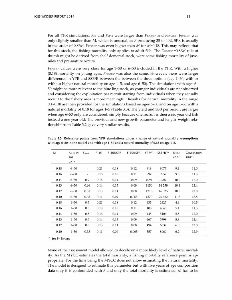
F40%MSP values were very close for age 1–50 or 6–50 included in the YPR. With a higher (0.18) mortality on young ages, F40%MSP was also the same. However, there were larger differences in YPR and SSB/R between the between the three options (age 1–50, with or without higher natural mortality on age 1–5, and age 6–50). The simulations with ages 6–50 might be more relevant to the blue ling stock, as younger individuals are not observed and considering the exploitation par recruit starting from individuals when they actually recruit to the fishery area is more meaningful. Results for natural mortality in the range 0.1–0.18 are then provided for the simulations based on ages 6–50 and on age 1–50 with a natural mortality of 0.18 for ages 1–5 (Table 3.3). The yield and SSB per recruit are larger when age 6–50 only are considered, simply because one recruit is then a six year old fish instead a one year old. The previous and new growth parameter and length–weight rela-tionship from Table 3.2 gave very similar results.
Table 3.3. Reference points from YPR simulations under a range of natural mortality assumptions with age 6–50 in the model and with age 1–50 and a natural mortality of 0.18 on age 1–5.
M AGES IN
THE
DATA
FMAX F-01 F 40%SPR F 50%SPR YPR(1) SSB/R(1) MEAN
AGE(1) GENERATION
TIME(1)
0.18 6–50 - 0.21 0.18 0.12 918 8077 9.1 11.0
0.16 6–50 - 0.18 0.16 0.11 997 9957 9.5 11.5
0.14 6–50 0.9 0.16 0.14 0.09 1094 12560 10.0 12.0
0.13 6–50 0.66 0.14 0.13 0.09 1150 14 259 10.4 12.4
0.12 6–50 0.51 0.13 0.11 0.08 1213 16 325 10.8 12.8
0.10 6–50 0.33 0.11 0.09 0.065 1370 26 622 11.8 13.8
0.18 1–50 0.5 0.21 0.18 0.12 435 2627 4.6 10.5
0.16 1–50 0.5 0.18 0.16 0.11 408 4048 5.1 11.5
0.14 1–50 0.5 0.16 0.14 0.09 445 5106 5.5 12.0
0.13 1–50 0.5 0.14 0.13 0.09 467 5798 5.8 12.4
0.12 1–50 0.5 0.13 0.11 0.08 494 6637 6.0 12.8
0.10 1–50 0.33 0.11 0.09 0.065 557 8960 6.2 12.9
(1) for F= F50%SPR.
None of the assessment model allowed to decide on a more likely level of natural mortal-ity. As the MYCC estimates the total mortality, a fishing mortality reference point is ap-propriate. For the time being the MYCC does not allow estimating the natural mortality. The model is designed to estimate this parameter but with five years of age composition data only it is confounded with F and only the total mortality is estimated, M has to be
36 | ICES WKDEEP REPORT 2014
fixed. However, the model results are in accordance with the understanding that natural mortality of blue ling is smaller or equal to 0.2, with the fit degrading for M fixed at 0.19. This arises for high levels of M forcing the model to estimated high numbers in the stock to allow for some catch with a low F (as the MYCC model estimates Z if M is fixed high, F must be low).
4.9 Future research and data requirements
Data to monitor and assess this stock are now collected on a regular basis and the priority should be given to the continuation of current monitoring programmes. Two areas where progress can be made are the stock identity and the validation of age estimations.
The age estimation protocol and reading scheme were reviewed by WKAMDEEP in Oc-tober 2013. An image analysis system for measuring annuli and a standardised protocol are used for age estimations of the French samples. Calibrated and annotated otoliths images are used to maintain the same reading scheme over time. Therefore the estima-tions are expected consistent but they remain unvalidated. Options for age validation of blue ling should be considered. Further, age estimation for other countries would be use-ful first because the Faroese catches represent about 1/3 of the total catch but also because this would allow for calibration workshops and otolith exchanges between readers. Un-der appropriate calibration of age estimations, comparison of length-at-age could be made more rigorously than in the past and this could also allow revisiting the stock iden-tity.
The stock identity deserves being clarified. It seems extremely unlikely that nursery have passed unnoticed in ICES Subareas VI and VII and Division Vb. Therefore, recruits to the stock come from out of these regions. This does not preclude blue ling for ICES Subareas VI and VII and Division Vb to be assessed as a stock. In this stock unit, fish recruit mostly at an age of eight and nine and there is no indication that adult blue ling further emi-grates from the area. Therefore the stock assessment based on catch curve of adults, esti-mation of recruitment at age 8–9 and modelling of the dynamics of these adult fish is fully appropriate.
The situation raises further a number of biological and even hydrological questions:
• do eggs and larvae emitted from nursery areas in the stock assessment area reach nursery areas out of the assessment area?
• does Icelandic insular shelf represent the only significant nursery for this spe-cies in the NEA?
• which currents/waters mass movements carry eggs and larvae to these nurse-ries?
4.10 External Reviewers comments
The assessment of Blue ling in ICES Areas V, VI and VII is based on three steps. A multi-year catch curve model (MYCC) is used to estimate the total annual mortality taking into account annual variations in recruitment, a stock reduction analysis (SRA) is used to pre-dict the biomass dynamics of the stock, and a yield-per-recruit model is used to estimate reference points. The approach was deemed appropriate for assessing this species.
ICES WKDEEP REPORT 2014 | 37
Future work should be directed at combining all available information within one as-sessment method, such as XSA, rather than the current approach which pieces together the information using three assessment techniques. A further suggestion during the workshop was to use Stock Synthesis (SS3, see http://nft.nefsc.noaa.gov/), which could allow integrating the 20 years of length distribution data in the model.
4.11 References Bergstad, O. A. 1991. Distribution and trophic ecology of some gadoid fish of the Norwegian Deep.
1 Accounts of individual species. Sarsia 75:269–313.
DEFRA. 2007, Report of the results from UK observer trips in the western gillnet fishery for an-glerfish. DEFRA, London, 15 pp.
Heymans J.J., Howell K.L., Ayers M., Burrows M.T., Gordon J.D.M., Jones E.G., Neat F. 2011, Do we have enough information to apply the ecosystem approach to management of deep-sea fisheries? An example from the West of Scotland. ICES Journal of Marine Science 68, 265–280.
Lorance, P., L. Pawlowski, and V. M. Trenkel. 2010. Standardizing blue ling landings per unit effort from industry haul-by-haul data using generalized additive models. ICES Journal of Marine Science 67:1650–1658.
MacCall, A. D. 2009. Depletion-corrected average catch: a simple formula for estimating sustainable yields in data-poor situations. Ices Journal of Marine Science 66 (10), 2267–2271.10.1093/icesjms/fsp209
ICES. 2012. Report of the working group on biology and assessment of deep-sea fisheries resources (WGDEEP), 28 March–5 April 2012. International Council for the Exploration of the Sea (ICES), Copenhagen, Denmark.
38 | ICES WKDEEP REPORT 2014
5 WKDEEP Conclusions
5.1 External Reviewers’ comments on blue ling
The assessment of blue ling in ICES Areas V, VI and VII is based on three steps. A multi-year catch curve model (MYCC) is used to estimate the total annual mortality taking into account annual variations in recruitment, a stock reduction analysis (SRA) is used to pre-dict the biomass dynamics of the stock, and a yield-per-recruit model is used to estimate reference points. The approach was deemed appropriate to assessing this species.
Future work should be directed at combining all available information within one as-sessment method, such as XSA, rather than the current approach which pieces together the information using three assessment techniques.
5.2 External Reviewers’ comments on ling
The data and assessment model presented for the ling assessment for Area Va was pre-sented thoroughly by MRI scientists with complete documentation provided in advance to the review team prior to the meeting. This was an important step that contributed to the success of the benchmark workshop for this stock. The data available were well doc-umented and reflects the care taken by MRI scientists to provide the necessary infor-mation for the assessment team to conduct a thorough review of input data.
Three things can be highlighted regarding the available data. The two surveys conducted by MRI in spring and autumn are critical for the assessment of this stock. Although not originally designed for ling they have proven to be the cornerstone of the assessment together with the data from the fishery. These surveys are unusual in that they are based on an initial stratified random selection of stations, however, once selected these original stations are fished every year. Although such design is not strictly speaking stratified random sampling every year, it has the advantage of allowing a better representation of spatial changes in the distribution of stocks. Given the recent changes in the distribution of ling observed in the last decade, it seems that the decision to use stations as fixed sta-tions was, at least for ling, a wise decision. The large number of stations sampled sup-ports also the argument that these surveys produce reliable indices of abundances for ling, at least for the larger length classes (during the meeting it was concluded that indi-ces for the smallest size groups may have created the retrospective patterns in fishing mortality observed in the results).
The recent restart of the program of collection of ling age samples has clearly benefited and enriched the information available for assessment. It is essential that this programme be maintained so as to reduce the uncertainty in the estimations of stock status. It is pos-sible that a focus on ageing the smallest fish in the survey catch may help reduce the un-certainty associated with estimates of recruitment. Estimates based on catch rates of the smallest size ranges prove to be unreliable during the recent period of high recruitment. This could be the result of many things but one possible reason could be that small fish have variable growth rates and therefore that in different years the same length groups may represent different age groups. Understanding whether ling does show variable growth at young ages may therefore help reduce uncertainty in estimates of recruitment.
ICES WKDEEP REPORT 2014 | 39
The assessment model used, GADGET, is very flexible in its ability to integrate different types of data and able to cope also with various levels of data availability. It seems well suited for the assessment of ling. Its power to explicitly model length distributions and to do so by length transition matrices allows it to make changes in the length distribution to persist between subsequent time periods, something that other models that redistribute lengths between subsequent time periods cannot do. Whether such ability is critical for the assessment of ling is unclear. If it was proven that variable growth rates are an im-portant characteristic of the dynamics of this stock or that selectivity does alter the length distribution of cohorts by preferentially removing the fast growing fish, then GADGET would be a superior model to use compared with others like SS. On the other hand GADGET has very long running times compared to SS. The complexity of the GADGET model and its required run time limited our ability to conduct and review a thorough sensitivity analysis of the model to different assumptions or input data during the benchmark meeting. If this model is to be used in future benchmarks for this stock, the review panel suggests that a more thorough sensitivity analysis be conducted prior to the meeting enabling its review during the meeting.
5.3 External Reviewers’ comments on black scabbardfish
The assessment of the black scabbardfish stock in ICES Areas V, VI, VII and IX was con-ducted using a coupled Bayesian state–space model for the British Isles and mainland Portugal. The review panel considers the model appropriate to addressing the migration of the species between these two areas but is concerned that the Madeira component of the stock is omitted from the model. The review panel believes that extra effort should be put into clarifying and quantifying the migratory behaviour of the species and incorpo-rating as many data as possible from the Madeira fishery. Our understanding of the as-sessment and its results would also benefit from a more robust sensitivity analysis of the model to its assumptions and input data.
5.4 Conclusions
WKDEEP was a successful benchmark process, producing improved stock assessments across the board.
The ling assessment had previously implemented the GADGET stock assessment model on an exploratory basis only, producing a single, best-case model run. At the current benchmark, the model was implemented fully, including the addition of bootstrapped estimates of uncertainty and sensitivity analyses, and the development of a harvest con-trol rule. As a result, the ICES categorization of the stock moved from category 3 to cate-gory 1.
The blue ling assessment incorporated updated information on selectivity and longevity into its stock reduction analysis (SRA) model. There was a consensus decision to use F40 from the yield-per-recruit (YPR) analysis as a reference point to compare with the F esti-mated from the multiyear catch curve (MYCC). A control rule was developed using the three assessment methods presented (SRA, YPR, MYCC) that includes both biomass and exploitation rate components. The potential exists to conduct short-term stock projec-tions. As a result, the potential exists to change the ICES categorization of the stock from category 2 to category 1 in the near future.
40 | ICES WKDEEP REPORT 2014
The black scabbardfish assessment model developed to the point where it could be used for assessment. The benchmark participants agreed that the three original stocks should be treated as one, and the assessment model reflected this, taking into account stock structure and movement. This was the first time the stock was benchmarked. As a result, the ICES categorization of the stock moved from category 3 to category 2.
Process comments
WKDEEP was the fifth ICES benchmark in which Dr Berkson has served as external chair. There are clear lessons regarding the benchmark process that can be drawn from the success of WKDEEP.
In contrast to previous benchmarks experienced, most of the preparation required was completed prior to arriving at the benchmark. Data had been compiled, draft assessments had been completed, and requested presentations had for the most part been compiled. Engaged and active participation in the November data compilation workshop set the stage for a successful benchmark.
A reasonable number of stocks were assigned, given the time available to the benchmark. Five stocks were assigned. The benchmark participants agreed that three stocks of the same species should be treated as a single stock during the benchmark, reducing the number of stocks being benchmarked to a total of three, making the benchmark’s objec-tives even more reasonable.
The individuals responsible for producing the stock assessment analyses attended the meeting. In addition, all meeting participants were present when the meeting began and stayed until the meeting was over, rather than arriving a day late and/or departing a day early. This may seem like a trivial point, but this has not always been the case in previous benchmarks experienced.
The external reviewers were impressed at the efforts made by the stock coordinators to clearly and effectively present their assessments, address questions and concerns raised, and complete requested analyses.
ICES staff members assigned to the benchmark were highly knowledgeable, competent, and helpful, as has been the case in all prior benchmarks experienced. Their professional-ism maintains a high standard difficult to equal in other fisheries forums.
Overall this indicates that the ICES benchmark process can be successful, a statement that the External Chair would not have made as strongly in the past. Given a reasonable as-signment (not too many stocks), adequate preparation by all participants, and a signifi-cant priority and commitment placed on the completion of the work by all participants, the probability of a successful benchmark can be maximized. Should any of these factors not be present, the probability declines significantly.
The external reviewers made a number of suggestions as to how ICES could continue to improve the benchmark process.
Two alternatives were offered regarding organization of benchmarks. At WKDEEP three very different assessment methodologies were presented for the three stocks being re-viewed, requiring the external reviewers to become familiar with the theory behind each, if not already known, as well as how each method was implemented. It was suggested
ICES WKDEEP REPORT 2014 | 41
that benchmarks could be organized based on common methodology, rather than species similarity. This would allow the external reviewers to focus on one primary method at a benchmark, allowing the process to be more focused. This approach clearly has potential drawbacks, as reviewing species with common life histories, habitats, niches, ecologies, etc., provides a strong basis for interpretation of assessment assumptions and inferences.
An alternative approach would be to host methodological assessment reviews, in which external reviewers would review key datasets, data analysis methods, and/or assessment methods. For example, external reviewers could review a particular assessment model and conclude that the model would be considered appropriate to drawing specific infer-ences when certain types of data are available and particular assumptions are valid. Once this determination is made, assessments would only need to be reviewed to ensure the methods were being used appropriately. This would largely shift the benchmark process from the review of individual assessments (output) to the review of specific data and methods (input and methods) used across assessments. Given the fact that our datasets and methods are currently undergoing a period of significant diversification, an input- and methods-based benchmark process may be preferable to, or as an alternative, a good complement to, a process solely based on output review.
42 | ICES WKDEEP REPORT 2014
6 Stock annexes
6.1 Black scabbardfish stock annex
Stock specific documentation of standard assessment procedures used by ICES.
Stock Black scabbard fish in Subareas Vb and XIIb and Di visions VI and VII
Working Group WGDEEP
Date February of 2014
Revised by WKDEEP-2014 / Ivone Figueiredo
A. General
A.1. Distribution
Black scabbardfish Aphanopus carbo Lowe, 1839 is a widely distributed species. In the North Atlantic, the species occurs between 30oN and 70oN, from the strait of Denmark to Western Sahara, with greatest abundance to the South of the Faroe Islands, in the Rockall Trough, to the west of mainland Portugal, and around Madeira and the Canary archipel-agos. It occurs only sporadically north of the Scotland-Iceland-Greenland ridges.
Black scabbardfish is a bathypelagic species which can be found at depths from 200 m, in the northern section of the NE Atlantic (Nakamura and Parin, 1993; Kelly et al., 1998), to 2300 m around the Canary Islands (Pajuelo et al., 2008). Despite this wide bathymetric range, it is more frequent between 800 and 1800 m in mainland Portugal (Martins et al., 1987), 800 and 1300 m in Madeira (Morales-Nin and Sena-Carvalho, 1996), and 400 and 1400 m of the West of the British Isles (Ehrich, 1983; Allain et al., 2003).
A.2. Species dynamics
Mean length and maximum length of black scabbardfish caught west of the British Isles are smaller than those caught off mainland Portugal, which in turn are smaller than those caught in Madeira. Mature or spawning individuals have never been recorded west of the British Isles or Mainland Portugal and the only known spawning locations are around Madeira, the Canary Islands the NW coast of Africa (Figueiredo et al., 2003; Pa-juelo et al., 2008; Perera, 2008; Neves et al., 2009). Evidence from otolith microchemistry and stable isotope analysis are consistent with the fish caught west of the British Isles and Portugal having been spawned at latitudes similar to Madeira.
This leads to the hypothesis of migratory behaviour mostly driven by feeding and repro-duction processes (Zilanov and Shepel, 1975; Anon, 2000; Figueiredo et al., 2003). Accord-ing to this, spawning apparently occurs around Madeira, the Canary Islands and possibly in a few other southern areas, such as the NW coast of Africa (Figueiredo et al., 2003; Pa-juelo et al., 2008; Perera, 2008; Neves et al., 2009). Juveniles migrate from those areas to the northernmost ones, namely Iceland, the Faroes Islands, and the west of the British Isles, where small fish of about two years old have been caught by fisheries or by surveys. This northward migration also includes non-recruited stages up to a length of 70 cm. After having grown in northern areas for a few years, fish move southwards, namely to main-
ICES WKDEEP REPORT 2014 | 43
land Portugal (International Council for the Exploration of the Seas Division IXa) where they remain a few years before migrating further south to the spawning areas.
A.3. Stock definition
Although the stock structure is uncertain, in the absence of clear scientific evidence to suggest structuring it is hypothesised that a single stock exists in the NE Atlantic. Results from several studies are in agreement with this hypothesis. However, due to the differing nature of fisheries in the northern and southern areas, ICES has historically given sepa-rate advice for three assessment units. These assessment units are generally consistent with the management units used by the EU:
i ) Northern (Divisions Vb and XIIb and Subareas VI and VII); ii ) Southern (Subareas VIII and IX); iii ) Other areas (Divisions IIIa and Va Subareas I, II, IV, X, and XIV).
These management units reflect the main fisheries to which the species is subjected. The Northern component comprises fish exploited mainly by trawl fisheries while the south-ern component by a longline fishery. In other areas the species is exploited by both long-liners and trawlers, but the overall landings are very small compared with the other two management units.
In 2012, ICES Stock Identification Methods Working Group (SIMWG) recommended that the management units of Northern and Southern divisions may need revision and should be considered as one assessment unit (ICES, 2012). Consequently, a single assessment unit is now considered for this stock.
A.4. Fisheries
The Faroese fisheries take mostly place in Subarea Vb with minor activity in Subarea VI. The Faroese deep-sea trawl fishery started in the late 1970s as a mixed redfish, blue ling, grenadier and black scabbardfish fishery; a more directed black scabbard fishery began in the late 1980s (1988) as a result of improvements of the gear and handling of the fish. From 1993 onwards some of the otter board trawlers have targeted black scabbardfish either seasonally or throughout the year. The main fishing grounds for the species are located in the bank area southwest of the Faroes Islands. The fleet of otter board trawlers (the so called deep-sea trawlers) consist of 13 vessels >1000 HP, but only 1–3 trawlers >2000 HP are targeting black scabbardfish. Landings are mostly derived from Division Vb and the values (about 1400 t) were registered in 2001 and 2002.
In ICES Subarea VI a Scottish mixed deep-water trawl fishery included some catches of black scabbard fish since 1995. This fishery has decreased to low levels since the intro-duction of TACs in 2003.
Following the decline of target orange roughy Irish trawl fishery, landings of black scab-bardfish derived from ICES Subareas VI and VII reached about 1000 t in 2002. In the re-cent years (since 2008) Irish landings have been zero.
The French deep-water fishery operates mainly in Subareas VI and VII targeting round-nose grenadier, black scabbardfish, and blue ling. Over recent years, the landings of black
44 | ICES WKDEEP REPORT 2014
scabbardfish have declined but to a lesser extent than landings of other deep-water spe-cies (roundnose grenadier, blue ling, orange roughy and deep-water sharks).
The Spanish fishery in Hatton Bank started in 1996, triggered by the decline in catches in traditional fishing grounds. Durán Muñoz and Román Marcote (2001) described the be-ginning of this fishery and the fleet operating in Hatton. A total of 48 vessels have logged in fishing days at Hatton for the period 2002–2009, but the maximum number of vessels in the fishing grounds in any given month is 16. Most often, and on average, vessels stayed in Division VIb less than two weeks per month, but stayed in Division XII be-tween three and four weeks.
Total landings from the ICES Subareas Vb and Divisions VI, VII and XII show a markedly increasing trend from 1999 to 2002 followed by a decreasing trend till 2005. There was a peak in 2006 and then there was a decrease mainly due continuous decreases of landings from ICES Divisions VI and VII.
In Subarea IXa the main fishery taking place is derived from the Portuguese longliners. In the early 1980s, an artisanal longline fishery targeting this species initiated in Portuguese continental waters. The fishery takes place at grounds around Sesimbra (south of Lisboa, Latitude 38°20’ N), following a series of exploratory surveys conducted by the Portu-guese Institute of the Sea and Atmosphere (former IPIMAR) in close collaboration with professionals from the fisheries sector some of them from Madeira. These surveys were oriented towards the search for new fishing grounds for the species, the environmental characterization of the ocean layer where black scabbardfish occurs, the experimentation of longline fishing gears and preliminary studies on the biology of the species. Fishermen from Madeira with extensive experience in deep-sea longline fishing have greatly con-tributed.
The fishing method and gear used by the black scabbardfish longline fleet were devel-oped soon after the initial fishing trials off the Sesimbra coast by fishermen from Madei-ra. Gear design has been modified from the one initially used (similar to the Madeira traditional longline fishing gears) to catch the species in continental waters with a differ-ent configuration; setting horizontal bottom longline, where alternating floats and sinkers occur at constant intervals on the main line. This rearrangement aims to match the intri-cate vertical distribution exhibited by the species in the slopes and to prevent gear loss on the hard grounds (Henriques, 1997).
At the beginning of the fishery, the fleet was composed of small artisanal vessels with an average LOA around 11 m and an average tonnage of ca. 16 GRT. In 1988, there was a slight increase in both size and engine’s power of vessels. However, from 1992 to 1995, average LOA and engine’s power characteristics registered the highest raise in relation to 1988; about 30%. In 2000, the fleet again underwent technological improvements, includ-ing an increase in engine power, tonnage and average LOA average. Such improvements were experienced by a limited number of vessels (4), which is reflected by the increase in standard deviation estimates.
The number of vessels in the fleet registered its highest value in 1986, but decreased from 1995 to 2004, when the fleet presented the same number of vessels exhibited twenty years before. In the period 1995–2004, the number of new vessels that entered the fleet attained its maximum in 1997 before an equal number of vessels left the fleet in 1998. During the
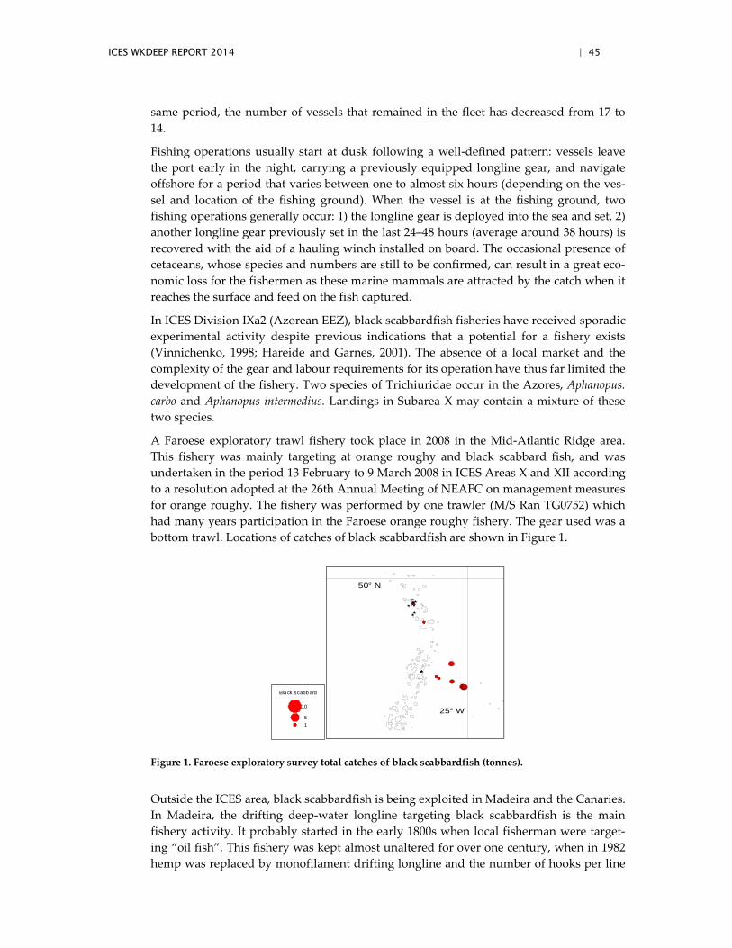
ICES WKDEEP REPORT 2014 | 45
same period, the number of vessels that remained in the fleet has decreased from 17 to 14.
Fishing operations usually start at dusk following a well-defined pattern: vessels leave the port early in the night, carrying a previously equipped longline gear, and navigate offshore for a period that varies between one to almost six hours (depending on the ves-sel and location of the fishing ground). When the vessel is at the fishing ground, two fishing operations generally occur: 1) the longline gear is deployed into the sea and set, 2) another longline gear previously set in the last 24–48 hours (average around 38 hours) is recovered with the aid of a hauling winch installed on board. The occasional presence of cetaceans, whose species and numbers are still to be confirmed, can result in a great eco-nomic loss for the fishermen as these marine mammals are attracted by the catch when it reaches the surface and feed on the fish captured.
In ICES Division IXa2 (Azorean EEZ), black scabbardfish fisheries have received sporadic experimental activity despite previous indications that a potential for a fishery exists (Vinnichenko, 1998; Hareide and Garnes, 2001). The absence of a local market and the complexity of the gear and labour requirements for its operation have thus far limited the development of the fishery. Two species of Trichiuridae occur in the Azores, Aphanopus. carbo and Aphanopus intermedius. Landings in Subarea X may contain a mixture of these two species.
A Faroese exploratory trawl fishery took place in 2008 in the Mid-Atlantic Ridge area. This fishery was mainly targeting at orange roughy and black scabbard fish, and was undertaken in the period 13 February to 9 March 2008 in ICES Areas X and XII according to a resolution adopted at the 26th Annual Meeting of NEAFC on management measures for orange roughy. The fishery was performed by one trawler (M/S Ran TG0752) which had many years participation in the Faroese orange roughy fishery. The gear used was a bottom trawl. Locations of catches of black scabbardfish are shown in Figure 1.
Figure 1. Faroese exploratory survey total catches of black scabbardfish (tonnes).
Outside the ICES area, black scabbardfish is being exploited in Madeira and the Canaries. In Madeira, the drifting deep-water longline targeting black scabbardfish is the main fishery activity. It probably started in the early 1800s when local fisherman were target-ing “oil fish”. This fishery was kept almost unaltered for over one century, when in 1982 hemp was replaced by monofilament drifting longline and the number of hooks per line
50° N
25° W
Bla ck scabb ard
10
51
46 | ICES WKDEEP REPORT 2014
increased (Martins and Ferreira, 1995). This change in fishing gear, along with better equipped boats that helped local fisherman searching for new fishing grounds such as seamounts, significantly improving their yields (Martins and Ferreira, 1995). The fleet now exploits new areas, especially located SE of Madeira, as far as 150–200 nautical miles from the fishing port. The fishery is mostly developed inside the Madeira Exclusive Eco-nomic Zone, included in the CECAF 34.1.2 area, all year round. Sporadically fishing sets are made, by the vessels with higher autonomy in the vicinity of the Madeira EEZ.
In 1800s, the fleet was composed by about 30 small artisanal vessels (<6 m length) with low engine power. The number of vessels dedicated to this fishery peaked in 1988 with a total of 95 vessels. After that period the fleet suffer a considerable reduction, mainly be-tween 1990 and 1995, when the number of vessels dropped from 84 to 44 (Bordalo-Machado et al., 2009). Between 1998 and 2000, the fleet comprised ca. 40 vessels (on aver-age 13 m LOA, 19 GT and 150 Hp) (Reis et al., 2001). Fleet size continued to decrease to around 15 vessels in the most recent years (2009–2010), with no significant changes in their technical characteristics. Landings of black scabbardfish reached a peak of 4.2 thou-sand tonnes in 1998 and have been steadily declining since then to 1.7 thousand tonnes in 2012.
A.5. Ecosystem aspects
A large proportion of deep-water trawl catches (upwards of 50%) can consist of unpalat-able species and numerous small species, including juveniles of the target species, which are usually discarded (Allain et al., 2003). Baird's smoothhead (Alepocephalus bairdii) is the main discarded species of the trawl fishery but a large number of other non-marketable bentho-pelagic species are also discarded. The survival of these discards although un-known, it is believed to be virtually zero because of fragility of these species and the ef-fects of pressure changes during retrieval (Gordon, 2001). Therefore such fisheries have the potential to deplete the whole fish community biomass. A study of the impacts of deep-water fishing to the west of Britain using historical survey data found some evi-dence of changes in size spectra and a decline in species diversity between pre- and post-exploitation data, but the scarce and unbalanced nature of the time-series hampered firm conclusions (Basson et al., 2001).
Catch, bycatch and discards of sharks in deep-sea fisheries have been an issue of concern (Stevens et al., 2000). Deep-sea sharks are frequent bycatch of black scabbardfish longline and trawl fisheries (Clarke et al., 2005; Bordalo-Machado, 2009; Muñoz et al., 2011; Piñeiro et al., 2001) and their commercial exploitation has recently increased. It is recognized that trawls and longlines catch varied quantities of different deep-sea shark species and size frequencies in different locations (Clarke et al., 2005; Coelho et al., 2003). However, the global magnitude of the problem is still unknown. It has been recognized that the bycatch of deep-sea sharks in trawls is lower than for longlines in many locations (Piñeiro et al., 2001; Hareide & Garnes 2001; Clarke et al., 2005) but post catch survival is likely to be higher in longlining (Coelho and Erzini, 2008). Some solutions may exist to reduce deep-sea shark bycatch in longlines such as increasing the distance of the hooks from the sea-bed (Coelho et al., 2003) or use artificial baits; but still need to be tested.
The effects of fishing on the benthic habitat relates to the physical disturbance by the gear used. This includes the removal of physical features, reduction in complexity of habitat structure and resuspension of sediment. More attention has been paid to biogenic habitat
ICES WKDEEP REPORT 2014 | 47
that occurs along the slope, mainly the cold-water coral. The main reef building species is L. pertusa. Any long-lived sessile organisms that stand proud of the seabed will be highly vulnerable to destruction by towed demersal fishing gear. There are a number of docu-mented reports of damage to Lophelia reefs in various parts of the Northeast Atlantic by trawl gear where trawl scars and coral rubble have been observed (e.g. Hall- Spencer, et al., 2002). Damage can also be caused on a smaller scale by static gears such as gillnets and longlines (Grehan et al., 2003).
In Divisions VI, VII and XIIb there are a number of known areas of cold-water corals. These include the shelf break to the west and north of Scotland, Rockall Bank, Hatton Bank and the Porcupine Bank. The best known site is the Darwin Mounds, located at 1000 m to the south of the Wyville Thompson Ridge. Some of these areas have been heav-ily impacted by deep-water trawling activities in the past (Hall-Spencer, 2002; Grehan et al., 2003) but all are now closed to bottom contacting fishing gears.
The Bay of Biscay and Iberian Coast region is situated in temperate latitudes with a cli-mate that is strongly influenced by the inflow of oceanic water from the Atlantic Ocean and by the large-scale westerly air circulation which frequently contains low pressure system. The bottom topography of region is highly variable, from continental shelf to abyssal plain. Some remarkable topographic features such as seamounts, banks and submarine canyons can be found. The coastline is also highly diversified with estuaries, “rias” and wetlands, which all support extremely productive ecosystems.
In Subarea VIII there are historic records of impacts on deep-water ecosystems, in partic-ular corals (Joubin, 1922). In Division IXa sporadic information available suggests the existence of coral and sponges. The topography of the region reveals the existence of seamount and canyons usually considered as VME´s
B. Data
B.1. Commercial catch
In ICES Divisions VIb1 and XIIb the landings from Spanish trawling fleet operating on the Northern and Western Hatton Bank are available since 2004.
Landings from other fleets in the northern area are available from 1989 onwards, which is believed to correspond to the entire history of the fisheries.
Landing data from Subareas VIII and IX are available to WGDEEP. Almost all landing are derived from the Portuguese longline fishery that takes place in Subarea IXa. Data are available from 1989 which is believed to correspond to the entire history of the fishery.
Data are not currently available for fisheries outside the ICES area including Madeira and the Canaries.
DISCARDS
Discard data from Spanish bottom otter trawl métiers operating Hatton Bank (ICES Divi-sions VIb1 and XIIb) are available from the `Spanish observer Programme' carried out by the IEO since 1996. Trip was the sampling unit, being raised to fleet level using fishing effort as auxiliary variable.
48 | ICES WKDEEP REPORT 2014
Discarding information from the French fisheries west of the British Isles is collected by French observers. Discards of this species are very low comprising only individuals that are damaged.
In Division IXa the artisanal segment of the commercial fishing fleet is responsible for the largest landings’ quantities of deep-water species. The on-board discard sampling for longline Portuguese commercial fleet started in mid-2005 and is integrated in the Portu-guese Discard Sampling programme, included in the EU DCR/NP. Onboard sampling in longline commercial vessels is carried out in a monthly basis to get discards and trip in-formation.
B.2. Biological
Since 2003, French length data of back scabbardfish by depth are available based on data from on-board observations of French trawlers.
Length on data from Soviet exploratory fishing surveys at late 1970s at Lauzy Bank, An-thon-Dorn Bank and Anthon-Dorn Bank and the Hatton-Rockall Plateau showed that the size range of the species (70–130 cm with higher frequencies at lengths varying between 96–110 cm) do not greatly differ among areas (Vinnichenko et al., 2003).
In Division IXa length frequency and biological samples from Portuguese landing port at Sesimbra have been collected on a monthly basis since 2000.
LHC BEST ESTIMATE DERIVED FROM OTHER ESTIMATES
Maximum observed length
1510 mm Figueiredo et al., 2003
Fecundity, egg size etc 73-373 oocytes g-1 female (Madeira). Vitellogenic oocytes ranged from 0.60 to 1.50 mm.
Neves et al., (2009)
Ageing - Studies on age and growth on age and growth of the black scabbardfish have been carried out at different areas (Table 3).
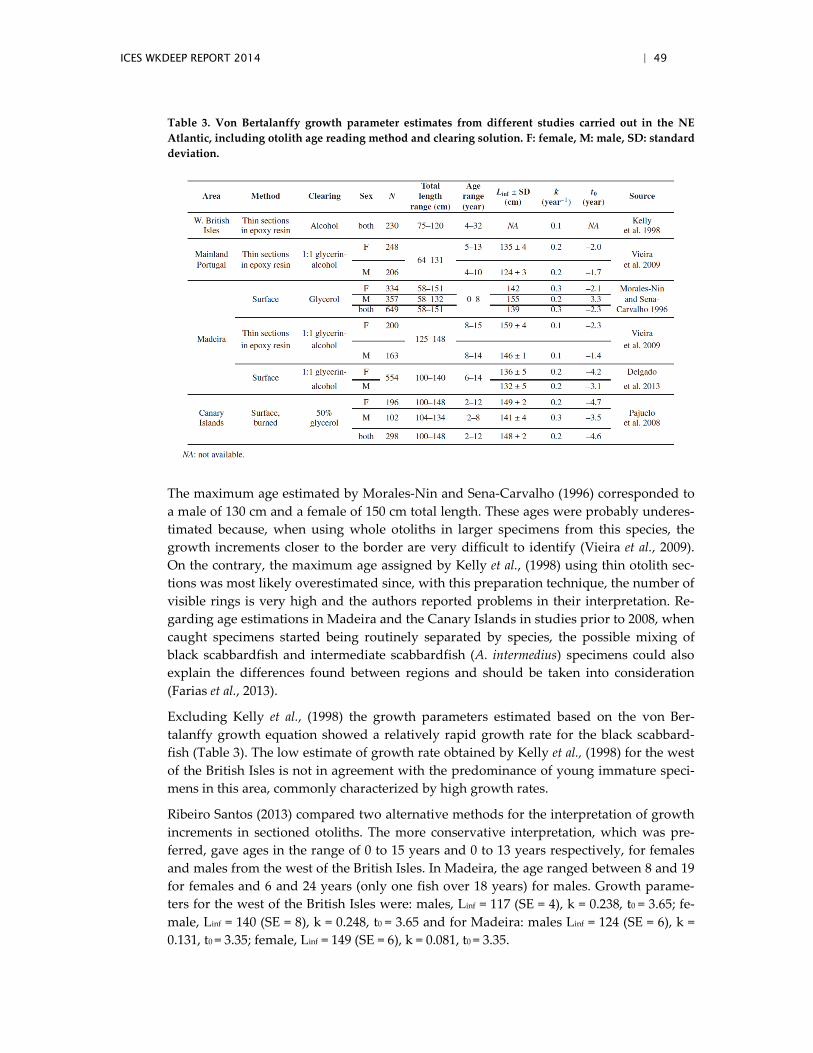
ICES WKDEEP REPORT 2014 | 49
Table 3. Von Bertalanffy growth parameter estimates from different studies carried out in the NE Atlantic, including otolith age reading method and clearing solution. F: female, M: male, SD: standard deviation.
The maximum age estimated by Morales-Nin and Sena-Carvalho (1996) corresponded to a male of 130 cm and a female of 150 cm total length. These ages were probably underes-timated because, when using whole otoliths in larger specimens from this species, the growth increments closer to the border are very difficult to identify (Vieira et al., 2009). On the contrary, the maximum age assigned by Kelly et al., (1998) using thin otolith sec-tions was most likely overestimated since, with this preparation technique, the number of visible rings is very high and the authors reported problems in their interpretation. Re-garding age estimations in Madeira and the Canary Islands in studies prior to 2008, when caught specimens started being routinely separated by species, the possible mixing of black scabbardfish and intermediate scabbardfish (A. intermedius) specimens could also explain the differences found between regions and should be taken into consideration (Farias et al., 2013).
Excluding Kelly et al., (1998) the growth parameters estimated based on the von Ber-talanffy growth equation showed a relatively rapid growth rate for the black scabbard-fish (Table 3). The low estimate of growth rate obtained by Kelly et al., (1998) for the west of the British Isles is not in agreement with the predominance of young immature speci-mens in this area, commonly characterized by high growth rates.
Ribeiro Santos (2013) compared two alternative methods for the interpretation of growth increments in sectioned otoliths. The more conservative interpretation, which was pre-ferred, gave ages in the range of 0 to 15 years and 0 to 13 years respectively, for females and males from the west of the British Isles. In Madeira, the age ranged between 8 and 19 for females and 6 and 24 years (only one fish over 18 years) for males. Growth parame-ters for the west of the British Isles were: males, Linf = 117 (SE = 4), k = 0.238, t0 = 3.65; fe-male, Linf = 140 (SE = 8), k = 0.248, t0 = 3.65 and for Madeira: males Linf = 124 (SE = 6), k = 0.131, t0 = 3.35; female, Linf = 149 (SE = 6), k = 0.081, t0 = 3.35.
50 | ICES WKDEEP REPORT 2014
Females, particularly those from Madeiran waters, had a lower growth rate than those from Mainland (ICES Subarea IXa). This reduction in the growth rate seems to be related to the reproductive effort. The differential growth pattern between the females from mainland Portugal (non-reproductive females) and Madeira (reproductive females) may reflect the optimisation of the energetic balances (Vieira et al., 2009).
Maturity - In ICES Subarea IXa only immature and early developing specimens have been observed (Figueiredo, 2009 WD). Mature individuals only occurred in Madeira (Figueiredo et al., 2003) and, in Canary Islands (Pajuelo et al., 2008) and the northwest coast of Africa although it is possible that two species may occur in these areas.
The black scabbardfish is an iteroparous species, since it can spawn multiple times throughout its life, and is also a total spawner, as it spawns in one single event (Pajuelo et al., 2008; Ribeiro Santos et al., 2013).
Mature and spawning adults have only been observed in the last quarter of the year in Madeira (Figueiredo et al., 2003; Neves et al., 2009; Ribeiro Santos et al., 2013), the Canar-ies (Pajuelo et al., 2008), and the northwest coast of Africa (Perera, 2008).
An increase in the relative weight of the liver just before the increase in weight of gonads in females was very conspicuous in Madeira, but it could also be perceived in mainland females. Such strategy is typical of thin fishes in which the majority of the energy neces-sary to maturity is stored in the liver and, after the maturation is reached, the HSI present a sharp decrease. In males, the HSI did not follow the same conspicuous pattern shown in females since the energy needed for their reproduction has lower energy costs than females’. The HSI revealed a correlation with GSI in females but not in males and no rela-tion of the Fulton’s condition factor with the reproduction in both sexes was perceived.
Length of first maturity - Estimated female length at first maturity (L50) was 103 cm around Madeira (Figueiredo et al., 2003) and 114 cm around the Canary Islands (Pajuelo et al., 2008). Once again, the possible mixture of black and intermediate scabbardfish specimens in the samples may have biased these results. In a more recent work, female L50 was estimated to be 111 cm for Madeira and 116 cm when also including specimens from the west of the British Isles (Ribeiro Santos et al., 2013). The latter values are proba-bly overestimated because the estimation did not include specimens from Madeira small-er than 92 cm in total length (Farias et al., 2013).
Fecundity - Black scabbardfish has a determinate fecundity strategy the relative fecundi-ty estimates ranged from 73 to 373 oocytes/female weights (g). Skipped spawning was also considered to occur in this species; the percentages of non-reproductive females between 21% and 37% (Vieira et al., 2009).
B.3. Surveys
Survey data on the species are available both from Scottish and Irish surveys. The former is conducted by the Marine Scotland - Science [formerly Fisheries Research Services, (FRS)] along the continental shelf/slope to the northwest of Scotland. The survey was initiated in 1996 with strictly comparable data available between 1998 and 2008. The core area is surveyed between 55–59°N, with trawling undertaken at depths ranging from 300 to 1900 m with most of the hauls being conducted at fixed stations, at depths of around 500 m, 1000 m, 1500 m and 1800 m. Further hauls have been made on seamounts in the
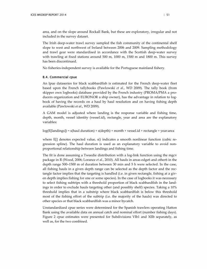
ICES WKDEEP REPORT 2014 | 51
area, and on the slope around Rockall Bank, but these are exploratory, irregular and not included in the survey dataset.
The Irish deep-water trawl survey sampled the fish community of the continental shelf slope to west and northwest of Ireland between 2006 and 2009. Sampling methodology and trawl gear were standardised in accordance with the Scottish deep-water survey with trawling at fixed stations around 500 m, 1000 m, 1500 m and 1800 m. This survey has been discontinued.
No fisheries-independent survey is available for the Portuguese mainland fishery.
B.4. Commercial cpue
An lpue dataseries for black scabbardfish is estimated for the French deep-water fleet based upon the French tallybooks (Pawlowski et al., WD 2009). The tally book (from skipper own logbooks) database provided by the French industry (PROMA/PMA a pro-ducers organization and EURONOR a ship owner), has the advantage in relation to log-book of having the records on a haul by haul resolution and on having fishing depth available (Pawlowski et al., WD 2009).
A GAM model is adjusted where landing is the response variable and fishing time, depth, month, vessel identity (vessel.id), rectangle, year and area are the explanatory variables:
log(E[landings]) = s(haul duration) + s(depth) + month + vessel.id + rectangle + year:area
where E[] denotes expected value, s() indicates a smooth nonlinear function (cubic re-gression spline). The haul duration is used as an explanatory variable to avoid non-proportional relationship between landings and fishing time.
The fit is done assuming a Tweedie distribution with a log-link function using the mgcv package in R (Wood, 2006; Lorance et al., 2010). All hauls in areas edge6 and other6 in the depth range 500–1500 m of duration between 30 min and 5 h were selected. In the case, all fishing hauls in a given depth range can be selected as the depth factor and the rec-tangle factor implies that the targeting is handled (i.e. in given rectangle, fishing at a giv-en depth implies fishing for one or some species). In the case of logbooks it was necessary to select fishing subtrips with a threshold proportion of black scabbardfish in the land-ings in order to exclude hauls targeting other (and possibly shelf) species. Taking a 10% threshold implies that in a substrip where black scabbardfish is below this threshold most of the fishing effort of the subtrip (i.e. the majority of the hauls) was directed to other species or that black scabbardfish was a minor bycatch.
Unstandardized cpue series were determined for the Spanish trawlers operating Hatton Bank using the available data on annual catch and nominal effort (number fishing days). Figure 2 cpue estimates were presented for Subdivisions VIb1 and XIIb separately, as well as, for the two combined.
52 | ICES WKDEEP REPORT 2014
Figure 2. Black scabbard fish cpue (kg/fishing days) in VIb (upper left). XIb (upper right) and the two Subareas combined (center) from Spanish trawlers.
A LPUE dataseries for black scabbardfish is estimated for the Portuguese longline fishery operating in Portugal mainland (ICES Subarea IXa). The commercial daily landings from Portuguese longline vessels are used to derive black scabbardfish monthly LPUE values. Data has been provided by the Portuguese General Directorate of Fisheries and Aquacul-ture.
Monthly LPUE are calculated for each vessel as the ratio total landed weight (kg) / num-ber of fishing trips. Only vessels having total monthly landings ≥ 1000 kg and a monthly number of fishing trips ≥ 5 were considered in the analysis.
Although there is no information on the number of hooks used per trip, it is known from interviews with the fishermen that each vessel uses the same number of hooks on each trip (Bordalo-Machado and Figueiredo, 2009). Hence, the effect of the number of hooks on the effort estimates is extracted from the model when we extract the effect of the ves-sel.
Standardized monthly LPUE is estimated based on the adjustment of GLM model. Fac-tors considered are YEAR, MONTH and VESSEL and the model is expressed as:
g(LPUEijkl) = αiYEARi + βjMONTHj + λkVESSELk + εijkl, (1)
0
100
200
300
400
500
600
2001 2002 2003 2004 2005 2006 2007 2008 2009 2010Year
CPUE(kg/fishday) XII
0
100
200
300
400
500
600
2001 2002 2003 2004 2005 2006 2007 2008 2009 2010Year
CPUE(kg/fishday) VIB
0
100
200
300
400
500
600
2001 2002 2003 2004 2005 2006 2007 2008 2009 2010Year
CPUE(kg/fishday)
ICES WKDEEP REPORT 2014 | 53
where αi (i = 1995,…, lastyear), βj (j = 1,…,12) and λk (k = 1,…,33) are coefficients to be de-termined. The most appropriate distribution the expected or a function of the expected response variable is chosen among the exponential family group of distributions. The quality of the model adjustment is evaluated by quantile residuals analysis.
B.5. Other relevant data
Information from the fishery, particularly the abundance index, cpue, indicates the exist-ence of a seasonal trend in abundance, both in BI and in P: lesser abundance is usually registered from March to August of any year (here referred as the 1st semester) and high-er abundances are mostly registered from September to December of an year and January and February of the following year (here referred as the 2nd semester). These fluctuations in abundance are considered to be associated with the migratory processes and as a con-sequence, the time unit adopted to analyse the dynamics of the population is the semes-ter defined as before and denoted by s.
C. Assessment: data and method
Data
The input data for the model are
- the number of specimens landed in each semester (defined as mentioned above) by the French trawlers and the Portuguese longliners partitioned into two length groups 70<C2<103 cm and C3>103 cm. The time-series covered is from 1999 to 2012;
- Standardized total fishing effort for each of the two fleet for the time period from 1999–2012.
The input data for the model are in turn dependent on data availability on:
- Length–frequency distributions from onboard observers from the French trawlers;
- Monthly landings of the Portuguese longline fishery by commercial longline category;
- Length–frequency distributions from landing sampling program; - Weight–length relationship; - Standardized cpue for each of the two fleets.
Model used
The model used consists of two state space models, one for part of the population in the BI and the other for part of the population in P. In both cases the state vectors are parti-tioned into four groups defined according to criteria to length size (C2 or C3) and the fishing status (fished, F, or not fished, ).
In each semester s, the population abundance in BI and in P is given, respectively, by the state vectors nBI;s and nP;s, with the following components
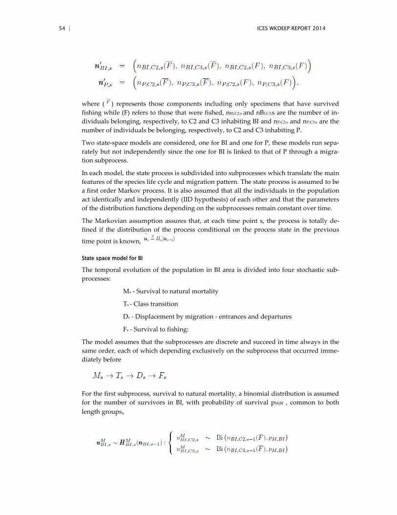
54 | ICES WKDEEP REPORT 2014
where ( ) represents those components including only specimens that have survived fishing while (F) refers to those that were fished, nBI;C2;s and nBI;C3;s are the number of in-dividuals belonging, respectively, to C2 and C3 inhabiting BI and nP;C2;s and nP;C3;s are the number of individuals be belonging, respectively, to C2 and C3 inhabiting P.
Two state-space models are considered, one for BI and one for P, these models run sepa-rately but not independently since the one for BI is linked to that of P through a migra-tion subprocess.
In each model, the state process is subdivided into subprocesses which translate the main features of the species life cycle and migration pattern. The state process is assumed to be a first order Markov process. It is also assumed that all the individuals in the population act identically and independently (IID hypothesis) of each other and that the parameters of the distribution functions depending on the subprocesses remain constant over time.
The Markovian assumption assures that, at each time point s, the process is totally de-fined if the distribution of the process conditional on the process state in the previous
time point is known,
State space model for BI
The temporal evolution of the population in BI area is divided into four stochastic sub-processes:
Ms - Survival to natural mortality
Ts - Class transition
Ds - Displacement by migration - entrances and departures
Fs - Survival to fishing:
The model assumes that the subprocesses are discrete and succeed in time always in the same order, each of which depending exclusively on the subprocess that occurred imme-diately before
For the first subprocess, survival to natural mortality, a binomial distribution is assumed for the number of survivors in BI, with probability of survival pM;BI , common to both length groups,
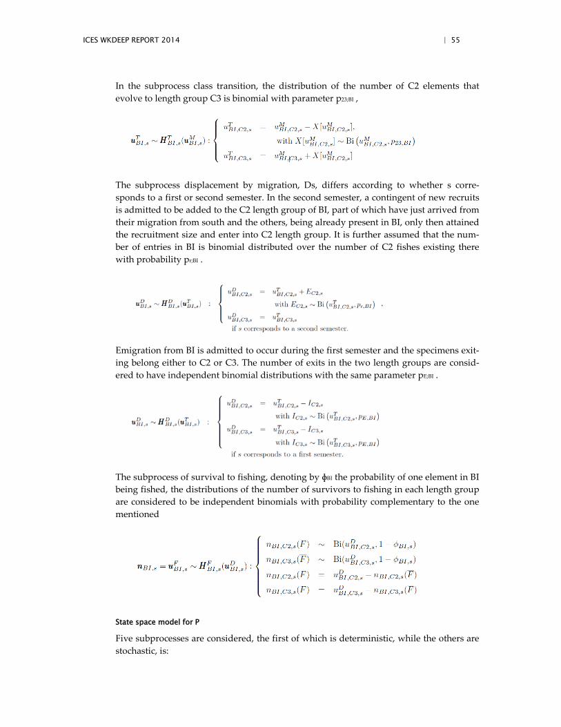
ICES WKDEEP REPORT 2014 | 55
In the subprocess class transition, the distribution of the number of C2 elements that evolve to length group C3 is binomial with parameter p23;BI ,
The subprocess displacement by migration, Ds, differs according to whether s corre-sponds to a first or second semester. In the second semester, a contingent of new recruits is admitted to be added to the C2 length group of BI, part of which have just arrived from their migration from south and the others, being already present in BI, only then attained the recruitment size and enter into C2 length group. It is further assumed that the num-ber of entries in BI is binomial distributed over the number of C2 fishes existing there with probability pr;BI .
Emigration from BI is admitted to occur during the first semester and the specimens exit-ing belong either to C2 or C3. The number of exits in the two length groups are consid-ered to have independent binomial distributions with the same parameter pE;BI .
The subprocess of survival to fishing, denoting by ɸBI the probability of one element in BI being fished, the distributions of the number of survivors to fishing in each length group are considered to be independent binomials with probability complementary to the one mentioned
State space model for P
Five subprocesses are considered, the first of which is deterministic, while the others are stochastic, is:
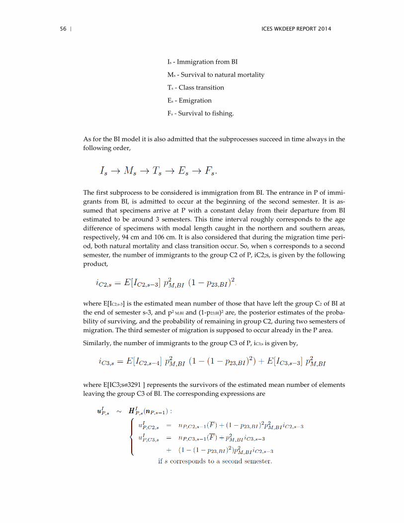
56 | ICES WKDEEP REPORT 2014
Is - Immigration from BI
Ms - Survival to natural mortality
Ts - Class transition
Es - Emigration
Fs - Survival to fishing.
As for the BI model it is also admitted that the subprocesses succeed in time always in the following order,
The first subprocess to be considered is immigration from BI. The entrance in P of immi-grants from BI, is admitted to occur at the beginning of the second semester. It is as-sumed that specimens arrive at P with a constant delay from their departure from BI estimated to be around 3 semesters. This time interval roughly corresponds to the age difference of specimens with modal length caught in the northern and southern areas, respectively, 94 cm and 106 cm. It is also considered that during the migration time peri-od, both natural mortality and class transition occur. So, when s corresponds to a second semester, the number of immigrants to the group C2 of P, iC2;s, is given by the following product,
where E[IC2;s-3] is the estimated mean number of those that have left the group C2 of BI at the end of semester s-3, and p2 M;BI and (1-p23;BI)2 are, the posterior estimates of the proba-bility of surviving, and the probability of remaining in group C2, during two semesters of migration. The third semester of migration is supposed to occur already in the P area.
Similarly, the number of immigrants to the group C3 of P, iC3;s is given by,
where E[IC3;s�3291 ] represents the survivors of the estimated mean number of elements leaving the group C3 of BI. The corresponding expressions are
ICES WKDEEP REPORT 2014 | 57
The next state processes (Survival to natural mortality, Class transition, Emigration, Sur-vival to fishing) are defined similarly to the corresponding BI subprocess but with pa-rameters assigned to P area.
The prior distributions for the parameters in the model were selected in a way that each of them incorporates as much information as available for the species. Non-informative gamma were chosen for the prior distributions of the dispersion of the observation errors as this is the common choice for dispersion parameters.
The quality of the fitting is evaluated for each model separately. For the BI model, the catch estimates for the C2 and C3 length groups, in semester s, i.e. the components of ŶBI,s are the median of the distributions of the state process vector components corresponding to the two shed subpopulations, in that semester. For the P model, the catch estimates in semester s were obtained, in the same way and are denoted by ŶPI,s. The evaluation of the model's adequacy is based on the expected deviance and also on visual inspection of the credible intervals. Contrarily to the confidence intervals, the latter are intervals in the domain of the posterior probability distributions.
Software used
The estimation of these models, both parameters and states, is done via the Bayesian par-adigm, implying non-trivial integration of these several probability density functions, which is accomplished through sequential Monte Carlo. Two state models were consid-ered in order to estimate the BI and P abundances, being estimated by sequential im-portance sampling according to Liu and West (2010) algorithm. The necessary computations were run in R.
Model Options chosen
The prior distributions for the parameters in the models were selected in a way that each of them incorporates as much information as available for the species (Table 4). Non-informative gamma were chosen for the prior distributions of the dispersion of the ob-servation errors as this is the common choice for dispersion parameters.
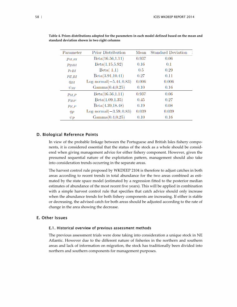
58 | ICES WKDEEP REPORT 2014
Table 4. Priors distributions adopted for the parameters in each model defined based on the mean and standard deviation shown in two right columns
D. Biological Reference Points
In view of the probable linkage between the Portuguese and British Isles fishery compo-nents, it is considered essential that the status of the stock as a whole should be consid-ered when giving management advice for either fishery component. However, given the presumed sequential nature of the exploitation pattern, management should also take into consideration trends occurring in the separate areas.
The harvest control rule proposed by WKDEEP 2104 is therefore to adjust catches in both areas according to recent trends in total abundance for the two areas combined as esti-mated by the state space model (estimated by a regression fitted to the posterior median estimates of abundance of the most recent five years). This will be applied in combination with a simple harvest control rule that specifies that catch advice should only increase when the abundance trends for both fishery components are increasing. If either is stable or decreasing, the advised catch for both areas should be adjusted according to the rate of change in the area showing the decrease.
E. Other Issues
E.1. Historical overview of previous assessment methods
The previous assessment trials were done taking into consideration a unique stock in NE Atlantic. However due to the different nature of fisheries in the northern and southern areas and lack of information on migration, the stock has traditionally been divided into northern and southern components for management purposes.
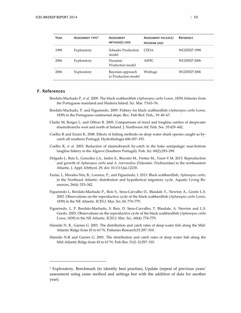
ICES WKDEEP REPORT 2014 | 59
YEAR ASSESSMENT TYPE3
ASSESSMENT
METHOD(S) USED ASSESSMENT PACKAGE/ PROGRAM USED
REFERENCE
1998 Exploratory Scheafer Production model
CEDA WGDEEP 1998
2006 Exploratory Dynamic Production model
ASPIC WGDEEP 2006
2006 Exploratory Bayesian approach to Production model
Winbugs WGDEEP 2006
F. References Bordalo-Machado P, et al. 2009. The black scabbardfish (Aphanopus carbo Lowe, 1839) fisheries from
the Portuguese mainland and Madeira Island. Sci. Mar. 73:63–76.
Bordalo-Machado, P. and Figueiredo. 2009. Fishery for black scabbardfish (Aphanopus carbo Lowe, 1839) in the Portuguese continental slope. Rev. Fish Biol. Fish., 19: 49–67.
Clarke M, Borges L. and Officer R. 2005. Comparisons of trawl and longline catches of deepwater elasmobranchs west and north of Ireland. J. Northwest Atl. Fish. Soc. 35:429–442.
Coelho R and Erzini K. 2008. Effects of fishing methods on deep water shark species caught as by-catch off southern Portugal. Hydrobiologia 606:187–193.
Coelho R, et al. 2003. Reduction of elasmobranch by-catch in the hake semipelagic near-bottom longline fishery in the Algarve (Southern Portugal). Fish. Sci. 69(2):293–299.
Delgado J., Reis S., González J.A., Isidro E., Biscoito M., Freitas M., Tuset V.M. 2013. Reproduction and growth of Aphanopus carbo and A. intermedius (Teleostei: Trichiuridae) in the northeastern Atlantic. J. Appl. Ichthyol. 29, doi: 10.1111/jai.12230.
Farias, I., Morales-Nin, B., Lorance, P., and Figueiredo, I. 2013. Black scabbardfish, Aphanopus carbo, in the Northeast Atlantic: distribution and hypothetical migratory cycle. Aquatic Living Re-sources, 26(4): 333–342.
Figueiredo I., Bordalo-Machado P., Reis S., Sena-Carvalho D., Blasdale T., Newton A., Gordo L.S. 2003. Observations on the reproductive cycle of the black scabbardfish (Aphanopus carbo Lowe, 1839) in the NE Atlantic. ICES J. Mar. Sci. 60, 774–779.
Figueiredo, I., P. Bordalo-Machado, S. Reis, D. Sena-Carvalho, T. Blasdale, A. Newton and L.S. Gordo. 2003. Observations on the reproductive cycle of the black scabbardfish (Aphanopus carbo Lowe, 1839) in the NE Atlantic. ICES J. Mar. Sci., 60(4): 774–779.
Hareide N. R., Garnes G. 2001. The distribution and catch rates of deep-water fish along the Mid-Atlantic Ridge from 43 to 61°N. Fisheries Research;51:297–310.
Hareide N-R and Garnes G. 2001. The distribution and catch rates of deep water fish along the Mid-Atlantic Ridge from 43 to 61°N. Fish Res. 51(2–3):297–310.
3 Exploratory, Benchmark (to identify best practise), Update (repeat of previous years’ assessment using same method and settings but with the addition of data for another year).
60 | ICES WKDEEP REPORT 2014
ICES. 2012. Report of the Stock Identification Methods Working Group (SIMWG), 14–16 May 2012, Manchester, UK. ICES CM 2012/SSGSUE:04. 48 pp.
Liu J., West M. 2001. Combining parameter and state estimation in simulation-based filtering. In: Doucet A., de Freitas N., Gordon N. (eds.), Sequential Monte Carlo methods in practice. New York, Springer-Verlag, pp. 197–224.
Lorance, P., Pawlowski, L. and Trenkel, V.M. 2010. Standardizing blue ling landings per unit effort from industry haul-by-haul data using generalized additive models ICES Journal of Marine Science, 67: 000–000.
Martins, M. R., M. M. Martins and F. Cardador. 1989. Portuguese fishery of Black scabbard fish (Aphanopus carbo Lowe, 1839) off Sesimbra waters. ICES Demersal Fish committee CM1989/G:38, 29 pp.
Martins, M. R., M. M. Martins and F. Cardador. 1989. Portuguese fishery of Black scabbard fish (Aphanopus carbo Lowe, 1839) off Sesimbra waters. ICES Demersal Fish committee CM1989/G:38, 29 pp.
Martins, R., C. Ferreira. 1995. Line fishing for black scabbardfish (Aphanopus carbo Lowe, 1839) and other deep water species in the eastern mid Atlantic to the north of Madeira. In A.G. Hopper (ed.). Deep-water fisheries of the North Atlantic oceanic slope. NATO ASI Series, Nederlands, pp. 323–335.
Morales-Nin, B, A. Canha, M. Casas, I. Figuereido, L.S. Gordo, J. Gordon, E. Gouveia, C.G. Pineiro, S. Reis, A. Reis and S.C. Swan. 2002. Intercalibration of age readings of deepwater black scab-bardfish, Aphanopus carbo (Lowe, 1839). ICES J. Mar. Sci., 59(2):352–364.
Muñoz PD, et al. 2011. Effects of deep-sea bottom longlining on the Hatton Bank fish communities and benthic ecosystem, north-east Atlantic. J. Mar. Biol. Assoc. UK 91(4):939–952.
Neves A., Vieira A.R., Farias I., Figueiredo I., Sequeira V., Gordo L.S. 2009. Reproductive strategies in black scabbardfish (Aphanopus carbo Lowe, 1839) from the NE Atlantic. Sci. Mar. 73S2, 19–31.
Pajuelo J.G., González J.A., Santana J.I., Lorenzo J.M., García-Mederos A., Tuset V. 2008. Biological parameters of the bathyal fish black scabbardfish (Aphanopus carbo Lowe, 1839) off the Canary Islands, Central-east Atlantic. Fish. Res. 92, 140–147.
Pajuelo JG, Gonzalez JA, and Santana JI. 2010. Bycatch and incidental catch of the black scabbard-fish (Aphanopus spp) fishery off the Canary Islands. Fish Res. 106(3):448–453.
Pajuelo, J.G., J.A. González, J.I Santana, J.M. Lorenzo, A. García-Mederos and V. Tuset. 2008. Bio-logical parameters of the bathyal fish black scabbardfish (Aphanopus carbo Lowe, 1839) off the Canary Islands, Central-east Atlantic. Fish. Res., 92(2-3): 140–147.
Perera C.B. 2008. Distribution and biology of Black scabbardfish (Aphanopus carbo Lowe, 1839) in the Northwest of Africa. Tese de Mestrado em Biologia e Gestão em Recursos Marinhos. Fac-uldade de Ciências, Lisboa.
Piñeiro CG, Casas M, and Bañón R. 2001. The deep-water fisheries exploited by Spanish fleets in the Northeast Atlantic: a review of the current status. Fish Res. 51(2):311–320.
Reis, S., D. Sena-Carvalho, J.H. Delgado, M. Afonso-Dias. 2001. Historical Overview of the black scabbardfish (Aphanopus carbo Lowe, 1839) fishery in Madeira Island. Deep-Sea Fisheries Sym-posium, NAFO SCR Doc. 01/103, 6 pp.
Ribeiro Santos A. 2013. The Life History and Ecology of Black Scabbardfish (Aphanopus carbo Lowe 1839) in the North-east Atlantic. Thesis submitted to the National University of Ireland in ful-filment of the requirements for the degree of Doctor of Philosophy. University College Cork, Ireland.

ICES WKDEEP REPORT 2014 | 61
Stefanni S., Knutsen H. 2007. Phylogeography and demographic history of the deep-sea fish, Apha-nopus carbo, in the NE Atlantic: vicariance followed by secondary contact or speciation? Molec-ular Phylogeny and Evolution; 42:38–46.
Wood S. 2006. Generalized Additive Models: An Introduction with R Chapman & Hall/CRC 410p.
62 | ICES WKDEEP REPORT 2014
6.2 Ling in Division Va stock annex
Stock specific documentation of standard assessment procedures used by ICES.
Stock Ling in Va
Working Group WGDEEP
Date February 2014
Revised by WKDEEP-2014 / Gudmundur Thordarson
A. General
A.1. Stock definition
WGDEEP 2006 indicated: ‘There is currently no evidence of genetically distinct populations within the ICES area. However, ling at widely separated fishing grounds may still be sufficiently isolated to be considered management units, i.e. stocks, between which exchange of individuals is limited and has little effect on the structure and dynamics of each unit. It was suggested that Ice-land (Va), the Norwegian Coast (II), and the Faroes and Faroe Bank (Vb) have separate stocks, but that the existence of distinguishable stocks along the continental shelf west and north of the British Isles and the northern North Sea (Subareas IV, VI, VII and VIII) is less probable. Ling is one of the species included in a recently initiated Norwegian population structure study using molecular genetics, and new data may thus be expected in the future’.
WGDEEP 2007 examined available evidence on stock discrimination and concluded that available information is not sufficient to suggest changes to current ICES interpretation of stock structure.
A.2. Fishery
The fishery for ling in Va has not changed substantially in recent years. Around 150 long-liners annually report catches of ling, around 70 gillnetters and a similar number of trawlers. Most of ling in Va is caught on longlines and the proportion caught by that gear has increased since 2000 to around 65% in 2010. At the same time the proportion caught by gillnets has decreased from 20–30% in 2000–2001 to 4–8% in 2008–2010. Catches in trawls have varied less and have been at around 20%.
Most of the ling caught in Va by Icelandic longliners is caught at depths less than 300 meters and less than 500 meters by trawlers. The main fishing grounds for ling in Va as observed from logbooks are on the south, southwestern and western part of the Icelandic shelf.
In the 1950s until 1970 the total landings of Ling in Va amounted to 10 000 to 16 000 tonnes annually of which more than half was usually caught by foreign fleets. This changed with the extension of the Icelandic EEZ in the early 1970s when total landings fell to 4000–8000 tonnes of which the Icelandic fleet caught the main share. Between 1980 and 2000 catches varied between 3200 to 5800 tonnes
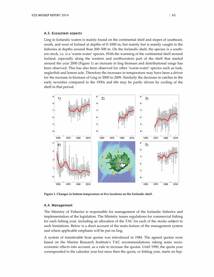
ICES WKDEEP REPORT 2014 | 63
A.3. Ecosystem aspects
Ling in Icelandic waters is mainly found on the continental shelf and slopes of southeast, south, and west of Iceland at depths of 0–1000 m, but mainly but is mainly caught in the fisheries at depths around than 200–500 m. On the Icelandic shelf, the species is a south-ern stock, i.e. is a ‘warm-water’ species. With the warming of the continental shelf around Iceland, especially along the western and northwestern part of the shelf that started around the year 2000 (Figure 1) an increase in ling biomass and distributional range has been observed. This has also been observed for other ‘warm-water’ species such as tusk, anglerfish and lemon sole. Therefore the increases in temperature may have been a driver for the increase in biomass of Ling in 2000 to 2009. Similarly the decrease in catches in the early seventies compared to the 1950s and 60s may be partly driven by cooling of the shelf in that period.
Figure 1. Changes in bottom temperature at five locations on the Icelandic shelf.
A.4. Management
The Ministry of Fisheries is responsible for management of the Icelandic fisheries and implementation of the legislation. The Ministry issues regulations for commercial fishing for each fishing year, including an allocation of the TAC for each of the stocks subject to such limitations. Below is a short account of the main feature of the management system and where applicable emphasis will be put on ling.
A system of transferable boat quotas was introduced in 1984. The agreed quotas were based on the Marine Research Institute's TAC recommendations, taking some socio-economic effects into account, as a rule to increase the quotas. Until 1990, the quota year corresponded to the calendar year but since then the quota, or fishing year, starts on Sep-
64 | ICES WKDEEP REPORT 2014
tember 1 and ends on August 31 the following year. This was done to meet the needs of the fishing industry. In 1990, an individual transferable quota (ITQ) system was estab-lished for the fisheries and they were subject to vessel catch quotas. The ITQ system al-lows free transferability of quota between boats. This transferability can either be on a temporary (one year leasing) or a permanent (permanent selling) basis. This system has resulted in boats having quite diverse species portfolios, with companies often concen-trating/specializing on particular group of species. The system allows for some but lim-ited flexibility with regards converting a quota share of one species into another within a boat, allowance of landings of fish under a certain size without it counting fully in weight to the quota, and allowance of transfer of unfished quota between management years. The objective of these measures is to minimize discarding, which is effectively banned. Since 2006/2007 fishing season, all boats operate under the TAC system.
At the beginning, only few commercial exploited fish species were included in the ITQ system, but many other species have gradually been included. Ling in Va was included in the ITQ-system in the 2001/2002 quota year.
Landings in Iceland are restricted to particular licensed landing sites, with information being collected on a daily basis time by the Directorate of Fisheries in Iceland (the en-forcement body). All fish landed has to be weighted, either at harbour or inside the fish processing factory. The information on each landing is stored in a centralized database maintained by the Directorate and is available in real time on the Internet (www.fiskistofa.is). The accuracy of the landings statistics are considered reasonable.
All boats operating in Icelandic waters have to maintain a logbook record of catches in each haul/set. The records are available to the staff of the Directorate for inspection pur-poses as well as to the stock assessors at the Marine Research Institute.
With some minor exceptions it is required by law to land all catches. Consequently, no minimum landing size is in force. To prevent fishing of small fish various measures such as mesh size regulation and closure of fishing areas are in place.
A system of instant area closure is in place for many species. The aim of the system is to minimize fishing on juveniles. An area is closed temporarily (for 2 weeks) for fishing if on-board inspections (not 100% coverage) reveal that more than a certain percentage of the catch is composed of fish less than the defined minimum length.
B. Data
B.1. Commercial catch
Icelandic ling catches in tonnes by month, area and gear are obtained from Statistical Iceland and Directorate of Fisheries. Catches are only landed in authorized ports where all catches are weighed and recorded. The distribution of catches is obtained from log-book statistic where location of each haul, effort, depth of trawling and total catch of ling is given. Logbook statistics are available since 1991. Landings of Norwegian and Faroese vessels are given by the Icelandic Coast Guard and reported to the Directorate of Fisher-ies.
Discard is banned in the Icelandic demersal fishery. Based on limited data discard rates in the Icelandic longline fishery for ling are estimated very low (<1% in either numbers or
ICES WKDEEP REPORT 2014 | 65
weight) (WGDEEP-2011, WD02). Measures in the management system such as convert-ing quota share from one species to another are used by the fleet to a large extend and this is thought to discourage discards in mixed fisheries.
B.2. Biological
Biological data from the commercial longline and trawl fleet catches are collected from landings by scientists and technicians of the Marine Research Institute (MRI) in Iceland. The biological data collected are length (to the nearest cm), sex and maturity stage (if possible since most ling is landed gutted), and otoliths for age reading. Most of the fish that otoliths were collected from were also weighted (to the nearest gramme). Biological sampling is also collected directly on board on the commercial vessels during trips by personnel of the Directorate of Fisheries in Iceland or from landings (at harbour). These are only length samples.
The general process of the sampling strategy is to take one sample of ling for every 180 tonnes landed. Each sample consists of 150 fishes. Otoliths are extracted from 20 fish which are also length measured and weighed gutted. In most cases ling is landed gutted so it not possible to determine sex and maturity. If ling is landed un-gutted, the un-gutted weight is measured and the fish is sexed and maturity determined. The remaining 130 in the sample are only length measured. Age reading of ling from commercial catches ended in 1998, the reason was uncertainty in ageing and cost saving. However ageing was resumed in 2013 and is expected to continue, the main focus being on otoliths from catches and surveys in the current year but older otoliths will be as or if resources are available.
At 60 cm around 10% of ling in Va is mature, at 75 cm 50% of ling is mature and at 100 cm more or less every ling is mature. Ling is a relatively slow growing species, mean length in catch is around 80 cm which according to available ageing means that it is ap-proximately eight years old.
No information is available on natural mortality of ling in Va but in the assessment it is assumed to be M=0.15.
The biological data from the fishery is stored in a database at the Marine Research Insti-tute. The data are used for description of the fishery.
B.3. Surveys
Two bottom-trawl surveys, conducted by the Marine Research Institute in Va, are con-sidered representative for ling are the Icelandic Groundfish Survey (IGS or the Spring Survey) and the Autumn Groundfish Survey (AGS or the Autumn Survey). The Spring Survey has been conducted annually in March since 1985 on the continental shelf at depths shallower than 500 m and has a relatively dense station-net (approx. 550 stations). The Autumn Survey has been conducted in October since 1996 and covers larger area than the Spring Survey. It is conducted on the continental shelf and slopes and extends to depths down to 1500 m. The number of stations is about 380 so the distance between stations is often greater. The main target species in the Autumn Survey are Greenland halibut (Reinhardtius hippoglossoides) and deep-water redfish (Sebastes mentella). Though the signals in the autumn survey for ling are similar to those in the spring survey the
66 | ICES WKDEEP REPORT 2014
number of specimens caught in the autumn survey is low, ranging between 20 to 260, therefore the autumn survey is not used for tuning in the assessment model.
The text in the following description of the surveys is mostly a translation from Björnsson et al. (2007). Where applicable the emphasis has been put on ling.
B.3.1. Spring survey in Va
From the commencing of the Spring Survey the stated aim has been to estimate abun-dance of demersal fish stocks, particularly the cod stock with increased accuracy and thereby strengthening the scientific basis of fisheries management. That is, to get fisheries independent estimates of abundance that would result in increased accuracy in stock assessment relative to the period before the Spring Survey. Another aim was to start and maintain dialogue with fishermen and other stakeholders.
To help in the planning, experienced captains were asked to map out and describe the various fishing grounds around Iceland and then they were asked to choose half of the tow-stations taken in the survey. The other half was chosen randomly.
B.3.1.1. Timing, area covered and tow location
It was decided that the optimal time of the year to conduct the survey would be in March, or during the spawning of cod in Icelandic waters. During this time of the year, cod is most easily available to the survey gear as diurnal vertical migrations are at mini-mum in March (Pálsson, 1984). Previous survey attempts had taken place in March and for possible comparison with that data it made sense to conduct the survey in March.
The total number of stations was decided to be 600 (Figure 2). The reason of having so many stations was to decrease variance in indices but was inside the constraints of what was feasible in terms of survey vessels and workforce available. With 500–600 tow-stations the expected CV of the survey would be around 13%.
The survey covers the Icelandic continental shelf down to 500 m and to the EEZ-line be-tween Iceland and Faroe Islands. Allocation of stations and data collection is based on a division between Northern and Southern areas. The Northern area is the colder part of Icelandic waters where the main nursery grounds of cod are located, whereas the main spawning grounds are found in the warmer Southern area. It was assumed that 25–30% of the cod stock (in abundance) would be in the southern area at the survey time but 70–75% in the north. Because of this, 425 stations were allocated in the colder northern area and 175 stations were allocated in the southern area. The two areas were then divided into ten strata, four in the south and six in the north.
Stratification in the survey and the allocation of stations was based on pre-estimated cod density patterns in different “statistical squares” (Palsson et al., 1989). The statistical squares were grouped into ten strata depending on cod density. The number of stations allocated to each stratum was in proportion to the product of the area of the stratum and cod density. Finally the number of stations within each stratum was allocated to each statistical square in proportion to the size of the square. Within statistical squares, sta-tions were divided equally between fishermen and fishery scientist at the MRI for deci-sions of location. The scientist selected random position for their stations, whereas the fishermen selected their stations from their fishing experience. Up to 16 stations are in
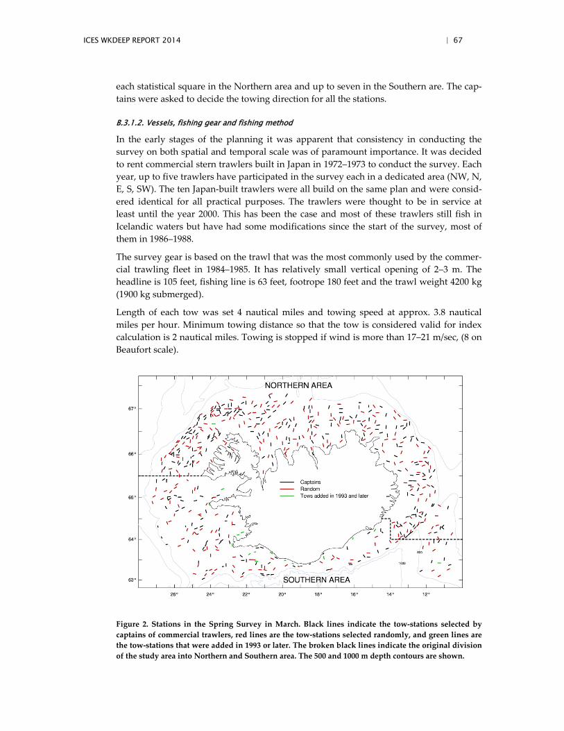
ICES WKDEEP REPORT 2014 | 67
each statistical square in the Northern area and up to seven in the Southern are. The cap-tains were asked to decide the towing direction for all the stations.
B.3.1.2. Vessels, fishing gear and fishing method
In the early stages of the planning it was apparent that consistency in conducting the survey on both spatial and temporal scale was of paramount importance. It was decided to rent commercial stern trawlers built in Japan in 1972–1973 to conduct the survey. Each year, up to five trawlers have participated in the survey each in a dedicated area (NW, N, E, S, SW). The ten Japan-built trawlers were all build on the same plan and were consid-ered identical for all practical purposes. The trawlers were thought to be in service at least until the year 2000. This has been the case and most of these trawlers still fish in Icelandic waters but have had some modifications since the start of the survey, most of them in 1986–1988.
The survey gear is based on the trawl that was the most commonly used by the commer-cial trawling fleet in 1984–1985. It has relatively small vertical opening of 2–3 m. The headline is 105 feet, fishing line is 63 feet, footrope 180 feet and the trawl weight 4200 kg (1900 kg submerged).
Length of each tow was set 4 nautical miles and towing speed at approx. 3.8 nautical miles per hour. Minimum towing distance so that the tow is considered valid for index calculation is 2 nautical miles. Towing is stopped if wind is more than 17–21 m/sec, (8 on Beaufort scale).
Figure 2. Stations in the Spring Survey in March. Black lines indicate the tow-stations selected by captains of commercial trawlers, red lines are the tow-stations selected randomly, and green lines are the tow-stations that were added in 1993 or later. The broken black lines indicate the original division of the study area into Northern and Southern area. The 500 and 1000 m depth contours are shown.
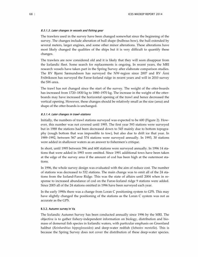
68 | ICES WKDEEP REPORT 2014
B.3.1.3. Later changes in vessels and fishing gear
The trawlers used in the survey have been changed somewhat since the beginning of the survey. The changes include alteration of hull shape (bulbous bow), the hull extended by several meters, larger engines, and some other minor alterations. These alterations have most likely changed the qualities of the ships but it is very difficult to quantify these changes.
The trawlers are now considered old and it is likely that they will soon disappear from the Icelandic fleet. Some search for replacements is ongoing. In recent years, the MRI research vessels have taken part in the Spring Survey after elaborate comparison studies. The RV Bjarni Sæmundsson has surveyed the NW-region since 2007 and RV Árni Friðriksson has surveyed the Faroe-Iceland ridge in recent years and will in 2010 survey the SW-area.
The trawl has not changed since the start of the survey. The weight of the otter-boards has increased from 1720–1830 kg to 1880–1970 kg. The increase in the weight of the otter-boards may have increased the horizontal opening of the trawl and hence decreased the vertical opening. However, these changes should be relatively small as the size (area) and shape of the otter-boards is unchanged.
B.3.1.4. Later changes in trawl-stations
Initially, the numbers of trawl stations surveyed was expected to be 600 (Figure 2). How-ever, this number was not covered until 1995. The first year 593 stations were surveyed but in 1988 the stations had been decreased down to 545 mainly due to bottom topogra-phy (rough bottom that was impossible to tow), but also due to drift ice that year. In 1989–1992, between 567 and 574 stations were surveyed annually. In 1993, 30 stations were added in shallower waters as an answer to fishermen’s critique.
In short, until 1995 between 596 and 600 stations were surveyed annually. In 1996 14 sta-tions that were added in 1993 were omitted. Since 1991 additional tows have been taken at the edge of the survey area if the amount of cod has been high at the outermost sta-tions.
In 1996, the whole survey design was evaluated with the aim of reduce cost. The number of stations was decreased to 532 stations. The main change was to omit all of the 24 sta-tions from the Iceland-Faroe Ridge. This was the state of affairs until 2004 when in re-sponse to increased abundance of cod on the Faroe-Iceland ridge 9 stations were added. Since 2005 all of the 24 stations omitted in 1996 have been surveyed each year.
In the early 1990s there was a change from Loran C positioning system to GPS. This may have slightly changed the positioning of the stations as the Loran C system was not as accurate as the GPS.
B.3.2. Autumn survey in Va
The Icelandic Autumn Survey has been conducted annually since 1996 by the MRI. The objective is to gather fishery-independent information on biology, distribution and bio-mass of demersal fish species in Icelandic waters, with particular emphasis on Greenland halibut (Reinhardtius hippoglossoides) and deep-water redfish (Sebastes mentella). This is because the Spring Survey does not cover the distribution of these deep-water species.
ICES WKDEEP REPORT 2014 | 69
Secondary aim of the survey is to have another fishery-independent estimate on abun-dance, biomass and biology of demersal species, such as cod (Gadus morhua), haddock (Melanogrammus aeglefinus) and golden redfish (Sebastes marinus), in order to improve the precision of stock assessment.
B.3.2.1. Timing, area covered and tow location
The Autumn Survey is conducted in October as it is considered the most a suitable month in relation to diurnal vertical migration, distribution and availability of Greenland halibut and deep-sea redfish. The research area is the Icelandic continental shelf and slopes within the Icelandic Exclusive Economic Zone to depths down to 1500 m. The research area is divided into a shallow-water area (0–400 m) and a deep-water area (400–1500 m). The shallow-water area is the same area covered in the Spring Survey. The deep-water area is directed at the distribution of Greenland halibut, mainly found at depths from 800–1400 m west, north and east of Iceland, and deep-water redfish, mainly found at 500–1200 m depths southeast, south and southwest of Iceland and on the Rey-kjanes Ridge.
B.3.2.2. Preparation and later alterations to the survey
Initially, a total of 430 stations were divided between the two areas. Of them, 150 stations were allocated to the shallow-water area and randomly selected from the Spring Survey station list. In the deep-water area, half of the 280 stations were randomly positioned in the area. The other half were randomly chosen from logbooks of the commercial bottom-trawl fleet fishing for Greenland halibut and deep-water redfish in 1991–1995. The loca-tions of those stations were, therefore, based on distribution and pre-estimated density of the species.
Because MRI was not able to finance a project in order of this magnitude, it was decided to focus the deep-water part of the survey on the Greenland halibut main distributional area. For this reason, important deep-water redfish areas south and west of Iceland were omitted. The number and location of stations in the shallow-water area were unchanged.
The number of stations in the deep-water area was therefore reduced to 150. A total of 100 stations were randomly positioned in the area. The remaining stations were located on important Greenland halibut fishing grounds west, north and east of Iceland and ran-domly selected from a logbook database of the bottom-trawl fleet fishing for Greenland halibut 1991–1995. The number of stations in each area was partly based on total com-mercial catch.
In 2000, with the arrival of a new research vessel, MRI was able finance the project ac-cording to the original plan. Stations were added to cover the distribution of deep-water redfish and the location of the stations selected in a similar manner as for Greenland hal-ibut. A total of 30 stations were randomly assigned to the distribution area of deep-water redfish and 30 stations were randomly assigned to the main deep-water redfish fishing grounds based on logbooks of the bottom-trawl fleet 1996–1999.
In addition, 14 stations were randomly added in the deep-water area in areas where great variation had been observed in 1996–1999. However, because of rough bottom which made it impossible to tow, five stations have been omitted. Finally, 12 stations were add-
70 | ICES WKDEEP REPORT 2014
ed in 1999 in the shallow-water area, making total stations in the shallow-water area 162. Total number of stations taken since 2000 has been around 381 (Figure 3).
The RV “Bjarni Sæmundsson” has been used in the shallow-water area from the begin-ning of the survey. For the deep-water area MRI rented one commercial trawler 1996–1999, but in 2000 the commercial trawler was replaced by the RV “Árni Friðriksson”.
Figure 3. Stations in the Autumn Groundfish Survey (AGS). RV “Bjarni Sæmundsson” takes stations in the shallow-water area (red lines) and RV “Árni Friðriksson” takes stations in the deep-water areas (green lines), the blue lines are stations added in 2000.
B.3.2.3. Fishing gear
Two types of the bottom survey trawl “Gulltoppur” are used for sampling: “Gulltoppur” is used in the shallow water and “Gulltoppur 66.6m” is used in deep waters. The trawls were common among the Icelandic bottom-trawl fleet in the mid-1990s and are well suit-ed for fisheries on cod, Greenland halibut and redfish.
“Gulltoppur”, the bottom trawl used in the shallow water, has a headline of 31.0 m, and the fishing line is 19.6 m. The deep-water trawl, “Gulltoppur 66.6m” has a headline of 35.6 m and the fishing line is 22.6 m.
The towing speed is 3.8 knots over the bottom. The trawling distance is 3.0 nautical miles calculated with GPS when the trawl touches the bottom until the hauling begins (i.e. ex-cluding setting and hauling of the trawl).
B.3.3. Data sampling
The data sampling in the spring and autumn surveys is quite similar. In short there is more emphasis on stomach content analysis in the Autumn Survey than the Spring Sur-
ICES WKDEEP REPORT 2014 | 71
vey. For ling, the sampling procedure is the same in both surveys except ling is weighed un-gutted and stomach content analysed in the autumn survey.
B.3.3.1. Length measurements and counting
All fish species are measured for length. For the majority of species including ling, total length is measured to the nearest cm from the tip of the snout to the tip of the longer lobe of the caudal fin. At each station, the general rule, which also applies to ling, is to meas-ure at least 4 times the length interval of a given species. Example: If the continuous length distribution of ling at a given station is between 15 and 45 cm, the length interval is 30 cm and the number of measurements needed is 120. If the catch of ling at this station exceeds 120 individuals, the rest is counted.
Care is taken to ensure that the length measurement sampling is random so that the fish measured reflect the length distribution of the haul in question.
B.3.3.2. Recording of weight, sex and maturity stages
Sex and maturity data has been sampled for ling from the start of both surveys. Ling is weighted as un-gutted in the Autumn Survey.
B.3.3.3. Otolith sampling
For ling a minimum of five otoliths in the spring and autumn surveys is collected and a maximum of 25. Otoliths are sampled at a four fish interval so that if in total 40 lings are caught in a single haul, 10 otoliths are sampled.
B.3.3.4. Stomach sampling and analysis
Stomach samples of ling are routinely sampled in the Autumn Survey.
B.3.3.5. Information on tow, gear and environmental factors
At each station/haul relevant information on the haul and environmental factors, are filled out by the captain and the first officer in cooperation with the cruise leader.
Tow information
General: Year, Station, Vessel registry no., Cruise ID, Day/month, Statist. Square, Sub-square, Tow number, Gear type no., Mesh size, Briddles length (m).
Start of haul: Pos. N, Pos. W, Time (hour:min), Tow direction in degrees, Bottom depth (m), Towing depth (m), Vert. opening (m), Horizontal opening (m).
End of haul: Pos. N, Pos. W, Time (hour:min), Warp length (fm), Bottom depth (m), Tow length (naut. miles), Tow time (min) , Tow speed (knots).
Environmental factors: Wind direction, Air temperature °C, Wind speed, Bottom tem-perature °C, Sea surface, Surface temperature °C, Towing depth temperature °C, Cloud cover, Air pressure, Drift ice.
B.3.2.4. Data processing
B.3.2.4.1. Abundance and biomass estimates at a given station
72 | ICES WKDEEP REPORT 2014
As described above the normal procedure is to measure at least 4 times the length inter-val of a given species. The number of fish caught of the length interval L1 to L2 is given by:
Where nmeasured is the number of fished measured and ncounted is the number of fish counted.
Biomass of a given species at a given station is calculated as:
Where Li is length and α and β are coefficients of the length–weight relationship.
B.3.2.4.2. Index calculation
For calculation of indices the Cochran method is used (Cochran, 1977). The survey area is split into subareas or strata and an index for each subarea is calculated as the mean num-ber in a standardized tow, divided by the area covered multiplied with the size of the subarea. The total index is then a summed up estimates from the subareas.
A ‘tow-mile’ is assumed to be 0.00918 square nautical mile. That is the width of the area covered is assumed to be 17 m (17/1852=0.00918). The following equations are a mathe-matical representation of the procedure used to calculate the indices:
Where iZ is the mean catch (number or biomass) in the i-th stratum, Zi is the total quanti-ty of the index (abundance or biomass) in the I-th stratum and Ni the total number of tows in the i-th stratum. The index (abundance or biomass) of a stratum (Ii) is:
And the sample variance in the i-th stratum:
where Ai is the size of the i-th stratum in square nautical miles (nm2) and Atow is the size of the area surveyed in a single tow in nm2.
The index in a given region:
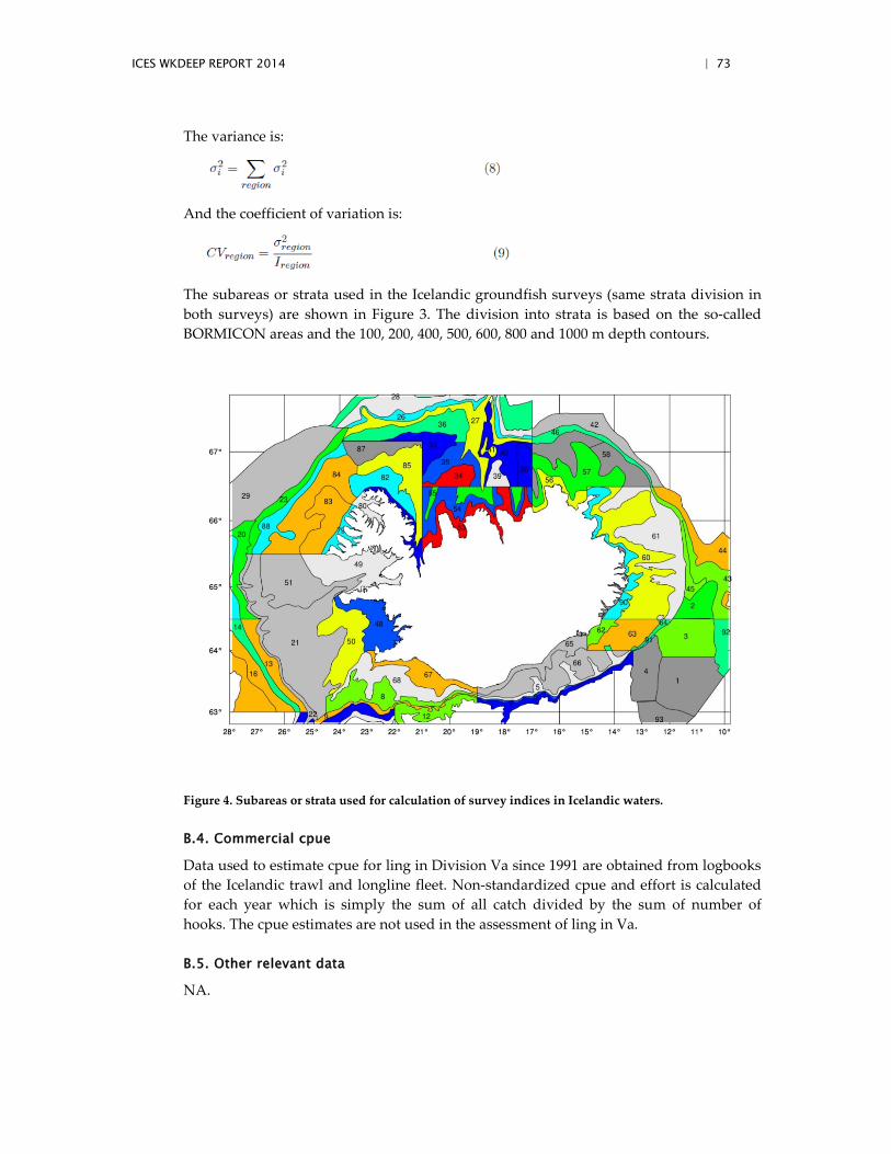
ICES WKDEEP REPORT 2014 | 73
The variance is:
And the coefficient of variation is:
The subareas or strata used in the Icelandic groundfish surveys (same strata division in both surveys) are shown in Figure 3. The division into strata is based on the so-called BORMICON areas and the 100, 200, 400, 500, 600, 800 and 1000 m depth contours.
Figure 4. Subareas or strata used for calculation of survey indices in Icelandic waters.
B.4. Commercial cpue
Data used to estimate cpue for ling in Division Va since 1991 are obtained from logbooks of the Icelandic trawl and longline fleet. Non-standardized cpue and effort is calculated for each year which is simply the sum of all catch divided by the sum of number of hooks. The cpue estimates are not used in the assessment of ling in Va.
B.5. Other relevant data
NA.
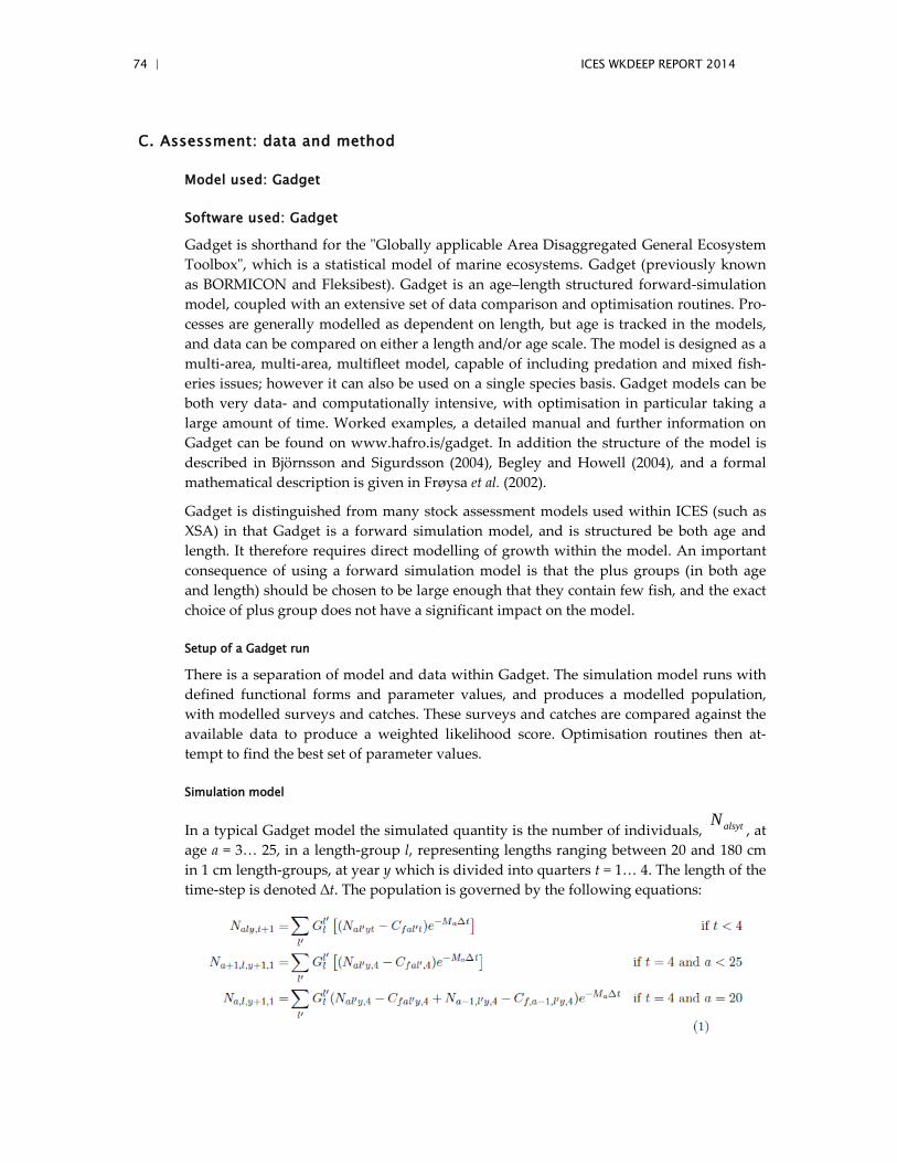
74 | ICES WKDEEP REPORT 2014
C. Assessment: data and method
Model used: Gadget
Software used: Gadget
Gadget is shorthand for the "Globally applicable Area Disaggregated General Ecosystem Toolbox", which is a statistical model of marine ecosystems. Gadget (previously known as BORMICON and Fleksibest). Gadget is an age–length structured forward-simulation model, coupled with an extensive set of data comparison and optimisation routines. Pro-cesses are generally modelled as dependent on length, but age is tracked in the models, and data can be compared on either a length and/or age scale. The model is designed as a multi-area, multi-area, multifleet model, capable of including predation and mixed fish-eries issues; however it can also be used on a single species basis. Gadget models can be both very data- and computationally intensive, with optimisation in particular taking a large amount of time. Worked examples, a detailed manual and further information on Gadget can be found on www.hafro.is/gadget. In addition the structure of the model is described in Björnsson and Sigurdsson (2004), Begley and Howell (2004), and a formal mathematical description is given in Frøysa et al. (2002).
Gadget is distinguished from many stock assessment models used within ICES (such as XSA) in that Gadget is a forward simulation model, and is structured be both age and length. It therefore requires direct modelling of growth within the model. An important consequence of using a forward simulation model is that the plus groups (in both age and length) should be chosen to be large enough that they contain few fish, and the exact choice of plus group does not have a significant impact on the model.
Setup of a Gadget run
There is a separation of model and data within Gadget. The simulation model runs with defined functional forms and parameter values, and produces a modelled population, with modelled surveys and catches. These surveys and catches are compared against the available data to produce a weighted likelihood score. Optimisation routines then at-tempt to find the best set of parameter values.
Simulation model
In a typical Gadget model the simulated quantity is the number of individuals, alsytN, at
age a = 3… 25, in a length-group l, representing lengths ranging between 20 and 180 cm in 1 cm length-groups, at year y which is divided into quarters t = 1… 4. The length of the time-step is denoted ∆t. The population is governed by the following equations:
ICES WKDEEP REPORT 2014 | 75
Where '
1lG is the proportion in length-group l that has grown l' - l length-groups in ∆t,
Cfalsyt denotes the catches by fleet f ∈{S, T, G, L}, S and C denote the spring survey, trawl, gillnet and longline fleets respectively (The survey fleet catches are given a nominal catch to allow for survey age and length distribution predictions.), Ma the natural mortality-at-age a (A short note on notation, here l is used interchangeably as either the length-group or the midpoint of the length interval for that particular length-group, depending on the context.).
Growth
Growth in length is modelled as a two-stage process, an average length update in ∆t and a growth dispersion around the mean update (Stefansson 2005). Average length update is modelled by calculating the mean growth for each length group for each time-step, using a parametric growth function. In the current model a simplified form of the von Bertan-lanffy function has been employed to calculate this mean length update.
where l∞ is the terminal length and k is the annual growth rate.
Then the length distributions are updated according to the calculated mean growth by allowing some portion of the fish to have no growth, a proportion to grow by one length group and a proportion two length groups etc. How these proportions are selected affects the spread of the length distributions but these two equations must be satisfied:
Here ∆l is the calculated mean growth and pil is the proportion of fish in length group l growing i length groups. Here the growth is dispersed according to a beta-binomial dis-tribution parametrised by the following equation:
Where α is subject to
where n denotes the maximum length group growth and (l'-l) the number of length-groups grown.
Recruitment and initial abundance
Gadget allows for a number of relationships between stock recruitment and the size of the spawning stock to be defined. However in this model the number of recruits each year, Ry is estimated directly from the data.
Recruitment enters to the population according to:
76 | ICES WKDEEP REPORT 2014
where t' denotes the recruitment time-step, pl is the proportion in length-group l that is recruited which is determined by a normal density with mean according to the growth
model and variance 2yσ
.When more data are available the number of recruits, Ry is esti-mated directly.
A simple formulation of initial abundance in numbers is used for each age group in length-group l
:
where υa is the initial number-at-age a in the initial year and ql the proportion at length-group l which is determined by a normal density with a mean according to the growth
model in use and variance 2aσ .
Fleet operations
Catches are simulated based on reported total landings and a length based suitability function for each of the fleets (commercial fleets and surveys). Total landings are as-sumed to be known and the total biomass is simply offset by the landed catch. The catch-es for length-group l, fleet f at year y and time-step t are calculated as
where Eft is the landed biomass at time t and Sf(l) is the suitability of length-group l by fleet f defined as:
The weight, Wsl, at length-group l is calculated according to the following stock compo-nent specific length - weight relationship:
Observation model
A significant advantage of using an age–length structured model is that the modelled output can be compared directly against a wide variety of different data sources. It is not necessary to convert length into age data before comparisons. Gadget can use various types of data that can be included in the objective function. Length distributions, age length keys, survey indices by length or age, cpue data, mean length and/or weight at age, tagging data and stomach content data can all be used.
Importantly this ability to handle length data directly means that the model can be used for stocks such as ling in Va where age data are sparse. Length data can be used directly for model comparison. The model is able to combine a wide selection of the available data by using a maximum likelihood approach to find the best fit to a weighted sum of the datasets.
ICES WKDEEP REPORT 2014 | 77
In Gadget, data are assimilated using a weighted log—likelihood function. Here three types of data enter the likelihood, length based survey indices, length distributions from survey and commercial fleets and age–length distribution from the survey and commer-cial fleets.
Survey indices
For each length range g the survey index is compared to the modelled abundance at year y and time-step t using:
(eq 1)
Where
Fleet data
Length distributions are compared to predictions using
(eq 2)
where f denotes the fleet where data were sampled from and
i.e. the observed and modelled proportions in length-group l respectively at year y and time-step t. Similarly age - length data are compared using 1 cm length groups:
(eq 3)
Iterative re-weighting
The total objective function used the modelling process combines equations eq 1 to eq 3 using the following formula:
78 | ICES WKDEEP REPORT 2014
where f = S, T, G, L or C denotes the spring survey, trawl, gillnet and longline fleets re-spectively (See subsection and w's are the weights assigned to each likelihood compo-nents.
The weights, wi, are necessary for several reasons. First of all it is used to prevent some components from dominating the likelihood function. Another would be to reduce the effect of low quality data. It can be used as an a priori estimates of the variance in each subset of the data.
Assigning likelihood weights is not a trivial matter, has in the past been the most time consuming part of a Gadget model. Commonly this has been done using some form of 'expert judgement'. General heuristics have recently been developed to estimate these weights objectively. Here the iterative re--weighting heuristic introduced by Stefansson (2003), and subsequently implemented in Taylor (2007}, is used.
The general idea behind the iterative re-weighing is to assign the inverse variance of the fitted residuals as component weights. The variances, and hence the final weights, are calculated according the following algorithm:
1. Calculate the initial sums of squares (SS) given the initial parametrization for all likelihood components. Assign the inverse SS as the initial weight for all likeli-hood components.
2. For each likelihood component, do an optimization run with the initial SS for that component set to 10000. Then estimate the residual variance using the resulting
SS of that component divided by the degrees of freedom (df*), i.e. *ˆ 2
dfSS
=σ.
3. After the optimization set the final weight for that all components as the inverse
of the estimated variance from the step above (weight =1/2σ̂ ).
The number of non-zero data-points (df*) is used as a proxy for the degrees of freedom. While this may be a satisfactory proxy for larger datasets it could be a gross overestimate of the degrees of freedom for smaller datasets. In particular, if the survey indices are weighed on their own while the yearly recruitment is estimated they could be over-fitted. In general, problem such as these can be solved with component grouping that is in step 2 the likelihood components that should behave similarly, such as survey indices repre-senting similar age ranges, should be heavily weighted and optimized together. In the ling model this kind of grouping is used.
Optimisation
The model has three alternative optimising algorithms linked to it, a wide area search simulated annealing (Corana et al., 1987), a local search Hooke and Jeeves algorithm (Hooke & Jeeves 1961) and finally one based on the Boyden-Fletcher-Goldfarb-Shanno algorithm hereafter termed BFGS.
The simulated annealing and Hooke-Jeeves algorithms are not gradient based, and there is therefore no requirement on the likelihood surface being smooth. Consequently neither of the two algorithms returns estimates of the Hessian matrix. Simulated annealing is more robust than Hooke and Jeeves and can find a global optima where there are multi-
ICES WKDEEP REPORT 2014 | 79
ple optima but needs about 2-3 times the order of magnitude number of iterations than the Hooke and Jeeves algorithm.
BFGS is a quasi-Newton optimisation method that uses information about the gradient of the function at the current point to calculate the best direction to look for a better point. Using this information the BFGS algorithm can iteratively calculate a better approxima-tion to the inverse Hessian matrix. In comparison to the two other algorithms imple-mented in Gadget, BFGS is very local search compared to simulated annealing and more computationally intensive than the Hooke and Jeeves. However the gradient search in BFGS is more accurate than the stepwise search of Hooke and Jeeves and may therefore give a more accurate estimation of the optimum. The BFGS algorithm used in Gadget is derived from that presented by Bertsekas (1999).
The model is able to use ll three algorithms in a single optimisation run, attempting to utilise the strengths of all. Simulated annealing is used first to attempt to reach the gen-eral area of a solution, followed by Hooke and Jeeves to rapidly home in on the local solution and finally BFGS is used for fine-tuning the optimisation. This procedure is re-peated several times to attempt to avoid converging to a local optimum.
The total objective function to be minimised is a weighted sum of the different compo-nents. The estimation can be difficult because of some or groups of parameters are corre-lated and therefore the possibility of multiple optima cannot be excluded. The optimisation was started with simulated annealing to make the results less sensitive to the initial (starting) values and then the optimisation was changed to Hooke and Jeeves when the 'optimum' was approached and then finally the BFGS was run in the end.
Model settings
Population is defined by 1 cm length groups, from 20–180 cm and the year is divided into four quarters. The age range is 2 to 20 years, with the oldest age treated as a plus group. Recruitment happens in the first and was set at age 2. The length-at-recruitment is esti-mated and mean growth is assumed to follow the von Bertalanffy growth function esti-mated by the model.
Weight Length relationship is obtained from spring survey data.
Natural mortality was assumed to be 0.15 year-1.
The commercial landings are modelled as three fleets, longline, trawl and gillnet, starting in 1982 with a selection patterns described by a logistic function and the total catch in tonnes specified for each quarter. The survey (1985 onwards), on the other hand is mod-elled as one fleet with constant effort and a nonparametric selection pattern that is esti-mated for each length group (one 10 cm length group).
Data used for the assessment are described below
Length disaggregated survey indices (10 cm increments, except the smallest 20–50cm and the largest 90–180cm) from the Icelandic groundfish survey in March 1985–onwards.
Length distribution from the Icelandic commercial catch since 1982. The sampling effort was though relatively limited until the 1990s.
Landings data divided into 4 month periods per year (quarters).

80 | ICES WKDEEP REPORT 2014
Age–length data from the survey and from the commercial fleets
DESCRIPTION PERIOD BY QUARTER AREA LIKELIHOOD
COMPONENT
Length distribution of landings
Longline, trawl, gillnet
1982+ All Iceland ldist.catch
Length distribution of Icelandic GFS
1985+ 1st quarter Iceland ldist.survey
Abundace index of Icelandic GFS of 20–49 cm individuals
1985+ 1st quarter Iceland si2049
Abundace index of Icelandic GFS of 50-69 cm individuals
1985+ 1st quarter Iceland Si5069
Abundace index of Icelandic GFS of 70–180 cm individuals
1985+ 1st quarter Iceland Si70180
Age–length key of the landings See stock section
All Iceland alkeys.longline, alkeys.trawl, alkeys.gillnet
Age–length key of the Icelandic GFS
See stock section
1st quarter Iceland alkeys.survey
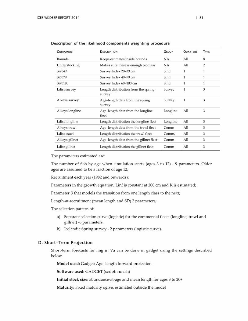
ICES WKDEEP REPORT 2014 | 81
Description of the likelihood components weighting procedure
COMPONENT DESCRIPTION GROUP QUARTERS TYPE
Bounds Keeps estimates inside bounds NA All 8
Understocking Makes sure there is enough biomass NA All 2
Si2049 Survey Index 20–39 cm Sind 1 1
Si5079 Survey Index 40–59 cm Sind 1 1
Si70180 Survey Index 60–100 cm Sind 1 1
Ldist.survey Length distribution from the spring survey
Survey 1 3
Alkeys.survey Age–length data from the spring survey
Survey 1 3
Alkeys.longline Age–length data from the longline fleet
Longline All 3
Ldist.longline Length distribution the longline fleet Longline All 3
Alkeys.trawl Age–length data from the trawl fleet Comm All 3
Ldist.trawl Length distribution the trawl fleet Comm. All 3
Alkeys.gillnet Age–length data from the gillnet fleet Comm All 3
Ldist.gillnet Length distribution the gillnet fleet Comm All 3
The parameters estimated are:
The number of fish by age when simulation starts (ages 3 to 12) - 9 parameters. Older ages are assumed to be a fraction of age 12;
Recruitment each year (1982 and onwards);
Parameters in the growth equation; Linf is constant at 200 cm and K is estimated;
Parameter β that models the transition from one length class to the next;
Length-at-recruitment (mean length and SD) 2 parameters;
The selection pattern of:
a) Separate selection curve (logistic) for the commercial fleets (longline, trawl and gillnet) -6 parameters.
b) Icelandic Spring survey - 2 parameters (logistic curve).
D. Short-Term Projection
Short-term forecasts for ling in Va can be done in gadget using the settings described below.
Model used: Gadget: Age–length forward projection
Software used: GADGET (script: run.sh)
Initial stock size: abundance-at-age and mean length for ages 3 to 20+
Maturity: Fixed maturity ogive, estimated outside the model
82 | ICES WKDEEP REPORT 2014
F and M before spawning: NA
Weight-at-age in the stock: modelled in GADGET with VB parameters and length–weight relationship that is estimated outside the model.
Weight-at-age in the catch: modelled in GADGET with VB parameters and length–weight relationship
Exploitation pattern: Landings: logistic selection parameters estimated by GADGET. Fleet proportions set as last three years average
Intermediate year assumptions: Catch in first quarter known, catches in quarters 2, 3 and 4 assumed to be equal to last years.
Stock recruitment model used: Mean of last three years. As recruitment is estimated at age three in the assessment but ling does not appear in the catches until the age of 5 the recruitment assumptions are not important.
Procedures used for splitting projected catches: driven by selection functions and provide by GADGET. Fleet proportions set as last three years average
E. Medium-Term Projections
Short-term forecasts for ling in Va can be done in gadget using the settings described below.
Model used: Gadget: Age–length forward projection
Software used: GADGET (script: run.sh)
Initial stock size: abundance-at-age and mean length for ages 3 to 20+
Maturity: Fixed maturity ogive, estimated outside the model
F and M before spawning: NA
Weight-at-age in the stock: modelled in GADGET with VB parameters and length–weight relationship that is estimated outside the model.
Weight-at-age in the catch: modelled in GADGET with VB parameters and length–weight relationship
Exploitation pattern: Landings: logistic selection parameters estimated by GADGET. Fleet proportions set as last three years average
Intermediate year assumptions: Catch in first quarter known, catches in quarters 2, 3 and 4 assumed to be equal to last years.
Stock recruitment model used: Mean of last three years.
Procedures used for splitting projected catches: driven by selection functions and provide by GADGET. Fleet proportions set as last three years average
Uncertainty models used:
To estimate the uncertainty in the model parameters and derived quantities a specialised bootstrap for disparate datasets is used. The approach is based on spatial subdivisions
ICES WKDEEP REPORT 2014 | 83
that can be considered to be i.i.d. Refer to Elvarsson (2014) for further details. The boot-strapping approach consists of the following:
• The base data are stored in a standardized database:
o Time aggregation: 3 months
o Spatial aggregation: subdivision
o Further dis-aggregation is based on a range of categories including fish-ing gear, fishing vessel class, sampling type (e.g. harbour, sea and sur-vey).
• To bootstrap the data, the list of subdivisions, depicted in figure E1, required for the model is sampled (with replacement) and stored. For a multi--area model one would conduct the re-sampling of subdivisions within each area of the model.
• The list of resampled subdivisions is then used to extract data (with replacement so the same dataset may be repeated several times in a given bootstrap sample).
• For a single bootstrap Gadget model, the same list of resampled subdivisions is used to extract each likelihood dataset i.e. length distributions, survey indices and age--length frequencies are extracted from the same spatial definition.
• A Gadget model is fitted to the extracted bootstrap dataset using the estimation procedure described above.
• The re-sampling process is repeated until the desired number of bootstrap sam-ples are extracted, which in this case the total sample size is 100.
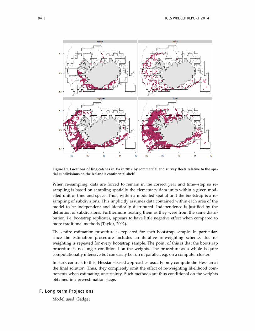
84 | ICES WKDEEP REPORT 2014
Figure E1. Locations of ling catches in Va in 2012 by commercial and survey fleets relative to the spa-tial subdivisions on the Icelandic continental shelf.
When re-sampling, data are forced to remain in the correct year and time--step so re-sampling is based on sampling spatially the elementary data units within a given mod-elled unit of time and space. Thus, within a modelled spatial unit the bootstrap is a re-sampling of subdivisions. This implicitly assumes data contained within each area of the model to be independent and identically distributed. Independence is justified by the definition of subdivisions. Furthermore treating them as they were from the same distri-bution, i.e. bootstrap replicates, appears to have little negative effect when compared to more traditional methods (Taylor, 2002).
The entire estimation procedure is repeated for each bootstrap sample. In particular, since the estimation procedure includes an iterative re-weighting scheme, this re-weighting is repeated for every bootstrap sample. The point of this is that the bootstrap procedure is no longer conditional on the weights. The procedure as a whole is quite computationally intensive but can easily be run in parallel, e.g. on a computer cluster.
In stark contrast to this, Hessian--based approaches usually only compute the Hessian at the final solution. Thus, they completely omit the effect of re-weighting likelihood com-ponents when estimating uncertainty. Such methods are thus conditional on the weights obtained in a pre-estimation stage.
F. Long term Projections
Model used: Gadget
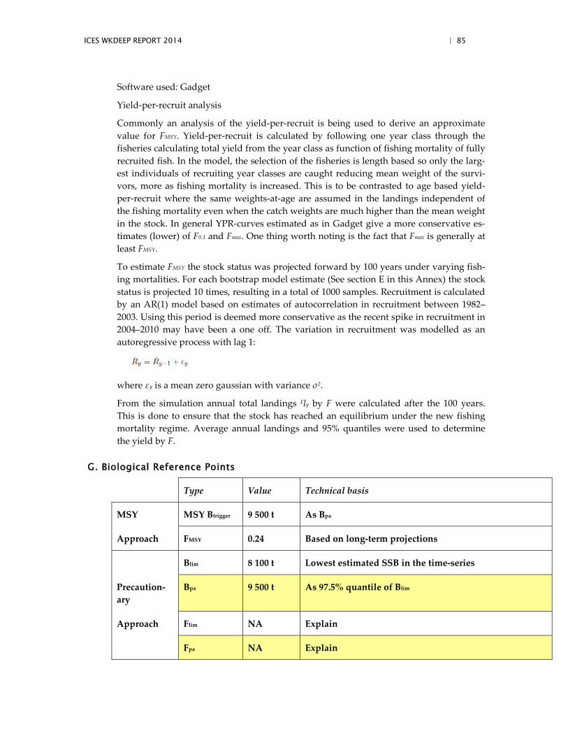
ICES WKDEEP REPORT 2014 | 85
Software used: Gadget
Yield-per-recruit analysis
Commonly an analysis of the yield-per-recruit is being used to derive an approximate value for FMSY. Yield-per-recruit is calculated by following one year class through the fisheries calculating total yield from the year class as function of fishing mortality of fully recruited fish. In the model, the selection of the fisheries is length based so only the larg-est individuals of recruiting year classes are caught reducing mean weight of the survi-vors, more as fishing mortality is increased. This is to be contrasted to age based yield-per-recruit where the same weights-at-age are assumed in the landings independent of the fishing mortality even when the catch weights are much higher than the mean weight in the stock. In general YPR-curves estimated as in Gadget give a more conservative es-timates (lower) of F0.1 and Fmax. One thing worth noting is the fact that Fmax is generally at least FMSY.
To estimate FMSY the stock status was projected forward by 100 years under varying fish-ing mortalities. For each bootstrap model estimate (See section E in this Annex) the stock status is projected 10 times, resulting in a total of 1000 samples. Recruitment is calculated by an AR(1) model based on estimates of autocorrelation in recruitment between 1982–2003. Using this period is deemed more conservative as the recent spike in recruitment in 2004–2010 may have been a one off. The variation in recruitment was modelled as an autoregressive process with lag 1:
where εy is a mean zero gaussian with variance σ2.
From the simulation annual total landings Fly by F were calculated after the 100 years. This is done to ensure that the stock has reached an equilibrium under the new fishing mortality regime. Average annual landings and 95% quantiles were used to determine the yield by F.
G. Biological Reference Points
Type Value Technical basis
MSY MSY Btrigger 9 500 t As Bpa
Approach FMSY 0.24 Based on long-term projections
Blim 8 100 t Lowest estimated SSB in the time-series
Precaution-ary
Bpa 9 500 t As 97.5% quantile of Blim
Approach Flim NA Explain
Fpa NA Explain
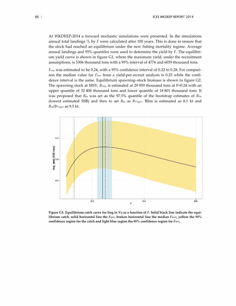
86 | ICES WKDEEP REPORT 2014
At WKDEEP-2014 a forward stochastic simulations were presented. In the simulations annual total landings Fly by F were calculated after 100 years. This is done to ensure that the stock had reached an equilibrium under the new fishing mortality regime. Average annual landings and 95% quantiles were used to determine the yield by F. The equilibri-um yield curve is shown in figure G1, where the maximum yield, under the recruitment assumptions, is 5306 thousand tons with a 95% interval of 4776 and 6059 thousand tons.
Fmsy was estimated to be 0.24, with a 95% confidence interval of 0.22 to 0.28. For compari-son the median value for Fmax from a yield-per-recruit analysis is 0.25 while the confi-dence interval is the same. Equilibrium spawning–stock biomass is shown in figure G2. The spawning stock at MSY, Bmsy, is estimated at 29 959 thousand tons at F=0.24 with an upper quantile of 32 408 thousand tons and lower quantile of 18 801 thousand tons. It was proposed that Bpa was set as the 97.5% quantile of the bootstrap estimates of Blim (lowest estimated SSB) and then to set Bpa as BTrigger. Blim is estimated as 8.1 kt and Bpa/BTrigger as 9.5 kt.
Figure G1. Equilibrium catch curve for ling in Va as a function of F. Solid black line indicate the equi-librium catch, solid horizontal line the FMSY, broken horizontal line the median FMAX, yellow the 95% confidence region for the catch and light blue region the 95% confidence region for FMSY.
ICES WKDEEP REPORT 2014 | 87
Figure G2. Equilibrium spawning-stock biomass as a function of F. Solid black line indicate the equi-librium biomass, solid horizontal line the FMSY, broken horizontal line the median FMAX, yellow the 95% confidence region for the biomass and light blue region the 95% confidence region for FMSY. Red area is BPA (BTrigger)
H. Other Issues
H.1. Historical overview of previous assessment methods
Before 2007 ling in the NE-Atlantic was assessed as a single management unit.
Between 2007 to 2012 ling in Va was assessed based on trends in survey indices from the Icelandic spring and autumn survey. Supplementary information included relevant in-formation from the fishery such as length distributions, maturity data, effort, cpue and analysis of changes in spatial and temporal distribution.
In 2012 the stock was assessed as a category 3 stock in the ICES-DLS framework and the basis for the ICES advice was
IndexYieldFproxy =
The rationale for the advice was: For this stock the Fproxy of 1.5 is applied as a factor of the average of the most recent survey biomass estimates (average of 2011 and 2012), resulting in catch advice of no more than 12 000 t. i.e. to base the catches in 2013 and 2014 on 1.5 the survey biomass in 2012.
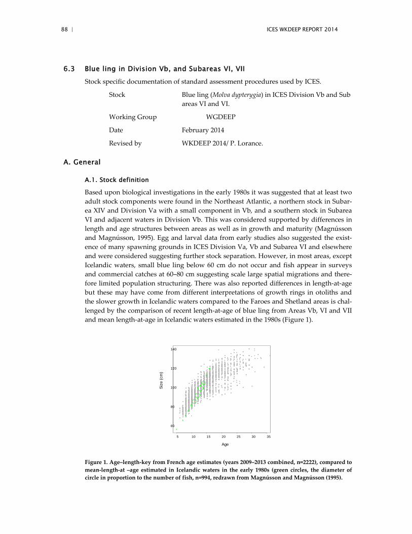
88 | ICES WKDEEP REPORT 2014
6.3 Blue ling in Division Vb, and Subareas VI, VII
Stock specific documentation of standard assessment procedures used by ICES.
Stock Blue ling (Molva dypterygia) in ICES Division Vb and Sub areas VI and VI.
Working Group WGDEEP
Date February 2014
Revised by WKDEEP 2014/ P. Lorance.
A. General
A.1. Stock definition
Based upon biological investigations in the early 1980s it was suggested that at least two adult stock components were found in the Northeast Atlantic, a northern stock in Subar-ea XIV and Division Va with a small component in Vb, and a southern stock in Subarea VI and adjacent waters in Division Vb. This was considered supported by differences in length and age structures between areas as well as in growth and maturity (Magnússon and Magnússon, 1995). Egg and larval data from early studies also suggested the exist-ence of many spawning grounds in ICES Division Va, Vb and Subarea VI and elsewhere and were considered suggesting further stock separation. However, in most areas, except Icelandic waters, small blue ling below 60 cm do not occur and fish appear in surveys and commercial catches at 60–80 cm suggesting scale large spatial migrations and there-fore limited population structuring. There was also reported differences in length-at-age but these may have come from different interpretations of growth rings in otoliths and the slower growth in Icelandic waters compared to the Faroes and Shetland areas is chal-lenged by the comparison of recent length-at-age of blue ling from Areas Vb, VI and VII and mean length-at-age in Icelandic waters estimated in the 1980s (Figure 1).
Figure 1. Age–length-key from French age estimates (years 2009–2013 combined, n=2222), compared to mean-length-at –age estimated in Icelandic waters in the early 1980s (green circles, the diameter of circle in proportion to the number of fish, n=994, redrawn from Magnússon and Magnússon (1995).
5 10 15 20 25 30 35
60
80
100
120
140
Age
Size
(cm
)
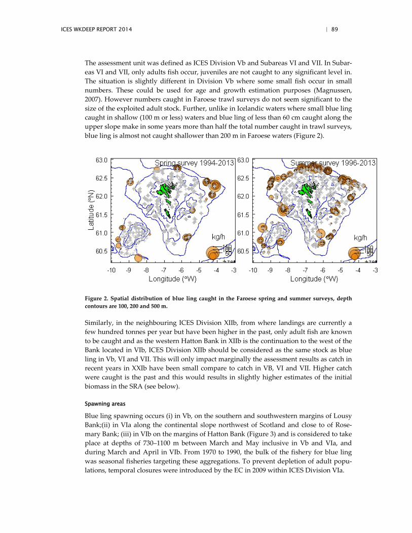
ICES WKDEEP REPORT 2014 | 89
The assessment unit was defined as ICES Division Vb and Subareas VI and VII. In Subar-eas VI and VII, only adults fish occur, juveniles are not caught to any significant level in. The situation is slightly different in Division Vb where some small fish occur in small numbers. These could be used for age and growth estimation purposes (Magnussen, 2007). However numbers caught in Faroese trawl surveys do not seem significant to the size of the exploited adult stock. Further, unlike in Icelandic waters where small blue ling caught in shallow (100 m or less) waters and blue ling of less than 60 cm caught along the upper slope make in some years more than half the total number caught in trawl surveys, blue ling is almost not caught shallower than 200 m in Faroese waters (Figure 2).
Figure 2. Spatial distribution of blue ling caught in the Faroese spring and summer surveys, depth contours are 100, 200 and 500 m.
Similarly, in the neighbouring ICES Division XIIb, from where landings are currently a few hundred tonnes per year but have been higher in the past, only adult fish are known to be caught and as the western Hatton Bank in XIIb is the continuation to the west of the Bank located in VIb, ICES Division XIIb should be considered as the same stock as blue ling in Vb, VI and VII. This will only impact marginally the assessment results as catch in recent years in XXIb have been small compare to catch in VB, VI and VII. Higher catch were caught is the past and this would results in slightly higher estimates of the initial biomass in the SRA (see below).
Spawning areas
Blue ling spawning occurs (i) in Vb, on the southern and southwestern margins of Lousy Bank;(ii) in VIa along the continental slope northwest of Scotland and close to of Rose-mary Bank; (iii) in VIb on the margins of Hatton Bank (Figure 3) and is considered to take place at depths of 730–1100 m between March and May inclusive in Vb and VIa, and during March and April in VIb. From 1970 to 1990, the bulk of the fishery for blue ling was seasonal fisheries targeting these aggregations. To prevent depletion of adult popu-lations, temporal closures were introduced by the EC in 2009 within ICES Division VIa.
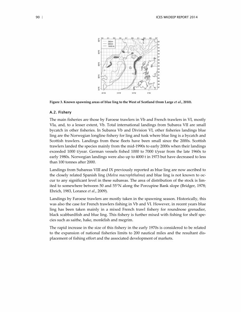
90 | ICES WKDEEP REPORT 2014
Figure 3. Known spawning areas of blue ling to the West of Scotland (from Large et al., 2010).
A.2. Fishery
The main fisheries are those by Faroese trawlers in Vb and French trawlers in VI, mostly VIa, and, to a lesser extent, Vb. Total international landings from Subarea VII are small bycatch in other fisheries. In Subarea Vb and Division VI, other fisheries landings blue ling are the Norwegian longline fishery for ling and tusk where blue ling is a bycatch and Scottish trawlers. Landings from these fleets have been small since the 2000s. Scottish trawlers landed the species mainly from the mid-1990s to early 2000s when their landings exceeded 1000 t/year. German vessels fished 1000 to 7000 t/year from the late 1960s to early 1980s. Norwegian landings were also up to 4000 t in 1973 but have decreased to less than 100 tonnes after 2000.
Landings from Subareas VIII and IX previously reported as blue ling are now ascribed to the closely related Spanish ling (Molva macrophthalma) and blue ling is not known to oc-cur to any significant level in these subareas. The area of distribution of the stock is lim-ited to somewhere between 50 and 55°N along the Porcupine Bank slope (Bridger, 1978; Ehrich, 1983, Lorance et al., 2009).
Landings by Faroese trawlers are mostly taken in the spawning season. Historically, this was also the case for French trawlers fishing in Vb and VI. However, in recent years blue ling has been taken mainly in a mixed French trawl fishery for roundnose grenadier, black scabbardfish and blue ling. This fishery is further mixed with fishing for shelf spe-cies such as saithe, hake, monkfish and megrim.
The rapid increase in the size of this fishery in the early 1970s is considered to be related to the expansion of national fisheries limits to 200 nautical miles and the resultant dis-placement of fishing effort and the associated development of markets.
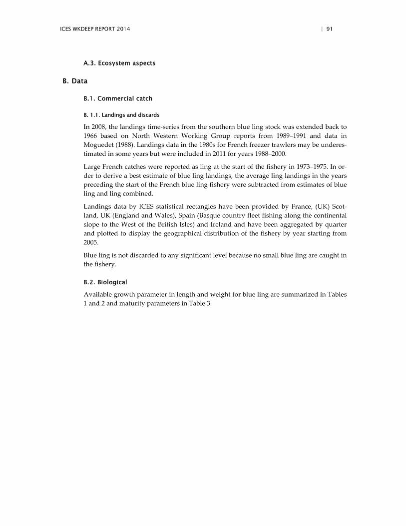
ICES WKDEEP REPORT 2014 | 91
A.3. Ecosystem aspects
B. Data
B.1. Commercial catch
B. 1.1. Landings and discards
In 2008, the landings time-series from the southern blue ling stock was extended back to 1966 based on North Western Working Group reports from 1989–1991 and data in Moguedet (1988). Landings data in the 1980s for French freezer trawlers may be underes-timated in some years but were included in 2011 for years 1988–2000.
Large French catches were reported as ling at the start of the fishery in 1973–1975. In or-der to derive a best estimate of blue ling landings, the average ling landings in the years preceding the start of the French blue ling fishery were subtracted from estimates of blue ling and ling combined.
Landings data by ICES statistical rectangles have been provided by France, (UK) Scot-land, UK (England and Wales), Spain (Basque country fleet fishing along the continental slope to the West of the British Isles) and Ireland and have been aggregated by quarter and plotted to display the geographical distribution of the fishery by year starting from 2005.
Blue ling is not discarded to any significant level because no small blue ling are caught in the fishery.
B.2. Biological
Available growth parameter in length and weight for blue ling are summarized in Tables 1 and 2 and maturity parameters in Table 3.
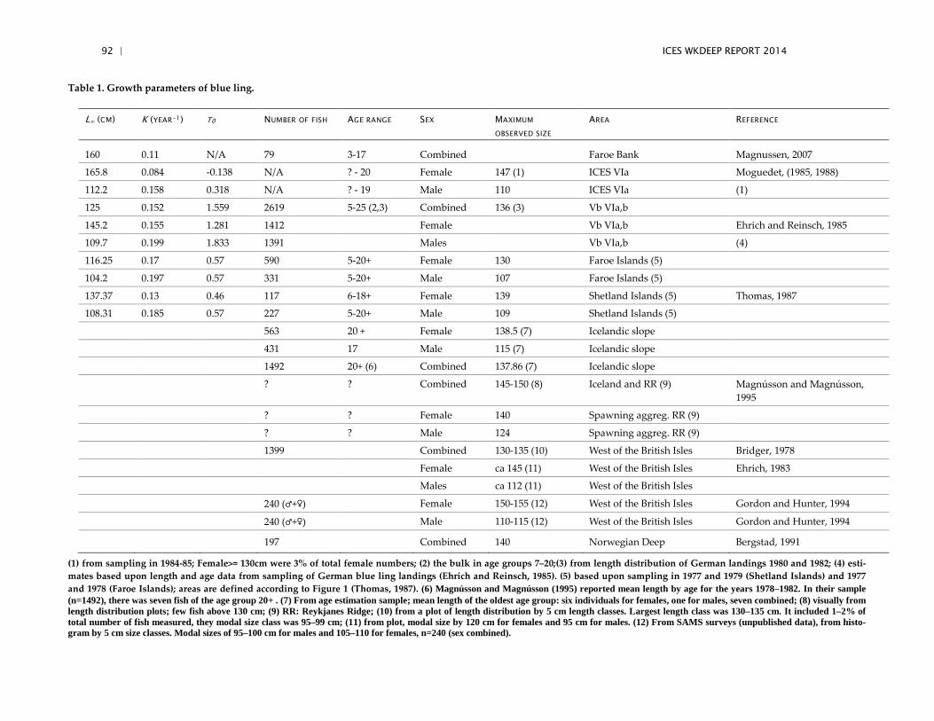
92 | ICES WKDEEP REPORT 2014
Table 1. Growth parameters of blue ling.
L∞ (CM) K (YEAR-1) T0 NUMBER OF FISH AGE RANGE SEX MAXIMUM OBSERVED SIZE
AREA REFERENCE
160 0.11 N/A 79 3-17 Combined Faroe Bank Magnussen, 2007
165.8 0.084 -0.138 N/A ? - 20 Female 147 (1) ICES VIa Moguedet, (1985, 1988)
112.2 0.158 0.318 N/A ? - 19 Male 110 ICES VIa (1)
125 0.152 1.559 2619 5-25 (2,3) Combined 136 (3) Vb VIa,b
145.2 0.155 1.281 1412 Female Vb VIa,b Ehrich and Reinsch, 1985
109.7 0.199 1.833 1391 Males Vb VIa,b (4)
116.25 0.17 0.57 590 5-20+ Female 130 Faroe Islands (5)
104.2 0.197 0.57 331 5-20+ Male 107 Faroe Islands (5)
137.37 0.13 0.46 117 6-18+ Female 139 Shetland Islands (5) Thomas, 1987
108.31 0.185 0.57 227 5-20+ Male 109 Shetland Islands (5)
563 20 + Female 138.5 (7) Icelandic slope
431 17 Male 115 (7) Icelandic slope
1492 20+ (6) Combined 137.86 (7) Icelandic slope
? ? Combined 145-150 (8) Iceland and RR (9) Magnússon and Magnússon, 1995
? ? Female 140 Spawning aggreg. RR (9)
? ? Male 124 Spawning aggreg. RR (9)
1399 Combined 130-135 (10) West of the British Isles Bridger, 1978
Female ca 145 (11) West of the British Isles Ehrich, 1983
Males ca 112 (11) West of the British Isles
240 (♂+♀) Female 150-155 (12) West of the British Isles Gordon and Hunter, 1994
240 (♂+♀) Male 110-115 (12) West of the British Isles Gordon and Hunter, 1994
197 Combined 140 Norwegian Deep Bergstad, 1991
(1) from sampling in 1984-85; Female>= 130cm were 3% of total female numbers; (2) the bulk in age groups 7–20;(3) from length distribution of German landings 1980 and 1982; (4) esti-mates based upon length and age data from sampling of German blue ling landings (Ehrich and Reinsch, 1985). (5) based upon sampling in 1977 and 1979 (Shetland Islands) and 1977 and 1978 (Faroe Islands); areas are defined according to Figure 1 (Thomas, 1987). (6) Magnússon and Magnússon (1995) reported mean length by age for the years 1978–1982. In their sample (n=1492), there was seven fish of the age group 20+ . (7) From age estimation sample; mean length of the oldest age group: six individuals for females, one for males, seven combined; (8) visually from length distribution plots; few fish above 130 cm; (9) RR: Reykjanes Ridge; (10) from a plot of length distribution by 5 cm length classes. Largest length class was 130–135 cm. It included 1–2% of total number of fish measured, they modal size class was 95–99 cm; (11) from plot, modal size by 120 cm for females and 95 cm for males. (12) From SAMS surveys (unpublished data), from histo-gram by 5 cm size classes. Modal sizes of 95–100 cm for males and 105–110 for females, n=240 (sex combined).
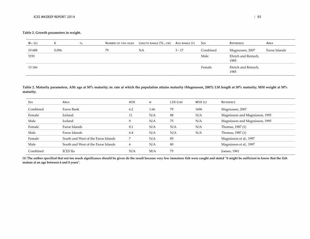
ICES WKDEEP REPORT 2014 | 93
Table 2. Growth parameters in weight.
W∞ (G) K T0 NUMBER OF FISH AGED LENGTH RANGE (TL, CM) AGE RANGE (Y) SEX REFERENCE AREA
19 688 0.094 79 NA 3 - 17 Combined Magnussen, 2007 Faroe Islands
5191 Male Ehrich and Reinsch, 1985
13 166 Female Ehrich and Reinsch, 1985
Table 2. Maturity parameters, A50: age at 50% maturity; m: rate at which the population attains maturity (Magnussen, 2007); L50 length at 50% maturity; M50 weight at 50% maturity.
SEX AREA A50 M L50 (CM) M50 (G) REFERENCE
Combined Faroe Bank 6.2 1.66 79 1696 Magnussen, 2007
Female Iceland 11 N/A 88 N/A Magnússon and Magnússon, 1995
Male Iceland 9 N/A 75 N/A Magnússon and Magnússon, 1995
Female Faroe Islands 8.1 N/A N/A N/A Thomas, 1987 (1)
Male Faroe Islands 6.4 N/A N/A N/A Thomas, 1987 (1)
Female South and West of the Faroe Islands 7 N/A 85 Magnússon et al., 1997
Male South and West of the Faroe Islands 6 N/A 80 Magnússon et al., 1997
Combined ICES IIa N/A M/A 75 Joenes, 1961
(1) The author specified that not too much significance should be given do the result because very few immature fish were caught and stated "it might be sufficient to know that the fish mature at an age between 6 and 8 years".
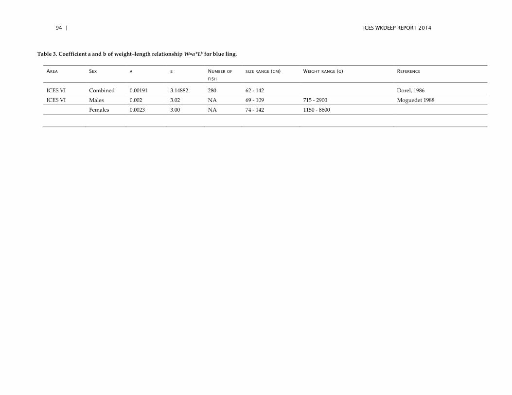
94 | ICES WKDEEP REPORT 2014
Table 3. Coefficient a and b of weight–length relationship W=a*Lb for blue ling.
AREA SEX A B NUMBER OF
FISH SIZE RANGE (CM) WEIGHT RANGE (G) REFERENCE
ICES VI Combined 0.00191 3.14882 280 62 - 142 Dorel, 1986
ICES VI Males 0.002 3.02 NA 69 - 109 715 - 2900 Moguedet 1988
Females 0.0023 3.00 NA 74 - 142 1150 - 8600
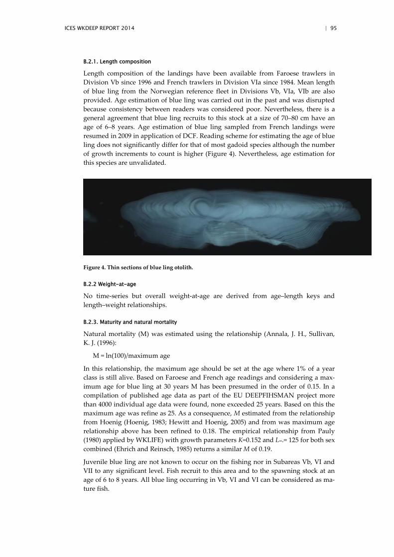
ICES WKDEEP REPORT 2014 | 95
B.2.1. Length composition
Length composition of the landings have been available from Faroese trawlers in Division Vb since 1996 and French trawlers in Division VIa since 1984. Mean length of blue ling from the Norwegian reference fleet in Divisions Vb, VIa, VIb are also provided. Age estimation of blue ling was carried out in the past and was disrupted because consistency between readers was considered poor. Nevertheless, there is a general agreement that blue ling recruits to this stock at a size of 70–80 cm have an age of 6–8 years. Age estimation of blue ling sampled from French landings were resumed in 2009 in application of DCF. Reading scheme for estimating the age of blue ling does not significantly differ for that of most gadoid species although the number of growth increments to count is higher (Figure 4). Nevertheless, age estimation for this species are unvalidated.
Figure 4. Thin sections of blue ling otolith.
B.2.2 Weight-at-age
No time-series but overall weight-at-age are derived from age–length keys and length–weight relationships.
B.2.3. Maturity and natural mortality
Natural mortality (M) was estimated using the relationship (Annala, J. H., Sullivan, K. J. (1996):
M = ln(100)/maximum age
In this relationship, the maximum age should be set at the age where 1% of a year class is still alive. Based on Faroese and French age readings and considering a max-imum age for blue ling at 30 years M has been presumed in the order of 0.15. In a compilation of published age data as part of the EU DEEPFIHSMAN project more than 4000 individual age data were found, none exceeded 25 years. Based on this the maximum age was refine as 25. As a consequence, M estimated from the relationship from Hoenig (Hoenig, 1983; Hewitt and Hoenig, 2005) and from was maximum age relationship above has been refined to 0.18. The empirical relationship from Pauly (1980) applied by WKLIFE) with growth parameters K=0.152 and L∞.= 125 for both sex combined (Ehrich and Reinsch, 1985) returns a similar M of 0.19.
Juvenile blue ling are not known to occur on the fishing nor in Subareas Vb, VI and VII to any significant level. Fish recruit to this area and to the spawning stock at an age of 6 to 8 years. All blue ling occurring in Vb, VI and VI can be considered as ma-ture fish.
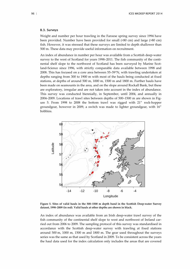
96 | ICES WKDEEP REPORT 2014
B.3. Surveys
Weight and number per hour trawling in the Faroese spring survey since 1994 have been provided. Number have been provided for small (<80 cm) and large (>80 cm) fish. However, it was stressed that these surveys are limited to depth shallower than 500 m. These data may provide useful information on recruitment.
An index of abundance in number per hour was available from a Scottish deep-water survey to the west of Scotland for years 1998–2011. The fish community of the conti-nental shelf slope to the northwest of Scotland has been surveyed by Marine Scot-land-Science since 1996, with strictly comparable data available between 1998 and 2008. This has focused on a core area between 55–59°N, with trawling undertaken at depths ranging from 300 to 1900 m with most of the hauls being conducted at fixed stations, at depths of around 500 m, 1000 m, 1500 m and 1800 m. Further hauls have been made on seamounts in the area, and on the slope around Rockall Bank, but these are exploratory, irregular and are not taken into account in the index of abundance. This survey was conducted biennially, in September, until 2004, and annually in 2004–2009. Locations of trawl sites between depths of 500–1500 m are shown in Fig-ure 5. From 1998 to 2008 the bottom trawl was rigged with 21” rock-hopper groundgear, however in 2009, a switch was made to lighter groundgear, with 16” bobbins.
Figure 5. Sites of valid hauls in the 500–1500 m depth band in the Scottish Deep-water Survey dataset, 1998–2009 (in red). Valid hauls at other depths are shown in black.
An index of abundance was available from an Irish deep-water trawl survey of the fish community of the continental shelf slope to west and northwest of Ireland car-ried out from 2006 to 2009. The sampling protocol of this survey was standardised in accordance with the Scottish deep-water survey with trawling at fixed stations around 500 m, 1000 m, 1500 m and 1800 m. The gear used throughout the surveys series was the same as that used by Scotland in 2009. To be consistent across the years the haul data used for the index calculation only includes the areas that are covered
-14 -12 -10 -8 -6 -4
54
55
56
57
58
59
60
Longitude
Latit
ude
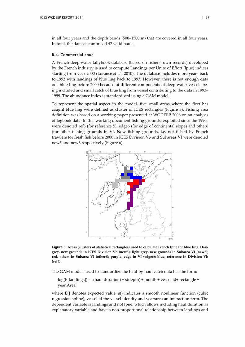
ICES WKDEEP REPORT 2014 | 97
in all four years and the depth bands (500–1500 m) that are covered in all four years. In total, the dataset comprised 42 valid hauls.
B.4. Commercial cpue
A French deep-water tallybook database (based on fishers’ own records) developed by the French industry is used to compute Landings per Unite of Effort (lpue) indices starting from year 2000 (Lorance et al., 2010). The database includes more years back to 1992 with landings of blue ling back to 1993. However, there is not enough data one blue ling before 2000 because of different components of deep-water vessels be-ing included and small catch of blue ling from vessel contributing to the data in 1993–1999. The abundance index is standardized using a GAM model.
To represent the spatial aspect in the model, five small areas where the fleet has caught blue ling were defined as cluster of ICES rectangles (Figure 3). Fishing area definition was based on a working paper presented at WGDEEP 2006 on an analysis of logbook data. In this working document fishing grounds, exploited since the 1990s were denoted ref5 (for reference 5), edge6 (for edge of continental slope) and other6 (for other fishing grounds in VI. New fishing grounds, i.e. not fished by French trawlers for fresh fish before 2000 in ICES Division Vb and Subareas VI were denoted new5 and new6 respectively (Figure 6).
60°
55°
50°
60°
55°
50°
0° 5° 10° 15° 20°
0° 5° 10° 15° 20°
64°0'N 24°0'W
49°0'N 4°0'E
Figure 6. Areas (clusters of statistical rectangles) used to calculate French lpue for blue ling. Dark grey, new grounds in ICES Division Vb (new5); light grey, new grounds in Subarea VI (new6); red, others in Subarea VI (other6); purple, edge in VI (edge6); blue, reference in Division Vb (ref5).
The GAM models used to standardize the haul-by-haul catch data has the form:
log(E[landings]) = s(haul duration) + s(depth) + month + vessel.id+ rectangle + year:Area
where E[] denotes expected value, s() indicates a smooth nonlinear function (cubic regression spline), vessel.id the vessel identity and year:area an interaction term. The dependent variable is landings and not lpue, which allows including haul duration as explanatory variable and have a non-proportional relationship between landings and

98 | ICES WKDEEP REPORT 2014
fishing time. The fit was done assuming a Tweedie distribution of the dependent variable with a log-link function using the mgcv package in R (Wood, 2006).
The Tweedie distribution has mean μ and variance φμp, where φ is a dispersion pa-rameter and p is called the index. As a Poisson-Gamma compound distribution was used, 1<p<2, the index p could not be estimated simultaneously with the model pa-rameters. In 2010, a detailed study was carried out and p=1.3 provided the best fit (Lorance et al., 2010).
In 2009, the model fit was restricted to haul durations from 60 to 300 minutes and depth 200–1100 m covering the species depth range and excluding too short and long hauls for which there are a few data. This lpue standardisation method allowed esti-mating lpue time-trends for the five small areas. The model provided lpue time-trends for the five areas. To derive standardized estimates for the whole study zone, lpue values are predicted for January, for all rectangles in each area (using the aver-age haul depth in each rectangle), a 5-h haul duration, and a vessel that operated during the whole period as prediction variables. Predictions for the entire study zone were then derived as the weighted average of the five area (rectangle average) esti-mates, with the weights being the number of rectangles in each area (Lorance et al., 2010). Some changes occurred in the fishery: protection areas for bleu ling spawning were introduced in 2009. As these limited the possibility for fishing for blue ling in these areas, hauls carried out throughout the time-series were excluded. The small areas new5 and new6 were not fished in 2011 by vessels contributing to the tally-books. As a result, the index for based upon the catch in three areas only. The depth and haul duration range was adjusted to reduce the confidence limits of the estimat-ed. Depth range of 500–1200 m and duration of 120–480 minutes were used. The change in these selections impacts little the estimates but reduce the confidence lim-its.
B.5. Other relevant data
No other relevant.
C. Assessment: data and method
Two assessment methods are used for this stock. A model call multiyear catch curve (MYCC) which is a random effects population dynamics model based on proportion-at-age and removal is used to estimate the total mortality and an age-structured Stock Reduction Analysis (SRA) is used to assess the trajectory in the population biomass over the catch history starting from 1966. International landings were small before the early 1970s so that biomass in the 1960s can be considered at of close to unexploited levels.
Multiyear catch curve
The multiyear catch curve model was carried out to estimate total annual mortality Zt taking account of interannual variations in recruitment. The data used are propor-tions-at-age in numbers by year and total catch (landings) in numbers by year.
The population dynamics in numbers are modelled as:
TtAaaeNN rZ
tatat .........11
1,1, =≤≤= +−
−−−
(1) 1)( 1,1,1,−
+++
−−−− += tZ
tAtAtA eNNN (2)
ICES WKDEEP REPORT 2014 | 99
where Na,t are population numbers-at-age a in year t, A+ is an age plus group and Zt are annual total ~mortality rates. Recruitment-at-age ar is assumed to vary randomly over time following a lognormal distribution
TtσμRRN Rttt 1),logN(~ R,1 == (3)
where μR is the mean recruitment and σR the standard deviation. For ease of interpre-tation the coefficient of variation (CVR) instead of σR was calculated making use of the fact that var(ln(x)) ≈ ln(CV(x)²+1). Recruitment is treated as a random effect in mod-el fitting.
Annual total mortality Zt is modelled by a random effect using a random walk over time:
TtσεεZZ tttt 1)N(0,~ Z1 =+= − (4)
The initial state vector at the beginning of year t=1 is calculated assuming constant historic total mortality Z0= M + F0
+−+− ≤<= AaaReN raa
Zaaa r
r1
)(1,
0
(5)
where F0 is constant historic fishing mortality.
The initial numbers in the plus group NA+,1 are estimated by an infinite sum over pre-vious years.
The observation model has two parts, the first one for population numbers-at-age Ya,t and the second for total catch in numbers. Numbers-at-age, assumed to follow a mul-tinomial distribution.
TtAaamY rtta 1),Multinom(p ~ ta,, =≤≤ + (6)
where pa,t are proportions-at-age and mt is the effective sample size in year t. Due to the clustered nature of individuals, the sample size in trawl surveys or harbour sam-pling programs does not correspond to the number of individuals measured but is rather much smaller (Pennington and Vølstad, 1994). As a result the observed varia-bility is much larger than would be expected given the number of measurements. Therefore the effective sample size was estimated from the sampling data using a Dirichlet-multinomial distribution and the dirmult package in R by Twedebrin272 k, Twedebrink (2009).
The second observation model for the total catch (in numbers) which is assumed to follow a Gamma distribution with parameters α and β.
Ct ~ Gamma(α,β) (7)
∑−−−
= taZ
t
tt Ne
ZMZCE t
,)1)((][ (8)
The coefficient of variation (CVc) of the Gamma distribution is related to the α param-eter as CVc=1/sqrt(α) and β = α /E[Ct]. The model is parameterised in terms of CVc.
Not all model parameters θ={Z0,..., Zt, M, F0, μR, σR, NA+,1, CVR, CVc} can be estimated and some need to be fixed. The fixed parameters where set as follows:
• natural mortality M=0.18 • coefficient of variation of landings or catch (CVc=0.05) to allow for some
misreporting
100 | ICES WKDEEP REPORT 2014
Estimation of free model parameters θ is carried out by maximum likelihood based on the observation vector y = (C1,..., CT, Yar,T,,..., YA+,T) which has conditional density fө (y | u,v) where u = (R1,..., Rn) is the vector of the latent random recruitment variable with marginal density h(u ) v=(Z1,………,ZT-1) is the total mortality random effect variable with marginal density g(v). The marginal likelihood function is obtained by integrating out u and v from the joint density L
∫∫= )()()()(),()( vyuyvguhvuyfθ θθθL (9)
The double integral in (9) is evaluated using the Laplace approximation as imple-mented in the random effects module of AD Model builder and described in Skaug and Fournier (2006). AD Model builder automatically calculates standard deviations of estimates based on the observed Fisher Information matrix.
For the analysis the data are restricted to the fully recruited age classes, 9 and over, a plus group is set at-age 19, called 19+.
Stock Reduction Analysis: SRA
Stock reduction analysis (SRA) is a developed form of delay-difference model (Quinn and Deriso, 1999). The method uses biological parameters and information for time delays due to growth and recruitment to predict the basic biomass dynamics of age structured populations without requiring information on age structure.. A descrip-tion of the general approach can be found in Kimura and Tagart (1982), Kimura et al. (1984) and Kimura (1985 and 1988).
The aim of stock reduction analysis is to estimate past and present biomass for a fish-ery. Three types of input data are required: biological parameters, abundance indices, and a complete catch history.
SRA is an iterative process, which operates with the following steps:
• A biomass B0 of the stock at the beginning of the catch history (initial bio-mass) is chosen;
• The stock biomass over the time-series is calculated by forward projection using, at each time-step the stock–recruitment relationship (derived from the input steepness), the natural mortality and removal to calculate num-ber-at-age at the start of the next time interval;
• The catchability q of each time-series of biomass index and the coefficient of variation c of the index are calculated;
• The likelihood of the value of B0 and q is calculated.
These four steps are repeated for a range of B0 and the B0 that maximises the likeli-hood of observed abundance indices is retained.
Implicit assumptions of this age-structured SRA include that (i) there is no density-dependence in growth and natural mortality, (ii) the stock–recruitment relationship is of the Beverton and Holt type.
Software used: FLaspm
FLaspm is a package for the statistical computing environment R (R Development Core Team, 2010). The package is open source and is currently hosted at GoogleCode (the source code is freely available at http://code.google.com/p/deepfishman/. FLaspm is part of the FLR project (Kell et al., 2007) and requires that the package FLCore is also installed (v >2.3). The stock reduction model used in this analysis implements the
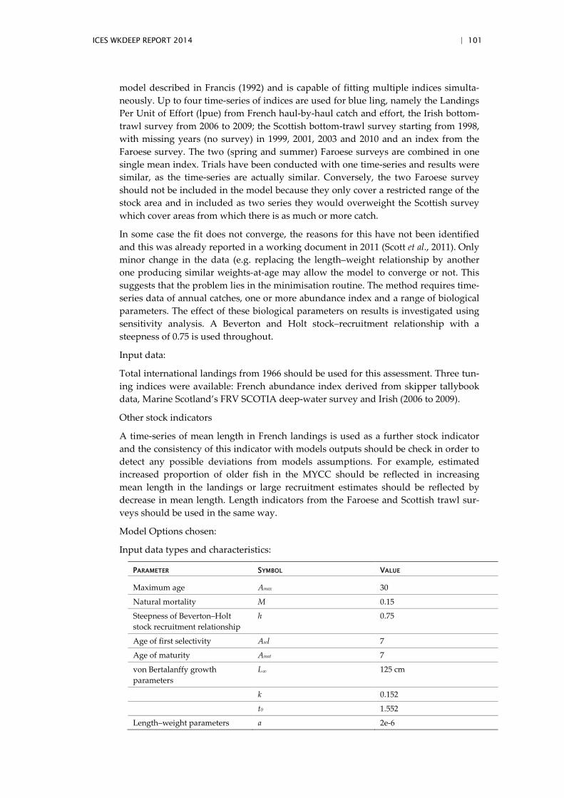
ICES WKDEEP REPORT 2014 | 101
model described in Francis (1992) and is capable of fitting multiple indices simulta-neously. Up to four time-series of indices are used for blue ling, namely the Landings Per Unit of Effort (lpue) from French haul-by-haul catch and effort, the Irish bottom-trawl survey from 2006 to 2009; the Scottish bottom-trawl survey starting from 1998, with missing years (no survey) in 1999, 2001, 2003 and 2010 and an index from the Faroese survey. The two (spring and summer) Faroese surveys are combined in one single mean index. Trials have been conducted with one time-series and results were similar, as the time-series are actually similar. Conversely, the two Faroese survey should not be included in the model because they only cover a restricted range of the stock area and in included as two series they would overweight the Scottish survey which cover areas from which there is as much or more catch.
In some case the fit does not converge, the reasons for this have not been identified and this was already reported in a working document in 2011 (Scott et al., 2011). Only minor change in the data (e.g. replacing the length–weight relationship by another one producing similar weights-at-age may allow the model to converge or not. This suggests that the problem lies in the minimisation routine. The method requires time-series data of annual catches, one or more abundance index and a range of biological parameters. The effect of these biological parameters on results is investigated using sensitivity analysis. A Beverton and Holt stock–recruitment relationship with a steepness of 0.75 is used throughout.
Input data:
Total international landings from 1966 should be used for this assessment. Three tun-ing indices were available: French abundance index derived from skipper tallybook data, Marine Scotland’s FRV SCOTIA deep-water survey and Irish (2006 to 2009).
Other stock indicators
A time-series of mean length in French landings is used as a further stock indicator and the consistency of this indicator with models outputs should be check in order to detect any possible deviations from models assumptions. For example, estimated increased proportion of older fish in the MYCC should be reflected in increasing mean length in the landings or large recruitment estimates should be reflected by decrease in mean length. Length indicators from the Faroese and Scottish trawl sur-veys should be used in the same way.
Model Options chosen:
Input data types and characteristics:
PARAMETER SYMBOL VALUE
Maximum age Amax 30
Natural mortality M 0.15
Steepness of Beverton–Holt stock recruitment relationship
h 0.75
Age of first selectivity Asel 7
Age of maturity Amat 7
von Bertalanffy growth parameters
L∞ 125 cm
k 0.152
t0 1.552
Length–weight parameters a 2e-6
102 | ICES WKDEEP REPORT 2014
b 3.15
D. Short-Term Projection
No short-term prediction are carried out for this stock.
E. Medium-Term Projections
None.
F. Long-Term Projections
None.
G. Biological Reference Points
No biological reference points defined.
H. Other Issues
The stock identity is an issue for blue ling. The only area were juvenile are known to occur in high number in the Icelandic shelf. No juvenile are known to occur in Subar-eas VI and VII and number observed in the Faroese survey (about one fish smaller than 80 cm per hour) do not seem sufficient to supply the abundance for adult blue ling.
H.1. Historical overview of previous assessment methods
Exploratory assessment carried out far are summarised below (synthesis carried out as part of the DEEPFISHMAN project).
YEAR ASSESSMENT
TYPE3 METHOD ASSESSMENT PACKAGE/
PROGRAM USED USED
FOR
ADVICE?
IF NOT, WHAT WAS
LATEST SCIENTIFIC
ADVICE BASED ON?
1998 Exploratory Schaefer& DeLury depletion model
CEDA (1) No French OTB and Faroese longline lpue
2000 Exploratory Schaefer& DeLury depletion model
CEDA (1) No French OTB unstandardised lpue
2004 Exploratory Schaefer, Pella- Tomlinson and Fox production models & DeLury depletion model
CEDA (1) No Trend in French commercial otter trawl lpue
Exploratory Stock reduction PMOD No Trend in French commercial otter trawl lpue
2006 Exploratory Catch Survey CSA (Mesnil, 2003) No Trend in French commercial otter
3 Exploratory, Benchmark (to identify best practise), Update (repeat of previous years’ assessment using same method and settings but with the addition of data for another year).

ICES WKDEEP REPORT 2014 | 103
analysis trawl lpue
(1) MRAG (UK) software.
104 | ICES WKDEEP REPORT 2014
Summary of data ranges used in recent assessments:
DATA 2007 ASSESSMENT 2008 ASSESSMENT 2009 ASSESSMENT 2010 ASSESSMENT
Landings Years: 1988–2006 Years: 1988–2007 Years: 1966-2008 Years: 1966–2009
Quarterly length dist. of French landings
Years: 1989–2006 Years: 1984–2007 Years: 1984–2008 Years: 1984–2010
Quarterly length dist. of Faroese landings
Years: 1995–2006 Years: 1995–2007 Years: 1995–2008 Years: 1995–2009
Quartely age dist.
Year: 2009
Survey: Scottish deep-water
Years: 1998-2008 N° per hour
Years: 1998–2009 N° per hour
Survey: Irish Years: 2006–2009 N° per hour
Survey: spring and autumn Faroese
Years: 1994–2009 N° per hour Size
Haul-by-haul lpues from French trawlers
Not used Not used Years: 2000-2008 Years: 2000–2009
Aggregated unstandardised French lpue
Years: 1989–2006 Years: 1989–2007 Years: 1989–2008 Not used
I. References Annala, J. H., and Sullivan, K. J. 1996. Report from the Fishery assessment plenary, April-May
1996: stock assessments and yield estimates. 308 pp.
Bridger, J. P. 1978. New deep-water trawling grounds to the West of Britain. Laboratory Leaf-let, Ministry of Agriculture Fisheries and Food (MAFF), Directorate of Fisheries Research, Lowestoft, United Kingdom.
Dorel, D. 1986. Poissons de l’Atlantique Nord-Est. Relations Taille-Poids. DRV-86-001/RH/NANTES, 183 pp. (available at http://Archimer.ifremer.fr).
Ehrich, S. 1983. On the occurrence of some fish species at the slopes of the Rockall Trough. Archiv für Fischereiwissenschaft, 33: 105–150.
Hewitt, D. A., and Hoenig, J. M. 2005. Comparison of two approaches for estimating natural mortality based on longevity. Fishery Bulletin, 103: 433–437.
Hilborn, R., and Walters, C.J. 1992. Quantitative Fisheries Stock Assessment – Choice, Dynam-ics and Uncertainty. New York & London. Chapman & Hall.
Hoenig, J. M. 1983. Empirical use of longevity data to estimate mortality rates. Fish. Bull. 82:898–903.
Kell, L. T., Mosqueira,I,. Grosjean, P., Fromentin, J., Garcia, Hillary, R., Jardim, E., Mardle, S., Pastoors, M. A., Poos, J. J., Scott, F. and Scott, R. D., 2007, FLR: An open-source framework for the evaluation and development of management strategies, ICES Journal of Marine Science, 64(4), 640–646.
Kimura, D.K., and Tagart, J.V. 1982. Stock reduction analysis, another solution to the catch equations. Canadian Journal of Fisheries and Aquatic Sciences, vol. 3 no. 11, pp 1467–1472.
ICES WKDEEP REPORT 2014 | 105
Kimura, D.K., Balsiger, J.W., Ito, D.H. 1984. Generalised stock reduction analysis. Canadian Journal of Fisheries and Aquatic Sciences, vol. 41, no. 9, pp 1325–1333.
Kimura, D.K. 1985. Changes to stock reduction analysis indicated by Schnute’s general theory. Canadian Journal of Fisheries and Aquatic Sciences, vol. 42, no. 12, pp 2059–2060.
Kimura, D.K. Stock–recruitment curves as used in the stock reduction analysis model. 1988. J. CONS. CIEM., vol. 44, no. 3, pp 253–258.
Large, P.A. 2002. The use of stock reduction analysis to assess deep-water species in the ICES area – an initial investigation (WD to ICES WGEEP, 2002).
Large, P. A., Diez, G., Drewery, J., Laurans, M., Pilling, G. M., Reid, D. G., Reinert, J., South, A. B., and Vinnichenko, V. I. 2010. Spatial and temporal distribution of spawning aggrega-tions of blue ling (Molva dypterygia) west and northwest of the British Isles. ICES Journal of Marine Science, 67: 494–501.
Lorance, P., Pawlowski, L., and Trenkel, V. M. 2009. Deriving blue ling abundance indices from industry haul by haul data. ICES Annual Science Conference, Berlin, 21–25 September 2009, ICES CM 2009/L:12, 25 pp.
Lorance, P., Pawlowski, L., and Trenkel, V. M. 2010. Standardizing blue ling landings per unit effort from industry haul-by-haul data using generalized additive models. ICES Journal of Marine Science, 67: 1650–1658.
Lorance, P., Agnarsson, S., Damalas, D., des Clers, S., Figueiredo, I., Gil, J., and Trenkel, V. M. 2011. Using qualitative and quantitative stakeholder knowledge: examples from European deep-water fisheries. ICES Journal of Marine Science, 68: 1815–1824. Lorance, P., Agnars-son, S., Damalas, D., des Clers, S., Figueiredo, I., Gil, J., and Trenkel, V. M. 2011. Using qualitative and quantitative stakeholder knowledge: examples from European deep-water fisheries. ICES Journal of Marine Science, 68: 1815–1824.
Magnussen, E. 2007. Interpopulation comparison of growth patterns of 14 fish species on Faroe Bank: are all fishes on the bank fast-growing? Journal of Fish Biology, 71: 453–475.
Magnússon, J. V., and Magnússon, J. 1995. The distribution, relative abundance, and biology of the deep-sea fishes of the Icelandic slope and Reykjanes Ridge. In: Hopper, A. G., Deep-water fisheries of the North Atlantic oceanic slope. Kluwer Academic Publishers, Dor-drecht/Boston/London, 161–199.
Mesnil, B. 2003. The Catch-Survey Analysis (CSA) method of fish stock assessment: an evalua-tion using simulated data. Fisheries Research (Amsterdam), 63: 193–212.
Moguedet, P. 1988. Approche de la dynamique de stocks accessoires : Le cas des lingues (Molva spp.) exploitées par la flottille industrielle Lorientaise. Université des Sciences et Tech-niques de Lille Flandre Artois, Lille, 301.
Ofstad, L.H. 2013. Info about length distributions and cpue from groundfish surveys and commercial catches for blue ling in Faroese waters (Vb), Faroe Marine Research Institute, WD to WGDEEP 2013, 8pp.
Quinn T.J. and Deriso R.B. 1999. Quantitative Fish Dynamics. Oxford University Press. New York. 1999. 542p.
R Development Core Team. 2010. R: A Language and Environment for Statistical Computing, R Foundation for Statistical Computing, Vienna, Austria.
Scott, F. Lorance, P. and Large, P. 2011. Exploratory assessment using stock reduction analysis to assess blue ling (Molva dypterygia) in Vb, VI, VII. (WD submitted to ICES WGEEP, 2011).
Wood, S. N. 2006. Generalized additive models. An introduction with R. Chapman & Hall/CRC, Boca Raton.
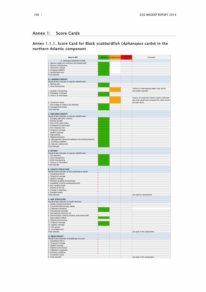
106 | ICES WKDEEP REPORT 2014
Annex 1: Score Cards
Annex 1.1.1. Score Card for Black scabbardfish (Aphanopus carbo) in the northern Atlantic component
How to fill? No bias Potential bias Confirmed bias Comment
A. SPECIES IDENTIFICATION1. Species subject to confusion and trained staff2. Species misreporting3. Taxonomic change4. Grouping statistics5. Identification KeyFinal indicator
B. LANDINGS WEIGHTRecall of bias indicator on species identification1. Missing part2. Area misreporting
3. Quantity misreportingcatches in international waters may not be accurately reported
4. Population of vessels5. Source of information
6. Conversion factor
Source of conversion factors used is unknown. Any bias would have remained the same across the time series
7. Percentage of mixed in the landings8. Damaged fish landedFinal indicator
C. DISCARDS WEIGHTRecall of bias indicator on species identification1. Sampling allocation scheme2. Raising variable3. Size of the catch effect4. Damaged fish discarded5. Non response rate6. Temporal coverage7. Spatial coverage8. High grading9. Slipping behaviour10. Management measures leading to discarding behaviour11. Working conditions12. Species replacementFinal indicator
D. EFFORTRecall of bias indicator on species identification1. Unit definition2. Area misreporting3. Effort misreporting4. Source of informationFinal indicator
E. LENGTH STRUCTURERecall of bias indicator on discards/landing weight1. Sampling protocol2. Temporal coverage3. Spatial coverage4. Random sampling of boxes/trips5. Availability of all the landings/discards6. Non sampled strata7. Raising to the trip8. Change in selectivity9. Sampled weightFinal indicator not used for assessment
F. AGE STRUCTURERecall of bias indicator on length structure1. Quality insurance protocol2. Conventional/actual age validity3. Calibration workshop4. International exchange5. International reference set6. Species/stock reading easiness and trained staff7. Age reading method8. Statistical processing9. Temporal coverage10. Spatial coverage11. Plus group12. Incomplete ALKFinal indicator not used in the assessment
G. MEAN WEIGHTRecall of bias indicator on length/age structure1. Sampling protocol2. Temporal coverage3. Spatial coverage4. Statistical processing5. Calibration equipment6. Working conditions7. Conversion factor8. Final indicator not used in the assessment
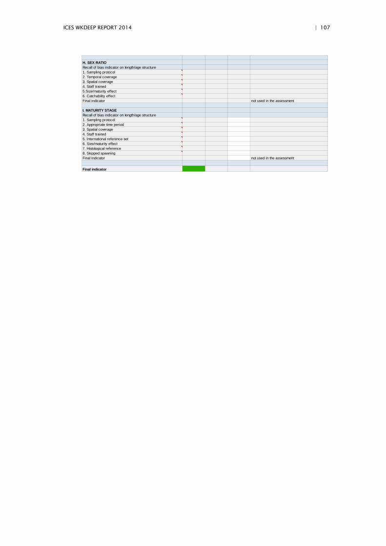
ICES WKDEEP REPORT 2014 | 107
H. SEX RATIORecall of bias indicator on length/age structure1. Sampling protocol2. Temporal coverage3. Spatial coverage4. Staff trained5.Size/maturity effect6. Catchability effectFinal indicator not used in the assessment
I. MATURITY STAGERecall of bias indicator on length/age structure1. Sampling protocol2. Appropriate time period3. Spatial coverage4. Staff trained5. International reference set6. Size/maturity effect7. Histological reference8. Skipped spawningFinal indicator not used in the assessment
Final indicator
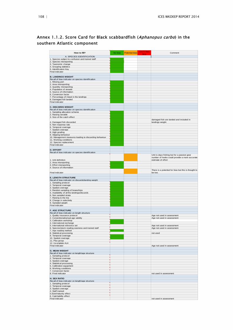
108 | ICES WKDEEP REPORT 2014
Annex 1.1.2. Score Card for Black scabbardfish (Aphanopus carbo) in the southern Atlantic component
How to fill? No bias Potential bias Confirmed bias Comment
A. SPECIES IDENTIFICATION1. Species subject to confusion and trained staff2. Species misreporting3. Taxonomic change4. Grouping statistics5. Identification KeyFinal indicator
B. LANDINGS WEIGHTRecall of bias indicator on species identification1. Missing part2. Area misreporting3. Quantity misreporting4. Population of vessels5. Source of information6. Conversion factor7. Percentage of mixed in the landings8. Damaged fish landedFinal indicator
C. DISCARDS WEIGHTRecall of bias indicator on species identification1. Sampling allocation scheme2. Raising variable3. Size of the catch effect
4. Damaged fish discardeddamaged fish are landed and included in landings weight.
5. Non response rate6. Temporal coverage7. Spatial coverage8. High grading9. Slipping behaviour10. Management measures leading to discarding behaviour11. Working conditions12. Species replacementFinal indicator
D. EFFORTRecall of bias indicator on species identification
1. Unit definition
Unit is days fishing but for a passive gear number of hooks could provide a more accurate estimate of effort
2. Area misreporting3. Effort misreporting4. Source of information
Final indicatorThere is a potential for bias but this is thought to be low.
E. LENGTH STRUCTURERecall of bias indicator on discards/landing weight1. Sampling protocol2. Temporal coverage3. Spatial coverage4. Random sampling of boxes/trips5. Availability of all the landings/discards6. Non sampled strata7. Raising to the trip8. Change in selectivity9. Sampled weightFinal indicator
F. AGE STRUCTURERecall of bias indicator on length structure1. Quality insurance protocol Age not used in assessment 2. Conventional/actual age validity Age not used in assessment 3. Calibration workshop4. International exchange5. International reference set Age not used in assessment 6. Species/stock reading easiness and trained staff Age not used in assessment 7. Age reading method8. Statistical processing not used9. Temporal coverage10. Spatial coverage11. Plus group12. Incomplete ALKFinal indicator Age not used in assessment
G. MEAN WEIGHTRecall of bias indicator on length/age structure1. Sampling protocol2. Temporal coverage3. Spatial coverage4. Statistical processing5. Calibration equipment6. Working conditions7. Conversion factor8. Final indicator not used in assessment
H. SEX RATIORecall of bias indicator on length/age structure1. Sampling protocol2. Temporal coverage3. Spatial coverage4. Staff trained5.Size/maturity effect6. Catchability effectFinal indicator not used in assessment

ICES WKDEEP REPORT 2014 | 109
I. MATURITY STAGERecall of bias indicator on length/age structure1. Sampling protocol2. Appropriate time period3. Spatial coverage4. Staff trained5. International reference set6. Size/maturity effect7. Histological reference8. Skipped spawningFinal indicator not used in assessment
Final indicator
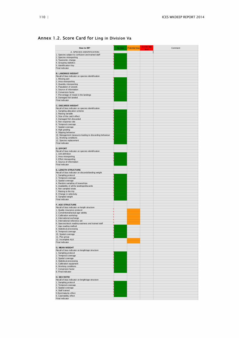
110 | ICES WKDEEP REPORT 2014
Annex 1.2. Score Card for Ling in Division Va
How to fill? No bias Potential bias Confirmed bias Comment
A. SPECIES IDENTIFICATION1. Species subject to confusion and trained staff2. Species misreporting3. Taxonomic change4. Grouping statistics5. Identification KeyFinal indicator
B. LANDINGS WEIGHTRecall of bias indicator on species identification1. Missing part2. Area misreporting3. Quantity misreporting4. Population of vessels5. Source of information6. Conversion factor7. Percentage of mixed in the landings8. Damaged fish landedFinal indicator
C. DISCARDS WEIGHTRecall of bias indicator on species identification1. Sampling allocation scheme2. Raising variable3. Size of the catch effect4. Damaged fish discarded5. Non response rate6. Temporal coverage7. Spatial coverage8. High grading9. Slipping behaviour10. Management measures leading to discarding behaviour11. Working conditions12. Species replacementFinal indicator
D. EFFORTRecall of bias indicator on species identification1. Unit definition2. Area misreporting3. Effort misreporting4. Source of informationFinal indicator
E. LENGTH STRUCTURERecall of bias indicator on discards/landing weight1. Sampling protocol2. Temporal coverage3. Spatial coverage4. Random sampling of boxes/trips5. Availability of all the landings/discards6. Non sampled strata7. Raising to the trip8. Change in selectivity9. Sampled weightFinal indicator
F. AGE STRUCTURERecall of bias indicator on length structure1. Quality insurance protocol2. Conventional/actual age validity3. Calibration workshop4. International exchange5. International reference set6. Species/stock reading easiness and trained staff7. Age reading method8. Statistical processing9. Temporal coverage10. Spatial coverage11. Plus group12. Incomplete ALKFinal indicator
G. MEAN WEIGHTRecall of bias indicator on length/age structure1. Sampling protocol2. Temporal coverage3. Spatial coverage4. Statistical processing5. Calibration equipment6. Working conditions7. Conversion factor8. Final indicator
H. SEX RATIORecall of bias indicator on length/age structure1. Sampling protocol2. Temporal coverage3. Spatial coverage4. Staff trained5.Size/maturity effect6. Catchability effectFinal indicator

ICES WKDEEP REPORT 2014 | 111
I. MATURITY STAGERecall of bias indicator on length/age structure1. Sampling protocol2. Appropriate time period3. Spatial coverage4. Staff trained5. International reference set6. Size/maturity effect7. Histological reference8. Skipped spawningFinal indicator
Final indicator
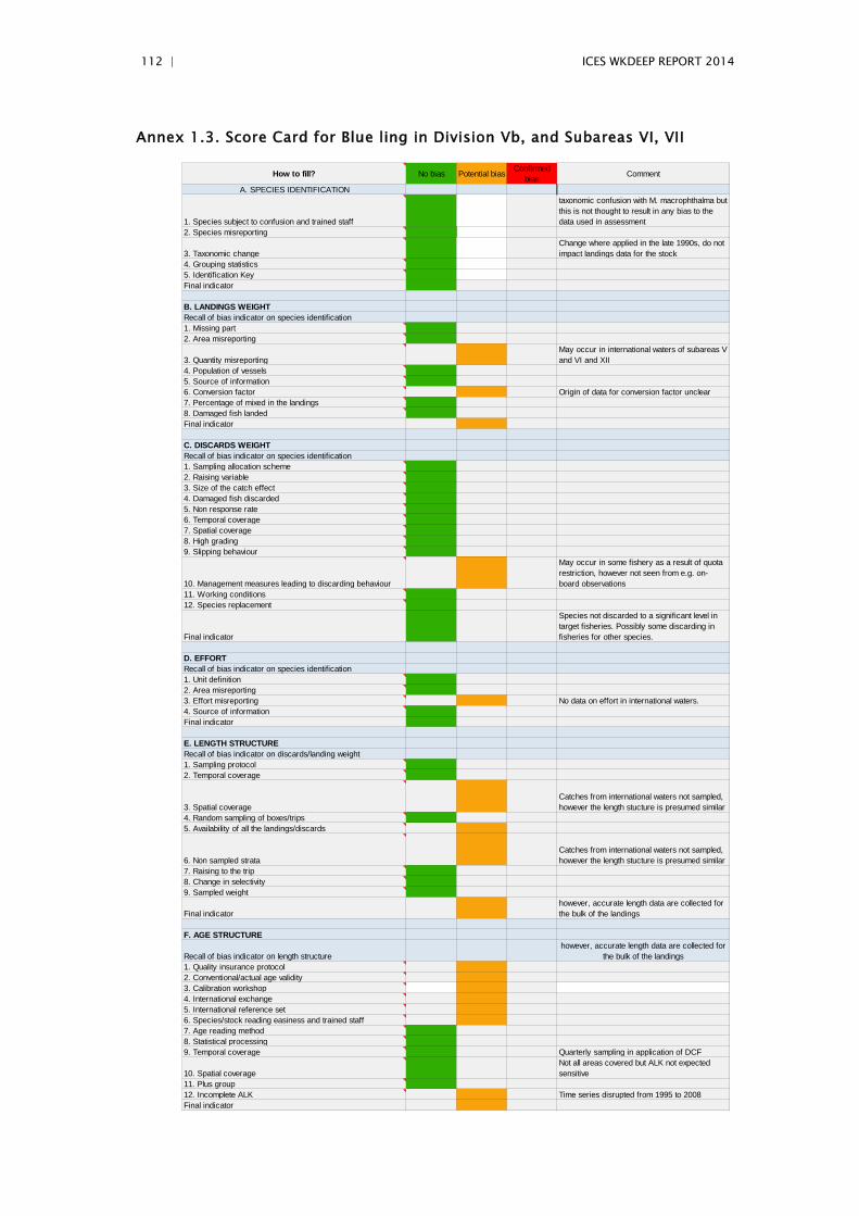
112 | ICES WKDEEP REPORT 2014
Annex 1.3. Score Card for Blue ling in Division Vb, and Subareas VI, VII
How to fill? No bias Potential bias Confirmed bias Comment
A. SPECIES IDENTIFICATION
1. Species subject to confusion and trained staff
taxonomic confusion with M. macrophthalma but this is not thought to result in any bias to the data used in assessment
2. Species misreporting
3. Taxonomic changeChange where applied in the late 1990s, do not impact landings data for the stock
4. Grouping statistics5. Identification KeyFinal indicator
B. LANDINGS WEIGHTRecall of bias indicator on species identification1. Missing part2. Area misreporting
3. Quantity misreportingMay occur in international waters of subareas V and VI and XII
4. Population of vessels5. Source of information6. Conversion factor Origin of data for conversion factor unclear7. Percentage of mixed in the landings8. Damaged fish landedFinal indicator
C. DISCARDS WEIGHTRecall of bias indicator on species identification1. Sampling allocation scheme2. Raising variable3. Size of the catch effect4. Damaged fish discarded5. Non response rate6. Temporal coverage7. Spatial coverage8. High grading9. Slipping behaviour
10. Management measures leading to discarding behaviour
May occur in some fishery as a result of quota restriction, however not seen from e.g. on-board observations
11. Working conditions12. Species replacement
Final indicator
Species not discarded to a significant level in target fisheries. Possibly some discarding in fisheries for other species.
D. EFFORTRecall of bias indicator on species identification1. Unit definition2. Area misreporting3. Effort misreporting No data on effort in international waters.4. Source of informationFinal indicator
E. LENGTH STRUCTURERecall of bias indicator on discards/landing weight1. Sampling protocol2. Temporal coverage
3. Spatial coverageCatches from international waters not sampled, however the length stucture is presumed similar
4. Random sampling of boxes/trips5. Availability of all the landings/discards
6. Non sampled strataCatches from international waters not sampled, however the length stucture is presumed similar
7. Raising to the trip8. Change in selectivity9. Sampled weight
Final indicatorhowever, accurate length data are collected for the bulk of the landings
F. AGE STRUCTURE
Recall of bias indicator on length structurehowever, accurate length data are collected for
the bulk of the landings1. Quality insurance protocol2. Conventional/actual age validity3. Calibration workshop4. International exchange5. International reference set6. Species/stock reading easiness and trained staff7. Age reading method8. Statistical processing9. Temporal coverage Quarterly sampling in application of DCF
10. Spatial coverageNot all areas covered but ALK not expected sensitive
11. Plus group12. Incomplete ALK Time series disrupted from 1995 to 2008Final indicator
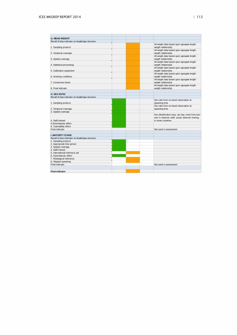
ICES WKDEEP REPORT 2014 | 113
G. MEAN WEIGHTRecall of bias indicator on length/age structure
1. Sampling protocolAll weigth data based upon agregate length-weigth relationship
2. Temporal coverageAll weigth data based upon agregate length-weigth relationship
3. Spatial coverageAll weigth data based upon agregate length-weigth relationship
4. Statistical processingAll weigth data based upon agregate length-weigth relationship
5. Calibration equipmentAll weigth data based upon agregate length-weigth relationship
6. Working conditionsAll weigth data based upon agregate length-weigth relationship
7. Conversion factorAll weigth data based upon agregate length-weigth relationship
8. Final indicatorAll weigth data based upon agregate length-weigth relationship
H. SEX RATIORecall of bias indicator on length/age structure
1. Sampling protocolSex ratio from on-board observation at spawning time
2. Temporal coverageSex ratio from on-board observation at spawning time
3. Spatial coverage
4. Staff trained
Sex identification easy, pb may come from tunr-over in observer staff, yearly observer training in some countries
5.Size/maturity effect6. Catchability effectFinal indicator Not used in assessment
I. MATURITY STAGERecall of bias indicator on length/age structure1. Sampling protocol2. Appropriate time period3. Spatial coverage4. Staff trained5. International reference set6. Size/maturity effect7. Histological reference8. Skipped spawningFinal indicator Not used in assessment
Final indicator
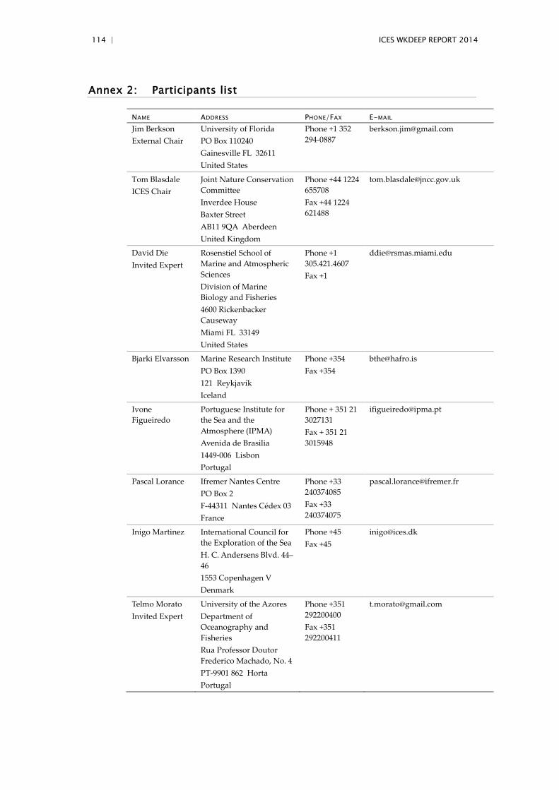
114 | ICES WKDEEP REPORT 2014
Annex 2: Participants list
NAME ADDRESS PHONE/FAX E-MAIL Jim Berkson External Chair
University of Florida PO Box 110240 Gainesville FL 32611 United States
Phone +1 352 294-0887
Tom Blasdale ICES Chair
Joint Nature Conservation Committee Inverdee House Baxter Street AB11 9QA Aberdeen United Kingdom
Phone +44 1224 655708 Fax +44 1224 621488
David Die Invited Expert
Rosenstiel School of Marine and Atmospheric Sciences Division of Marine Biology and Fisheries 4600 Rickenbacker Causeway Miami FL 33149 United States
Phone +1 305.421.4607 Fax +1
Bjarki Elvarsson Marine Research Institute PO Box 1390 121 Reykjavík Iceland
Phone +354 Fax +354
Ivone Figueiredo
Portuguese Institute for the Sea and the Atmosphere (IPMA) Avenida de Brasilia 1449-006 Lisbon Portugal
Phone + 351 21 3027131 Fax + 351 21 3015948
Pascal Lorance Ifremer Nantes Centre PO Box 2 F-44311 Nantes Cédex 03 France
Phone +33 240374085 Fax +33 240374075
Inigo Martinez International Council for the Exploration of the Sea H. C. Andersens Blvd. 44–46 1553 Copenhagen V Denmark
Phone +45 Fax +45
Telmo Morato Invited Expert
University of the Azores Department of Oceanography and Fisheries Rua Professor Doutor Frederico Machado, No. 4 PT-9901 862 Horta Portugal
Phone +351 292200400 Fax +351 292200411

ICES WKDEEP REPORT 2014 | 115
NAME ADDRESS PHONE/FAX E-MAIL
Mike Park For NSRAC Scottish White Fish Producers Association Limited North Lodge, 11, Bath St. AB39 2DH Stonehaven United Kingdom
Phone +44 7710504773
Gudmundur Thordarson
Marine Research Institute
PO Box 1390
121 Reykjavík
Iceland
Phone +354 5752000
Fax +354 5752001
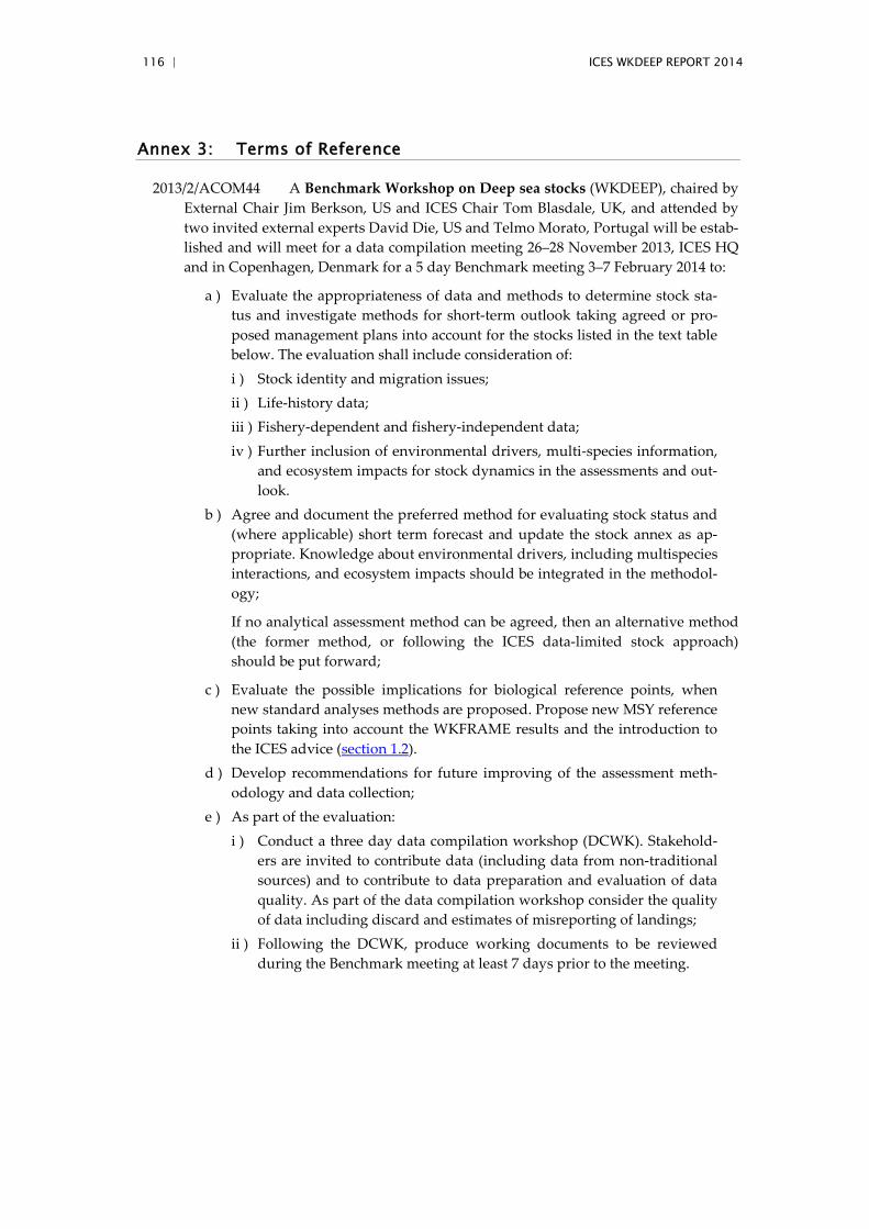
116 | ICES WKDEEP REPORT 2014
Annex 3: Terms of Reference
2013/2/ACOM44 A Benchmark Workshop on Deep sea stocks (WKDEEP), chaired by External Chair Jim Berkson, US and ICES Chair Tom Blasdale, UK, and attended by two invited external experts David Die, US and Telmo Morato, Portugal will be estab-lished and will meet for a data compilation meeting 26–28 November 2013, ICES HQ and in Copenhagen, Denmark for a 5 day Benchmark meeting 3–7 February 2014 to:
a ) Evaluate the appropriateness of data and methods to determine stock sta-tus and investigate methods for short-term outlook taking agreed or pro-posed management plans into account for the stocks listed in the text table below. The evaluation shall include consideration of: i ) Stock identity and migration issues; ii ) Life-history data; iii ) Fishery-dependent and fishery-independent data; iv ) Further inclusion of environmental drivers, multi-species information,
and ecosystem impacts for stock dynamics in the assessments and out-look.
b ) Agree and document the preferred method for evaluating stock status and (where applicable) short term forecast and update the stock annex as ap-propriate. Knowledge about environmental drivers, including multispecies interactions, and ecosystem impacts should be integrated in the methodol-ogy;
If no analytical assessment method can be agreed, then an alternative method (the former method, or following the ICES data-limited stock approach) should be put forward;
c ) Evaluate the possible implications for biological reference points, when new standard analyses methods are proposed. Propose new MSY reference points taking into account the WKFRAME results and the introduction to the ICES advice (section 1.2).
d ) Develop recommendations for future improving of the assessment meth-odology and data collection;
e ) As part of the evaluation: i ) Conduct a three day data compilation workshop (DCWK). Stakehold-
ers are invited to contribute data (including data from non-traditional sources) and to contribute to data preparation and evaluation of data quality. As part of the data compilation workshop consider the quality of data including discard and estimates of misreporting of landings;
ii ) Following the DCWK, produce working documents to be reviewed during the Benchmark meeting at least 7 days prior to the meeting.
ICES WKDEEP REPORT 2014 | 117
STOCK ASSESSMENT LEAD WG
bli-5b67
Blue ling in Division Vb, and Subareas VI, VII
WGDEEP
Lin-icel Ling in Division Va WGDEEP
bsf-nrtn Black scabbardfish (Aphanopus carbo) in Subareas VI, VII and Divisions Vb and XIIb
WGDEEP
bsf-89 Black scabbardfish (Aphanopus carbo) in Subareas VIII and IX
WGDEEP
bsf-oth Black scabbardfish (Aphanopus carbo) in other areas (Subareas I, II, IV, X, XIV and Divisions IIIa, Vb)
WGDEEP
The Benchmark Workshop will report by 1 April 2014 for the attention of ACOM.