Embed Size (px)
Citation preview

NOT FOR QUOTATION WITHOUT THE PERXISSIOK OF THE AUTHOR
IDENTIFIABLE AGE, PERIOD, AND COHORT EFFECTS: A n Exploratory Approach Applied to Ita l ian Female Mortality
J o h n R. Witmoth
October 1985 WP-95-69
This r e s e a r c h w a s conducted in conjunction with a summer r e s e a r c h seminar on heterogeneity dynamics, under t h e di rect ion of James W. Vaupel and Anatoli I. Yashin, in t h e Population Program at IIASA led by Nathan Keyfitz.
Working Papers are interim r e p o r t s on work of t h e International Insti tute f o r Applied Systems Analysis and have received only limited review. Views o r opinions expressed here in d o not necessar i ly r e p r e s e n t those of t h e Insti tute o r of i t s National Member Organizations.
INTERNATIONAL INSTITUTE FOR APPLIED SYSTEMS ANALYSIS 2361 Laxenburg, Austria

ACKNOWLEDGMENTS
This work w a s made possible, above all , by t h e interaction and spir i t of cooperative e f for t which were presen t in IIASA's YSSP population group. All par- ticipants, whether program d i rec tors , young scientists, o r visitors, provided valu- able ideas and inspiration. Particularly useful suggestions and comments were made by Andrew Foster, Bill Hodges, and Mike Stoto. Jim Vaupel, both f o r his knowledge of t h e subject and his enthusiasm f o r t he present r e sea rch , deserves special recognition.
A special word of thanks also goes t o Graziella Caselli, who knows be t t e r than anyone else how these da ta were collected, and who gave much help, both in data- re la ted questions, and in more substantive interpretations.

FOREWORD
A group of eleven Ph.D. candidates from seven countries--Robin Cowan, An- drew Foster, Nedka Gateva, William Hodges, Arno Kitts, Eva Lelievre, Fernando Rajulton, Lucky Tedrow, Marc Tremblay, John Wilmoth, and Zeng Yi--worked togeth- e r at IIASA from June 17 through September 6, 1985, in a seminar on population heterogeneity. The seminar was led by the two of us with the help of Nathan Key- fitz, leader of t h e Population Program, and Bradley Gambill, Dianne Goodwin, and Alan Bernstein, r e s e a r c h e r s in t he Population Program, as well as the occasional participation of guest scholars at IIASA, including Michael Stoto, Sergei Scherbov, Joel Cohen, Frans Willekens, Vladimir Crechuha, and Geer t Ridder. Susanne Stock, o u r s ec re t a ry , and Margaret Traber , managed the seminar superbly.
Each of the elevent students in t he seminar succeeded in writing a r e p o r t on the research they had done. With only one exception, t he students evaluated the seminar as "very productive"; the exception thought i t w a s "productive". The two of us agree: the quality of the research produced exceeded o u r expectations and made the summer a thoroughly enjoyable experience. We were particularly pleased by the interest and sparkle displayed in ou r daily, hour-long colloquium, and by the sp i r i t of cooperation all the participants, both students and more senior r e sea rche r s , displayed in generously sharing ideas and otherwise helping each other .
One of t he best of t he r e sea rch r epor t s produced and probably the most ori- ginal is the r e p o r t by John Wilmoth tha t appears in this working paper . Building on some of the work on the mathematics of population surfaces, on the use of shaded contour maps f o r displaying population surfaces, and on Italian mortality tha t had been s ta r ted at IIASA by the two of us and W. Brian Arthur, Bradley A. Gambill, and Graziella Caselli, Wilmoth developed an approach f o r analyzing age, period, and cohort effects t ha t shows considerable promise f o r f u r t h e r development and appli- cation. This r e p o r t thus exemplifies the productive ro le IIASA can play in bringing together diligent, creat ive scholars from different countries and disciplines.
James W. Vaupel Anatoli I. Yashin
I D E N T m L E AGE, PERIOD. AND COHORT EFFECTS: An Exploratory Approach Applied to
I ta l i an Female Mortality
J o h n R. WiLmoth
Office of Population Research Pr inceton University
Pr inceton, New J e r s e y 08544 USA
I t i s of g r e a t in te res t t o s e p a r a t e demographic t r e n d s into t h r e e components:
age , per iod, and c o h o r t ef fects . To what ex ten t i s mortality at a g e a and time t af-
f ec ted by t h e a g e of t h e individuals, t h e events of t h e p r e s e n t day, and t h e l ife his-
t o r y of t h e c o h o r t now a g e a? Of specia l i n t e r e s t i s t h e t h i r d component: Can
c o h o r t s c a r r y t h e i r level of mortality with them? To what e x t e n t does high/low
mortality e a r l y in l ife lead t o high/low mortality l a t e r in life? If a c o h o r t i s disad-
vantage in childhood, c a n th i s e a r l y selection cause i t t o b e a n advantaged c o h o r t
l a t e in life?
Severa l a u t h o r s have discussed t h e importance of childhood mortality reduc-
t ions in t h e his tor ical improvements observed l a t e r in t h e l ives of t h e affected
cohor ts . Kermack, McKendrick, and McKinlay (1934) studied dea th rates in
nineteenth-century England and Wales and found c l e a r cohort-specific mortality
reductions. Coale and Kisker (1985) update th i s e a r l y work and c o r r o b o r a t e t h e
findings. They emphasize t h e importance of d a t a quali ty, especially at o lder ages ,
in any such analysis. P r e s t o n and Van d e Walle (1978) show similar r e s u l t s in
French u rban mortali ty in t h e nineteenth century. Horiuchi (1983) s tudies t h e
mortality of w a r su rv ivors in Japan, Germany, France, and o t h e r countr ies , and
finds h igher levels of mortality l a t e r in l ife f o r men who were in adolescence at t h e
end of t h e wars. Caselli and Capocaccia (forthcoming), studying Ital ian d a t a , link
high mortality e a r l y in l ife with high levels in middle age. They show, however,
t h a t t h e s e e f fec t s tend t o decline in importance a f t e r a g e 45.

Other authors have discussed the possibility of an inverse relationship
between mortality in ear ly childhood and mortality at advanced ages. Meindl
(1982) finds such a relationship in studying nineteenth century r u r a l New England
communities. Vaupel, Manton, and Stallard (1979) and Vaupel and Yashin (1985)
emphasize the theory of heterogeneity and selection as a means of explaining the
phenomenon. McMillan and N a m (1985) give a comprehensive review of the l i tera-
t u re on mortality crossovers and conclude tha t such crossovers a r e not mere ar-
tifactual phenomena.
In this work we attempt t o define clearly what is meant by age, period, and
cohort effects, and propose a graphical method of decomposition which may help t o
shed some light on these hotly-debated issues. The method is applied t o Italian fe-
male mortality da ta f o r t he period, 1869-1978, and very c l ea r cohor t and period
variations in mortality are observed.
2. DEFINITIONS OF AGE. PEEUOD. AND COHORT EFFECTS
We must f i r s t consider t he fac tors which influence the level of mortality,
k ( a , t ) , f o r a given age a and time t. Many people have spoken of age-period-
cohort models of mortality, but what exactly is meant by these t h r e e fac tors is
often unclear. In this pape r we a r e interested in t he mortality of a national popu-
lation, so a period is one calendar year of time, age r e f e r s t o the time from birth
f o r an individual o r cohort , and a cohort is a group of people born in a single
calendar year . The ultimate source of difficulty is tha t t he t h r e e fac tors are re-
lated: a person who is age a a t time t was obviously born at time t-a, if w e think,
f o r the moment, in continuous age and time. Knowing any two of these th ree fac-
to rs , then, allows us unambiguously t o know the third one as well.
This interrelationship between age, period, and cohort variables is the source
of a well-known identification problem. If observed mortality, ~ ( a , t ) , is decreas-
ing with time, we cannot know whether this i s because progress against mortality is
being made now, a t time t, o r because the cohort born at time t-a i s advantaged
compared t o the preceding cohort . If k ( a , t ) increases with age, we cannot know
whether this is due t o a natural tendency f o r mortality t o increase with age, o r
again because the cohort from time t-a i s advantaged compared t o t he preceding
cohort (who i s now slightly older). Finally, if ~ ( a , t ) tends t o increase with respec t
t o both age and time together (that is, in the cohort direction), we cannot deter-
mine how much of t he increase i s due t o aging and how much is a t t r ibutable t o
period change.
In o r d e r t o define cohor t and period effects in a way which can be measured,
i t i s best t o consider not just simple age effects, which reflect some constant age-
specific contribution to mortality, but t o think in t e r m s of the changing age s t ruc-
t u r e of mortality. This would be a mortality sur face which would re f lec t t he age
pa t te rn of mortality as i t is influenced by the smooth, long-term t rends in mortali-
ty. This age s t ruc tu re of mortality would be a function of both the cohor t and
period t rends in mortality.
For any one fixed point in time, to, t he curve p ( a , to ) would take on the fami-
l i a r bathtub shape. ~ d r any age, a o , p ( a o , t ) would show a steady (though not
necessarily constant) rate of change. The changing shape of p ( a , t ) would re f lec t
the changing, underlying age pa t te rn of mortality. The essential requirement,
though, is t ha t this be a smooth sur face in all directions, which, for o u r purposes,
will mean tha t i t must have smooth f i r s t derivatives.
W e make no attempt, then, t o explain why this pa t t e rn changes. There would
be many factors t o be considered. For example, health and medical p rogress would
be important components, but p rogress at one age may mean higher mortiality l a t e r
in life for the affected cohor t s due t o heterogeneity and selection (Vaupel and
Yashin, 1985). Again, though, w e see tha t measuring the effehts of selection versus
long-term period progress is a non-identifiable problem. If r e a l mortality progress
is g r e a t e r at younger than at older ages, is i t due t o heterogeneity and selection
operating on the cohorts who are now at advanced ages, or i s i t simply tha t the
health progress now being made favors t he younger age groups?
I t seems tha t answers t o such questions will have t o come from study of the
biological mechanisms of aging in t he presence of a changing health environment,
which is beyond the scope of this paper . For this reason, w e do not concern our-
selves with such questions. Rather , w e let all long-term mortality t rends (whether
they be period o r cohor t t rends) be ref lected in t he changing age s t ruc tu re of
mortality, which gives t he expected mortality rate f o r a given age and time. W e
then consider deviations between the observed and expected rates.
The cohort effects which in te res t us, then, are deviations which occu r in a
cohort-specific pat tern. To the extent tha t w e find a deviation at the point, ( a , t ),
which is similar t o those at ( a + l , t +I), ( a +2,t +2), etc . , w e may conclude tha t
t h e r e are rea l , identifiable cohor t effects in operation. If t he cohor t variations
are such tha t t he observed mortality is lower than the expected, w e say t ha t a
cohort is advantaged . Likewise, a cohort is d i sadvan taged if observed mortality
is higher than expected.
Similarly, period variations a r e deviations which follow a period-specific pat-
t e rn . A deviation at ( a , t ) which resembles the deviations a t ( a +1, t ), ( a +2, t ),
e tc . , is a period effect. A positive deviation (observed g r e a t e r than expected) will
be call an unYavorabLe period, while a negative deviation (observed less than ex-
pected) will be called a YavorabLe period.
In both cases , these period and cohort variations a r e relative effects, in tha t
they a r e relative t o the overall t rend of mortality, which is contained in what we
have already defined as the changing age s t ruc tu re of mortality. The crux of the
age-period-cohort identification problem is the question of how much of this trend
should be at t r ibuted t o periods and how much t o cohorts. Our approach in this pa-
p e r is tha t i t is t he relative effects (i.e., the variations around the t rend) which
a r e of interest , and we make no attempt t o separa te the overall t rend of mortality
into what may be i ts period and cohort components. (Caselli and Capocaccia, in a
forthcoming paper , take a similar approach in considering a range of reasonable
cohort and period trends.)
3. MATHEMATICAL FORMULATION
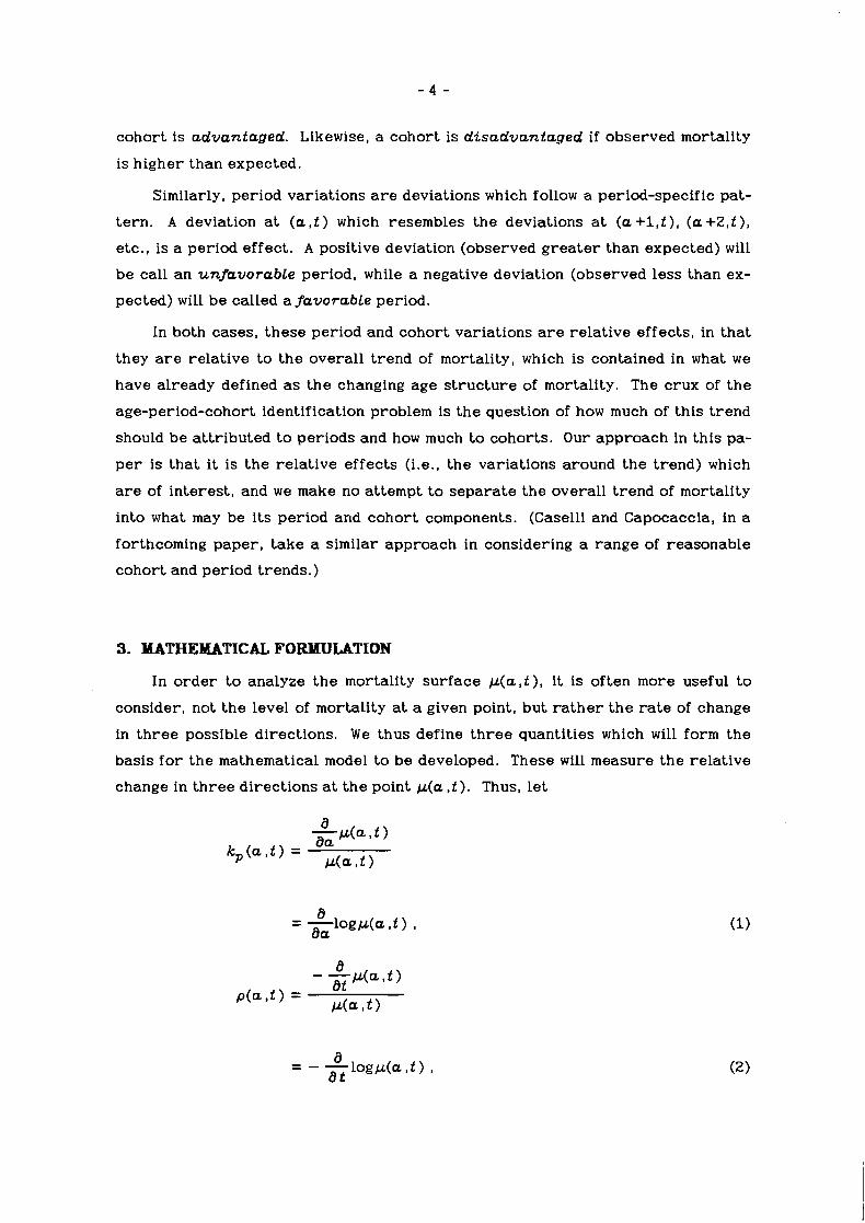
In o r d e r t o analyze the mortality surface p ( a , t ) , i t is often more useful t o
consider, not the level of mortality a t a given point, but r a t h e r the r a t e of change
in t h ree possible directions. We thus define t h r e e quantities which will form the
basis f o r the mathematical model t o be developed. These will measure the relative
change in t h ree directions at t h e point p ( a , t ) . Thus, l e t
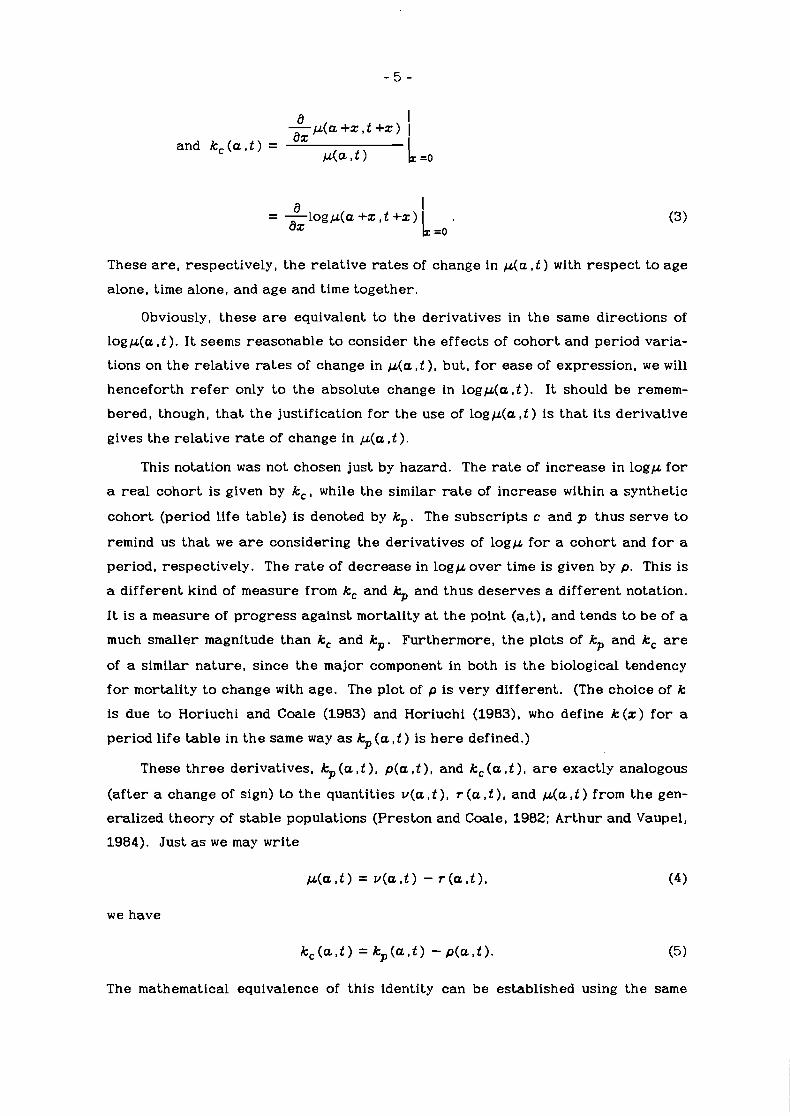
a I @ ( a +Z , t +z) I
and k , ( a , t ) = az @(a rt h =o
These a r e , respectively, the relat ive rates of change in p ( a , t ) with r e spec t to age
alone, time alone, and age and time together .
Obviously, these are equivalent to the derivatives in the same directions of
logp(a , t ). I t s e e m s reasonable t o consider the effects of cohor t and period varia-
tions on the relat ive rates of change in p ( a , t ), but, f o r ease of expression, w e will
henceforth refer only t o the absolute change in l ogp (a , t ) . I t should be r e m e m -
bered, though, t ha t t he justification for the use of l o g p ( a , t ) i s t ha t i t s derivative
gives the relat ive rate of change in @(a , t ).
This notation w a s not chosen just by hazard. The rate of increase in l ogp f o r
a r e a l cohort is given by k c , while t he similar rate of increase within a synthetic
cohort (period life table) is denoted by kp. The subscr ipts c and p thus s e r v e t o
remind us tha t w e are considering the derivatives of l o g p f o r a cohor t and f o r a
period, respectively. The rate of decrease in l o g p ove r time is given by p. This i s
a different kind of measure from kc and kp and thus deserves a different notation.
I t i s a measure of p rogress against mortality at the point (a,t) , and tends to be of a
much smaller magnitude than kc and kp. Furthermore, t he plots of kp and kc are
of a similar nature , since t he major component in both is t he biological tendency
f o r mortality t o change with age. The plot of p is very different. (The choice of k
is due to Horiuchi and Coale (1983) and Horiuchi (1983), who define k (z) f o r a
period life table in t he same way as kp ( a , t ) is h e r e defined.)
These t h r e e derivatives, kp ( a , t ), p(a , t ) , and kc ( a , t ), are exactly analogous
(a f te r a change of sign) to the quantities v (a , t ), r ( a , t ), and p ( a , t ) from t h e gen-
eralized theory of stable populations (Preston and Coale, 1982; Arthur and Vaupel,
1984). Just as w e may write
we have
k c ( a , t ) = k p ( a , t ) - p ( a , t ) . ( 5 )
The mathematical equivalence of this identity can be established using the same
methods given in the sources cited, s o the proof will not be repeated here . In-
stead, an intuitive, demographic explanation will be attempted.
The derivative, kp ( a , t ), represents the tendency fo r mortality increase (or
decrease) within a synthetic cohort (i.e., period). Similarly, kc ( a , t ) expresses
the r a t e of mortality increase ( o r decrease) within a r e a l cohort. Finally, pro-
gress against mortality is contained in p ( a , t ) . If mortality is constant, then
p ( a , t )=0, and kc ( a , t )=kp ( a , t ). This means tha t a person who is age a at time t is
expected t o experience the same mortality increase as expressed in the appropri-
ate period life table f o r t ha t time. If p ( a , t ) is non-zero, though, progress against
mortality is being made (though i t may actually be negative "progress"), and the
actual mortality experience of the individual at ( a , t ) will ref lect the period pat-
t e rn of mortality, kp, less any progress being made, p. That is, t he equation,
is equivalent t o t he expression,
cohort mortality increase = period mortality increase - progress against mortality.
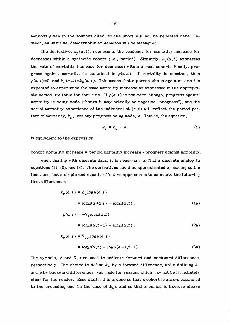
When dealing with d iscre te data , i t is necessary t o find a discrete analog t o
equations ( I ) , (Z), and (3). The derivatives could be approxtmated by moving spline
functions, but a simple and equally effective approach is to calculate the following
f i r s t differences:
The symbols, A and V, are used t o indicate forward and backward differences,
respectively. The choice t o define kp by a forward difference, while defining kc
and p by backward differences, w a s made f o r reasons which may not be immediately
c l ea r f o r the r eade r . Essentially, this is done s o tha t a cohort is always compared
t o the preceding one (in the case of kp), and s o tha t a period is likewise always
compared to the one just before (in the case of p and kc).
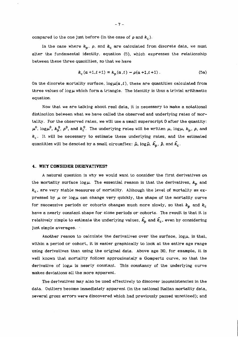
In the case where kp, p , and kc a r e calculated from discre te data , we must
a l t e r the fundamental identity, equation (5), which expresses the relationship
between these t h r e e quantities, so tha t we have
On the discrete mortality surface, logp(a , t ) , these a r e quantities calculated from
th ree values of l o g p which form a triangle. The identity is thus a trivial arithmetic
equation.
Now that we a r e talking about r e a l data , i t is necessary t o make a notational
distinction between what we have called the observed and underlying rates of mor-
tality. For t he observed r a t e s , w e will use a small superscr ipt 0 after the quantity:
pO, l o g g , ki, and k:. The underlying rates will be written p. logp. kp, p, and
kc. I t will be necessary t o estimate these underlying rates, and the estimated
quantities will be denoted by a small circumflex: fi. logfi. 5. 8, and 5,.
4. WHY CONSIDER DEEUYATIVES?
A natural question is why w e would want t o consider t he f i r s t derivatives on
the mortality surface logp. The essential reason is tha t the derivatives, kp and
kc, a r e very s table measures of mortality. Although t h e level of mortality as ex-
pressed by p o r l ogp can change very quickly, t he shape of t he mortality curve
f o r successive periods o r cohorts changes much more slowly, s o tha t kp and kc
have a nearly constant shape f o r close periods o r cohorts. The resul t is tha t i t is
relatively simple t o estimate the underlying values, gp and dc, even by considering
just simple averages. -
Another reason t o calculate the derivatives over t he surface, logp, is tha t ,
within a period o r cohort , i t is eas ie r graphically t o look a t the en t i re age range
using derivatives than using t h e original data. Above age 30, f o r example, i t i s
well known tha t mortality follows approximately a Gompertz curve, s o tha t the
derivative of logp i s nearly constant. This constancy of the underlying curve
makes deviations all the more apparent .
The derivatives may also be used effectively t o discover inconsistencies in t he
data . Outliers become immediately apparent (in the national Italian mortality data ,
several gross e r r o r s were discovered which had previously passed unnoticed); and

other peculiar tendencies become apparen t which are hidden in t he r a w data (the
Italian data again provides an example which will be discussed la te r ) .
Finally, taking t h e derivative of logp in one of t h e t h r e e directions becomes a
means of approximately removing one of t he t h r e e effects (i.e., age, period, o r
cohort) . This is t r u e only in a neighborhood around t h e age, period, o r cohort in-
volved, and remains valid only s o long a s t he change in t h e age s t ruc tu re of mor-
tality i s s l o w in t ha t neighborhood. It can be shown tha t , if p (a , t )=p(t ) i s constant
f o r all ages at any time t, then kp ( a , t ) = kp ( a ) does not change with time, and thus
kc ( a , t ) = kp ( a )-p(t ). Since this assumption should hold approximately in a neigh-
borhood around ( a , t ), and since p(a , t ) i s generally quite small, kp should change
li t t le f o r adjacent periods, and kc should change li t t le f o r adjacent cohorts.
Thus, in taking the derivative with respec t t o age and considering k: f o r adja-
cent periods, t h e deviations found in t h e various periods must be stochastic o r
resul t from cohor t variations in mortality (Horiuchi, 1983). Likewise, in taking t h e
derivative with r e spec t t o age and time and considering k: f o r adjacent cohorts ,
t he deviations found in t h e various cohorts must be random or resul t from period
variations in mortality. The derivative with respec t to time alone, will show,
above all , t h e confounding of cohort and period variations in mortality. In all
t h r e e cases , though, t h e derivatives will be affected by t h e overal l t rend of mor-
tality, p ( a , t ) , but this will be a relatively small effect , and, in a neighborhood
around ( a , t ) , an almost negligible one.
We may say, then, t ha t k: approximately removes period variations from t h e
observed data . Likewise, k: approximately removes cohort variations, and
nearly eliminates age effects. This is t h e final motivation f o r considering deriva-
t ives on t h e mortality sur face logp(a , t ) . They provide t h e f i r s t s t ep in a filtering
process which attempts t o effectively s epa ra t e long-term mortality t rends from
period and cohor t variations.
5. APPLICATION TO ITALIAN FEMALE MORTALITY DATA
In o r d e r to i l lustrate t h e technique of age-period-cohort decomposition just
described, w e will examine historical mortality da ta f o r Italian females. The data
are f o r t h e years 1869 t o 1978 and give observed, single-year, conditional proba-
bilities of death, q:, f o r ages 0-79. W e estimate t h e observed fo rce of mortality,
p0 (z ), by the simple equation,
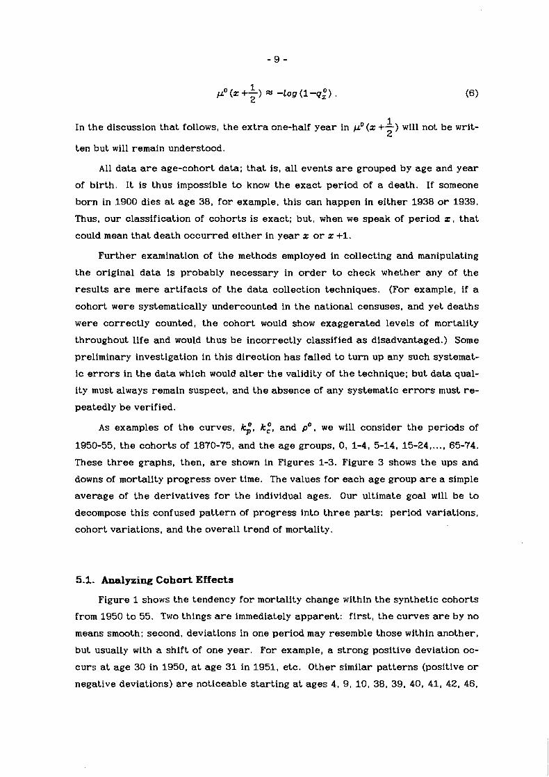
1 In the discussion tha t follows, the e x t r a one-half y e a r in po ( z +-) will not be writ-
2
ten but will remain understood.
All da ta are age-cohort data; t ha t is , all events are grouped by age and yea r
of bir th . I t i s thus impossible to know t h e exac t period of a death. If someone
born in 1900 dies at age 38, f o r example, this can happen in e i t he r 1938 or 1939.
Thus, o u r classification of cohor t s is exact ; but, when w e speak of period z , tha t
could mean tha t death occur red e i t he r in yea r z or x +l.
Fur ther examination of t h e methods employed in collecting and manipulating
the original da ta i s probably necessary in o r d e r to check whether any of t he
resu l t s are mere a r t i f ac t s of t h e da ta collection techniques. (For example, if a
cohort were systematically undercounted in t he national censuses, and yet deaths
were cor rec t ly counted, t h e cohort would show exaggerated levels of mortality
throughout life and would thus be incorrect ly classified as disadvantaged.) Some
preliminary investigation in this direction has failed to tu rn up any such systemat-
ic errors in t he da t a which would a l t e r t he validity of t h e technique; but da ta qual-
ity must always remain suspect , and t h e absence of any systematic errors must re-
peatedly be verified.
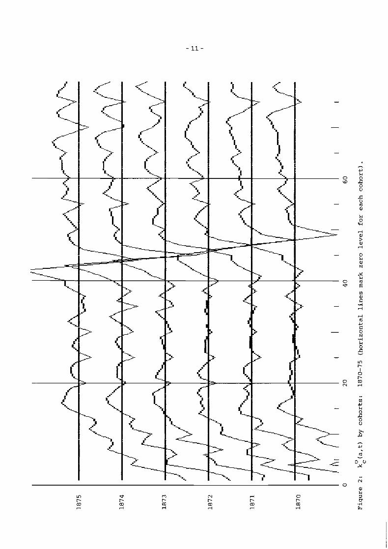
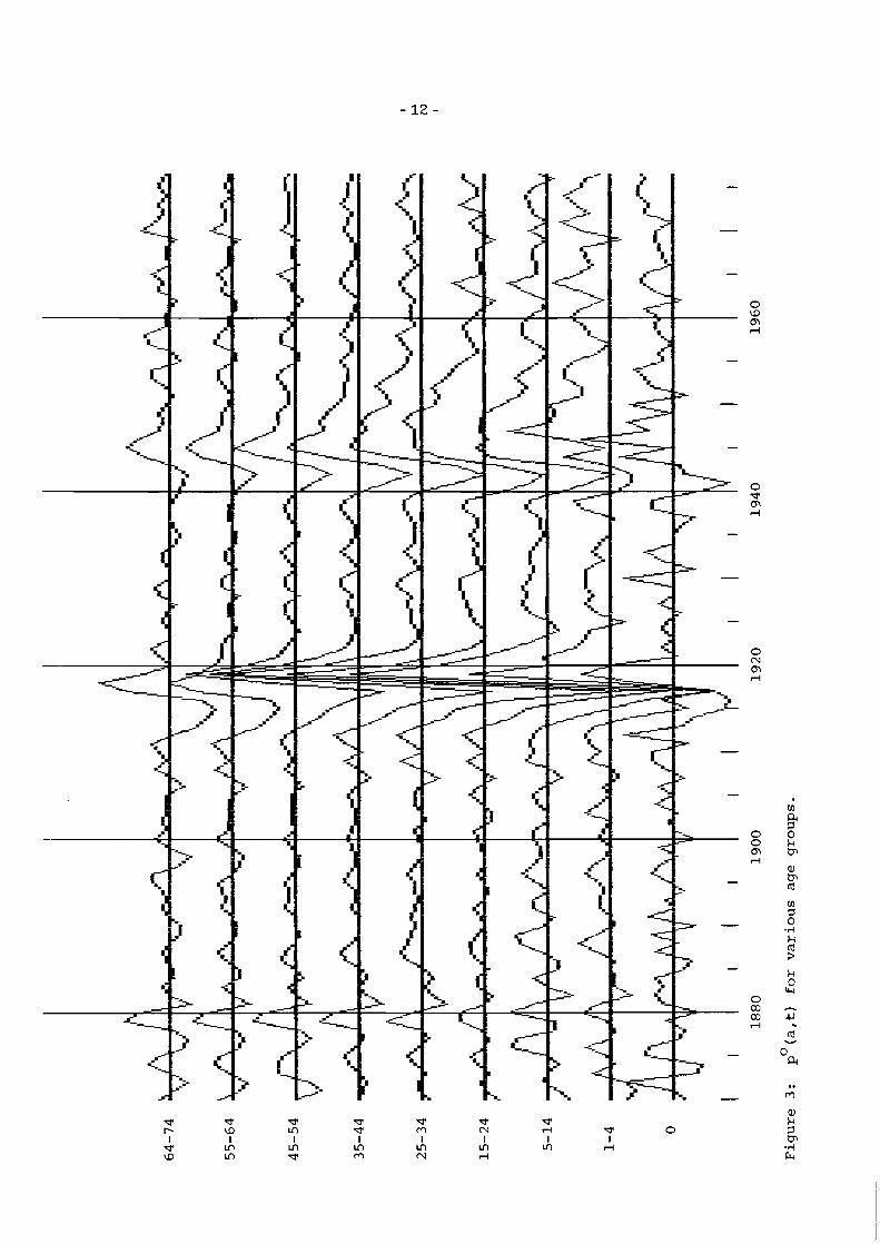
A s examples of t h e curves , k;, k:, and p O , w e will consider t h e periods of
1950-55, t h e cohor t s of 1870-75, and the age groups, 0, 1-4, 5-14, 15-24, ..., 65-74.
These t h r e e graphs, then, are shown in Figures 1-3. Figure 3 shows t h e ups and
downs of mortality progress ove r time. The values f o r each age group are a simple
average of t he der ivat ives for the individual ages. Our ultimate goal will be to
decompose th i s confused pa t t e rn of progress into t h r e e par ts : period variations,
cohor t variations, and t h e overal l t rend of mortality.
5.1. Analyzing Cohort Effects
Figure 1 shows t h e tendency f o r mortality change within t h e synthetic cohorts
from 1950 to 55. Two things are immediately apparent : f i r s t , t he curves are by no
means smooth; second, deviations in one period may resemble those within another ,
but usually with a shift of one year . For example, a s t rong positive deviation oc-
cu r s at age 30 in 1950, at age 31 in 1951, etc. Other similar pa t te rns (positive or
negative deviations) are noticeable s tar t ing at ages 4, 9 , 10 , 38, 39, 40, 41, 42, 46,
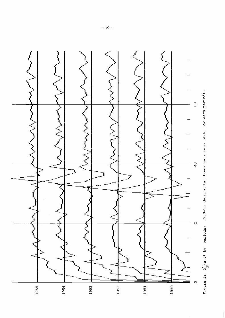
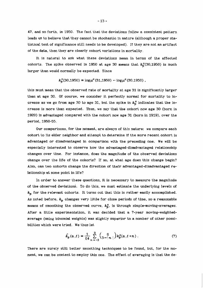
47, and s o for th , in 1950. The fac t tha t the deviations follow a consistent pa t te rn
leads us t o believe tha t they cannot be stochastic in nature (although a p rope r sta-
tistical t es t of significance sti l l needs t o be developed). If they a r e not an a r t i fac t
of the data, then they are clearly cohort variations in mortality.
It is natural t o ask what these deviations mean in t e r m s of the affected
cohorts. The spike observed in 1950 at age 30 means tha t k;(30,1950) is much
l a rge r than would normally be expected. Since
this must mean tha t the observed rate of mortality at age 31 is significantly l a rge r
than at age 30. Of course, w e consider i t perfectly normal f o r mortality t o in-
c r ease as w e go from age 30 t o age 31, but the spike in k; indicates tha t the in-
c r ease is more than expected. Thus, we say tha t the cohort now age 30 (born in
1920) is advantaged compared with the cohort now age 31 (born in 1919), over t he
period, 1950-55.
Our comparisons, f o r the moment, a r e always of this nature: w e compare each
cohort t o i ts e lder neighbor and attempt t o determine if t he more recent cohor t is
advantaged o r disadvantaged in comparison with the preceding one. W e will be
especially interested t o observe how the advantaged-disadvantaged relationship
changes over time. For instance, does the magnitude of the observed deviations
change over the life of the cohorts? If so, at what age does this change begin?
Also, can two cohorts change the direction of the i r advantaged-disadvantaged re-
lationship at some point in life?
In o r d e r t o answer these questions, i t is necessary t o measure the magnitude
of the observed deviations. To do this, we must estimate the underlying levels of
kp f o r t he relevant cohorts. I t tu rns out tha t this is r a t h e r easily accomplished.
A s noted before, kp changes very li t t le f o r close periods of time, s o a reasonable
means of smoothing the observed curve, k;, is through simple-moving-averages.
After a li t t le experimentation, i t was decided tha t a 7-year moving-weighted-
average (using binomial weights) w a s slightly superior t o a number of o the r possi-
bilities which were tr ied. W e thus let
There a r e surely still be t t e r smoothing techniques t o be found, but, f o r the mo-
ment, w e can be content t o employ this one. The effect of averaging is tha t the de-
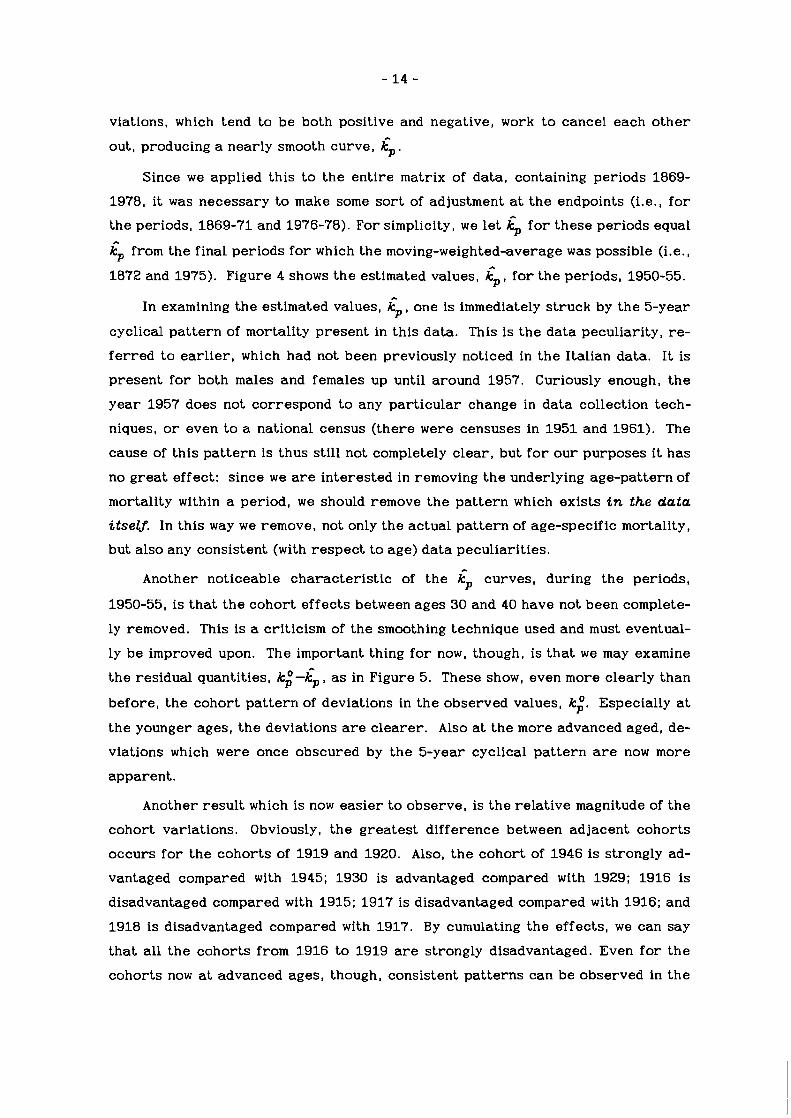
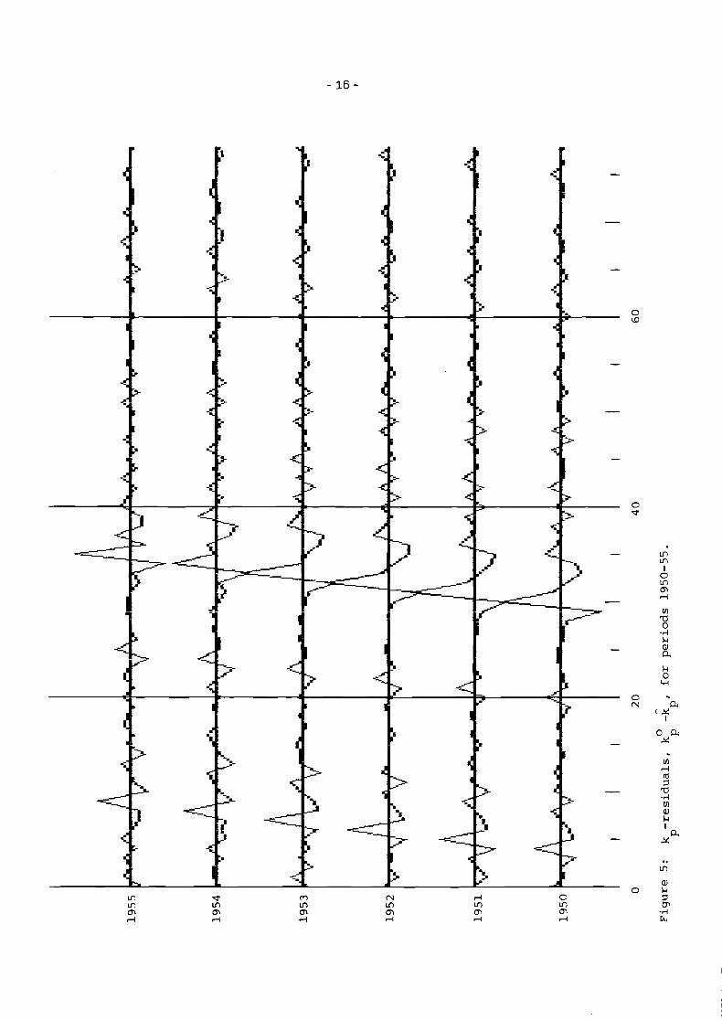
viations, which tend t o be both positive and negative, work to cancel each o t h e r
out, producing a nearly smooth curve, cp. Since w e applied this to t h e en t i re matrix of data , containing periods 1869-
1978, i t w a s necessary to make some sort of adjustment at t h e endpoints (i.e., f o r
the periods. 1869-71 and 1976-78). For simplicity. w e l e t & f o r these periods equal
4 from the final periods f o r which t h e moving-weighted-average w a s possible (i.e..
1872 and 1975). Figure 4 shows t h e estimated values. C p . f o r t he periods. 1950-55. A
In examining the estimated values, k p , one is immediately s t ruck by the 5-year
cyclical pa t te rn of mortality presen t in this data. This is t h e da ta peculiarity, re-
f e r r e d t o ea r l i e r , which had not been previously noticed in t h e Italian data. I t is
p resen t f o r both males and females up until around 1957. Curiously enough, t h e
y e a r 1957 does not correspond to any par t icular change in da ta collection tech-
niques, or even to a national census ( there were censuses in 1951 and 1961). The
cause of this pa t te rn is thus still not completely c l ea r , but for o u r purposes i t has
no g r e a t effect: since w e are interested in removing t h e underlying age-pattern of
mortality within a period, we should remove t h e pa t te rn which exis ts in the data
i tsel f . In this way w e remove, not only t he actual pa t te rn of age-specific mortality,
but a lso any consistent (with r e spec t to age) da t a peculiarities.
Another noticeable charac te r i s t ic of t h e Cp curves, during the periods.
1950-55, is t ha t t h e cohor t effects between ages 30 and 40 have not been complete-
ly removed. This is a criticism of t he smoothing technique used and must eventual-
ly be improved upon. The important thing f o r now, though, is t ha t w e may examine
t h e residual quantities. q - C p , as in Figure 5. These show, even more clear ly than
before , t h e cohor t pa t te rn of deviations in t h e observed values, k;. Especially at
t h e younger ages, t h e deviations are c l ea re r . Also at t h e more advanced aged, de-
viations which were once obscured by t h e 5-year cyclical pa t te rn are now more
apparent .
Another resu l t which is now eas i e r to observe, is t h e relat ive magnitude of t h e
cohor t variations. Obviously, t h e grea tes t difference between adjacent cohor t s
occurs f o r t h e cohor t s of 1919 and 1920. Also, t h e cohor t of 1946 is strongly ad-
vantaged compared with 1945; 1930 is advantaged compared with 1929; 1916 is
disadvantaged compared with 1915; 1917 is disadvantaged compared with 1916; and
1918 is disadvantaged compared with 1917. By cumulating the effects , w e can say
tha t all t h e cohor t s from 1916 to 1919 are strongly disadvantaged. Even f o r t h e
cohorts now a t advanced ages, though, consistent pa t te rns can be observed in t h e
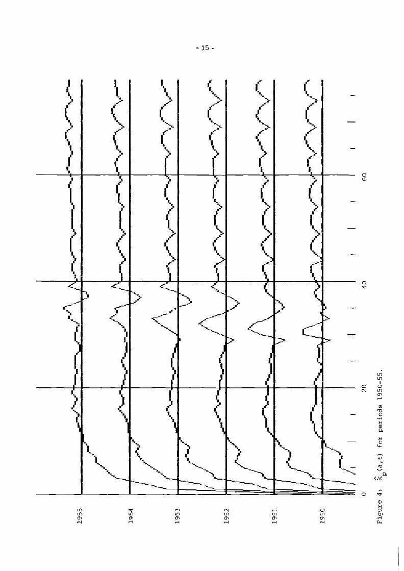
residuals, although t h e di f ferences are clear ly of a smaller magnitude.
To continue t h e analysis of cohor t ef fects , we can make a g r a p h of a l l t h e kp- *
residuals, k i -kp , using a program, called "Lexis", developed by Bradley Gambell
and James Vaupel at IIASA. This permits us t o see t h e overa l l p a t t e r n of t h e res i -
duals. For simplicity, we examine only t h e sign of t h e res iduals in Figure 6 .
The diagonal p a t t e r n of t h e residuals i s most s t r ik ing; fu r the rmore , i t is in-
teres t ing t o note t h a t t h e width of t h e diagonal l ines of ten encompasses only one or
two cohor ts . This would indicate t h a t t h e r e may b e c o h o r t var ia t ions in mortality
through a l a r g e por t ion of l ife which may b e observed even between ad jacen t
cohor ts .
Two inconsistencies in t h e diagonal p a t t e r n are immediately noticeable. Fi rs t ,
t h e t r iangle in t h e u p p e r , left-hand c o r n e r , corresponding t o t h e cohor t s be fore
1862, shows a less r e g u l a r diagonal pa t t e rn , and t h e bands seem t o b e of g r e a t e r
width than elsewhere. This cor responds to a d i f fe ren t technique of calculating t h e
q$ probabil i t ies f o r t h e e a r l y cohor t s , where only five-year d a t a was available.
F o r o u r purposes , then, we consider only t h e c o h o r t s from 1862 onward.
Second, t h e r e is c lea r ly a change in t h e p a t t e r n which begins in 1957, where
t h e diagonals l ines are s t i l l evident, but never the less not as c l e a r as before . Ei-
t h e r th i s cor responds t o some data-re la ted a r t i f a c t , no t y e t discovered; o r i t indi-
cates a change in t h e mortali ty regime which tends t o obscure , in a very r e a l
sense , c o h o r t var ia t ions in mortality. This second t h e o r y i s suppor ted by t h e f a c t
t h a t t h e change in t h e p a t t e r n actually seems t o start f o r t h e c o h o r t of 1925. This
whole per iod, beginning in 1925, was a time of v e r y rap id change in I tal ian mortali-
ty , and i t may v e r y well b e t h a t t h e type (and regu la r i ty ) of c o h o r t e f fec t s ob-
s e r v e d in a country may b e a function of t h e c u r r e n t a g e s t r u c t u r e of mortality.
Aside from possible d a t a i r regu la r i t i e s , though, something should b e said
about what t h e model c a n te l l us t h a t we did not a l ready know. Of course , no one
would b e s u r p r i s e d t o l e a r n t h a t t h e c o h o r t s born during t h e F i r s t World War tend-
e d t o be successively more and more disadvantaged; n o r i s i t surpr is ing t h a t t h e
1920 c o h o r t i s advantaged compared with t h e final war cohor t . I t i s more astonish-
ing, though, t h a t c o h o r t s , even those born in times of peace , may show consistently
h igher o r lower levels of mortality t h a n t h e ad jacen t c o h o r t s ( a f t e r adjusting f o r
changes in t h e a g e s t r u c t u r e of mortality, of course) .
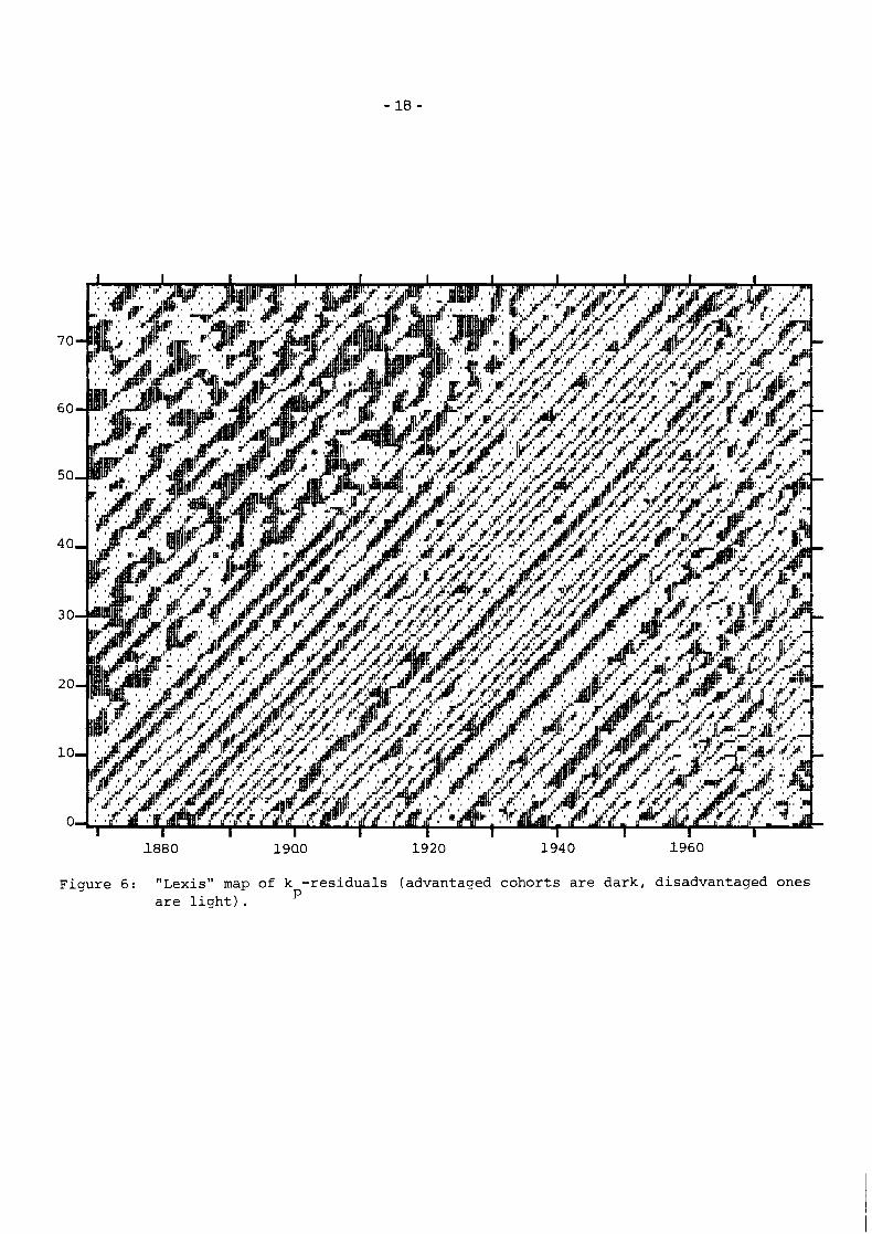
Figure 6: "Lexis" map of k -residuals (advantaged cohorts are dark, disadvantaged ones are light). P
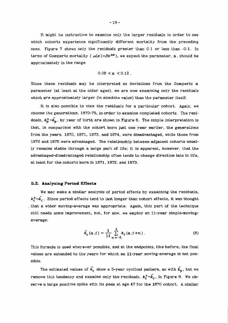
It might be instructive t o examine only t he l a r g e r residuals in o r d e r t o see
which cohorts experience significantly different mortality from the preceding
ones. Figure 7 shows only t h e residuals g r e a t e r than 0 .1 o r less than -0.1. In
terms of Gompertz mortality ( p ( x ) =BeaZ) , w e expect t h e parameter , a, should be
approximately in t h e range
Since these residuals may be interpreted as deviations f r o m the Gompertz a
parameter (a t least a t t h e older ages), w e are now examining only t he residuals
which are approximately l a r g e r (in absolute value) than the parameter itself.
I t is a lso possible to view the residuals for a par t icu la r cohort . Again, w e
choose t he generations, 1870-75, in o r d e r t o examine completed cohorts . The resi- n
duals, k;-kp, by yea r of b i r th are shown in Figure 8. The simple interpretat ion is
tha t , in comparison with t h e cohort born just one y e a r ea r l i e r , t he generations
from the years , 1870, 1871, 1873, and 1874, were disadvantaged, while those f r o m
1872 and 1875 were advantaged. The relationship between adjacent cohor t s usual-
ly remains s table through a la rge p a r t of life; i t i s apparen t , however, t ha t the
advantaged-disadvantaged relationship often tends t o change direction late in life,
at least fo r t h e cohor t s born in 1871, 1872, and 1873.
5.2. Analyzing Period Effects
W e may make a similar analysis of period effects by examining t h e residuals, n
k:-kc. Since period effects tend t o last longer than cohor t effects , i t was thought
t ha t a wider moving-average was appropriate . Again, this p a r t of t h e technique
sti l l needs some improvement, but, f o r now, w e employ an 11-year simple-moving-
average:
This formula is used wherever possible, and at the endpoints, l ike before , t h e final
values are extended t o t h e yea r s f o r which an 11-year moving-average is not pos-
sible. A
The estimated values of kc show a 5-year cyclical pa t te rn , as with ips but w e
remove this tendency and examine only t h e residuals, k: - iC , in Figure 9 . W e ob-
s e r v e a la rge positive spike with i ts peak at age 47 f o r t he 1870 cohort . A similar
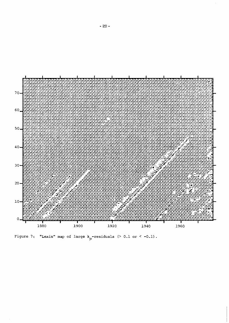
Figure 7: "Lexis" map of l a r g e k - r e s idua l s (> 0.1 o r < -0.1). p
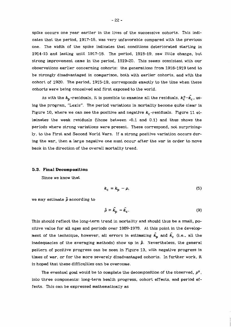
spike occurs one y e a r e a r l i e r in the lives of t he successive cohorts. This indi-
ca tes t ha t t he period, 1917-18, was very unfavorable compared with the previous
one. The width of t he spike indicates tha t conditions de te r iora ted s tar t ing in
1914-15 and lasting until 1917-18. The period, 1918-19, s a w l i t t le change, bu t
s t rong improvement came in t he period, 1919-20. This seems consistent with o u r
observations e a r l i e r concerning cohorts: t h e generations from 1916-1919 tend t o
be strongly disadvantaged in comparison, both with ea r l i e r cohorts , and with t h e
cohor t of 1920. The period, 1915-19, corresponds exactly t o t h e time when these
cohorts were being conceived and f i r s t exposed to t h e world.
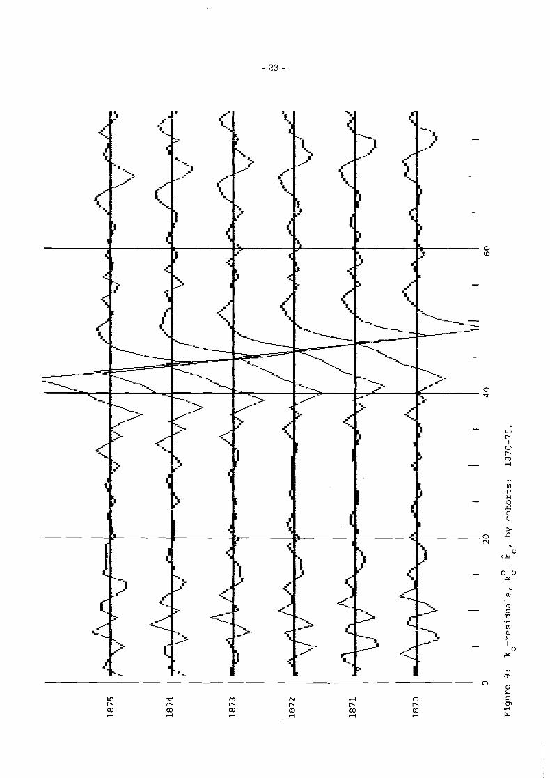
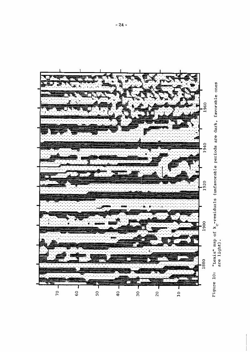
AS with t he $-residuals. i t i s possible t o examine all t h e residuals, k , ~ - & , us-
ing the program, "Lexis". The period variations in mortality become quite c l ea r in
Figure 10 , where w e can see the positive and negative kc-residuals. Figure 11 el-
iminates t he weak residuals (those between -0.1 and 0.1) and thus shows the
periods where s t rong variations were present . These correspond, not surprising-
ly, t o the Firs t and Second World Wars. If a s t rong positive variation occurs dur-
ing t he war, then a l a rge negative one must occu r a f t e r t he war in o r d e r t o move
back in t h e direction of t h e overall mortality t rend.
5.3. Final Decomposition
Since w e know t h a t
w e may estimate j according t o
This should r e f l ec t t h e long-term t rend in mortality and should thus be a small, po-
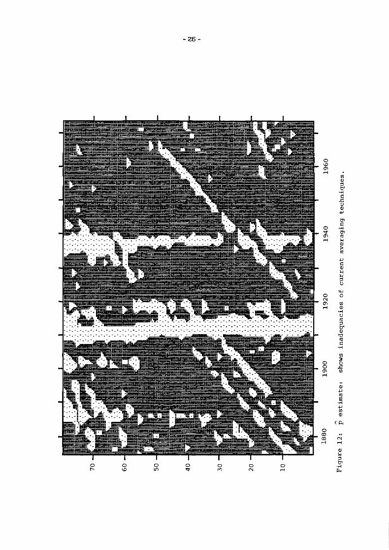
sitive value f o r all ages and periods ove r 1869-1978. A t th i s point in the develop-
ment of t he technique, however, a l l e r r o r s in estimating ip and ic (i.e.. all t h e
inadequacies of t h e averaging methods) show up in 5. Nevertheless, t h e general
pa t te rn of positive progress can be seen in Figure 13, with negative progress in
times of w a r , or f o r t h e more severely disadvantaged cohorts. In f u r t h e r work, i t
i s hoped tha t these difficulties can b e overcome.
The eventual goal would be to complete t he decomposition of t h e observed, p O ,
into t h r e e components: long-term health progress , cohor t effects, and period ef-
fects. This can b e expressed mathematically as
ffl 4 k 0 s 0 u
ffl d rd 3 "0 -4 ffl a k I u
X
[I) rl l-0 3 "0 -4 [I)
- - [I) -4
2 d -
= k; - k:
A A A
= kp - k c + (k; - kp) -(k: - i c )
=; + (k; - i p ) - (k; - i c )
= health progress + cohort effects + period effects . (10)
6. DISCUSSION
The technique, as i t now stands, appears t o be very useful in discerning con-
sistent mortality differences between adjacent bir th cohor t s and periods of time.
Several modifications suggest themselves which might extend t h e usefulness of t h e
technique.
By considering single-year cohorts, w e are limiting ourselves t o cohort
differences which must come from bir th . For instance, i t may be reasonable t o be-
lieve t ha t children who are born in a particularly unfavorable yea r could be s o
heavily affected by the lack of p rope r nutrition, poor living conditions, etc., while
still in t he womb o r during t h e f i r s t months of life, t ha t they could be disadvan-
taged through a long period compared t o t he cohort which w a s a l ready a y e a r old
at t h e time of t h e unfavorable conditions. That is t o say, t he difference in suscep-
tibility between age 0 and age 1 might truly be g rea t enough tha t cohor t differ-
ences could be observed.
On the o the r hand, w e might be interested in whether cohor t differentiation
can occur l a t e r in life as well. I t seems unreasonable, however, t o believe tha t
someone age 1 9 could somehow be more susceptible t o adverse conditions than
someone age 20 (an exception might be t he case of a one-year w a r where only
those 20 and ove r were involved in combat, but t he distinction would surely never
be s o clear) . I t does seem possible, though, tha t one five- o r ten-year age-group
might be more susceptible. Especially in t he case of war, t he age-groups who are
most heavily involved in fighting may subsequently be disadvantaged compared with
adjacent age-groups, who may have avoided act ive combat. Horiuchi (1983), in a
similar analysis, finds t ha t i t is t he 5-year cohort of men who were around age 15
at the end of t he two World Wars (in t he affected countries) who are the most disad-
vantaged l a t e r in l ife, although these men were too young t o have actually fought
in t h e wars.

Some work should also be done t o facilitate comparison of bir th cohorts born
more than one yea r apa r t . We might want t o know, f o r instance, which w a s t he
more disadvantaged cohort , 1917 o r 1919? W e need a means of measuring cumula-
t ive effects f o r cohorts. A simple average of t he kp-residuals f o r cohorts could be
made, and then a running total could be kept s o tha t all cohorts could be compared
on the same level. Even more instructive would be averages ove r different age
ranges; f o r example, before age 45 and a f t e r , in o r d e r t o observe whether cohort
variations change with age.
Other possible extensions of the model would include application t o o the r
kinds of demographic data. The prime candidate would seem t o be marriage r a t e s ;
o r , if the p rope r data were available, perhaps parity-specific ferti l i ty rates. The
essential requirement i s tha t t he age-structure of t he event change only slowly
over time. W e reca l l tha t this is what insures the stability of the kp and kc curves.
One necessary improvement which has already been noted is the question of
averages. There may exist more robust methods (running medians, f o r example) of
estimating $ and LC. The essential requirement is t ha t ip and dc should show ab-
solutely no signs of cohort o r period variation. A s noted, improving these two esti-
mates will automatically improve the estimate, i. If w e could then properly estimate 6, this would open up a whole new field of
research . A s a l ready observed, the crucial question in the traditional age-
period-cohort identification problem is tha t of how much of the long-term trend in
mortality should be at t r ibuted t o periods and how much t o cohorts. An accura te
estimate of this long-term t rend would be a useful s tar t ing point in any analysis.
Another extension of the technique which is called fo r is a means of estimating
the statistical significance of the cohort and period variations found. Very little
work has been done in this direction, but even a simple approach can b e quite in-
structive. For example, is i t significant tha t one cohort is advantaged compared
with another ove r a 10-year interval? Of course, if two cohorts a r e in a n exactly
equal relationship, the probability in any one period tha t one part icular cohort
would appea r advantaged ove r t he o ther one, due t o mere stochastic variation, is
one-half. The probability tha t t he same cohort would appea r advantaged ove r 10
successive periods, under t he hypothesis of equality, is
If we observe such a s tr ing of positive residuals, then, we may be fairly cer tain
tha t they a r e not due t o random fluctuations in mortality, but r a t h e r tha t they
represent r e a l differences (at least within the data!) between cohorts.
This las t parenthetical comment ref lects the continuing skepticism of the au-
t ho r concerning the possibility of systematic data e r r o r s which may have, in some
unknown way, c rea ted the observed results. In t he Italian data , especially f o r the
cohorts from 1862-1925 and f o r the periods before 1957, t he resul ts seem too reg-
u la r and show little evidence of stochastic variation. The plots of t he kp-residuals
f o r the cohorts , 1870-75, were more regular than could easily be believed. Some
of this may be due t o t he slight amount of smoothing tha t w a s applied t o the cohort
data, but this could not explain the high degree of regularity observed. I t also
seems r a t h e r mysterious tha t 1957 should mark both the end of the 5-year cyclical
pa t te rn and the beginning of a more random scheme of mortality (but one which
shows, nevertheless, a tendency toward cohort- and period-specific mortality vari-
ations). A s noted, 1957 corresponds, nei ther t o a change in demographic tech-
nique, nor t o a national census.
In support of the method is the f ac t tha t i t has also been successfully applied
t o French mortality da ta f o r the periods, 1899-1982, and none of t he same incon-
sistencies have been noted. The resul ts appear more random (in many ways similar
t o the l a t e r Italian data), but they sti l l show the usefulness of t he technique f o r ob-
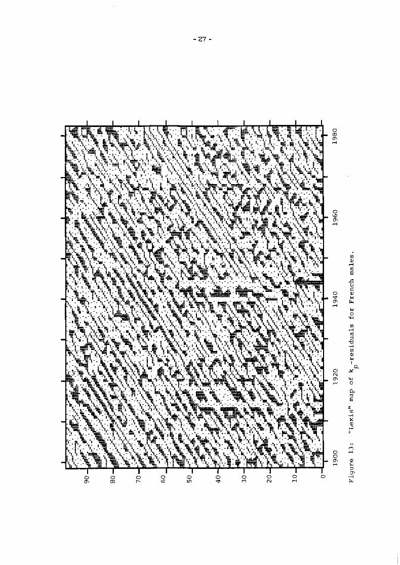
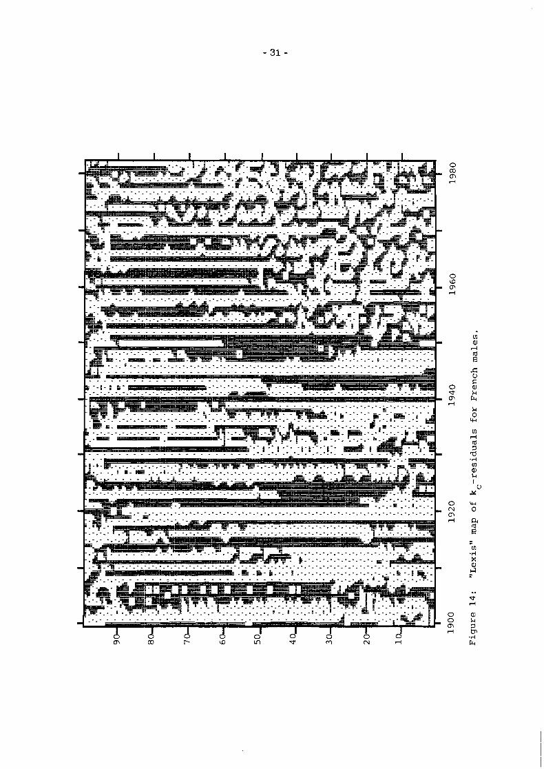
serving cohort and period variations. The graphs fo r French males which are com-
parable t o Figures 6 and 10 a r e shown in Figures 13 and 14. When w e examine the
kp-residuals in the cohort direction, the curves a r e not smooth, as in Figure 8 , but
more jagged, as w e might expect. Nevertheless, many cohorts show a c l ea r tenden-
cy t o be e i ther advantaged o r disadvantaged, as in the Italian data .
Furthermore, in support of t he Italian data itself, i t seems impossible tha t the
mortality f o r a cohor t could be systematically over- o r underestimated f o r the life
of t he cohort. Firs t , i t seems unreasonable tha t , in any one census, every o the r
age group would be overcounted while the o the r s would be undercounted. Second-
ly, censuses were conducted approximately every ten years (in 1881, 1891, 1901,
1911, 1921, 1931, 1951, 1961, 1971, and 1981), s o any systematic under- o r over-
count could not affect t he denominator in the qz rates f o r more than about 10
years . Lastly, beginning in 1928, all deaths were repor ted by single-year-of-age,
s o t h e r e is little possibility t ha t i t could be a problem with the numerators.
7 . CONCLUSIONS
It seems, then, tha t analyzing historical mortality data by single-year-of-age
and single-year-of-time may prove t o be a useful technique. There appea r t o be
cohort and period variations in mortality which often opera te on a time-scale of
one or two years , s o this f iner analysis seems to be required.
The technique of examining the derivatives on t h e mortality surface, log^,
proves t o be a very powerful one, both for discovering da ta inconsistencies and
for analyzing the da ta itself. I t is an excellent means of discerning cohor t and
period variations in mortality and may eventually be a successful means of decom-
posing observed mortality t rends into t h r ee components: t h e long-term. underly-
ing t rend , and the cohor t and period deviations f r o m tha t t rend.
More study is needed on the f iner points of applying t h e technique, on exten-
sion of t he technique t o allow g r e a t e r cohort and period comparison, on decompo-
sition of t h e long-term t rend of mortality a t various ages, on application of t he
technique to o t h e r types of demographic data , and, finally, on t he na ture of t he
data collection itself t o insure against data-related e r r o r s of analysis.
REFERENCES
Arthur, W .B . , and J . VJ. Vaupel (1984) Some general relationships in population dynamics. Popula t ion Index 50(2):214-26.
Caselli, G. , and R. Capocaccia (1985) Cohort and Early Debilitation Effects on Adult Mortality. Working Paper .
Caselli, G., J. Vaupel, and A. Yashin (1985) Mortali ty in Italy: Contours of a Cen- t u r y of Evolu t ion . CP-85-24. Laxenburg, Austria: International Institute f o r Applied Systems Analysis.
Coale, A.J., and E. Kisker (1985) Mortality crossovers: Reality or bad data? Prel- iminary d ra f t , presented at t h e annual meeting of t he Population Association of America, Boston, Massachussetts.
Horiuchi, S. (1983) The long-term impact of w a r on mortality: Old-age mortality of the Firs t World War surv ivors in the Federal Republic of Germany. Popula- t i o n Bul le t in of the United Nations, No. 15, pp. 80-92.
Horiuchi, S. , and A.J. Coale (1983) Age pa t te rns of mortality f o r older women: An analysis using the age-specific rate of mortality change with age. Presented at t he annual meeting of t he Population Association of America, Pit tsburgh, Pennsylvania.
Kermack, W.O., A.G. McKendrick, and P.L. McKinlay (1934) Death rates in Grea t Britain and Sweden: Some general regular i t ies and the i r significance. The Lancet, pp. 698-703.
McMillen, M.M., and C.B. Nam (1985) Mortality c rossovers by cause of death and race in t he U.S. in t h e 1970's. Presented at t h e biennial meeting of t h e Inter- national Union f o r t h e Scientific Study of Population, Florence, Italy.
Meindl, R.S. (1982) Components of longevity: Developmental and genetic responses t o differential childhood mortality. Social Science a n d Medicine 16:165-74.
Preston, S.H., and A.J. Coale (1982) Age s t ruc tu re , growth, a t t r i t ion, and acces- sion: a new synthesis. Popula t ion Index 48(2):217-59.
Preston, S.H., and E. Van d e Walle (1978) Urban French mortality in t he nineteenth century. Popula t ion S tud i e s 32(2):275-97.
Vaupel, J.W., G . Manton, and E. Stal lard (1979) The impact of heterogeneity in indi- vidual f ra i l ty on the dynamics of mortality. D?mography 16(3):439-54.
Vaupel, J.W., and A.I. Yashin (1985) The deviant dynamics of death in heterogene- ous populations. Sociological Methodology 2985, pp. 179-211.