1

Identification of Catalytic Converter Kinetic Model Using a Genetic Algorithm Approach

G.N. Pontikakis and A.M. Stamatelos*

Mechanical & Industrial Engineering Department

University of Thessaly

Abstract The need to deliver fast-in-market and right-first-time ultra low emitting vehicles at a reasonable cost is driving the automotive industry to invest significant manpower in the computer-aided design and optimization of exhaust aftertreatment systems.

To serve the above goals, an already developed engineering model for the three-way catalytic converter is linked with a genetic algorithm optimization procedure, for fast and accurate estimation of the set of tunable kinetic parameters that describe the chemical behavior of each specific washcoat formulation. The genetic algorithm-based optimization procedure utilizes a purpose-designed performance measure that allows an objective assessment of model prediction accuracy against a set of experimental data that represent the behavior of the specific washcoat formulation over a typical test procedure.

The identification methodology is tested on a characteristic case study, and the best fit parameters produced demonstrate a high accuracy in matching typical test data. The results are far more accurate than those that may be obtained by manual or gradient-based tuning of the parameters.

Moreover, the set of parameters identified by the GA methodology, is proven to describe in a valid way the chemical kinetic behavior of the specific catalyst.

The parameter estimation methodology developed, fits in an integrated computer aided engineering methodology assisting the design optimization of catalytic exhaust systems, that extends all the way through from the model development to parameter estimation, and quality assurance of test data.

* corresponding author, Laboratory of Thermodynamics & Thermal Engines, Mechanical & Industrial Engineering Department, University of Thessaly, 383 34 Volos, Greece. Tel: +30-24210-74067, Fax: +30-24210-74050, e-mail: stam@uth.gr

2

Introduction The catalytic converter has been in use for the past 30 years as an efficient and economic solution for the legislated reduction of pollutants emitted by passenger car engines. Nowadays, emission legislation becomes gradually stricter, in an effort to control air pollution especially in urban areas. This trend has led to the development of high efficiency exhaust aftertreatment systems, which involve the careful optimization and operation control of the engine, piping and catalytic converter for each application. The development of such systems is a complex task that is supported by catalytic converter modeling tools. Modern modeling methodologies have demonstrated their capacity to be successfully incorporated in the process of exhaust aftertreatment systems design [1,2,3,4,5].

Among the plethora of catalytic converter models that have appeared in the literature, engineering models with reduced reactions schemes and semi-empirical rate expressions appear to be better suited to the requirements and constraints of the automotive engineer [6]. Such models are proven able to match the accuracy levels and scope of the data of legislated driving cycle tests, and provide the engineer with reliable, fast and versatile tools that may significantly decrease the cost and development time of new exhaust lines.

Reduced reaction scheme models employ a limited number of phenomenological reactions that contain only initial reactants and final products instead of elementary reactions on the catalyst active sites. The complexity and details of the reaction path is lumped into the kinetic rate expressions of these models, hence called lumped-parameter models. Rate expressions usually follow the Langmuir–Hinselwood formalism, modified by empirical terms. Generally, the form of the rate expressions of such models for the reaction between two species a and b is:

( ),...,,...;, 21

/

KKccGccAer

ba

baRTE−

= (1)

Thus, the Langmuir–Hinselwood rate expressions determine an exponential (Arrhenius type) dependence on temperature while G is an inhibition term, a function of temperature and concentrations c of various species that may inhibit the reaction.

In the above expression, factors A and E (the pre-exponential factor or frequency factor and the activation energy) as well as factors K included in the inhibition term G are considered as fitting (tunable) parameters. The effect of all phenomena not included explicitly into the model is lumped in these terms. Therefore, their values are dependent on the chemical composition of the catalyst’s washcoat and must be estimated by fitting the model to a set of experimental data, which represent the behavior of the catalyst in typical operating cycles.

The identification of the model’s tunable parameters is commonly referred to as model tuning. The applicability of the lumped parameter models is significantly affected by the successful identification of the tunable parameters. Once an accurate parameter identification is succeded, the model may be used subsequently for the prediction of the catalytic converter efficiency for different geometrical and design characteristics or under different operation conditions.

Traditionally, fitting of lumped parameter catalytic converter models was accomplished manually, a process which is highly empirical, requires experience and does not guarantee the success of the undertaking. To circumvent these drawbacks, several efforts have appeared towards a systematic methodology for model tuning. All of them are based on the transformation of the tuning problem into an optimization problem, where a quantity that indicates goodness-of-fit is optimized for the tunable parameters of the model. The goodness-of-fit quantity may be viewed as a performance measure of the model, since it indicates the performance of the model compared to the experimental data.

Montreuil et al. [7] were the first to present a systematic attempt to tune their steady state three-way catalytic converter model, using a conjugate gradients optimization procedure. Dubien and Schweich [8] presented a conceptually similar methodology to determine the kinetics of simple

3

rate expressions from light-off experiments, employing the downhill simplex method. Pontikakis and Stamatelos [9] used the conjugate-gradients technique to determine kinetic parameters of a transient three-way catalytic converter model from driving cycle tests. Glielmo and Santini [10] presented a simplified three-way catalytic converter model oriented to the design and test of warm-up control strategies and tuned it using a genetic algorithm. All of the above efforts used a performance measure based on the least-squares error [11] between measured and computed results. The work of Glielmo and Santini must be distinguished, though, because it is the only one that uses a multi-objective optimization procedure for the identification of the model. The genetic algorithm has the potential to avoid local optima in the optimization space and thus fit the model to the experimental data with higher accuracy.

The combination of a lumped-parameters catalytic converter model with an optimization procedure for the identification of the model’s parameters is only a first step towards a complete, computer-aided methodology for catalytic converter design and optimization, which is under continuous development at the authors’ Lab during the last decade. The complete methodology is based on the following four-fold framework:

— Catalytic converter model and software package based on tunable LH kinetics approach

— Kinetic parameter estimation software based on a properly adapted optimization procedure

— Emissions measurements quality assurance methodology and software

— Design and implementation of critical experiments to improve understanding and modeling of catalytic converters

This work is a continuation of the work presented in [9] and addresses the interaction of the first two of the above issues. It is based on the CATRAN three-way catalytic converter (3WCC) model, which is already developed and has been validated against a number of real world case studies [12]. The performance measure and the optimization algorithm of the procedure are updated, in an attempt to approach the problem of computer-aided identification of the kinetic model more systematically. Specifically, a performance measure is first formulated that is suited to the problem of catalytic converter model tuning in driving cycle tests. Then, a purpose – designed genetic algorithm is used to extract a set of tunable parameters that optimizes the performance measure to obtain a good fit of the model to the experimental data.

Model description The catalytic converter model used in this study is briefly described below. The model’s underlying concept is the minimization of degrees of freedom and the elimination of any superfluous complexity in general. A more detailed description of the model and its design concept is given in [6].

The prevailing physical phenomena that occur in the catalytic converter are heat and mass transfer in both gaseous and solid phases. They are described by a system of balance equations, which is summarized in Table 1. The model features:

— Transient, one-dimensional heat transfer calculations for the solid phase of the converter.

— Quasi-steady, one-dimensional calculations of temperature and concentration axial distributions for the gaseous phase

4

— Simplified reaction scheme featuring a minimum set of Langmuir-Hinselwood-type reduction–oxidation (redox) reactions and an oxygen storage submodel for three-way catalytic converter washcoats.

The one-dimensional approximation of the converter neglects any non-uniformity of inlet flow profiles. Heat transfer in the solid phase involves a fully transient calculation. Nevertheless, quasi-steady heat and mass balances are employed for the gas-phase, since the heat and mass accumulation terms in the gas phase are neglected, which is a realistic assumption [13,14]. The washcoat is approximated with a solid–gas interface, where all reactions occur. That is, diffusion effects are neglected completely, and it is assumed that all catalytically active cites are directly available to gaseous-phase species at this solid–gas interface [15,16].

For the formulation of the reaction scheme, the three-way catalytic converter will be considered, which is designed for spark-ignition engines exhaust. There are two types of heterogeneous catalytic reactions that occur in the 3WCC washcoat: Reduction–oxidation (redox) reactions and oxygen storage reactions. The complete reaction scheme of the model, along with the rate expression for each reaction, is summarized in Table 2. Below, we examine the features of the reaction scheme in some more detail.

Redox reactions take place on the precious metal loading of the washcoat (a combination of Pt, Pd, and Rh, depending on the formulation) and involve oxidation of CO, H2 and the complex mixture of the hydrocarbons (HC) of the exhaust gas, as well as reduction of nitrous oxides (NOx) to N2. Oxygen storage reactions proceed on the Ceria component of the washcoat, where 3-valent ceria oxide (Ce2O3) is oxidized by O2 and NO to its 4-valent counterpart (CeO2). In its turn, CeO2 is reduced by CO and hydrocarbons to Ce2O3.

In the present model, the oxidation reactions rates of CO and hydrocarbons are based on the expressions by Voltz et al. [17], which were originally developed for a Pt oxidation catalyst but, interestingly enough, they are still successful, with little variation, in describing the performance of Pt:Rh, Pd, Pd:Rh and even tri-metal catalyst washcoats.

In practice, analyzers measure only the total hydrocarbon content of the exhaust gas and make no distinction of the separate hydrocarbon species. Therefore, for modeling purposes, the total hydrocarbon content of the exhaust gas is divided into two broad categories: easily oxidizing hydrocarbons (“fast” HC), and a less-easily oxidizing hydrocarbons (“slow” HC). Throughout this work, it is assumed that the exhaust hydrocarbon consisted of 85% “fast” HC and 15% “slow” HC. This is a rough approximation introduced in lack of more accurate data but, according to our experience, it gives satisfactory result. Both fast and slow hydrocarbons are represented as CH1.8, since average ratio of hydrogen to carbon atoms in the exhaust gas is 1.8. Thus, the two hydrocarbons are distinguished in the model only by the difference in the kinetic parameters.

For the reaction between CO and NO we employ a simple Arrhenius-type reaction rate. Finally, hydrogen oxidation is also included in the model; the Voltz rate expression is used for H2 oxidation as well.

Oxygen storage is taken into account by the model by four reactions for Ce2O3 oxidation by O2 and NO, and CeO2 reduction by CO and HC. The model uses the auxiliary quantity ψ to express the fractional extent of oxidation of the oxygen storage component. It is defined as:

322

2

OCe moles2CeO molesCeO moles×+

=ψ (2)

The extent of oxidation ψ is continuously changing during transient converter operation. Its value is affected by the relative reaction rates of reactions 6–9. The rates of reactions are expected to be linear functions of ψ for CeO2 reduction and (1−ψ) for Ce2O3 oxidation. The rate of variation of ψ is the difference between the rate that Ce2O3 is oxidized and reduced:

5

capcap Ψr

Ψrr

dtd 8109 +

+−=

ψ (3)

The above equation is solved analytically for ψ at each node along the catalyst channels. The quantity Ψcap is the total oxygen storage capacity and its value may be estimated by the content of Ceria in the washcoat. In this work, the value of Ψcap is approximated to 600 mol O2/mol Ce.

Tuning procedure

General

The reaction rate expressions introduce into the catalytic converter model a set of parameters that have to be estimated with reference to a set of experimental data. In the present model, the set of tunable parameters is formed by the pre-exponential factors Ak that are included in the reaction rates rk. Our objective is to fit them against experimental data from a routine driving cycle test.

In concept, the activation energy Ek of each reaction and the set of terms Ki, included in the Voltz inhibition term G, may also be considered as tunable parameters; we do not attempt to tune them though. The activation energy of each reaction is approximately known from previous experience and their variation over different washcoat formulations is not significant. Furthermore, the Voltz inhibition factor without modification in its term has been found to consistently give satisfactory results for a wide range of washcoats. Besides, any attempt to tune the activation energy or the inhibition term of any reaction would require data of increased accuracy, which is not provided by driving cycle tests and may only be feasible with specialized experiments.

Additionally, the kinetic constants of H2 oxidation are also not tuned in this work. The H2 content of the exhaust gas is low and is not known accurately because it may not be measured and has to be implicitly computed [18]. Therefore, we fix their values as equal to the values of CO oxidation constants. This is a practice suggested from previous experience. Thus, there are nine tunable parameters in total, one for each reaction except of the reaction of H2.

Since the problem of model tuning is a parameter-fitting problem, it may be tackled as an optimization problem. This involves the development of two components:

1. A performance measure, which qualitatively assesses the goodness-of-fit of the model for each possible set of parameter values.

2. An optimization procedure, which finds a set of tunable parameters giving an optimum value for the performance measure, i.e. yields in modeling results that are as close to the measured results as possible.

The most usual performance measure used in the bibliography is based on the least-squares error between measured and computed instantaneous concentrations of pollutants at the converter’s outlet. Here, we modify a new performance measure that is more beneficial for optimization purposes and may also be used independently as an objective, generic measure to compare the performance of different models.

The performance measure was optimized using a genetic algorithm, because previous experience has shown that the problem of model parameter estimation is multimodal, and the genetic algorithm is a powerful technique for multimodal optimization. The genetic algorithm was properly adapted to the problem at hand. The details of performance measure and genetic algorithm formulation are presented below.

6

Formulation of the performance measure

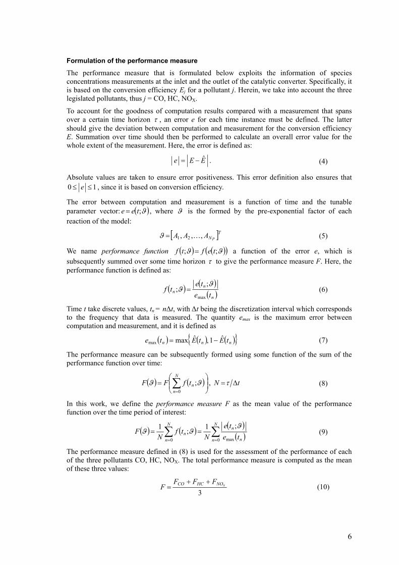
The performance measure that is formulated below exploits the information of species concentrations measurements at the inlet and the outlet of the catalytic converter. Specifically, it is based on the conversion efficiency Ej for a pollutant j. Herein, we take into account the three legislated pollutants, thus j = CO, HC, NOX.

To account for the goodness of computation results compared with a measurement that spans over a certain time horizon τ , an error e for each time instance must be defined. The latter should give the deviation between computation and measurement for the conversion efficiency E. Summation over time should then be performed to calculate an overall error value for the whole extent of the measurement. Here, the error is defined as:

EEe ˆ−= . (4)

Absolute values are taken to ensure error positiveness. This error definition also ensures that 10 ≤≤ e , since it is based on conversion efficiency.

The error between computation and measurement is a function of time and the tunable parameter vector: ( )ϑ;tee = , where ϑ is the formed by the pre-exponential factor of each reaction of the model:

[ ]TNPAAA ,,, 21 K=ϑ (5)

We name performance function ( ) ( )( )ϑϑ ;; teftf = a function of the error e, which is subsequently summed over some time horizon τ to give the performance measure F. Here, the performance function is defined as:

( ) ( )( )n

nn te

tetf

max

;;

ϑϑ = (6)

Time t take discrete values, tn = n∆t, with ∆t being the discretization interval which corresponds to the frequency that data is measured. The quantity emax is the maximum error between computation and measurement, and it is defined as

( ) ( ) ( ){ }nnn tEtEte ˆ1,ˆmaxmax −= (7)

The performance measure can be subsequently formed using some function of the sum of the performance function over time:

( ) ( )

= ∑

=

N

nntfFF

0

;ϑϑ , tN ∆=τ (8)

In this work, we define the performance measure F as the mean value of the performance function over the time period of interest:

( ) ( ) ( )( )∑∑

==

==N

n n

nN

nn te

teN

tfN

F0 max0

;1;1 ϑϑϑ (9)

The performance measure defined in (8) is used for the assessment of the performance of each of the three pollutants CO, HC, NOX. The total performance measure is computed as the mean of these three values:

3xNOHCCO FFF

F++

= (10)

7

The above performance measure presents advantageous features compared to the classical least-squares performance measure:

— It ranges between two, previously known, finite extreme values. Extremes correspond to zero and maximum deviation between calculation and experiment.

— The extrema of the performance measure are the same for all physical quantities that may be used and all different measurements where the performance measure may be applied. That is, the performance measure is normalized so that its extrema do not depend on the either the measured quantities or the experimental protocol.

It should be noted here that, because of the above properties, this performance measure may be used as a general measure to compare the model’s performance under different cases studies, or compare alternative models for a single case study. That is, it is a generic quantitative measure to assess the model’s performance. This should be contrasted to the usual practice for model assessment, which is simply based on inspection. Although a visualization procedure is necessary to gain insight to the model’s results, it is a subjective criterion. A least-squares performance measure, on the other hand, depends on the measurement at hand and is not helpful for comparison purposes. A normalized performance measure such as the one defined above eliminates this problem and should provide more insight to model assessment.

From the optimization point of view, normalization of the performance measure is required because the total performance measure F is computed as the mean of FCO, FHC and FNOx. If each of the individual performance measures were not normalized by definition, they would take values of different points of magnitude. Then, arbitrary scaling factors (weights) would be necessary before taking the average to compute F. With the current performance measure definition, this is avoided.

Optimization procedure

Having defined the performance measure for the model, the problem of tunable parameter estimation reduces in finding a tunable parameter vector ϑ that minimizes F. Owing to the multimodal character of the problem, a genetic algorithm has been employed for the task. Since genetic algorithms are maximization procedures, the problem is converted into a maximization problem for F', defined as: F'=1−F.

Summarizing the above, the mission of the genetic algorithm is to solve the following problem:

Maximize ( ) ( )( )

( )∑ ∑= =

=−=′xNOHCCOj

N

n nj

nj

tete

NFF

,, 0 max,

;311

ϑϑϑ (11)

This is a constraint maximization problem, since the components of vector ϑ are allowed to vary between two extreme values, i.e. max,min, iii ϑϑϑ ≤≤ .

The genetic algorithm is a kind of artificial evolution, where a population of solutions evolves similarly to the nature’s paradigm: Individual solutions are born, reproduce, are mutated and die in a stochastic fashion that is nevertheless biased in favor of the most fit individuals [19]. The implementation of the algorithm that has been developed in this work takes the following steps:

1. Initialization. A set of points in the optimization space is chosen at random. This is the initial population of the genetic algorithm, with each point (each vector of tunable parameters) corresponding to an individual of the population.

2. Fitness calculation. The fitness of each individual in the population is computed using (11). It should be noticed that fitness calculation requires that the model be called for each individual, i.e. as many times as the population size.

8

3. Selection. Random pairs of individuals are subject to tournament, that is, mutual comparison of their fitnesses [20]. Tournament winners are promoted for recombination.

4. Recombination (mating). The simulated binary crossover (SBX) operator [21] is applied to the couples of individuals that are selected for recombination (parents). The resulting chromosomes are inserted in the children population.

5. Mutation. A small part of the population is randomly mutated, i.e. random parameters of the chromosomes change value in a random fashion [22].

6. Original parent population is discarded; children population becomes parent population.

7. Steps 3 to 6 are repeated for a fixed number of generations or until an acceptably fit individual has been produced.

Genetic algorithms are not black-box optimization techniques. On the contrary, a genetic algorithm should be adapted by the user to the target problem [20]. There are a number of design decisions and parameters that influence the operation, efficiency and speed of the genetic algorithm. The present implementation is summarized in Table 3. The genetic algorithm is a real-coded genetic algorithm and uses the simulated binary crossover (SBX) [21] for the mating and recombination of individuals.

The SBX operator works directly on the real-parameter vector that represents each individual, thus eliminating the need for a real-to-binary encoding-decoding required in binary encoded genetic algorithm. SBX operator also works on arbitrary precision, which should be contrasted to the finite precision of binary encodings.

The randomized nature of the genetic algorithm enables it to avoid local extrema of the parameter space and converge towards the optimum or a near-optimum solution. It should be noted, though, that this feature does not guarantee convergence to the global optimum. This behavior is common to all multimodal optimization techniques and not a specific genetic algorithm characteristic.

Application case study The validity of the approach that is described above is assessed in a real-world application case. Manual tuning of the model is originally performed, and the results are subsequently compared with the identification results produced by the genetic algorithm. It is found that the genetic algorithm manages to find a set of tunable parameters that fits the experimental data with much higher accuracy compared to the manual efforts. In order to check the usability of the GA-tuned model, we apply it to a second set of driving cycle data, obtained with a catalyst with significantly reduced size. It is found that the model is able to predict the efficiency of the second catalyst successfully.

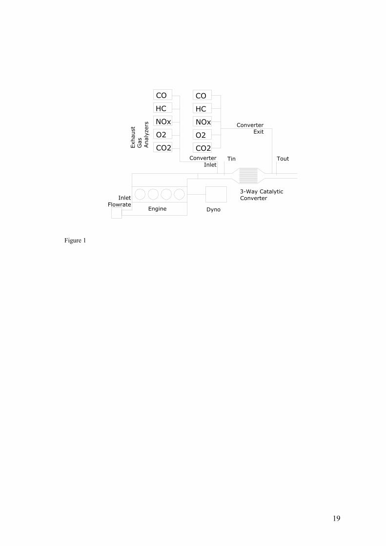
Specifically, in this application example, we are going to employ a set of measurements of emissions upstream and downstream a Pt:Rh (5:1) catalyst installed on a 1.8 l gasoline engine, that has followed a simulated New European Driving Cycle test on the computer controlled engine bench. The catalytic converter has a circular cross-section of 127 mm diameter and it is consisted of 2 beds with a total length of 203 mm. CO, HC NOx, O2 and CO2 analyzers measure the exhaust gas content upstream and downstream the catalyst. Figure 1 presents an overview of the emissions measurements setup.

Figure 2 presents a summary of the measured results after preprocessing with the data consistence and error checking routines [23]. Evidently, the catalytic converter light-off occurs at about 50 s after the beginning of the measurement. After light-off, and up to about 800 s,

9

emissions are almost zeroed. The first 800 s correspond to the urban phase of the driving cycle. During this phase, only few emission breakthroughs occur. Comparatively more pollutants are emitted in the period from 800 to 1180 s (which corresponds to the extra-urban phase of the NEDC), because of the higher space velocity of the exhaust gas.

It is important to note that, because of the very low emission standards, it does not suffice to predict the light-off point of the catalyst. Increased accuracy is demanded during the whole extent of the cycle test. The low levels of concentrations at the catalyst exit, compared to the corresponding concentrations at the inlet, further complicate the undertaking. Its success is thus heavily dependent on both the careful model formulation and the accurate tunable parameter identification.

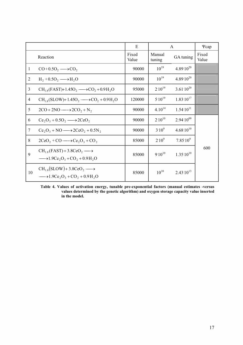
Proceeding to the model identification, we present in Table 4: (a) the set of kinetics parameters of the model and (b) their values tuned manually and by the genetic algorithm.

In principle, the kinetic parameters are 21 in total: One parameter for the oxygen storage capacity, and 10 couples of parameters (A and E) for the 10 reactions incorporated in the reaction scheme.

As previously discussed, not all kinetic parameters are tuned. The activation energies are more or less known from previous experience [24]. They could be varied a little, but this is not necessary since the rate depends on both A and E and any small difference can be compensated by respective modification of A. The oxygen storage capacity is also not tuned, since its approximate magnitude is estimated based on the washcoat composition (Ce, Zr) [25], and is also checked by characteristic runs of the code. Finally, the H2 oxidation kinetics is assumed to be approximately equal to that of CO oxidation.

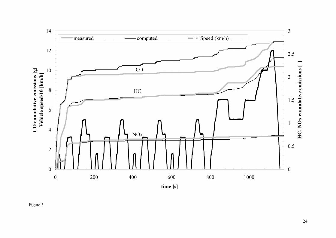
Thus, we are left with nine pre-exponential factors to be tuned: 4 reactions of gaseous phase species on the Pt surface, and another 5 reactions on the Ceria – Zirconia components of the washcoat. The manual tuning that was initially performed gives the results that are illustrated in Figures 3 and 4. Manual tuning was performed following a trial-and-error procedure and was mainly aided by previous experience with similar catalysts. Figure 3 gives the cumulative emissions for all pollutants. Although the computed total mass of pollutants matches the measurements, Figure 3 imply low accuracy for the prediction of instantaneous emissions, especially for the CO. This is better shown in Figure 4, where the computed instantaneous CO concentrations at the outlet can only qualitatively fit the measurement.

The model’s accuracy concerning instantaneous emissions is significantly improved when the model is fitted using the genetic algorithm. The comparison of computed vs. measured cumulative emissions is illustrated in Figure 5. The form of the curves for all three pollutants matches the measured data much more closely, which indicates that the instantaneous emissions of the model are fitted with good accuracy. The computed and measured instantaneous emissions for CO, HC and NOx are compared in Figures 6, 7 and 8 respectively.

It must be noted that the fit of the model is more successful for the CO and HC curves than for the NOx curve. This is mainly attributed to the Voltz inhibition term for the CO and HC oxidation reactions. On the contrary, no appropriate inhibition term has been extracted for the reactions that involve NOx. Furthermore, comparing the fit for CO and HC curves, we may readily find that HC fit is inferior. This is expected since the complicated mixture of hydrocarbons contained in the exhaust gas is approximated by only two components, a “fast” and a “slow” hydrocarbon. Bearing in mind that this is a very gross approximation, the model may be considered fairly satisfactory.

The evolution of the genetic algorithm population of solutions is indicative of the problem difficulty and explains the limited success of manual tuning or tuning that uses gradient-based methods. To illustrate the evolution process, a graph of the evolution of maximum and average fitness of the population is presented in Figure 9. The genetic algorithm quickly improves the maximum performance measure solution at the beginning of the run. Then, evolution is slower

10

and after some point, it completely stalls. This indicates that the genetic algorithm population has converged to a specific attraction basin of the optimization space and not much improvement may be achieved. At this point, the algorithm is stopped. The specific computation required about 72 hours on a 2.4 GHz Pentium 4 computer.

It may be noted that the absolute value of the performance measure does not vary much during the GA run. This is a property of the performance measure formulation but also indicates the multi-modality of the problem, since it appears that many combinations of kinetic parameters leads to the same overall performance of the model.

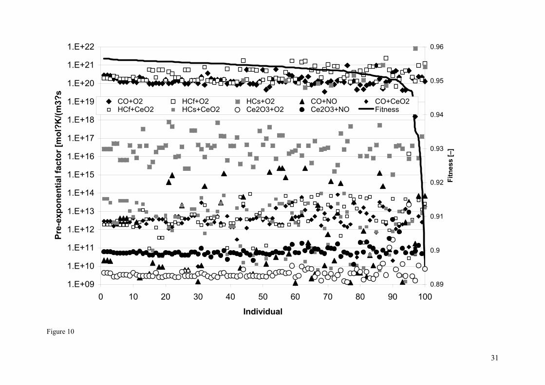
The spread of individuals in the 20th, the 45th and the last (135th) generation is given in Figures 10, 11 and 12 respectively. The individuals are sorted in descending order according to their performance measure.

Figure 10 visualizes the spread of the kinetic parameters in the population of the genetic algorithm near the beginning of the procedure. The kinetic parameters are allowed to vary in certain intervals that are induced based on previous experience and are consistent with their physical role in the respective reactions. The different kinetic parameters pertaining to reactions that occur on the three distinct catalytic components of the washcoat (in our example, Pt, Rh and Ce) fall in three distinct intervals.

Figure 11 gives the spread of individual solutions in the 45th generation of the population. Apparently, the population has started converging for the pre-exponential factors of some reactions. This indicates that the kinetics of these reactions influence the quality of the model fit (and thus the performance measure value) much more significantly than the rest of the reactions.

Figure 12 presents the last population of the GA run. It is evident that the parameters for the oxidation of “slow” hydrocarbons with oxygen on Pt or with stored oxygen do not converge, whereas the rest of the parameters show clear signs of convergence. This could be attributed to the fact that the “slow” hydrocarbons are only 15% of the total hydrocarbon content and thus influence the total hydrocarbon efficiency of the catalyst much less compared to the “fast” hydrocarbons. The same absence of convergence is noticed for the kinetics of CO+NO reaction, whereas the complementary reaction of Ceria + NO shows clear signs of convergence. This fact hints to a lack of sensitivity of the model regarding the above three reactions. One should not deduce at this early investigation point, that these reactions are less important than the rest to the model’s accuracy and predictive ability. Experience shows that further reduction of the number of reactions leads to an observable deterioration of the model fitting ability.

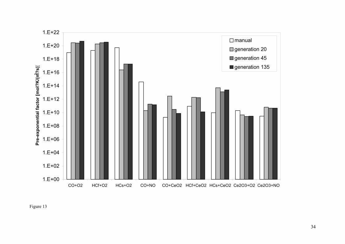
For comparison purposes, the best set of kinetic parameters values derived at the three characteristic generations of the GA evolution are presented, along with the manually derived set, in Figure 13.

The above discussion should make apparent that the parameter identification methodology developed gives significant feedback also to the reaction modeling. This is a subject of continuing investigation.

As a next step in the evaluation of the parameter identification methodology, the kinetic parameters derived by the genetic algorithm for the full scale converter, are applied in the prediction of the behavior of a reduced size converter with the same washcoat formulation and loading. The model’s prediction is checked against experimental results obtained with a cylindrical converter of 120 mm diameter and 60 mm length. The results are presented in Figure 14 in the form of cumulative CO, HC and NOx emissions.

The results are indicative of the model’s predictive ability of the 1D model for typical quality test data. As a typical example of the model’s performance, the computed instantaneous HC emissions are compared to the experimental ones in Figure 15. Evidently, the model prediction continues to be acceptably close to the experimental data, both qualitatively and quantitatively, which further supports the validity of the kinetic model approach.

11

Conclusions • A genetic algorithm methodology was developed for the identification of the kinetic

submodel of a previously developed 3WCC model. This is a one-dimensional model for the heat and mass transfer in the catalytic converter that features a reduced kinetics scheme.

• This scheme involves rate expressions which contain a limited number of apparent kinetic parameters that may be viewed as fitting parameters. Their values are identified in order to fit a set of experimental data that represent the behaviour of the specific washcoat formulation over a typical test procedure.

• In this paper, a complete identification methodology for the above problem is formulated in two steps. First, a performance measure is defined that is suitable for the assessment of the model’s performance in fitting the data. Second, a genetic algorithm is employed that uses the performance measure as an objective function. The genetic algorithm searches the parameter space to find the optimal set of parameters producing the best fit to the data.

• The identification methodology is tested on a characteristic case study, and the best fit parameters produced demonstrate a high accuracy in matching the test data describing the behavior of a specific catalyst installed on a 1.8 l passenger car engine tested according to the NEDC procedure. The results are far more accurate than those that may be obtained by manual or gradient-based tuning of the parameters, because the search space is highly multimodal, which causes non-stochastic search procedures to get trapped to local optima.

• Moreover, the set of parameters identified by the GA methodology, is proven to describe in a valid way the chemical kinetic behavior of the specific catalyst. This is proven by an application of the specific set of kinetic parameters, to predict the behavior of a reduced size converter with the same catalyst formulation. The prediction accuracy is remarkable if one takes into account the statistical variation of the performance of such a complex system.

• The parameter estimation methodology developed, is completing a previously developed systematic computer aided engineering methodology assisting the design optimization of catalytic exhaust systems, that extends all the way through from the model development to parameter estimation, and quality assurance of test data.

12

List of Symbols aj,k stoichiometric coefficient of species j in reaction k A Pre-exponential factor of reaction rate expression, [mol·K/(m3s)] c Species concentration, [–] cp Specific heat capacity, [J/(kg·K)] e Error between computeration and experiment, [–] E 1. Activation energy of reaction rate expression, [J] 2. Conversion efficiency, [–] f performance function, [–] F performance measure, [–] G Inhibition term (Table 2), [K]

H∆ Molar heat of reaction, [J/mol] h Convection coefficient, [W/(m2s)] k Thermal conductivity, [W/(m·K)] km mass transfer coefficient, [m/s] K Inhibition term (Table 2), [–] m& Exhaust gas mass flow rate, [kg/s] M Molecular mass, [kg/mol] Qamb Heat transferred between converter and ambient air, [J/(m3·s)] r Rate of reaction, [mol/m3s] Rg Universal gas constant, [8.314 J/(mol·K)] R Rate of species production/depletion per unit reactor volume, [mol/(m3s)] S Geometric surface area per unit reactor volume, [m2/m3] t Time, [s] T Temperature, [K] uz Exhaust gas velocity, [m/s] z Distance from the monolith inlet, [m]

Greek Letters

γ Catalytic surface area per unit washcoat volume, [m2/m3]

δ washcoat thickness, [m] ε emissivity factor (radiation), [m−1] ϑ tunable parameters vector ρ density, [kg/m3]

σ Stefan–Boltzmann constant, [W/(m2·T4)] τ duration of an experiment, [s] ψ fractional extent of the oxygen storage component, [–]

capΨ washcoat capacity of the oxygen storage component, [mol/m3]

Subscripts amb ambient g gas i parameter index

13

j species index k reaction index n time index in inlet s 1. solid, 2. solid–gas interface z axial direction

14

List of Tables

Model equations Tunable parameters

Gas phase (channel)

( ) ( ) ( )( )zczcSkz

zcu jsjjmg

jzg ,, −=

∂∂

ρρ —

Mas

s bal

ance

s

Solid phase (washcoat)

( ) jsjjjmg

g RccSkM

=− ,,ρ

—

Gas phase (channel)

( ) ( ) ( )( )zTzThSz

zTuc gs

gzps −=

∂

∂ρ —

Hea

t bal

ance

s

Solid phase (washcoat)

( ) ( ) amb

N

kkksg

szs

ssps QrHTThS

zTk

tTc

R

+∆−+−+∂∂

=∂

∂ ∑=1

2

2

,,ρ —

Reaction rates ( )∑=

=RN

kkkjj raSR

1,γδ . (rk is defined for each

reaction in Table 2) Ak

k=1…9

Boundary conditions

( ) ( )44ambsambsambamb TTTThQ −+−= εσ

( ) ( )( ) ( )( ) ( )tmztm

tTztTtcztc

in

ingg

injj

&& ==

==

==

0,0,0,

,

,

j = CO, O2, H2, HCfast, HCslow, NOx, N2.

—

Table 1. Model equations and tunable parameters

15

Reaction Rate expression

Oxidation reactions

1 22 CO0.5O+CO → G

cceAr OCO

TRE g2

11

1

−

=

2 OH0.5O+H 222 → G

cceAr OH

TRE g22

22

2

−

=

3 OH9.0COO45.1(FAST)CH 2221.8 +→+ G

cceAr OHCfast

TRE g2

33

3

−

=

4 OH9.0COO45.1(FAST)CH 2221.8 +→+ G

cceAr OHCslow

TRE g2

44

4

−

=

NO reduction

5 22 N2CO2NO2CO +→+ NOCOTRE cceAr g5

55−=

Oxygen storage

6 2232 2CeOO5.0OCe →+ ( )ψ−= − 12

666 O

TRE ceAr g

7 2232 N5.02CeONOOCe +→+ ( )ψ−= − 1777 NO

TRE ceAr g

8 2322 CΟCeCΟ+2CeΟ Ο+→ ψCOTRE ceAr g8

88−=

9 ( )

OH9.0COO1.9Ce

CeO8.3SLOWCH

2232

21.8

++→

→+ ( )ψHCsHCf

TRE cceAr g += − 999

10 ( )

OH9.0COO1.9Ce

CeO8.3SLOWCH

2232

21.8

++→

→+ ( )ψHCsHCf

TRE cceAr g += − 101010

Inhibition term

( ) ( )( )7.0

422

32

21 111 NOTHCCOTHCCO cKccKcKcKTG ++++= , where:

( ) 4...1,exp =−= iTREAK giii , and HCsHCfTHC ccc +=

A1 = 65.5 A2 = 2080 A3 = 3.98 A4 = 4.79·105

E1 = −7990 E2 = −3000 E3 = −96534 E4 = 31036

Auxiliary quantities

322

2

OCe molesCeO moles2CeO moles2

+××

=ψ , capcap Ψr

Ψrr

dtd 8109 +

+−=

ψ

Table 2. Reaction scheme and rate expressions of the model

16

Encoding type real parameter encoding

Crossover operator simulated binary crossover (SBX)

Mutation operator random mutation

Population size 100

Crossover probability 0.6

Mutation probability 0.02

Parameter range 255 1010 << A

Table 3. Parameters of the genetic algorithm

17

E A Ψcap

Reaction Fixed Value

Manual tuning GA tuning Fixed

Value

1 22 CO0.5O+CO → 90000 1019 4.89.1020

2 OH0.5O+H 222 → 90000 1019 4.89.1020

3 OH9.0COO45.1(FAST)CH 2221.8 +→+ 95000 2.1019 3.61.1020

4 OH9.0COO45.1(SLOW)CH 2221.8 +→+ 120000 5.1019 1.83.1017

5 22 N2CO2NO2CO +→+ 90000 4.1014 1.54.1011

6 2232 2CeOO5.0OCe →+ 90000 2.1010 2.94.1009

7 2232 N5.02CeONOOCe +→+ 90000 3.109 4.68.1010

8 2322 CΟCeCΟ+2CeΟ Ο+→ 85000 2.109 7.85.109

9 OH9.0COO.9Ce1

CeO8.3)FAST(CH

2232

28.1

++→

→+ 85000 9.1010 1.35.1010

10 ( )

OH9.0COO1.9Ce

CeO8.3SLOWCH

2232

21.8

++→

→+ 85000 1010 2.43.1013

600

Table 4. Values of activation energy, tunable pre-exponential factors (manual estimates -versus values determined by the genetic algorithm) and oxygen storage capacity value inserted in the model.

18

Figures Captions Figure 1 Emissions measurement setup

Figure 2 Measured instantaneous CO, HC and NOx emissions at converter inlet and exit, over the 1180 seconds duration of the cycle: 1.8 Litre-engined passenger car equipped with a 2.4 litre underfloor converter with 50 g/ft3 Pt:Rh catalyst

Figure 3 Manual tuning: comparison of computed vs. measured cumulative emissions for CO, HC, NOx (full size converter).

Figure 4 Manual tuning: Comparison of computed vs. measured CO instantaneous emissions (full size converter).

Figure 5 Computer aided tuning: comparison of computed vs. measured cumulative emissions for CO, HC, NOx (full size converter).

Figure 6 Computer aided tuning: comparison of computed vs. measured instantaneous CO emissions (full size converter).

Figure 7 Computer aided tuning: comparison of computed vs. measured instantaneous HC emissions (full size converter).

Figure 8 Computer aided tuning: comparison of computed vs. measured instantaneous NOx emissions (full size converter).

Figure 9 Evolution of the genetic algorithm: Maximum and average population fitness during the first 135 generations

Figure 10 Spread of genetic algorithm population at the 20th generation

Figure 11 Spread of genetic algorithm population at the 45th generation

Figure 12 Spread of genetic algorithm population at the last (135th) generation

Figure 13 Comparison of manually derived kinetics and kinetics identified at the 20th, 45th and 135th generation of the genetic algorithm run.

Figure 14 Application of the kinetic parameters identified by the genetic algorithm for the full-sized converter, to predict the behavior of the reduced size converter. Comparison of computed vs. measured cumulative emissions for CO, HC, NOx.

Figure 15 Application of the kinetic parameters identified by the genetic algorithm for the full-sized converter, to predict the behavior of the reduced size converter. Comparison of computed vs. measured instantaneous HC emissions.

19

HC

NOx

O2

CO2

COCO

HC

NOx

O2

CO2

Converter Exit

Converter Inlet

Tin Tout

Inlet Flowrate

DynoEngine

3-Way Catalytic Converter

Exh

aust

G

as

Anal

yzer

s

Figure 1

0

5000

10000

15000

20000C

O e

mis

sion

s (pp

m)

C O exitC O inlet

0

5000

10000

15000

HC

em

issi

ons (

ppm

)

H C exitH C inle t

0

500

1000

1500

2000

0 200 400 600 800 1000 1200tim e (s)

NO

x em

issi

ons (

ppm

)

N O x exitN O x inlet

Figure 2

24

0

2

4

6

8

10

12

14

0 200 400 600 800 1000

time [s]

CO

cum

ulat

ive

emis

sion

s [g]

Veh

icle

spee

d/10

[km

/h]

0

0.5

1

1.5

2

2.5

3

HC

, NO

x cu

mul

ativ

e em

issi

ons [

–]

measured computed Speed (km/h)HC1 d l HC1 d NO d l

CO

HC

NOx

Figure 3

25

0

500

1000

1500

2000

2500

0 200 400 600 800 1000

time [s]

CO

em

issi

ons [

ppm

]

0

0.2

0.4

0.6

0.8

1

1.2

O2

stor

age

[–]

CO outlet computed CO outlet measured O2 storage

Figure 4

26

0

2

4

6

8

10

12

14

0 200 400 600 800 1000

time [s]

CO

cum

ulat

ive

emis

sion

s [g]

,V

ehic

le sp

eed/

10 [k

m/h

]

0

0.5

1

1.5

2

2.5

3

HC

, NO

x cu

mul

ativ

e em

issi

ons [

g]

CO measured outlet CO computed Speed (km/h)HC1 meas red o tlet HC1 comp ted NO meas red o tlet

CO

HC

NOx

Figure 5

27

0

500

1000

1500

2000

2500

0 200 400 600 800 1000

time [s]

CO

em

issi

ons [

ppm

]

0

0.2

0.4

0.6

0.8

1

1.2

O2

stor

age

[–]

CO outlet computed CO outlet measured O2 storage

Figure 6

28

0

100

200

300

400

500

600

700

800

900

1000

0 200 400 600 800 1000

time [s]

HC

em

issi

ons [

ppm

]

0

0.2

0.4

0.6

0.8

1

1.2

O2

stor

age

[–]

HC outlet computed HC outlet measured O2 storage

Figure 7

29

0

10

20

30

40

50

60

70

80

90

100

0 200 400 600 800 1000

time [s]

NO

x em

issi

ons [

ppm

]

0

0.2

0.4

0.6

0.8

1

1.2

O2

stor

age

[–]

NOx outlet computed NOx outlet measured O2 storage

Figure 8

30

0.940

0.945

0.950

0.955

0.960

0 20 40 60 80 100 120 140

Generation

Fitn

ess

(Per

form

ance

Mea

sure

Val

ue)

Population Maximum

Population Average

Figure 9

31

1.E+09

1.E+10

1.E+11

1.E+12

1.E+13

1.E+14

1.E+15

1.E+16

1.E+17

1.E+18

1.E+19

1.E+20

1.E+21

1.E+22

0 10 20 30 40 50 60 70 80 90 100

Individual

Pre-

expo

nent

ial f

acto

r [m

ol?K

/(m3?

s

0.89

0.9

0.91

0.92

0.93

0.94

0.95

0.96

Fitn

ess

[–]

CO+O2 HCf+O2 HCs+O2 CO+NO CO+CeO2HCf+CeO2 HCs+CeO2 Ce2O3+O2 Ce2O3+NO Fitness

Figure 10

32

1.E+09

1.E+10

1.E+11

1.E+12

1.E+13

1.E+14

1.E+15

1.E+16

1.E+17

1.E+18

1.E+19

1.E+20

1.E+21

1.E+22

0 10 20 30 40 50 60 70 80 90 100

Individual

Pre-

expo

nent

ial f

acto

r [m

ol?K

/(m3?

s

0.84

0.86

0.88

0.9

0.92

0.94

0.96

0.98

Fitn

ess

[–]

CO+O2 HCf+O2 HCs+O2 CO+NO CO+CeO2HCf+CeO2 HCs+CeO2 Ce2O3+O2 Ce2O3+NO Fitness

Figure 11

33

1.E+09

1.E+10

1.E+11

1.E+12

1.E+13

1.E+14

1.E+15

1.E+16

1.E+17

1.E+18

1.E+19

1.E+20

1.E+21

1.E+22

0 10 20 30 40 50 60 70 80 90 100

Individual

Pre-

expo

nent

ial f

acto

r [m

ol?K

/(m3?

s

0.89

0.9

0.91

0.92

0.93

0.94

0.95

0.96

Fitn

ess

[–]

CO+O2 HCf+O2 HCs+O2 CO+NO CO+CeO2HCf+CeO2 HCs+CeO2 Ce2O3+O2 Ce2O3+NO Fitness

Figure 12

34

1.E+00

1.E+02

1.E+04

1.E+06

1.E+08

1.E+10

1.E+12

1.E+14

1.E+16

1.E+18

1.E+20

1.E+22

CO+O2 HCf+O2 HCs+O2 CO+NO CO+CeO2 HCf+CeO2 HCs+CeO2 Ce2O3+O2 Ce2O3+NO

Pre-

expo

nent

ial f

acto

r [m

ol?K

/(m3 ?s

)]manualgeneration 20generation 45generation 135

Figure 13

35

0

5

10

15

20

0 200 400 600 800 1000

time [s]

CO

cum

ulat

ive

emis

sion

s [g]

Veh

icle

spee

d/10

[km

/h]

0

1

2

3

4

5

6

7

HC

, NO

x cu

mul

ativ

e em

issi

ons

measured computed Speed (km/h)HC1 d tl t HC1 t d NO d tl t

CO

HC

NOx

Figure 14

36

0

500

1000

1500

2000

2500

3000

0 200 400 600 800 1000

time [s]

HC

em

issi

ons [

ppm

]

0

0.2

0.4

0.6

0.8

1

1.2

O2

stor

age

[–]

HC outlet computed HC outlet measured O2 storage

Figure 15

37

References 1 Konstantinidis, P.A.; Koltsakis, G.C.; Stamatelos A.M. (1997). Computer-aided Assessment and

Optimization of Catalyst Fast Light-off Techniques. Proc. Instn. Mech. Engrs., Part D, Journal of Automobile Engineering, 211, 21–37.

2 Konstantinidis, P.A.; Koltsakis, G.C.; Stamatelos A.M. (1998). The Role of CAE in the Design Optimization of Automotive Exhaust Aftertreatment Systems. Proc. Inst. Mech. Engrs., Part D, Journal of Automotive Engineering, 212, 1–18.

3 Baba, N; Ohsawa, K.; Sugiura, S. (1996). Analysis of transient thermal and conversion characteristics of catalytic converters during warm-up. JSAE Review, 17, 273–279.

4 Schmidt, J., Waltner, A., Loose, G., Hirschmann, A., Wirth, A., Mueller, W., Van den Tillaart, J.A.A., Mussmann, L., Lindner, D., Gieshoff, J., Umehara, K., Makino, M. Biehn, K.P., Kunz, A. (1999). The Impact of High Cell Density Ceramic Substrates and Washcoat Properties on the Catalytic Activity of Three Way Catalysts. SAE paper 1999-01-0272.

5 Stamatelos, A.M.; Koltsakis, G.C.; Kandylas I.P. (1999). Computergestützte Entwurf von Abgasnachbehandlungsystemen. Teil I. Ottomotor. Motortechnische Zeitschrift, MTZ 60, 2, 116–124.

6 Pontikakis, G.; Konstantas, G. and A. Stamatelos: Three-Way Catalytic Converter Modelling as a Modern Engineering Design Tool. Submitted, ASME Transactions, Journal of Engineering for Gas Turbines and Power, 2002.

7 Montreuil C. N.; Williams S. C.; Adamczyk A. A. (1992). Modelling Current Generation Catalytic Converters: Laboratory Experiments and Kinetic Parameter Optimization – Steady State Kinetics. SAE paper 920096.

8 Dubien, C.; Schweich D. (1997). Three way catalytic converter modeling. Numerical determination of kinetic data. CAPOC IV, Fourth International Congress on Catalysis and Automotive Pollution Control. Brussels.

9 Pontikakis, G.; Stamatelos, A. (2001). Mathematical Modeling of Catalytic Exhaust Systems for EURO-3 and EURO-4 Emissions Standards. Proc Instn Mech Engrs, 215, Part D, 1005–1015.

10 Glielmo, L.; Santini, S. (2001). A Two-Time-Scale Infinite Adsorption Model of Three-Way Catalytic Converters During the Warm-Up Phase. Transactions of ASME, Journal of Dynamic Systems, Measurement and Control, 123, 62–70.

11 Bates, D. M. and Watts, D. G. (1988). Nonlinear Regression Analysis and its applications. New York: John Wiley & Sons.

12 LTTE–University of Thessaly: CATRAN Catalytic Converter Modeling Software. User’s Guide, Version v4r2. Volos, December 2002.

13 Young, L.C.; Finlayson, B.A. (1976). Mathematical models of the monolithic catalytic converter: Part I. Development of model and application of orthogonal collocation. AIChE Journal, 22 (2), 331–343.

14 Oh, S. H. and Cavendish, J. C. (1982). Transients of Monolithic Catalytic converters: Response to Step Changes in Feedstream Temperature as Related to Controlling Automobile Emissions. Ind. Eng. Chem. Prod. Res. Dev. 21, 29–37.

15 Siemund S.; Leclerc J. P.; Schweich D.; Prigent M.; Castagna F. (1996). Three-way monolithic converter: simulations versus experiments. Chem. Eng. Sci., 51, (15), 3709–3720.

16 Chen, D.K.S.; Bisset, E.J.; Oh, S.H. and Van Ostrom, D.L. (1988). A three-dimensional model for the analysis of transient thermal and conversion characteristics of monolithic catalytic converters. SAE paper 880282.

17 Voltz S.E.; Morgan C.R.; Liederman D.; Jacob S.M. (1973). Kinetic study of carbon monoxide and propylene oxidation on platinum catalysts. Ind. Eng. Chem. Prod. Res. Dev. 12, 294.

38

18 Heywood, J. B. Internal Combustion Engine Fundamentals. McGraw-Hill, 1988.

19 Goldberg, D. E. (1989). Genetic Algorithms in Search, Optimization, and Machine Learning. Addison-Wesley, Reading, MA.

20 Falkenauer, E (1998). Genetic Algorithms and Grouping Problems. John Wiley and Sons.

21 Deb, K; Beyer, H.-G. (2001). Self Adaptive Genetic Algorithms with Simulated Binary Crossover. Evolutionary Computation Journal 9(2), 197–221.

22 Michalewicz, Z. (1992). Genetic Algorithms + Data Structures = Evolution Programs. Springer-Verlag, New York.

23 Konstantas, G; Stamatelos, A. (2003). Quality assurance of exhaust emissions test data. Paper submitted for publication to Proc Instn Mech Engrs, Part D.

24 Dubien, C.; Schweich D.; Mabilon G.; Martin B.; Prigent M. (1998). Three-way catalytic converter modelling: Fast and Slow oxidizing hydrocarbons, inhibiting species and steam-reforming reaction. Chem. Eng. Sci., 53, (3), 471–481.

25 Khossusi, T; Douglas, R; McGullough, G. (2003). Measurement of Oxygen Storage Capacity in Automotive Catalysts. Proc Instn Mech Engrs, Part D, In Press.