NBER WORKING PAPER SERIES

IDENTIFYING GOVERNMENT SPENDING SHOCKS:IT'S ALL IN THE TIMING

Valerie A. Ramey

Working Paper 15464http://www.nber.org/papers/w15464

NATIONAL BUREAU OF ECONOMIC RESEARCH1050 Massachusetts Avenue

Cambridge, MA 02138October 2009

This paper expands upon my March 2005 discussion at the Federal Reserve Bank of San Franciscoconference “Fiscal and Monetary Policy.” I wish to thank Robert Barro, Susanto Basu, Richard Carson,Robert Gordon, Roberto Perotti, Garey Ramey, Christina and David Romer, and numerous participantsin seminars for helpful comments. Thomas Stark of the Federal Reserve Bank of Philadelphia generouslyprovided unpublished forecasts. Ben Backes and Chris Nekarda provided outstanding research assistance. I gratefully acknowledge financial support from National Science Foundation grant SES-0617219through the NBER. The views expressed herein are those of the author(s) and do not necessarily reflectthe views of the National Bureau of Economic Research.

NBER working papers are circulated for discussion and comment purposes. They have not been peer-reviewed or been subject to the review by the NBER Board of Directors that accompanies officialNBER publications.

© 2009 by Valerie A. Ramey. All rights reserved. Short sections of text, not to exceed two paragraphs,may be quoted without explicit permission provided that full credit, including © notice, is given tothe source.

Identifying Government Spending Shocks: It's All in the TimingValerie A. RameyNBER Working Paper No. 15464October 2009JEL No. E62,H3,H56

ABSTRACT

Do shocks to government spending raise or lower consumption and real wages? Standard VAR identificationapproaches show a rise in these variables, whereas the Ramey-Shapiro narrative identification approachfinds a fall. I show that a key difference in the approaches is the timing. Both professional forecastsand the narrative approach shocks Granger-cause the VAR shocks, implying that the VAR shocksare missing the timing of the news. Simulations from a standard neoclassical model in which governmentspending is anticipated by several quarters demonstrate that VARs estimated with faulty timing canproduce a rise in consumption even when it decreases in the model. Motivated by the importanceof measuring anticipations, I construct two new variables that measure anticipations. The first is basedon narrative evidence that is much richer than the Ramey-Shapiro military dates and covers 1939 to2008. The second is from the Survey of Professional Forecasters, and covers the period 1969 to 2008.All news measures suggest that most components of consumption fall after a positive shock to governmentspending. The implied government spending multipliers range from 0.6 to 1.1.

Valerie A. RameyDepartment of Economics, 0508University of California, San Diego9500 Gilman DriveLa Jolla, CA 92093-0508and NBERVRAMEY@UCSD.EDU

1

I. Introduction How does the economy respond to a rise in government purchases? Do consumption and

real wages rise or fall? The literature remains divided on this issue. VAR techniques in which

identification is achieved by assuming that government spending is predetermined within the

quarter typically find that a positive government spending shock raises not only GDP and hours,

but also consumption and the real wage (or labor productivity) (e.g. Rotemberg and Woodford

(1992), Blanchard and Perotti (2002), Fatás and Mihov (2001), Mountford and Uhlig (2002),

Perotti (2005), Pappa (2005), Caldara and Kamps (2006), and Galí, López-Salido, and Vallés

(2007)). In contrast, analyses using the Ramey-Shapiro (1998) “war dates” typically find that

while government spending raises GDP and hours, it lowers consumption and the real wage (e.g.

Ramey and Shapiro (1998), Edelberg, Eichenbaum, and Fisher (1999), Burnside, Eichenbaum,

and Fisher (2004), and Cavallo (2005)). Event studies such as Giavazzi and Pagano’s (1990)

analysis of fiscal consolidations in several European countries, and Cullen and Fishback’s (2006)

analysis of WWII spending on local retail sales generally show a negative effect of government

spending on private consumption. Hall’s (1986) analysis using annual data back to 1920 finds a

slightly negative effect of government purchases on consumption.

Whether government spending raises or lowers consumption and the real wage is crucial

for our understanding of how government spending affects GDP and hours, as well as whether

“stimulus packages” make sense. It is also important for distinguishing macroeconomic models.

Consider first the neoclassical approach, as represented by papers such as Aiyagari, Christiano

and Eichenbaum (1992) and Baxter and King (1993). A permanent increase in government

spending financed by nondistortionary means creates a negative wealth effect for the

representative household. The household optimally responds by decreasing its consumption and

2

increasing its labor supply. Output rises as a result. The increased labor supply lowers the real

wage and raises the marginal product of capital in the short run. The rise in the marginal product

of capital leads to more investment and capital accumulation, which eventually brings the real

wage back to its starting value. In the new steady-state, consumption is lower and hours are

higher. A temporary increase in government spending in the neoclassical model has less impact

on output because of the smaller wealth effect. Depending on the persistence of the shock,

investment can rise or fall. In the short run, hours should still rise and consumption should still

fall.1

The new Keynesian approach seeks to explain a rise in consumption, the real wage, and

productivity found in most VAR analyses. For example Rotemberg and Woodford (1992) and

Devereux, Head and Lapham (1996) propose models with oligopolistic (or monopolistic)

competition and increasing returns in order to explain the rise in real wages and productivity. In

the Devereux et al model, consumption may rise only if returns to specialization are sufficiently

great. Galí, López-Salido, and Vallés (2006) show that only an “ultra-Keynesian” model with

sticky prices, “rule-of-thumb” consumers, and off-the-labor-supply curve assumptions can

explain how consumption and real wages can rise when government spending increases. Their

paper makes clear how many special features the model must contain to explain the rise in

consumption.

This paper reexamines the empirical evidence by comparing the two main empirical

approaches to estimating the effects of government spending: the VAR approach and the Ramey-

Shapiro narrative approach. After reviewing the set-up of both approaches and the basic results,

1 Adding distortionary taxes or government spending that substitutes for private consumption or capital adds additional complications. See Baxter and King (1993) and Burnside, Eichenbaum, and Fisher (2004) for discussions of these complications. Barro (1981) tests predictions from a neoclassical model, but one in which hours do not vary.

3

I show that a key difference appears to be in the timing. In particular, I show that both the

Ramey-Shapiro dates and professional forecasts Granger-cause the VAR shocks. Thus, big

increases in military spending are anticipated several quarters before they actually occur. I show

this is also true for several notable cases of non-defense government spending changes. I then

simulate a simple neoclassical model to demonstrate that failing to account for the anticipation

effect can explain all of the differences in the empirical results of the two approaches.

Although the Ramey-Shapiro military variable gets the timing right, it incorporates news

in a very rudimentary way. Thus, in the final part of the paper, I construct two new measures of

government spending shocks. The first builds on ideas by Romer and Romer (2007) and uses

narrative evidence to construct a new, richer variable of defense shocks. Romer and Romer use

information from the legislative record to document tax policy changes. I instead must rely on

news sources because government documents are not always released in a timely manner and

because government officials have at times purposefully underestimated the cost of military

actions. Using Business Week, as well as several newspaper sources, I construct an estimate of

changes in the expected present value of government spending. My analysis extends back to the

first quarter of 1939, so I am able to analyze the period of the greatest increase in government

spending in U.S. history. For the most part, I find effects that are qualitatively similar to those

of the simple Ramey-Shapiro military variable. When World War II is included, the multiplier is

estimated to be around unity; when it is excluded it is estimated to be 0.6 to 0.8, depending on

how it is calculated.

Unfortunately, the new defense news shock variable has very low predictive power if

both WWII and the Korean War are excluded. Thus, I construct another variable for the later

period based on the Survey of Professional Forecasters. In particular, I use the difference

4

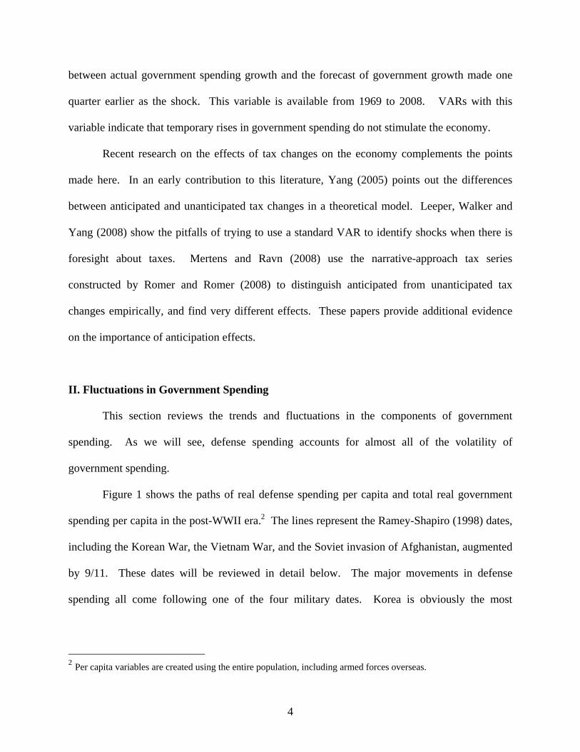
between actual government spending growth and the forecast of government growth made one

quarter earlier as the shock. This variable is available from 1969 to 2008. VARs with this

variable indicate that temporary rises in government spending do not stimulate the economy.

Recent research on the effects of tax changes on the economy complements the points

made here. In an early contribution to this literature, Yang (2005) points out the differences

between anticipated and unanticipated tax changes in a theoretical model. Leeper, Walker and

Yang (2008) show the pitfalls of trying to use a standard VAR to identify shocks when there is

foresight about taxes. Mertens and Ravn (2008) use the narrative-approach tax series

constructed by Romer and Romer (2008) to distinguish anticipated from unanticipated tax

changes empirically, and find very different effects. These papers provide additional evidence

on the importance of anticipation effects.

II. Fluctuations in Government Spending

This section reviews the trends and fluctuations in the components of government

spending. As we will see, defense spending accounts for almost all of the volatility of

government spending.

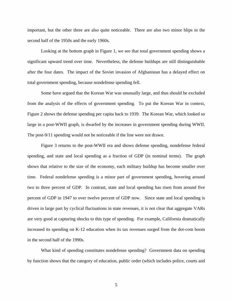
Figure 1 shows the paths of real defense spending per capita and total real government

spending per capita in the post-WWII era.2 The lines represent the Ramey-Shapiro (1998) dates,

including the Korean War, the Vietnam War, and the Soviet invasion of Afghanistan, augmented

by 9/11. These dates will be reviewed in detail below. The major movements in defense

spending all come following one of the four military dates. Korea is obviously the most

2 Per capita variables are created using the entire population, including armed forces overseas.

5

important, but the other three are also quite noticeable. There are also two minor blips in the

second half of the 1950s and the early 1960s.

Looking at the bottom graph in Figure 1, we see that total government spending shows a

significant upward trend over time. Nevertheless, the defense buildups are still distinguishable

after the four dates. The impact of the Soviet invasion of Afghanistan has a delayed effect on

total government spending, because nondefense spending fell.

Some have argued that the Korean War was unusually large, and thus should be excluded

from the analysis of the effects of government spending. To put the Korean War in context,

Figure 2 shows the defense spending per capita back to 1939. The Korean War, which looked so

large in a post-WWII graph, is dwarfed by the increases in government spending during WWII.

The post-9/11 spending would not be noticeable if the line were not drawn.

Figure 3 returns to the post-WWII era and shows defense spending, nondefense federal

spending, and state and local spending as a fraction of GDP (in nominal terms). The graph

shows that relative to the size of the economy, each military buildup has become smaller over

time. Federal nondefense spending is a minor part of government spending, hovering around

two to three percent of GDP. In contrast, state and local spending has risen from around five

percent of GDP in 1947 to over twelve percent of GDP now. Since state and local spending is

driven in large part by cyclical fluctuations in state revenues, it is not clear that aggregate VARs

are very good at capturing shocks to this type of spending. For example, California dramatically

increased its spending on K-12 education when its tax revenues surged from the dot-com boom

in the second half of the 1990s.

What kind of spending constitutes nondefense spending? Government data on spending

by function shows that the category of education, public order (which includes police, courts and

6

prisons), and transportation expenditures has increased to 50 percent of total government

spending The standard VAR approach includes shocks to this type of spending in its analysis

(e.g. Blanchard and Perotti (2002)). Such an inclusion is questionable for several reasons. First,

the biggest part of this category, education, is driven in large part by demographic changes,

which can have many other effects on the economy. Second, these types of expenditures would

be expected to have a positive effect on productivity and hence would have a different effect than

government spending that has no direct production function impacts. As Baxter and King (1993)

make clear, the typically neoclassical predictions about the effects of government spending

change completely when government spending is “productive.” Thus, including these categories

in spending shocks is not the best way to test the neoclassical model versus the Keynesian

model.3

In sum, defense spending is a major part of the variation in government spending around

trend. Moreover, it has the advantage of being the type of government spending least likely to

enter the production function or interact with private consumption. It is for this reason that many

analyses of government spending focus on military spending when studying the macroeconomic

effects of government spending, including early contributions by Barro (1981) and Hall (1986)

as well as more recent contributions by Barro and Redlick (2009) and Hall (2009).

3 Some of the analyses, such as Eichenbaum and Fisher (2005) and Perotti (2007), have tried to address this issue by using only “government consumption” and excluding “government investment.” Unfortunately, this National Income and Product Account distinction does not help. As the footnotes to the NIPA tables state: “Government consumption expenditures are services (such as education and national defense) produced by government that are valued at their cost of production….Gross government investment consists of general government and government enterprise expenditures for fixed assets.” Thus, since teacher salaries are the bulk of education spending, they would be counted as “government consumption.”

7

III. Identifying Government Spending Shocks: VAR vs. Narrative Approaches

A. The VAR Approach

Blanchard and Perotti (2002) have perhaps the most careful and comprehensive approach

to estimating fiscal shocks using VARs. To identify shocks, they first incorporate institutional

information on taxes, transfers, and spending to set parameters, and then estimate the VAR.

Their basic framework is as follows:

ttt UYqLAY += −1),(

where Yt consists of quarterly real per capita taxes, government spending, and GDP. Although

the contemporaneous relationship between taxes and GDP turns out to be complicated, they find

that government spending does not respond to GDP or taxes contemporaneously. Thus, their

identification of government spending shocks is identical to a Choleski decomposition in which

government spending is ordered before the other variables. When they augment the system to

include consumption, they find that consumption rises in response to a positive government

spending shock. Galí et al (2007) use this basic identification method in their study which

focuses only on government spending shocks and not taxes. They estimate a VAR with

additional variables of interest, such as real wages, and order government spending first. Perotti

(2007) uses this identification method to study a system with seven variables. 4

B. The Ramey-Shapiro Narrative Approach

In contrast, Ramey and Shapiro (1998) use a narrative approach to identify shocks to

government spending. Because of their concern that many shocks identified from a VAR are

simply anticipated changes in government spending, they focus only on episodes where Business

4 See the references listed in the introduction to see the various permutations on this basic set-up.

8

Week suddenly began to forecast large rises in defense spending induced by major political

events that were unrelated to the state of the U.S. economy. The three episodes identified by

Ramey and Shapiro were as follows:

Korean War

On June 25, 1950 the North Korean army launched a surprise invasion of South Korea,

and on June 30, 1950 the U.S. Joint Chiefs of Staff unilaterally directed General MacArthur to

commit ground, air, and naval forces. The July 1, 1950 issue of Business Week immediately

predicted more money for defense. By August 1950, Business Week was predicting that defense

spending would more than triple by fiscal year 1952.

The Vietnam War

Despite the military coup that overthrew Diem on November 1, 1963, Business Week

was still talking about defense cuts for the next year (November 2, 1963, p. 38; July 11, 1964, p.

86). Even the Gulf of Tonkin incident on August 2, 1964 brought no forecasts of increases in

defense spending. However, after the February 7, 1965 attack on the U.S. Army barracks,

Johnson ordered air strikes against military targets in North Vietnam. The February 13, 1965,

Business Week said that this action was “a fateful point of no return” in the war in Vietnam.

The Carter-Reagan Buildup

The Soviet invasion of Afghanistan on December 24, 1979 led to a significant turnaround

in U.S. defense policy. The event was particularly worrisome because some believed it was a

possible precursor to actions against Persian Gulf oil countries. The January 21, 1980 Business

9

Week (p.78) printed an article entitled “A New Cold War Economy” in which it forecasted a

significant and prolonged increase in defense spending. Reagan was elected by a landslide in

November 1980 and in February 1981 he proposed to increase defense spending substantially

over the next five years.

These dates were based on data up through 1998. Owing to recent events, I now add the

following date to these war dates:

9/11

On September 11, 2001, terrorists struck the World Trade Center and the Pentagon. On

October 1, 2001, Business Week forecasted that the balance between private and public sectors

would shift, and that spending restraints were going “out the window.” To recall the timing of

key subsequent events, the U.S. invaded Afghanistan soon after 9/11. It invaded Iraq on March

20, 2003.

The military date variable takes a value of unity in 1950:3, 1965:1, 1980:1, and 2001:3,

and zeroes elsewhere. This simple variable has a reasonable amount of predictive power for the

growth of real defense spending. A regression of the growth of real defense spending on current

and eight lags of the military date variable has an R-squared of 0.26.5

To identify government spending shocks, the military date variable is embedded in the

standard VAR, but ordered before the other variables.6 Choleski decomposition shocks to the

5 The R-squared jumps to 0.57 if one scales the variable for the size of the buildup, as in Burnside, Eichenbaum and Fisher (2004). 6 The original Ramey-Shapiro (1998) implementation did not use a VAR. They regressed each variable of interest on lags of itself and the current and lagged values of the military date variable. They then simulated the impact of changes in the value of the military date variable. The results were very similar to those obtained from embedding the military variable in a VAR.

10

military date variable rather than to the government spending variable are used to identify

government shocks.

C. Comparison of Impulse Response Functions

Consider now a comparison of the effects of government spending increases based on the

two identification methods. In both instances, I use a VAR similar to the one used recently by

Perotti (2007) for purposes of comparison. The VAR consists of the log real per capita

quantities of total government spending, GDP, total hours worked, nondurable plus services

consumption, and private fixed investment, as well as the Barro-Redlick (2009) tax rate and the

log of nominal compensation in private business divided by the deflator in private business.7

Chained nondurable and services consumption are aggregated using Whelan’s (2000) method. I

use total hours worked instead of private hours worked based on Cavallo’s (2005) work showing

that a significant portion of rises in government spending consists of increases in the government

payroll. Total hours worked are based on unpublished BLS data and are available on my web

site. Complete details are given in the data appendix. Also, note that I use a product wage rather

than a consumption wage. Ramey and Shapiro (1998) show both theoretically and empirically

why it is the product wage that should be used when trying to distinguish models of government

spending. Defense spending tends to be concentrated in a few industries, such as manufactured

goods. Ramey and Shapiro show that the relative price of manufactured goods rise significantly

7 The results are very similar if I instead use Alexander and Seater’s (2009) update of the Seater (1983) and Stephenson (1998) average marginal tax rate. The Alexander-Seater tax rates are based on actual taxes paid, whereas the Barro-Sahasakul series uses statutory rates. The new Barro-Redlick series includes state income taxes, whereas the Alexander-Seater series only has federal income and social security tax rates.

11

during a defense buildup. Thus, product wages in the expanding industries can fall at the same

time that the consumption wage is unchanged or rising.8

Both VARs are specified in levels, with a quadratic time trend and four lags included.

In the VAR identification, the government spending shock is identified by a Choleski

decomposition in which government spending is ordered first. In the war dates identification, the

current value and four lags of a dummy variable with the military date are also included. The

military date takes a value of unity in 1950:3, 1965:1, 1980:1, and 2001:3.9 I compare the

effects of shocks that are normalized so that the log change of government spending is unity at

its peak in both specifications.

Figures 4A and 4B show the impulse response functions. The standard error bands

shown are only 68% bands. Although this is common practice in the government spending

literature, it has no theoretical justification.10 I only use the narrow error bands because the

wider ones make it is difficult to see the comparison of mean responses across specifications. In

the later analysis with my new variables, I also show 95% error bands.

The first column shows the results from the VAR identification and the second column

shows the results from the war dates identification. Figure 4A shows the effects on government

spending, GDP, and hours. The results are qualitatively consistent across the two identification

schemes for these three variables. By construction, total government spending rises by the same

amount, although the peak occurs several quarters earlier in the VAR identification. This is the

first indication that a key difference between the two methods is timing. GDP rises in both

8 The main reason that Rotemberg and Woodford (1992) find that real wages increase is that they construct their real wage by dividing the wage in manufacturing by the implicit price deflator. Ramey and Shapiro show that the wage in manufacturing divided by the price index for manufacturing falls during a defense buildup. 9 Burnside, Eichenbaum and Fisher (2004) allow the value of the dummy variable to differ across episodes according to the amount that government spending increase. They obtain very similar results. 10 Some have appealed to Sims and Zha (1999) for using 68% bands. However, there is no formal justification for this particular choice. It should be noted that most papers in the monetary literature use 95% error bands.

12

cases, but its rise is much greater in the case of the war dates identification. Hours rise slightly

in the VAR identification, but much more strongly in the war dates identification. A comparison

of the output and hours response shows that productivity rises slightly in both specifications.

Figure 4B shows the cases in which the two identification schemes differ in their

implications. The VAR identification scheme implies that government spending shocks raise

consumption, lower investment for two years, and raise the real wage. In contrast, the war dates

identification scheme implies that government spending shocks lower consumption, raise

investment for a quarter before lowering it, and lower the real wage.

Overall, these two approaches give diametrically opposed answers with regard to some

key variables. The next section presents empirical evidence and a theoretical argument that can

explain the differences.

IV. The Importance of Timing

A concern with the VAR identification scheme is that some of what it classifies as

“shocks” to government spending may well be anticipated. Indeed, my reading of the narrative

record uncovered repeated examples of long delays between the decision to increase military

spending and the actual increase. At the beginning of a big buildup of strategic weapons, the

Pentagon first spends at least several months deciding what sorts of weapons it needs. The task

of choosing prime contractors requires additional time. Once the prime contracts are awarded,

the spending occurs slowly over time. Quarter-to-quarter variations are mostly due to production

scheduling variations among prime contractors.

From the standpoint of the neoclassical model, what matters for the wealth effect are

changes in the present discounted value of government purchases, not the particular timing of the

13

purchases. Thus, it is essential to identify when news becomes available about a major change in

the present discounted value of government spending.

Blanchard and Perotti (2002) worried about the timing issue, and devoted Section VIII of

their paper to analyzing it. To test for the problem of anticipated policy, they included future

values of the estimated shocks to determine whether they affected the results. They found that

the response of output was greater once they allowed for anticipation effects (see Figure VII).

Unfortunately, they did not show how the responses of consumption or real wages were affected.

Perotti (2005) approached the anticipation problem by testing whether OECD forecasts of

government spending predicted his estimated government spending shocks. For the most part,

he found that they did not predict the shocks.

In the next subsection, I show that the war dates as well as professional forecasts predict

the VAR government spending shocks. I also show how in each war episode, the VAR shocks

are positive several quarters after Business Week started forecasting increases in defense

spending. In the second subsection, I present simulations from a simple theoretical model that

shows how the difference in timing can explain most of the differences in results. In the final

subsection, I show that delaying the timing of the Ramey-Shapiro dates produces the Keynesian

results.

A. Empirical Evidence on Timing Lags

To compare the timing of war dates versus VAR-identified shocks, I estimate shocks

using the VAR discussed above except with defense spending rather than total government

spending as the key variable. I then plot those shocks around the war dates.

14

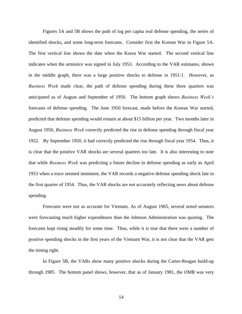
Figures 5A and 5B shows the path of log per capita real defense spending, the series of

identified shocks, and some long-term forecasts. Consider first the Korean War in Figure 5A.

The first vertical line shows the date when the Korea War started. The second vertical line

indicates when the armistice was signed in July 1953. According to the VAR estimates, shown

in the middle graph, there was a large positive shocks to defense in 1951:1. However, as

Business Week made clear, the path of defense spending during these three quarters was

anticipated as of August and September of 1950. The bottom graph shows Business Week’s

forecasts of defense spending. The June 1950 forecast, made before the Korean War started,

predicted that defense spending would remain at about $15 billion per year. Two months later in

August 1950, Business Week correctly predicted the rise in defense spending through fiscal year

1952. By September 1950, it had correctly predicted the rise through fiscal year 1954. Thus, it

is clear that the positive VAR shocks are several quarters too late. It is also interesting to note

that while Business Week was predicting a future decline in defense spending as early as April

1953 when a truce seemed imminent, the VAR records a negative defense spending shock late in

the first quarter of 1954. Thus, the VAR shocks are not accurately reflecting news about defense

spending.

Forecasts were not as accurate for Vietnam. As of August 1965, several noted senators

were forecasting much higher expenditures than the Johnson Administration was quoting. The

forecasts kept rising steadily for some time. Thus, while it is true that there were a number of

positive spending shocks in the first years of the Vietnam War, it is not clear that the VAR gets

the timing right.

In Figure 5B, the VARs show many positive shocks during the Carter-Reagan build-up

through 1985. The bottom panel shows, however, that as of January 1981, the OMB was very

15

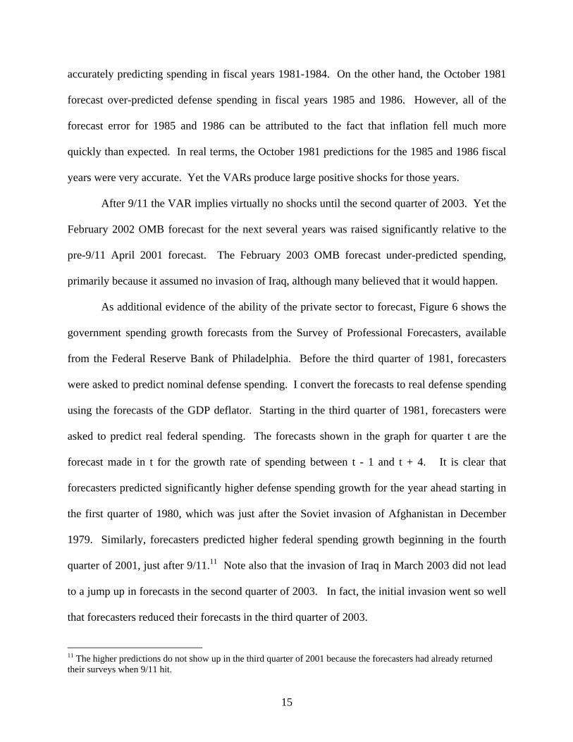
accurately predicting spending in fiscal years 1981-1984. On the other hand, the October 1981

forecast over-predicted defense spending in fiscal years 1985 and 1986. However, all of the

forecast error for 1985 and 1986 can be attributed to the fact that inflation fell much more

quickly than expected. In real terms, the October 1981 predictions for the 1985 and 1986 fiscal

years were very accurate. Yet the VARs produce large positive shocks for those years.

After 9/11 the VAR implies virtually no shocks until the second quarter of 2003. Yet the

February 2002 OMB forecast for the next several years was raised significantly relative to the

pre-9/11 April 2001 forecast. The February 2003 OMB forecast under-predicted spending,

primarily because it assumed no invasion of Iraq, although many believed that it would happen.

As additional evidence of the ability of the private sector to forecast, Figure 6 shows the

government spending growth forecasts from the Survey of Professional Forecasters, available

from the Federal Reserve Bank of Philadelphia. Before the third quarter of 1981, forecasters

were asked to predict nominal defense spending. I convert the forecasts to real defense spending

using the forecasts of the GDP deflator. Starting in the third quarter of 1981, forecasters were

asked to predict real federal spending. The forecasts shown in the graph for quarter t are the

forecast made in t for the growth rate of spending between t - 1 and t + 4. It is clear that

forecasters predicted significantly higher defense spending growth for the year ahead starting in

the first quarter of 1980, which was just after the Soviet invasion of Afghanistan in December

1979. Similarly, forecasters predicted higher federal spending growth beginning in the fourth

quarter of 2001, just after 9/11.11 Note also that the invasion of Iraq in March 2003 did not lead

to a jump up in forecasts in the second quarter of 2003. In fact, the initial invasion went so well

that forecasters reduced their forecasts in the third quarter of 2003.

11 The higher predictions do not show up in the third quarter of 2001 because the forecasters had already returned their surveys when 9/11 hit.

16

Overall, it appears that much of what the VAR might be labeling as “shocks” to defense

spending may have been forecasted. To test this hypothesis formally, I perform Granger

causality tests between various variables and the VAR-based government spending shocks. In

addition to the military dates variable, I also use estimates from the Survey of Professional

Forecasters for real federal government spending forecasts starting in the third quarter of 1981. I

use both the implied forecast dating from quarter t-1 of the log change in real spending from

quarter t-1 to quarter t and the implied forecast dating from quarter t-4 of the change from

quarter t-4 to quarter t..

Table 1 shows the results. The evidence is very clear: the war dates Granger-cause the

VAR shocks but the VAR shocks do not Granger-cause the war dates. Moreover, the VAR

shocks, which are based on information up through the previous quarter, are Granger-caused by

professional forecasts, even those made four quarters earlier. Thus, the VAR shocks are

forecastable.

One should be clear that timing is not an issue only with defense spending. Consider the

interstate highway program. In early 1956, Business Week was predicting that the “fight over

highway building will be drawn out.” By May 5, 1956, Business Week thought that the highway

construction bill was a sure bet. It fact it passed in June 1956. However, the multi-billion dollar

program was intended to stretch out over 13 years. It is difficult to see how a VAR could

accurately reflect this program. Another example is schools for the Baby Boom children.

Obviously, the demand for schools is known several years in advance. Between 1949 and 1969,

real per capita spending on public elementary and secondary education increased 300%.12 Thus,

a significant portion of non-defense spending is known months, if not years, in advance.

12 The nominal figures on expenditures are from the Digest of Education Statistics. I used the GDP deflator to convert to real.

17

B. The Importance of Timing in a Theoretical Model

Macroeconomists have known for a long time that anticipated policy changes can have

very different effects from an unanticipated change. For example, Taylor (1993, Chapter 5)

shows the effects of a change in government spending, anticipated two years in advance, on such

variables as GDP, prices, interest rates and exchange rates. He does not consider the effects on

consumption or real wages, however. More recently, Yang (2005) shows that foresight about tax

rate changes significantly changes the responses of key variables in theoretical simulations.

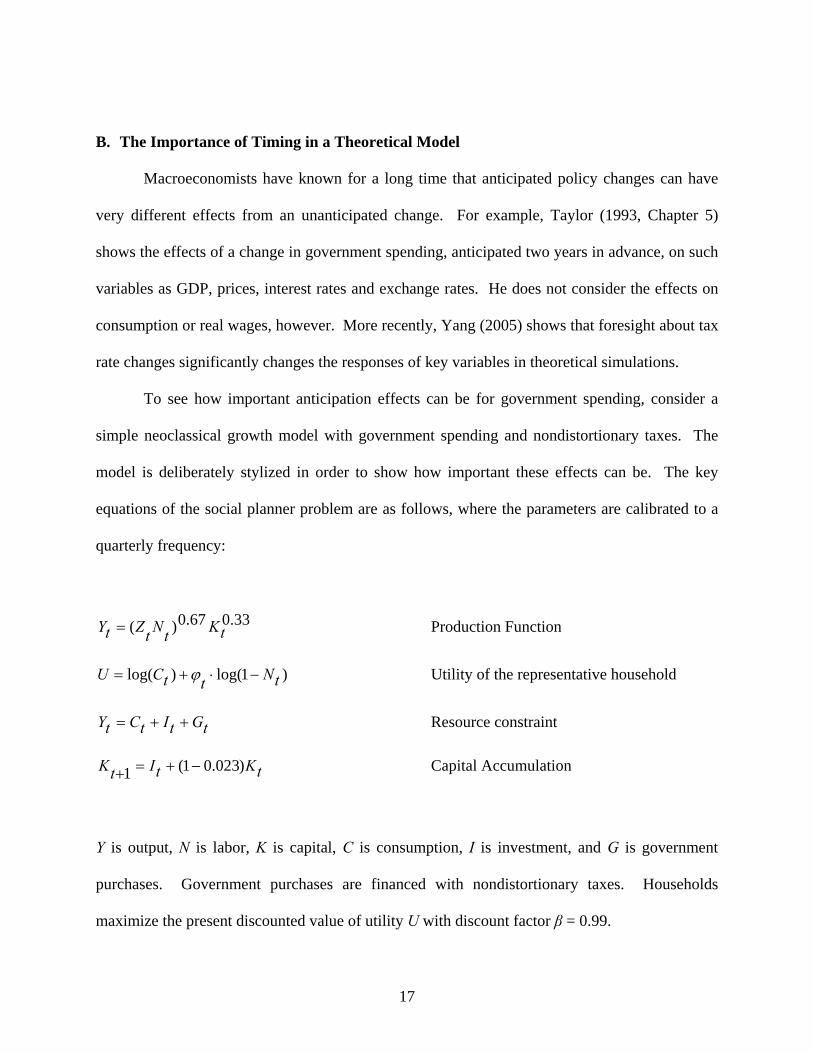
To see how important anticipation effects can be for government spending, consider a

simple neoclassical growth model with government spending and nondistortionary taxes. The

model is deliberately stylized in order to show how important these effects can be. The key

equations of the social planner problem are as follows, where the parameters are calibrated to a

quarterly frequency:

33.067.0)( tKtNtZtY = Production Function

)1log()log( tNttCU −⋅+= ϕ Utility of the representative household

tGtItCtY ++= Resource constraint

tKtItK )023.01(1 −+=+ Capital Accumulation

Y is output, N is labor, K is capital, C is consumption, I is investment, and G is government

purchases. Government purchases are financed with nondistortionary taxes. Households

maximize the present discounted value of utility U with discount factor β = 0.99.

18

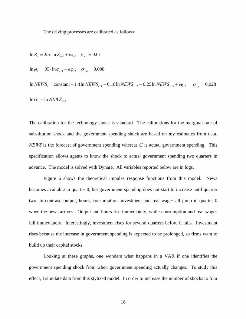
The driving processes are calibrated as follows:

2

321

1

1

lnln

028.0,ln25.0ln18.0ln4.1constant ln

008.0,ln95.ln

01.0,ln95.ln

−

−−−

−

−

=

=+−−+=

=+⋅=

=+⋅=

tt

egttttt

ettt

ezttt

NEWSG

egNEWSNEWSNEWSNEWS

e

ezZZ

σ

σϕϕϕ

σ

ϕ

The calibration for the technology shock is standard. The calibrations for the marginal rate of

substitution shock and the government spending shock are based on my estimates from data.

NEWS is the forecast of government spending whereas G is actual government spending. This

specification allows agents to know the shock to actual government spending two quarters in

advance. The model is solved with Dynare. All variables reported below are in logs.

Figure 6 shows the theoretical impulse response functions from this model. News

becomes available in quarter 0, but government spending does not start to increase until quarter

two. In contrast, output, hours, consumption, investment and real wages all jump in quarter 0

when the news arrives. Output and hours rise immediately, while consumption and real wages

fall immediately. Interestingly, investment rises for several quarters before it falls. Investment

rises because the increase in government spending is expected to be prolonged, so firms want to

build up their capital stocks.

Looking at these graphs, one wonders what happens in a VAR if one identifies the

government spending shock from when government spending actually changes. To study this

effect, I simulate data from this stylized model. In order to increase the number of shocks to four

19

so that I can include at least three variables in the VARs, I also assume that there is measurement

error in the logarithm of output, and that it follows an AR(1) with autocorrelation coefficient of

0.95 and standard errors of 0.005. I then run two types of trivariate VARs on the simulated data.

In the first set of VARs, I use government spending, output, and the variable of interest, and

identify the shock as the shock to government spending, which is ordered first. In the second set

VARs, I use the news, output, and the variable of interest, and identify the shock as the shock to

the news variable which is ordered first. In all cases, I use four lags of the variables.

Figures 7A and 7B show the results.13 The VARs that identify shocks from actual

government spending, are shown in the left column and the VARs that identify shocks from the

news about government spending are shown in the right column. The patterns across the two

columns are strikingly similar to the patterns across the VARs on real data using the two

methods shown in Figures 4A and 4B. In particular, the shocks to government show a much

smaller response of GDP than the shocks to news, just as the standard VAR identification

method finds a smaller response than the Ramey-Shapiro military dates. The same is true of

hours. In Figure 7B, we see that the shocks to actual government spending lead to a rise in

consumption, whereas the shocks to news lead to a fall in consumption. In both cases, real

wages fall, although the pattern is different. The problem with the VAR that identifies shocks

from actual government spending is that it often catches the variables after they have already had

an initial response to the news. The contemporaneous correlation of the estimated shocks using

actual government spending in the VAR with the true shocks is -0.01. The correlation of the

identified shock and the true shock two quarters ago is 0.4, but the timing is off. Thus, the faulty

13 The government spending and output responses shown are from the trivariate VAR that also contains consumption.

20

timing VAR picks up nothing of the true shocks. In contrast, the correlation between the

estimated shocks using the news and the true shocks is 0.97.

As stated above, this model is very stylized in order to make the point in the simplest

possible model. One could modify the theoretical model to incorporate elements such as habit

persistence in consumption and/or adjustment cost in investment. In this case, the true responses

would be more dragged out and missing the timing by two quarters would have a somewhat

smaller effect. However, introducing more realistic lags would likely have changed the impulse

responses just as they did in the previous example.

C. Would Delaying the Ramey-Shapiro Dates Lead to Keynesian Results?

If the theoretical argument of the last section applies to the current situation, then

delaying the timing of the Ramey-Shapiro dates should result in VAR-type Keynesian results.14

To investigate this possibility, I shifted the four military dates to correspond with the first big

positive shock from the VAR analysis. Thus, instead of using the original dates of 1950:3,

1965:1, 1980:1, and 2001:3, I used 1951:1, 1965:3, 1981:4, and 2003:2.

Figure 8 shows the results using the baseline VAR of the previous sections. As predicted

by the theory, the delayed Ramey-Shapiro dates applied to actual data now lead to rises in

consumption and the real wage, similarly to the shocks from the standard VARs. Thus, the heart

of the difference between the two results appears to be the VAR’s delay in identifying the

shocks.

Alternatively, one could try to estimate the VAR and allow future identified shocks to

have an effect. Blanchard and Perotti (2002) did this for output, but never looked at the effects

on consumption or wages. Based on an earlier draft of my paper, Tenhofen and Wolff (2007) 14 This idea was suggested to me by Susanto Basu.

21

analyze such a VAR for consumption and find that when the VAR timing changes, positive

shocks to defense spending lead consumption to fall.

Thus, all of the empirical and theoretical evidence points to timing as being key to the

difference between the standard VAR approach and the Ramey-Shapiro approach. The fact that

the Ramey-Shapiro dates Granger-cause the VAR shocks suggests that the VARs are not

capturing the timing of the news. The theoretical analysis shows that timing is crucial in

determining the response of the economy to news about increases in government spending.

V. A New Measure of Defense News

The previous sections have presented evidence that standard VARs do not properly

measure government spending shocks because changes in government spending are often

anticipated long before government spending actually changes. Although the original Ramey-

Shapiro war dates attempt to get the timing right, the simple dummy variable approach does not

exploit the potential quantitative information that is available.

Therefore, to create a better measure of “news” about future government spending, I read

news sources in order to gather quantitative information about expectations. The defense news

variable seeks to measure the expected discounted value of government spending changes due to

foreign political events. It is this variable that matters for the wealth effect in a neoclassical

framework. The series was constructed by reading periodicals in order to gauge the public’s

expectations. Business Week was the principal source for most of sample because it often gave

detailed predictions. However, it became much less informative after 2001, so I relied more

heavily on newspaper sources. For the most part, government sources could not be used because

they were either not released in a timely manner or were known to underestimate the costs of

22

certain actions. However, when periodical sources were ambiguous, I consulted official sources,

such as the budget. I did not use professional forecasters except for a few examples because the

forecast horizon was not long enough.

The constructed series should be viewed as an approximation to the changes in

expectations at the time. Because there were so many conflicting or incomplete forecasts, I had

to make many judgment calls. In calculating present discounted values, I used the 3-year

Treasury bond rate prevailing at the time. Before the early 1950s, I used the long-term

government bond rate since the other was not available.

If the shock occurred in the last week or two of a quarter, I dated it as the next quarter,

since it could not have much effect on aggregates for the entire current quarter. The detailed

companion paper, “Defense News Shocks, 1939-2008: Estimates Based on News Sources” by

Valerie Ramey (2009), provides more than 100 pages of relevant news quotes and analysis of the

expectations during this 70 year time period.

Table 2 shows the dates and values of the nonzero values of the new military shock

series. Figure 9 shows the shocks as a percent the previous quarter’s nominal GDP. Some of

the shocks, such as the Marshall Plan estimate in 1947:II and the moon mission announcement in

1961:II, were caused by military events but were classified as nondefense spending. While

Roosevelt started boosting defense spending as early as the first quarter of 1939, the first big

shock leading in to World War II was caused by the events leading up to the fall of France, in

1940:II. Thus, my independent narrative analysis supports Gordon and Krenn’s (2009)

contention that fiscal policy became a major force in the economy starting in 1940:II. The

largest single defense news shock (as a percent of GDP) was 1941:IV. As the companion paper

(Ramey (2009)) discusses, estimates of defense spending were skyrocketing even before the

23

Japanese attack on Pearl Harbor on December 7, 1941. Germany had been sinking U.S. ships in

the Atlantic during the fall of 1941, and Business Week proclaimed that American entry into a

“shooting war” was imminent (October 25, 1941, p. 13). It also declared that the U.S. was set

for a Pacific showdown with Japan. The second biggest shock (as a percent of GDP) was the

start of the Korean War. Estimates of defense spending increased dramatically within two

months of North Korea’s attack on South Korea on June 25, 1950.

Table 3 shows how well these shocks predict spending and whether they are relevant

instruments. As Staiger and Stock (1997) discuss, a first-stage F-statistic below 10 could be an

indicator of a weak instrument problem. Unfortunately, most macro “shocks” used in the

literature, such as oil prices and monetary shocks, have F-statistics well below 10.

The numbers shown in Table 3 are for three sample periods: 1939:1 – 2008:4, 1947:1 –

2008:4, and 1955:1 – 2008:4. The first two columns show the R-squared and the F-statistic for

the regression of the growth of real per capita defense spending or total government spending on

current and four lags of “defense news,” which is the present discounted value of the expected

spending change divided by nominal GDP of the previous quarter. The last column shows the F-

statistic on the exclusion of the defense news variable from a regression of the growth of real per

capita defense spending on four lags of log real per capita defense spending, log real GDP, the 3-

month T-bill rate, and the Barro-Redlick average marginal tax rate. These variables will be used

in the VARs to follow, so it is important to determine the marginal F-statistic of the new shock

variable.

The table shows that as long as WWII or the Korean War is included, the new military

shock variable has significant explanatory power and is a strongly relevant instrument. The R-

squared for the sample from 1939 to 2008 is 0.42 and from 1947 to 2008 is 0.55. All of the F-

24

statistics in the first two samples are just below or well above 10. On the other hand, for the

sample that excludes WWII and the Korean War, the shock variable has much less explanatory

power and the F-statistics are well below the comfortable range. All indications are that this

variable is not informative for the period after the Korean War.

I next consider the effect of the defense news variable in a VAR. Since timing is

important, I use quarterly data rather than annual data. Therefore, I must construct quarterly data

for the 1939 to 1946 period since the BEA currently reports only annual data from that period.

Fortunately, a 1954 BEA publication reports estimates of quarterly nominal components of GDP

back to 1939. I combined these data with available price indices from the BLS to create real

series. I used these constructed series to interpolate current annual NIPA estimates. The data

appendix contains more details.

One is always worried when interpolation of data is involved, since the method and data

used might make a difference. Fortunately, Gordon and Krenn (2009) have independently

created a valuable new dataset for their research analyzing the role of government spending in

ending the Great Depression. In their paper, they use completely different data sources and

interpolation methods to construct macroeconomic data from 1919 to 1954. In private

correspondence, we compared our series for the overlap period starting in 1939 and found them

to be remarkably similar.

In order to examine the effect on a number of variables without including too many

variables in the VAR, I follow Burnside, Eichenbaum, and Fisher’s (2004) strategy of using a

fixed set of variables and rotating other variables of interest in. The fixed set of variables

consists of defense news, the log of real per capita government spending, the log of real per

capita GDP, the three-month T-bill rate, and the Barro-Redlick average marginal income tax rate.

25

These last two variables are included in order to control for monetary policy and tax policy.15 To

the fixed set of five variables, I rotate in a series of sixth variables, one at a time. The extra

variables considered are total hours, the manufacturing product wage (the only consistent wage

series back to 1939), the real BAA bond rate (with inflation defined by the CPI), the three

components of consumer expenditures, nonresidential investment and residential investment.

Four lags of the variables are used and a quadratic time trend is included. The data appendix

fully describes all of the data used in the VAR, including the extensive construction of quarterly

data for the WWII era.

Figures 10A and 10B shows the impulse response functions to a shock in the defense

news variable. As before, the responses are normalized so that the government spending

response to defense news is equal to unity. In the impulse responses shown earlier, I only

included 68% standard error bands so that the graphs could be more easily compared across

specifications. Here, I also show the more conventional 95% standard error bands.

After a positive defense news shock, total government spending rises, peaking six

quarters after the shock and returning to normal after four years. GDP also increases

significantly, peaking six quarters after the shock and returning to normal after four years. The

implied elasticity of the GDP peak with respect to the government spending peak is 0.2. Since

the average ratio of nominal GDP to nominal government spending was 4.9 from 1939 to 2008,

the implied government spending multiplier implied by these estimates is 1.0. If, instead, I

calculate the multiplier by using the integral under the impulse response function for the five

years after the shock, estimate of the multiplier is only slightly higher, at 1.1.

15 Rossi and Zabairy (2009) make the case that analyses of fiscal policy should always control for monetary policy and vice versa.

26

Figure 10A also shows that total hours increases, significantly even by conventional

significance levels. A comparison of the peak of the hours response to the peak of the GDP

response implies that productivity also increases. McGrattan and Ohanian (forthcoming) argue

that the neoclassical model can only explain the behavior of macroeconomic variables during

WWII if there were also positive TFP shocks. Positive TFP shocks are one possible explanation,

although learning-by-doing (extensively documented during WWII) or increasing returns to scale

are other possibilities. The real product wage in manufacturing initially falls and then rises.

Thus, the manufacturing product wage appears to be following the path of labor productivity.

The 3-month Treasury bill rate falls slightly after a positive defense news shock, but it is

not significantly different from zero. This response is most likely due to the response of

monetary policy, particularly during WWII and the Korean War. On average, the income tax

rate increases significantly after a positive spending shock.

Figure 10B shows six more variables of interest. The first panel shows that the real

interest rate on BAA bonds initially falls significantly for a year, then rises above zero, before

falling somewhat again. Some of this pattern is likely due to the erratic behavior of inflation. In

both World War II and the Korean War, prices shot up on the war news in anticipation of price

controls. The next panel shows that nondurable consumption expenditures fall significantly at

conventional significance levels. In contrast, consumption expenditures on services rises

significantly. Oddly, this variable stays well above normal even after GDP has returned to

normal. Consumer durable purchases fall significantly. In addition, the stock of consumer

durable goods as well as total consumption expenditures (not shown) also fall significantly.

Finally, both nonresidential investment and residential investment fall significantly.

27

To summarize, except for services consumption, all other components of consumption

and investment fall, consistent with the negative wealth effect of neoclassical theory. On the

other hand, the rise in productivity and the real product wage are inconsistent with the

neoclassical model. The multiplier is estimated to be between 1.0 and 1.1.

Figures 11A and 11B compare the impulse responses from the VARs estimated from

1939 to 2008 to the ones estimated from 1947 to 2008. Again, the peak of government spending

is normalized to be one. The upper right panel of Figure 11A shows the response of GDP is

somewhat less when WWII is excluded. The peak response is 0.21 with WWII included but 0.16

when WWII is excluded. This response implies a government spending multiplier of 0.78. If

instead I calculate the multiplier using the integral of the impulse response functions, the

multiplier is estimated to be 0.6. As Ohanian (1997) argues, spending during WWII was

financed mostly by issuing debt, whereas spending during the Korean War was financed in large

part by increases in taxes. Thus, the differential multiplier might be attributable to the effect of

less use of distortionary business taxes during WWII.

The hours response is somewhat smaller when WWII is omitted. In contrast to the earlier

results, the manufacturing product wage decreases significantly if WWII is excluded. The

increase in the manufacturing product wage during World War II could be due to differential

strengths of wage and price controls. Finally, the 3-month Treasury bill rate falls much more

when WWII is omitted.

Figure 11B compares the responses with and without WWII for real interest rates,

consumption and investment. The responses of both real interest rates and nondurable

consumption are similar with and without WWII. In contrast, services consumption moves little

if WWII is excluded. Consumer durable purchases fall in both samples, but there is an initial

28

rise when WWII is excluded. This rise is dominated by the beginning of the Korean War, when

consumers with recent memories of WWII feared that rationing was imminent. Finally,

residential investment falls much less and turns positive after two years when WWII is excluded.

The results for the sample from 1955 to 2008 (not shown) are unusual. In particular,

GDP rises for one period and then becomes negative after a positive defense shock. The

standard error bands are very wide, though. As discussed above, the preliminary diagnostics

indicate that the defense news variable is not very informative for government spending in a

sample that excludes the two big wars. On the other hand, the impulse responses estimated on a

sample that includes WWII, but excludes Korea, look very similar to those from the entire

sample.

The multipliers estimated here, around 1.0 for the sample with WWII and 0.6 to 0.8 for

the post-WWII sample, lie in the range of most other estimates from the literature. In his recent

paper, Hall (2009) regresses the growth of real GDP on the growth of real defense spending

using annual data. In the sample from 1930 to 2008, he finds a multiplier of 0.55; for 1947 to

2008, he finds a multiplier of 0.47. Barro and Redlick (2009) use annual data from 1914 to 2006

and find multipliers between 0.6 and 1. In contrast, Fisher and Peters (2009), using excess

returns on defense stocks find a total government spending multiplier of 1.5. I will discuss

details of their paper in the next section.

To summarize, the results based on VARs using the richer news variable back to 1939

largely support the qualitative results from the simpler Ramey-Shapiro military date variable.

Most measures of consumption fall. Although the product wage in manufacturing rises if WWII

is included, it falls when WWII is excluded.

29

VI. Post-Korean War News Shocks Based on Professional Forecasts

As discussed in the last section, the defense news variable is not very informative for the

post-Korean War sample. Both the R-squared and the first-stage F-statistic are very low. Thus,

the VAR finding that output and hours fall after a positive government spending shock in this

later period are suspect. In order to study this later time period, I construct a second news

variable based on professional forecasters. This variable measures the one-quarter ahead

forecast error, based on the survey of professional forecasters. As discussed above, I have

already shown that the professional forecasts Granger-cause the standard VAR shocks. Thus,

this measure of news is likely to have fewer anticipation effects than the standard VAR shock.

From the fourth quarter of 1968 to the second quarter of 1981, the Survey of Professional

Forecasters predicted nominal defense spending. I convert the forecast of nominal spending to a

forecast of real spending using the forecasters’ predictions about the GDP deflator. For this

period, I define the shock as the difference between actual real defense spending growth between

t-1 and t and the forecasted growth of defense spending for the same period, where the forecast

was made in quarter t-1. From the third quarter of 1981 to the present, the forecasters predicted

real federal spending. I construct the shock based on the actual and predicted growth of real

federal spending from period t-1 to t. As Table 4 shows, this shock has an R-squared of 60

percent for government spending growth and F-statistics exceeding 200. Thus, they are

potentially more powerful indicators of news.

I then study the effects of this shock in the same VAR used for the defense news shock,

with the forecast shock substituted for the defense news shock. All other elements of the

specification are the same. Figures 12A and 12B show the effects of this shock on the key

30

variables. Unlike the case with defense spending news shocks in which government spending

has a hump-shaped response, this shock leads government spending to spike up temporarily and

then fall to normal and then negative after a couple of quarters. GDP rises slightly on impact,

but then turns negative. The multiplier computed using the peak responses is around 0.8; the

multiplier computed using the integral under the impulse response functions is negative. Thus,

these shocks lead to rather contractionary effects, similar to those I found for the 1955 to 2008

period with my defense news shocks.16

A recent paper by Fisher and Peters (2009) has taken another promising approach to

constructing news series for government spending by using excess returns on defense stocks.

Their series is not informative for the big wars, such as WWII and the Korean War because

excess profits tax limited the stock returns of defense contractors.17 For the post-Korean War

period, however, it usually matches up well with the Ramey-Shapiro dates. A key exception is

the second half of the 1970s, when the cumulative excess returns increase much earlier than the

narrative method suggests they should. This discrepancy might be explained by the fact that

after the 1973 war in the Middle East, defense contractor sales to foreign governments started to

increase dramatically until they were one-third the size of the U.S. defense procurement budget

(Business Week 12/20/1976, p. 79). Thus, the increase in returns could be due to foreign arms

sales rather than anticipations of increases in the U.S. defense budget. Further evidence in favor

of this hypothesis is provided by Figure 1 of Fisher and Peters’ (2009) paper, which shows that

contractor sales started increasing several years before U.S. military spending increased.

16 These results also hold in a variety of specifications. For example, when I limit the sample to 1981:3 – 2008:4 so that the news shock variable refers only to federal spending, I find similar results. 17 Several years ago, I had initially tried to construct a series based on defense stock returns, but had abandoned it when I realized that defense stocks did not perform better during WWII and the Korean War. Fisher and Peters wisely limited their sample to the post-Korean War period.

31

Fisher and Peters (2009) show that after a shock to the cumulative excess returns to

defense contractor stocks during the post-Korean War period, government spending begins rising

almost immediately, reaches a new plateau after 10 quarters, and shows little indication of falling

for at least 20 quarters. On the other hand, output, hours, and consumption either stay constant

or decline for five quarters, and then rise with a hump-shape. The consumption response is not

significantly different from zero at conventional levels, though.18 On the other hand, real wages

fall significantly and then become indistinguishable from zero. Their multiplier is estimated to

be 1.5.

Thus, the shocks identified from Fisher and Peters’ (2009) defense stocks excess returns

imply much more persistent rises in government spending and much higher multipliers than

implied by most other shocks studied, including those from a standard VAR, the defense news

variable based on the narrative method, as well as professional forecast errors. In contrast, my

new shock based on professional forecast errors implies more temporary changes in government

spending and smaller multipliers than the other methods. Therefore, in order to understand why

the responses of macroeconomic variables are different, it would be useful to analyze why the

responses of government spending to the various shocks have such different persistence.

VI. Conclusions

This paper has explored possible explanations for the dramatically different results

between standard VAR methods and the narrative approach for identifying shocks to government

spending. I have shown that the main difference is that the narrative approach shocks appear to

capture the timing of the news about future increases in government spending much better. In

18 Fisher and Peters (2009) show 68 percent confidence bands. As discussed earlier, there is no econometric basis for using this low level of significance for hypothesis testing.

32

fact, these shocks Granger-cause the VAR shocks. My theoretical results show how timing can

account for all of the difference in the results across the two methods. Because the VAR

approach captures the shocks too late, it misses the initial decline in consumption and real wages

that occurs as soon as the news is learned. I show that delaying the timing on the Ramey-

Shapiro dates replicates the VAR results.

Finally, I have constructed two new series of government spending shocks. The first

series improves on the basic Ramey-Shapiro war dates by extending the analysis back to WWII

and by computing the expected present discounted value of changes in government spending.

This variable produces results that are qualitatively similar to those obtained from the simple war

dates variable: in response to an increase in government spending, most measures of

consumption and real wages fall. However, the implied multipliers are lower: the implied

multiplier is unity when WWII is included and 0.6 to 0.8 when World War II is excluded. It

should be understood that this multiplier is estimated on data in which distortionary taxes

increase on average during a military build-up, and is not necessarily applicable to situations in

which government spending is financed differently.

Since the defense news variable is much less informative for the most recent period, I

also construct a second news series, based on forecast errors of professional forecasters. Shocks

to this series imply that temporary rises in government spending generally lead to declines in

output, hours, consumption and investment. Thus, none of my results indicate that government

spending has multiplier effects beyond its direct effect.

33

Data Appendix

Construction of the New Military Series See Ramey (2009) “Defense News Shocks, 1939-2008: Estimates Based on News Sources” for complete documentation. Data for 1947 – 2008 Data on nominal GDP, quantity indexes of GDP, and price deflators for GDP and its components were extracted from bea.gov on August 30, 2009. The combined category of real consumption nondurables plus services was created using Wheelan’s (2000) method. The quarterly stock of consumer durables was created by interpolating annual data on the quantity index for the net stock of consumer durables with the quantity index of consumer durable purchases. The Denton module for Stata (Baum (2008)) was used to interpolate the annual change in the stock with purchases, and then was integrated.

The nominal wage and price index for business were extracted August 2009 from bls.gov productivity program.

The total hours data used in the baseline post-WWII regressions is from unpublished data from the BLS, kindly provided by Shawn Sprague. Data for 1939 - 1946 NIPA Data: National Income, 1954 Edition, A Supplement to the Survey of Current Business presents quarterly nominal data on GNP and its components going back to 1939. Although the levels are somewhat different, the quarterly correlation of these data with modern data for the overlap between 1947 and 1953 is 0.999. To create quarterly real GDP, I first constructed price deflators for various components. The price deflators that were available either monthly or quarterly were the Producer Price Index (available from FRED), the Consumer Price Index (total, nondurables, durables, and services), available from bls.gov, and the price index for manufacturing. For this latter series, I spliced together data from old Survey of Current Business’ with data from bls.gov, which was available from 1986. Based on quarterly regressions of log changes in the various deflators on log changes in these price indexes for 1947 through 1970, I used the following relationships. For each component of consumption, as well as total consumption, I used the relevant CPI index. For nonresidential investment deflator inflation, I used weights on 0.5 each on the CPI inflation and manufacturing inflation. For the residential investment deflator inflation, I used a weight of 0.7 on CPI inflation and 0.3 on manufacturing inflation. The total fixed investment deflator inflation was a weighted average of residential and nonresidential, with the weights varying over time depending on the ratio of nominal nonresidential investment to total fixed investment. For defense (as well as federal and total government spending), I used a weight of 0.3 on CPI inflation and 0.7 on manufacturing inflation. For GDP, I used a weighted average of CPI inflation and manufacturing inflation based on the ratios of the nominal values of defense and investment to GDP, and the component series weights on each type of inflation. Deflators were obtained taking exponentials of the integrated log changes. I used these constructed real

34

quantities to interpolate the quantity indexes for GDP and its components, extracted August 2009 from the BEA website, with the Baum (2008) Stata module of the proportional Denton method. Hours: Kendrick (1961) reports annual civilian and total hours series extending back to the late 1800s. An advantage of Kendrick’s civilian series is that it includes hours worked by “emergency workers” as part of the WPA, etc. Thus, I interpolate Kendrick’s annual series to a quarterly series. I constructed several components for the quarterly interpolation. Various issues of the Statistical Abstract (available online through census.gov) report quarterly or monthly data on employed persons and average weekly hours of employment persons for civilians starting from the 1941:III through 1945. In 1946, ranges of hours were reported, so that average weekly hours could be constructed. Thus, a total hours series for civilians was constructed from these numbers from 1941:III – 1946:IV. However, this series did not include the hours of emergency workers. The number of employed civilians was reported from 1940:2 on, but average hours were not reported. For 1939:I to 1941:II, the only available series was civilian nonfarm employment. I used each of these pieces to interpolate the Kendrick civilian series to a quarterly frequency. (To preserve the seasonal factors from agriculture, I used the information on seasonality in farm hours after 1941 to reproduce the seasonality.) Because this series was based on household data, I spliced it to the CPS household series from 1947 on and seasonally adjusted the entire series using the Census’ X12 program, allowing for outliers due to roving Easters and Labor Days. The seasonally unadjusted CPS monthly data were collected by Cociuba, Prescott, and Ueberfeldt (2009). The military hours series was available quarterly from unpublished BLS data from 1948 on. For 1939 to 1947, I inferred military hours from the annual number of active duty military, assuming that hours per military employee were the same as in 1948. I then interpolated the annual series. Note the hours estimated by the BLS, and hence my series, are about six percent higher than Kendrick’s estimates of military hours. Siu (2008) argues that Kendrick underestimates military hours. Tax Series Barro and Redlick (2009) provide an update for the Barro-Sahasakul (1983) average marginal tax rate series through 2006. I had previously updated Alexander and Seater’s (2009) series through 2007 using their programs. I assumed that the Barro-Redlick series changed by the same percent in 2007 as my update of the Alexander-Seater (2009) series and (for want of more information) was constant through 2008. Survey of Professional Forecasters Series The forecasts of federal spending from 1981:3 on are available online from the Philadelphia Federal Reserve. GDP deflator forecasts were also available online. Thomas Stark kindly provided the forecasts of defense spending from 1968:4 to 1981:2.

35

References

Aiyagari, Rao, Laurence Christiano and Martin Eichenbaum, “The Output, Employment and Interest Rate Effects of Government Consumption.” Journal of Monetary Economics 30 (1992), pp. 73–86.

Alexander, Erin and John Seater, “The Federal Income Tax Function,” North Carolina State

University Working Paper, January 2009. Barro, Robert J., “Output Effects of Government Purchases,” The Journal of Political Economy

89 (December 1981): 1086-1121. Barro, Robert J. and Chaipat Sahasakul, “Measuring the Average-Marginal Tax Rate from the

Individual Income Tax,” Journal of Business, 56 (1983), pp. 419-452. Barro, Robert J. and Charles J. Redlick, “Macroeconomic Effects from Government Purchases

and Taxes,” NBER working paper 15369, September 2009. Baum, Christopher F., “DENTON: Stata Module to Interpolate a Quarterly Flow Series from

Annual Totals via Proportional Denton Method,” Boston College, Revised 2008. Baxter, Marianne and Robert G. King, “Fiscal Policy in General Equilibrium,” American

Economic Review 83 (1993), pp. 315–334. Blanchard, Olivier and Roberto Perotti, “An Empirical Characterization of the Dynamic Effects

of Changes in Government Spending and Taxes on Output,” Quarterly Journal of Economics (November 2002): 1329-1368.

Burnside, Craig, Martin Eichenbaum, and Jonas Fisher, “Fiscal Shocks and their Consequences,”

Journal of Economic Theory 115 (2004): 89-117. Caldara, Dario and Christophe Kamps, “What are the Effects of Fiscal Policy Shocks? A VAR-

based Comparative Analysis,” September 2006 working paper. Cavallo, Michele, “Government Employment Expenditure and the Effects of Fiscal Policy

Shocks,” Federal Reserve Bank of San Francisco Working Paper 2005-16, 2005. Cociuba, Simona, Edward C. Prescott, Alexander Ueberfeldt, “U.S. Hours and Productivity

Behavior Using CPS Hours Worked Data: 1947:III-2009:II,” Working Paper, Federal Reserve Bank of Dallas.

Cullen, Joseph and Price V. Fishback, “Did Big Government Largesse Help the Locals? The

Implications of WWII Spending for Local Economic Activity, 1939-1958.” NBER Working Paper 12801, December 2006.

36

Devereux, Michael, A. C. Head and M. Lapham, “Monopolistic Competition, Increasing Returns, and the Effects of Government Spending,” Journal of Money, Credit, and Banking 28 (1996), pp. 233–254.

Edelberg, Wendy, Martin Eichenbaum and Jonas D. M. Fisher, “Understanding the Effects of a

Shock to Government Purchases,” Review of Economic Dynamics 2 (January 1999): 166-206.

Eichenbaum, Martin and Jonas D. M. Fisher, “Fiscal Policy in the Aftermath of 9/11,” Journal of

Money, Credit, and Banking 37 (February 2005): 1-22. Fatas, Antonio and Ilian Mihov, “The Effects of Fiscal Policy on Consumption and Employment:

Theory and Evidence,” CEPR Discussion Paper No. 2760, April 2001. Fisher, Jonas D.M. and Ryan Peters, “Using Stock Returns to Identify Government Spending

Shocks,” Federal Reserve Bank of Chicago manuscript, August 2009. Gali, Jordi, J. David López-Salido, and Javier Vallés, “Understanding the Effects of Government

Spending on Consumption,” Journal of the European Economic Association, 5 (March 2007): 227-270.

Giavazzi, Francesco and Marco Pagano, “Can Severe Fiscal Contractions be Expansionary?”

NBER Macroeconomics Annual, 1990. Gordon, Robert J. and Robert Krenn, “The End of the Great Depression: VAR Insight on the

Roles of Monetary and Fiscal Policy,” September 2009 working paper. Hall, Robert E., “The Role of Consumption in Economic Fluctuations,” in Robert J. Gordon, ed.

The American Business Cycle: Continuity and Change Chicago: NBER and The University of Chicago Press, 1986.

-----------, “By How Much Does GDP Rise If the Government Buys More Output?” August 2009

manuscript. Kendrick, John W., Productivity Trends in the United States, Princeton: NBER and Princeton

University Press, 1961. Leeper, Eric M., Todd B. Walker, Shu-Chun Susan Yang, “Fiscal Foresight: Analytics and

Econometrics,” NBER Working paper 14028, May 2008. McGrattan, Ellen R. and Lee E. Ohanian, “Does Neoclassical Theory Account for the Effects of

Big Fiscal Shocks? Evidence from World War II,” forthcoming International Economic Review.

McMahon, Robert, The Cold War: A Very Short Introduction, Oxford: Oxford University Press,

2003.

37

Mertens, Karel and Morten O. Ravn, “The Aggregate Effects of Anticipated and Unanticipated

U.S. Tax Policy Shocks: Theory and Empirical Evidence,” May 2008. Mountford, Andrew and Harald Uhlig, “What are the Effects of Fiscal Policy Shocks?” CEPR

Discussion Paper 3338, 2002. Ohanian, Lee E., “The Macroeconomic Effects of War Finance in the United States: World War

II and the Korean War,” American Economic Review 87(March 1997): 23-40. Pappa, Evi, “New Keynesian or RBC Transmission? The Effects of Fiscal Shocks in Labor

Markets,” LSE discussion paper. Perotti, Roberto, “Estimating the Effects of Fiscal Policy in OECD Countries,” CEPR Discussion

Paper 4842, January 2005. -------------------, “In Search of the Transmission Mechanism of Fiscal Policy,” forthcoming

NBER Macroeconomics Annual 2007. Ramey, Valerie A. and Matthew Shapiro, “Costly Capital Reallocation and the Effects of

Government Spending,” Carnegie Rochester Conference on Public Policy (1998). Ramey, Valerie A., “Defense News Shocks, 1939-2008: An Analysis Based on News Sources,”

October 2009 manuscript. http://econ.ucsd.edu/~vramey/research/Defense_News_Narrative.pdf .

Romer, Christina D. and David H. Romer, “The Macroeconomic Effects of Tax Changes:

Estimates Based on a New Measure of Fiscal Shocks,” NBER Working Paper 13264, July 2007.

Rossi, Barabara and Sarah Zubairy, “What is the Importance of Monetary and Fiscal Shocks in

Explaining US Macroeconomic Fluctuations,” Duke manuscript, 2009. Rotemberg, Julio and Woodford, Michael, “Oligopolistic Pricing and the Effects of Aggregate

Demand on Economic Activity,” Journal of Political Economy 100 (1992), pp. 1153–1297.

Seater, John, “Marginal Federal Personal and Corporate Income Tax Tates in the US, 1909-

1975,”. Journal of Monetary Economics, 10, (1982), pp. 361-381. Sims, Christopher A. and Tao Zha, “Error Bands for Impulse Response Functions,”

Econometrica 67 (September 1999): 1113-1155. Siu, Henry, “The Fiscal Role of Conscription in the U.S. World War II Effort,” Journal of

Monetary Economics 55 (September 2008): 1094-1112.

38

Staiger, Doublas and James H. Stock, “Instrumental Variables Regression with Weak Instruments,” Econometrica 65 (May 1997): 557-586.

Stephenson, E. Frank, “Average Marginal Tax Rates Revisited,” Journal of Monetary Economics

41 (April 1998): 389-409. Taylor, John B., Macroeconomic Policy in a World Economy, New York: W.W. Norton, 1993.

(Available online at: http://www.stanford.edu/~johntayl/MacroPolicyWorld.htm ) Tenhofen, Jorn and Guntram Wolff, “Does Anticipation of Government Spending Matter?

Evidence from an Expectations Augmented VAR,” Deutsche Bundesbank working paper, 2007.

Whelan, Karl, “A Guide to the Use of Chain Aggregated NIPA Data,” June 2000 working paper. Yang, Shu-Chun Susan, “Quantifying Tax Effects under Policy Foresight,” Journal of Monetary

Economics 52 (November 2005): 1557-1568.

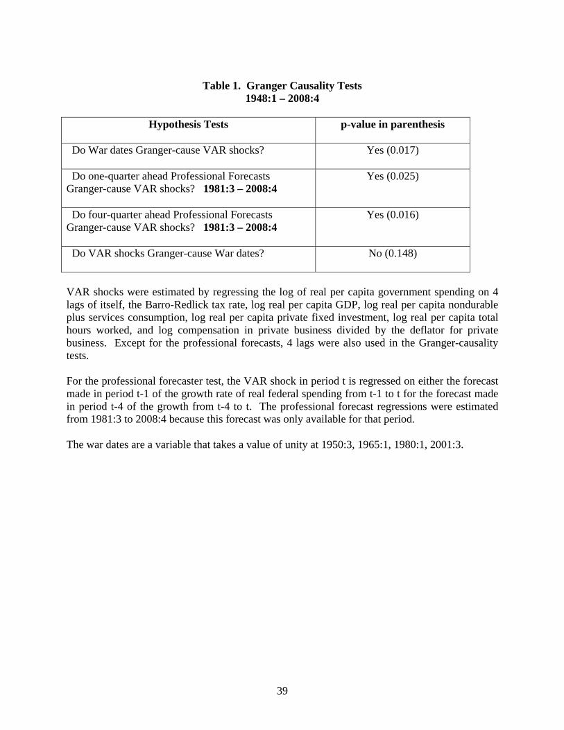
39

Table 1. Granger Causality Tests

1948:1 – 2008:4

Hypothesis Tests

p-value in parenthesis

Do War dates Granger-cause VAR shocks?

Yes (0.017)

Do one-quarter ahead Professional Forecasts Granger-cause VAR shocks? 1981:3 – 2008:4

Yes (0.025)

Do four-quarter ahead Professional Forecasts Granger-cause VAR shocks? 1981:3 – 2008:4

Yes (0.016)

Do VAR shocks Granger-cause War dates?

No (0.148)

VAR shocks were estimated by regressing the log of real per capita government spending on 4 lags of itself, the Barro-Redlick tax rate, log real per capita GDP, log real per capita nondurable plus services consumption, log real per capita private fixed investment, log real per capita total hours worked, and log compensation in private business divided by the deflator for private business. Except for the professional forecasts, 4 lags were also used in the Granger-causality tests. For the professional forecaster test, the VAR shock in period t is regressed on either the forecast made in period t-1 of the growth rate of real federal spending from t-1 to t for the forecast made in period t-4 of the growth from t-4 to t. The professional forecast regressions were estimated from 1981:3 to 2008:4 because this forecast was only available for that period. The war dates are a variable that takes a value of unity at 1950:3, 1965:1, 1980:1, 2001:3.

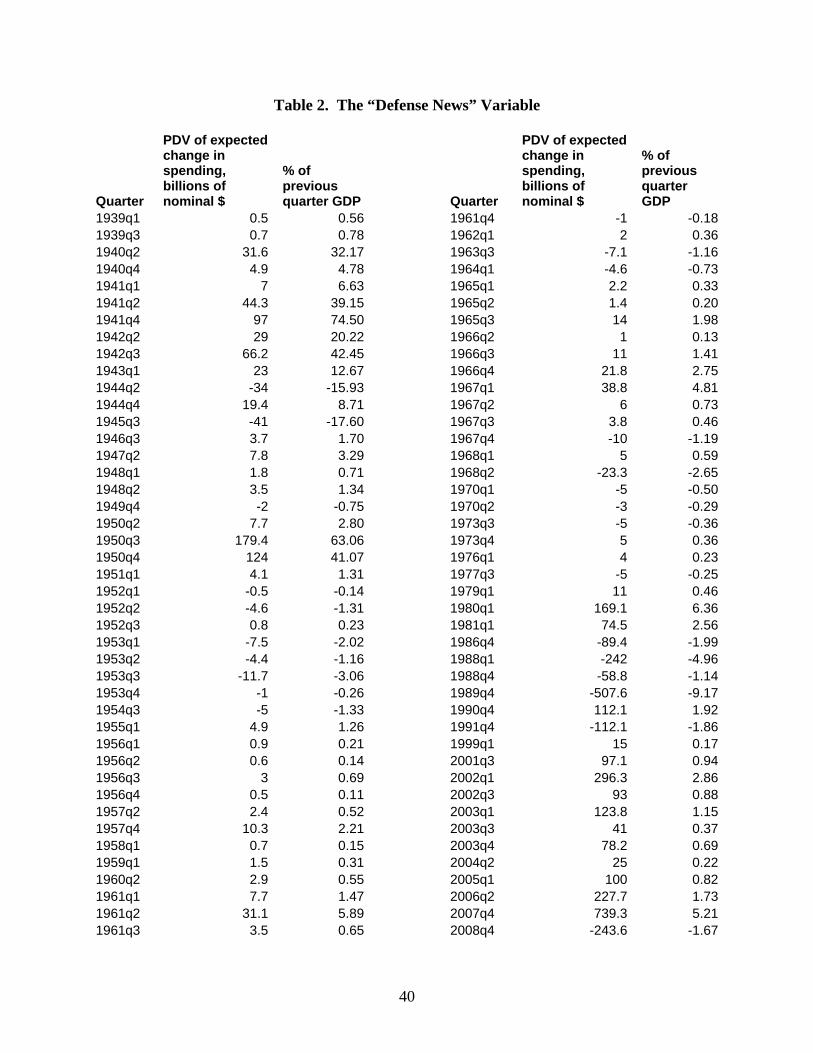
40

Table 2. The “Defense News” Variable

Quarter

PDV of expected change in spending, billions of nominal $

% of previous quarter GDP Quarter

PDV of expected change in spending, billions of nominal $

% of previous quarter GDP

1939q1 0.5 0.56 1961q4 -1 -0.181939q3 0.7 0.78 1962q1 2 0.361940q2 31.6 32.17 1963q3 -7.1 -1.161940q4 4.9 4.78 1964q1 -4.6 -0.731941q1 7 6.63 1965q1 2.2 0.331941q2 44.3 39.15 1965q2 1.4 0.201941q4 97 74.50 1965q3 14 1.981942q2 29 20.22 1966q2 1 0.131942q3 66.2 42.45 1966q3 11 1.411943q1 23 12.67 1966q4 21.8 2.751944q2 -34 -15.93 1967q1 38.8 4.811944q4 19.4 8.71 1967q2 6 0.731945q3 -41 -17.60 1967q3 3.8 0.461946q3 3.7 1.70 1967q4 -10 -1.191947q2 7.8 3.29 1968q1 5 0.591948q1 1.8 0.71 1968q2 -23.3 -2.651948q2 3.5 1.34 1970q1 -5 -0.501949q4 -2 -0.75 1970q2 -3 -0.291950q2 7.7 2.80 1973q3 -5 -0.361950q3 179.4 63.06 1973q4 5 0.361950q4 124 41.07 1976q1 4 0.231951q1 4.1 1.31 1977q3 -5 -0.251952q1 -0.5 -0.14 1979q1 11 0.461952q2 -4.6 -1.31 1980q1 169.1 6.361952q3 0.8 0.23 1981q1 74.5 2.561953q1 -7.5 -2.02 1986q4 -89.4 -1.991953q2 -4.4 -1.16 1988q1 -242 -4.961953q3 -11.7 -3.06 1988q4 -58.8 -1.141953q4 -1 -0.26 1989q4 -507.6 -9.171954q3 -5 -1.33 1990q4 112.1 1.921955q1 4.9 1.26 1991q4 -112.1 -1.861956q1 0.9 0.21 1999q1 15 0.171956q2 0.6 0.14 2001q3 97.1 0.941956q3 3 0.69 2002q1 296.3 2.861956q4 0.5 0.11 2002q3 93 0.881957q2 2.4 0.52 2003q1 123.8 1.151957q4 10.3 2.21 2003q3 41 0.371958q1 0.7 0.15 2003q4 78.2 0.691959q1 1.5 0.31 2004q2 25 0.221960q2 2.9 0.55 2005q1 100 0.821961q1 7.7 1.47 2006q2 227.7 1.731961q2 31.1 5.89 2007q4 739.3 5.211961q3 3.5 0.65 2008q4 -243.6 -1.67

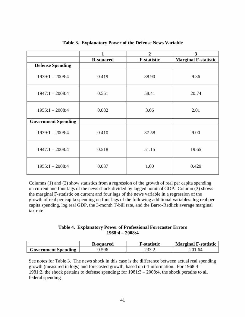
41

Table 3. Explanatory Power of the Defense News Variable

1 2 3 R-squared F-statistic Marginal F-statistic

Defense Spending

1939:1 – 2008:4

0.419

38.90

9.36

1947:1 – 2008:4

0.551

58.41

20.74

1955:1 – 2008:4

0.082

3.66

2.01

Government Spending

1939:1 – 2008:4

0.410

37.58

9.00

1947:1 – 2008:4

0.518

51.15

19.65

1955:1 – 2008:4

0.037

1.60

0.429

Columns (1) and (2) show statistics from a regression of the growth of real per capita spending on current and four lags of the news shock divided by lagged nominal GDP. Column (3) shows the marginal F-statistic on current and four lags of the news variable in a regression of the growth of real per capita spending on four lags of the following additional variables: log real per capita spending, log real GDP, the 3-month T-bill rate, and the Barro-Redlick average marginal tax rate.

Table 4. Explanatory Power of Professional Forecaster Errors 1968:4 – 2008:4

R-squared F-statistic Marginal F-statistic

Government Spending 0.596 233.2 201.64 See notes for Table 3. The news shock in this case is the difference between actual real spending growth (measured in logs) and forecasted growth, based on t-1 information. For 1968:4 – 1981:2, the shock pertains to defense spending; for 1981:3 – 2008:4, the shock pertains to all federal spending

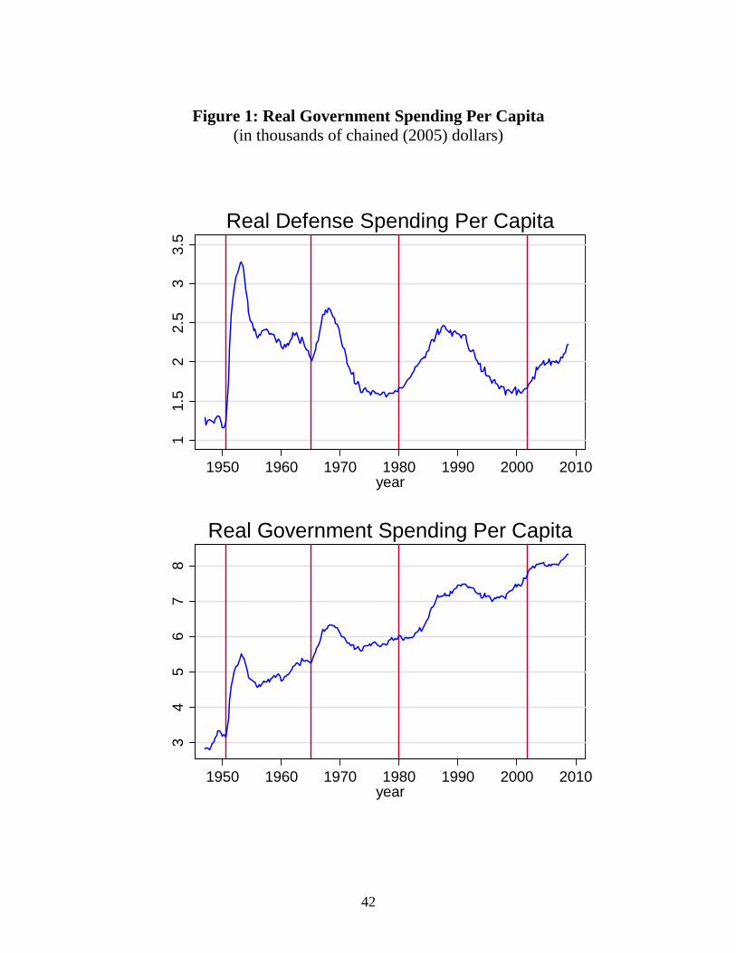
42

Figure 1: Real Government Spending Per Capita

(in thousands of chained (2005) dollars)

11.

52

2.5

33.

5

1950 1960 1970 1980 1990 2000 2010year

Real Defense Spending Per Capita

34

56

78

1950 1960 1970 1980 1990 2000 2010year

Real Government Spending Per Capita

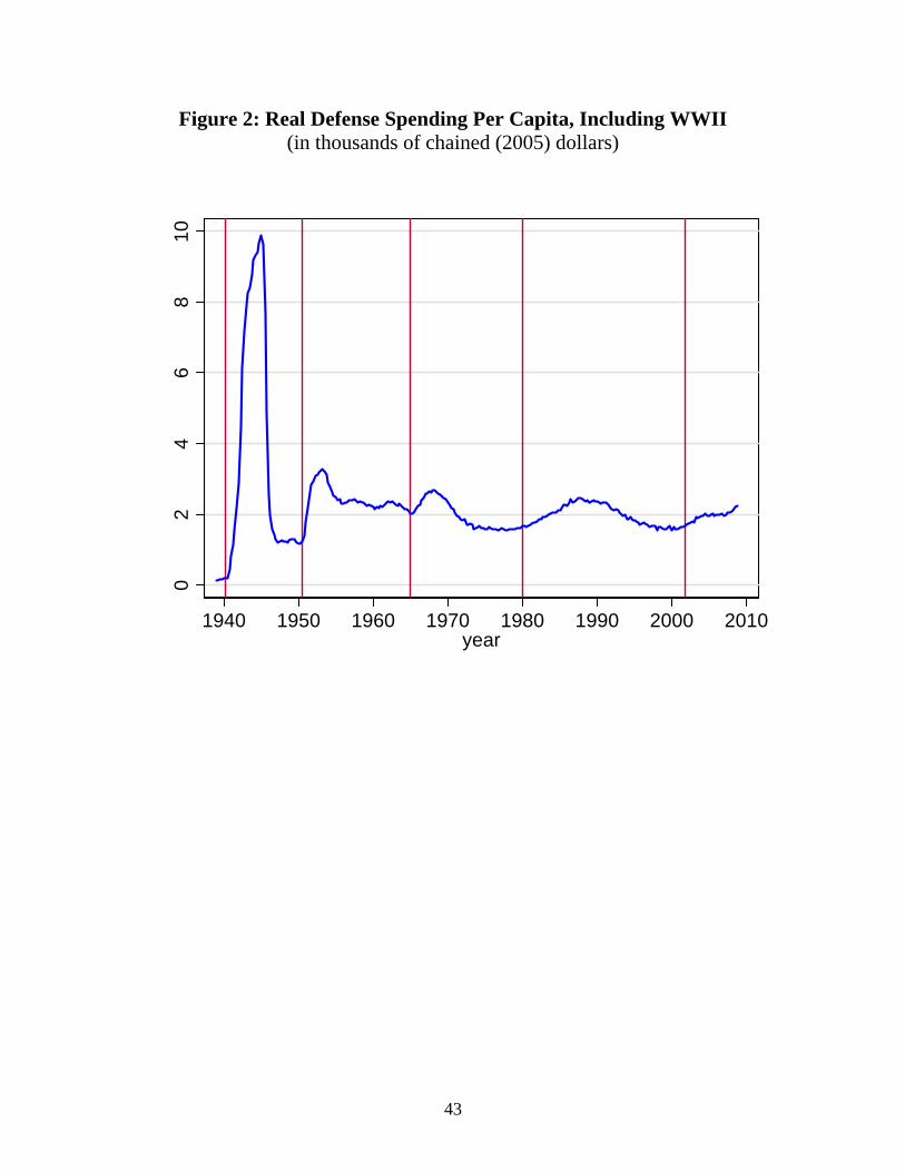
43

Figure 2: Real Defense Spending Per Capita, Including WWII (in thousands of chained (2005) dollars)

02

46

810

1940 1950 1960 1970 1980 1990 2000 2010year

44

Figure 3: Components of Government Spending Fraction of nominal GDP

0.0

5.1

.15

1950 1960 1970 1980 1990 2000 2010quarter

defense nondefense federalstate & local

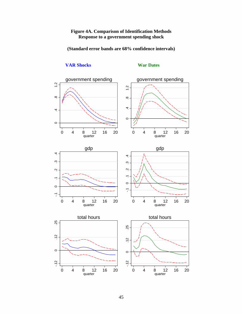
45

Figure 4A. Comparison of Identification Methods Response to a government spending shock

(Standard error bands are 68% confidence intervals)

VAR Shocks War Dates

0.4

.81.

2

0 4 8 12 16 20quarter

government spending

0.4

.81.

20 4 8 12 16 20

quarter

government spending

-.10

.1.2

.3.4

0 4 8 12 16 20quarter

gdp

-.10

.1.2

.3.4

0 4 8 12 16 20quarter

gdp

-.12

0.1

2.2

5

0 4 8 12 16 20quarter

total hours

-.12

0.1

2.2

5

0 4 8 12 16 20quarter

total hours

46

Figure 4B. Comparison of Identification Methods (continued) Response to a government spending shock

(Standard error bands are 68% confidence intervals)

VAR Shocks War Dates

-.2-.1

0.1

0 4 8 12 16 20quarter

consumption, ndur + serv

-.2-.1

0.1

0 4 8 12 16 20quarter

consumption, ndur + serv

-.9-.6

-.30

.3

0 4 8 12 16 20quarter

investment, nonres + res

-.9-.6

-.30

.3

0 4 8 12 16 20quarter

investment, nonres + res

-.18

-.12

-.06

0.0

6.1

2

0 4 8 12 16 20quarter

real wages

-.18

-.12

-.06

0.0

6.1

2

0 4 8 12 16 20quarter

real wages

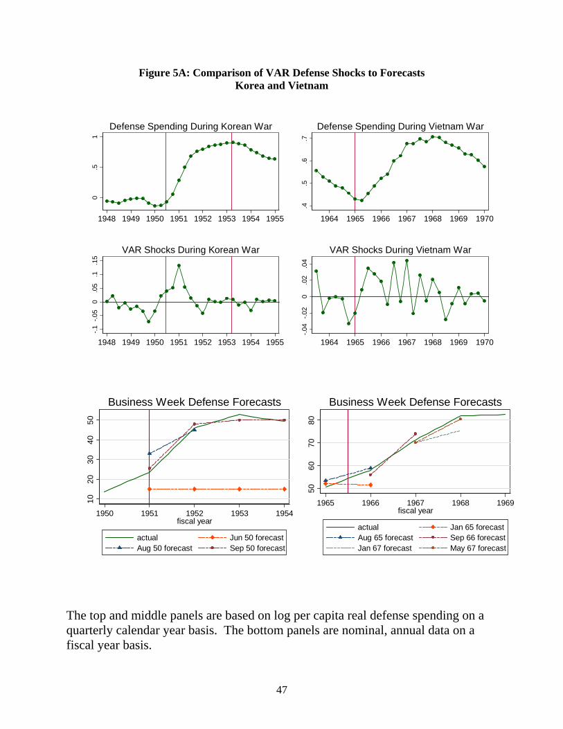
47

Figure 5A: Comparison of VAR Defense Shocks to Forecasts Korea and Vietnam

0

.51

1948 1949 1950 1951 1952 1953 1954 1955

Defense Spending During Korean War

.4.5

.6.7

1964 1965 1966 1967 1968 1969 1970

Defense Spending During Vietnam War

-.1-.0

50

.05

.1.1

5

1948 1949 1950 1951 1952 1953 1954 1955

VAR Shocks During Korean War

-.04

-.02

0.0

2.0

4

1964 1965 1966 1967 1968 1969 1970

VAR Shocks During Vietnam War

1020

3040

50

1950 1951 1952 1953 1954fiscal year

actual Jun 50 forecastAug 50 forecast Sep 50 forecast

Business Week Defense Forecasts

5060

7080

1965 1966 1967 1968 1969fiscal year

actual Jan 65 forecastAug 65 forecast Sep 66 forecastJan 67 forecast May 67 forecast

Business Week Defense Forecasts

The top and middle panels are based on log per capita real defense spending on a quarterly calendar year basis. The bottom panels are nominal, annual data on a fiscal year basis.

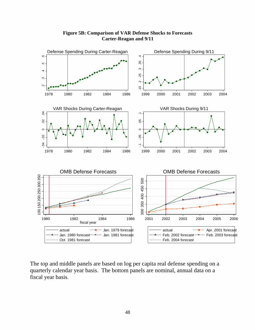
48

Figure 5B: Comparison of VAR Defense Shocks to Forecasts Carter-Reagan and 9/11

.2.3

.4.5

.6

1978 1980 1982 1984 1986

Defense Spending During Carter-Reagan

.15

.2.2

5.3

.35

.4

1999 2000 2001 2002 2003 2004

Defense Spending During 9/11

-.04

-.02

0.0

2.0

4

1978 1980 1982 1984 1986

VAR Shocks During Carter-Reagan

-.1-.0

50

.05

.1

1999 2000 2001 2002 2003 2004

VAR Shocks During 9/11

100

150

200

250

300

350

1980 1982 1984 1986fiscal year

actual Jan. 1979 forecastJan. 1980 forecast Jan. 1981 forecastOct. 1981 forecast

OMB Defense Forecasts

300

350

400

450

500

2001 2002 2003 2004 2005 2006

actual Apr. 2001 forecastFeb. 2002 forecast Feb. 2003 forecastFeb. 2004 forecast

OMB Defense Forecasts

The top and middle panels are based on log per capita real defense spending on a quarterly calendar year basis. The bottom panels are nominal, annual data on a fiscal year basis.

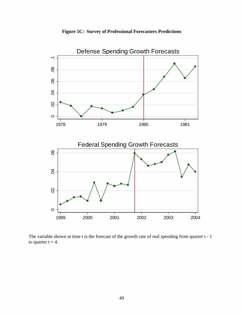
49

Figure 5C: Survey of Professional Forecasters Predictions

0.0

2.0

4.0

6.0

8.1

1978 1979 1980 1981

Defense Spending Growth Forecasts0

.02

.04

.06

1999 2000 2001 2002 2003 2004

Federal Spending Growth Forecasts

The variable shown at time t is the forecast of the growth rate of real spending from quarter t - 1 to quarter t + 4.

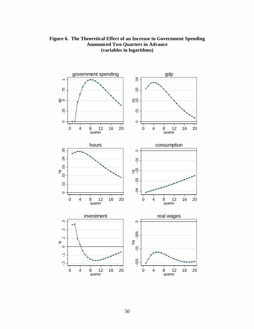
50

Figure 6. The Theoretical Effect of an Increase in Government Spending

Announced Two Quarters in Advance (variables in logarithms)

0

.25

.5.7

51

gg

0 4 8 12 16 20quarter

government spending

0.0

1.0

2.0

3.0

4yg

0 4 8 12 16 20quarter

gdp

0.0

1.0

2.0

3.0

4.0

5ng

0 4 8 12 16 20quarter

hours

-.04

-.03

-.02

-.01

0cg

0 4 8 12 16 20quarter

consumption

-.2-.1

0.1

.2.3

ig

0 4 8 12 16 20quarter

investment

-.015

-.01

-.005

0w

g

0 4 8 12 16 20quarter

real wages

51

Figure 7A. The Effect of Missing the Timing

Based on trivariate VARs on model simulations in which government spending changes are anticipated two quarter in advance

Shocks to actual Shocks to news government spending about government spending

0.4

.81.

2

0 4 8 12 16 20quarter

government spending

0.4

.81.

2

0 4 8 12 16 20quarter

government spending news

-.1-.0

50

.05

0 4 8 12 16 20quarter

gdp

-.1-.0

50

.05

0 4 8 12 16 20quarter

gdp

-.05

0.0

5.1

0 4 8 12 16 20quarter

hours

-.05

0.0

5.1

0 4 8 12 16 20quarter

hours

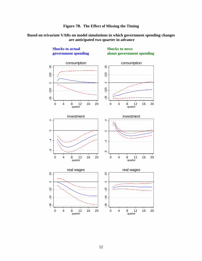
52

Figure 7B. The Effect of Missing the Timing

Based on trivariate VARs on model simulations in which government spending changes are anticipated two quarter in advance

Shocks to actual Shocks to news government spending about government spending

-.05

-.025

0.0

25.0

5

0 4 8 12 16 20quarter

consumption

-.05

-.025

0.0

25.0

50 4 8 12 16 20

quarter

consumption

-.8-.4

0.4

0 4 8 12 16 20quarter

investment

-.8-.4

0.4

0 4 8 12 16 20quarter

investment

-.06

-.04

-.02

0.0

2

0 4 8 12 16 20quarter

real wages

-.06

-.04

-.02

0.0

2

0 4 8 12 16 20quarter

real wages

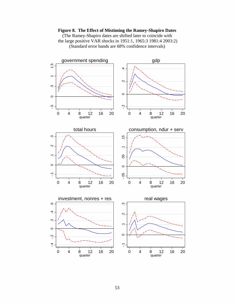
53

Figure 8. The Effect of Mistiming the Ramey-Shapiro Dates (The Ramey-Shapiro dates are shifted later to coincide with

the large positive VAR shocks in 1951:1, 1965:3 1981:4 2003:2) (Standard error bands are 68% confidence intervals)

-.50

.51

1.5

0 4 8 12 16 20quarter

government spending

-.20

.2.4

0 4 8 12 16 20quarter

gdp

-.10

.1.2

.3

0 4 8 12 16 20quarter

total hours-.0

50

.05

.1.1

5

0 4 8 12 16 20quarter

consumption, ndur + serv

-.4-.2

0.2

.4.6

0 4 8 12 16 20quarter

investment, nonres + res

-.10

.1.2

.3

0 4 8 12 16 20quarter

real wages

54

Figure 9. Defense News: PDV of Change in Spending as a % of GDP

-2

00

2040

6080

1940 1950 1960 1970 1980 1990 2000 2010year

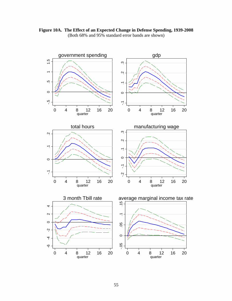
55

Figure 10A. The Effect of an Expected Change in Defense Spending, 1939-2008 (Both 68% and 95% standard error bands are shown)

-.50

.51

1.5

0 4 8 12 16 20quarter

government spending

-.10

.1.2

.3

0 4 8 12 16 20quarter

gdp-.1

0.1

.2

0 4 8 12 16 20quarter

total hours-.2

-.10

.1.2

.3

0 4 8 12 16 20quarter

manufacturing wage

-6-4

-20

24

0 4 8 12 16 20quarter

3 month Tbill rate

-.05

0.0

5.1

.15

0 4 8 12 16 20quarter

average marginal income tax rate

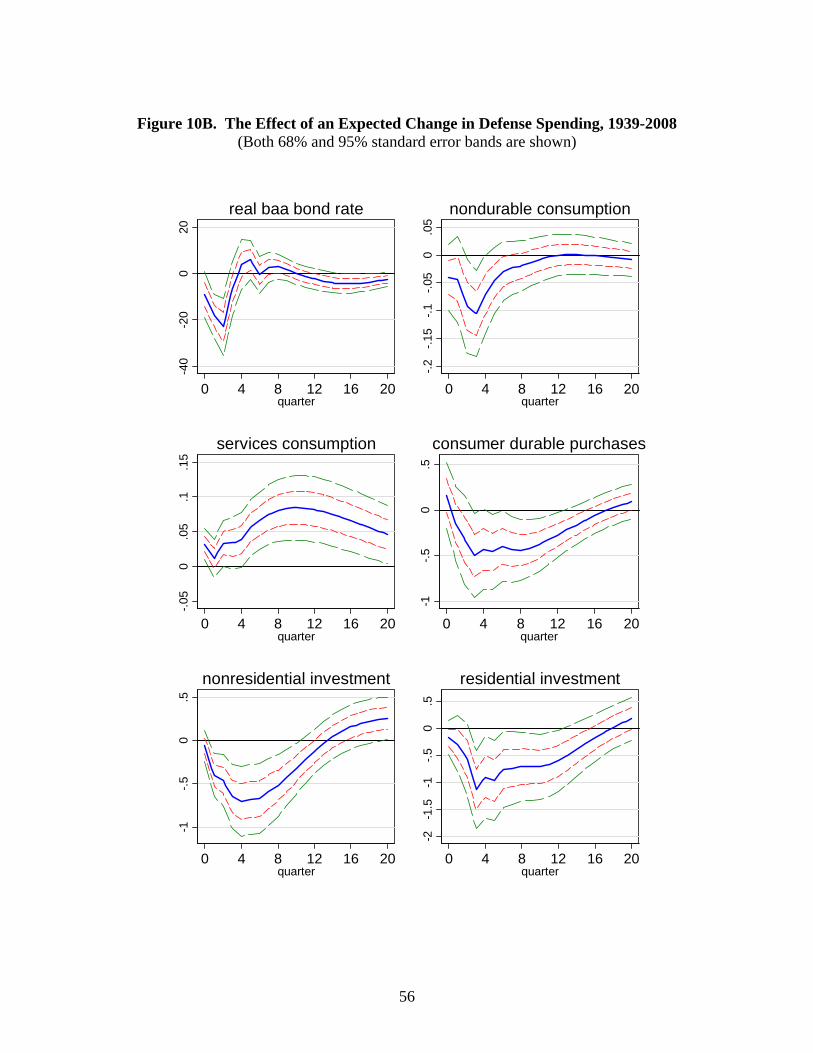
56

Figure 10B. The Effect of an Expected Change in Defense Spending, 1939-2008

(Both 68% and 95% standard error bands are shown)

-40

-20

020

0 4 8 12 16 20quarter

real baa bond rate

-.2-.1

5-.1

-.05

0.0

5

0 4 8 12 16 20quarter

nondurable consumption-.0

50

.05

.1.1

5

0 4 8 12 16 20quarter

services consumption-1

-.50

.5

0 4 8 12 16 20quarter

consumer durable purchases

-1-.5

0.5

0 4 8 12 16 20quarter

nonresidential investment

-2-1

.5-1

-.50

.5

0 4 8 12 16 20quarter

residential investment

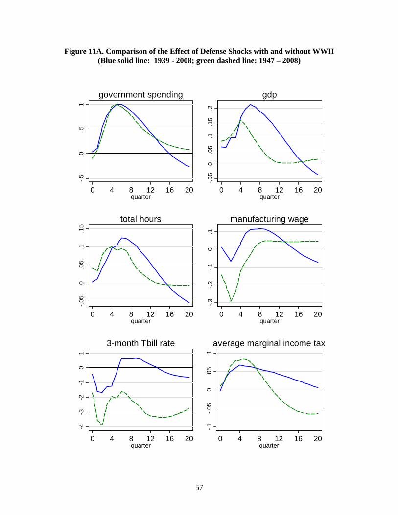
57

Figure 11A. Comparison of the Effect of Defense Shocks with and without WWII (Blue solid line: 1939 - 2008; green dashed line: 1947 – 2008)

-.5

0.5

1

0 4 8 12 16 20quarter

government spending

-.05

0.0

5.1

.15

.2

0 4 8 12 16 20quarter

gdp-.0

50

.05

.1.1

5

0 4 8 12 16 20quarter

total hours-.3

-.2-.1

0.1

0 4 8 12 16 20quarter

manufacturing wage

-4-3

-2-1

01

0 4 8 12 16 20quarter

3-month Tbill rate

-.1-.0

50

.05

.1

0 4 8 12 16 20quarter

average marginal income tax

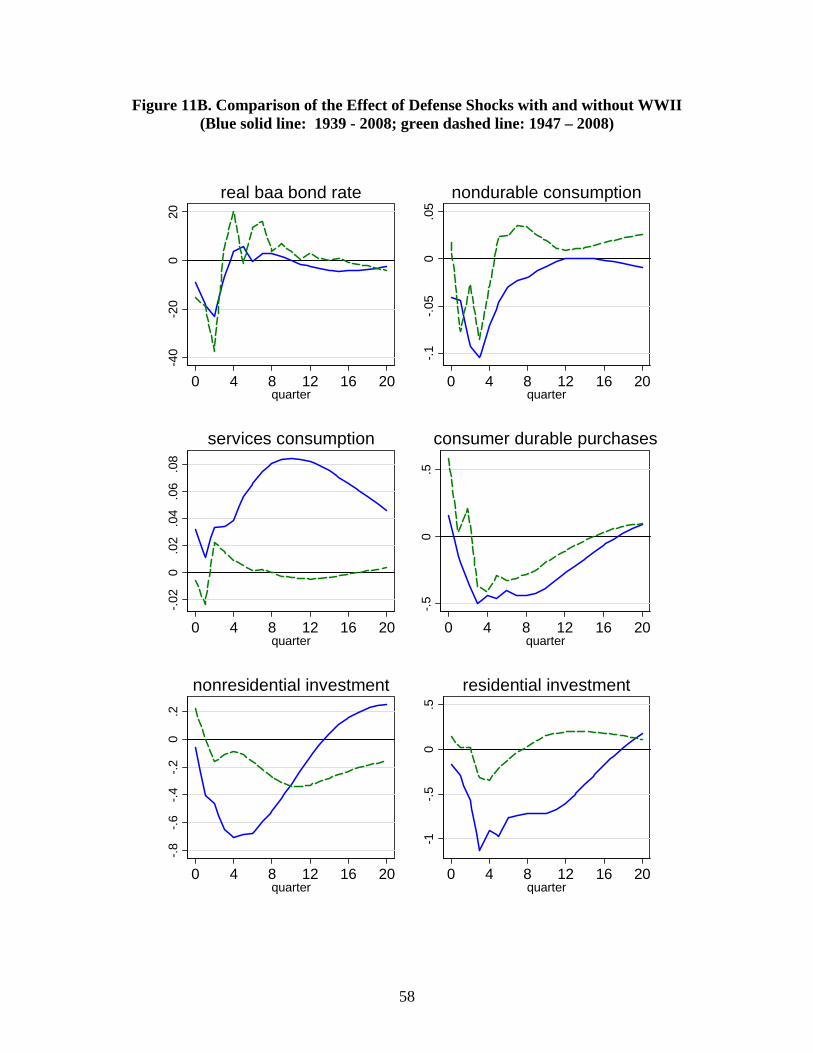
58

Figure 11B. Comparison of the Effect of Defense Shocks with and without WWII (Blue solid line: 1939 - 2008; green dashed line: 1947 – 2008)

-40

-20

020

0 4 8 12 16 20quarter

real baa bond rate

-.1-.0

50

.05

0 4 8 12 16 20quarter

nondurable consumption-.0

20

.02

.04

.06

.08

0 4 8 12 16 20quarter

services consumption-.5

0.5

0 4 8 12 16 20quarter

consumer durable purchases

-.8-.6

-.4-.2

0.2

0 4 8 12 16 20quarter

nonresidential investment

-1-.5

0.5

0 4 8 12 16 20quarter

residential investment

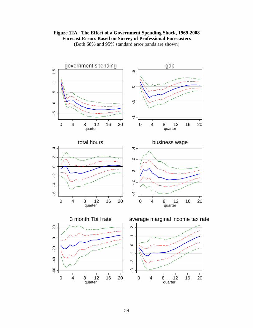
59

Figure 12A. The Effect of a Government Spending Shock, 1969-2008 Forecast Errors Based on Survey of Professional Forecasters

(Both 68% and 95% standard error bands are shown)

-.50

.51

1.5

0 4 8 12 16 20quarter

government spending

-1-.5

0.5

0 4 8 12 16 20quarter

gdp

-.6-.4

-.20

.2.4

0 4 8 12 16 20quarter

total hours

-.4-.2

0.2

.4

0 4 8 12 16 20quarter

business wage

-60

-40

-20

020

0 4 8 12 16 20quarter

3 month Tbill rate

-.3-.2

-.10

.1.2

0 4 8 12 16 20quarter

average marginal income tax rate

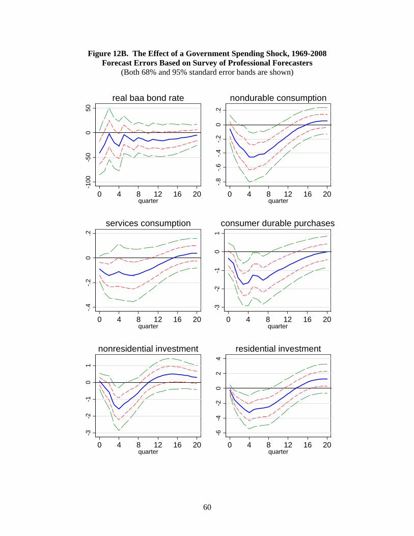
60

Figure 12B. The Effect of a Government Spending Shock, 1969-2008 Forecast Errors Based on Survey of Professional Forecasters

(Both 68% and 95% standard error bands are shown)

-100

-50

050

0 4 8 12 16 20quarter

real baa bond rate

-.8-.6

-.4-.2

0.2

0 4 8 12 16 20quarter

nondurable consumption-.4

-.20

.2

0 4 8 12 16 20quarter

services consumption-3

-2-1

01

0 4 8 12 16 20quarter

consumer durable purchases

-3-2

-10

1

0 4 8 12 16 20quarter

nonresidential investment

-6-4

-20

24

0 4 8 12 16 20quarter

residential investment