Identifying Government Spending Shocks: It’s All in the Timing

By

Valerie A. Ramey

University of California, San Diego National Bureau of Economic Research

First draft: July 2006 This draft: November 2007

This paper expands upon my March 2005 discussion at the Federal Reserve Bank of San Francisco conference “Fiscal and Monetary Policy.” I wish to thank Susanto Basu, Garey Ramey and participants at the 2006 NBER Summer Institute for helpful comments. I gratefully acknowledge financial support from National Science Foundation grant SES-0617219 through the NBER.

I. Introduction How does the economy respond to a rise in government purchases? Do consumption and

real wages rise or fall? The literature remains divided on this issue. VAR techniques in which

identification is achieved by assuming that government spending is predetermined within the

quarter typically find that a positive government spending shock raises not only GDP and hours,

but also consumption and the real wage (or labor productivity) (e.g. Rotemberg and Woodford

(1992), Blanchard and Perotti (2002), Fatás and Mihov (2001), Perotti (2004), Montford and

Uhlig (2005), and Galí, López-Salido, and Vallés (2006)). In contrast, analyses using the

Ramey-Shapiro (1998) “war dates” typically find that while government spending raises GDP

and hours, it lowers consumption and the real wage (e.g. Ramey and Shapiro (1998), Edelberg,

Eichenbaum, and Fisher (1999), Burnside, Eichenbaum, and Fisher (2004), and Cavallos

(2005)).

Whether government spending raises or lowers consumption and the real wage is crucial

for our understanding of how government spending affects GDP and hours. It is also important

for distinguishing macroeconomic models. Consider first the neoclassical approach, as

represented by papers such as Aiyagari, Christiano and Eichenbaum (1992) and Baxter and King

(1993). A permanent increase in government spending financed by nondistortionary means

creates a negative wealth effect for the representative household. The household optimally

responds by decreasing its consumption and increasing its labor supply. Output rises as a result.

The increased labor supply lowers the real wage and raises the marginal product of capital in the

short run. The rise in the marginal product of capital leads to more investment and capital

accumulation, which eventually brings the real wage back to its starting value. In the new

steady-state, consumption is lower and hours are higher. A temporary increase in government

1

spending in the neoclassical model has less impact on output because of the smaller wealth

effect. Depending on the persistence of the shock, investment can rise or fall. In the short run,

hours should still rise and consumption should still fall.1

The new Keynesian approach seeks to explain a rise in consumption, the real wage, and

productivity found in most VAR analyses. For example Rotemberg and Woodford (1992) and

Devereux, Head and Lapham (1996) propose models with oligopolistic (or monopolistic)

competition and increasing returns in order to explain the rise in real wages and productivity.

These models cannot, however, explain an increase in consumption. Galí, López-Salido, and

Vallés (2006) show that only an “ultra-Keynesian” model with sticky prices, “rule-of-thumb”

consumers, and off-the-labor-supply curve assumptions can explain how consumption and real

wages can rise when government spending increases. Their paper makes clear how many special

features the model must contain to explain the rise in consumption.

This paper reexamines the empirical evidence by comparing the two main empirical

approaches to estimating the effects of government spending: the VAR approach and the Ramey-

Shapiro narrative approach. After reviewing the set-up of both approaches and the basic results,

I show that a key difference appears to be in the timing. In particular, I show that the Ramey-

Shapiro dates Granger-cause the VAR shocks, but not vice versa. Thus, big increases in military

spending are anticipated several quarters before they actually occur. I show this is also true for

several notable cases of non-defense government spending changes. I then use a simple

neoclassical model to demonstrate that failing to account for the anticipation effect can explain

all of the differences in the empirical results of the two approaches.

1 Adding distortionary taxes or government spending that substitutes for private consumption or capital adds additional complications. See Baxter and King (1993) and Burnside, Eichenbaum, and Fisher (2004) for discussions of these complications.

2

Nevertheless, concerns have been raised about the Ramey-Shapiro dates because they are

so few (e.g. Perotti (2007)). I thus construct a new measure of exogenous defense shocks using

narrative evidence on expectations and including more increases driven by political events. This

new measure yields much the same results as the original Ramey-Shapiro dates.

II. Fluctuations in Government Spending in the Post-WWII Era

This section reviews the trends and fluctuations in the components of government

spending. One key difference between the two approaches is whether the shocks identified are

shocks to all of government spending or to defense spending alone. As we will see, this may

make a difference.

Figure 1 shows the paths of real defense spending per capita and total real government

spending per capita in the post-WWII era.2 The lines represent the Ramey-Shapiro (1998) dates,

including the Korean War, the Vietnam War, and the Soviet invasion of Afghanistan, augmented

by 9/11. These dates will be reviewed in detail below. The major movements in defense

spending all come following one of the four military dates. Korea is obviously the most

important, but the other three are also quite noticeable. There are also two minor blips in the

second half of the 1950s and early 1960.

Looking at the bottom graph in Figure 1, we see that total government spending shows a

significant upward trend over time. Nevertheless, the defense buildups are still distinguishable

after the four dates. The impact of the Soviet invasion of Afghanistan has a delayed effect on

total government spending, because nondefense spending fell.

2 Per capita variables are created using the entire population, including armed forces overseas.

3

Figure 2 shows defense spending, nondefense federal spending, and state and local

spending as a fraction of GDP (in nominal terms). The graph shows that relative to the size of

the economy, each military buildup has become smaller over time. Federal nondefense spending

is a minor part of government spending, hovering around two to three percent of GDP. In

contrast, state and local spending has risen from around five percent of GDP in 1947 to over

twelve percent of GDP now. Since state and local spending is driven in large part by cyclical

fluctuations in state revenues, it is not clear that aggregate VARs are very good at capturing

shocks to this type of spending. For example, California dramatically increased its spending on

K-12 education when its tax revenues surged from the dot-com boom in the second half of the

1990s.

The graphs suggest that defense spending is a major part of the variation in government

spending around trend. To quantify the importance of defense spending, I estimate a variance

decomposition of government spending using a simple VAR. I include the log of real total

government spending, defense spending and either state and local spending or federal

nondefense. All variables are in real per capita terms. Four lags and a trend are included in the

VAR. Table 1 shows the variance decomposition of total government spending at various

horizons for different orderings of the variables. The table shows that no matter the ordering,

shocks to defense spending account for 80 to 90 percent of the forecast error variance of total

government spending for horizons of four to twenty quarters. Thus, the variance decomposition

suggests that shocks to defense spending accounts for almost all of the unforeseen changes in

total government spending.

What kind of spending constitutes nondefense spending? Figure 3 shows annual

spending for some key functions, as a percent of total government spending. Spending by

4

function is available annually only since 1959. The category of education, public order (which

includes police, courts and prisons), and transportation expenditures has increased from 30

percent of total government spending to around 50 percent.

The standard VAR approach includes shocks to this type of spending in its analysis (e.g.

Blanchard and Perotti (2002)). Such an inclusion is questionable for several reasons. First, the

biggest part of this category, education, is driven in large part by demographic changes, which

can have many other effects on the economy. Second, these types of expenditures would be

expected to have a positive effect on productivity and hence would have a different effect than

government spending that has no direct production function impacts. As Baxter and King (1993)

make clear, the typically neoclassical predictions about the effects of government spending

change completely when government spending is “productive.” Even the “other” category

shown has questionable impacts, since it includes “other economic activities” such as spending

on natural resources, housing and health. Thus, including these categories in spending shocks is

not the best way to test the neoclassical model versus the Keynesian model.

Some of the analyses, such as Eichenbaum and Fisher (2005) and Perotti (2007), have

tried to address this issue by using only “government consumption” and excluding “government

investment.” Unfortunately, this National Income and Product Account distinction does not

help. As the footnotes to the NIPA tables state: “Government consumption expenditures are

services (such as education and national defense) produced by government that are valued at

their cost of production….Gross government investment consists of general government and

government enterprise expenditures for fixed assets.” Thus, since teacher salaries are the bulk of

education spending, they would be counted as “government consumption.”

5

In sum, three conclusions emerge from this review of the data. First, while nondefense

spending accounts for most of the trend in government spending, fluctuations in defense

spending account for almost all of the fluctuations in total government spending relative to trend.

Second, most nondefense spending is done by state and local governments, not by the federal

government, so it is not clear that aggregate VARs are very good at capturing shocks to this type

of spending. Third, much of nondefense expenditures consists of spending that may impact the

productivity of the economy, and thus should not be included in analyses of the pure effects of

government spending.

III. Identifying Government Spending Shocks: VAR vs. Narrative Approaches

A. The VAR Approach

Blanchard and Perotti (2002) have perhaps the most careful and comprehensive approach

to estimating fiscal shocks using VARs. To identify shocks, they first incorporate institutional

information on taxes, transfers, and spending to set parameters, and then estimate the VAR.

Their basic framework is as follows:

ttt UYqLAY += −1),(

where Yt consists of quarterly real per capita taxes, government spending, and GDP. Although

the contemporaneous relationship between taxes and GDP turns out to be complicated, they find

that government spending does not respond to GDP or taxes contemporaneously. Thus, their

identification of government spending shocks is identical to a Choleski decomposition in which

government spending is ordered before the other variables. When they augment the system to

include consumption, they find that consumption rises in response to a positive government

spending shock. Galí et al (2006) use this basic identification method in their study which

6

focuses only on government spending shocks and not taxes. They estimate a VAR with

additional variables of interest, such as real wages, and order government spending first. Perotti

(2007) uses this identification method to study a system with seven variables. 3

B. The Ramey-Shapiro Narrative Approach

In contrast, Ramey and Shapiro (1998) use a narrative approach to identify shocks to

government spending. Because of their concern that many shocks identified from a VAR are

simply anticipated changes in government spending, they focus only on episodes where Business

Week suddenly began to forecast large rises in defense spending induced by major political

events that were unrelated to the state of the U.S. economy. The three episodes identified by

Ramey and Shapiro were as follows:

Korean War

On June 25, 1950 the North Korean army launched a surprise invasion of South Korea,

and on June 30, 1950 the U.S. Joint Chiefs of Staff unilaterally directed General MacArthur to

commit ground, air, and naval forces. In the July 1, 1950 issue, Business Week wrote: “We are

no longer in a peacetime economy. Even if the Communists should back down in Korea, we

have had a warning of what can happen any time at all or in any of the Asiatic nations bordering

on the USSR. The answer will be more money for arms.” (p. 9). After early UN victories,

Business Week in October 1950 predicted a quick end to hostilities in Korea, but a continuing

defense spending increase. It predicted a somewhat faster pace of spending after China entered

the war on November 9, 1950, but pointed out that it would take at least six months to translate

defense programs into men and material. The December 2, 1950 issue predicted a bigger war, 3 See the references listed in the introduction to see the various permutations on this basic set-up.

7

also stating: “It will be mid-year before defense plans are firm, maybe longer … Then it will take

at least six months to translate the program into men and material.” (p. 16). Many articles in late

1950 and in 1951 discussed Pentagon bottlenecks in awarding defense contracts.

The Vietnam War

Despite the military coup that overthrew Diem on November 1, 1963, Business Week

was still talking about defense cuts for the next year (November 2, 1963, p. 38; July 11, 1964, p.

86). Even the Gulf of Tonkin incident on August 2, 1964 brought no forecasts of increases in

defense spending. However, after the February 7, 1965 attack on the U.S. Army barracks,

Johnson ordered air strikes against military targets in North Vietnam. The February 13, 1965,

Business Week said that this action was “a fateful point of no return” in the war in Vietnam.

Fighting escalated in the spring and expenses increased beyond initial estimates. In July 1965,

Johnson told the nation “This is really war” and doubled draft quotas. On December 4, 1965,

Business Week said that the price tag for the Vietnam War was drastically marked up that week

and that there was no end in sight.

The Carter-Reagan Buildup

The long decline in defense spending began to turn around slightly when Carter promised

NATO that the US would increase defense spending by an inflation-adjusted three percent a

year. The Soviet invasion of Afghanistan on December 24, 1979 led to a significant turnaround

in U.S. defense policy. The event was particularly worrisome because some believed it was a

possible precursor to actions against Persian Gulf oil countries. The January 21, 1980 Business

Week (p.78) printed an article entitled “A New Cold War Economy” in which it forecasted a

8

significant and prolonged increase in defense spending. It declared that Détente was in

shambles. It predicted an extra $96 billion more in defense spending spread over a five to seven

year period. Reagan was elected in November 1980 and promised to increase defense spending

somewhat. In the spring of 1981, Reagan proposed to increase defense spending by $181 billion

over the next five years.

These dates were based on data up through 1998. Owing to recent events, I now add the

following date to these war dates:

9/11

On September 11, 2001, terrorists struck the World Trade Center and the Pentagon. On

October 1, 2001, Business Week forecasted that the balance between private and public sectors

would shift, and that spending restraints were going “out the window.” In this case, though, it

was clear that some of the increased spending they were discussing was not defense, but rather

industry bailouts and the like. To recall the timing of key subsequent events, the U.S. invaded

Afghanistan soon after 9/11. It invaded Iraq on March 20, 2003.

C. Comparison of Impulse Response Functions

Consider now a comparison of the effects of government spending increases based on the

two identification methods. In both instances, I use a VAR similar to the one used recently by

Perotti (2007) with a few modifications of variable definitions. The VAR consists of the log real

per capita quantities of total government spending, GDP, total hours worked, nondurable plus

services consumption, and private fixed investment, as well as Perotti’s version of the Barro-

Sahasakul tax rate, the log of nominal compensation in private business divided by the deflator in

9

private business. I use total hours worked instead of private hours worked based on Cavallo’s

(2005) work showing that a significant portion of rises in government spending consists of

increases in the government payroll. Also, note that I use a product wage rather than a

consumption wage. Ramey and Shapiro (1998) show both theoretically and empirically why it is

the product wage that should be used when trying to distinguish models of government spending.

Defense spending tends to be concentrated in a few industries, such as manufactured goods.

Ramey and Shapiro show that the relative price of manufactured goods rise significantly during a

defense buildup. Thus, product wages in the expanding industries can fall at the same time that

the consumption wage is unchanged or rising.4

Both VARs are specified in levels, with a time trend and four lags included. Because the

tax rate series only extends to 2003:4, I use quarterly data from 1947:1 to 2003:4. In the VAR

identification, the government spending shock is identified by a Choleski decomposition in

which government spending is ordered first. In the war dates identification, the current value

and four lags of a dummy variable with the military date are also included. The military date

takes a value of unity in 1950:3, 1965:1, 1980:1, and 2001:3.5 I compare the effects of shocks

lead government spending to peak at unity in both specifications.

Figures 4A and 4B show the impulse response functions. Following the government

spending VAR literature (e.g. Galí et al (2007) and Perotti (2007)) , the standard error bands are

68% bands, based on bootstrap standard errors. This standard of significance is far below the

standards in other literatures, but I conform in order that the graphs be clearer. Also, more

parsimonious representations tend to give similar point estimates with smaller standard errors, so

4 The main reason that Rotemberg and Woodford (1992) find that real wages increase is that they construct their real wage by dividing the wage in manufacturing by the implicit price deflator. Ramey and Shapiro show that the wage in manufacturing divided by the price index for manufacturing falls during a defense buildup. 5 Burnside, Eichenbaum and Fisher (2004) allow the value of the dummy variable to differ across episodes according to the amount that government spending increase. They obtain very similar results.

10

the results are often significant at conventional levels (e.g. Ramey-Shapiro (1998) and Edelberg

et al (1999).

The first column shows the results from the VAR identification and the second column

shows the results from the war dates identification. Figure 4A shows the effects on government

spending, GDP, and hours. The results are qualitatively consistent across the two identification

schemes for these three variables. By construction, total government spending rises by the same

amount, although the peak occurs several quarters earlier in the VAR identification. This is the

first indication that a key difference between the two methods is timing. GDP rises in both

cases, but its rise is much greater in the case of the war dates identification. Hours rise slightly

in the VAR identification, but much more strongly in the war dates identification. A comparison

of the output and hours response shows that productivity rises slightly in both specifications.

Figure 4B shows the cases in which the two identification schemes differ in their

implications. The VAR identification scheme implies that government spending shocks raise

consumption, lower investment for two years, and raise the real wage. In contrast, the war dates

identification scheme implies that government spending shocks lower consumption, raise

investment for a few quarters before lowering it, and lower the real wage.

Overall, these two approaches give diametrically opposed answers with regard to some

key variables. The next section presents empirical evidence and a theoretical argument that can

explain the differences.

IV. The Importance of Timing

A concern with the VAR identification scheme is that some of what it classifies as

“shocks” to government spending may well be anticipated. Indeed, Blanchard and Perotti (2002)

11

worried about this very issue, and devoted Section VIII of their paper to analyzing it. To test for

the problem of anticipated policy, they included future values of the estimated shocks to

determine whether they affected the results. They found that the response of output was greater

once they allowed for anticipation effects (see Figure VII). Unfortunately, they did not show

how the responses of consumption or real wages were affected. Perotti (2004) approached the

anticipation problem by testing whether OECD forecasts of government spending predicted his

estimated government spending shocks. For the most part, he found that they did not predict the

shocks.

In the next subsection, I show that the war dates do predict the VAR government

spending shocks. I also show how in each war episode, the VAR shocks are positive several

quarters after Business Week started forecasting increases in defense spending. In the second

subsection, I present simulations from a simple theoretical model that shows how the difference

in timing can explain most of the differences in results. In the final subsection, I show that

delaying the timing of the Ramey-Shapiro dates produces the Keynesian results.

A. Empirical Evidence on Timing Lags

To compare the timing of war dates versus VAR-identified shocks, I estimate shocks

using the VAR discussed above except with defense spending rather than total government

spending as the key variable. I then plot those shocks around the war dates.

Figure 5 shows the path of log per capita real defense spending and the series of

identified shocks. Consider first the Korean War. The first vertical line shows the date when the

Korea War started. The second vertical line indicates when the armistice was signed in July

1953. According to the VAR estimates, shown in the graph below, there was a series of three

12

large positive shocks to defense in 1950:4, 1950:1, and 1950:2. However, as Business Week

made clear, the path of defense spending during these three quarters was anticipated as of July

1950. Moreover, the negative shock to defense estimated in the first quarter of 1952 corresponds

to the decision to spread out defense spending over a longer period. It is also interesting to note

that while Business Week was predicting a future decline in defense spending as early as April

1953 when a truce seemed imminent, the VAR records a negative defense spending shock late in

the first quarter of 1954.

Vietnam shows a similar pattern in that the war date predates a series of positive shocks

from the VAR. As I will discuss below, some of the positive shocks in 1965 may indeed have

been unanticipated increases in spending. According to Business Week, estimates of the cost of

the Vietnam War rose significantly in the months after the initial air strikes in February 1965.

However, the VAR method shows continuing positive shocks through 1968.

The Carter-Reagan build-up shows many positive shocks through 1985. As I will discuss

below, this build-up may have had several surprises, such as Reagan’s landslide election in

November 1980 and his initial defense budgets proposed in early 1981. On the other hand, much

of the spending that occurred from 1982 to 1985 was scheduled several years before.

After 9/11 the VAR implies virtually no shocks until the second quarter of 2003. Yet

many were predicting increases in defense spending well before this. While Iraq turned out to

cost much more than the Administration initially forecast, many did not believe those forecasts.

Thus, it appears that the VAR might be labeling as “shocks” changes in defense spending

that were forecastable. To test this hypothesis, I perform Granger causality tests between the war

dates and VAR-based defense and total government spending shocks. Table 2 shows the results.

13

The evidence is very clear: the war dates Granger-cause the VAR shocks but the VAR shocks

do not Granger-cause the war dates.

One should be clear that this is not an issue only with defense spending. Consider the

interstate highway program. In early 1956, Business Week was predicting that the “fight over

highway building will be drawn out.” By May 5, 1956, Business Week thought that the highway

construction bill was a sure bet. It fact it passed in June 1956. However, the multi-billion dollar

program was intended to stretch out over 13 years. It is difficult to see how a VAR could

accurately reflect this program. Another example is schools for the Baby Boom children.

Obviously, the demand for schools is known several years in advance. Between 1949 and 1969,

real per capita spending on public elementary and secondary education increased 300%.6 Thus, a

significant portion of non-defense spending is known months, if not years, in advance.

B. The Importance of Timing in a Theoretical Model

To see how important anticipation effects can be, consider the following calibrated

quarterly neoclassical model:

tKtItK

tGtItCtY

tNttCU

tKtNtZtY

)023.01(1

)1log()log(

33.067.0)(

−+=+

++=

−⋅+=

=

ϕ

6 The nominal figures on expenditures are from the Digest of Education Statistics. I used the GDP deflator to convert to real.

14

Y is output, N is labor, K is capital, C is consumption, I is investment, and G is government

purchases. Government purchases are financed with nondistortionary taxes. Households

maximize the present discounted value of utility U with discount factor β = 0.99.

The driving processes are calibrated as follows:

2

321

1

1

ln

028.0,ln25.0ln18.0ln4.1constant ln

008.0,ln95.ln

01.0,ln95.ln

−

−−−

−

−

=

=+−−+=

=+⋅=

=+⋅=

tt

egttttt

ettt

ezttt

GFG

egGFGFGFGF

e

ezZZ

σ

σϕϕϕ

σ

ϕ

The calibration for the technology shock is standard. The calibrations for the marginal rate of

substitution shock and the government spending shock are based on my estimates. “GF” is the

forecast of government spending whereas G is actual government spending. This specification

allows agents to know the shock to actual government spending two quarters in advance.

Figure 6 shows the impulse response functions from this model. News becomes available

in quarter 0, but government spending does not start to increase until quarter two. In contrast,

output, hours, consumption, investment and real wages all jump in quarter 0 when the news

arrives. Output and hours rise immediately, while consumption and real wages fall immediately.

Interestingly, investment rises for several quarters before it falls.

Looking at these graphs, one wonders what happens in a VAR if one identifies the

government spending shock from when government spending actually changes. To study this

15

effect, I simulate data from this model and run two types of bivariate VARs. In the “faulty

timing” VARs, I use actual government spending and the variable of interest. In the “true

timing” VARs, I use the news (“GF”) and the variable of interest. In all cases, I order the

government spending variable first.

Figures 7A and 7B show the results. The faulty timing VARs are shown in left column

and the true timing VARs are shown in the right column. The patterns across the two columns

are strikingly similar to the patterns across the VARs on real data using the two methods shown

in Figures 4A and 4B. In particular, the faulty timing finds a much smaller response of GDP

than the true timing, just as the standard VAR identification method finds a smaller response

than the Ramey-Shapiro military dates. The same is true of hours. In Figure 7B, we see that the

faulty timing VAR leads to rises in consumption and real wages, whereas the true timing VAR

leads to falls in consumption and real wages. The problem with the faulty timing VAR is that

they catch the variables after they have already had an initial response to the news.

One could modify the theoretical model to incorporate elements such as habit persistence

in consumption and/or adjustment cost in investment. In this case, the true responses would be

more dragged out and missing the timing by two quarters would have a somewhat smaller effect.

However, missing the timing by a few quarters would have changed the impulse responses just

as they did in the previous example.

C. Would Delaying the Ramey-Shapiro Dates Lead to Keynesian Results?

If the theoretical argument of the last section applies to the current situation, then

delaying the timing of the Ramey-Shapiro dates should results in VAR-type Keynesian results.7

7 This idea was suggested to me by Susanto Basu.

16

To investigate this possibility, I shifted the four military dates to correspond with the first big

positive shock from the VAR analysis. Thus, instead of using the original dates of 1950:3,

1965:1, 1980:1, and 2001:3, I used 1951:1, 1965:3, 1980:4, and 2003:2.

Figure 8 shows the results. As predicted by the theory, the delayed Ramey-Shapiro dates

now lead to rises in consumption and the real wage, similarly to the shocks from the standard

VARs. Thus, the heart of the difference between the two results appears to be the VAR’s delay

in identifying the shocks.

Alternatively, one could try to estimate the VAR and allow future identified shocks to

have an effect. Blanchard and Perotti (2002) did this for output, but never looked at the effects

on consumption or wages. Based on an earlier draft of my paper, Tenhofen and Wolff (2007)

analyze such a VAR for consumption and find that when the VAR timing changes, positive

shocks to defense spending lead consumption to fall.

Thus, all of the empirical and theoretical evidence points to timing as being key to the

difference between the standard VAR approach and the Ramey-Shapiro approach. The fact that

the Ramey-Shapiro dates Granger-cause the VAR shocks suggests that the VARs are not

capturing the timing of the news. The theoretical analysis shows that timing is crucial in

determining the response of the economy to news about increases in government spending.

V. A New Measure of Narrative Shocks

The last sections have presented evidence that the narrative approach is superior to the

standard VAR approach in isolating the timing of government shocks. Nevertheless, one might

be concerned with the original Ramey-Shapiro dates because they are so few. Also, several

17

researchers have felt it was better to scale the original dummy variables (e.g. Eichenbaum and

Fisher (2005)), but often the scaling depends on ex-post outcomes.

In order to create a measure of defense shocks that is richer and overcomes some of these

problems, I returned to the narrative record in order to isolate more events that led the press to

forecast increases in defense spending. Most was based on Business Week, but a few other

sources such as the New York Times, were used as well. I only used government records, such as

the U.S. Budget and the Congressional Budget Office forecasts, to confirm some numbers from

the press. These latter documents were not produced at high enough frequency to ensure that the

timing was correct.

Table 3 shows the list of events and the magnitudes assigned to them. The magnitudes

are based on estimates of the increase in spending over the next several years. Because the press

never gives present values, I do not use them either. The estimates are very rough and many are

based on judgment calls, but it is hoped that they are at least more informative than just assigning

unity to each event. Because many of the values of the new series are zero or negative, one

cannot use logarithms in the analysis. I therefore scale them by the level of nominal defense

spending the previous period.

Table 4 shows how these shocks compare to the original Ramey-Shapiro dates in

predicting defense spending. The first row shows that the new series has substantial additional

explanatory power for defense spending over and above its own lags. Interestingly, the new

series is not as good at predicting GDP as the original Ramey-Shapiro series. On the other hand,

it is slightly better at predicting consumption.

18

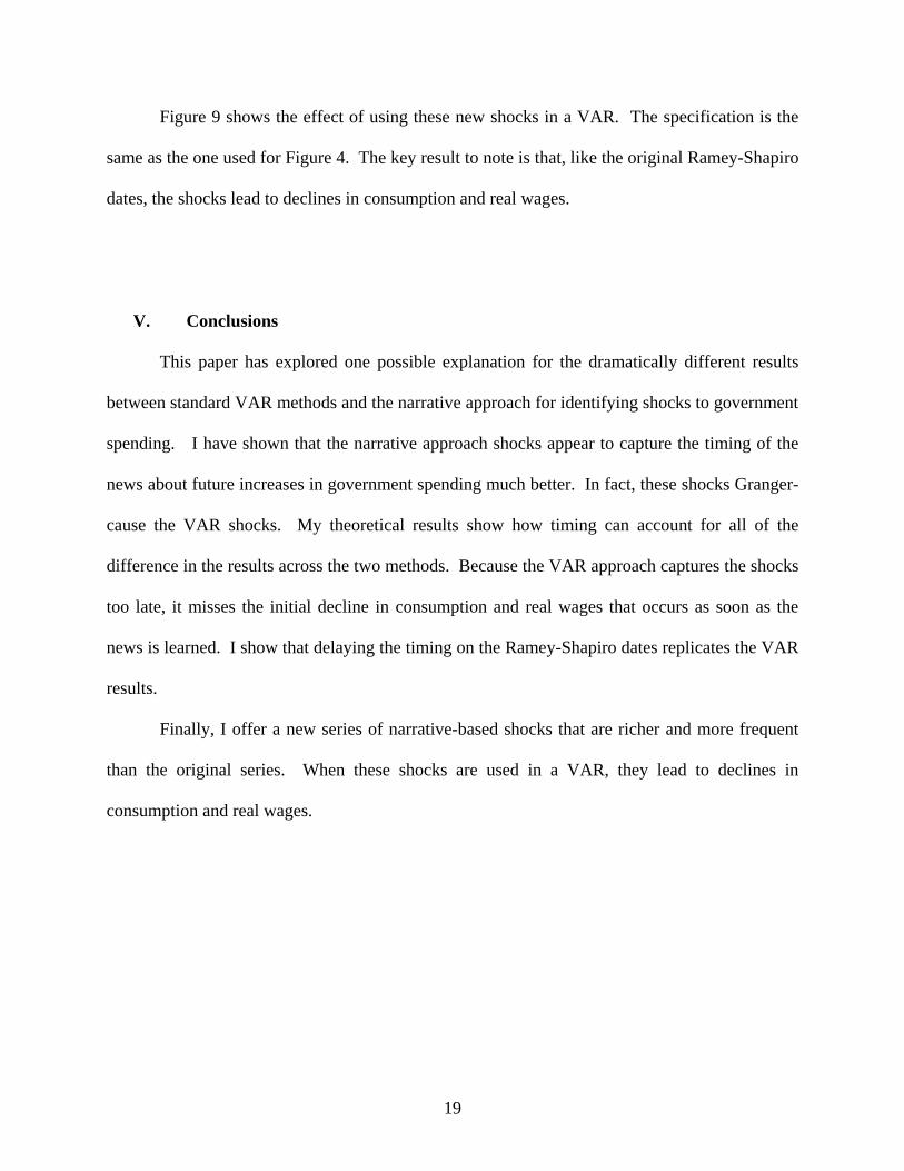
Figure 9 shows the effect of using these new shocks in a VAR. The specification is the

same as the one used for Figure 4. The key result to note is that, like the original Ramey-Shapiro

dates, the shocks lead to declines in consumption and real wages.

V. Conclusions

This paper has explored one possible explanation for the dramatically different results

between standard VAR methods and the narrative approach for identifying shocks to government

spending. I have shown that the narrative approach shocks appear to capture the timing of the

news about future increases in government spending much better. In fact, these shocks Granger-

cause the VAR shocks. My theoretical results show how timing can account for all of the

difference in the results across the two methods. Because the VAR approach captures the shocks

too late, it misses the initial decline in consumption and real wages that occurs as soon as the

news is learned. I show that delaying the timing on the Ramey-Shapiro dates replicates the VAR

results.

Finally, I offer a new series of narrative-based shocks that are richer and more frequent

than the original series. When these shocks are used in a VAR, they lead to declines in

consumption and real wages.

19

References

Aiyagari, Rao, Laurence Christiano and Martin Eichenbaum, “The Output, Employment and Interest Rate Effects of Government Consumption.” Journal of Monetary Economics 30 (1992), pp. 73–86.

Baxter, Marianne and Robert G. King, “Fiscal Policy in General Equilibrium,” American

Economic Review 83 (1993), pp. 315–334. Blanchard, Olivier and Roberto Perotti, “An Empirical Characterization of the Dynamic Effects

of Changes in Government Spending and Taxes on Output,” Quarterly Journal of Economics (November 2002): 1329-1368.

Burnside, Craig, Martin Eichenbaum, and Jonas Fisher, “Fiscal Shocks and their Consequences,”

Journal of Economic Theory 115 (2004): 89-117. Devereux, Michael, A. C. Head and M. Lapham, “Monopolistic Competition, Increasing

Returns, and the Effects of Government Spending,” Journal of Money, Credit, and Banking 28 (1996), pp. 233–254.

Edelberg, Wendy, Martin Eichenbaum and Jonas D. M. Fisher, “Understanding the Effects of a

Shock to Government Purchases,” Review of Economic Dynamics 2 (January 1999): 166-206.

Gali, Jordi, J. David López-Salido, and Javier Vallés, “Understanding the Effects of Government

Spending on Consumption,” Journal of the European Economic Association, 5 (March 2007): 227-270.

Perotti, Roberto, “In Search of the Transmission Mechanism of Fiscal Policy,” forthcoming

NBER Annual 2007. Ramey, Valerie A. and Matthew Shapiro, “Costly Capital Reallocation and the Effects of

Government Spending,” Carnegie Rochester Conference on Public Policy (1997). Rotemberg, Julio and Woodford, Michael, “Oligopolistic Pricing and the Effects of Aggregate

Demand on Economic Activity,” Journal of Political Economy 100 (1992), pp. 1153–1297.

Tenhofen, Jorn and Guntram Wolff, “Does Anticipation of Government Spending Matter?

Evidence from an Expectations Augmented VAR,” Deutsche Bundesbank working paper, 2007.

20

Table 1. Variance Decomposition of Government Spending Percent Explained by Shocks to Defense Spending

VAR ordering

Horizon (in quarters)

Defense, state & local, total

State & local, defense, total

Federal nondefense, defense, total

1 57 57 66 4 85 86 83 10 92 92 91 20 91 91 92

Based on estimated VARs with four lags and a time trend. All variables are log real per capita.

Table 2. Granger Causality Tests

Hypothesis Tests p-value Defense shocks H0: War dates do not Granger-cause VAR shocks 0.006 H0: VAR shocks do not Granger-cause war dates 0.334 Government spending shocks Do War dates Granger cause VAR shocks? 0.026 Do VAR shocks Granger cause War dates? 0.159 VAR shocks were estimated by regressing the log of the variable of interest on 4 lags of itself, the Barro-Sahasakul tax rate, log real per capita GDP, log real per capita nondurable plus services consumption, log real per capita private fixed investment, log real per capita total hours worked, and log compensation in private business divided by the deflator for private business. The test regressed the second variable on 4 lags of the first variable. The war dates are variables that take a value of unity at 1950:3, 1965:1, 1980:1, 2001:3.

21

Table 3. New Defense Shocks based on the Narrative Approach

Political Events Date of shock

Amount in billions over next several years

Britain asks US to take over defense in Europe, Greek crisis 1947q2 0.4Marshall Plan 1947q3 13Rearmament, Berlin Airlift 1948q2 4

Soviet actions lead to escalation. 1950q2 4

N. Korea invades S. Korea 1950q3 53China invades Oct. 19, 1950 1950q4 25New required spending estimates 1951q3 15End of Korean War in sight, Eisenhower elected 1953q2 -8Korean War Armistice 1953q3 -10Tensions subside 1954q1 -5Sputnik 1957q4 2Tensions with Soviets increase, Kennedy elected, raises defense spending 1961q2 2.2Berlin Crisis 1961q3 3.2Cuban missile crisis 1962q4 4

Johnson orders air strikes in Vietnam 1965q1 1Fighting intensifies 1965q2 1.5

Big increase in troop commitments 1965q3 20

McNamara estimates that Vietnam will be lengthy 1966q2 20

Hints of peace, Johnson decides not to run again 1968q2 -18More signs of the end, everyone now forecasting declines in defense spending, détente starts 1970q1 -16Carter promises NATO he will increase defense spending 1979q1 36Iran, Afghanistan 1980q1 119Reagan elected in landslide 1980q4 15Reagan proposes huge increase in defense 1981q2 250Reagan tones down requests 1981q3 -13Fall of Berlin Wall, etc. Everyone predicts a huge peace dividend. 1990q1 -180Beginning of Gulf war I, military cuts put on hold. 1990q4 180Gulf War I goes much better than expected, military cuts continue 1991q2 -180September 11 2001q3 120Invasion of Iraq 2003q2 175Bush asks for $87 billion more 2003q3 87

22

Table 4. Explanatory Power of Defense Shock Series R-squareds

Own lags only Ramey-Shapiro

dates New narrative measure

Log real defense spending

0.387 0.443 0.590

Log real GDP

0.126 0.159 0.128

Log real nondurable plus services consumption

0.070 0.124 0.142

All variables are per capita. Four lags are used in the specification. The new narrative measure is the numbers given in Table 3, divided by the previous quarter’s level of nominal defense spending.

23

Figure 1: Real Government Spending Per Capita (in thousands of chained (2000) dollars)

11.

52

2.5

3

1950 1960 1970 1980 1990 2000year

Real Defense Spending Per Capita2

34

56

7

1950 1960 1970 1980 1990 2000year

Real Government Spending Per Capita

24

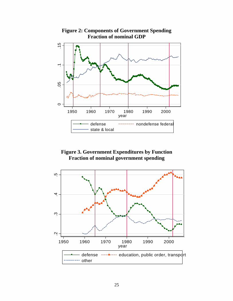
Figure 2: Components of Government Spending Fraction of nominal GDP

0.0

5.1

.15

1950 1960 1970 1980 1990 2000year

defense nondefense federalstate & local

Figure 3. Government Expenditures by Function Fraction of nominal government spending

.2.3

.4.5

1950 1960 1970 1980 1990 2000year

defense education, public order, transportother

25

Figure 4A. Comparison of Identification Methods Response to a government spending shock

(Standard error bands are 68% confidence intervals)

VAR Shocks War Dates

0.4

.81.

2

0 4 8 12 16 20quarter

government spending

0.4

.81.

20 4 8 12 16 20

quarter

government spending

-.10

.1.2

.3.4

0 4 8 12 16 20quarter

gdp

-.10

.1.2

.3.4

0 4 8 12 16 20quarter

gdp

-.12

0.1

2.2

5

0 4 8 12 16 20quarter

total hours

-.12

0.1

2.2

5

0 4 8 12 16 20quarter

total hours

26

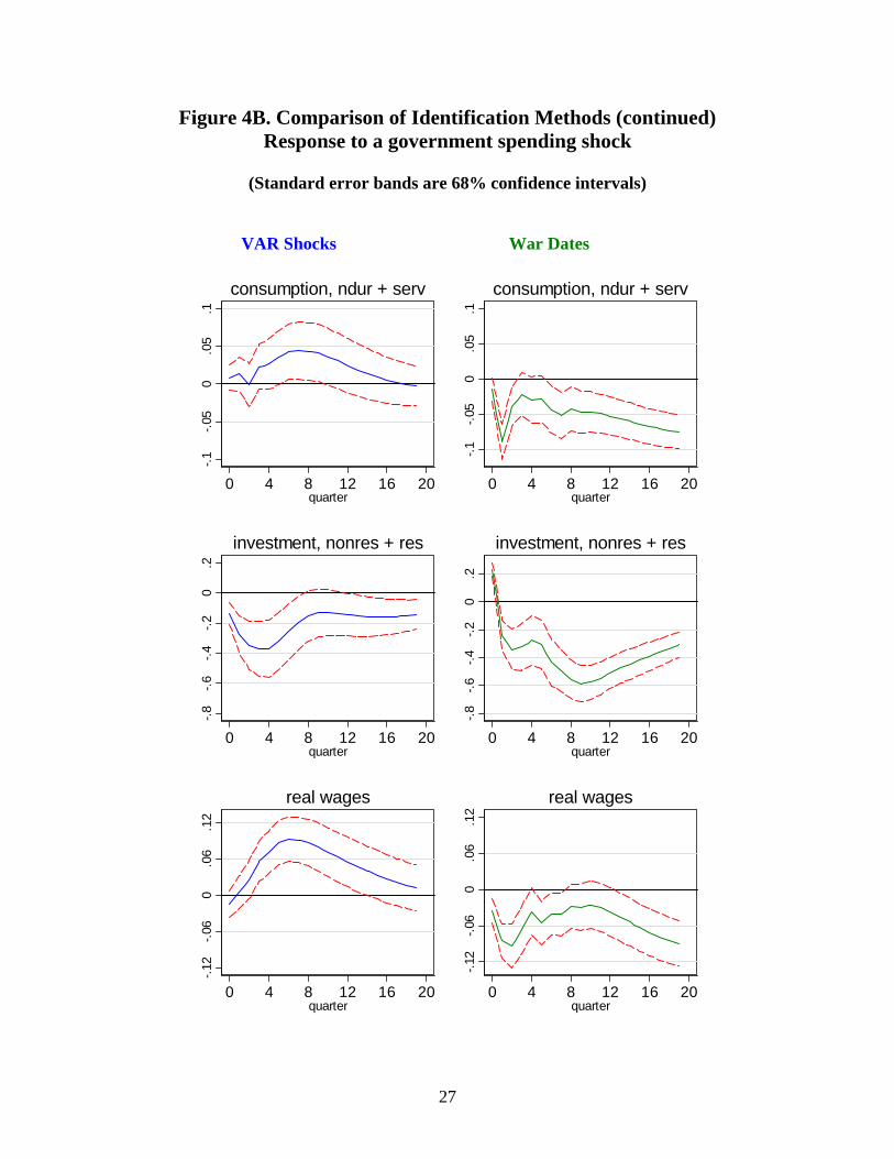
Figure 4B. Comparison of Identification Methods (continued) Response to a government spending shock

(Standard error bands are 68% confidence intervals)

VAR Shocks War Dates

-.1-.0

50

.05

.1

0 4 8 12 16 20quarter

consumption, ndur + serv

-.1-.0

50

.05

.10 4 8 12 16 20

quarter

consumption, ndur + serv

-.8-.6

-.4-.2

0.2

0 4 8 12 16 20quarter

investment, nonres + res

-.8-.6

-.4-.2

0.2

0 4 8 12 16 20quarter

investment, nonres + res

-.12

-.06

0.0

6.1

2

0 4 8 12 16 20quarter

real wages

-.12

-.06

0.0

6.1

2

0 4 8 12 16 20quarter

real wages

27

Figure 5: Episodes of Defense Spending and VAR Defense Shocks 0

.2.4

.6.8

1

1948 1949 1950 1951 1952 1953 1954 1955

Defense Spending During Korean War

.5.6

.7.8

1964 1965 1966 1967 1968 1969 1970

Defense Spending During Vietnam War

-.05

0.0

5.1

.15

1948 1949 1950 1951 1952 1953 1954 1955

VAR Shocks During Korean War

-.04

-.02

0.0

2.0

4

1964 1965 1966 1967 1968 1969 1970

VAR Shocks During Vietnam War

.2.3

.4.5

.6

1978 1980 1982 1984 1986

Defense Spending During Carter-Reagan Build-Up

.25

.3.3

5.4

.45

1999 2000 2001 2002 2003 2004

Defense Spending During 9/11

-.02

0.0

2.0

4

1978 1980 1982 1984 1986

VAR Shocks During Carter-Reagan Build-Up

-.1-.0

50

.05

.1

1999 2000 2001 2002 2003 2004

VAR Shocks During 9/11

28

Figure 6. The Effect of an Increase in Government Spending Announced Two Quarters in Advance

0.0

2.0

4.0

6gg

0 4 8 12 16 20quarter

government spending

0.0

5.1

.15

.2.2

5yg

0 4 8 12 16 20quarter

gdp0

.04

.08

.12

ng

0 4 8 12 16 20quarter

hours-.2

-.10

cg

0 4 8 12 16 20quarter

consumption

-.20

.2.4

ig

0 4 8 12 16 20quarter

investment

-.002

-.001

0w

g

0 4 8 12 16 20quarter

real wages

29

Figure 7A. The Effect of Missing the Timing

Based on VARs on model simulations in which government spending changes are anticipated two quarter in advance

Faulty Timing True Timing

0.4

.81.

2

0 4 8 12 16 20quarter

government spending

0.4

.81.

2

0 4 8 12 16 20quarter

government spending

-.005

0.0

05.0

1.0

15

0 4 8 12 16 20quarter

gdp

-.005

0.0

05.0

1.0

15

0 4 8 12 16 20quarter

gdp

-.001

0.0

02.0

04.0

06

0 4 8 12 16 20quarter

hours

-.001

0.0

02.0

04.0

06

0 4 8 12 16 20quarter

hours

30

Figure 7B. The Effect of Missing the Timing

Based on VARs on model simulations in which government spending changes are anticipated two quarter in advance

Faulty Timing True Timing

-.006

-.002

0.0

02.0

04

0 4 8 12 16 20quarter

consumption

-.006

-.002

0.0

02.0

04

0 4 8 12 16 20quarter

consumption

-.03

-.01

0.0

1.0

3

0 4 8 12 16 20quarter

investment

-.03

-.01

0.0

1.0

3

0 4 8 12 16 20quarter

investment

-.001

5-.0

005

0.0

005

.001

5

0 4 8 12 16 20quarter

real wages

-.001

5-.0

005

0.0

005

.001

5

0 4 8 12 16 20quarter

real wages

31

Figure 8. The Effect of Mistiming the Ramey-Shapiro Dates (The Ramey-Shapiro dates are shifted later to coincide with

the large positive VAR shocks in 1951:1, 1965:3 1980:4 2003:2)

-.20

.2.4

.6

0 4 8 12 16 20quarter

government spending

-.10

.1.2

.3

0 4 8 12 16 20quarter

gdp

-.10

.1.2

0 4 8 12 16 20quarter

total hours

-.05

0.0

5.1

0 4 8 12 16 20quarter

consumption, ndur + serv

-.20

.2.4

0 4 8 12 16 20quarter

investment, nonres + res

-.05

0.0

5.1

0 4 8 12 16 20quarter

real wages

32

Figure 9: The Impact of Defense Shocks Using the New Narrative-Based Defense Shocks

0.4

.81.

2

0 4 8 12 16 20quarter

government spending

-.10

.1.2

.3.4

0 4 8 12 16 20quarter

gdp-.1

20

.12

.25

0 4 8 12 16 20quarter

total hours-.1

-.05

0.0

5.1

0 4 8 12 16 20quarter

consumption, ndur + serv

-.8-.6

-.4-.2

0.2

0 4 8 12 16 20quarter

investment, nonres + res

-.12

-.06

0.0

6.1

2

0 4 8 12 16 20quarter

real wages

33