Embed Size (px)
Citation preview

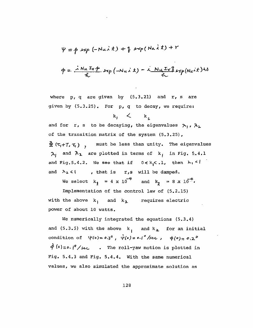
R-930
SATELLITE ATTITUDE PREDICTION BY
MULTIPLE TIME SCALES METHOD
by Yee-Choe Tao
and Rudrapatna Ramnath
December 1975
N76-21252(1AS-C4-4L742) SATILLITE ATTITUDE PREDICTION BY MULTIPLE TIME SCALES METHOD
(Charles Stark)Lab Inc) 205 pI(Draper lnclasCSCL 220
FHO 5 G317 24612 j
The Charles Stark Draper Laboratory Inc Cambridge Massachusetts 02139
R-930
SATELLITE ATTITUDE PREDICTION BY
MULTIPLE TIME SCALES METHOD
by
Yee-Chee Tao Rudrapatna Ramnath
December 1975
Approved P4A 13AJ i
Norman E Sears A $t
The Charles Stark Draper Laboratory Inc Cambridge Massachusetts 02139
ACKNOWLEDGMENT
This report was prepared by The Charles Stark Draper
Laboratory Inc under Contract NAS 5-20848 with the Goddard
Space Flight Center of the National Aeronautics and Space
Administration
Publication of this report does not constitute approval
by NASA of the findings or conclusions contained herein
It is published for the exchange and stimulation of ideas
2
ABSTRACT
An investigation is made of the problem of predicting
the attitude of satellites under the influence of external
disturbing torques The attitude dynamics are first
expressed in a perturbation formulation which is then
solved by the multiple scales approach The independent
variable time is extended into new scales fast slow
etc and the integration is carried out separately in
the new variables The rapid and slow aspects of the
dynamics are thus systematically separated resulting
in a more rapid computer implementation The theory is
applied to two different satellite configurations rigid
body and dual spin each of which may have an asymmetric
mass distribution The disturbing torques considered
are gravity gradient and geomagnetic A comparison
with conventional numerical integration shows that our
approach is faster by an order of magnitude
Finally as multiple time scales approach separates
slow and fast behaviors of satellite attitude motion
this property is used for the design of an attitude
control device A nutation damping control loop using
the geomagnetic torque for an earth pointing dual spin
satellite is designed in terms of the slow equation
3
TABLE OF CONTENTS
Chapter Page
1 INTRODUCTION 8
11 General Background 8
12 Problem Description 10
13 Historical Review and Literature Survey 13
14 Arrangement of the Dissertation 16
2 REVIEW OF MULTIPLE TIME SCALES (MTS) METHOD 18
21 Introduction 18
22 MTS and Secular Type of Problems 19
23 MTS Method and Singular Perturbation Problems 27
3 PREDICTION OF ATTITUDE MOTION FOR A RIGID BODY SATELLITE 31
31 Introduction 31
32 Rigid Body Rotational Dynamics 32
33 Euler-Poinsot Problem 37
34 Disturbing Torques on a Satellite 52
35 Asymptotic Approach for Attitude Motion with Small Disturbances 62
36 Attitude Motion with Gravity Gradient Torque 79
37 Satellite Attitude Motion with Geomagnetic Torque 87
4
TABLE OF CONTENTS (Cont)
Chapter Page
4 PREDICTION OF ATTITUDE MOTION FOR A DUAL
SPIN SATELLITE 89
41 Introduction 89
42 Rotational Dynamics of a Dual Spin Satellite 91
43 The Torque Free Solution 92
44 The Asymptotic Solution and Numerical Results 99
5 DESIGN OF A MAGNETIC ATTITUDE CONTROL SYSTEM
USING MTS METHOD 103
51 Introduction 103
52 Problem Formulation 104
53 System Analysis 113
54 An Example 127
55 Another Approach By Generalized Multiple Scales (GMS) Method Using Nonlinear Clocks29
6 CONCLUSIONS AND SUGGESTIONS FOR FUTURE RESEARCH 131
61 Conclusions 131
62 Suggestions for Future Research 133
Appendix -1-135
A AN EXPRESSION FOR (Im Q 1
BEXPANSION OF 6-l N 137 -I-
1E S
LIST OF REFERENCES 139
5
LIST OF ILLUSTRATIONS
Figure Page
341 Torques on a satellite of the earth as a
function of orbit height 52
361
i 3612
Simulation errors in rigid body case (Gravity gradient torque)
145
3613 Maximim simulation errors 157
3614 Computer time 157
371 Simulation errors in rigid body case 158 +(Geomagnetic torque)
3712
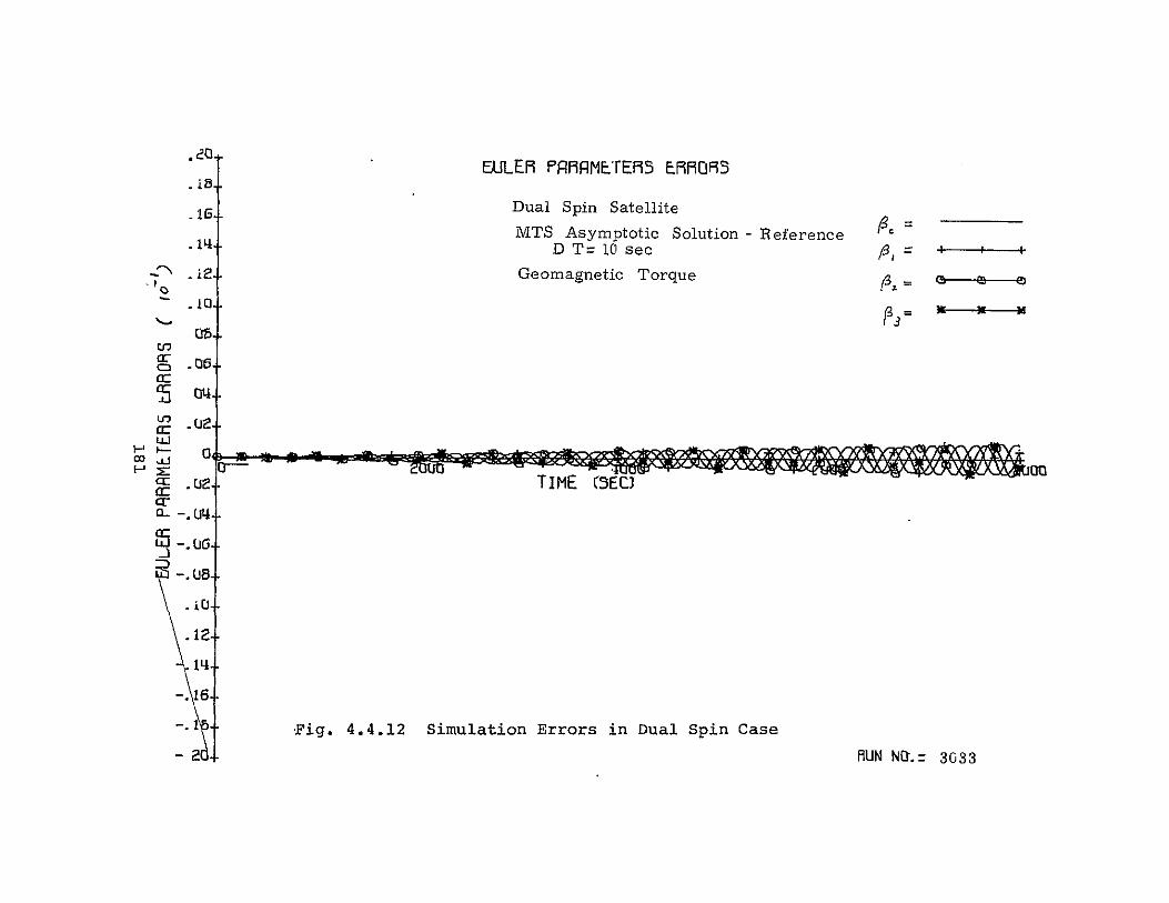
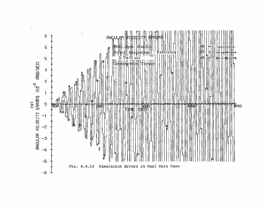
441 Simulation errors in dual spin case 170
4418 (Gravity gradient and geomagnetic torques)
51 Roll yaw and pitch axes 105
541 Eigenvalue 0 1881
542 Eigenvalue 2 188
543 Roll and yaw motions 189+ 558
6
LIST OF TABLES
Table Page
361 Rigid body satellite disturbed by gravity gradient torque 201
371 Rigid body satellite disturbed by geomagnetic torque202
441 Dual spin satellite disturbed by gravity gradient torque 203
442 Dual spin satellite disturbed by geomagnetic torque 204
55 GMS Approximation and direct integration 205
7
CHAPTER 1
INTRODUCTION
11 General Background
The problem of predicting a satellite attitude motion
under the influence of its environmental torques is of
fundamental importance to many problems in space research
An example is the determination of required control torque
as well as the amount of fuel or energy for the satellite
attitude control devices Similarly a better prediction
of the satellite attitude motion can be helpful in yielding
more accurate data for many onboard experiments such as
the measurement of the geomagnetic field or the upper
atmosphere density etc which depend on the satellite
orientation
Yet the problem of satellite attitude prediction
is still one of the more difficult problems confronting
space engineers today Mathematically the problem conshy
sists of integrating a set of non-linear differential
equations with given initial conditionssuch that the
satellite attitude motion can be found as functions of
time However the process of integrating these
equations by a direct numerical method for long time intershy
vals such as hours days (which could be even months or
OP DGI0 QPAGE L9
years) is practically prohibited for reasons of compushy
tational cost and possible propagation of numerical
round-off and truncation errors On the other hand it
is even more difficult if it is possible at all to
have an exact analytic solution of the problem because
of the non-linearity and the existence of various external
disturbing torques in each circumstance
A reasonable alternative approach to the above problem
seems to be to apply an asymptotic technique for yielding an
approximate solution The purpose of this approach is
to reduce the computational effort in the task of attitude
prediction for long intervals at the cost of introducing
some asymptotic approximation errors Meanwhile the
asymptotic approximate solution has to be numerically
implemented in order to make it capable of handling a
broad class of situations
We found the problem is interesting and challenging
in two ways Firstbecause it is basic the results
may have many applications Second the problem is very
complicated even an approximate approach is difficult
both from analytic and numerical points of view
ORTGRTAI-PAGr OF POOR QUAULI4
9
12 Problem Description
The subject of this thesis is the prediction of
satellite attitude motion under the influence of various
disturbing torques The main objective is to formulate
a fast and accurate way of simulating the attitude rotashy
tional dynamics in terms of the angular velocity and
Euler parameters as functions of time The formulation
has to be general it must be able to handle any orbit
initial conditions or satellite mass distribution Furshy
thermore it must predict the long term secular effects
and or the complete attitude rotational motion depending
on the requirement Because of this built-in generality
it is intended that the program can be used as a design
tool for many practical space engineering designs To
achieve this desired end the problem is first expressed
as an Encke formulation Then the multiple time scales
(MTS) technique is applied to obtain a uniformly valid
asymptotic approximate solution to first order for the
perturbed attitude dynamics
Two different satellite configurations are considered
a rigid body satellite and a dual spin satellite each of
which may have an asymmetric mass distribution In the
latter case it is assumed that the satellite contains a
single fly wheel mounted along one of the satellite
10
body-principal-axes to stabilize the satellite attitude
motion These models are considered typical of many
classes of satellites in operation today The disturbing
torques considered in this dissertation are the gravity
gradient and the geomagnetic torques For a high-orbit
earth satellite these two torques are at least a hundred
times bigger than any other possible disturbance though
of course there would be no difficulty inserting models
of other perturbations
Both the gravity gradient and the geomagnetic torques
depend on the position as well as the attitude of the sateshy
llite with respect to the earth Therefore the orbital
and attitude motion are slowly mixed by the actions of
these disturbances However the attitude motion of the
vehicle about its center of mass could occur at a much
faster rate than the motion of the vehicle in orbit around
the earth Directly integrating this mixed motion fast
and slow together is very inefficient in terms of comshy
puter time However realizing that there are these
different rates then the ratio of the averaged orbital
angular velocity to the averaged attitude angular veloshy
city or equivalently the ratio of the orbital and attitude
frequencies (a small parameter denoted S ) may be used in
the MTS technique to separate the slow orbital motion
from the fast attitude motion In this way the original
11
PAGE IS OP PoO QUau
dynamics are replaced by two differential equations in
terms of a slow and a fast time scale respectively
The secular effect as well as the orbit-attitude coupling is
then given by the equation in the slow time scalewhile
the non-biased oscillatory motion is given by the second
equation in terms of the fast time scale In addition
a method for handling the resonance problem is also discussed
In some situations the slow equation for the secular
effects can be useful in the design of an attitude control
system The vehicle environment torques if properly
used can be harnessed as a control force However- to
design such a control system it is often found that the
control force is much too small to analyze the problem
in the usual way In fact the design is facilitated in
terms of the equation of the slow variable because only
the long term secular motions can be affected This
application is demonstrated by mean of a nutation damping
control loop using the geomagnetic torque
ORICGIktPk~OF POOR
12
13 Historical Review and Literature Survey
The problem of attitude dynamics of an artificial
-satellite rigid body as well as dual spin case is
closely related to the branch of mechanics of rigid body
rotational motion The subject is regarded as one of
the oldest branches of science starting from middle of
the eighteenth century Since then it has interested
many brilliant minds for generations The literature
in this area therefore is rich and vast Thus we have
to focus our attention on only those areas which are
immediately related to this research
The classical approach to the rotational dynamics
mainly seeks the analytic solutions and their geometric
interpretations By this approach many important and
elegant results have been obtained Among them the
Poinsot construction of L Poinsot (11] gives a geoshy
metrical representation of the rigid body rotational
motion The Euler-Poinsot problemfor a torque-free
motion was first solved by G Kirchhoff[12] by means of
Jacobian elliptic functions On the other hand F
Klein and A Sommerfeld [13] formulated the same problem
in terms of the singularity-free Euler symmetric parashy
meters and gave the solution Recently H Morton J
Junkins and others [15] solved the equations of Euler
symmetric parameters again by introducing a set of complex
orientation parameters Kirchhoffs solution as well as
13
the solution of Euler symmetric parameters by H Morton etcshy
play an important role- as a reference trajectory- in our
study
This approachhowever because of its nature can
not handle a general problem for various situations This
difficulty is substantial for the case of an artificial
satellite A more flexible alternativewidely applied in
the engineering world is the asymptotic technique for
evaluating an approximate solution Among them the
averaging method by N N Bogoliubov and Y Mitropolsky
[14] is the most commonly used For example Holland and
Sperling[16] have used the averaging method for estimating
the slow variational motion of the satellite angular
momentum vector under the influence of gravity gradient
torque and Beletskii [17] formulated perturbation
equations using the osculating elements for a dynamically
symmetric satellite F L Chernousko [18] derived
the equations of variation of parameters for angular
momentum vector and the rotational kinetic energy for
an asymmetric satellite However the averaging method
is most easily appied for a problem which normally has
a set of constant parameters such that the slow variational
behavior of these parameters can be established in a
perturbed situation For example in a simple harmonic
oscillator the frequency and amplitude are two parashy
meters which characterize the dynamics described by a
14
second order differential equation Unfortunately
rotational motion in generaldoes not immediately lead
to a complete set of similar parameters Although it
has constant angular momentum vector and kinetic energy
as parameters it is a six-dimensional problem Besides
an elliptic integral is involed in its solution Nevershy
theless this difficulty can be overcome by casting the
problem in a Hamilton-Jacobi formfrom which a variationshy
of-parameter formulation can be derived in terms of
Jacobi elements This approach is reflected in the works
of Hitzl and Breakwell [19] Cochran[20] Pringle[21] etc
Our dissertation is different from the others
mainly in three aspects First it is a new approach
using the multiple time-scales method [1-7] with the
Encke perturbation formulation [22] for predicting the
complete satellite attitude motion without involving the
Hamilton-Jacobi equation Second we are interested in
the secular effect of the disturbing torques as well
as the non-secular oscillatory effect By combining
them we have the complete solution Further we know
that the former gives the long term behavior and the
latter indicates the high-frequency motion of the sateshy
llite attitude dynamics Third our immediate objective
is numerically oriented for saving computer time Thus
the difficulties we encounter could be analytical as
well as numerical
15
14 Arrangement of the Dissertation
Chapter 2 reviews the multiple time scales asymptotic
technique - a basic tool in this research Two examples
are used for illustrating the fundamental procedureone
represents the secular type of almost-linear problem
and the other represents the singular type of slowly
time-varying linear system
Chapter 3 develops the asymptotic solution to the
attitude motion of a rigid body satellite under the influshy
ence of known small external torques It shows that
the original equations of attitude dynamics can be represhy
sented by two separate equations - one describing the
slow secular effects and the other describing the fast
oscillatory motion The latter can be analytically
evaluated Numerical simulation using this approach is
also presented for the class of rigid body satellites
under the influence of gravity gradient and geomagnetic
torques
In chapter 4 the previous results are extended
to the case of dual spin satellite in which a fly-wheel
is mounted onboard Two sets of numerical simulations
one for a dual-spin satellite in the earth gravity
gradient field and the other influenced by the geomagnetic
field are given
16
Chapter 5 represents an application of the fact that
MTS method separates the slow and fast behaviors of a satelshy
lite attitude motion We demonstrate that the slow equation
which describes the secular effects can be useful in the
design of a satellite attitude control system A
nutation damping feedback control loopusing the geomagshy
netic torque for an earth pointing dual-spin satellite
is designed in terms of the slow equation
In chapter 6 the conclusions drawn from the results
of this study are summarized and some suggestions for
future research are listed
17
CHAPTER 2
REVIEW OF MULTIPLE TIME SCALES (MTS) METHOD
21 Introduction
multiple time scales (MTS) method is one of the
relatively newly developed asymptotic techniques It
enables us to develop approximate solutions to some
complicated problems involving a small parameter S I
when the exact solutions are difficult if not impossible
to find The basic concept of MTS method is to extend
the independent variable usually time into multi-dimenshy
sions They are then used together with the expansion of
the solution (dependent variable) such that an extra degree
of freedom is created and the artificial secular terms can
be removed Thus a uniformly valid approximate solution
is obtained [1-7]
An unique feature of the MTS method is that it can
handle secular type as well as singular type of perturbation
problems in a unified approach By this method the fast
and slow behaviors of the dynamics are systematically idenshy
tified and separated The rapid motion is given in terms
of a fast time scale and the slow motion in terms of a
slow time scale each of which in most cases has a
meaningful physical explanation A comprehensive refershy
ence on this subject is by Ramnath[3] The textbook by
Nayfeh [7] has also been found informative
18
22 MTS and Secular Type of Problems
A secular perturbation problem is one in which
the nonuniformity in a direct expansion occurs for large
values of the independent variable We consider systems
with a small forcing term The forcing term changes
the dynamics gradually and has no appreciable effect in
a short time However the long time secular effect of
the small forcing term may significantly influence the
overall behavior of the dynamics From a mathematical
point of view a secular type of problem has a singularity
at infinty in the time domain
Since perturbation problems and the asymptotic
technique for solving them can be most easily understood
by solving a demonstration case let us consider a simple
example of a slowly damped linear oscillator [7]
X + X =- x 0 (221)
where E is a small parameter The simplicity of the
forcing term -ZE allows us to interpret the approximate
solution developed later The exact solution is available
but the generality of our asymptotic approach will not be
lost in spite of the simple form of the forcing term
We first solve the problem by Poincare type of
direct expansion method [33] such that difficulties of
non-uniformity and secular terms can be illustrated
Then the same problem is solved by MTS method which
19
QUAL4T
yields a uniformly valid asymptotic solution to first
order
We expand X() into an asymptotic series in E
X() -- + S i + Sz+
S ) it)()(222)
An asymptotic series is defined [9] as one in which
the magnitude of each term is at least one order less than
its previous one lie ISni IsI = Xn -IXt- I A ItIxi
Therefore S) decreases rapidly as the index i increases
This simple fact allows us to approximate the solution by
calculating only a few leading terms in the series expansion
Substituting(212) into (211) and equating the
coefficients of like powers of E we have
a
o (223)
(224)
20
The solution for () in equation (223) is
)1--- CA- 4 I (225)
Where a and b are two constants Substituting
Yo into eq (224) of x
+I + y-| -2 6 (226)
kifh IC
The solution is Z
aeI0 =CC bt (227)
The approximation of x(t) up to first order is
therefore
= (O Oa+bA4j (- 4 tat-122-At4 --Akt)
(228)
Above approximation however is a poor one because
of the occurrence of two terms - ASf CaA and - 6 F
which approach infinity as X-O They are referred
to as secular terms We know the true x(t) has to be
bounded and asymptotically decaying for x(t) is a
damped harmonic oscillator The secular terms
21
make the series expansion Xt)=z4-1-E1+ in
eq (228) a non-asymptotic one since _ _ = F__3 X6
as -o In the process of finding a solution by series
expansion there is no guarantee that the higher order terms
can be ignored in a non-asymptotic series expansion On the
other hand if an asymptotic series is truncated the error
due to the ignored higher order terms will be uniformly
bounded in a sense that lerrorl (approximate solution
SE An approximate solution is said to be uniformly
valid if its error is uniformly bounded in the interval of
interest We see -that the loss of accuracy
by straightforward Poincare type of expansion is due to the
occurrence of the secular terms and therefore the approxishy
mation is not uniformly valid
In the following the same problem will be studied in
the context of multiple time scale method which yields a
uniformly valid solution
For convenience we rewrite the dynamics
X +- ZX (229)
The solution (U) is first expanded into an asymptotic
series of pound same as before
X(-k) Xot)+ (2210)
The concept of extension is then invoked which
22
O0
expands the domain of the independent variable into a space
of many independent variables These new independent
variables as well as the new terms that arise due to
extension are then so chosen that the non-uniformities
of direct perturbation can be eliminated [3]
Let
t- CL-r rI 1 3 (2211)
For an almost linear problem as the one we are studying
rtt
The new time scales in general can be non-linear
as well as complex which depend upon the nature of the
problem [4] However for this particular problem a set of
simple linear time scales works just as well
The time derivative can be extended in the
space by partial derivatives as follows
oA o=d+a OLt
-C at1 OLd _
23
And
__- 7 I
Substituting equations (2212) (2213) and (2210)
into equation (229) and equating coefficients of like
powers of E we have
4 shy (2214)
(2215)
The original equation has been replaced by a set of
partial differential equations The solution for -(A)
from (2214) is
(2216)
where ab are functions of ti-q etc and are
yet to be determined Substitute Y- from (2216) into
(2215) and solve for x
-F
4 -k-irp(-Ax 0 ) (Zb1i -amp)
(2217)
24
Equation (2217) represents a harmonic oscillator
driven by an external sinusoidal function The
Xl( ) could become unlimited since the external force
has the same natural frequency as the system itself
In order to have 1X1X0 l bounded the terms to the right
hand side of the equal sign in (2217) have to be
set to zero which will result in a bounded X1 () Note
that this is possible because there is a freedom of
selecting functions a and b from the extension of the
independent variable By doing so we have
(2218)i Zb +2 ___Zcf
or
(2219)
where 6L0 and are two constants Combining
(2216) and (2219)the approximate solution for X(t)
up to first order of E by MTS method is
Y=0 +o Ep - 0I4b op
(2220)
25
The exact solution for (229) can be obtained
which is
4- bKt~l(-XYWW iit)7 (2221)
The errorsolution ratio in this case is
xa 0error I Xe~t Xaproi O(et) IX
It is interesting to note that by the MTS method
we have replaced the original dynamics (229) by an
equation (2214) in the fast time scale T
+ + n XC = 0 (2214)
and two slow equations in the slow time scale Z
tIT 6b 6 0 (2218)
The fast equation gives the undisturbed oscillatory
motion and the slow equations represent the slow variashy
tional change of the amplitude of the oscillation caused
26
by the damping term
23 MTS M4ethod and Singular Perturbation Problems
There is a class of perturbation problems in which
the behavior of the reduced system - by setting 6
equal to zero - could be dramatically different from the
original This phenomenon occurs because the reduced
system described by a lower order differential equation
can not satisfy the given boundary conditions in general
We call this kind of problem a singular perturbation
problem
Singular perturbation problems have played an
important role in the engineering field most notably
in fluid mechanics for eg the boundary layer theory
This problem was solved by introducing the inner (Prandtls
boundary layer) and outer expansion [32] However
the same problem also can be solved in a more straightshy
forward approach by the MTS method This approach was
first noted in the paper by Ramnath [4] in studying the
behavior of a slowly time-variant linear system by
employing non-linear time scales In the following let
us use an example which is adopted from [3] for demonshy
stration
27
AaG1oo1GINA
of -POORQUIJ~
Consider a second order singular perturbation problem
2y + W (t)Y(231)
Where Olt FCltltI -is a constant small parameter
Expand the time domain t into two-dimensions
and define Z0 Z2 as -follows
(232)
at
where 4(t) is yet to be determined
The time derivative - and can be extended as
Sc - azAe (233)
At2 +2 t4 (Zr)
44
Substituting (233) into (231) and separating terms
according to the pover of F we will have the set of
equations
28
4 fl + W L) zo (234)
6
+
y -- (236)
Y I-V(235)
=0
By assuming that has a solution in the form
=) oLz) Px(zI ) (237)
substitution into (234) yields
+t- W(-Cc) shy
(238)
Similarly put (237) into (235) we have
4- Zlt + k(239)
o - (2310)
The approximate solution up to first order can be
constructed as
29
-I -I
f k j 2C Aitptf ftJ tir(tw
(2311)
We obtain (2311) from (238) and (2310)
Note that in our approximation the frequency variation
is described on the tI scale and the amplitude variation
on the XC scale The success of this approach depends
on the proper choice of the nonlinear clock While in
the past this choice was made on intuitive grounds
recent work [2 ] has been directed towards a systematic
determation of the clocks Ramnath [3 ] has shown that
the best nonlinear clocks can be determined purely in
a deductive manner from the governing equations of the
system With a judicious choice of scales the accuracy
of the asymptotic approximation is assured A detailed
error analysis of the approximation was given by Ramnath
[3 ] These questions are beyond the scope of the
present effort and reference [3 1 may be consulted for
more information
30
CHAPTER 3
PREDICTION OF ATTITUDE MOTION FOR A RIGID BODY SATELLITE
31 Introduction
In this chapter a multiple time scales asymptotic
technique is applied for the prediction of a rigid body
satellite attitude motion disturbed by a small external
torque
The attitude dynamics of a satellite described in
terms of the Eulers equations and Euler symmetric parashy
meters are first perturbed into an Encke formulation
in which the torque-free case is considered as a nominal
solution The multiple time scales technique is then
used for the separation of the fast attitude motion from
the slow orbital motion in an approximate but asymptotic
way Thereby the original dynamics can be replaced by
two sets of partial differential equations in terms of a
slow and a fast time scale The long-term secular effects
due to the disturbing torque are given by the equations
in the slow time scale which operate at the same rate as
the orbital motion A non-biased oscillatory motion is
given by the second set of equations in terms of the fast
time scale which basically describes the vehicle attitude
oscillatory mQtion These fast and slow motions combined
31
give us a first order asymptotic solution to the Enckes
perturbational equation which)therefore~can be regarded
as the second order asymptotic solution to the original
satellite attitude dynamics
Finally the fast non-biased oscillatory motion
can be analytically evaluated if the external torques
are not explicitly functions of time Thus numerical
simulation of a satellite rotational motion by this
new approach requires only the integration of the slow
equation which can be done with a large integration
time step This fact leads to a significant saving of
computer time as compared to a direct numerical inteshy
gration Two examples one with gravity gradient torque
the other with geomagnetic torque are demonstrated in
section 36 and 37
32 Rigid Body Rotational Dynamics
(A) Eulers Equations
Newtons second law for rigid body rotational motion
in an inertial frame can be written as
A (321)
Where H and M are the angular momentum and the
external torque By Coriolis law the motion can be
32
expressed in any moving frame b as
o (322)
Where V is the angular velocity of the b
frame with respect to the inertial frame In case the
b frame is selected to coincide with the body fixed
principal axes (xyz) then the angular momentum can be
written as
q6= Ix 0 o WX TX Vj (
my 0 lo T W(
(3deg23)
where xI ly I IS are moments of inertia about x y z axes
Combining (322) and (323) we have Eulers equations
Y t 9 ( 3 1M (324)
In vector notation they are
33
I 4Ux I(FV M (325)
Eulers equations give the angular velocity of a
rigid body with respect to an inertial space though this
angular velocity is expressed in the instantaneous body
fixed principal axes [35]
(B) Euler Symmetric Parameters
The role of Euler symmetric parameters are
similar to Euler angles which define the relative
orientation between two coordinates From either of
them a transformation matrix can be calculated and a
vector can be transformed from one coordinate to another
by pre-multiplying with the transformation matrix
However from an application point of view there are
notable differences between Euler symmetric parameters
and Euler angles The important ones are listed as follows
1 Euler angles ( = I3 23) have order of three
whereas Euler symmetric parameters ( 2= 123)
have order of four with one constraint
2 pi are free from singularitywhere Gez are
not Since 19 ) 2 0 are the z-x-z rotations
in case that =o one can not distinguishG
34
from 03
3 1fl propagate by a linear homogenous differential
equation 9 are by a non-linear differential
equation
4 Oz have a clear physical interpretation -ie
precession nutation and rotation 9 can not
be immediately visualized
By considering above differences we feel that
Euler symmetric parameters are more suitable for numerical
computation because they are propagated by a linear
equation and free from singularity even though they add
one more dimension to the problem On the other hand
Euler angles are easier to understand In this chapter
we select Euler symmetric parameters for the satellite
attitude prediction problem And in chapter 5 for a
satellite attitude control system design we use Euler
angles
The concept of Euler symmetric parameters is based
upon Euler Theorem which says that a completely general
angular displacement of a rigid body can be accomplished
by a single rotation 4) about a unit vector (j A
where 2 is fixed to both body and reference frames
The are then defined as
35
A L4i 3 ( 3 2 6 )PZ
with a constraint 3
J(327)= =
If CYb is the transformation matrix from the
reference frame r to the frame b
=Vb cv 6 VY
Then Crb can be calculated in term of as [35]
2 (A 3)C~~--- -f-3-102(p1 3 - - - jptt) a(4l-tJ
=~21Pp ~ 2 A3 2 z (l AA
(328)
Also Pi satisfy a homogeneous linear differential
equation [35]
0 WX WJ V 3
__ X (329)
-W Po
36
-b
where tx is the component of WAi in x direction etc
33 Euler-Poinsot Problem
Closed form solutions for a rigid body rotational
motion with external torque are usually not possible
except for a few special cases A particular one named
after Euler and Poinsot is the zero external torque
case This is useful here since the disturbing
torques acting on a satellite are small the Euler-Poinsot
case can be taken as a nominal trajectory
It is Kirchhoff [12] who first derived the complete
analytic solution for Eulers equation (amp1) in terms of
time in which an elliptic integral of the first kind is
involved In the following we will review the Kirchhoffs
solution along with the solution of Euler symmetric
parameters ( g ) by Morton and Junkins [15] Also
by defining a polhode frequency we find that the solution
foramp can be further simplified such that it contains
only periodic functions
(A) Kirchhoffs Solution
Without external torque Eulers equations are
Wx 3 W L) 0
J JA (3321)
37
tJL~xx) ~ 03 (333)
Above equations are equivalent to a third order
homogeneous ordinary differential equation and its solushy
tion involves three integration constants
Multiplying above three equations by Wx Wy and W
respectively and integrating the sum we obtain one of
the integration constants for the problem called T which
is the rotational kinetic energy of the system that is
-A jz+ 4- 4=2 (334)
Similarly by multiplying the three Eulers equations by Ix X ty and x respectively and inteshy
grating the sum we have H another integration constant
that is the angular momenbum of the system
x _ + + Ha -- I(335)
Having rotational energy T and angular momentum H
given a new variable + can be defined in terms of time
t by an elliptic integral of the first kind
T-) (336)
38
where A T and k are constants and k is the
modulus of the elliptic integral
Kirchhoffs solution can be written as follows
Wt -X I- 4 A- rq-) (337)
LOY (338)
W 3 - Cod (339)
where constants atbcrkx andtr are defined as follows
(3310a) IX ( X - T
z2 ZIxT--H b
_
-(3310b)
722 (3310c)
2- ( 3 H(3310d)Ix ly r
42 9- poundjJ xT- (3310e)
-Ie H3
x-( 2 )( 331l0 f )a 39 k
39
=fj () ] (3310g)
Signs of abc and should be picked such that
they satisfy the equation
- - -x (3311)
The validity of above solution can be proved by
direct substitution
Kirchhoffs solution is less popular than
Poinsot construction in the engineering world One
reason is that it involves an elliptic integral
the solution becomes rather unfamiliar to the engineering
analyst However for our long term satellite attitude
prediction problem Kirchhoffs solution seems to be a
powerful tool
(B) Solution For Euler Symmetric Parameters
Euler symmetric parameters satisfy a linear differshy
ential equation which relates W i and j [35]
jP _ i o W03 - W~ z (3312)
P3 L40 0
40
The constraint is
A set of complex numbers lt00 can be introduced
as follows
=I -P3 + Pi (3313)
0(3 1 4-A 13i
where
=IT shy
and c satisfy a constraint of
CY0 0q -j Oe o (3314)
In matrix and vector notations (3312) and (3313)
are
L 13 (3315)
= A (3316)
41
where
X
oX
0
ALoJO
(103
- tA)
-W
and
A
a
1
xL
0
A
0
o
-1
0A
or
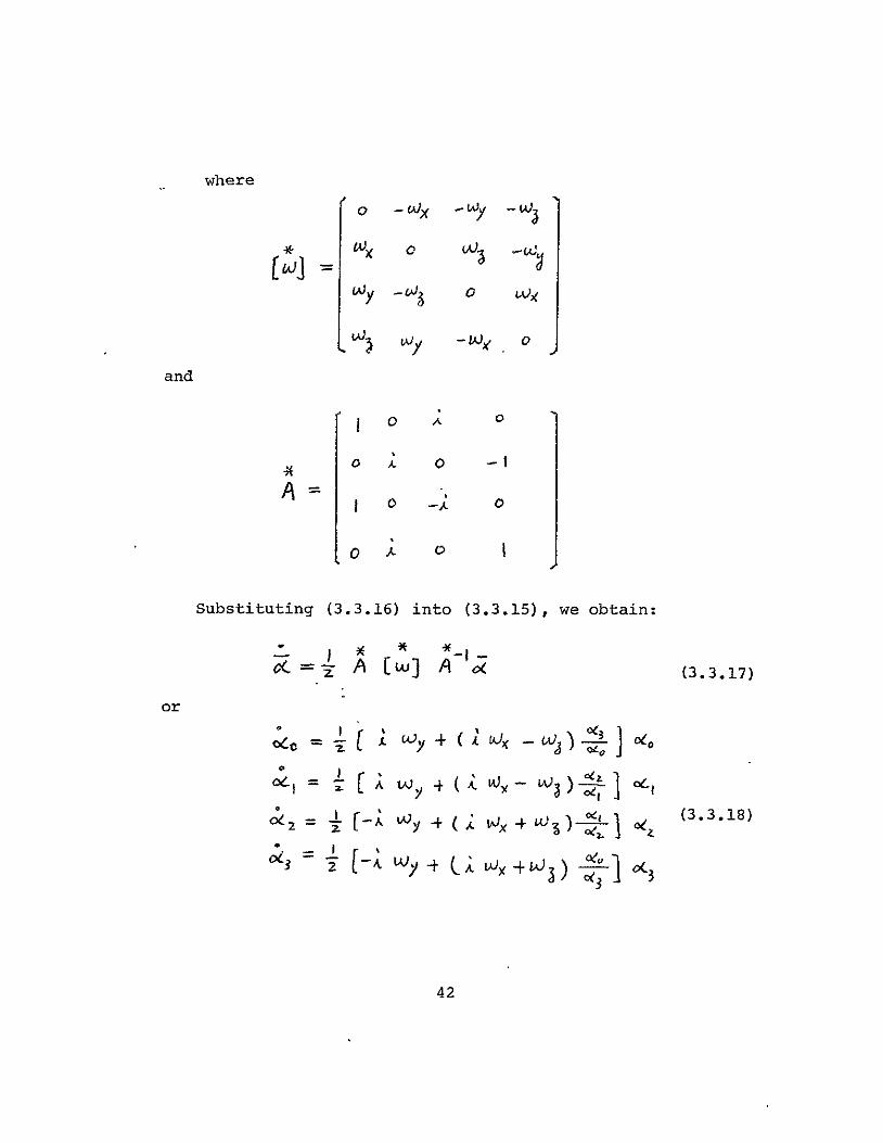
Substituting (3316) into
A Lw] A
(3315)
a
we obtain
(3317)
- i 4
W I2vy
32442x
WY
W
-
)
4 1 104
1C3
ct
0(3
(3318)
42
For a torque - free rigid body rotation the
angular momentum vector H remains constant If we assume
one of our inertial axes (say ) pointing in H direction
and name this particular inertial frame by n then
H j (3319)
Since
6 = C6 H(3320)
combining (3319) (33 20) and (328) we have
-b
H P 4 fi4Pz (3321)
Using the relations
-H an4d
43
(3321) can be written in Wj and oe as
E i-_(4 amp -I o(o ) (3322)
Also o4 satisfy the constraint
0i 0-2 - - 3 = f (3323)
As equations (3322) and (3323) are linear in
0l ampo0 2 G3 and 402 03 they can be solved
in terms of to)( )Waand H ie
amp (z4 L -) (3324)
OCZ_( W -
L 3 74 4 )
DIGNA] PAGE IS OF POO QUAIMTW
The ratio and oL1 can be easily calculated
f-YH( - Wy T3(3325)
-- H T) - -Id k42 3js (3326)
Substituting (3325) and (3326) into equation
(3318) we have
Aoet zA H2w
L01_-t 7- -2T-H (x-tx W)( Ic
ZLy 4u I
Wow we have four decoupled time-variant homogenous
linear equations Their solutions are immediately
45
available in terms of quadratures
Also because (3327) have periodic coefficients
(Wx z theoWc are periodic) by Floquet theory [36]
solution can be expressed in the form Q(t) exp(st) where
Q(t) is a periodic function and s is a constant With
this in mind solutions for (3327) are
o(Ot) E -ao pA ) -wpfr)(Ak
( = U -)siqgtPz) AX ej oto)
(-19) (3328)o4043- Et E A r (-Zgt)A KPI) Pat) d (ko)
where
E = H4 XY LJy(f-)
H+ Jy wy(to)
2
2 -I ) J H - y Vy (to)
H -WH-Pi z -Y
46
XIZT P
and
Ott
2H
11(t) is an elliptic integral of the third kind T
is the period of wx Wy and z and t are reshy
lated by equation (336) Also (t) is given by
6bAA+tf A H
Note there are two frequencies involved in the
solution of Euler symmetric parameters the first one
is the same as the angular velocity W0 WY and Ii
with period of T and the second is related to exp(-rt)
with period of 2 1 The latter one can be explainedR
as due to the motion of the axis of the instantaneous
angular velocity vector WIb In Poinsot
47
construction the tip of the Ui-Jb vector makes a locus on
the invariant plane called the herpolhode 4nd also a
locus on the momentum ellipsoid called polhode The time
required for the vector Ujb to complete a closed
polhode locus is --- We call R the polhode frequency
From =A the general solution for -
is
E) c~zp+ Ejsw(fl4Rf Ez
o0 E (+) Af( pP) 0~ CZP) R) wittnCi+t
(3329)
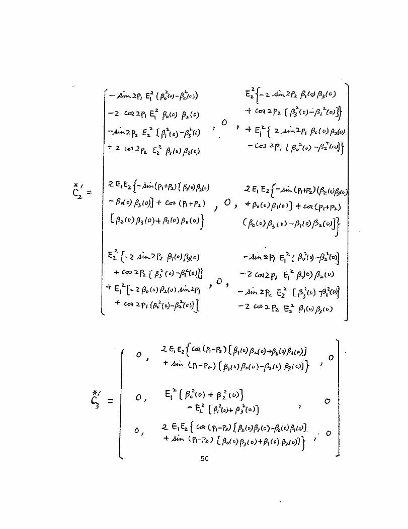
(C) The Transformation Matrix Chb
The transformation matrix C1b in terms of P2
is
t-p 2 + )
48
where Si is given by (3329) By direct substitution we
have
+ Ceb e lztt) (tzt) C+ C3 (3330)
where
Z~ZE 0 3-oAz) + P))
C1 ACut) )IIsz2)3cE)l
+ ( o ZE fz C2Cp+v433 ) Z lI (ItV N
(0)~ ~~ P3 fE 4Y9Pz(OA o Zf 9]amp
2- (o e42P+E
fl-+- -2 ao- E~ N)PfEo)
49
+ C2 2 P1 E ftofg)-Cc 2Pd pc f
E2 A~g0) -2E 2~ amp-
X2 1 pi~tCc )3czo +p p+p) f~jio]+c~~
[l-2At ~~Wso -412-Pj E1[fPJ9-lo
PCc1ript o)Aj o -2 iq2p i(~c o)
c0 ()2~~~~2CQ~ EfampMP)IpE23 P o4 4
C (p-PJ ))PoOt)o Z C-1E j
+ AV~)tpspo~~)13o2
50
Note that matrices C1 C2 and C3 are periodic functions
with period of T only
Summary of the Section
1 Without external torque both Eulers equations and
Euler symmetric parameters can be solved analytically
The solutions are given by equations (337) to
(3310) and (3329)
2 The angular velocity () is a periodic function
that is T(V t+-Twgt (A) whereas P()
contains two different frequencies they are the tshy
frequency and the polhode-frequency
3 The transformation matrix Chb is given by equation
(3330) in which the L -frequency and the
polhode-frequency are factored
ORJOIIVAZ5
51
34 Disturbing Torques on a Satellite
Of all the possible disturbing torques which act
on a satellite the gravity gradient torque (GGT)
and the geomagnetic torque (GMT) are by farthe
most important Fig 341 iliustrates the order of
magnitude of various passive external torques on a typical
satellite [171 in which torques are plotted in terms of
Note that except for very low orbits thealtitude
GGT and the GMT are at least a hundred times as
big as the others
dyne-crn
to
J0
2W 000 000 0 kin
Ia
Figure 341
Torques on a satellite of the Earth as a function of
the orbit heigbt Is afl gravity torque Af aerodyarmic torque
Mf magnetic torqueAr solar radation torque M
micrometeonie impact torque
PAGL ISO0F -poorgUA1X
(A) Gravity Gradient Torque On A Satellite
In this section we first derive the equation for
the GGT second its ordertof magnitude is discussed
third by re-arranging terms we express the GGT equation
in a particular form by grouping the orbit-influenced
terms and the attitude-influenced terms separately so
that it can be handily applied in our asymptotic analysis
1 Equation for Gravity Gradient Torque
with Rf and c as defined in Fig 341
let R = IRI and further define r = R +P and r In
satellite
Xi
C- center of mass
R- position vector
Fig 341
53
- --
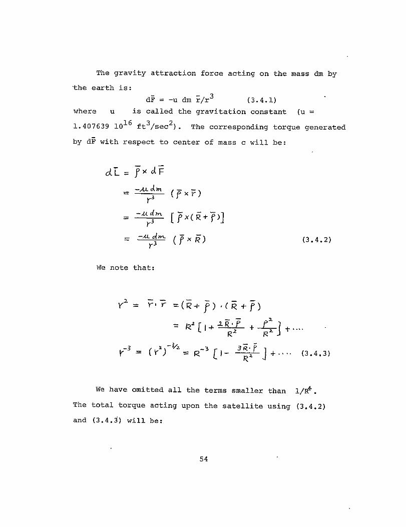
The gravity attraction force acting on the mass dm by
the earth is
dF = -u dm rr3 (341)
where u is called the gravitation constant (u =
1407639 1016 ft3sec 2 ) The corresponding torque generated
by dF with respect to center of mass c will be
-A)L r3CUn (fxP)
r
tLd (342)
We note that
2F x
- R ER shyy7 ] + (343)= -
We have omitted all the terms smaller than ii
The total torque acting upon the satellite using (342)
and (343) will be
54
L - J f fxZ m t f3(t)_X)=--5 [ R2 R3 g2
By definition because c is the center of mass the
first term in the above equation has to be zero therefore
f kf-T OY (344)
If L is expressed in body principal axes let
PIZ (f2) Then
3Z P1 fJ + RzR f - R fR1 F3 + PzLf +
tRI~+ RU+ Rpyy 3
Using the fact that in body fixed principal axes all
the cross product moments of inertia are zero
We have therefore
Lq = -WT R3 (I --s ) I 345) F1 RAZ(Ty - )l
55
In vector notation
- 3_ A (346)
where
Mis the matrix of
i _moment of inertia
and
x = f ( P i
(346) is the equation for the gravity gradient torque
it has a simple format
2) Order of magnitude considerations
Since GGT is the major disturbing torque for satellite
attitude motion it is important to know its order of magnishy
tude As a matter of fact this information - order of magshy
nitude - plays an essential role in our analysis of the dyshy
namics by asymptotic methods
From orbital dynamics [37] the magnitude of the posishy
tion vector R can be expressed in terms of eccentricity e
and true anomaly f that is
q -(347)
56
where a is the orbit semi-major axis The orbit period
p is
- -(348)
Combining (346) (347) and (348) we have
6 3 dost (14P6Cc4T2 rPI
(349)
We can say that the GGT has the order
of the square of the orbital frequency if the eccentrishy
city e is far from one (parabolic if e=l) and if the moment
of inertia matrix Im is not approximately an identity matrix
(special mass distribution)
3) Re-grouping Terms for GGT We find that Rb - the orbital position vector expresshy
sed in the body fixed coordinates - contains both the orbital
and the attitude modes Inspecting the GGT equation
(346) it seems possible to group the orbital and the attishy
tude modes separately
Since
R (
where i denotes perigee coordinated we write
57
-6 R C kgt CZN RA
--= 3 X -IM Cnb
(3410)
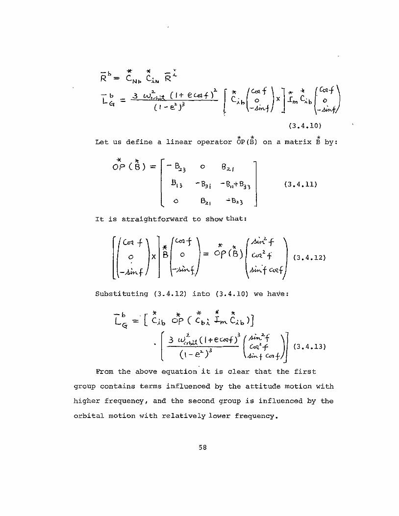
Let us define a linear operator OP(B) on a matrix B by
-X -) -
A -B 3i -+B33 (3411)
B -B- 3
It is straightforward to show that
oI+ degPPe I-t - Gi xlV Jc(B~)(C+ )(3412)
Substituting (3412) into (3410) we have
-b = cbo~ b t Z ~ )6-)- - X XLGC 6C OP(Cb nxkmCl6
2 33 CU(l+ecQ) 3
bull -r- 1(3413) 0 -f gtm
From the above equation it is clear that the first
group contains terms influenced by the attitude motion with
higher frequency and the second group is influenced by the
orbital motion with relatively lower frequency
58
(B) Geomagnetic Torque
A satellite in orbit around the earth interacts
with the geomagnetic field and the torque produced by
this interaction can be defined as a vector product
L VMXS (3414)
where 1 is the geomagnetic field and VM is the
magnetic moment of the spacecraft The latter could
arise from any current-carrying devices in the satellite
payload as well as the eddy currents in the metal structure
which cause undesirable disturbing torques On the other
hand the vehicle magnetic moment could also be generated
purposely by passing an electric current through an
onboard coil to create a torque for attitute control
If the geomagnetic field B is modeled as a dipole
it has the form [38]
i L~ze- (3415)RZ)
where i is a unit vector in the direction of the
geomagnetic dipole axis which inclines about 115
degreesfrom the geophysical polar axis Vector R
represents the satellite position vector 4AS is the
magnetic constant of the earth ( S = 8lX1i02 gauss-cm )
59
Combining equations (3414) and (3415) and expressing
in body fixed coordinates we have
-v)j j6iae5 (ePSF4)RA]
(3416)
Although neither the geomagnetic field nor
the body magnetic moment can be determined precisely
in general modeling both of them as
dipoles will be sufficiently accurate for our purpose
Summary of the Section
1 Gravity gradient torque (GGT) and geomagnetic
torque (GMT) are by far the most influential disturbing
torques on satellite attitude motion
2 The basic equation for GGT is
4 -r -X]J R (346)
For G1jT is
tM ( Ci b 3 -8 3 B shy
(3416)
60
3 GGT and GMT have the same order
as Worbit if the eccentricity is not too high
and if the satellite mass distribution is not too nearly
spherical
4 By re-grouping we separated terms of attitude
frequency and terms of orbital frequency in L q and Li
the results are (3413) and (3416)
61
35 Asymptotic Approach for Attitude Motion With Small
Disturbances
(A) Eulers equations
Eulers equations in vector form are
LO x f- Tj t 5 1) + times] j Tz shy
assuming the initial condition is
where e2 F rz +plusmn represent the disshy
turbing torques The order of magnitude of these disshy
turbing torques are discussed in the previous section The
small parameter E is defined as the ratio of orbital
and attitude frequencies
Let WN() be the torque-free Kirchhoffs
solution which satisfies the particular initial condition
that is
t 0 EIM N+(JX] Ir tON =n0 (352)
By Enckes approach [37] let
+ (353)
62
substituting (353) into (351) and subtracting
(352) we have the equation for SW(i)
Sj+ 4 1 k Wo IMI W-C + [ix
+i- [j -_ +cxTZ
(354)
Note that Enckes perturbational approach is not an
approximate method Because by combining (354) and
(352) the original equation can be reconstructed
Nevertheless performing the computation in this perturbashy
tional form one has the advantage of reducing the numerishy
cal round-off errors
For simplifying the notation a periodic matrix
operator Att) with period of Tw can be defined as
A ) -t [( X) r u (355)
Eq (354) can be re-written as
-x -I
-w Act CLd + ~(i~)t S
(356)
63
We see that the above equation is a weakly non-linear
equation because the non-linear terms are at least one
order smaller than the linear ones
Further by Floquet theory a linear equation with
periodic coefficient such as A() in (356)-can
be reduced to a constant coefficient equation as
follows
Let matrices IA and A() be defined as
PA Tvf ~ATW )
~(357)
A ( c(t) -RA
PA (=
where iA (a) is the transition matrix for A(t)
It can be proven that [36] 1 amp-i
(i) A t) is a periodic matrix
PA(-) t+ T) PA
A(t) PA(-) +I P-1
= A a constant matrix
64
Let W(t) be transformed into LMC) by
lit PFA() 8W (358)
Then
= PA w+ PA tv
- AG __shy PA t4 PASAWP+ T+ i+
PA -I P4 - X PAR A - ( - I XPA -)CX
-
4 4 ---S LV -amp 1 -AP 2hi+ (359) PA I
These results can be proved by using eq (355) and
the property (2)
Moreover in our case the constant matrix RA
is proportional to IT therefore it can be considered
to be of order E Also for simplicity RA can
65
be transformed into a diagonal (or Jordan) form
S-uch as
I ) - 0 0
0 0 (3510)
0 L3
Let
l--Md-- (3511)
Substitute X into (359) finally we have
-x A -1 -I c I
-- QJ -j+e- + ) (3512)
where
ampk=W-PA x (3513)
66
MTS Asymptotic Solution
For solving (3512) we apply the linear multiple
time scales asymptotic technique [3] We first expand
the time domain into a multi-dimensional space)
and o IC etc are defined as
The time derivatives in the new dimensions are
transformed according to
A 4 d ___7I j_ +
(3514)
a-CO0
Also we assume that the dependent variable U-t)
can be expanded into an asymptotic series of a
v() Oampt-ot-1-)-- ThecxV (3515)
67
Substituting (3514) and (3515) into (3512)
we have
M rt
0 xO O-2- J-F- (3516)
By equating the coefficients of like powers of S on
both sides of (3516) we have
Coefficient of i
+cent (3517)
Coefficient of
68
Coefficient of
2- a--4 r
L t ] + T (3519)
Solving the partial differential equation (3517)
we have
o(3520) =
where u is not a function of r and the initial condishy
tion is
1J (o) = 0
and amporij Z- ) is yet to be determined
Note (3520) implies that the zeroth order solution
for Eulers equation with small disturbances is the
Kirchhoffs solution
Substituting (3520) into (3518) we have
a TCO 0)T
+ aT (3521)
69
This equation with the initial condition 0j(0)= 0
can be solved as
4ITO -X
4JTIamp (3522)
-I1 The term q x in the above equation
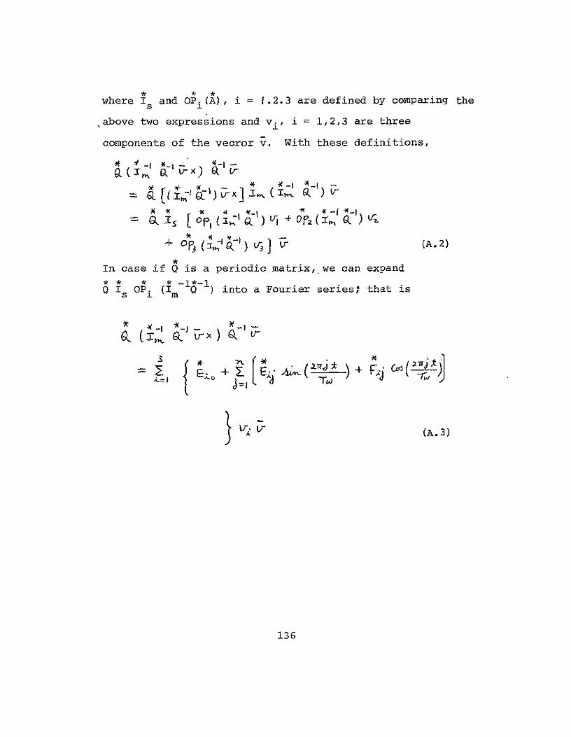
can be written as shown in Appendix A as followsshy
-
F 3+ series
O(3523)
where P1 2 and 3 are periodic matrices
with period of lb and ~ 2~3~ are three
components of the vector tJ if we expand F
F and F3 into Fourier series
70
we have
3 Xn A
(3525)
where EIj and F-I are constant matrices
Also in case that the external torque TI is not an
explicit function of time then Q-T1 can be transformed
into a particular form as
(3526)
where are functions of slow variables
onlyand tp (t 0 ) is a fast time-varying
function The expressions of (3526) for gravity gradient
torque and geomagnetic torque are given in the following
sections
Substituting (3525) and (3526) into (3522)
71 F WI 4 (r-j(I AI
71
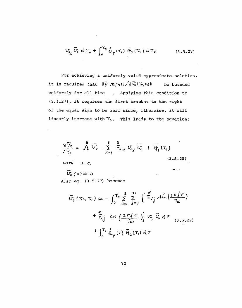
For achieving a uniformly valid approximate solution
it is required that (tfl)[II UstoUoII be bounded
uniformly for all time Applying this condition to
(3527) it requires the first bracket to the right
of the equal sign to be zero since otherwise it will
linearly increase withTr This leads to the equation
A V X Fxc bU L4 TtO)1
(3528) Wurh C
Also eq (3527) becomes
(27T4 (3529)
72
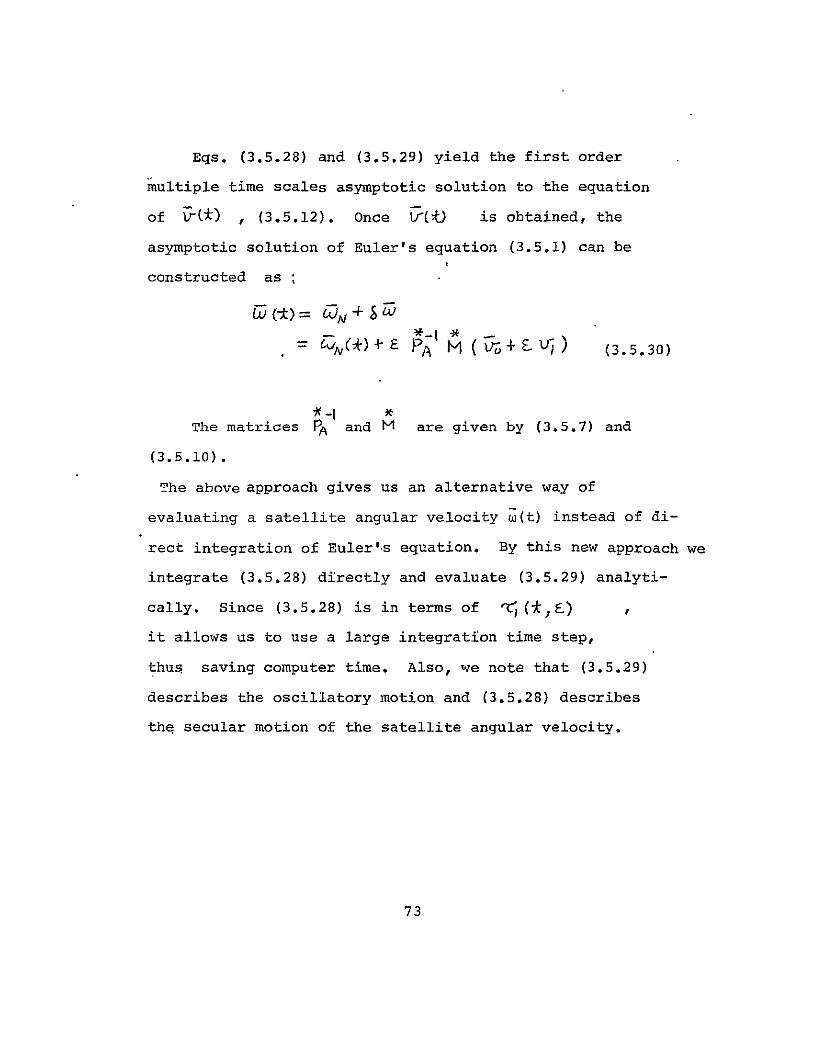
Eqs (3528) and (3529) yield the first order
multiple time scales asymptotic solution to the equation
of 1(t) (3512) Once Lt) is obtained the
asymptotic solution of Eulers equation (351) can be
constructed as
WFt) 0 S
( +E PA +F-V) (3530)
The matrices A and M are given by (357) and
(3510)
The above approach gives us an alternative way of
evaluating a satellite angular velocity w(t) instead of dishy
rect integration of Eulers equation By this new approach we
integrate (3528) directly and evaluate (3529) analytishy
cally Since (3528) is in terms of i (Fa)
it allows us to use a large integration time step
thus saving computer time Also we note that (3529)
describes the oscillatory motion and (3528) describes
the secular motion of the satellite angular velocity
73
(B) Solution For Euler Symmetric Parameters
Euler symmetric parameters are kinematically related
to the angular velocity by a linear differential equation
(329)
- L I V (3531)
Hence
=N (3532)
Again by linear multiple time scales method
To=
we have
a iLft (3533)
74
Assume that
jS(~ (3534)Ott 1930c t3 i +
Substituting (3533) and (3534) into (3532)
and arranging terms in the power of e we have
Coefficient of 6shy
2Co (3535)
Coefficient of L
plusmnPL-~[ N o (W] 0 (3536)
Coefficient of pound2
-= 3j--2 92 2- -t j(JN3 shy
(3537)
Let be the transition matrix for
2 7Jthat is
The expression for 0) is given by
(3329) that is from the solution of 1 by Mortons
75
approach Similarly I (tjko) can be also achieved
by using the Floquet theorem although the latter one
is more numerically oriented and requires several transshy
formations
The solution for the S order equation (3535) is
-eL--C) = _To (-CCNTd--) (3538)
with IC
and PON (Z) is yet to be determined
Substituting eq (3538) into (3536) we have
7o z 1 O
(3539)
The solution to the above equation is
plusmnpftQ r 4tf stw) 0 oljPONr 067) 0(o)
(3540)
where S (trr) given by (3530) is afunction
76
of and It I Oand to (4o) is a function of t5
only By re-grouping terms it is possible to write
I0I4 4 o as follows (appendix B)-
o
~
(3541)
Substituting (3541) into (3540)
3= Campo0 r 0ICo R(1)PONC) -c
-r Pa(r) R2U(l pIN (L) dj (3542)
In order to have 1lfi11ll1oI 1 bounded in- it is
necessary that should not increase with time
faster than Therefore in eq (3542) those
terms which increase linearly with rhave to be set to
zero That is
R -CI PO -C j( ) (3543)
and (3542) becomes
(3544)
77
Equations (3543) and (3544) give an asymptotic
solution to the equation of Euler symmetric parameters
1 CC1) C 0 ) PPN tri) + j 3 ~o 1 )+S (3545)
where Pa from (3543) gives the secular
variation of the perturbational motion and
gives the non-biased oscillatory motions
Summary of the Section
(A) The rigid body satellite attitude dynamics
are described by
- j + fwx] W pounde T+ (351)
iS = -i (3531)
which can be replaced by the asymptotic approximate
formulation
A u- X FV gt u + Q-) (3528)
bEA =1 ~o jT
- 4ofamp-) -(-yd (3529)
78
W-+E PA ) (3530)
tC1 (3543) 2(Tho Y
(3544)
(3545)
(B) The secular eqs (3528) and (3543) have to
be integrated in C ( t $) or equivalently in
a very large time step in t The oscillatory equations
(3529) and (3544) can be analytically calculated if
the external torques -T are not explicit functions of
time
36 Attitude Motion With Gravity Gradient Torque
The gravity gradient torque given by (3413)
is
(361)
79
where e f and t are the satellite orbit
eccentricity true anomaly and averaged orbital angular
velocity respectively OF is a linear operator given
by eq (3411)
From (3330)
i =C 1 Czqz2t) + C (2Rt) + C3 (362)
and
o Cz2 (2Pt ) += )V Cn (2Zt) + C h A C3 CIh
C C c(2P(Cz Ch d)RC3I +k)t)
(363)
where C1 C2 and C3 are three periodic matrices
with period of TW
Substituting (363) into (361)
- i)t - x
A 4t T
- CI-ThC c) Cr3 )t80CL -+C2_ Cv2It4+ o Csl c1)tC
80
2shy
+ op1c4Ict cr1 4je)AA2z- 4)e )
3 Ihe-el)
CeJZ
+or (C2( Jm C CTt + 6shy
6 C
a SP() + Sj() ~a~~(~)+ S3 (4) LC2s~Rt)
+ S ) 4 vt tfrt) + St Ct (4Rt)
4~~~~~~~a S6amp ~(6RfyJAL )+S~
6Z C3 Or C1 1h Ci 4 cl X z 3 )
81
Because i 7 are periodic matrices
with period TW they can be expanded into Fourier
series with period of T That is
TTW
(365)
With that G LT can be expressed in the form
L C Cx 4X+ p(Xo) GL(tCl)(366)
2 3
r(1)=3 WtWu (I+ C4ck) I 4A 24
) A (367)
T (368)
82
QM7a CO (ZIT4)+ f 7 JA(d ~ cl
(369)
and amp(LuLtt) can be analytically integrated
Resonance ITT
In special cases if the tumbling frequency-n and
the polhode frequency R are low order commensurable
that is there exist two small integers n and m such
that
= o (3610)
then resonance will occur For handling resonant situations
for example if aI - 2 =o then in equation(369) cof terms such as 4 2 Pt )-r 2iz j
etc will produce constants (ic A ztt rw -I_ -cz-d4ft cad = ) These constants should
be multiplied by Q) and grouped into -j in (366)
Then our theorywith the same formulation enables us to
predict the attitude in the resonant case as well
83
A Numerical Example
A rigid body asymmetric satellite in an elliptic
orbit is simulated Here we assume that the satellite
attitude motion is influencedby the earth gravity gradient
torque only
The numerical values used in this example are the
following
Satellite moment of inertia
IX = 394 slug-ftt
I =333 slug-ft2
I = 103 slug-ft
Orbit parameters of the satellite
eccentricity e = 016
inclination i 0
orbital period = 10000 sec
Initial conditions are
Wx = 00246 radsec
WV = 0 radsec
b = 0 radsec
Satellite starts at orbit perigee and its initial
orientation parameters are
0= 07071
S= 0
p =0
p =07071
84
In this case the small parameter S is about
W acrbJt 0 3 w attitudle
With the above initial conditions the satellite attitude
dynamics are first directly integrated using a fourth
order Runge-Kutta method with a small integration time
step size of 10 sec for a total interval of 8000 sec This
result is considered to be extremely accurate and referred
to as the reference case from here on The other simulations
are then compared to this reference case for
checking their accuracy A number of runs have been
tried both by asymptotic approach and direct integration
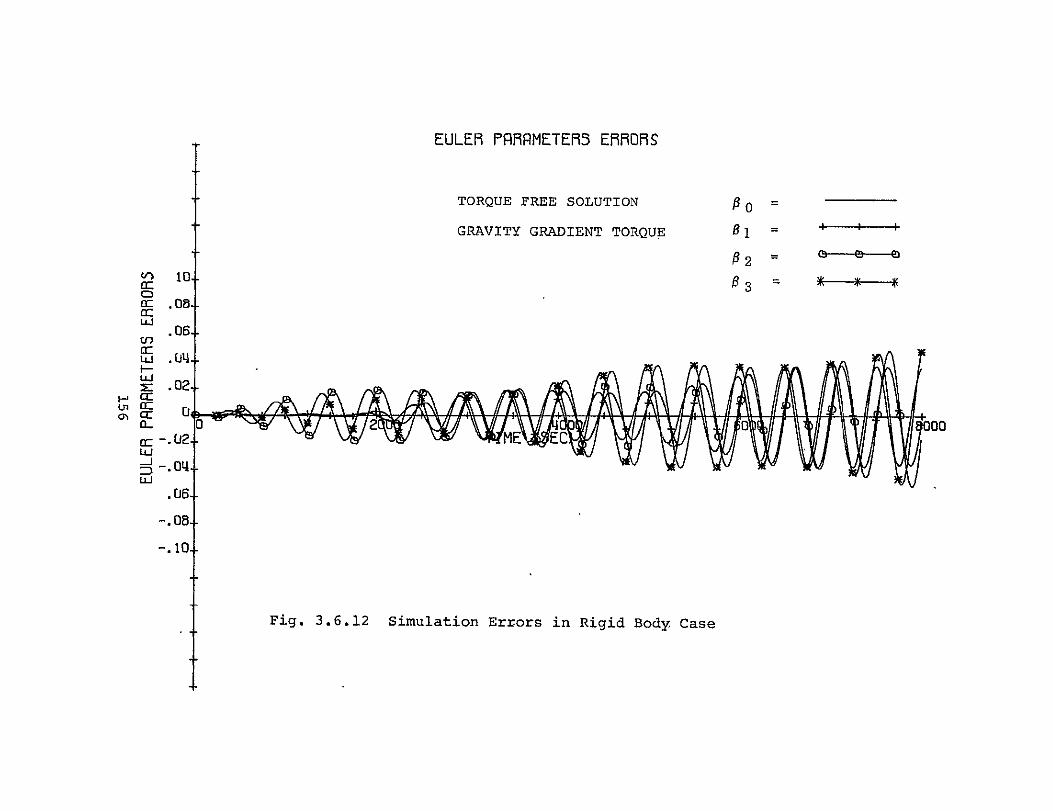
with different time step sizes They are summarized in
Table 351 The errors in each case - ie the differences
between each simulation and the reference case - are
plotted in terms of time and given by Fig 361 through
Fig 3612 Fig 3613 is a plot of the maximum
numerical errors as functions of the step size From
this plot we see that with direct integration the
step size AT should be no greater than 25 sec On the
other handfor asymptotic simulation the step size can
be as large as 500 sec although the first order asymptotic
85
approximation errors approach zero as pound -gt 0 but not
as mt- 0 Fig 3614 is a plot of the required
computer time in terms of the step size AT We note
that for extrapolating a single step the asymptotic
approach requires about double the computer time using
direct simulation However since the former
allows use of a large time step overall this new approach
will have a significant numerical advantage over
direct simulation In our particular case the saving
is of order 10 Although in this comparison we did not
include the computer time required for initializing an
asymptotic approach by calculating Kirchhoffs
solution and some Fourier series expansions etc we
argue that this fixed amount of computer time
required for initializing (about 40 sec for
the above example) will become only a small fraction of
the total if the prediction task is long For example with
theabove data if we predict the satellite attitude motion
for an interval of three days the direct integration
with a step size AT = 20 sec requires 1700 sec of computer
time1 while the new approach with 6T = 500 sec needs
about 170 sec plus the initialization of 40 sec
86
--
37 Satellite Attitude Motion With Geomagnetic Torque
The geomagnetic torque acting on a satellite can
be written as (3416)
(371)
where 6 is the vehicle magnetic moment and
e is the geomagnetic dipole axis The latter
for simplicity is assumed to be co-axial with the
earth north pole
Substituting the expression of Cjb from 6--6
(3330) into LM we find a LM can be written
in the form of
LM - (--O) G V) (372)
where
6LP (-ED) = ( X)C b
r_ xtX Coo (i-t) + Cz 6 ( 2 Rzt)tC
Jt 3 ( efRA
(373)
87
By expanding C1 cJ cJ into Fourier series
we see that ampLM can be analytically integrated in terms
oft 0 Eq (372) corresponds to (3526) in section 35Co
and the asymptotic formulations can be easily applied
Numerical Example
A rigid body satellite perturbed by the geomagnetic
torque is simulated with the same satellite which flies in
in the same orbit as given in section 36 In addition
we suppose that the vehicle carries a magnetic dipole V
which is aligned with the body x-axis
At mean time the value of the geomagnetic
field is assumed to be
= 5i~i Io S - a ~
Using the above numbers we simulated the satellite
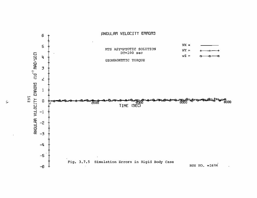
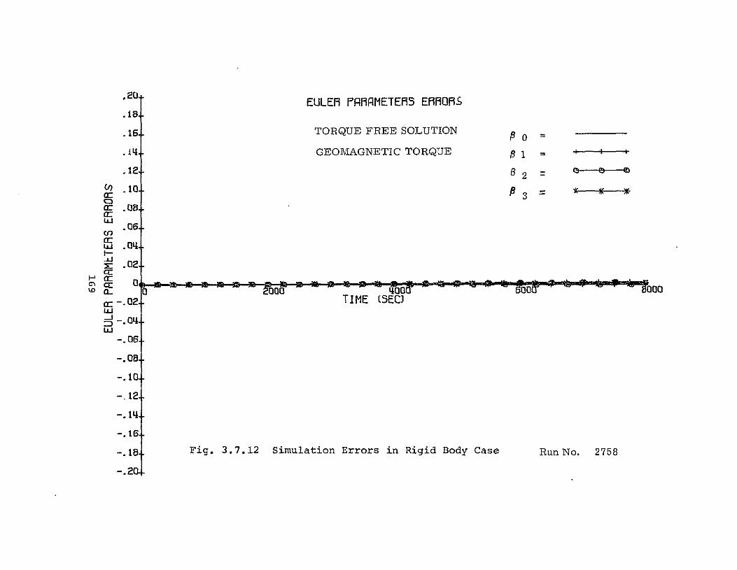
dynamics by direct integration and by the asymptotic
approach Table 371 lists all the runs tried The
errors of each case are plotted in Fig 371 through
Fig 3712 Similar conclusions as given in the gravity
gradient case can also be reached for the case of geomagshy
netic torque
88
CHAPTER 4
PREDICTION OF ATTITUDE MOTION FOR A CLASS OF DUAL SPIN SATELLITE
41 Introduction
In chapter 3 a technique for speeding up the preshy
diction of a rigid body satellite attitude motion was
developed However the limitation that requires the
satellite to be a rigid body seems severe because many
satellites in operation today have one or several high
speed fly-wheels mounted onboard for the control or
stabilization of their attitude motion The combination
of the vehicle and its flywheels sometimes is referred to
as a dual spin satellite Therefore it seems desirable
to expand our prediction method for handling the dual
spin case as well In doing so it turns out that-it
is not difficult to modify our formulations to include
the dual spin satellite if the following conditions
hold
1 The angular velocity t is a periodic function
when there is no external torque
2 A torque-free analytic solution of the system
is possible
3 External torques are small
However the dynamic characteristics of a dual spin
89
satellite in general are not clear yet as far as conditions
one and two are concerned Although we believe condition
two might be relaxed by some further research they are
beyond the scope of this effort
As a demonstration examplefor handling a dual spin
case we consider a special class of dual spin satellites
that is a vehicle having a single fly-wheel which is
mounted along one of the vehicle body principal axes
The satellite is allowed to have an arbitrary initial
condition and to move in an arbitrary elliptic orbit
In what follows the rotational dynamics of a dual
spin body are first discussed An excellent reference
on this subject is by Leimanis [22] Later the torque
free solution - which serves as a nominal trajectory shy
for a class of dual spin satellites is presented This
torque-free solution was first given by Leipholz [23]
in his study of the attitude motion Of an airplane with
a single rotary engine Then in section 44an asymptotic
formulation for a dual spin satellite is discussed and
two sets of numerical simulations are presented
90
42 Rotational Dynamics of a Dual Spin Satellite
For a dual spin satellite we assume that the
relative motion between fly-wheels and the vehicle do
not alter the overall mass distribution of the combination
Thus for convenience the total angular momentum of
the system about its center of mass can be resolved into
two components They are H the angular momentum
due to the rotational motion of the whole system regarded
as a rigid body and H the angular momentum of the
fly-wheels with respect to the satellite
The rotational motion of a dual spin satellite
is therefore described by
I I
dt (421)
where Im is the moment of inertia of the combinashy
tion (vehicle and wheels) and M is the external
disturbing torque
Applying Coriolis law we can transfer the above equation
into body fixed coordinates b
-b IZ b++ -h j1
6 (422)
91
Further by assuming that the wheels have constant
angular velocities with respect to the vehicle
o0
Hence
- -( x) (423)
This equation is equivalent to Eulers equation
in a rigid body case
For satellite orientations because Euler symmetric
parameters and the angular velocity 0 are related
kinematically the equation remains the same for a dual
spin satellite that is
O( _ I (424)
ck
43 The Torque-free Solution
The motion of a dual spin satellite with a single
fly-wheel mounted along one of the body principal axes
can be analytically solved if there is no external torque
acting on the vehicle
92
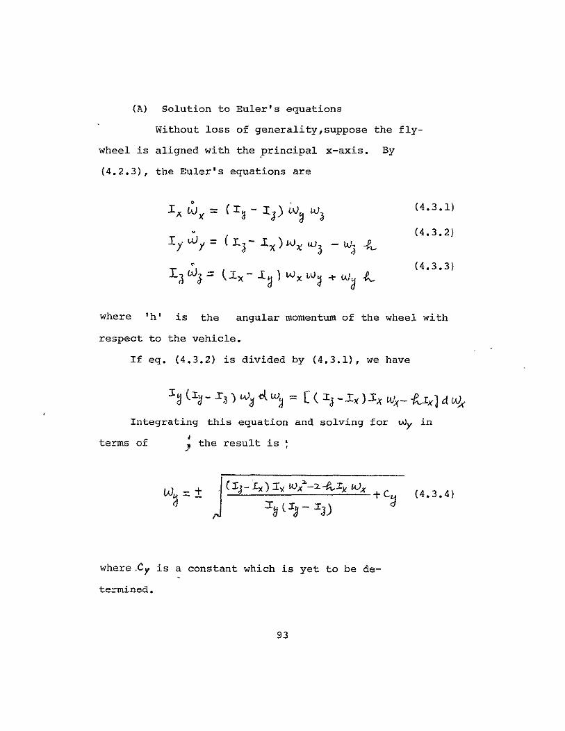
(A) Solution to Eulers equations
Without loss of generalitysuppose the flyshy
wheel is aligned with the principal x-axis By
(423) the Eulers equations are
L(431)= Wi Ki=( 3 ~
to (432)Iy LWX
(433)
where h is the angular momentum of the wheel with
respect to the vehicle
If eq (432) is divided by (431) we have
X)yiW~ W g)x W4-ampix d4
Integrating this equation and solving for Wuy in
terms of the result is
+C=t Xe k -V (434)
where Cy is a constant which is yet to be deshy
termined
93
Similarly using eq (433) and (431) LA can
be also expressed in terms of L)x the result is
- (3X--y)XWW242z~ Ii+ C3 (435) Tj (L-1y-T3)
where C is another constant
In case that there is no external torque we know
that the rotational kinetic energy T and the total
angular momentum HT of the system must remain constant
ie
(436)and
(x~amp~q~jL+ jy LU+ lt=H (437)
Equations (436) and (437) can be derived by integrashy
ting (4W3) +w 4- 3a) + W$ 33)]3
and
respectively
94
Having determined the angular momentum HT and kinetic
energy T one can calculate the constants cy and cz
by substituting (434) and (435) into (436) and
(437) they are
(438)
or W) and W can be rewritten as
(439)
where
p A J shy
- = - c J S 5 WA 4 x
(4310)
To find X one can use (439) the solutions
Ut and Wj with (-431) to eliminate WY and
95
VO3 such that an equation for can be obtained
dw (4311)
Orx
) W4) ply (43-12) 2 P7
Suppose that -y p3 has roots of W 1 pound02 WA)
and LxA) in a descending order then
Jd ) I x
t4a3J13)
This integral can be easily transformed into an
elliptical integral ie eq (4313) is equivalent to
IJ- W (4314)
where
2rI (4315)1-n Q Y rj
Ixh j (W _42Ty L - 0-94
W (4316)
96
and if 144 lt poundV(o) _SUJ3 ) then
]X4 - 1(U+ W)w(W w 3 (4317)
and if tQ ltW- JI then
W- -O=(ww W4 j(4318)
(B) Euler Symmetric Parameters
Since the equations of Euler symmetric parameters
remain unchanged whether a space vehicle has fly-wheels
or not
~I12jjjj(4319)
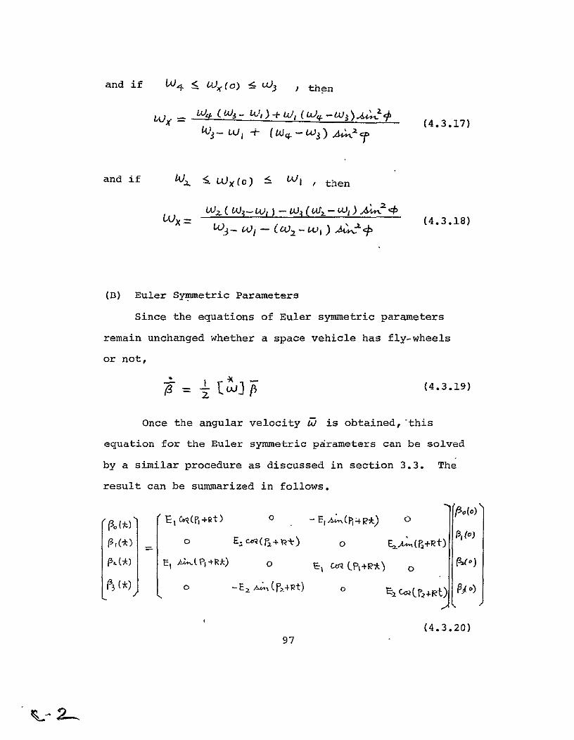
Once the angular velocity tD is obtained this
equation for the Euler symmetric parameters can be solved
by a similar procedure as discussed in section 33 The
result can be summarized in follows
Po(o)f3j((t 0
0~t Eca-C F+ 14t) a E AM-(gRt)2 131o)
E1 At(I-R) 0 E--Ctrq~ (ampJo)
0 -E4(P4Rt) 0 ~ c4 2 R)~o
(4320) 97
where
- = fH-plusmn+Y y) I
ViT -4-Iy WampJo)
SHT - ly W ()
= oS- -r--)-R-
E =ost ()-Rt -r ( -r-P=
and
Z-TW4wxIt(-) - 0k
50-HITr4 Ly Uy
t(Y (2T-HTWy-ttWO) Olt Hr - -y WY
98
TT(W and t() are two elliptic inteshy
grals T and HT are the kinetic energy and angular
momentum of the system and they are given by equations
(436) and (437) TW is the period of
the angular velocity W and h is the angular momenshy
tum of the fly-wheel with respect to the vehicle
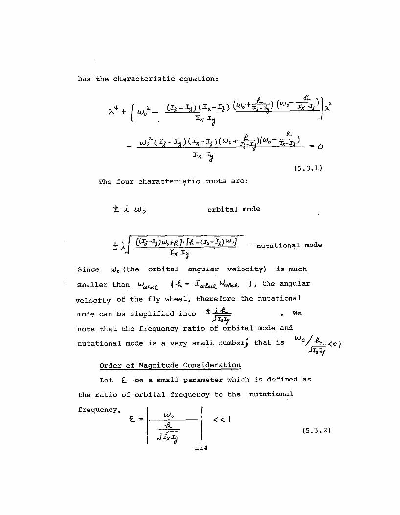
44 Asymptotic Solution and Numerical Results
Once the torque-free nominal solution for a dual
spin satellite is obtained the basic procedures of the
asymptotic approach described in section 35 for a
rigid body satellite can also be applied to a dual
spin case In order to include the gyro effect due to
the fly-wheel a few equations in section 35 have to
be changed
Equation (351) has to be replaced by
Lwx [Tn w =eT 4 z
(441)
where HL is the angular momentum of the flywheels
with respect to the vehicle
Equation (352) is replaced by
0(442)
99
and equation (355) has to be changed
I Lox-iti )YT_ (XW4 kwy(J (443)
Of course WtMt) and the transition matrix
t (1 0) arise from (439) (4317) and (4320)
They are the reference trajectory for a dual spin case
Numerical Simulations
For demonstrating the correctness and accuracy of
predicting the attitude motion in the case of a dual
spin satellite we select a numerical example with the
following data
Satellite moment of inertia
I = 30 slug-ft
1 = 25 slug-ft
1 = 16 slug-ftZ
A fly-wheel is mounted along the body fixed x-axis
of the vehicle with an angular momentum h with respect
to the vehicle
h = 02 slug-feSec
We assume that the satellite is in an elliptic ic
orbit with
eccentricity e = 016
inclination i = 0
orbital period = 10000 sec
100
The initial conditions are
Angular velocity J(O)
WX = 003 radsec
wy = 001 radsec
LU = 0001 radsec
Euler symmetric parameters (o
= 07071
= 01031
= 01065
Ps = 06913
For these numbers the small parameter E of the
problem defined as the ratio of orbital and attitude
frequencies is about
a orbital frequency Zii oOO shyattitude frequency ZT )67o
This dual spin satellite is first assumed to be
disturbed by the gravity gradient torque only The
dynamics are simulated both by direct integration and the
asymptotic approach The results are summarized in
Table 441 Also the simulation errors are presented
in Fig 441 through 4410 they are given in the same
way as in section 35 for a rigid body satellite
101
Next the dual spin satellite is assumed to be
disturbed by the geomagnetic torque only A magnetic
dipole is placed onboard with a strength of -fl
(300) ft-amp- sec which interacts with the earths
magnetic field of strength
i Z2 zXo 10
SeA- o-nf
Similarly the attitude dynamics are simulated by
direct numerical integration and the asymptotic approach
The results are summarized in Table 442 and Fig 4411
through Fig 4420
Conclusion
These two sets of data one for gravity gradient
torque the other for geomagnetic torque show that
our asymptotic approach is equally useful for a dual
spin satellite as for a rigid body case if the conditions
listed in section 41 can be satisfied The numerical
advantage of saving computer time and the approximation
error introduced by our asymptotic approach are of
similar character as discussed for a rigid body case
The details are not repeated again
102
CHAPTER 5
DESIGN OF A MAGNETIC ATTITUDE CONTROL SYSTEM USING MTS METHOD
51 Introduction
The interaction between the satellite body magnetic
moment with the geomagnetic field produces a torque on
the satellite This torque however can be harnessed
as a control-force for the vehicle attitude motion
By installing one or several current-carrying coils
onboard it is possible to generate an adjustable
magnetic moment inside the vehicle and thus a control
torque for the satellite This magnetic attitude control
device using only the vehicle-enviroment interaction
needs no fuel and has no moving parts it may conceivably
increase the reliabiltiy of a satellite In recent years
it has received considerable attention
To design such a system nevertheless is difficult
because the control torque it very small 8ince the elecshy
tric currents available to feed through the onboard coils
are limited the magnetic torque generated in
this way is not large enough to correct satellite attitude
motion in a short period of time In fact it is realized
that one has to depend on the long term accumulating
control effort of the geomagnetic interaction to bring
103
the vehicle into a desired orientation For this reason
the system can not be studied readily by classic control
design techniques
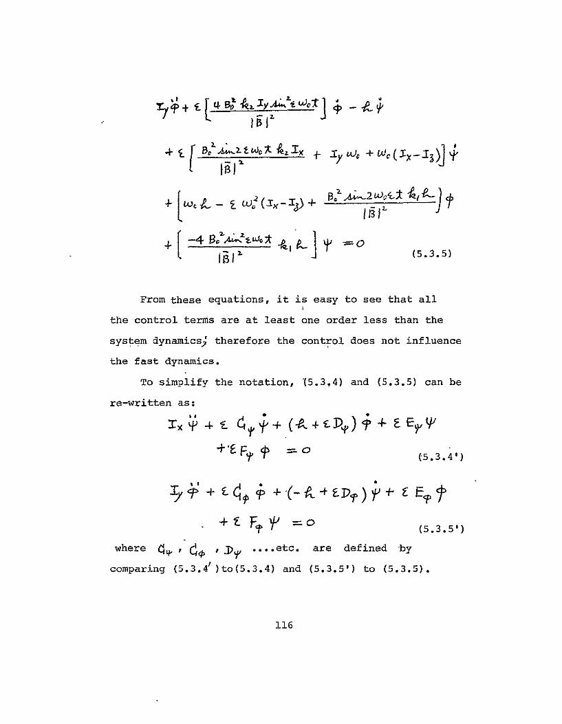
However this problem can be more efficiently
analyzed in terms of the slow variational equation
from the MTS approach By casting the dynamics of the
above system into an 4TS formulation the fast motion
(attitude nutational oscillation) and the slow motion
(amplitude variation of the nutation) can be separated
Even though the effect of the magnetic torque on the
dynamics is very difficult to observe and comprehend in
real time t still using the slow secular equation
in terms of a slow clock the control effect on the
nutation amplitude change immediately becomes transparent
In this chapter we will analyze a magnetic attitude
control system for a dual spin earth-pointing satellite
For more imformation the reader may refer to the works
of Renard[39] Wheeler [40] and Alfriend [41]
52 Problem Formulation
The Problem
A dual spin satellite moves in a circular orbit
its antenna is required to point toward the center of
the earth A momentum wheel is assumed to be mounted
104
POORi ctI
along the satellite pitch axis for control of the
pitch motion
quatorial plane
planeorbit
Fig 51 Roll yaw and pitch axes
For the above satellite a roll-yaw oscillation
called nutation is possible This is because its
angular momentum vector may not be perfectly aligned
with its angular velocity vector due to external disshy
turbance or initial misalignent etc
A magnetic control device using the geomagshy
netic interaction is to be designed to damp out
the nutational oscillation as well as to keep vehicles
105
angular momentum perpendicular to the orbit plane
Equations of Motion
The Eulers equations for a dual spin satellite
are given by (423) they are
t- -t T W3- (521)
where th is the angular momentum of the fly-wheel
and M is the external torque on the vehicle
Assuming 1 c and e are the Euler angles which
correspond to yaw roll and pitch for concatenated
Y-WI- z rotations indicated by
trajectory)
frame rotation about X rotation about (xyz)- ------ ---
by amount of ICbody ---------shyby amount of C P
rotation about z _frame) (x z z ) ------------
by amount of (x y
Then a kinematic relation between the angular veloshy
city and the derivatives of the Euler angles can be
written as [42]
106
- e4e~ 1 + t t E- (522)-
where ti are unit vectors egA is in the
direction of vehicle position vector and P- is normal
to the orbital plane The term (cct) es describes
the rotation motion of the satellite in a circular orbit A A
Transforming e( e and ejl into the body
fixed coordinates and using small angles assumption
equation (522) can be written as
++ + q
(523)
(44 - (524)
S+wo
Substitute (524) into Eulers equation (521)
we have
107
GR M(525)
Earths Magnetic Field
The geomagnetic field B can be approximately
represented by a magnetic dipole as discussed in section
34
_-- te(Y (526)erNB- ]
where s is a constant of the geomagnetic field
( tA = 81 x 10 gauss-cm ) 98 is the unit
vector along the dipole axis and R is the vehicle
position vector Using Fig 51 can be expressed
in the axes of e e e (called trajectory
axes)
A 4C CPJ (527)
wherei is the inclination of the orbit Substitute
(527) into (526) we have
A
+ A ej3 (528)
108
Further because the satellite is in a circular orbit
and if the vehicle is well controlled the body axes of
the satellite should be closely aligned with the trajacshy
tory axes therefore
6Sb B w tta -2 4 LWot AAA
CzOWt 2A
or
(529)
-b6 - -1B0Aw 0 t 5oOA4 oo
Co O~ (529)
19 ol IAIL
w-log
The Control Torque
Assuming M to be the magnetic moment of the
vehicle the torque experienced by the satellite due to
the geomagnetic field is
(5210)1
For the control of the vehicles attitude let us preshy
specify the control torque M as
MaeA represents a desirable control law
which may not be possible to implement P
is two-dimensional because the pitch motion is controlled
by the momentum wheel which is excluded in this analysis
The first term in the above equation -(( j3y
reflects elimination of excessive angular momentum due
to the perturbed vehicle body rotational motionand
thus damps the nutational motion The second term
is to control the vehicle orientation through the gyro
effect of the momentum wheel
Let us take the cross product of equation (5210)
by B
110
13 = B ( )
=I~ VM B (VW ) (5212)
The above equation may be satisfied if we pick
V (5213)
In this case will be perpendicular to B and
also to M It can be proved that this VM is
the smallest magnetic moment required for generating a
known torque M Substitute (5211) into (5213) to
give
lI B (- Iz - t (5214)
We see that V is three dimensional Thus in
order to implement the above control law it requires
three electric current-carrying coils and their suppleshy
mental equipment to be mounted orthogonally to each other
in the vehicle
However let us suppose that there is a weight and
space restriction We have to limit ourselves to use
one coil only By putting a single coil along the pitch
i1i
axis the first and second components of equation
(5214) are eliminated the control law now is
-b -- i o
(5215)
The corresponding torque generated by this control
law will be
(5216)
By substituting (5216) and (529) into the equation
of motion (525) we have
J + WOt+ 4ampOdeg =W
+ 0____
1511 (5217a)
112
i
and 4 -Aigi1+S
0 ~(5217b)-qB
These equations are linear but can not be exactly
solved since the coefficients are time-varying The
quantities k1 and k2_ should be picked such that
the above system is stable
53 System Analysis
Free Response Solution
The roll-yaw dynamics (525) are first determined
without considering external torques We see that
the dynamics contain a fast nutational mode and a slow
orbital mode
The system (525) without the external torque
113
has the characteristic equation
N + [wiO - (3 I -IT-I (w-+-) CUr xj
WO T ))Li s)(Lo0 -41 r)(- X w 0 (j
(531)
The four characteristic roots are
S U orbital mode
- 1(CI- 8 )w J (k_ ixIs)wJ nutational mode
Since U4 (the orbital angular velocity) is much
=smaller than W h0 (k I L 4 t ) the angular
velocity of the fly wheel therefore the nutational
mode can be simplified into plusmn - - We
note that the frequency ratio of orbital mode and
nutational mode is a very small number that is ltltlaquojol
Order of Magnitude Consideration
Let F_ -be a small parameter which is defined as
the ratio of orbital frequency to the nutational
frequency W
(532)
114
Assume h I I and I are of order one then
the following terms are ordered as
4= oCE)
t-c = o (E)8=j- -S 44t L2 = 0( (533) 13 f aJ~tc G1 c(=oCIA)
18 ) ( e)
The control gains kI I k are limited by the small
current generating the torque and is therefore necessarishy
ly small We assume that At =-- E)
For convenience F and its power can be used to
indicate the order of each term For instance W0
will be replaced by u~o By doing so equations (5217)
are
+ pound O 2 I + 1617
Ifl x4+(I4)j$
- pound -DfAA WLoot 4k+euro_+ f
4 zL2 plusmn tt] + (534)
115
7j f B1y A t y +)
- Ic4A41 ~ 7t I b b O
iI (535)
From these equations it is easy to see that all
the control terms are at least one order less than the
system dynamics therefore the control does not influence
the fast dynamics
To simplify the notation (534) and (535) can be
re-written as
deg +9 ltP (534)
17 ltP+ E4+f
4Z Ft o (535)
where L etc are defined by
comparing (534)to(534) and (535) to (535)
116
Multiple Time Scales Approach I
For solving equation (534) and (535) we use
the MTS method as outlined in section 22 by
expanding the dependent variables and into
asymptotic series in f-
y=40 + qI + e 1 + (536)
(537)
Further the dimension of the independent variable
t (time) is also expanded into multi-dimensions as qiven
by (2211) (2212) and (2213) Expressing equations
(534) and (535) in new time dimensions we have
I-t
+ 4
ao __
0
(538)
117
and
a CP 1 O + f
( 4
4 at04 a(- 9 0 tf+ ) 4 Fo(Yo+E + )
0 (539)
By equating the terms of like powers of - in the
above equations we have
Terms of t
o+ _ o
(5310)
The solutions-are
_Txq Jj
(5311)
118
Where p q r and s are not functions to but
they may be functions of ttC-etc They are yet to
be determined
Terms of t
Tlt)Y - -C- Y --p
-5
(5312)
Y alt 2--Llt- 5v
-o and o fromSubstituting the solutions of
(5311) into (5312) we have
+ ~-+ rHNt t
(5313)
119
119
L
where
-C J -t
VY I
WY (5314)
Note - etc are all functions of t C
only And p q are yet to be determined In order thattc j and ji p j be bounded
the terms that produce secular effects in 9s t| must be eliminated Equations (5313) are
linear the transition matrix to) for andand in (5313) is
12Q
Aa Ncr0
-lpb rshy J tp( wo)
2
4 p(i 0 -))
(5315)
The solutions for with zero initial
conditions are-
121
N- ZNa
N v-N
(1 2XN Ae 2J +rL 4PAltJij t + NwY -Zlt) k1iiuta
(5316)
Notice the terms (4+1C gt ) to
and (V -7(-4 -- T_ ) will increase
linearly with time In order to have 4 P I bounded
these two secular terms have to be set to zero They
are
V+-U + - =0
(5317)
122
which are equivalent to I
-TX + (5318)
-V I r
Also using the freedom of choosing r and s
we can set -We -- Or
(5319)
Aa-CI F
Substitute for LPL etc from (5314)
equations (5318) are then
(- + NIa -TX(4+ PpFyA
XAX L)+Ng( lt-p~+ Ng (5320)
+ N) + -D41 ____Na~ - ~Jt0
(5321)
where pl and q are complex conjugate
A first order MTS asymptotic solution for (534)
and (535) thus has been constructed by using (5311)
123
that is
(5322)
where p q are given by (5320) and r s are given by
(5319) All these equations are in terms of ^C- the slow
time scale In order to make and P decay in time the conshy
trol torque has to be selected such that it forces pqrs
to zero through the slow equations The general problem in
chapter 4 (with magnetic torque) is simpler in the present
case because the perturbed motion is kept small by the conshy
trol Linearization therefore seems adequate leading to
analytical solution
Selection of Feedback control gains
We wish to select feedback gains k1 and k7
in system (534) and (535) such that the system is
stable However because the control torque is small
and the system is time-varying the effect of the control
upon the dynamics is not clear
The above problem was then cast into an asymptotic
formulation By the MTS method an approximate solution has
been achieved as given by (5322) through which
the design problem can be interpreted in a more convenient
way That is because the approximate solution (5322)
describes a constant frequency oscillatory motion with
124
slowly time-varying amplitude pq and biases r s
pqrand s are functions of the control torque and are
given by (5319) and (5320) The problem can be conshy
sidered differently in that the control torque is used
to force the amplitude p q and biases r s to zero
In this way since the fast nutational oscillation has
been separated out the selection of the feedback gains
kf-and k_ in the slow equations (5319) and (5320)
becomes much easier
The solution for p (PC) [ or q(-tj )] from (5320)
is A __ Ix7
-- -4
+ Imaginary part (5323)
Thus p and q will approach zero if
- 4 Jtpr ltFp FyX-Jx -fli-ampfMY
where C+ F etc are given by (534) and
(535) By substitution (5322) becomes
A-wt IA4CWtR t)2
125
or equivalently for p and q to be decaying we
require
4-lt 4 (5324)
Also r and s are governed by (5319) which is
a second order linear differential equation with periodic
coefficients The necessary and sufficient condition
for such a system to approach zero as c approaches
infinity is that the eigenvalues of I (r +T -ri)
lie in a unit disc jxltl where (ti) is
the transition matrix of the system and T I is the period
of the periodic coefficients Equations (5319) can
be written as
A ( )((5325)
126
Note that (tt ) does not depend on k
54 An Example
With the problem described in section 52 suppose
we have a satellite with parameters as follows
Moment of inertia
IX = 120 slug - ft
Iy = 100 slug - ftZ
13 = 150 slug - ft
Angular momentum of the fly-wheel (along pitch
axis)
h =4 slug - ft sec
and satellite is in an orbit of
eccentricity e = 0
i = 200inclination
period = 10000 sec
The small parameter pound by (533) is then
z0-017
The value of E_ can give a rough indication
as to the degree of accuracy of the approximate solution
Since the roll-yaw motion can be approximated by
(5322)
127
IxNJNY=-Ljr rxr( N- it lp)4rt
where p q are given by (5321) and r s are
given by (5325) For p q to decay we require
k k1
and for r s to be decaying the eigenvalues 7t1 2
of the transition matrix of the system (5325)
+ T (r -l) 7 must be less than unity The eigenvalues
I and 7 are plotted in terms of k I in Fig 541
and Fig542 We see that if 0lt k1ltl then -iltI
and altI that is rs will be damped
We select k = 4 x 10- 1 and k = 8 x l0O-
Implementation of the control law of (5215)
with the above k and k requires electric
power of about 10 watts
We numerically integrated the equations (534)
and (535) with the above kI and ka for an initial
condition of t(o)= Lflo)zo10 se 403=o12
(o)=o 10 The roll-yaw motion is plotted in
Fig 543 and Fig 544 With the same numerical
values we also simulated the approximate solution as
128
given by (5322) The roll-yaw motion by this new
approach is also plotted in Fig 545 and Fig
546 Comparing Fig 543 to Fig 545 and Fig 544
to Fig 546 we found our asymptotic solution to be
very accurate Further the system is stable in the
way we expected and the variations of p q and r s
can be clearly identified
55 Another Approach By Generalized Multiple Scales
(GMS) Method Using Nonlinear Clocks
It was pointed out by Dr Ramnath that system
(534) and (535) can be regarded as a linear system
with slowly time-varying coefficients That is the
coefficients of the equations change at a much slower
rate than the dynamic motion of the system [34] This
kind of problem can be easily transformed into a
singular perturbation problem by letting -t==t
and changing the independent variable t intoX
Then another approximate solution by general multiple
time scales approach using a set of non-linear time
scales is immediately available
The solution for a second order singularly perturbed
system is reviewed in section 23 and a similar solution
for an n-th order singularly perturbed system is given
in [34] To illustrate equations (534) and (535)
129
can be decoupled and 9 satisfy an equation of the form
YAOkt)OCt0
The GMS solution for this equation is [34] 4 -I
~(tt) C z)
where
C=O
This GMS solution employs nonlinear scales C in contrast
with the linear scales of the MTS solution The GMS appshy
roach subsumes the MTS method and could lead to more
accurate description of the dynamics
The advantages of this alternative approach are
twofold First it treats the whole class of problems
of linear slowly time-varying systems and thereby it
can conceivably deal with a more complicated problem
Second it is fairly easy to numerically implement
this approximate solution which needs much less computer
time than straight direct integration Thus it might
be helpful in the area of simulating a system if the
design task has to be carried out by trial and error
The same numerical example as discussed in the preshy
vious section is used This time the solution is approxishy
mated by the GMS method The result is given by Fig 551
for roll motion and Fig 552 for yaw motion The accurshy
acy is found to be excellent Also for demonstrating that
the new approach can save computer time several cases have
been tried and the results are summarized in Table 55
130
CHAPTER 6
CONCLUSIONS AND SUGGESTIONS FOR FUTURE RESEARCH
61 conclusions
A general method has been given for fast prediction
of a satellite attitude motion under the influence of
its environment disturbances An approximate solution
to the problem is developed by using the multiple time
scale asymptotic approach such that the digital impleshy
mentation of these approximations would give a significant
saving of computer time as compared to direct simulation
Furthermore because the new approach has been designed
to be very general it can handle any orbit initial
condition or satellite mass distribution and so it could
potentially become a valuable tool in satellite engineering
The attitude motion of a rigid body asymmetric
satellite is first considered By the MTS asymptotic
technique the slow secular and the fast oscillatory
effects of the disturbing torque on the attitude motion
can be immediately separated and then be evaluated indivishy
dually These slow and fast behaviors combined give
the complete motion while divided each describes a
different aspect of the phenomenon
Similarly a class of dual spin satellites is then
studied A dual spin satellite represents a vehicle
131
carrying sizable fly-wheels on-board This model may
resemble many satellites in use today since the flyshy
wheel has been a common device for attitude control and
stabilization We have studied a special case of dual
spin satellite with a single fly-wheel mounted along
one of the vehicle body principal axes However the
problem of a general dual spin satellite with multiple
fly-wheels mounted in different directions seems still
to require further research
The new approach is then numerically simulated
for two environment disturbances One is a satellite
disturbed by the gravity gradient torque and the other
is by geomagnetic torque The results show that the
new method has a significant advantage over the convenshy
tional direct integration In some situations it can
be faster by an order of magnitude while the approximashy
tion errors are still well bounded and acceptable
-A way of handling resonant situations is also disshy
cussed Attitude resonance will occur if the satellite
has a mass distribution such that a low-order commensurshy
ability exists between the polhode frequency and the
angular velocity frequency Then there will be a subshy
stantial increase in the secular effect due to the disshy
turbance We found that the resonant situation can be
132
lop-polaKRGJXqv AQWNMZ
easily detected and handled in our approach
Finally as the MTS formulation separates the
slow and fast behaviors of a satellite attitude motion
we use this property for the design of an attitude control
device In the problem the control torque from geomagshy
netic interaction is very small Nevertheless its inshy
fluence on the dynamics becomes clear if we look at the
secular behavior on a slow clock This idea has also
been explored in [41] However we believe that the
complete solution to the problem is achieved for the
first time and the control law is new
62 Suggestions for Future Research
This research concerns the attitude motion of a
satellite which is operated in a passive mode It is
therefore essential for us to consider all the possible
major disturbances We know besides the gravity grashy
dient and geomagnetic torques there are also other
disturbances which are important in particular situations
as for instance the atmospheric drag in a low orbit
case and solar radiation pressure for a satellite with
large surface area The latter is found to be important
and worthy of research because more and more satellites
especially the long-lived ones have panels to collect the
133
suns radiation for their energy supply This problem
however is a difficult one since the motion of the
earth around the sun which changes the direction of
the sun light represents an even slower mode on top of
the fast attitude rotation and the slow satellite orbital
motion Furthermore the earth shadow could give a
discontinous change of the radiation disturbing torque
The second area is involved with the generalization
of the prediction method for all dual spin satellites
that is satellites which contain multiple fly-wheels
The difficulties of the problem have been listed in
chapter 4 We believe that by further research these
difficulties could be overcome
In chapter 5 we have applied an asymptotic technique
for a classic control design problem The asymptotic
approach seems very helpful in that particular case
We believe that a similar situation whenever the control
force is small could also occur in other fields such
as orbit transfer by a low thrust engine Therefore a
systematic study of the role of asymptotic methods in
control theory could be very interesting and useful
134
APPENDIX A
-1 -EXPRESSION FOR Q(1 Q vx) Q V
If Im is the moment of inertia then for arbitrary matrix - -
A and vector v the expression of (Avx) ImAv can be
re-grouped as follows
(A VX) i A V
Ts 0- 0A 21 A31 A2plusmn1 A~ Af2A)A3 33A31+ Az A31
o A )An AllAA f A o All A33
+ AaAA + A13 A)I
Alio Au Ak 3 Az3
0 A22 A A2 A3 o 0 A13 A33 -f A12 AA jA32
+ o A A2 +AtA31 oA13 A3
0 Amz A2 A2 Ax o o A13 A2-3
4A1 Az
=op ( op 2 (A) - op A) L5J V (A1)
135
where Is and OPi (A) i = 123 are defined by comparing the
above two expressions and v i = 123 are three
components of the vecror v With these definitions
4 fM-1 trxo a r +Oz(X )V
-4 (A2)
In case if Q is a periodic matrix we can expand I - I m
QI s OP (I Q into a Fourier series that is
t X4i X --j
IJ- X- ()Q
3(A3)
136
APPENDIX B
EXPANSION OF 4) [6w] lN
The transition matrix 0s(to) has been given by (3329)
if we substitute that into the expression of J(3 1aP4
we will have
Is swlbull -shyis J 4 -Xip-P))~ -I C~PP C
a o f ot (p-PJ
jW 0 0 01
where El E2 PI P2 are defined in Section 33 They
are all periodic functions with period of T
137
Substitute 6w from (3530) and expand all the
periodic matrices by Fourier series It is tedious but
straightforward to have ts I J 4)p P ampr- written as
4-P)- IQt) + pCC-0 ) R) (B2)
138
LIST OF REFERENCES
1 Bellman R Perturbation Techniques in Mathematics
Physics and Engineering Holt Rinehart and Winston
Inc New York 1964
2 Sandri G New Foundations of Nonequilibrium
Statistical Mechanics Ann Phys NY (1963)
3 Ramnath R V A Multiple Time Scales Approach to
The Analysis of Linear Systems PhD dissertation
Dept of Aerospace and Mechanical Sciences Princeton
University New Jersey 1967 Also Rep No
AFFDL-TR-68-60 WPAFB Ohio October 1968
4 Ramnath R V A Generalized Multiple Scales
Approach to a Class of Linear Differential Equations
Journal of Mathematical Analysis and Applications
Vol 28 No 2 November 1969
5 Klimas A Ramnath R V and G Sandin On the
Compatibility Problem in the Uniformization of Asympshy
totic Expansions Journal of Mathematical Analysis
and Applications Vol 32 No 3 December 1970
pp 481 - 504
6 Poincare H Methodes Nouvelles de la Mechanique
Celeste Vol 1 Dover Press New York 1957
139
7 Nayfeh A H Perturbation Methods Wiley and Sons
New York 1973
8 Wasow W W Asymptotic Expansions for Ordinary
Differential Equations Interscience 1965
9 Erdelyi A Asymptotic Expansions Dover Inc
New York 1956
10 Hayashi C Nonlinear Oscillations in Physical
Systems McGraw-Hill Inc New York 1964
11 Poinsot L Theorie Nouvelle de la Rotation des
Corps J Math Pures Appl Paris 1851
12 Kirchhoff G Vorlesungen 8ber Mechanlk 4Aufl
Leipzig B G Teubner 1897
13 Klein F and A Sommerfeld Theorie des Kreiseis
Druck and Verlag von B G Teubner (1898) pp 475shy
484
14 Bogoliubov N N and Y A Mitropolsky Asymptotic
Methods in the Theory of Nonlinear Oscillations
Gordon and Breach New York 1961
15 Morton H Junkins J and Blanton J Analytical
Solutions for Euler Parameters AASAIAA Astrodynamic
Conference Vail Colorado July 1973
140
16 Holland R I and H J Sperling A First Order
Theory for the Rotational Motion of a Triaxial Rigid
Body Orbiting an Oblate Primary J Astron Vol
74 1969 p 490
17 Beletsky V V Motion of an Artificial Satellite
About Its Center of Mass-NASA TT F-429 1965
18 Chernousko F L The Motion of a Satellite
About the Mass Center Under Gravity Torques
Prikladnaya Matematika i Mekhanika Vol 27 (3)
1963 p 474
19 Hitzl D L and J V Breakwell Resonant and
Non-resonant Gravity-Gradient Perturbations of a
Tumbling Triaxial Satellite Celest Mech Vol
3 1971 p 346
20 Cochran J E Effects of Gravity-Gradient Torque
on the Rotational Motion of a Triaxial Satellite in
a Precessing Elliptic Orbit Celest Mech Vol 6
1972 p 127
21 Princrle R J Satellite Vibration-Rotation
Motions Studied Via Canonical Transformations
Celest Mech Vol 7 1973 p 495
141
22 Leimanis B The General Problem of the Motion of
Coupled Bodies About a Fixed Point Springer-Verlag
Berlin 1965
23 Leipholz H Ein Beitrag Zu dem Problem des
Kreisels mit Drehzahlabhangiger Selbsterregung
Z Angew Math Mech Vol 32 1963 p 255
24 Kraige L G and J L Junkins Perturbation
Formulations for Satellite Attitude Dynamics
AIAA Mechanics and Control of Flight Conference Anashy
heim California August 1974
25 Junkins J L Jacobson I D and Blanton J N
A Nonlinear Oscillator Analog of Rigid Body Dynamics
Celest Mech Vol 7 1973 p 393
26 Colombo G On the Motion of Explorer XI Around
Its Center of Mass Applied Math and Mech Vol 7
Academic Press New York 1964
27 Hori G Theory of General Perturbations with
Unspecified Canonical Variables Publ Astron Soc
Vol 18 Japan 1966 p 287
28 Velez C E and A J Fuchs A Review of Averaging
Techniques and Their Application to Orbit Determinashy
tion System AIAA 12th Aerospace Sciences meeting
142
29
Washington DC January 1974
Lorrell J Anderson J D and H Lass Anshy
cation of the Method of Averages to Celestial Mechanshy
ics Tech Rept No 32-482 JPL California 1964
30 Hale J K Oscillations in Nonlinear Systems
McGraw-Hill Inc New York 1963
31 Erugin N P Linear Systems of Ordinary Differenshy
tial Equations Academic Press New York 1966
32 Prandtl L Motion of Fluids with Very Little
Viscosity Tech Memo NACA No 452 1928
33 Routh E J Dynamics of a System of Rigid Bodies
Macmillan Inc London 1930
34 Wrigley W Hollister W M and W G Denhard
Gyroscopic Theory Design and Instrumentation
MIT Press Massachusetts 1969
35 Whittaker E T A Treatise on the Analytical
Dynamics of Particles and Rigid Bodies Cambridge
University Press New York 1965
36 Brockett R W Finite Dimensional Linear Systems
Wiley and Sons Inc New York 1970
143
37 Battin R H Astronautical Guidance McGraw-Hill
Inc New York 1974
38 Chernosky E J and E Maple Handbook of Geoshy
physics Chapt 10 Macmillan Inc New York 1960
39 Renard M L Command Laws for Magnetic Attitude
Control of Spin-Stabilized Earth Satellites J
Spacecraft Vol 4 No 2 February 1967
40 Wheeler P C Spinning Spacecraft Attitude
Control Via the Environmental Magnetic Field
J Spacecraft Vol 4 No 12 December 1967
41 Alfriend K T Magnetic Attitude Control System
for Dual Spin Satellites AIAA Journal Vol 13
No 6 June 1975 pp 817 - 822
42 Greenwood D T Principles of Dynamics Prentice-
Hall Inc New Jersey 1965
43 Shigehara M Geomagnetic Attitude Control of an
Axisymmetric Spinning Satellite J Spacecraft
Vol 9 No 6 June 1972
44 Cole J D Perturbation Methods in Applied
Mathematics Blaisdell Waltham Massachusetts 1968
144
6 ANGULR VELOCITY EflflOI5
S
NGRAVITY
c 3 Ln
C) S2
rr c)
MTS ASYMPTOTIC SOLUTION
DT=l0 sec
GRADIENT TORQUE
WX
WY
WZ
=
- i i
i-i
-Fig 361 Simulation Errors in Rigid Body Case RUN N0=2678
-e
EULE FRAMETERI ERRORS
MTS ASYMPTOTIC SOLUTION = DT=10 sec 0
1=
GRAVITY GRADIENT TORQUE 2
1010= 3 M 08 cr LU 05
bi 0
c- 04shy
- 0
=)04
- 10-
RUN NO=2678
Fig 362 Simulation Errors in Rigid Body Case
6 ANGULAR VELOCITY ERROR5
S DIRECT INTEGRATION DT=50 sec WX
- WY =I I GRAVITY GRADIENT TORQUE WZ =
0
cc
IMD-c 3
cn
cc cc C
_1C-L
H-2CD
z
-3I
-4
-8 Fig 363 Simulation Errors in Rigid Body Case RUN NO 2883
EULER fRIRMETERS ERMO[S
DIRECT INTEGRATION DT=50 sec 0
GRAVITY GRADIENT TORQUE P1 =
p 2
10 93= =08C
06 U
S
cc Oshy
0o 0r 6 000 S-02E
b-0I
-061
- US
- ia
Fig 364 Simulation Errors in Rigid Body Case RUN NO =2683
a RNGULRM VELOCITY EFROF9
MTS ASYMPTOTIC SOLUTION S DT=100 sec WX =
WY= I I I CGRAVITY Uj4
GRADIENT TORQUE WZ c
tn C
a 3 U)
2
(n 2
C
C -0
5x-2
-4
Fig 36 5 Simulation Ert~ors in Rigid Body Casa RUN NO=2679
EULER PARAMETERS ERRORS
MTS ASYMPTOTIC SOLUTION R 0 DT=100 sec 0 i =
GRAVITY GRADIENT TORQUE
82 =
a oa ala p3
W
X 02
M-1021 EH
Fig 366 Simulation Errors in Rigid Body Case RUN N0=2679
6 RNGULRR VELOCITY EflOf95
s MTS ASYMPTOTIC SOLUTION GRAVITY GRADIENT TORQUE
DT=200 sec WXWY = ____
WY = _ _ _ _
cc3
t-n Ic
co cclI cc
Un gtshybshy
0
C-2
-L
-4
-6
Fig 367 Simulation Errors in Rigid Body Case RUIN NO =2680
EULEB FRARMETE9S EflONS
MTS ASYMPTOTIC SOLUTION
u 10 02
DT=200 sec
GRAVITY GRADIENT TORQUE f 0
1 -
= e -- - -
-Ushy
0
06shy
m
U-i
cr -shy
0 1
uJ - 2 - TIME (SEO
-
Fig 368 Simulation Errors in Rigid Body Case FLU4 No 2660
6 RNGULAR VELOCITY ERRO55
5 MTS ASYMPTOTIC SOLUTION DT=500 sec WX= o GRAVITY GRADIENT TORQUE WY i I I L WZ= C C
cca3
Lfl
1
C
a -2
-3
Fig 369 Simulation Errors in Rigid Body Case RUN NO=2681
EULERPqRRMETEBS ERRORS
MTS ASYMPTOTIC SOLUTION DT=500 sec
GRAVITY GRADIENT TORQUE 0o
$2 C
0
060
Li 05
im
X-026E SC
-08
-10-
Fig 3610 Simulation Errors in Rigid Body Case
RUN NO =2681
PNGULPR VELOCITY EMfOR5
s TORQUE FREE SOLUTION wx =
Uj GRAVITY GRADIENT TORQUE W
WZ =
=
in
CD 2
U-)
IC
U-
L a
-2 [Ln
C
-4
-5 Fig 3611 Simulation Errors in Rigid Body Case
-6
EULE9 PARRMETER9 ERRORS
TORQUE FREE SOLUTION go =
GRAVITY GRADIENT TORQUE 81 =
n-deg IOBS= - C C[
M 10 83 =
X- 0 1 Cashy
a0N
m 02 - ME E
U-1
- FSri
Fig 3612 Simulation Errors in Rigid Body Case
t 033 -- direct integrationI
- asymptotic sol I
r 10(lO-3radsec)
oCd 02F
- 4 times
0
0
i0i0o 1000 Integration Time Step Size (sec)
Fig 3613 Maximum Simulation Errors
0
(U 1000
--- Direct integrationIIIsymptotic Solution
) Too
1 10 100 1000 Integration Time Step Size (sec)
Fig 3614 Computer Time
157
G RNGULPR VELOCITY ERRORS
MTS ASYMPTOTIC SOLUTION DT = 10 sec X =
SWY-U- 4 GEOMAGNETIC TORQUE WZ=
I I I
Ln 3
M 0 aa
C
M _j-0 -I
TIME (SEC)
5-2
Z
Cc -3
4
-5 Fig 371 Simulation Errors in Rigid Body Case
-e RUN NO 2684
EULER FR 9RMETERiS ERRORS9
MTS ASYMPTOTIC SOLUTION DT = 10 sec 9 0 =
GEOMAGNETIC TORQUE =
)10 P Ccc- 08ua Lii
05
tu 04 t-LuJ - 02 r
viCCE04o a-M--- - --o - --- - o=a Nob = - shya --C 0 0 0 -- 021 TIME (SEC)
-04 LU -05
-08
-10
Fig 372 Simulation Errors in Rigid Body Case
RUN NO 2 684
B flNGULfPR VELOCITY ERfOI5
DIRECT INTEGRATION WX =
DT=25 sec WY= _U 4 WZ= NGEOMAGNETIC TORQUE o
3
t 2
cc M
_j
-u4
Fig 373 Simulation Errors in Rigid Body Case
RUN NO=2689
EULER FRHRMETEMS Ei9OfS
DIRECT INTEGRATION DT=25 sec i9 1 = 2 2
GEOMAGNETIC TORQUE
3 C a- 02 a
06
LuC 0shy
aLU-04 cz 0--02- 0Lu TIME (SEC) r-02
- 10
Fig 374 Simulation Errors in Rigid Body Case
RUN NO=2689
6 RNGULP9 VELOCITT ERBOfS
euro 3Ut
5
4
MTS ASYMPTOTIC SOLUTION DT=100 sec
GEOMAGNETIC TORQUE
WX = WY =
w Z =
In
t- te-
V7 Cc C
Li H
r-O
C
j- 200o TIME (SEC)
-000
-4 _cRN O =66
-6 r~~ig 375 Simulation Errors in Rigid Body CaseRUNO=28
EULE5 FRRPMETE5 EI9OS
MTS ASYMPTOTIC SOLUTION DT=l00 sec
GEOMAGNETIC TORQUE p2
c08 LU 06 (n
X 02 H-CE
crLU
04 1-aa -MMa -shy- - o-- - ------ - oo--- o --E04 c - 02 TIME CSECJ
-06shy
-08
-10
Fig 376 Simulation Errors in Rigid Body Case
RUN NO= 2686
6 FNGULA VELOCITY EIB9015
5 MTS ASYMPTOTIC SOLUTION WX =
DT= 200 sec WY
An 4 GEOMAGNETIC TORQUE WZ = o cr a- 3
1C
cnC
cr U
gt- 0
_ -Itj-
TIME (SEC) G 8sMoo
cc -2 _j
cc -3
-F
-5
-8 Fig 377 Simulation Errors in Rigid Body Case
RUN NO 2688
EULER PRRPMETERS ERORS
MTS ASYMPTOTIC SOLUTION DT = 200 sec o
GEOMAGNETIC TORQUE 1 a l I I
103
cc 08
co 04
I-LAz
o 0 400T 600TOOO
a- - 02 TIME (SEC) LA
-06
- 08
-10
Fig 378 Simulation Errors in Rigid Body Case
RUN NO 2688
RNGULAR VELOCITY ERRORS
S
(n
I
cc 3 C
t2 cn Cc
cn
MTS ASYMPTOTIC SOLUTION DT = 500 sec
GEOMAGNETIC TORQUE
WX = WYi
WZ = - -
~TIME (SEC]
cc -
5-t
-4
-8
Fig 379 Simulation Errors in Rigid Body Case
bullRUN NO 2687
EULE9 FRI9 METE5 EN9ORS
MTS ASYMPTOTIC SOLUTION
DT = 500 sec -
GEOMAGNETIC TORQUE 1I
to 3 92 C
- 08 ccn
LFshy 041 Si S 02
_ o= == - - - _ _o-- -- -- shy - - o - - -- -oodeg- - - - - -- o 0
-02 LU
) Otu
0 TIME (SEC)
600 1000
-06
- 08
-10
Fig 3710 Simulation Errors in Rigid Body Case
BUN NO 2687
6 RNGULqI9 VELOCITT EMIOBS
5 TORQUE FREE SOLUTION WX =
C-LU tn
4 GEOMAGNETIC TORQUE
WY
WZ
I I
cc
-- 2
at_cm
ccl U
gtshy
01
cc
Cn~
cc -3
-4I
-s Fig 3711 Simulation Errors in Rigid body Case
Rim No 2758 -6
20
18
EULER PPRRMETERS EIROBS
A TORQUE FREE SOLUTION 0 =
4 GEOMAGNETIC TORQUE 81 =
12 ~2shy
10 03
3 -
05
n-Ld
I-shy
04
02
cc
CL a a07607 - 02 TIME (5E0
30 000
hi LI -06
-05
-10
-12
-14tt
- 16
-18 Fig 3712 Simulation Errors in Rigid Body Case RunNo 2758
-20
fNGULAP VELOCITT ERRORS
5 Dual Spin Satellite 1AX l4T
-- I I
MTS Asymptotic Solution- Reference I D T=10 sec
L23 Gravity Gradient Torque
C
C
-
-shya
HJ1 -3
1C
orshy
_ -Lj
-5 Fig 441 simulation Errors in Dual Spin Case
-9UN NO= 3636
E EULEf rRMIRMETE5S EPIR9]H
AB
A6iDual Spin Satellite
ALl MTS Asymptotic Solution- Reference
D T=10 sec - _
10 Gravity Gradient Torque
ua
Ic 05 Li c
- x TIME (5EU)
c- - 04-
Ui - 06 LJ
-10shy-1-
-16
rig 442 Simulation Errors in Dual Spin Case RUN NO= 3036 -00
S NOL E 1U TE1
151 1 at t
4
cc
U C)
Li
i-1
cc -
Fig 443 Simulation Errors in Dual Spin Case
80 EULER PRMRMETEI95 ERRORS 18
Dual Spin Satellite
14 Direct Integration - fefer e
12 PT = a See-Gravity Graie o e
101 08
rr-LUL
Cs-shy-JLU
_o4a
H - O - - 0
-0 -
t-i
- 0
-16
-18 Fig 444 Simulation Errors in Dual Spin Case
-20 RUN No= 2
S IRNGULnR9 VELOCITY E19OR5
5 Dual Spin Satellite Ix MTS Asymptotic Solution - Reference NY
1 D T=iO0 sec W7
Uj 3
Gravity Gradient Torque
C2
rr to3
fl
U TIME (SEC)
Sshy
-J
cc
-S
Fig 445 Simulation Errors in Dual Spin Case
-6 BUN NO= 2612
EULER FRRPMETEN5 EMMOf520
Dual Spin Satellite
15
MTS Asymptotic Solutin- Reference p134
D T=100 secPz12
Gravity Gradient Torque 03
F SOb
Cr - 04cc C02
CC
oc
N = 612
- 2RUN
B RNGULR VELOCITY EflOi9S
5 Dual Spin Satellite WX =
MTS Asymptotic Solution- Reference WT 4
oGravity D T=500 sec
Gradient Torque Wz =
3
CE
-- 1
1
C-
C) _j w -2
Cshycc -
Fig 447 Simulation Errors in Dual Spin Case -6 RUN NO= 2 8 8 1
EULER FRRMETEt9S ElH1015 A1
16 Dual Spin- Satellite p 14 MTS Asymptotic Solution - Reference=
D Tz 500 sec _3
10 Gravity Gradient Torque
08
C3 a U)Ushy
01-o
cc - 1 TIME (SECI
0800
_zj a- - 4
w-06 -a wU shy08
-10
-16
-18 Fig 448 Simulation Errors in Dual Spin Case
- 20 RUN NO= 2881
6 RNGULR5 VELOCITY EflBOf
5 Dual Spin Satellite -X
WT -Torque Free Solution - Reference WZ =
Gravity Gradient Torque h
En
+cc
1
j-J rshy0
00
_j
L -2 h-5
Z
a-4
Fig 449 Simulation Errors in Dual Spin Case
-6 RUN NO= 2882
EULER PRPRETER5 FRROR5
15 Dual -Spin Satellite
I- Torque Free Solution - Reference
A21 Gravity Gradient Torque tshy
10 1
cfcnshy Uchw ck - 5
= Sc _V7 o W w W cc TIE3E
ccn-Ui
-J
a- Fig 4410 Simulation Errors in Dual Spin Case
-20 NO=2 882
S fINGULqM VEECr_TY EMrnT95
s Dual Spin Satellite W _
MTS Asymptotic D T= 10 sec
Solution - Reference wyen =
4 Geomagnetic Torque WZ =
Cc LE
C
i- 1
C-J
-r -3 Z
Fig 4411 Simulation Errors in Dual Spin Case
-6 RUN NU- 3033
ELLERPmRrmTERS ER5MR
Dual Spin SatelliteSMTS Asymptotic Solution- Reference -
D14D T 0 sec 1 Geomagnetic Torque (3
LU
2I Fig 4412 Simulation Errors in Dual Spin Case RUN Na 3033
E I 6U _ II r
E -0)1 IN
T I M
C3
cr
4
2
D T=25 see
co
M
U-1
u-i
Fig 4413 Simulation Errors in Dual Spin Case
m EULER FPRAETE93 ENFORS
2
18
1 Direct
12
10
Dual Spin Satellite
Integration - Reference D T25 sec
Geomagnetic Torque
nB ~~=02
cM _jshy 04 - J 20
LJ
-j0
-18 Fig 4414 Simulation Errors in Dual Spin Case
RUN NO= 3037
S RNGULRI9 VELOCITY ERROR5
Cu-i
EnC3
s Dual Spin Satellite MTS Asymptotic Solution
D T = 100 se-Geomagnetic Torque
- Reference WX-W -
-_-
C
I
F -co-0 0 B+ P R PP
C
wC -3
Dco -m -4
-5
-e
Fig 4415 Simulation Errors in Dual Spin Case
RUN NO= 2 56
-
bull20
18
16
14
e
EULER PFnRPMETElS E19R095
Dual Spin Satellite
MTS Asymptotic Solution-
D T=100 sec Geomagnetic Torque
Reference
(3shy
j = _
M06 05
En 02 )
Lu
a(L -D4
n-
- TIME (EE)
10
-12
-18
20
Fig 4416 Simulation Errors in Dual Spin Case
9UN NO= 2q56
6 RNGULAR VELOCITY ERROR5
S Dual Spin Satellite WX _
MTS Asymptotic Solution Reference - i I D T=500 sec Wz =
-Geomagnetic Torque Lu
r C3
c shy
a-IT
TIME (SEC)
uj-2
euror j -3
-r -4
-S Fig 4417 Simulation Errors in Dual Spin Case
-6 RUN NO= 2q58
20- EULEFI WRnAMETEJ9S ER1RORS
Si81
As
-
Dual Spin Satellite
MTS Asymptotic Solution DT- 500 sec (3
=
12 Geomagnetic Torque
to C
0 (M or) CJ
0- -Z TIME (5EC3 _-04uJ
cc - 0 - usB
--JI
- 10
1B Fig 4418 Simulation Errors in Dual Spin Case
-20 RUN NO= 2956
ol - l -o0 -ooo 0 00 CI0l
Fig 541 Eigenvalue -I
1c)
01
00 - 0 -oI -000 0 000 oo
Fig 542 Eigenvalue X 2
188
90
75
60
45
Roll Motion
By Direct Integration
St =10 sec
30
-15
0
v-15 se
D~~00 0 0050
-30
-45
-60
-75
-90
Fig 543 Roll Motion 4122
90
75
60
45
Yaw Motion
By Direct Integration
t 10 sec
15
0
-30
-45
-60
-75
-90
Fig 544 YawMotion 4122
90
75 Roll Motion
By Linear MTS Method
45
o0
15
b-1 5
-30shy
-45-shy
-60gl
-75-
-90-
Fig 545 Roll Motion 4121
90
75 Yaw Motion
60 By Linear MTS Method
45
30
15
u) Hd
0
z-15
-30
-45
-60
-75
-90
Fig 546 Yaw Motion 4121
90
75-
60shy
45
Roll Motion
By GMS Method
t 10 sec
30
a) U 0
-15
-30
sec
-45
-60
-75
-90 Fig 551 Roll Motion 413
90
75 Yaw Motion
By GMS Method
60 At = 10 sec
45
30
15
0
-30
-45shy
-60-
Fig 552 Yaw Motion -90J
90
75 Roll Motion
60
45
By GMS Method
A t = 1000 sec
30
- 15
-30
0
g -15 sec
-30
-45
-60
-75shy
-90 Fig 553 Roll Motion 413
90
75
60
45
Yaw Motion
By GMS Method
t 1 000 sec
30
1530
0 HU
-15 sec
-30
-45
-60
-75
-90
Fig 554 Yaw Motion 4137
90
75-Roll Motion
60 By GMS Method
A t = 2000 sec 45
0-30
-45 -1 30 00 00050000
sec
-60
-75 I
-90] Fig 555 Roll Motion 4138
90shy
5
60
45
Yaw Motion
By GMS Method
t =2000 sec
0
H
-15 sec
-30
-45
-60
-90
Fig 556 Yaw Motion 4138
90
75- Roll Motion
60 By Direct Integration
L t = 30 sec
45
30
15-
I-0000 00 0 0 - 50000
sec
-30
-45
-60
-75
Lg 557 Roll Motion 4164
-90
90shy
75 Yaw Motion
60- By Direct Integration
4 t = 30 sec
45
30
-45
-75
bullFig 558 Yaw Motion 4164
-9
Table 361 Rigid Body Satellite Disturbed By Gravity Gradient Torque
omputer Runs Description Time
(sec)
Direct Integrashyl tion 106
T = 10 sec (reference case)
Asymptotic Approach
2 88 4T = 10 sec
Direct Integra-3 tion 22
A T = 50 sec
Asymptotic Approach 31
4 T = 100 sec
Asymptotic 5 Approach 16
AT = 200 sec
Asymptotic
6 Approach 65
A T = 500 sec
Torque-free Sol Subtract Ref
7 Case (Effect of GGT)
Max Errors Figures
0 0
Fig
_5 05 x 10 01 361
362
- Fig 12 x 10 08
363 364
Fig 10 x 10 01
365 366
Fig 10 x 10 01
367 368
I Fig
2Q x 10 03 369
3610
Fig 50 x 10 05
3611 3612
IBM 36075 run time
- for nominal solu-Does not include initialization time in this case is abouttion and Fourier transformations shy
40 sec 201
Table 371 Rigid Body Satellite Disturbed By
Geomagnetic Torque
FiguresComputer Max Errors
Runs Description Time (see) 3
(radsec)
Direct Integrashy0l tion 112 0
- d T = 10 sec (reference case)
FigAsymptotic2 Approach 294 02 x 10 002
371AT = 10 sec 372
FigDirect Integra-3 tion 45 30 x 10 005
373
374AT = 25 sec
AsymptoticApproach Fig31 02 x 10 002
4 375A T = 100 sec
_ _376
-1 FigAsymptotic5 Approach 16 25 x 10 003 371
A T = 200 sec 378
Asymptotic -i FigApproach F00365 30 x 10
6 379T = 500 sec
Toraue-free Sol -7 FigSubtract Ref
7 Case (Effect of 100 x 10 003 3711GMT) 3712
202
Table 441 Dual Spin Satellite Disturbed by Gravity Gradient Torque
Computer Max Errors FiguresRuns Description Time
(sec)
(rAsec)__ _
Direct Integrashy
l tion 109 0 0 A T = 10 sec
(reference case)
-4 Asymptotic 02 x 10 Fig
2 Approach 441 297 005
= 1T0 sec 442
Direct Integrashy3 tion -4- 443
i 22 110 x 1 20 T = 50 sec 444
Asymptotic Fi Approach 445
AT = 100 sec 31 03 x 10 006 446
Asymptotic -4 447 5 Approach 65 )5 x 10 008
448
A T = 500 sec
Torque-free Sol 4 449 6 Subtract Ref 15 x 10 020Case (Effect of 4410
GGT)
203
Table 442 Dual Spin Satellite Disturbed By Geomagnetic Torque
Computer Max Errors Figures Runs Description Time
(sec) (A( _(radsec)
Direct Integrashytion
102 0 0 A T = 10 sec
(rePerence case
Fig
Asymptotic -V 2 Approach 290 05 x 10 0010 4411
A T = 10 sec 4412
Fig
Direct Integrashytion 42 L0 x 10 0150 4413
A T = 25 sec 4414
Asymptotic FigApproach shy
30 05 x 10- 0015 4415
A T = 100 sec 4416
Asymptotic Fig Approach -S
64 06 x 10 0017 4417 ampT = 500 sec
204
4418
Table 55 GAS Approximationand Direct Solution
Case Description
I GMS Approximation1
At=1000 sec
1 2 GMS Approximation
At=2000 sec
I 3
4 4
Direct integration
A t=10 sec
1 1 Direct integrationI At=30 sec
Computer time (sec)
29
16
579
192
Fig
553
554
555
556
543
544
557
558
General multiple scales with nonlinear clock
205

R-930
SATELLITE ATTITUDE PREDICTION BY
MULTIPLE TIME SCALES METHOD
by
Yee-Chee Tao Rudrapatna Ramnath
December 1975
Approved P4A 13AJ i
Norman E Sears A $t
The Charles Stark Draper Laboratory Inc Cambridge Massachusetts 02139
ACKNOWLEDGMENT
This report was prepared by The Charles Stark Draper
Laboratory Inc under Contract NAS 5-20848 with the Goddard
Space Flight Center of the National Aeronautics and Space
Administration
Publication of this report does not constitute approval
by NASA of the findings or conclusions contained herein
It is published for the exchange and stimulation of ideas
2
ABSTRACT
An investigation is made of the problem of predicting
the attitude of satellites under the influence of external
disturbing torques The attitude dynamics are first
expressed in a perturbation formulation which is then
solved by the multiple scales approach The independent
variable time is extended into new scales fast slow
etc and the integration is carried out separately in
the new variables The rapid and slow aspects of the
dynamics are thus systematically separated resulting
in a more rapid computer implementation The theory is
applied to two different satellite configurations rigid
body and dual spin each of which may have an asymmetric
mass distribution The disturbing torques considered
are gravity gradient and geomagnetic A comparison
with conventional numerical integration shows that our
approach is faster by an order of magnitude
Finally as multiple time scales approach separates
slow and fast behaviors of satellite attitude motion
this property is used for the design of an attitude
control device A nutation damping control loop using
the geomagnetic torque for an earth pointing dual spin
satellite is designed in terms of the slow equation
3
TABLE OF CONTENTS
Chapter Page
1 INTRODUCTION 8
11 General Background 8
12 Problem Description 10
13 Historical Review and Literature Survey 13
14 Arrangement of the Dissertation 16
2 REVIEW OF MULTIPLE TIME SCALES (MTS) METHOD 18
21 Introduction 18
22 MTS and Secular Type of Problems 19
23 MTS Method and Singular Perturbation Problems 27
3 PREDICTION OF ATTITUDE MOTION FOR A RIGID BODY SATELLITE 31
31 Introduction 31
32 Rigid Body Rotational Dynamics 32
33 Euler-Poinsot Problem 37
34 Disturbing Torques on a Satellite 52
35 Asymptotic Approach for Attitude Motion with Small Disturbances 62
36 Attitude Motion with Gravity Gradient Torque 79
37 Satellite Attitude Motion with Geomagnetic Torque 87
4
TABLE OF CONTENTS (Cont)
Chapter Page
4 PREDICTION OF ATTITUDE MOTION FOR A DUAL
SPIN SATELLITE 89
41 Introduction 89
42 Rotational Dynamics of a Dual Spin Satellite 91
43 The Torque Free Solution 92
44 The Asymptotic Solution and Numerical Results 99
5 DESIGN OF A MAGNETIC ATTITUDE CONTROL SYSTEM
USING MTS METHOD 103
51 Introduction 103
52 Problem Formulation 104
53 System Analysis 113
54 An Example 127
55 Another Approach By Generalized Multiple Scales (GMS) Method Using Nonlinear Clocks29
6 CONCLUSIONS AND SUGGESTIONS FOR FUTURE RESEARCH 131
61 Conclusions 131
62 Suggestions for Future Research 133
Appendix -1-135
A AN EXPRESSION FOR (Im Q 1
BEXPANSION OF 6-l N 137 -I-
1E S
LIST OF REFERENCES 139
5
LIST OF ILLUSTRATIONS
Figure Page
341 Torques on a satellite of the earth as a
function of orbit height 52
361
i 3612
Simulation errors in rigid body case (Gravity gradient torque)
145
3613 Maximim simulation errors 157
3614 Computer time 157
371 Simulation errors in rigid body case 158 +(Geomagnetic torque)
3712
441 Simulation errors in dual spin case 170
4418 (Gravity gradient and geomagnetic torques)
51 Roll yaw and pitch axes 105
541 Eigenvalue 0 1881
542 Eigenvalue 2 188
543 Roll and yaw motions 189+ 558
6
LIST OF TABLES
Table Page
361 Rigid body satellite disturbed by gravity gradient torque 201
371 Rigid body satellite disturbed by geomagnetic torque202
441 Dual spin satellite disturbed by gravity gradient torque 203
442 Dual spin satellite disturbed by geomagnetic torque 204
55 GMS Approximation and direct integration 205
7
CHAPTER 1
INTRODUCTION
11 General Background
The problem of predicting a satellite attitude motion
under the influence of its environmental torques is of
fundamental importance to many problems in space research
An example is the determination of required control torque
as well as the amount of fuel or energy for the satellite
attitude control devices Similarly a better prediction
of the satellite attitude motion can be helpful in yielding
more accurate data for many onboard experiments such as
the measurement of the geomagnetic field or the upper
atmosphere density etc which depend on the satellite
orientation
Yet the problem of satellite attitude prediction
is still one of the more difficult problems confronting
space engineers today Mathematically the problem conshy
sists of integrating a set of non-linear differential
equations with given initial conditionssuch that the
satellite attitude motion can be found as functions of
time However the process of integrating these
equations by a direct numerical method for long time intershy
vals such as hours days (which could be even months or
OP DGI0 QPAGE L9
years) is practically prohibited for reasons of compushy
tational cost and possible propagation of numerical
round-off and truncation errors On the other hand it
is even more difficult if it is possible at all to
have an exact analytic solution of the problem because
of the non-linearity and the existence of various external
disturbing torques in each circumstance
A reasonable alternative approach to the above problem
seems to be to apply an asymptotic technique for yielding an
approximate solution The purpose of this approach is
to reduce the computational effort in the task of attitude
prediction for long intervals at the cost of introducing
some asymptotic approximation errors Meanwhile the
asymptotic approximate solution has to be numerically
implemented in order to make it capable of handling a
broad class of situations
We found the problem is interesting and challenging
in two ways Firstbecause it is basic the results
may have many applications Second the problem is very
complicated even an approximate approach is difficult
both from analytic and numerical points of view
ORTGRTAI-PAGr OF POOR QUAULI4
9
12 Problem Description
The subject of this thesis is the prediction of
satellite attitude motion under the influence of various
disturbing torques The main objective is to formulate
a fast and accurate way of simulating the attitude rotashy
tional dynamics in terms of the angular velocity and
Euler parameters as functions of time The formulation
has to be general it must be able to handle any orbit
initial conditions or satellite mass distribution Furshy
thermore it must predict the long term secular effects
and or the complete attitude rotational motion depending
on the requirement Because of this built-in generality
it is intended that the program can be used as a design
tool for many practical space engineering designs To
achieve this desired end the problem is first expressed
as an Encke formulation Then the multiple time scales
(MTS) technique is applied to obtain a uniformly valid
asymptotic approximate solution to first order for the
perturbed attitude dynamics
Two different satellite configurations are considered
a rigid body satellite and a dual spin satellite each of
which may have an asymmetric mass distribution In the
latter case it is assumed that the satellite contains a
single fly wheel mounted along one of the satellite
10
body-principal-axes to stabilize the satellite attitude
motion These models are considered typical of many
classes of satellites in operation today The disturbing
torques considered in this dissertation are the gravity
gradient and the geomagnetic torques For a high-orbit
earth satellite these two torques are at least a hundred
times bigger than any other possible disturbance though
of course there would be no difficulty inserting models
of other perturbations
Both the gravity gradient and the geomagnetic torques
depend on the position as well as the attitude of the sateshy
llite with respect to the earth Therefore the orbital
and attitude motion are slowly mixed by the actions of
these disturbances However the attitude motion of the
vehicle about its center of mass could occur at a much
faster rate than the motion of the vehicle in orbit around
the earth Directly integrating this mixed motion fast
and slow together is very inefficient in terms of comshy
puter time However realizing that there are these
different rates then the ratio of the averaged orbital
angular velocity to the averaged attitude angular veloshy
city or equivalently the ratio of the orbital and attitude
frequencies (a small parameter denoted S ) may be used in
the MTS technique to separate the slow orbital motion
from the fast attitude motion In this way the original
11
PAGE IS OP PoO QUau
dynamics are replaced by two differential equations in
terms of a slow and a fast time scale respectively
The secular effect as well as the orbit-attitude coupling is
then given by the equation in the slow time scalewhile
the non-biased oscillatory motion is given by the second
equation in terms of the fast time scale In addition
a method for handling the resonance problem is also discussed
In some situations the slow equation for the secular
effects can be useful in the design of an attitude control
system The vehicle environment torques if properly
used can be harnessed as a control force However- to
design such a control system it is often found that the
control force is much too small to analyze the problem
in the usual way In fact the design is facilitated in
terms of the equation of the slow variable because only
the long term secular motions can be affected This
application is demonstrated by mean of a nutation damping
control loop using the geomagnetic torque
ORICGIktPk~OF POOR
12
13 Historical Review and Literature Survey
The problem of attitude dynamics of an artificial
-satellite rigid body as well as dual spin case is
closely related to the branch of mechanics of rigid body
rotational motion The subject is regarded as one of
the oldest branches of science starting from middle of
the eighteenth century Since then it has interested
many brilliant minds for generations The literature
in this area therefore is rich and vast Thus we have
to focus our attention on only those areas which are
immediately related to this research
The classical approach to the rotational dynamics
mainly seeks the analytic solutions and their geometric
interpretations By this approach many important and
elegant results have been obtained Among them the
Poinsot construction of L Poinsot (11] gives a geoshy
metrical representation of the rigid body rotational
motion The Euler-Poinsot problemfor a torque-free
motion was first solved by G Kirchhoff[12] by means of
Jacobian elliptic functions On the other hand F
Klein and A Sommerfeld [13] formulated the same problem
in terms of the singularity-free Euler symmetric parashy
meters and gave the solution Recently H Morton J
Junkins and others [15] solved the equations of Euler
symmetric parameters again by introducing a set of complex
orientation parameters Kirchhoffs solution as well as
13
the solution of Euler symmetric parameters by H Morton etcshy
play an important role- as a reference trajectory- in our
study
This approachhowever because of its nature can
not handle a general problem for various situations This
difficulty is substantial for the case of an artificial
satellite A more flexible alternativewidely applied in
the engineering world is the asymptotic technique for
evaluating an approximate solution Among them the
averaging method by N N Bogoliubov and Y Mitropolsky
[14] is the most commonly used For example Holland and
Sperling[16] have used the averaging method for estimating
the slow variational motion of the satellite angular
momentum vector under the influence of gravity gradient
torque and Beletskii [17] formulated perturbation
equations using the osculating elements for a dynamically
symmetric satellite F L Chernousko [18] derived
the equations of variation of parameters for angular
momentum vector and the rotational kinetic energy for
an asymmetric satellite However the averaging method
is most easily appied for a problem which normally has
a set of constant parameters such that the slow variational
behavior of these parameters can be established in a
perturbed situation For example in a simple harmonic
oscillator the frequency and amplitude are two parashy
meters which characterize the dynamics described by a
14
second order differential equation Unfortunately
rotational motion in generaldoes not immediately lead
to a complete set of similar parameters Although it
has constant angular momentum vector and kinetic energy
as parameters it is a six-dimensional problem Besides
an elliptic integral is involed in its solution Nevershy
theless this difficulty can be overcome by casting the
problem in a Hamilton-Jacobi formfrom which a variationshy
of-parameter formulation can be derived in terms of
Jacobi elements This approach is reflected in the works
of Hitzl and Breakwell [19] Cochran[20] Pringle[21] etc
Our dissertation is different from the others
mainly in three aspects First it is a new approach
using the multiple time-scales method [1-7] with the
Encke perturbation formulation [22] for predicting the
complete satellite attitude motion without involving the
Hamilton-Jacobi equation Second we are interested in
the secular effect of the disturbing torques as well
as the non-secular oscillatory effect By combining
them we have the complete solution Further we know
that the former gives the long term behavior and the
latter indicates the high-frequency motion of the sateshy
llite attitude dynamics Third our immediate objective
is numerically oriented for saving computer time Thus
the difficulties we encounter could be analytical as
well as numerical
15
14 Arrangement of the Dissertation
Chapter 2 reviews the multiple time scales asymptotic
technique - a basic tool in this research Two examples
are used for illustrating the fundamental procedureone
represents the secular type of almost-linear problem
and the other represents the singular type of slowly
time-varying linear system
Chapter 3 develops the asymptotic solution to the
attitude motion of a rigid body satellite under the influshy
ence of known small external torques It shows that
the original equations of attitude dynamics can be represhy
sented by two separate equations - one describing the
slow secular effects and the other describing the fast
oscillatory motion The latter can be analytically
evaluated Numerical simulation using this approach is
also presented for the class of rigid body satellites
under the influence of gravity gradient and geomagnetic
torques
In chapter 4 the previous results are extended
to the case of dual spin satellite in which a fly-wheel
is mounted onboard Two sets of numerical simulations
one for a dual-spin satellite in the earth gravity
gradient field and the other influenced by the geomagnetic
field are given
16
Chapter 5 represents an application of the fact that
MTS method separates the slow and fast behaviors of a satelshy
lite attitude motion We demonstrate that the slow equation
which describes the secular effects can be useful in the
design of a satellite attitude control system A
nutation damping feedback control loopusing the geomagshy
netic torque for an earth pointing dual-spin satellite
is designed in terms of the slow equation
In chapter 6 the conclusions drawn from the results
of this study are summarized and some suggestions for
future research are listed
17
CHAPTER 2
REVIEW OF MULTIPLE TIME SCALES (MTS) METHOD
21 Introduction
multiple time scales (MTS) method is one of the
relatively newly developed asymptotic techniques It
enables us to develop approximate solutions to some
complicated problems involving a small parameter S I
when the exact solutions are difficult if not impossible
to find The basic concept of MTS method is to extend
the independent variable usually time into multi-dimenshy
sions They are then used together with the expansion of
the solution (dependent variable) such that an extra degree
of freedom is created and the artificial secular terms can
be removed Thus a uniformly valid approximate solution
is obtained [1-7]
An unique feature of the MTS method is that it can
handle secular type as well as singular type of perturbation
problems in a unified approach By this method the fast
and slow behaviors of the dynamics are systematically idenshy
tified and separated The rapid motion is given in terms
of a fast time scale and the slow motion in terms of a
slow time scale each of which in most cases has a
meaningful physical explanation A comprehensive refershy
ence on this subject is by Ramnath[3] The textbook by
Nayfeh [7] has also been found informative
18
22 MTS and Secular Type of Problems
A secular perturbation problem is one in which
the nonuniformity in a direct expansion occurs for large
values of the independent variable We consider systems
with a small forcing term The forcing term changes
the dynamics gradually and has no appreciable effect in
a short time However the long time secular effect of
the small forcing term may significantly influence the
overall behavior of the dynamics From a mathematical
point of view a secular type of problem has a singularity
at infinty in the time domain
Since perturbation problems and the asymptotic
technique for solving them can be most easily understood
by solving a demonstration case let us consider a simple
example of a slowly damped linear oscillator [7]
X + X =- x 0 (221)
where E is a small parameter The simplicity of the
forcing term -ZE allows us to interpret the approximate
solution developed later The exact solution is available
but the generality of our asymptotic approach will not be
lost in spite of the simple form of the forcing term
We first solve the problem by Poincare type of
direct expansion method [33] such that difficulties of
non-uniformity and secular terms can be illustrated
Then the same problem is solved by MTS method which
19
QUAL4T
yields a uniformly valid asymptotic solution to first
order
We expand X() into an asymptotic series in E
X() -- + S i + Sz+
S ) it)()(222)
An asymptotic series is defined [9] as one in which
the magnitude of each term is at least one order less than
its previous one lie ISni IsI = Xn -IXt- I A ItIxi
Therefore S) decreases rapidly as the index i increases
This simple fact allows us to approximate the solution by
calculating only a few leading terms in the series expansion
Substituting(212) into (211) and equating the
coefficients of like powers of E we have
a
o (223)
(224)
20
The solution for () in equation (223) is
)1--- CA- 4 I (225)
Where a and b are two constants Substituting
Yo into eq (224) of x
+I + y-| -2 6 (226)
kifh IC
The solution is Z
aeI0 =CC bt (227)
The approximation of x(t) up to first order is
therefore
= (O Oa+bA4j (- 4 tat-122-At4 --Akt)
(228)
Above approximation however is a poor one because
of the occurrence of two terms - ASf CaA and - 6 F
which approach infinity as X-O They are referred
to as secular terms We know the true x(t) has to be
bounded and asymptotically decaying for x(t) is a
damped harmonic oscillator The secular terms
21
make the series expansion Xt)=z4-1-E1+ in
eq (228) a non-asymptotic one since _ _ = F__3 X6
as -o In the process of finding a solution by series
expansion there is no guarantee that the higher order terms
can be ignored in a non-asymptotic series expansion On the
other hand if an asymptotic series is truncated the error
due to the ignored higher order terms will be uniformly
bounded in a sense that lerrorl (approximate solution
SE An approximate solution is said to be uniformly
valid if its error is uniformly bounded in the interval of
interest We see -that the loss of accuracy
by straightforward Poincare type of expansion is due to the
occurrence of the secular terms and therefore the approxishy
mation is not uniformly valid
In the following the same problem will be studied in
the context of multiple time scale method which yields a
uniformly valid solution
For convenience we rewrite the dynamics
X +- ZX (229)
The solution (U) is first expanded into an asymptotic
series of pound same as before
X(-k) Xot)+ (2210)
The concept of extension is then invoked which
22
O0
expands the domain of the independent variable into a space
of many independent variables These new independent
variables as well as the new terms that arise due to
extension are then so chosen that the non-uniformities
of direct perturbation can be eliminated [3]
Let
t- CL-r rI 1 3 (2211)
For an almost linear problem as the one we are studying
rtt
The new time scales in general can be non-linear
as well as complex which depend upon the nature of the
problem [4] However for this particular problem a set of
simple linear time scales works just as well
The time derivative can be extended in the
space by partial derivatives as follows
oA o=d+a OLt
-C at1 OLd _
23
And
__- 7 I
Substituting equations (2212) (2213) and (2210)
into equation (229) and equating coefficients of like
powers of E we have
4 shy (2214)
(2215)
The original equation has been replaced by a set of
partial differential equations The solution for -(A)
from (2214) is
(2216)
where ab are functions of ti-q etc and are
yet to be determined Substitute Y- from (2216) into
(2215) and solve for x
-F
4 -k-irp(-Ax 0 ) (Zb1i -amp)
(2217)
24
Equation (2217) represents a harmonic oscillator
driven by an external sinusoidal function The
Xl( ) could become unlimited since the external force
has the same natural frequency as the system itself
In order to have 1X1X0 l bounded the terms to the right
hand side of the equal sign in (2217) have to be
set to zero which will result in a bounded X1 () Note
that this is possible because there is a freedom of
selecting functions a and b from the extension of the
independent variable By doing so we have
(2218)i Zb +2 ___Zcf
or
(2219)
where 6L0 and are two constants Combining
(2216) and (2219)the approximate solution for X(t)
up to first order of E by MTS method is
Y=0 +o Ep - 0I4b op
(2220)
25
The exact solution for (229) can be obtained
which is
4- bKt~l(-XYWW iit)7 (2221)
The errorsolution ratio in this case is
xa 0error I Xe~t Xaproi O(et) IX
It is interesting to note that by the MTS method
we have replaced the original dynamics (229) by an
equation (2214) in the fast time scale T
+ + n XC = 0 (2214)
and two slow equations in the slow time scale Z
tIT 6b 6 0 (2218)
The fast equation gives the undisturbed oscillatory
motion and the slow equations represent the slow variashy
tional change of the amplitude of the oscillation caused
26
by the damping term
23 MTS M4ethod and Singular Perturbation Problems
There is a class of perturbation problems in which
the behavior of the reduced system - by setting 6
equal to zero - could be dramatically different from the
original This phenomenon occurs because the reduced
system described by a lower order differential equation
can not satisfy the given boundary conditions in general
We call this kind of problem a singular perturbation
problem
Singular perturbation problems have played an
important role in the engineering field most notably
in fluid mechanics for eg the boundary layer theory
This problem was solved by introducing the inner (Prandtls
boundary layer) and outer expansion [32] However
the same problem also can be solved in a more straightshy
forward approach by the MTS method This approach was
first noted in the paper by Ramnath [4] in studying the
behavior of a slowly time-variant linear system by
employing non-linear time scales In the following let
us use an example which is adopted from [3] for demonshy
stration
27
AaG1oo1GINA
of -POORQUIJ~
Consider a second order singular perturbation problem
2y + W (t)Y(231)
Where Olt FCltltI -is a constant small parameter
Expand the time domain t into two-dimensions
and define Z0 Z2 as -follows
(232)
at
where 4(t) is yet to be determined
The time derivative - and can be extended as
Sc - azAe (233)
At2 +2 t4 (Zr)
44
Substituting (233) into (231) and separating terms
according to the pover of F we will have the set of
equations
28
4 fl + W L) zo (234)
6
+
y -- (236)
Y I-V(235)
=0
By assuming that has a solution in the form
=) oLz) Px(zI ) (237)
substitution into (234) yields
+t- W(-Cc) shy
(238)
Similarly put (237) into (235) we have
4- Zlt + k(239)
o - (2310)
The approximate solution up to first order can be
constructed as
29
-I -I
f k j 2C Aitptf ftJ tir(tw
(2311)
We obtain (2311) from (238) and (2310)
Note that in our approximation the frequency variation
is described on the tI scale and the amplitude variation
on the XC scale The success of this approach depends
on the proper choice of the nonlinear clock While in
the past this choice was made on intuitive grounds
recent work [2 ] has been directed towards a systematic
determation of the clocks Ramnath [3 ] has shown that
the best nonlinear clocks can be determined purely in
a deductive manner from the governing equations of the
system With a judicious choice of scales the accuracy
of the asymptotic approximation is assured A detailed
error analysis of the approximation was given by Ramnath
[3 ] These questions are beyond the scope of the
present effort and reference [3 1 may be consulted for
more information
30
CHAPTER 3
PREDICTION OF ATTITUDE MOTION FOR A RIGID BODY SATELLITE
31 Introduction
In this chapter a multiple time scales asymptotic
technique is applied for the prediction of a rigid body
satellite attitude motion disturbed by a small external
torque
The attitude dynamics of a satellite described in
terms of the Eulers equations and Euler symmetric parashy
meters are first perturbed into an Encke formulation
in which the torque-free case is considered as a nominal
solution The multiple time scales technique is then
used for the separation of the fast attitude motion from
the slow orbital motion in an approximate but asymptotic
way Thereby the original dynamics can be replaced by
two sets of partial differential equations in terms of a
slow and a fast time scale The long-term secular effects
due to the disturbing torque are given by the equations
in the slow time scale which operate at the same rate as
the orbital motion A non-biased oscillatory motion is
given by the second set of equations in terms of the fast
time scale which basically describes the vehicle attitude
oscillatory mQtion These fast and slow motions combined
31
give us a first order asymptotic solution to the Enckes
perturbational equation which)therefore~can be regarded
as the second order asymptotic solution to the original
satellite attitude dynamics
Finally the fast non-biased oscillatory motion
can be analytically evaluated if the external torques
are not explicitly functions of time Thus numerical
simulation of a satellite rotational motion by this
new approach requires only the integration of the slow
equation which can be done with a large integration
time step This fact leads to a significant saving of
computer time as compared to a direct numerical inteshy
gration Two examples one with gravity gradient torque
the other with geomagnetic torque are demonstrated in
section 36 and 37
32 Rigid Body Rotational Dynamics
(A) Eulers Equations
Newtons second law for rigid body rotational motion
in an inertial frame can be written as
A (321)
Where H and M are the angular momentum and the
external torque By Coriolis law the motion can be
32
expressed in any moving frame b as
o (322)
Where V is the angular velocity of the b
frame with respect to the inertial frame In case the
b frame is selected to coincide with the body fixed
principal axes (xyz) then the angular momentum can be
written as
q6= Ix 0 o WX TX Vj (
my 0 lo T W(
(3deg23)
where xI ly I IS are moments of inertia about x y z axes
Combining (322) and (323) we have Eulers equations
Y t 9 ( 3 1M (324)
In vector notation they are
33
I 4Ux I(FV M (325)
Eulers equations give the angular velocity of a
rigid body with respect to an inertial space though this
angular velocity is expressed in the instantaneous body
fixed principal axes [35]
(B) Euler Symmetric Parameters
The role of Euler symmetric parameters are
similar to Euler angles which define the relative
orientation between two coordinates From either of
them a transformation matrix can be calculated and a
vector can be transformed from one coordinate to another
by pre-multiplying with the transformation matrix
However from an application point of view there are
notable differences between Euler symmetric parameters
and Euler angles The important ones are listed as follows
1 Euler angles ( = I3 23) have order of three
whereas Euler symmetric parameters ( 2= 123)
have order of four with one constraint
2 pi are free from singularitywhere Gez are
not Since 19 ) 2 0 are the z-x-z rotations
in case that =o one can not distinguishG
34
from 03
3 1fl propagate by a linear homogenous differential
equation 9 are by a non-linear differential
equation
4 Oz have a clear physical interpretation -ie
precession nutation and rotation 9 can not
be immediately visualized
By considering above differences we feel that
Euler symmetric parameters are more suitable for numerical
computation because they are propagated by a linear
equation and free from singularity even though they add
one more dimension to the problem On the other hand
Euler angles are easier to understand In this chapter
we select Euler symmetric parameters for the satellite
attitude prediction problem And in chapter 5 for a
satellite attitude control system design we use Euler
angles
The concept of Euler symmetric parameters is based
upon Euler Theorem which says that a completely general
angular displacement of a rigid body can be accomplished
by a single rotation 4) about a unit vector (j A
where 2 is fixed to both body and reference frames
The are then defined as
35
A L4i 3 ( 3 2 6 )PZ
with a constraint 3
J(327)= =
If CYb is the transformation matrix from the
reference frame r to the frame b
=Vb cv 6 VY
Then Crb can be calculated in term of as [35]
2 (A 3)C~~--- -f-3-102(p1 3 - - - jptt) a(4l-tJ
=~21Pp ~ 2 A3 2 z (l AA
(328)
Also Pi satisfy a homogeneous linear differential
equation [35]
0 WX WJ V 3
__ X (329)
-W Po
36
-b
where tx is the component of WAi in x direction etc
33 Euler-Poinsot Problem
Closed form solutions for a rigid body rotational
motion with external torque are usually not possible
except for a few special cases A particular one named
after Euler and Poinsot is the zero external torque
case This is useful here since the disturbing
torques acting on a satellite are small the Euler-Poinsot
case can be taken as a nominal trajectory
It is Kirchhoff [12] who first derived the complete
analytic solution for Eulers equation (amp1) in terms of
time in which an elliptic integral of the first kind is
involved In the following we will review the Kirchhoffs
solution along with the solution of Euler symmetric
parameters ( g ) by Morton and Junkins [15] Also
by defining a polhode frequency we find that the solution
foramp can be further simplified such that it contains
only periodic functions
(A) Kirchhoffs Solution
Without external torque Eulers equations are
Wx 3 W L) 0
J JA (3321)
37
tJL~xx) ~ 03 (333)
Above equations are equivalent to a third order
homogeneous ordinary differential equation and its solushy
tion involves three integration constants
Multiplying above three equations by Wx Wy and W
respectively and integrating the sum we obtain one of
the integration constants for the problem called T which
is the rotational kinetic energy of the system that is
-A jz+ 4- 4=2 (334)
Similarly by multiplying the three Eulers equations by Ix X ty and x respectively and inteshy
grating the sum we have H another integration constant
that is the angular momenbum of the system
x _ + + Ha -- I(335)
Having rotational energy T and angular momentum H
given a new variable + can be defined in terms of time
t by an elliptic integral of the first kind
T-) (336)
38
where A T and k are constants and k is the
modulus of the elliptic integral
Kirchhoffs solution can be written as follows
Wt -X I- 4 A- rq-) (337)
LOY (338)
W 3 - Cod (339)
where constants atbcrkx andtr are defined as follows
(3310a) IX ( X - T
z2 ZIxT--H b
_
-(3310b)
722 (3310c)
2- ( 3 H(3310d)Ix ly r
42 9- poundjJ xT- (3310e)
-Ie H3
x-( 2 )( 331l0 f )a 39 k
39
=fj () ] (3310g)
Signs of abc and should be picked such that
they satisfy the equation
- - -x (3311)
The validity of above solution can be proved by
direct substitution
Kirchhoffs solution is less popular than
Poinsot construction in the engineering world One
reason is that it involves an elliptic integral
the solution becomes rather unfamiliar to the engineering
analyst However for our long term satellite attitude
prediction problem Kirchhoffs solution seems to be a
powerful tool
(B) Solution For Euler Symmetric Parameters
Euler symmetric parameters satisfy a linear differshy
ential equation which relates W i and j [35]
jP _ i o W03 - W~ z (3312)
P3 L40 0
40
The constraint is
A set of complex numbers lt00 can be introduced
as follows
=I -P3 + Pi (3313)
0(3 1 4-A 13i
where
=IT shy
and c satisfy a constraint of
CY0 0q -j Oe o (3314)
In matrix and vector notations (3312) and (3313)
are
L 13 (3315)
= A (3316)
41
where
X
oX
0
ALoJO
(103
- tA)
-W
and
A
a
1
xL
0
A
0
o
-1
0A
or
Substituting (3316) into
A Lw] A
(3315)
a
we obtain
(3317)
- i 4
W I2vy
32442x
WY
W
-
)
4 1 104
1C3
ct
0(3
(3318)
42
For a torque - free rigid body rotation the
angular momentum vector H remains constant If we assume
one of our inertial axes (say ) pointing in H direction
and name this particular inertial frame by n then
H j (3319)
Since
6 = C6 H(3320)
combining (3319) (33 20) and (328) we have
-b
H P 4 fi4Pz (3321)
Using the relations
-H an4d
43
(3321) can be written in Wj and oe as
E i-_(4 amp -I o(o ) (3322)
Also o4 satisfy the constraint
0i 0-2 - - 3 = f (3323)
As equations (3322) and (3323) are linear in
0l ampo0 2 G3 and 402 03 they can be solved
in terms of to)( )Waand H ie
amp (z4 L -) (3324)
OCZ_( W -
L 3 74 4 )
DIGNA] PAGE IS OF POO QUAIMTW
The ratio and oL1 can be easily calculated
f-YH( - Wy T3(3325)
-- H T) - -Id k42 3js (3326)
Substituting (3325) and (3326) into equation
(3318) we have
Aoet zA H2w
L01_-t 7- -2T-H (x-tx W)( Ic
ZLy 4u I
Wow we have four decoupled time-variant homogenous
linear equations Their solutions are immediately
45
available in terms of quadratures
Also because (3327) have periodic coefficients
(Wx z theoWc are periodic) by Floquet theory [36]
solution can be expressed in the form Q(t) exp(st) where
Q(t) is a periodic function and s is a constant With
this in mind solutions for (3327) are
o(Ot) E -ao pA ) -wpfr)(Ak
( = U -)siqgtPz) AX ej oto)
(-19) (3328)o4043- Et E A r (-Zgt)A KPI) Pat) d (ko)
where
E = H4 XY LJy(f-)
H+ Jy wy(to)
2
2 -I ) J H - y Vy (to)
H -WH-Pi z -Y
46
XIZT P
and
Ott
2H
11(t) is an elliptic integral of the third kind T
is the period of wx Wy and z and t are reshy
lated by equation (336) Also (t) is given by
6bAA+tf A H
Note there are two frequencies involved in the
solution of Euler symmetric parameters the first one
is the same as the angular velocity W0 WY and Ii
with period of T and the second is related to exp(-rt)
with period of 2 1 The latter one can be explainedR
as due to the motion of the axis of the instantaneous
angular velocity vector WIb In Poinsot
47
construction the tip of the Ui-Jb vector makes a locus on
the invariant plane called the herpolhode 4nd also a
locus on the momentum ellipsoid called polhode The time
required for the vector Ujb to complete a closed
polhode locus is --- We call R the polhode frequency
From =A the general solution for -
is
E) c~zp+ Ejsw(fl4Rf Ez
o0 E (+) Af( pP) 0~ CZP) R) wittnCi+t
(3329)
(C) The Transformation Matrix Chb
The transformation matrix C1b in terms of P2
is
t-p 2 + )
48
where Si is given by (3329) By direct substitution we
have
+ Ceb e lztt) (tzt) C+ C3 (3330)
where
Z~ZE 0 3-oAz) + P))
C1 ACut) )IIsz2)3cE)l
+ ( o ZE fz C2Cp+v433 ) Z lI (ItV N
(0)~ ~~ P3 fE 4Y9Pz(OA o Zf 9]amp
2- (o e42P+E
fl-+- -2 ao- E~ N)PfEo)
49
+ C2 2 P1 E ftofg)-Cc 2Pd pc f
E2 A~g0) -2E 2~ amp-
X2 1 pi~tCc )3czo +p p+p) f~jio]+c~~
[l-2At ~~Wso -412-Pj E1[fPJ9-lo
PCc1ript o)Aj o -2 iq2p i(~c o)
c0 ()2~~~~2CQ~ EfampMP)IpE23 P o4 4
C (p-PJ ))PoOt)o Z C-1E j
+ AV~)tpspo~~)13o2
50
Note that matrices C1 C2 and C3 are periodic functions
with period of T only
Summary of the Section
1 Without external torque both Eulers equations and
Euler symmetric parameters can be solved analytically
The solutions are given by equations (337) to
(3310) and (3329)
2 The angular velocity () is a periodic function
that is T(V t+-Twgt (A) whereas P()
contains two different frequencies they are the tshy
frequency and the polhode-frequency
3 The transformation matrix Chb is given by equation
(3330) in which the L -frequency and the
polhode-frequency are factored
ORJOIIVAZ5
51
34 Disturbing Torques on a Satellite
Of all the possible disturbing torques which act
on a satellite the gravity gradient torque (GGT)
and the geomagnetic torque (GMT) are by farthe
most important Fig 341 iliustrates the order of
magnitude of various passive external torques on a typical
satellite [171 in which torques are plotted in terms of
Note that except for very low orbits thealtitude
GGT and the GMT are at least a hundred times as
big as the others
dyne-crn
to
J0
2W 000 000 0 kin
Ia
Figure 341
Torques on a satellite of the Earth as a function of
the orbit heigbt Is afl gravity torque Af aerodyarmic torque
Mf magnetic torqueAr solar radation torque M
micrometeonie impact torque
PAGL ISO0F -poorgUA1X
(A) Gravity Gradient Torque On A Satellite
In this section we first derive the equation for
the GGT second its ordertof magnitude is discussed
third by re-arranging terms we express the GGT equation
in a particular form by grouping the orbit-influenced
terms and the attitude-influenced terms separately so
that it can be handily applied in our asymptotic analysis
1 Equation for Gravity Gradient Torque
with Rf and c as defined in Fig 341
let R = IRI and further define r = R +P and r In
satellite
Xi
C- center of mass
R- position vector
Fig 341
53
- --
The gravity attraction force acting on the mass dm by
the earth is
dF = -u dm rr3 (341)
where u is called the gravitation constant (u =
1407639 1016 ft3sec 2 ) The corresponding torque generated
by dF with respect to center of mass c will be
-A)L r3CUn (fxP)
r
tLd (342)
We note that
2F x
- R ER shyy7 ] + (343)= -
We have omitted all the terms smaller than ii
The total torque acting upon the satellite using (342)
and (343) will be
54
L - J f fxZ m t f3(t)_X)=--5 [ R2 R3 g2
By definition because c is the center of mass the
first term in the above equation has to be zero therefore
f kf-T OY (344)
If L is expressed in body principal axes let
PIZ (f2) Then
3Z P1 fJ + RzR f - R fR1 F3 + PzLf +
tRI~+ RU+ Rpyy 3
Using the fact that in body fixed principal axes all
the cross product moments of inertia are zero
We have therefore
Lq = -WT R3 (I --s ) I 345) F1 RAZ(Ty - )l
55
In vector notation
- 3_ A (346)
where
Mis the matrix of
i _moment of inertia
and
x = f ( P i
(346) is the equation for the gravity gradient torque
it has a simple format
2) Order of magnitude considerations
Since GGT is the major disturbing torque for satellite
attitude motion it is important to know its order of magnishy
tude As a matter of fact this information - order of magshy
nitude - plays an essential role in our analysis of the dyshy
namics by asymptotic methods
From orbital dynamics [37] the magnitude of the posishy
tion vector R can be expressed in terms of eccentricity e
and true anomaly f that is
q -(347)
56
where a is the orbit semi-major axis The orbit period
p is
- -(348)
Combining (346) (347) and (348) we have
6 3 dost (14P6Cc4T2 rPI
(349)
We can say that the GGT has the order
of the square of the orbital frequency if the eccentrishy
city e is far from one (parabolic if e=l) and if the moment
of inertia matrix Im is not approximately an identity matrix
(special mass distribution)
3) Re-grouping Terms for GGT We find that Rb - the orbital position vector expresshy
sed in the body fixed coordinates - contains both the orbital
and the attitude modes Inspecting the GGT equation
(346) it seems possible to group the orbital and the attishy
tude modes separately
Since
R (
where i denotes perigee coordinated we write
57
-6 R C kgt CZN RA
--= 3 X -IM Cnb
(3410)
Let us define a linear operator OP(B) on a matrix B by
-X -) -
A -B 3i -+B33 (3411)
B -B- 3
It is straightforward to show that
oI+ degPPe I-t - Gi xlV Jc(B~)(C+ )(3412)
Substituting (3412) into (3410) we have
-b = cbo~ b t Z ~ )6-)- - X XLGC 6C OP(Cb nxkmCl6
2 33 CU(l+ecQ) 3
bull -r- 1(3413) 0 -f gtm
From the above equation it is clear that the first
group contains terms influenced by the attitude motion with
higher frequency and the second group is influenced by the
orbital motion with relatively lower frequency
58
(B) Geomagnetic Torque
A satellite in orbit around the earth interacts
with the geomagnetic field and the torque produced by
this interaction can be defined as a vector product
L VMXS (3414)
where 1 is the geomagnetic field and VM is the
magnetic moment of the spacecraft The latter could
arise from any current-carrying devices in the satellite
payload as well as the eddy currents in the metal structure
which cause undesirable disturbing torques On the other
hand the vehicle magnetic moment could also be generated
purposely by passing an electric current through an
onboard coil to create a torque for attitute control
If the geomagnetic field B is modeled as a dipole
it has the form [38]
i L~ze- (3415)RZ)
where i is a unit vector in the direction of the
geomagnetic dipole axis which inclines about 115
degreesfrom the geophysical polar axis Vector R
represents the satellite position vector 4AS is the
magnetic constant of the earth ( S = 8lX1i02 gauss-cm )
59
Combining equations (3414) and (3415) and expressing
in body fixed coordinates we have
-v)j j6iae5 (ePSF4)RA]
(3416)
Although neither the geomagnetic field nor
the body magnetic moment can be determined precisely
in general modeling both of them as
dipoles will be sufficiently accurate for our purpose
Summary of the Section
1 Gravity gradient torque (GGT) and geomagnetic
torque (GMT) are by far the most influential disturbing
torques on satellite attitude motion
2 The basic equation for GGT is
4 -r -X]J R (346)
For G1jT is
tM ( Ci b 3 -8 3 B shy
(3416)
60
3 GGT and GMT have the same order
as Worbit if the eccentricity is not too high
and if the satellite mass distribution is not too nearly
spherical
4 By re-grouping we separated terms of attitude
frequency and terms of orbital frequency in L q and Li
the results are (3413) and (3416)
61
35 Asymptotic Approach for Attitude Motion With Small
Disturbances
(A) Eulers equations
Eulers equations in vector form are
LO x f- Tj t 5 1) + times] j Tz shy
assuming the initial condition is
where e2 F rz +plusmn represent the disshy
turbing torques The order of magnitude of these disshy
turbing torques are discussed in the previous section The
small parameter E is defined as the ratio of orbital
and attitude frequencies
Let WN() be the torque-free Kirchhoffs
solution which satisfies the particular initial condition
that is
t 0 EIM N+(JX] Ir tON =n0 (352)
By Enckes approach [37] let
+ (353)
62
substituting (353) into (351) and subtracting
(352) we have the equation for SW(i)
Sj+ 4 1 k Wo IMI W-C + [ix
+i- [j -_ +cxTZ
(354)
Note that Enckes perturbational approach is not an
approximate method Because by combining (354) and
(352) the original equation can be reconstructed
Nevertheless performing the computation in this perturbashy
tional form one has the advantage of reducing the numerishy
cal round-off errors
For simplifying the notation a periodic matrix
operator Att) with period of Tw can be defined as
A ) -t [( X) r u (355)
Eq (354) can be re-written as
-x -I
-w Act CLd + ~(i~)t S
(356)
63
We see that the above equation is a weakly non-linear
equation because the non-linear terms are at least one
order smaller than the linear ones
Further by Floquet theory a linear equation with
periodic coefficient such as A() in (356)-can
be reduced to a constant coefficient equation as
follows
Let matrices IA and A() be defined as
PA Tvf ~ATW )
~(357)
A ( c(t) -RA
PA (=
where iA (a) is the transition matrix for A(t)
It can be proven that [36] 1 amp-i
(i) A t) is a periodic matrix
PA(-) t+ T) PA
A(t) PA(-) +I P-1
= A a constant matrix
64
Let W(t) be transformed into LMC) by
lit PFA() 8W (358)
Then
= PA w+ PA tv
- AG __shy PA t4 PASAWP+ T+ i+
PA -I P4 - X PAR A - ( - I XPA -)CX
-
4 4 ---S LV -amp 1 -AP 2hi+ (359) PA I
These results can be proved by using eq (355) and
the property (2)
Moreover in our case the constant matrix RA
is proportional to IT therefore it can be considered
to be of order E Also for simplicity RA can
65
be transformed into a diagonal (or Jordan) form
S-uch as
I ) - 0 0
0 0 (3510)
0 L3
Let
l--Md-- (3511)
Substitute X into (359) finally we have
-x A -1 -I c I
-- QJ -j+e- + ) (3512)
where
ampk=W-PA x (3513)
66
MTS Asymptotic Solution
For solving (3512) we apply the linear multiple
time scales asymptotic technique [3] We first expand
the time domain into a multi-dimensional space)
and o IC etc are defined as
The time derivatives in the new dimensions are
transformed according to
A 4 d ___7I j_ +
(3514)
a-CO0
Also we assume that the dependent variable U-t)
can be expanded into an asymptotic series of a
v() Oampt-ot-1-)-- ThecxV (3515)
67
Substituting (3514) and (3515) into (3512)
we have
M rt
0 xO O-2- J-F- (3516)
By equating the coefficients of like powers of S on
both sides of (3516) we have
Coefficient of i
+cent (3517)
Coefficient of
68
Coefficient of
2- a--4 r
L t ] + T (3519)
Solving the partial differential equation (3517)
we have
o(3520) =
where u is not a function of r and the initial condishy
tion is
1J (o) = 0
and amporij Z- ) is yet to be determined
Note (3520) implies that the zeroth order solution
for Eulers equation with small disturbances is the
Kirchhoffs solution
Substituting (3520) into (3518) we have
a TCO 0)T
+ aT (3521)
69
This equation with the initial condition 0j(0)= 0
can be solved as
4ITO -X
4JTIamp (3522)
-I1 The term q x in the above equation
can be written as shown in Appendix A as followsshy
-
F 3+ series
O(3523)
where P1 2 and 3 are periodic matrices
with period of lb and ~ 2~3~ are three
components of the vector tJ if we expand F
F and F3 into Fourier series
70
we have
3 Xn A
(3525)
where EIj and F-I are constant matrices
Also in case that the external torque TI is not an
explicit function of time then Q-T1 can be transformed
into a particular form as
(3526)
where are functions of slow variables
onlyand tp (t 0 ) is a fast time-varying
function The expressions of (3526) for gravity gradient
torque and geomagnetic torque are given in the following
sections
Substituting (3525) and (3526) into (3522)
71 F WI 4 (r-j(I AI
71
For achieving a uniformly valid approximate solution
it is required that (tfl)[II UstoUoII be bounded
uniformly for all time Applying this condition to
(3527) it requires the first bracket to the right
of the equal sign to be zero since otherwise it will
linearly increase withTr This leads to the equation
A V X Fxc bU L4 TtO)1
(3528) Wurh C
Also eq (3527) becomes
(27T4 (3529)
72
Eqs (3528) and (3529) yield the first order
multiple time scales asymptotic solution to the equation
of 1(t) (3512) Once Lt) is obtained the
asymptotic solution of Eulers equation (351) can be
constructed as
WFt) 0 S
( +E PA +F-V) (3530)
The matrices A and M are given by (357) and
(3510)
The above approach gives us an alternative way of
evaluating a satellite angular velocity w(t) instead of dishy
rect integration of Eulers equation By this new approach we
integrate (3528) directly and evaluate (3529) analytishy
cally Since (3528) is in terms of i (Fa)
it allows us to use a large integration time step
thus saving computer time Also we note that (3529)
describes the oscillatory motion and (3528) describes
the secular motion of the satellite angular velocity
73
(B) Solution For Euler Symmetric Parameters
Euler symmetric parameters are kinematically related
to the angular velocity by a linear differential equation
(329)
- L I V (3531)
Hence
=N (3532)
Again by linear multiple time scales method
To=
we have
a iLft (3533)
74
Assume that
jS(~ (3534)Ott 1930c t3 i +
Substituting (3533) and (3534) into (3532)
and arranging terms in the power of e we have
Coefficient of 6shy
2Co (3535)
Coefficient of L
plusmnPL-~[ N o (W] 0 (3536)
Coefficient of pound2
-= 3j--2 92 2- -t j(JN3 shy
(3537)
Let be the transition matrix for
2 7Jthat is
The expression for 0) is given by
(3329) that is from the solution of 1 by Mortons
75
approach Similarly I (tjko) can be also achieved
by using the Floquet theorem although the latter one
is more numerically oriented and requires several transshy
formations
The solution for the S order equation (3535) is
-eL--C) = _To (-CCNTd--) (3538)
with IC
and PON (Z) is yet to be determined
Substituting eq (3538) into (3536) we have
7o z 1 O
(3539)
The solution to the above equation is
plusmnpftQ r 4tf stw) 0 oljPONr 067) 0(o)
(3540)
where S (trr) given by (3530) is afunction
76
of and It I Oand to (4o) is a function of t5
only By re-grouping terms it is possible to write
I0I4 4 o as follows (appendix B)-
o
~
(3541)
Substituting (3541) into (3540)
3= Campo0 r 0ICo R(1)PONC) -c
-r Pa(r) R2U(l pIN (L) dj (3542)
In order to have 1lfi11ll1oI 1 bounded in- it is
necessary that should not increase with time
faster than Therefore in eq (3542) those
terms which increase linearly with rhave to be set to
zero That is
R -CI PO -C j( ) (3543)
and (3542) becomes
(3544)
77
Equations (3543) and (3544) give an asymptotic
solution to the equation of Euler symmetric parameters
1 CC1) C 0 ) PPN tri) + j 3 ~o 1 )+S (3545)
where Pa from (3543) gives the secular
variation of the perturbational motion and
gives the non-biased oscillatory motions
Summary of the Section
(A) The rigid body satellite attitude dynamics
are described by
- j + fwx] W pounde T+ (351)
iS = -i (3531)
which can be replaced by the asymptotic approximate
formulation
A u- X FV gt u + Q-) (3528)
bEA =1 ~o jT
- 4ofamp-) -(-yd (3529)
78
W-+E PA ) (3530)
tC1 (3543) 2(Tho Y
(3544)
(3545)
(B) The secular eqs (3528) and (3543) have to
be integrated in C ( t $) or equivalently in
a very large time step in t The oscillatory equations
(3529) and (3544) can be analytically calculated if
the external torques -T are not explicit functions of
time
36 Attitude Motion With Gravity Gradient Torque
The gravity gradient torque given by (3413)
is
(361)
79
where e f and t are the satellite orbit
eccentricity true anomaly and averaged orbital angular
velocity respectively OF is a linear operator given
by eq (3411)
From (3330)
i =C 1 Czqz2t) + C (2Rt) + C3 (362)
and
o Cz2 (2Pt ) += )V Cn (2Zt) + C h A C3 CIh
C C c(2P(Cz Ch d)RC3I +k)t)
(363)
where C1 C2 and C3 are three periodic matrices
with period of TW
Substituting (363) into (361)
- i)t - x
A 4t T
- CI-ThC c) Cr3 )t80CL -+C2_ Cv2It4+ o Csl c1)tC
80
2shy
+ op1c4Ict cr1 4je)AA2z- 4)e )
3 Ihe-el)
CeJZ
+or (C2( Jm C CTt + 6shy
6 C
a SP() + Sj() ~a~~(~)+ S3 (4) LC2s~Rt)
+ S ) 4 vt tfrt) + St Ct (4Rt)
4~~~~~~~a S6amp ~(6RfyJAL )+S~
6Z C3 Or C1 1h Ci 4 cl X z 3 )
81
Because i 7 are periodic matrices
with period TW they can be expanded into Fourier
series with period of T That is
TTW
(365)
With that G LT can be expressed in the form
L C Cx 4X+ p(Xo) GL(tCl)(366)
2 3
r(1)=3 WtWu (I+ C4ck) I 4A 24
) A (367)
T (368)
82
QM7a CO (ZIT4)+ f 7 JA(d ~ cl
(369)
and amp(LuLtt) can be analytically integrated
Resonance ITT
In special cases if the tumbling frequency-n and
the polhode frequency R are low order commensurable
that is there exist two small integers n and m such
that
= o (3610)
then resonance will occur For handling resonant situations
for example if aI - 2 =o then in equation(369) cof terms such as 4 2 Pt )-r 2iz j
etc will produce constants (ic A ztt rw -I_ -cz-d4ft cad = ) These constants should
be multiplied by Q) and grouped into -j in (366)
Then our theorywith the same formulation enables us to
predict the attitude in the resonant case as well
83
A Numerical Example
A rigid body asymmetric satellite in an elliptic
orbit is simulated Here we assume that the satellite
attitude motion is influencedby the earth gravity gradient
torque only
The numerical values used in this example are the
following
Satellite moment of inertia
IX = 394 slug-ftt
I =333 slug-ft2
I = 103 slug-ft
Orbit parameters of the satellite
eccentricity e = 016
inclination i 0
orbital period = 10000 sec
Initial conditions are
Wx = 00246 radsec
WV = 0 radsec
b = 0 radsec
Satellite starts at orbit perigee and its initial
orientation parameters are
0= 07071
S= 0
p =0
p =07071
84
In this case the small parameter S is about
W acrbJt 0 3 w attitudle
With the above initial conditions the satellite attitude
dynamics are first directly integrated using a fourth
order Runge-Kutta method with a small integration time
step size of 10 sec for a total interval of 8000 sec This
result is considered to be extremely accurate and referred
to as the reference case from here on The other simulations
are then compared to this reference case for
checking their accuracy A number of runs have been
tried both by asymptotic approach and direct integration
with different time step sizes They are summarized in
Table 351 The errors in each case - ie the differences
between each simulation and the reference case - are
plotted in terms of time and given by Fig 361 through
Fig 3612 Fig 3613 is a plot of the maximum
numerical errors as functions of the step size From
this plot we see that with direct integration the
step size AT should be no greater than 25 sec On the
other handfor asymptotic simulation the step size can
be as large as 500 sec although the first order asymptotic
85
approximation errors approach zero as pound -gt 0 but not
as mt- 0 Fig 3614 is a plot of the required
computer time in terms of the step size AT We note
that for extrapolating a single step the asymptotic
approach requires about double the computer time using
direct simulation However since the former
allows use of a large time step overall this new approach
will have a significant numerical advantage over
direct simulation In our particular case the saving
is of order 10 Although in this comparison we did not
include the computer time required for initializing an
asymptotic approach by calculating Kirchhoffs
solution and some Fourier series expansions etc we
argue that this fixed amount of computer time
required for initializing (about 40 sec for
the above example) will become only a small fraction of
the total if the prediction task is long For example with
theabove data if we predict the satellite attitude motion
for an interval of three days the direct integration
with a step size AT = 20 sec requires 1700 sec of computer
time1 while the new approach with 6T = 500 sec needs
about 170 sec plus the initialization of 40 sec
86
--
37 Satellite Attitude Motion With Geomagnetic Torque
The geomagnetic torque acting on a satellite can
be written as (3416)
(371)
where 6 is the vehicle magnetic moment and
e is the geomagnetic dipole axis The latter
for simplicity is assumed to be co-axial with the
earth north pole
Substituting the expression of Cjb from 6--6
(3330) into LM we find a LM can be written
in the form of
LM - (--O) G V) (372)
where
6LP (-ED) = ( X)C b
r_ xtX Coo (i-t) + Cz 6 ( 2 Rzt)tC
Jt 3 ( efRA
(373)
87
By expanding C1 cJ cJ into Fourier series
we see that ampLM can be analytically integrated in terms
oft 0 Eq (372) corresponds to (3526) in section 35Co
and the asymptotic formulations can be easily applied
Numerical Example
A rigid body satellite perturbed by the geomagnetic
torque is simulated with the same satellite which flies in
in the same orbit as given in section 36 In addition
we suppose that the vehicle carries a magnetic dipole V
which is aligned with the body x-axis
At mean time the value of the geomagnetic
field is assumed to be
= 5i~i Io S - a ~
Using the above numbers we simulated the satellite
dynamics by direct integration and by the asymptotic
approach Table 371 lists all the runs tried The
errors of each case are plotted in Fig 371 through
Fig 3712 Similar conclusions as given in the gravity
gradient case can also be reached for the case of geomagshy
netic torque
88
CHAPTER 4
PREDICTION OF ATTITUDE MOTION FOR A CLASS OF DUAL SPIN SATELLITE
41 Introduction
In chapter 3 a technique for speeding up the preshy
diction of a rigid body satellite attitude motion was
developed However the limitation that requires the
satellite to be a rigid body seems severe because many
satellites in operation today have one or several high
speed fly-wheels mounted onboard for the control or
stabilization of their attitude motion The combination
of the vehicle and its flywheels sometimes is referred to
as a dual spin satellite Therefore it seems desirable
to expand our prediction method for handling the dual
spin case as well In doing so it turns out that-it
is not difficult to modify our formulations to include
the dual spin satellite if the following conditions
hold
1 The angular velocity t is a periodic function
when there is no external torque
2 A torque-free analytic solution of the system
is possible
3 External torques are small
However the dynamic characteristics of a dual spin
89
satellite in general are not clear yet as far as conditions
one and two are concerned Although we believe condition
two might be relaxed by some further research they are
beyond the scope of this effort
As a demonstration examplefor handling a dual spin
case we consider a special class of dual spin satellites
that is a vehicle having a single fly-wheel which is
mounted along one of the vehicle body principal axes
The satellite is allowed to have an arbitrary initial
condition and to move in an arbitrary elliptic orbit
In what follows the rotational dynamics of a dual
spin body are first discussed An excellent reference
on this subject is by Leimanis [22] Later the torque
free solution - which serves as a nominal trajectory shy
for a class of dual spin satellites is presented This
torque-free solution was first given by Leipholz [23]
in his study of the attitude motion Of an airplane with
a single rotary engine Then in section 44an asymptotic
formulation for a dual spin satellite is discussed and
two sets of numerical simulations are presented
90
42 Rotational Dynamics of a Dual Spin Satellite
For a dual spin satellite we assume that the
relative motion between fly-wheels and the vehicle do
not alter the overall mass distribution of the combination
Thus for convenience the total angular momentum of
the system about its center of mass can be resolved into
two components They are H the angular momentum
due to the rotational motion of the whole system regarded
as a rigid body and H the angular momentum of the
fly-wheels with respect to the satellite
The rotational motion of a dual spin satellite
is therefore described by
I I
dt (421)
where Im is the moment of inertia of the combinashy
tion (vehicle and wheels) and M is the external
disturbing torque
Applying Coriolis law we can transfer the above equation
into body fixed coordinates b
-b IZ b++ -h j1
6 (422)
91
Further by assuming that the wheels have constant
angular velocities with respect to the vehicle
o0
Hence
- -( x) (423)
This equation is equivalent to Eulers equation
in a rigid body case
For satellite orientations because Euler symmetric
parameters and the angular velocity 0 are related
kinematically the equation remains the same for a dual
spin satellite that is
O( _ I (424)
ck
43 The Torque-free Solution
The motion of a dual spin satellite with a single
fly-wheel mounted along one of the body principal axes
can be analytically solved if there is no external torque
acting on the vehicle
92
(A) Solution to Eulers equations
Without loss of generalitysuppose the flyshy
wheel is aligned with the principal x-axis By
(423) the Eulers equations are
L(431)= Wi Ki=( 3 ~
to (432)Iy LWX
(433)
where h is the angular momentum of the wheel with
respect to the vehicle
If eq (432) is divided by (431) we have
X)yiW~ W g)x W4-ampix d4
Integrating this equation and solving for Wuy in
terms of the result is
+C=t Xe k -V (434)
where Cy is a constant which is yet to be deshy
termined
93
Similarly using eq (433) and (431) LA can
be also expressed in terms of L)x the result is
- (3X--y)XWW242z~ Ii+ C3 (435) Tj (L-1y-T3)
where C is another constant
In case that there is no external torque we know
that the rotational kinetic energy T and the total
angular momentum HT of the system must remain constant
ie
(436)and
(x~amp~q~jL+ jy LU+ lt=H (437)
Equations (436) and (437) can be derived by integrashy
ting (4W3) +w 4- 3a) + W$ 33)]3
and
respectively
94
Having determined the angular momentum HT and kinetic
energy T one can calculate the constants cy and cz
by substituting (434) and (435) into (436) and
(437) they are
(438)
or W) and W can be rewritten as
(439)
where
p A J shy
- = - c J S 5 WA 4 x
(4310)
To find X one can use (439) the solutions
Ut and Wj with (-431) to eliminate WY and
95
VO3 such that an equation for can be obtained
dw (4311)
Orx
) W4) ply (43-12) 2 P7
Suppose that -y p3 has roots of W 1 pound02 WA)
and LxA) in a descending order then
Jd ) I x
t4a3J13)
This integral can be easily transformed into an
elliptical integral ie eq (4313) is equivalent to
IJ- W (4314)
where
2rI (4315)1-n Q Y rj
Ixh j (W _42Ty L - 0-94
W (4316)
96
and if 144 lt poundV(o) _SUJ3 ) then
]X4 - 1(U+ W)w(W w 3 (4317)
and if tQ ltW- JI then
W- -O=(ww W4 j(4318)
(B) Euler Symmetric Parameters
Since the equations of Euler symmetric parameters
remain unchanged whether a space vehicle has fly-wheels
or not
~I12jjjj(4319)
Once the angular velocity tD is obtained this
equation for the Euler symmetric parameters can be solved
by a similar procedure as discussed in section 33 The
result can be summarized in follows
Po(o)f3j((t 0
0~t Eca-C F+ 14t) a E AM-(gRt)2 131o)
E1 At(I-R) 0 E--Ctrq~ (ampJo)
0 -E4(P4Rt) 0 ~ c4 2 R)~o
(4320) 97
where
- = fH-plusmn+Y y) I
ViT -4-Iy WampJo)
SHT - ly W ()
= oS- -r--)-R-
E =ost ()-Rt -r ( -r-P=
and
Z-TW4wxIt(-) - 0k
50-HITr4 Ly Uy
t(Y (2T-HTWy-ttWO) Olt Hr - -y WY
98
TT(W and t() are two elliptic inteshy
grals T and HT are the kinetic energy and angular
momentum of the system and they are given by equations
(436) and (437) TW is the period of
the angular velocity W and h is the angular momenshy
tum of the fly-wheel with respect to the vehicle
44 Asymptotic Solution and Numerical Results
Once the torque-free nominal solution for a dual
spin satellite is obtained the basic procedures of the
asymptotic approach described in section 35 for a
rigid body satellite can also be applied to a dual
spin case In order to include the gyro effect due to
the fly-wheel a few equations in section 35 have to
be changed
Equation (351) has to be replaced by
Lwx [Tn w =eT 4 z
(441)
where HL is the angular momentum of the flywheels
with respect to the vehicle
Equation (352) is replaced by
0(442)
99
and equation (355) has to be changed
I Lox-iti )YT_ (XW4 kwy(J (443)
Of course WtMt) and the transition matrix
t (1 0) arise from (439) (4317) and (4320)
They are the reference trajectory for a dual spin case
Numerical Simulations
For demonstrating the correctness and accuracy of
predicting the attitude motion in the case of a dual
spin satellite we select a numerical example with the
following data
Satellite moment of inertia
I = 30 slug-ft
1 = 25 slug-ft
1 = 16 slug-ftZ
A fly-wheel is mounted along the body fixed x-axis
of the vehicle with an angular momentum h with respect
to the vehicle
h = 02 slug-feSec
We assume that the satellite is in an elliptic ic
orbit with
eccentricity e = 016
inclination i = 0
orbital period = 10000 sec
100
The initial conditions are
Angular velocity J(O)
WX = 003 radsec
wy = 001 radsec
LU = 0001 radsec
Euler symmetric parameters (o
= 07071
= 01031
= 01065
Ps = 06913
For these numbers the small parameter E of the
problem defined as the ratio of orbital and attitude
frequencies is about
a orbital frequency Zii oOO shyattitude frequency ZT )67o
This dual spin satellite is first assumed to be
disturbed by the gravity gradient torque only The
dynamics are simulated both by direct integration and the
asymptotic approach The results are summarized in
Table 441 Also the simulation errors are presented
in Fig 441 through 4410 they are given in the same
way as in section 35 for a rigid body satellite
101
Next the dual spin satellite is assumed to be
disturbed by the geomagnetic torque only A magnetic
dipole is placed onboard with a strength of -fl
(300) ft-amp- sec which interacts with the earths
magnetic field of strength
i Z2 zXo 10
SeA- o-nf
Similarly the attitude dynamics are simulated by
direct numerical integration and the asymptotic approach
The results are summarized in Table 442 and Fig 4411
through Fig 4420
Conclusion
These two sets of data one for gravity gradient
torque the other for geomagnetic torque show that
our asymptotic approach is equally useful for a dual
spin satellite as for a rigid body case if the conditions
listed in section 41 can be satisfied The numerical
advantage of saving computer time and the approximation
error introduced by our asymptotic approach are of
similar character as discussed for a rigid body case
The details are not repeated again
102
CHAPTER 5
DESIGN OF A MAGNETIC ATTITUDE CONTROL SYSTEM USING MTS METHOD
51 Introduction
The interaction between the satellite body magnetic
moment with the geomagnetic field produces a torque on
the satellite This torque however can be harnessed
as a control-force for the vehicle attitude motion
By installing one or several current-carrying coils
onboard it is possible to generate an adjustable
magnetic moment inside the vehicle and thus a control
torque for the satellite This magnetic attitude control
device using only the vehicle-enviroment interaction
needs no fuel and has no moving parts it may conceivably
increase the reliabiltiy of a satellite In recent years
it has received considerable attention
To design such a system nevertheless is difficult
because the control torque it very small 8ince the elecshy
tric currents available to feed through the onboard coils
are limited the magnetic torque generated in
this way is not large enough to correct satellite attitude
motion in a short period of time In fact it is realized
that one has to depend on the long term accumulating
control effort of the geomagnetic interaction to bring
103
the vehicle into a desired orientation For this reason
the system can not be studied readily by classic control
design techniques
However this problem can be more efficiently
analyzed in terms of the slow variational equation
from the MTS approach By casting the dynamics of the
above system into an 4TS formulation the fast motion
(attitude nutational oscillation) and the slow motion
(amplitude variation of the nutation) can be separated
Even though the effect of the magnetic torque on the
dynamics is very difficult to observe and comprehend in
real time t still using the slow secular equation
in terms of a slow clock the control effect on the
nutation amplitude change immediately becomes transparent
In this chapter we will analyze a magnetic attitude
control system for a dual spin earth-pointing satellite
For more imformation the reader may refer to the works
of Renard[39] Wheeler [40] and Alfriend [41]
52 Problem Formulation
The Problem
A dual spin satellite moves in a circular orbit
its antenna is required to point toward the center of
the earth A momentum wheel is assumed to be mounted
104
POORi ctI
along the satellite pitch axis for control of the
pitch motion
quatorial plane
planeorbit
Fig 51 Roll yaw and pitch axes
For the above satellite a roll-yaw oscillation
called nutation is possible This is because its
angular momentum vector may not be perfectly aligned
with its angular velocity vector due to external disshy
turbance or initial misalignent etc
A magnetic control device using the geomagshy
netic interaction is to be designed to damp out
the nutational oscillation as well as to keep vehicles
105
angular momentum perpendicular to the orbit plane
Equations of Motion
The Eulers equations for a dual spin satellite
are given by (423) they are
t- -t T W3- (521)
where th is the angular momentum of the fly-wheel
and M is the external torque on the vehicle
Assuming 1 c and e are the Euler angles which
correspond to yaw roll and pitch for concatenated
Y-WI- z rotations indicated by
trajectory)
frame rotation about X rotation about (xyz)- ------ ---
by amount of ICbody ---------shyby amount of C P
rotation about z _frame) (x z z ) ------------
by amount of (x y
Then a kinematic relation between the angular veloshy
city and the derivatives of the Euler angles can be
written as [42]
106
- e4e~ 1 + t t E- (522)-
where ti are unit vectors egA is in the
direction of vehicle position vector and P- is normal
to the orbital plane The term (cct) es describes
the rotation motion of the satellite in a circular orbit A A
Transforming e( e and ejl into the body
fixed coordinates and using small angles assumption
equation (522) can be written as
++ + q
(523)
(44 - (524)
S+wo
Substitute (524) into Eulers equation (521)
we have
107
GR M(525)
Earths Magnetic Field
The geomagnetic field B can be approximately
represented by a magnetic dipole as discussed in section
34
_-- te(Y (526)erNB- ]
where s is a constant of the geomagnetic field
( tA = 81 x 10 gauss-cm ) 98 is the unit
vector along the dipole axis and R is the vehicle
position vector Using Fig 51 can be expressed
in the axes of e e e (called trajectory
axes)
A 4C CPJ (527)
wherei is the inclination of the orbit Substitute
(527) into (526) we have
A
+ A ej3 (528)
108
Further because the satellite is in a circular orbit
and if the vehicle is well controlled the body axes of
the satellite should be closely aligned with the trajacshy
tory axes therefore
6Sb B w tta -2 4 LWot AAA
CzOWt 2A
or
(529)
-b6 - -1B0Aw 0 t 5oOA4 oo
Co O~ (529)
19 ol IAIL
w-log
The Control Torque
Assuming M to be the magnetic moment of the
vehicle the torque experienced by the satellite due to
the geomagnetic field is
(5210)1
For the control of the vehicles attitude let us preshy
specify the control torque M as
MaeA represents a desirable control law
which may not be possible to implement P
is two-dimensional because the pitch motion is controlled
by the momentum wheel which is excluded in this analysis
The first term in the above equation -(( j3y
reflects elimination of excessive angular momentum due
to the perturbed vehicle body rotational motionand
thus damps the nutational motion The second term
is to control the vehicle orientation through the gyro
effect of the momentum wheel
Let us take the cross product of equation (5210)
by B
110
13 = B ( )
=I~ VM B (VW ) (5212)
The above equation may be satisfied if we pick
V (5213)
In this case will be perpendicular to B and
also to M It can be proved that this VM is
the smallest magnetic moment required for generating a
known torque M Substitute (5211) into (5213) to
give
lI B (- Iz - t (5214)
We see that V is three dimensional Thus in
order to implement the above control law it requires
three electric current-carrying coils and their suppleshy
mental equipment to be mounted orthogonally to each other
in the vehicle
However let us suppose that there is a weight and
space restriction We have to limit ourselves to use
one coil only By putting a single coil along the pitch
i1i
axis the first and second components of equation
(5214) are eliminated the control law now is
-b -- i o
(5215)
The corresponding torque generated by this control
law will be
(5216)
By substituting (5216) and (529) into the equation
of motion (525) we have
J + WOt+ 4ampOdeg =W
+ 0____
1511 (5217a)
112
i
and 4 -Aigi1+S
0 ~(5217b)-qB
These equations are linear but can not be exactly
solved since the coefficients are time-varying The
quantities k1 and k2_ should be picked such that
the above system is stable
53 System Analysis
Free Response Solution
The roll-yaw dynamics (525) are first determined
without considering external torques We see that
the dynamics contain a fast nutational mode and a slow
orbital mode
The system (525) without the external torque
113
has the characteristic equation
N + [wiO - (3 I -IT-I (w-+-) CUr xj
WO T ))Li s)(Lo0 -41 r)(- X w 0 (j
(531)
The four characteristic roots are
S U orbital mode
- 1(CI- 8 )w J (k_ ixIs)wJ nutational mode
Since U4 (the orbital angular velocity) is much
=smaller than W h0 (k I L 4 t ) the angular
velocity of the fly wheel therefore the nutational
mode can be simplified into plusmn - - We
note that the frequency ratio of orbital mode and
nutational mode is a very small number that is ltltlaquojol
Order of Magnitude Consideration
Let F_ -be a small parameter which is defined as
the ratio of orbital frequency to the nutational
frequency W
(532)
114
Assume h I I and I are of order one then
the following terms are ordered as
4= oCE)
t-c = o (E)8=j- -S 44t L2 = 0( (533) 13 f aJ~tc G1 c(=oCIA)
18 ) ( e)
The control gains kI I k are limited by the small
current generating the torque and is therefore necessarishy
ly small We assume that At =-- E)
For convenience F and its power can be used to
indicate the order of each term For instance W0
will be replaced by u~o By doing so equations (5217)
are
+ pound O 2 I + 1617
Ifl x4+(I4)j$
- pound -DfAA WLoot 4k+euro_+ f
4 zL2 plusmn tt] + (534)
115
7j f B1y A t y +)
- Ic4A41 ~ 7t I b b O
iI (535)
From these equations it is easy to see that all
the control terms are at least one order less than the
system dynamics therefore the control does not influence
the fast dynamics
To simplify the notation (534) and (535) can be
re-written as
deg +9 ltP (534)
17 ltP+ E4+f
4Z Ft o (535)
where L etc are defined by
comparing (534)to(534) and (535) to (535)
116
Multiple Time Scales Approach I
For solving equation (534) and (535) we use
the MTS method as outlined in section 22 by
expanding the dependent variables and into
asymptotic series in f-
y=40 + qI + e 1 + (536)
(537)
Further the dimension of the independent variable
t (time) is also expanded into multi-dimensions as qiven
by (2211) (2212) and (2213) Expressing equations
(534) and (535) in new time dimensions we have
I-t
+ 4
ao __
0
(538)
117
and
a CP 1 O + f
( 4
4 at04 a(- 9 0 tf+ ) 4 Fo(Yo+E + )
0 (539)
By equating the terms of like powers of - in the
above equations we have
Terms of t
o+ _ o
(5310)
The solutions-are
_Txq Jj
(5311)
118
Where p q r and s are not functions to but
they may be functions of ttC-etc They are yet to
be determined
Terms of t
Tlt)Y - -C- Y --p
-5
(5312)
Y alt 2--Llt- 5v
-o and o fromSubstituting the solutions of
(5311) into (5312) we have
+ ~-+ rHNt t
(5313)
119
119
L
where
-C J -t
VY I
WY (5314)
Note - etc are all functions of t C
only And p q are yet to be determined In order thattc j and ji p j be bounded
the terms that produce secular effects in 9s t| must be eliminated Equations (5313) are
linear the transition matrix to) for andand in (5313) is
12Q
Aa Ncr0
-lpb rshy J tp( wo)
2
4 p(i 0 -))
(5315)
The solutions for with zero initial
conditions are-
121
N- ZNa
N v-N
(1 2XN Ae 2J +rL 4PAltJij t + NwY -Zlt) k1iiuta
(5316)
Notice the terms (4+1C gt ) to
and (V -7(-4 -- T_ ) will increase
linearly with time In order to have 4 P I bounded
these two secular terms have to be set to zero They
are
V+-U + - =0
(5317)
122
which are equivalent to I
-TX + (5318)
-V I r
Also using the freedom of choosing r and s
we can set -We -- Or
(5319)
Aa-CI F
Substitute for LPL etc from (5314)
equations (5318) are then
(- + NIa -TX(4+ PpFyA
XAX L)+Ng( lt-p~+ Ng (5320)
+ N) + -D41 ____Na~ - ~Jt0
(5321)
where pl and q are complex conjugate
A first order MTS asymptotic solution for (534)
and (535) thus has been constructed by using (5311)
123
that is
(5322)
where p q are given by (5320) and r s are given by
(5319) All these equations are in terms of ^C- the slow
time scale In order to make and P decay in time the conshy
trol torque has to be selected such that it forces pqrs
to zero through the slow equations The general problem in
chapter 4 (with magnetic torque) is simpler in the present
case because the perturbed motion is kept small by the conshy
trol Linearization therefore seems adequate leading to
analytical solution
Selection of Feedback control gains
We wish to select feedback gains k1 and k7
in system (534) and (535) such that the system is
stable However because the control torque is small
and the system is time-varying the effect of the control
upon the dynamics is not clear
The above problem was then cast into an asymptotic
formulation By the MTS method an approximate solution has
been achieved as given by (5322) through which
the design problem can be interpreted in a more convenient
way That is because the approximate solution (5322)
describes a constant frequency oscillatory motion with
124
slowly time-varying amplitude pq and biases r s
pqrand s are functions of the control torque and are
given by (5319) and (5320) The problem can be conshy
sidered differently in that the control torque is used
to force the amplitude p q and biases r s to zero
In this way since the fast nutational oscillation has
been separated out the selection of the feedback gains
kf-and k_ in the slow equations (5319) and (5320)
becomes much easier
The solution for p (PC) [ or q(-tj )] from (5320)
is A __ Ix7
-- -4
+ Imaginary part (5323)
Thus p and q will approach zero if
- 4 Jtpr ltFp FyX-Jx -fli-ampfMY
where C+ F etc are given by (534) and
(535) By substitution (5322) becomes
A-wt IA4CWtR t)2
125
or equivalently for p and q to be decaying we
require
4-lt 4 (5324)
Also r and s are governed by (5319) which is
a second order linear differential equation with periodic
coefficients The necessary and sufficient condition
for such a system to approach zero as c approaches
infinity is that the eigenvalues of I (r +T -ri)
lie in a unit disc jxltl where (ti) is
the transition matrix of the system and T I is the period
of the periodic coefficients Equations (5319) can
be written as
A ( )((5325)
126
Note that (tt ) does not depend on k
54 An Example
With the problem described in section 52 suppose
we have a satellite with parameters as follows
Moment of inertia
IX = 120 slug - ft
Iy = 100 slug - ftZ
13 = 150 slug - ft
Angular momentum of the fly-wheel (along pitch
axis)
h =4 slug - ft sec
and satellite is in an orbit of
eccentricity e = 0
i = 200inclination
period = 10000 sec
The small parameter pound by (533) is then
z0-017
The value of E_ can give a rough indication
as to the degree of accuracy of the approximate solution
Since the roll-yaw motion can be approximated by
(5322)
127
IxNJNY=-Ljr rxr( N- it lp)4rt
where p q are given by (5321) and r s are
given by (5325) For p q to decay we require
k k1
and for r s to be decaying the eigenvalues 7t1 2
of the transition matrix of the system (5325)
+ T (r -l) 7 must be less than unity The eigenvalues
I and 7 are plotted in terms of k I in Fig 541
and Fig542 We see that if 0lt k1ltl then -iltI
and altI that is rs will be damped
We select k = 4 x 10- 1 and k = 8 x l0O-
Implementation of the control law of (5215)
with the above k and k requires electric
power of about 10 watts
We numerically integrated the equations (534)
and (535) with the above kI and ka for an initial
condition of t(o)= Lflo)zo10 se 403=o12
(o)=o 10 The roll-yaw motion is plotted in
Fig 543 and Fig 544 With the same numerical
values we also simulated the approximate solution as
128
given by (5322) The roll-yaw motion by this new
approach is also plotted in Fig 545 and Fig
546 Comparing Fig 543 to Fig 545 and Fig 544
to Fig 546 we found our asymptotic solution to be
very accurate Further the system is stable in the
way we expected and the variations of p q and r s
can be clearly identified
55 Another Approach By Generalized Multiple Scales
(GMS) Method Using Nonlinear Clocks
It was pointed out by Dr Ramnath that system
(534) and (535) can be regarded as a linear system
with slowly time-varying coefficients That is the
coefficients of the equations change at a much slower
rate than the dynamic motion of the system [34] This
kind of problem can be easily transformed into a
singular perturbation problem by letting -t==t
and changing the independent variable t intoX
Then another approximate solution by general multiple
time scales approach using a set of non-linear time
scales is immediately available
The solution for a second order singularly perturbed
system is reviewed in section 23 and a similar solution
for an n-th order singularly perturbed system is given
in [34] To illustrate equations (534) and (535)
129
can be decoupled and 9 satisfy an equation of the form
YAOkt)OCt0
The GMS solution for this equation is [34] 4 -I
~(tt) C z)
where
C=O
This GMS solution employs nonlinear scales C in contrast
with the linear scales of the MTS solution The GMS appshy
roach subsumes the MTS method and could lead to more
accurate description of the dynamics
The advantages of this alternative approach are
twofold First it treats the whole class of problems
of linear slowly time-varying systems and thereby it
can conceivably deal with a more complicated problem
Second it is fairly easy to numerically implement
this approximate solution which needs much less computer
time than straight direct integration Thus it might
be helpful in the area of simulating a system if the
design task has to be carried out by trial and error
The same numerical example as discussed in the preshy
vious section is used This time the solution is approxishy
mated by the GMS method The result is given by Fig 551
for roll motion and Fig 552 for yaw motion The accurshy
acy is found to be excellent Also for demonstrating that
the new approach can save computer time several cases have
been tried and the results are summarized in Table 55
130
CHAPTER 6
CONCLUSIONS AND SUGGESTIONS FOR FUTURE RESEARCH
61 conclusions
A general method has been given for fast prediction
of a satellite attitude motion under the influence of
its environment disturbances An approximate solution
to the problem is developed by using the multiple time
scale asymptotic approach such that the digital impleshy
mentation of these approximations would give a significant
saving of computer time as compared to direct simulation
Furthermore because the new approach has been designed
to be very general it can handle any orbit initial
condition or satellite mass distribution and so it could
potentially become a valuable tool in satellite engineering
The attitude motion of a rigid body asymmetric
satellite is first considered By the MTS asymptotic
technique the slow secular and the fast oscillatory
effects of the disturbing torque on the attitude motion
can be immediately separated and then be evaluated indivishy
dually These slow and fast behaviors combined give
the complete motion while divided each describes a
different aspect of the phenomenon
Similarly a class of dual spin satellites is then
studied A dual spin satellite represents a vehicle
131
carrying sizable fly-wheels on-board This model may
resemble many satellites in use today since the flyshy
wheel has been a common device for attitude control and
stabilization We have studied a special case of dual
spin satellite with a single fly-wheel mounted along
one of the vehicle body principal axes However the
problem of a general dual spin satellite with multiple
fly-wheels mounted in different directions seems still
to require further research
The new approach is then numerically simulated
for two environment disturbances One is a satellite
disturbed by the gravity gradient torque and the other
is by geomagnetic torque The results show that the
new method has a significant advantage over the convenshy
tional direct integration In some situations it can
be faster by an order of magnitude while the approximashy
tion errors are still well bounded and acceptable
-A way of handling resonant situations is also disshy
cussed Attitude resonance will occur if the satellite
has a mass distribution such that a low-order commensurshy
ability exists between the polhode frequency and the
angular velocity frequency Then there will be a subshy
stantial increase in the secular effect due to the disshy
turbance We found that the resonant situation can be
132
lop-polaKRGJXqv AQWNMZ
easily detected and handled in our approach
Finally as the MTS formulation separates the
slow and fast behaviors of a satellite attitude motion
we use this property for the design of an attitude control
device In the problem the control torque from geomagshy
netic interaction is very small Nevertheless its inshy
fluence on the dynamics becomes clear if we look at the
secular behavior on a slow clock This idea has also
been explored in [41] However we believe that the
complete solution to the problem is achieved for the
first time and the control law is new
62 Suggestions for Future Research
This research concerns the attitude motion of a
satellite which is operated in a passive mode It is
therefore essential for us to consider all the possible
major disturbances We know besides the gravity grashy
dient and geomagnetic torques there are also other
disturbances which are important in particular situations
as for instance the atmospheric drag in a low orbit
case and solar radiation pressure for a satellite with
large surface area The latter is found to be important
and worthy of research because more and more satellites
especially the long-lived ones have panels to collect the
133
suns radiation for their energy supply This problem
however is a difficult one since the motion of the
earth around the sun which changes the direction of
the sun light represents an even slower mode on top of
the fast attitude rotation and the slow satellite orbital
motion Furthermore the earth shadow could give a
discontinous change of the radiation disturbing torque
The second area is involved with the generalization
of the prediction method for all dual spin satellites
that is satellites which contain multiple fly-wheels
The difficulties of the problem have been listed in
chapter 4 We believe that by further research these
difficulties could be overcome
In chapter 5 we have applied an asymptotic technique
for a classic control design problem The asymptotic
approach seems very helpful in that particular case
We believe that a similar situation whenever the control
force is small could also occur in other fields such
as orbit transfer by a low thrust engine Therefore a
systematic study of the role of asymptotic methods in
control theory could be very interesting and useful
134
APPENDIX A
-1 -EXPRESSION FOR Q(1 Q vx) Q V
If Im is the moment of inertia then for arbitrary matrix - -
A and vector v the expression of (Avx) ImAv can be
re-grouped as follows
(A VX) i A V
Ts 0- 0A 21 A31 A2plusmn1 A~ Af2A)A3 33A31+ Az A31
o A )An AllAA f A o All A33
+ AaAA + A13 A)I
Alio Au Ak 3 Az3
0 A22 A A2 A3 o 0 A13 A33 -f A12 AA jA32
+ o A A2 +AtA31 oA13 A3
0 Amz A2 A2 Ax o o A13 A2-3
4A1 Az
=op ( op 2 (A) - op A) L5J V (A1)
135
where Is and OPi (A) i = 123 are defined by comparing the
above two expressions and v i = 123 are three
components of the vecror v With these definitions
4 fM-1 trxo a r +Oz(X )V
-4 (A2)
In case if Q is a periodic matrix we can expand I - I m
QI s OP (I Q into a Fourier series that is
t X4i X --j
IJ- X- ()Q
3(A3)
136
APPENDIX B
EXPANSION OF 4) [6w] lN
The transition matrix 0s(to) has been given by (3329)
if we substitute that into the expression of J(3 1aP4
we will have
Is swlbull -shyis J 4 -Xip-P))~ -I C~PP C
a o f ot (p-PJ
jW 0 0 01
where El E2 PI P2 are defined in Section 33 They
are all periodic functions with period of T
137
Substitute 6w from (3530) and expand all the
periodic matrices by Fourier series It is tedious but
straightforward to have ts I J 4)p P ampr- written as
4-P)- IQt) + pCC-0 ) R) (B2)
138
LIST OF REFERENCES
1 Bellman R Perturbation Techniques in Mathematics
Physics and Engineering Holt Rinehart and Winston
Inc New York 1964
2 Sandri G New Foundations of Nonequilibrium
Statistical Mechanics Ann Phys NY (1963)
3 Ramnath R V A Multiple Time Scales Approach to
The Analysis of Linear Systems PhD dissertation
Dept of Aerospace and Mechanical Sciences Princeton
University New Jersey 1967 Also Rep No
AFFDL-TR-68-60 WPAFB Ohio October 1968
4 Ramnath R V A Generalized Multiple Scales
Approach to a Class of Linear Differential Equations
Journal of Mathematical Analysis and Applications
Vol 28 No 2 November 1969
5 Klimas A Ramnath R V and G Sandin On the
Compatibility Problem in the Uniformization of Asympshy
totic Expansions Journal of Mathematical Analysis
and Applications Vol 32 No 3 December 1970
pp 481 - 504
6 Poincare H Methodes Nouvelles de la Mechanique
Celeste Vol 1 Dover Press New York 1957
139
7 Nayfeh A H Perturbation Methods Wiley and Sons
New York 1973
8 Wasow W W Asymptotic Expansions for Ordinary
Differential Equations Interscience 1965
9 Erdelyi A Asymptotic Expansions Dover Inc
New York 1956
10 Hayashi C Nonlinear Oscillations in Physical
Systems McGraw-Hill Inc New York 1964
11 Poinsot L Theorie Nouvelle de la Rotation des
Corps J Math Pures Appl Paris 1851
12 Kirchhoff G Vorlesungen 8ber Mechanlk 4Aufl
Leipzig B G Teubner 1897
13 Klein F and A Sommerfeld Theorie des Kreiseis
Druck and Verlag von B G Teubner (1898) pp 475shy
484
14 Bogoliubov N N and Y A Mitropolsky Asymptotic
Methods in the Theory of Nonlinear Oscillations
Gordon and Breach New York 1961
15 Morton H Junkins J and Blanton J Analytical
Solutions for Euler Parameters AASAIAA Astrodynamic
Conference Vail Colorado July 1973
140
16 Holland R I and H J Sperling A First Order
Theory for the Rotational Motion of a Triaxial Rigid
Body Orbiting an Oblate Primary J Astron Vol
74 1969 p 490
17 Beletsky V V Motion of an Artificial Satellite
About Its Center of Mass-NASA TT F-429 1965
18 Chernousko F L The Motion of a Satellite
About the Mass Center Under Gravity Torques
Prikladnaya Matematika i Mekhanika Vol 27 (3)
1963 p 474
19 Hitzl D L and J V Breakwell Resonant and
Non-resonant Gravity-Gradient Perturbations of a
Tumbling Triaxial Satellite Celest Mech Vol
3 1971 p 346
20 Cochran J E Effects of Gravity-Gradient Torque
on the Rotational Motion of a Triaxial Satellite in
a Precessing Elliptic Orbit Celest Mech Vol 6
1972 p 127
21 Princrle R J Satellite Vibration-Rotation
Motions Studied Via Canonical Transformations
Celest Mech Vol 7 1973 p 495
141
22 Leimanis B The General Problem of the Motion of
Coupled Bodies About a Fixed Point Springer-Verlag
Berlin 1965
23 Leipholz H Ein Beitrag Zu dem Problem des
Kreisels mit Drehzahlabhangiger Selbsterregung
Z Angew Math Mech Vol 32 1963 p 255
24 Kraige L G and J L Junkins Perturbation
Formulations for Satellite Attitude Dynamics
AIAA Mechanics and Control of Flight Conference Anashy
heim California August 1974
25 Junkins J L Jacobson I D and Blanton J N
A Nonlinear Oscillator Analog of Rigid Body Dynamics
Celest Mech Vol 7 1973 p 393
26 Colombo G On the Motion of Explorer XI Around
Its Center of Mass Applied Math and Mech Vol 7
Academic Press New York 1964
27 Hori G Theory of General Perturbations with
Unspecified Canonical Variables Publ Astron Soc
Vol 18 Japan 1966 p 287
28 Velez C E and A J Fuchs A Review of Averaging
Techniques and Their Application to Orbit Determinashy
tion System AIAA 12th Aerospace Sciences meeting
142
29
Washington DC January 1974
Lorrell J Anderson J D and H Lass Anshy
cation of the Method of Averages to Celestial Mechanshy
ics Tech Rept No 32-482 JPL California 1964
30 Hale J K Oscillations in Nonlinear Systems
McGraw-Hill Inc New York 1963
31 Erugin N P Linear Systems of Ordinary Differenshy
tial Equations Academic Press New York 1966
32 Prandtl L Motion of Fluids with Very Little
Viscosity Tech Memo NACA No 452 1928
33 Routh E J Dynamics of a System of Rigid Bodies
Macmillan Inc London 1930
34 Wrigley W Hollister W M and W G Denhard
Gyroscopic Theory Design and Instrumentation
MIT Press Massachusetts 1969
35 Whittaker E T A Treatise on the Analytical
Dynamics of Particles and Rigid Bodies Cambridge
University Press New York 1965
36 Brockett R W Finite Dimensional Linear Systems
Wiley and Sons Inc New York 1970
143
37 Battin R H Astronautical Guidance McGraw-Hill
Inc New York 1974
38 Chernosky E J and E Maple Handbook of Geoshy
physics Chapt 10 Macmillan Inc New York 1960
39 Renard M L Command Laws for Magnetic Attitude
Control of Spin-Stabilized Earth Satellites J
Spacecraft Vol 4 No 2 February 1967
40 Wheeler P C Spinning Spacecraft Attitude
Control Via the Environmental Magnetic Field
J Spacecraft Vol 4 No 12 December 1967
41 Alfriend K T Magnetic Attitude Control System
for Dual Spin Satellites AIAA Journal Vol 13
No 6 June 1975 pp 817 - 822
42 Greenwood D T Principles of Dynamics Prentice-
Hall Inc New Jersey 1965
43 Shigehara M Geomagnetic Attitude Control of an
Axisymmetric Spinning Satellite J Spacecraft
Vol 9 No 6 June 1972
44 Cole J D Perturbation Methods in Applied
Mathematics Blaisdell Waltham Massachusetts 1968
144
6 ANGULR VELOCITY EflflOI5
S
NGRAVITY
c 3 Ln
C) S2
rr c)
MTS ASYMPTOTIC SOLUTION
DT=l0 sec
GRADIENT TORQUE
WX
WY
WZ
=
- i i
i-i
-Fig 361 Simulation Errors in Rigid Body Case RUN N0=2678
-e
EULE FRAMETERI ERRORS
MTS ASYMPTOTIC SOLUTION = DT=10 sec 0
1=
GRAVITY GRADIENT TORQUE 2
1010= 3 M 08 cr LU 05
bi 0
c- 04shy
- 0
=)04
- 10-
RUN NO=2678
Fig 362 Simulation Errors in Rigid Body Case
6 ANGULAR VELOCITY ERROR5
S DIRECT INTEGRATION DT=50 sec WX
- WY =I I GRAVITY GRADIENT TORQUE WZ =
0
cc
IMD-c 3
cn
cc cc C
_1C-L
H-2CD
z
-3I
-4
-8 Fig 363 Simulation Errors in Rigid Body Case RUN NO 2883
EULER fRIRMETERS ERMO[S
DIRECT INTEGRATION DT=50 sec 0
GRAVITY GRADIENT TORQUE P1 =
p 2
10 93= =08C
06 U
S
cc Oshy
0o 0r 6 000 S-02E
b-0I
-061
- US
- ia
Fig 364 Simulation Errors in Rigid Body Case RUN NO =2683
a RNGULRM VELOCITY EFROF9
MTS ASYMPTOTIC SOLUTION S DT=100 sec WX =
WY= I I I CGRAVITY Uj4
GRADIENT TORQUE WZ c
tn C
a 3 U)
2
(n 2
C
C -0
5x-2
-4
Fig 36 5 Simulation Ert~ors in Rigid Body Casa RUN NO=2679
EULER PARAMETERS ERRORS
MTS ASYMPTOTIC SOLUTION R 0 DT=100 sec 0 i =
GRAVITY GRADIENT TORQUE
82 =
a oa ala p3
W
X 02
M-1021 EH
Fig 366 Simulation Errors in Rigid Body Case RUN N0=2679
6 RNGULRR VELOCITY EflOf95
s MTS ASYMPTOTIC SOLUTION GRAVITY GRADIENT TORQUE
DT=200 sec WXWY = ____
WY = _ _ _ _
cc3
t-n Ic
co cclI cc
Un gtshybshy
0
C-2
-L
-4
-6
Fig 367 Simulation Errors in Rigid Body Case RUIN NO =2680
EULEB FRARMETE9S EflONS
MTS ASYMPTOTIC SOLUTION
u 10 02
DT=200 sec
GRAVITY GRADIENT TORQUE f 0
1 -
= e -- - -
-Ushy
0
06shy
m
U-i
cr -shy
0 1
uJ - 2 - TIME (SEO
-
Fig 368 Simulation Errors in Rigid Body Case FLU4 No 2660
6 RNGULAR VELOCITY ERRO55
5 MTS ASYMPTOTIC SOLUTION DT=500 sec WX= o GRAVITY GRADIENT TORQUE WY i I I L WZ= C C
cca3
Lfl
1
C
a -2
-3
Fig 369 Simulation Errors in Rigid Body Case RUN NO=2681
EULERPqRRMETEBS ERRORS
MTS ASYMPTOTIC SOLUTION DT=500 sec
GRAVITY GRADIENT TORQUE 0o
$2 C
0
060
Li 05
im
X-026E SC
-08
-10-
Fig 3610 Simulation Errors in Rigid Body Case
RUN NO =2681
PNGULPR VELOCITY EMfOR5
s TORQUE FREE SOLUTION wx =
Uj GRAVITY GRADIENT TORQUE W
WZ =
=
in
CD 2
U-)
IC
U-
L a
-2 [Ln
C
-4
-5 Fig 3611 Simulation Errors in Rigid Body Case
-6
EULE9 PARRMETER9 ERRORS
TORQUE FREE SOLUTION go =
GRAVITY GRADIENT TORQUE 81 =
n-deg IOBS= - C C[
M 10 83 =
X- 0 1 Cashy
a0N
m 02 - ME E
U-1
- FSri
Fig 3612 Simulation Errors in Rigid Body Case
t 033 -- direct integrationI
- asymptotic sol I
r 10(lO-3radsec)
oCd 02F
- 4 times
0
0
i0i0o 1000 Integration Time Step Size (sec)
Fig 3613 Maximum Simulation Errors
0
(U 1000
--- Direct integrationIIIsymptotic Solution
) Too
1 10 100 1000 Integration Time Step Size (sec)
Fig 3614 Computer Time
157
G RNGULPR VELOCITY ERRORS
MTS ASYMPTOTIC SOLUTION DT = 10 sec X =
SWY-U- 4 GEOMAGNETIC TORQUE WZ=
I I I
Ln 3
M 0 aa
C
M _j-0 -I
TIME (SEC)
5-2
Z
Cc -3
4
-5 Fig 371 Simulation Errors in Rigid Body Case
-e RUN NO 2684
EULER FR 9RMETERiS ERRORS9
MTS ASYMPTOTIC SOLUTION DT = 10 sec 9 0 =
GEOMAGNETIC TORQUE =
)10 P Ccc- 08ua Lii
05
tu 04 t-LuJ - 02 r
viCCE04o a-M--- - --o - --- - o=a Nob = - shya --C 0 0 0 -- 021 TIME (SEC)
-04 LU -05
-08
-10
Fig 372 Simulation Errors in Rigid Body Case
RUN NO 2 684
B flNGULfPR VELOCITY ERfOI5
DIRECT INTEGRATION WX =
DT=25 sec WY= _U 4 WZ= NGEOMAGNETIC TORQUE o
3
t 2
cc M
_j
-u4
Fig 373 Simulation Errors in Rigid Body Case
RUN NO=2689
EULER FRHRMETEMS Ei9OfS
DIRECT INTEGRATION DT=25 sec i9 1 = 2 2
GEOMAGNETIC TORQUE
3 C a- 02 a
06
LuC 0shy
aLU-04 cz 0--02- 0Lu TIME (SEC) r-02
- 10
Fig 374 Simulation Errors in Rigid Body Case
RUN NO=2689
6 RNGULP9 VELOCITT ERBOfS
euro 3Ut
5
4
MTS ASYMPTOTIC SOLUTION DT=100 sec
GEOMAGNETIC TORQUE
WX = WY =
w Z =
In
t- te-
V7 Cc C
Li H
r-O
C
j- 200o TIME (SEC)
-000
-4 _cRN O =66
-6 r~~ig 375 Simulation Errors in Rigid Body CaseRUNO=28
EULE5 FRRPMETE5 EI9OS
MTS ASYMPTOTIC SOLUTION DT=l00 sec
GEOMAGNETIC TORQUE p2
c08 LU 06 (n
X 02 H-CE
crLU
04 1-aa -MMa -shy- - o-- - ------ - oo--- o --E04 c - 02 TIME CSECJ
-06shy
-08
-10
Fig 376 Simulation Errors in Rigid Body Case
RUN NO= 2686
6 FNGULA VELOCITY EIB9015
5 MTS ASYMPTOTIC SOLUTION WX =
DT= 200 sec WY
An 4 GEOMAGNETIC TORQUE WZ = o cr a- 3
1C
cnC
cr U
gt- 0
_ -Itj-
TIME (SEC) G 8sMoo
cc -2 _j
cc -3
-F
-5
-8 Fig 377 Simulation Errors in Rigid Body Case
RUN NO 2688
EULER PRRPMETERS ERORS
MTS ASYMPTOTIC SOLUTION DT = 200 sec o
GEOMAGNETIC TORQUE 1 a l I I
103
cc 08
co 04
I-LAz
o 0 400T 600TOOO
a- - 02 TIME (SEC) LA
-06
- 08
-10
Fig 378 Simulation Errors in Rigid Body Case
RUN NO 2688
RNGULAR VELOCITY ERRORS
S
(n
I
cc 3 C
t2 cn Cc
cn
MTS ASYMPTOTIC SOLUTION DT = 500 sec
GEOMAGNETIC TORQUE
WX = WYi
WZ = - -
~TIME (SEC]
cc -
5-t
-4
-8
Fig 379 Simulation Errors in Rigid Body Case
bullRUN NO 2687
EULE9 FRI9 METE5 EN9ORS
MTS ASYMPTOTIC SOLUTION
DT = 500 sec -
GEOMAGNETIC TORQUE 1I
to 3 92 C
- 08 ccn
LFshy 041 Si S 02
_ o= == - - - _ _o-- -- -- shy - - o - - -- -oodeg- - - - - -- o 0
-02 LU
) Otu
0 TIME (SEC)
600 1000
-06
- 08
-10
Fig 3710 Simulation Errors in Rigid Body Case
BUN NO 2687
6 RNGULqI9 VELOCITT EMIOBS
5 TORQUE FREE SOLUTION WX =
C-LU tn
4 GEOMAGNETIC TORQUE
WY
WZ
I I
cc
-- 2
at_cm
ccl U
gtshy
01
cc
Cn~
cc -3
-4I
-s Fig 3711 Simulation Errors in Rigid body Case
Rim No 2758 -6
20
18
EULER PPRRMETERS EIROBS
A TORQUE FREE SOLUTION 0 =
4 GEOMAGNETIC TORQUE 81 =
12 ~2shy
10 03
3 -
05
n-Ld
I-shy
04
02
cc
CL a a07607 - 02 TIME (5E0
30 000
hi LI -06
-05
-10
-12
-14tt
- 16
-18 Fig 3712 Simulation Errors in Rigid Body Case RunNo 2758
-20
fNGULAP VELOCITT ERRORS
5 Dual Spin Satellite 1AX l4T
-- I I
MTS Asymptotic Solution- Reference I D T=10 sec
L23 Gravity Gradient Torque
C
C
-
-shya
HJ1 -3
1C
orshy
_ -Lj
-5 Fig 441 simulation Errors in Dual Spin Case
-9UN NO= 3636
E EULEf rRMIRMETE5S EPIR9]H
AB
A6iDual Spin Satellite
ALl MTS Asymptotic Solution- Reference
D T=10 sec - _
10 Gravity Gradient Torque
ua
Ic 05 Li c
- x TIME (5EU)
c- - 04-
Ui - 06 LJ
-10shy-1-
-16
rig 442 Simulation Errors in Dual Spin Case RUN NO= 3036 -00
S NOL E 1U TE1
151 1 at t
4
cc
U C)
Li
i-1
cc -
Fig 443 Simulation Errors in Dual Spin Case
80 EULER PRMRMETEI95 ERRORS 18
Dual Spin Satellite
14 Direct Integration - fefer e
12 PT = a See-Gravity Graie o e
101 08
rr-LUL
Cs-shy-JLU
_o4a
H - O - - 0
-0 -
t-i
- 0
-16
-18 Fig 444 Simulation Errors in Dual Spin Case
-20 RUN No= 2
S IRNGULnR9 VELOCITY E19OR5
5 Dual Spin Satellite Ix MTS Asymptotic Solution - Reference NY
1 D T=iO0 sec W7
Uj 3
Gravity Gradient Torque
C2
rr to3
fl
U TIME (SEC)
Sshy
-J
cc
-S
Fig 445 Simulation Errors in Dual Spin Case
-6 BUN NO= 2612
EULER FRRPMETEN5 EMMOf520
Dual Spin Satellite
15
MTS Asymptotic Solutin- Reference p134
D T=100 secPz12
Gravity Gradient Torque 03
F SOb
Cr - 04cc C02
CC
oc
N = 612
- 2RUN
B RNGULR VELOCITY EflOi9S
5 Dual Spin Satellite WX =
MTS Asymptotic Solution- Reference WT 4
oGravity D T=500 sec
Gradient Torque Wz =
3
CE
-- 1
1
C-
C) _j w -2
Cshycc -
Fig 447 Simulation Errors in Dual Spin Case -6 RUN NO= 2 8 8 1
EULER FRRMETEt9S ElH1015 A1
16 Dual Spin- Satellite p 14 MTS Asymptotic Solution - Reference=
D Tz 500 sec _3
10 Gravity Gradient Torque
08
C3 a U)Ushy
01-o
cc - 1 TIME (SECI
0800
_zj a- - 4
w-06 -a wU shy08
-10
-16
-18 Fig 448 Simulation Errors in Dual Spin Case
- 20 RUN NO= 2881
6 RNGULR5 VELOCITY EflBOf
5 Dual Spin Satellite -X
WT -Torque Free Solution - Reference WZ =
Gravity Gradient Torque h
En
+cc
1
j-J rshy0
00
_j
L -2 h-5
Z
a-4
Fig 449 Simulation Errors in Dual Spin Case
-6 RUN NO= 2882
EULER PRPRETER5 FRROR5
15 Dual -Spin Satellite
I- Torque Free Solution - Reference
A21 Gravity Gradient Torque tshy
10 1
cfcnshy Uchw ck - 5
= Sc _V7 o W w W cc TIE3E
ccn-Ui
-J
a- Fig 4410 Simulation Errors in Dual Spin Case
-20 NO=2 882
S fINGULqM VEECr_TY EMrnT95
s Dual Spin Satellite W _
MTS Asymptotic D T= 10 sec
Solution - Reference wyen =
4 Geomagnetic Torque WZ =
Cc LE
C
i- 1
C-J
-r -3 Z
Fig 4411 Simulation Errors in Dual Spin Case
-6 RUN NU- 3033
ELLERPmRrmTERS ER5MR
Dual Spin SatelliteSMTS Asymptotic Solution- Reference -
D14D T 0 sec 1 Geomagnetic Torque (3
LU
2I Fig 4412 Simulation Errors in Dual Spin Case RUN Na 3033
E I 6U _ II r
E -0)1 IN
T I M
C3
cr
4
2
D T=25 see
co
M
U-1
u-i
Fig 4413 Simulation Errors in Dual Spin Case
m EULER FPRAETE93 ENFORS
2
18
1 Direct
12
10
Dual Spin Satellite
Integration - Reference D T25 sec
Geomagnetic Torque
nB ~~=02
cM _jshy 04 - J 20
LJ
-j0
-18 Fig 4414 Simulation Errors in Dual Spin Case
RUN NO= 3037
S RNGULRI9 VELOCITY ERROR5
Cu-i
EnC3
s Dual Spin Satellite MTS Asymptotic Solution
D T = 100 se-Geomagnetic Torque
- Reference WX-W -
-_-
C
I
F -co-0 0 B+ P R PP
C
wC -3
Dco -m -4
-5
-e
Fig 4415 Simulation Errors in Dual Spin Case
RUN NO= 2 56
-
bull20
18
16
14
e
EULER PFnRPMETElS E19R095
Dual Spin Satellite
MTS Asymptotic Solution-
D T=100 sec Geomagnetic Torque
Reference
(3shy
j = _
M06 05
En 02 )
Lu
a(L -D4
n-
- TIME (EE)
10
-12
-18
20
Fig 4416 Simulation Errors in Dual Spin Case
9UN NO= 2q56
6 RNGULAR VELOCITY ERROR5
S Dual Spin Satellite WX _
MTS Asymptotic Solution Reference - i I D T=500 sec Wz =
-Geomagnetic Torque Lu
r C3
c shy
a-IT
TIME (SEC)
uj-2
euror j -3
-r -4
-S Fig 4417 Simulation Errors in Dual Spin Case
-6 RUN NO= 2q58
20- EULEFI WRnAMETEJ9S ER1RORS
Si81
As
-
Dual Spin Satellite
MTS Asymptotic Solution DT- 500 sec (3
=
12 Geomagnetic Torque
to C
0 (M or) CJ
0- -Z TIME (5EC3 _-04uJ
cc - 0 - usB
--JI
- 10
1B Fig 4418 Simulation Errors in Dual Spin Case
-20 RUN NO= 2956
ol - l -o0 -ooo 0 00 CI0l
Fig 541 Eigenvalue -I
1c)
01
00 - 0 -oI -000 0 000 oo
Fig 542 Eigenvalue X 2
188
90
75
60
45
Roll Motion
By Direct Integration
St =10 sec
30
-15
0
v-15 se
D~~00 0 0050
-30
-45
-60
-75
-90
Fig 543 Roll Motion 4122
90
75
60
45
Yaw Motion
By Direct Integration
t 10 sec
15
0
-30
-45
-60
-75
-90
Fig 544 YawMotion 4122
90
75 Roll Motion
By Linear MTS Method
45
o0
15
b-1 5
-30shy
-45-shy
-60gl
-75-
-90-
Fig 545 Roll Motion 4121
90
75 Yaw Motion
60 By Linear MTS Method
45
30
15
u) Hd
0
z-15
-30
-45
-60
-75
-90
Fig 546 Yaw Motion 4121
90
75-
60shy
45
Roll Motion
By GMS Method
t 10 sec
30
a) U 0
-15
-30
sec
-45
-60
-75
-90 Fig 551 Roll Motion 413
90
75 Yaw Motion
By GMS Method
60 At = 10 sec
45
30
15
0
-30
-45shy
-60-
Fig 552 Yaw Motion -90J
90
75 Roll Motion
60
45
By GMS Method
A t = 1000 sec
30
- 15
-30
0
g -15 sec
-30
-45
-60
-75shy
-90 Fig 553 Roll Motion 413
90
75
60
45
Yaw Motion
By GMS Method
t 1 000 sec
30
1530
0 HU
-15 sec
-30
-45
-60
-75
-90
Fig 554 Yaw Motion 4137
90
75-Roll Motion
60 By GMS Method
A t = 2000 sec 45
0-30
-45 -1 30 00 00050000
sec
-60
-75 I
-90] Fig 555 Roll Motion 4138
90shy
5
60
45
Yaw Motion
By GMS Method
t =2000 sec
0
H
-15 sec
-30
-45
-60
-90
Fig 556 Yaw Motion 4138
90
75- Roll Motion
60 By Direct Integration
L t = 30 sec
45
30
15-
I-0000 00 0 0 - 50000
sec
-30
-45
-60
-75
Lg 557 Roll Motion 4164
-90
90shy
75 Yaw Motion
60- By Direct Integration
4 t = 30 sec
45
30
-45
-75
bullFig 558 Yaw Motion 4164
-9
Table 361 Rigid Body Satellite Disturbed By Gravity Gradient Torque
omputer Runs Description Time
(sec)
Direct Integrashyl tion 106
T = 10 sec (reference case)
Asymptotic Approach
2 88 4T = 10 sec
Direct Integra-3 tion 22
A T = 50 sec
Asymptotic Approach 31
4 T = 100 sec
Asymptotic 5 Approach 16
AT = 200 sec
Asymptotic
6 Approach 65
A T = 500 sec
Torque-free Sol Subtract Ref
7 Case (Effect of GGT)
Max Errors Figures
0 0
Fig
_5 05 x 10 01 361
362
- Fig 12 x 10 08
363 364
Fig 10 x 10 01
365 366
Fig 10 x 10 01
367 368
I Fig
2Q x 10 03 369
3610
Fig 50 x 10 05
3611 3612
IBM 36075 run time
- for nominal solu-Does not include initialization time in this case is abouttion and Fourier transformations shy
40 sec 201
Table 371 Rigid Body Satellite Disturbed By
Geomagnetic Torque
FiguresComputer Max Errors
Runs Description Time (see) 3
(radsec)
Direct Integrashy0l tion 112 0
- d T = 10 sec (reference case)
FigAsymptotic2 Approach 294 02 x 10 002
371AT = 10 sec 372
FigDirect Integra-3 tion 45 30 x 10 005
373
374AT = 25 sec
AsymptoticApproach Fig31 02 x 10 002
4 375A T = 100 sec
_ _376
-1 FigAsymptotic5 Approach 16 25 x 10 003 371
A T = 200 sec 378
Asymptotic -i FigApproach F00365 30 x 10
6 379T = 500 sec
Toraue-free Sol -7 FigSubtract Ref
7 Case (Effect of 100 x 10 003 3711GMT) 3712
202
Table 441 Dual Spin Satellite Disturbed by Gravity Gradient Torque
Computer Max Errors FiguresRuns Description Time
(sec)
(rAsec)__ _
Direct Integrashy
l tion 109 0 0 A T = 10 sec
(reference case)
-4 Asymptotic 02 x 10 Fig
2 Approach 441 297 005
= 1T0 sec 442
Direct Integrashy3 tion -4- 443
i 22 110 x 1 20 T = 50 sec 444
Asymptotic Fi Approach 445
AT = 100 sec 31 03 x 10 006 446
Asymptotic -4 447 5 Approach 65 )5 x 10 008
448
A T = 500 sec
Torque-free Sol 4 449 6 Subtract Ref 15 x 10 020Case (Effect of 4410
GGT)
203
Table 442 Dual Spin Satellite Disturbed By Geomagnetic Torque
Computer Max Errors Figures Runs Description Time
(sec) (A( _(radsec)
Direct Integrashytion
102 0 0 A T = 10 sec
(rePerence case
Fig
Asymptotic -V 2 Approach 290 05 x 10 0010 4411
A T = 10 sec 4412
Fig
Direct Integrashytion 42 L0 x 10 0150 4413
A T = 25 sec 4414
Asymptotic FigApproach shy
30 05 x 10- 0015 4415
A T = 100 sec 4416
Asymptotic Fig Approach -S
64 06 x 10 0017 4417 ampT = 500 sec
204
4418
Table 55 GAS Approximationand Direct Solution
Case Description
I GMS Approximation1
At=1000 sec
1 2 GMS Approximation
At=2000 sec
I 3
4 4
Direct integration
A t=10 sec
1 1 Direct integrationI At=30 sec
Computer time (sec)
29
16
579
192
Fig
553
554
555
556
543
544
557
558
General multiple scales with nonlinear clock
205