IEEE ACCESS, V VOL. X, NO. X, XXXXX 201X 1

Battling Latency in Modern Wireless NetworksAhmad Showail and Basem Shihada

Abstract—Buffer sizing has a tremendous effect on the performance of Wi-Fi based networks. Choosing the right buffer size ischallenging due to the dynamic nature of the wireless environment. Over buffering or ‘bufferbloat’ may produce unacceptable end-to-end delays. On the other hand, small buffers may limit the performance gains that can be obtained with various IEEE 802.11n/acenhancements, such as frame aggregation. We propose Wireless Queue Management (WQM), a novel, practical, and lightweightqueue management scheme for wireless networks. WQM adapts the buffer size based on the wireless link characteristics and thenetwork load. Furthermore, it accounts for aggregates length when deciding on the optimal buffer size. We evaluate WQM using our10 nodes wireless testbed. WQM reduces the end-to-end delay by an order of magnitude compared to the default buffer size in Linuxwhile achieving similar network throughput. Also, WQM outperforms state of the art bufferbloat solutions, namely CoDel and PIE. WQMachieves 7× less latency compared to PIE, and 2× compared to CoDel at the cost of 8% drop in goodput in the worst case. Further,WQM improves network fairness as it limits the ability of a single flow to saturate the buffers.

Index Terms—Bufferbloat, IEEE 802.11, Frame Aggregation, A-MPDU, TCP

F

1 INTRODUCTION

O VERBUFFERING is becoming common in today’sdata networks. While big buffers may potentially

help in limiting packet drops, they do not come forfree. In fact, large buffer sizes may result in high end-to-end latency. Overbuffering or ‘bufferbloat’ [1], [2] isresponsible for long delays in the Internet. These delayscould be in the order of seconds. As computer memory isbecoming cheaper with time, more people are sufferingform performance degradation caused by large buffers.The fallacy that ‘more is always better’ is what madeend-user equipment less efficient.

It is challenging to tackle bufferbloat in wireless net-works. One of the main reasons is the variable linkcapacity in such a network. With the help of rate controlmechanisms, the link speed may be altered based onvarious parameters such as the level of interference andthe distance between the sender and the receiver. Justto give an example, the variation in link speed in WiFinetworks could be large as two orders of magnitude.Hence, static buffer sizes may result in a sever degra-dation in network performance. Another reason is theshared nature of the wireless medium which is true forall kinds of wireless networks. As a result, nodes in thesame network are going to contend for wireless channelaccess. This will cause the actual link capacity for eachnode to be less than the physical capacity. Therefore, theamount of buffer in each client must to be set accordingto the actual link rate. Finally, wireless networks sufferfrom high variance in packet inter-service rate because

• Ahmad Showail and Basem Shihada are with Computer, Electrical andMathematical Sciences and Engineering Division, King Abdullah Univer-sity of Science and Technology, Thuwal 23955-6900, Saudi Arabia.Ahmad Showail is also with the Computer Science and InformationTechnology College, University of Prince Mugrin, Madinah, Saudi Arabia.E-mail: ahmad.showail@kaust.edu.sa, basem.shihada@kaust.edu.sa.

of the large number of corrupted and lost packets thatwill get eventually retransmitted.

MAC-layer frame aggregation is one of the enhance-ments made in IEEE 802.11n/ac standard specificationsto improve the performance of the wireless network.This feature enables the wireless node to send multipleframes at the same time. In fact, the exact schedulerlogic is not specified in the standard specifications andhence each vendor might implement it in a differentway. Transmitting full length aggregates may maximizethe throughput, however, it increases the delay since thesender needs to wait for the assembly of all subframesfrom higher layers. One way to reduce this delay is bytransmitting whatever frames available in the queue in atimely manner. As a result, the length of the aggregatesis going to vary over time. This variability in aggregatelength poses a new challenge to accurately estimatethe queue draining time based on the current transmis-sion rate. Other enhancements in IEEE 802.11n, suchas channel bonding and Multiple-Input and Multiple-Output (MIMO) streams, allow Wi-Fi radios to operateat link rates as high as 600 Mb/s. Thus, there is a hugevariation in the queue draining time between the highestand lowest possible rates. For example, assume a singlesender and receiver, both configured with the defaultLinux buffer size of 1000 packets. The 600 Mb/s linkneeds only 20 ms to drain the buffer; however, this bufferdrain time is two orders of magnitude higher whenusing the 6.5 Mb/s link.

In this paper, we propose Wireless Queue Manage-ment (WQM) which is a solution to bufferbloat in thewireless domain. WQM is an aggregation aware buffermanagement tool for dynamic buffer allocation in WiFibased networks. WQM smartly distinguishes between‘useful’ and ‘disruptive’ buffers. Useful buffers are theones used to absorb bursty traffic. On the other hand,disruptive buffers are going to increase the end-to-end

IEEE ACCESS, V VOL. X, NO. X, XXXXX 201X 2

latency without enhancing the throughput. WQM isconsidered practical for several reasons. First, it usesa passive measurement technique. Hence, WQM doesnot impose additional overhead for measurements col-lection. Second, WQM uses the actual link transmissionrate to calculate the buffer drain time. Based on that, itadjusts the buffer size in order to reduce queueing delayswhile allowing enough buffers to saturate the network.Finally, WQM accounts for frame aggregation whenestimating the queue draining time. We implementedand evaluated WQM in a Linux testbed and found that itmanages to reduce the latency by an order of magnitudecompared to the de facto buffer sizing scheme in recentLinux kernels. Furthermore, WQM reduces the queuingdelay by up to 7× when compared to other bufferbloatsolutions at the cost of less than 8% drop in goodput.

We believe that this is the first work that attempts totackle bufferbloat in 802.11n/ac networks. When WQMis compared to other mechanisms in the literature, it isconsidered more practical as it does not involve time-stamping the packets at their arrival to the queue. An-other unique feature of WQM is the fact that it accountsfor frame aggregation when calculating the best queuesize.

2 PRELIMINARIES

In this section, we provide some related backgroundmaterial that we see essential for introducing WQM.

2.1 Frame AggregationSeveral new enhancements are introduced in the IEEE802.11n/ac standard specifications to improve wirelessnetwork utilization, including frame aggregation whichsimply means sending multiple frames back-to-back.Each of these frames is going to have it’s own MACheader and Frame Check Sequence (FCS) trailer. Thisbig frame is called Aggregate MAC Protocol Data Unit(A-MPDU). A-MPDU size is limited to 64KB which isbound by the HT-SIG headers. Each A-MPDU is ableto transfer upto 64 subframes (limited by the Block Ack(BA) frame). In fact, IEEE 802.11ac devices can send A-MPDUs as big as 1MB. Hence, using static small buffersis infeasible as it may limit the overall network capacity.To solve this issue, WQM forces the buffer size to beat least equal to the maximum number of subframes peraggregate. One major difference between the aggregationscheme in IEEE 802.11n and IEEE 802.11ac is the fact thatthe latter always sends frames as aggregates even if thesender has only a single frame to send.

2.2 Active Queue ManagementThe main goal of Active Queue Management (AQM)techniques is to make sure that there are no largequeues at intermediary network hosts. They are ableto achieve this goal using proactive and probabilisticpacket dropping. In fact, these algorithms are not widely

used in practice because it is very difficult to set theconfiguration parameter knobs for them effectively. In2012, a no-knobs AQM technique called CoDel [3] wasproposed. Unlike traditional AQM techniques, CoDeldoes not monitor buffer size or queue occupancy directly.Instead, it keeps track of the minimum queue length fora period that is longer than the nominal Round Trip Time(RTT). This is important because the algorithm does notallow packet dropping if the buffer has less than oneMaximum Transmission Unit (MTU) bytes. Additionally,CoDel keeps track of the packet sojourn time instead ofmeasuring the buffer size. Hence, it has clear reflection ofuser experience. Once the latency exceeds the thresholdfor some predefined period of time, the algorithm entersthe dropping phase. It will exit this phase only if thelatency goes below the threshold.

Similarly, researchers from Cisco proposed another no-knobs AQM variant, called PIE (Proportional Integralcontroller Enhanced) [4]. PIE determines the level of net-work congestion based on latency moving trends. Uponpacket arrival, the packet may be dropped accordingto a dropping probability. This dropping probability iscalculated on a periodic basis based on the dequeue rateand the length of the queue. Both PIE and CoDel targetsqueuing delay directly without necessarily restricting thebuffer size. However, unlike CoDel, PIE does not keeptrack of the per packet timestamp. Moreover, it decideswhether or not to drop a packet before actually queuingit.

While neither CoDel nor PIE are specifically designedfor wireless networks, simulation results shows thatthey manage to respond to changes in link rates whileachieving a utilization similar to the traditional tail dropapproach [3], [4]. This, however, may not be enough tosupport fast mobility in wireless devices (e.g., vehicularspeed mobility). Furthermore, it is unclear how AQMbased techniques can be effectively used in multi-hopwireless networks where the bottleneck spans multipledistributed nodes [5]. Finally, both of these schemesnever consider frame aggregation in the buffer sizingdecision.

2.3 Rate Control Algorithm

Wired link rates are constant and often known apriori. Incontrast, link rate adaptation algorithms dynamically setthe wireless link rate in response to changing networkconditions. Depending on the link rate adaptation algo-rithm, these link rates may vary on time scales rangingfrom milliseconds to minutes. This has implications onthe network Bandwidth Delay Product (BDP) and theresulting queue size required for saturating the link. Thede facto rate control mechanism in recent Linux kernelsis called Minstrel [6]. Minstrel uses active measurementsin order to choose the optimal link rate. Simply, it trans-mits packets periodically using static link rates and thenchooses the best rate based on the packet transmissionsuccess rate.

IEEE ACCESS, V VOL. X, NO. X, XXXXX 201X 3

0

200000

400000

600000

800000

1e+06

1.2e+06

1.4e+06

1.6e+06

1.8e+06

0 20 40 60 80 100 120 140 160 180 0

500

1000

1500

2000

2500

3000

Con

ges

tion

win

dow

[B

]

RTT

[m

s]

Time (s)

TCP window [B]RTT [ms]

0

200000

400000

600000

800000

1e+06

1.2e+06

1.4e+06

1.6e+06

0 20 40 60 80 100 120 140 160 180

Time (s)

Queue [B]

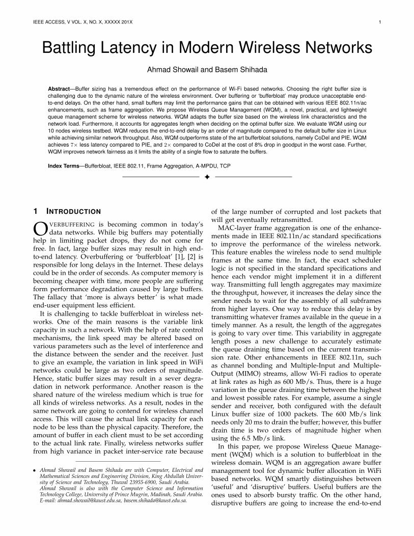
Fig. 1: TCP congestion window, RTT, and egress queueutilization with a one-hop TCP flow in our testbed with6.5 Mb/s link rate. Buffer size correspond to values inthe stock Linux kernel.

3 MOTIVATION

In this section, we motivate the idea of adaptive buffersizing using testbed experimental analysis. We first anal-yse the performance of the default buffering scheme inLinux. After that, we discuss why static buffering is nota feasible option for WiFi networks. Finally, we show theeffect of frame aggregation on the buffer sizing problem.

3.1 How bad is the latency in today’s networks?To highlight the impact of large buffers on networkperformance, we transfer a large file between two wire-less hosts in our testbed while fixing the wireless linkcapacity. Using static link rates help in understandingthe effect of various link rates on network dynamics.Our testbed uses Atheros IEEE 802.11n wireless cards onLinux machines with ath9k [7] drivers. By default, thesize of Linux transmit queue, txqueue, on recent Linuxkernels is 1000 packets. We use a radio channel that doesnot interfere with our campus production network. Thedetailed experimental setup is listed in Section 5. Fig. 1shows the sender TCP congestion window, RTT, andegress buffer occupancy using the 6.5 Mb/s link rate.As window scaling is enabled by default in our testbed,TCP congestion window reaches the limit of 1.6 millionbytes before experiencing a packet loss. We observethat this single file transfer is able to saturate such alarge buffer which results in long queueing delays, withRTT values exceeding 2 seconds. It is worth noting thatqueue occupancy never drops to zero although the TCPcongestion control algorithm (CUBIC by default) halvesthe congestion window in reaction to buffer over flowmultiple times during the experiment. This is a clear ex-ample of bad buffers that does not increase the networkutilization and only contributes to network latency.

3.2 How does frame aggregation affect the buffersizing decision?A-MPDU aggregation logic is not specified in the stan-dard and is implementation dependant. In fact, there is a

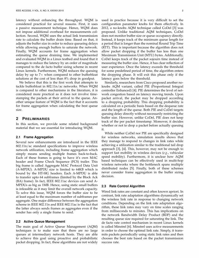
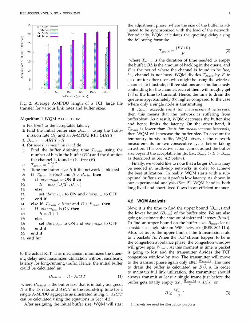
trade-off between using the channel resources effecientlyand lowering the latency. By using large aggregationframes whenever the quality of the channel is good, wecan maximize the channel utilization. On the other hand,one way to minimize the queueing delays is processpackets whenever they are ready. A very basic packetscheduler will wait for a full length A-MPDU frame tobe assembled before trasnmitting it which can potentiallylead to a very high throughput, but will deteriorate thedelay performance. When digging deep in the devicedriver code, we find that the ath9k [7] scheduler aggre-gates as many MPDUs as available at that time in thebuffer subject to the regulatory and receiver constraintsinstead of waiting to assemble maximal allowable A-MPDU aggregates which may maximize throughput.To understand the relation between buffer sizing andthe level of frame aggregation, we repeat the previousTCP file transfer experiment at multiple link rates andtxqueue buffer sizes. We report the mean aggregatelength for various buffer sizes and link rates in Fig. 2.It is clear from this figure that bigger buffers allowthe formation of longer aggregates especially with fastlinks. This is another evidence that fixing the buffer sizeto a small value is not always the best thing to doin order to reduce latency. This figure also shows thatthe link rate directly determines the level of A-MPDUaggregation. Error bars in the figure, which representmaximum and minimum aggregate length, show that theaggregate length varies even with fixed link rates. Theonly exception is with the 6.5 Mb/s link as transmittingmore than one subframe per A-MPDU using the 6.5Mb/s link is not feasible due to the violation of the 4ms regulatory frame transmission requirement in the 5GHz band used in our experiments.

4 APPROACH

In this section, we describe WQM operation and showhow we select various WQM parameters.

4.1 WQM OperationWQM algorithm is described in Algorithm. 1. Clearly,WQM operation pass through two stages. The first stageis called the initial stage and the second stage is calledthe adjustment stage. WQM is going to calculate theinitial buffer size In the initial stage based on a variationof the buffer sizing rule of tuhmb (BDP [8]). In BDP,the buffer should be at least equal to the product ofthe bandwidth of the bottleneck link with the roundtrip delay. However, this rule was initially designed forwired networks, and cannot be used directly in Wi-Fibased networks as it does not account for A-MPDUframe aggregation. For example, it is obvious that thetransmission time, and hence RTT, for a single frame isless than that of a single A-MPDU. In fact, obtaining theend-to-end delay is not always straight forward. This iswhy WQM uses only the single-hop RTT to initialize thebuffer. Then, it starts adapting the buffer size according

IEEE ACCESS, V VOL. X, NO. X, XXXXX 201X 4

Fig. 2: Average A-MPDU length of a TCP large filetransfer for various link rates and buffer sizes.

Algorithm 1 WQM ALGORITHM

1: Fix limit to the acceptable latency2: Find the initial buffer size Binitial using the Trans-

mission rate (R) and an A-MPDU RTT (ARTT ):3: Binitial = ARTT ∗R4: for measurement interval do5: Find the buffer draining time Tdrain using the

number of bits in the buffer (BL) and the durationthe channel is found to be free (F )

6: Tdrain = BL/RF

7: Tune the buffer size B if the network is bloated8: if Tdrain > limit and B > Bmin then9: if alarmhigh is ON then

10: B = max(dB/2e , Bmin)11: else12: set alarmhigh to ON and alarmlow to OFF13: end if14: else if Tdrain < limit and B < Bmax then15: if alarmlow is ON then16: B = B + 117: else18: set alarmlow to ON and alarmhigh to OFF19: end if20: end if21: end for

to the actual RTT. This mechanism minimizes the queu-ing delay and maximizes utilization without sacrificinglatency for long-running traffic. Hence, the initial buffercould be calculated as:

Binitial = R ∗ARTT (1)

where Binitial is the buffer size that is initially assigned,R is the Tx rate, and ARTT is the round-trip time for asingle A-MPDU aggregate as illustrated in Fig. 3. ARTTcan be calculated using the equations in Sect. 4.2.

After assigning the initial buffer size, WQM will start

the adjustment phase, where the size of the buffer is ad-justed to be synchronized with the load of the network.Periodically, WQM calculates the queuing delay usingthe following formula:

Tdrain =(BL/R)

F(2)

where Tdrain is the duration of time needed to emptythe buffer, BL is the amount of backlog in the queue, andF is the period where the channel is found to be free,i.e., channel is not busy. WQM divides Tdrain by F toaccount for other users who might be using the wirelesschannel. To illustrate, if three stations are simultaneouslycontending for the channel, each of them will roughly get1/3 of the time to transmit. Hence, the time to drain thequeue is approximately 3× higher compared to the casewhere only a single node is transmitting.

If Tdrain exceeds limit for measurement intervals,then this means that the network is suffering frombufferbloat. As a result, WQM decreases the buffer sizeand hence limits the latency. On the other hand, ifTdrain is lower than limit for measurement intervals,then WQM will increase the buffer size. To account fortemporary bursty traffic, WQM observes the networkmeasurements for two consecutive cycles before takingan action. This corrective action cannot adjust the buffersize beyond the acceptable limits, (i.e., Bmax > B > Bminas described in Sec. 4.2 below).

Finally, we would like to note that a larger Binitial maybe needed in multi-hop networks in order to achievethe best utilization . In reality, WQM starts with a sub-optimal buffer size as it prefers low latency. As shown inour experimental analysis (Sec. 5), WQM handles bothlong-lived and short-lived flows in an efficient manner.

4.2 WQM Analysis

Now, it is the time to find the upper bound (Bmax) andthe lower bound (Bmin) of the buffer size. We are alsogoing to estimate the amount of tolerated latency (limit).To find an upper bound on the buffer size, Bmax, let usconsider a single stream WiFi network (IEEE 802.11n).Also, let us fix the upper limit of the transmission rateto λ packets1/s. When the TCP stream happen to be inthe congestion avoidance phase, the congestion windowwill grow upto Wmax. At this moment in time, a packetis going to lost and the transmitter divides the TCPcongestion window by two. The transmitter will moveto the transmit phase again only after Wmax/2

λ . The timeto drain the buffer is calculated as B/λ s. In orderto maintain full link utilization, the transmitter shouldalways transmit at least a single frame just before thebuffer gets totally empty (i.e., Wmax/2

λ ≤ B/λ), or

B ≥ Wmax

2(3)

1. Packets are used for illustration purposes.

IEEE ACCESS, V VOL. X, NO. X, XXXXX 201X 5

Parameter ValueTslot slot duration = 9 µsTSIFS shortest inter-frame space = 16 µsTDIFS distributed inter-frame space = 34 µsTPHY physical layer duration = 33 µsCWmin minimum size of contention window = 15CWmax maximum size of contention window = 1023TBO average back-off interval = (CWmin−1)∗Tslot/2R physical rate (Mb/s)Rbasic basic physical rate = 6 Mb/sK maximum A-MPDU sizeTMAC MAC header duration = LMAC/RLMAC MAC overhead = 38 B = 304 bTDATA data frame duration = LDATA/RLDATA data frame size = 1500 B = 12000 bTTCP−ACK TCP ACK duration = LTCP−ACK/RLTCP−ACK TCP ACK size = 40 B = 320 bTBACK block ACK frame duration = LBACK/Rbasic

LBACK block ACK frame size = 30 B = 240 b

TABLE 1: System parameters of WiFi Network (IEEE802.11n) [9].

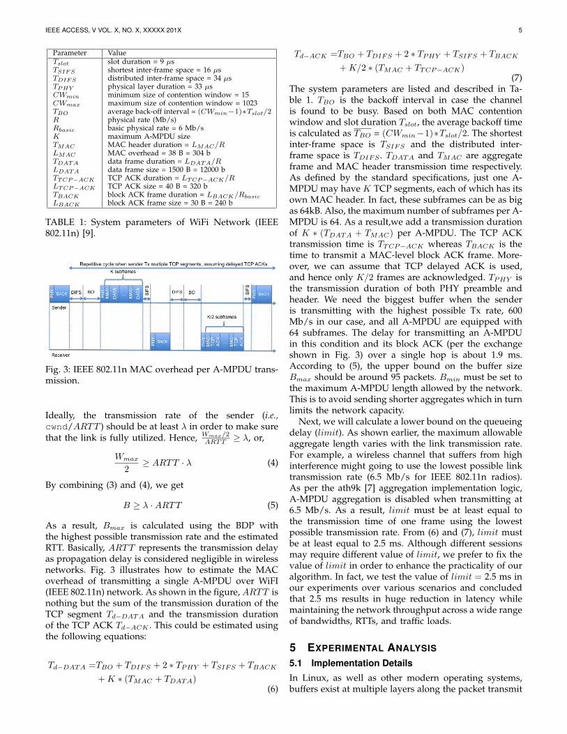
Fig. 3: IEEE 802.11n MAC overhead per A-MPDU trans-mission.

Ideally, the transmission rate of the sender (i.e.,cwnd/ARTT ) should be at least λ in order to make surethat the link is fully utilized. Hence, Wmax/2

ARTT ≥ λ, or,

Wmax

2≥ ARTT · λ (4)

By combining (3) and (4), we get

B ≥ λ ·ARTT (5)

As a result, Bmax is calculated using the BDP withthe highest possible transmission rate and the estimatedRTT. Basically, ARTT represents the transmission delayas propagation delay is considered negligible in wirelessnetworks. Fig. 3 illustrates how to estimate the MACoverhead of transmitting a single A-MPDU over WiFI(IEEE 802.11n) network. As shown in the figure, ARTT isnothing but the sum of the transmission duration of theTCP segment Td−DATA and the transmission durationof the TCP ACK Td−ACK . This could be estimated usingthe following equations:

Td−DATA =TBO + TDIFS + 2 ∗ TPHY + TSIFS + TBACK

+K ∗ (TMAC + TDATA)(6)

Td−ACK =TBO + TDIFS + 2 ∗ TPHY + TSIFS + TBACK

+K/2 ∗ (TMAC + TTCP−ACK)(7)

The system parameters are listed and described in Ta-ble 1. TBO is the backoff interval in case the channelis found to be busy. Based on both MAC contentionwindow and slot duration Tslot, the average backoff timeis calculated as TBO = (CWmin−1)∗Tslot/2. The shortestinter-frame space is TSIFS and the distributed inter-frame space is TDIFS . TDATA and TMAC are aggregateframe and MAC header transmission time respectively.As defined by the standard specifications, just one A-MPDU may have K TCP segments, each of which has itsown MAC header. In fact, these subframes can be as bigas 64kB. Also, the maximum number of subframes per A-MPDU is 64. As a result,we add a transmission durationof K ∗ (TDATA + TMAC) per A-MPDU. The TCP ACKtransmission time is TTCP−ACK whereas TBACK is thetime to transmit a MAC-level block ACK frame. More-over, we can assume that TCP delayed ACK is used,and hence only K/2 frames are acknowledged. TPHY isthe transmission duration of both PHY preamble andheader. We need the biggest buffer when the senderis transmitting with the highest possible Tx rate, 600Mb/s in our case, and all A-MPDU are equipped with64 subframes. The delay for transmitting an A-MPDUin this condition and its block ACK (per the exchangeshown in Fig. 3) over a single hop is about 1.9 ms.According to (5), the upper bound on the buffer sizeBmax should be around 95 packets. Bmin must be set tothe maximum A-MPDU length allowed by the network.This is to avoid sending shorter aggregates which in turnlimits the network capacity.

Next, we will calculate a lower bound on the queueingdelay (limit). As shown earlier, the maximum allowableaggregate length varies with the link transmission rate.For example, a wireless channel that suffers from highinterference might going to use the lowest possible linktransmission rate (6.5 Mb/s for IEEE 802.11n radios).As per the ath9k [7] aggregation implementation logic,A-MPDU aggregation is disabled when transmitting at6.5 Mb/s. As a result, limit must be at least equal tothe transmission time of one frame using the lowestpossible transmission rate. From (6) and (7), limit mustbe at least equal to 2.5 ms. Although different sessionsmay require different value of limit, we prefer to fix thevalue of limit in order to enhance the practicality of ouralgorithm. In fact, we test the value of limit = 2.5 ms inour experiments over various scenarios and concludedthat 2.5 ms results in huge reduction in latency whilemaintaining the network throughput across a wide rangeof bandwidths, RTTs, and traffic loads.

5 EXPERIMENTAL ANALYSIS

5.1 Implementation Details

In Linux, as well as other modern operating systems,buffers exist at multiple layers along the packet transmit

IEEE ACCESS, V VOL. X, NO. X, XXXXX 201X 6

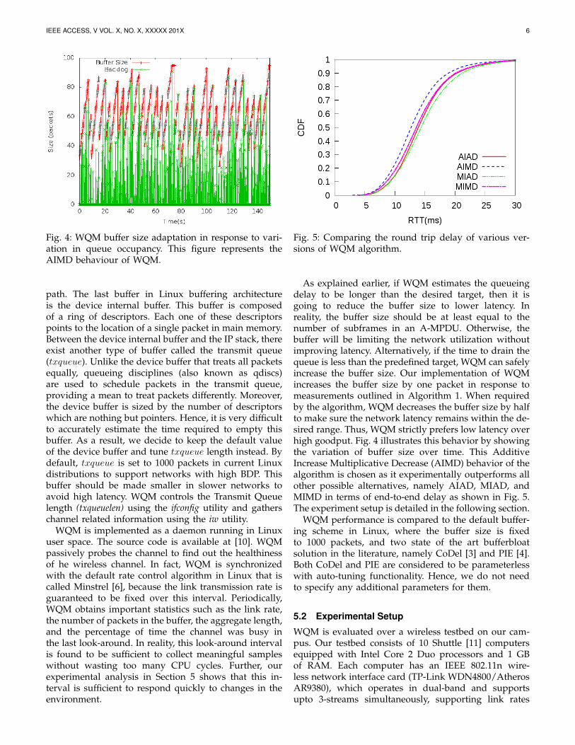
Fig. 4: WQM buffer size adaptation in response to vari-ation in queue occupancy. This figure represents theAIMD behaviour of WQM.

path. The last buffer in Linux buffering architectureis the device internal buffer. This buffer is composedof a ring of descriptors. Each one of these descriptorspoints to the location of a single packet in main memory.Between the device internal buffer and the IP stack, thereexist another type of buffer called the transmit queue(txqueue). Unlike the device buffer that treats all packetsequally, queueing disciplines (also known as qdiscs)are used to schedule packets in the transmit queue,providing a mean to treat packets differently. Moreover,the device buffer is sized by the number of descriptorswhich are nothing but pointers. Hence, it is very difficultto accurately estimate the time required to empty thisbuffer. As a result, we decide to keep the default valueof the device buffer and tune txqueue length instead. Bydefault, txqueue is set to 1000 packets in current Linuxdistributions to support networks with high BDP. Thisbuffer should be made smaller in slower networks toavoid high latency. WQM controls the Transmit Queuelength (txqueuelen) using the ifconfig utility and gatherschannel related information using the iw utility.

WQM is implemented as a daemon running in Linuxuser space. The source code is available at [10]. WQMpassively probes the channel to find out the healthinessof he wireless channel. In fact, WQM is synchronizedwith the default rate control algorithm in Linux that iscalled Minstrel [6], because the link transmission rate isguaranteed to be fixed over this interval. Periodically,WQM obtains important statistics such as the link rate,the number of packets in the buffer, the aggregate length,and the percentage of time the channel was busy inthe last look-around. In reality, this look-around intervalis found to be sufficient to collect meaningful sampleswithout wasting too many CPU cycles. Further, ourexperimental analysis in Section 5 shows that this in-terval is sufficient to respond quickly to changes in theenvironment.

Fig. 5: Comparing the round trip delay of various ver-sions of WQM algorithm.

As explained earlier, if WQM estimates the queueingdelay to be longer than the desired target, then it isgoing to reduce the buffer size to lower latency. Inreality, the buffer size should be at least equal to thenumber of subframes in an A-MPDU. Otherwise, thebuffer will be limiting the network utilization withoutimproving latency. Alternatively, if the time to drain thequeue is less than the predefined target, WQM can safelyincrease the buffer size. Our implementation of WQMincreases the buffer size by one packet in response tomeasurements outlined in Algorithm 1. When requiredby the algorithm, WQM decreases the buffer size by halfto make sure the network latency remains within the de-sired range. Thus, WQM strictly prefers low latency overhigh goodput. Fig. 4 illustrates this behavior by showingthe variation of buffer size over time. This AdditiveIncrease Multiplicative Decrease (AIMD) behavior of thealgorithm is chosen as it experimentally outperforms allother possible alternatives, namely AIAD, MIAD, andMIMD in terms of end-to-end delay as shown in Fig. 5.The experiment setup is detailed in the following section.

WQM performance is compared to the default buffer-ing scheme in Linux, where the buffer size is fixedto 1000 packets, and two state of the art bufferbloatsolution in the literature, namely CoDel [3] and PIE [4].Both CoDel and PIE are considered to be parameterlesswith auto-tuning functionality. Hence, we do not needto specify any additional parameters for them.

5.2 Experimental Setup

WQM is evaluated over a wireless testbed on our cam-pus. Our testbed consists of 10 Shuttle [11] computersequipped with Intel Core 2 Duo processors and 1 GBof RAM. Each computer has an IEEE 802.11n wire-less network interface card (TP-Link WDN4800/AtherosAR9380), which operates in dual-band and supportsupto 3-streams simultaneously, supporting link rates

IEEE ACCESS, V VOL. X, NO. X, XXXXX 201X 7

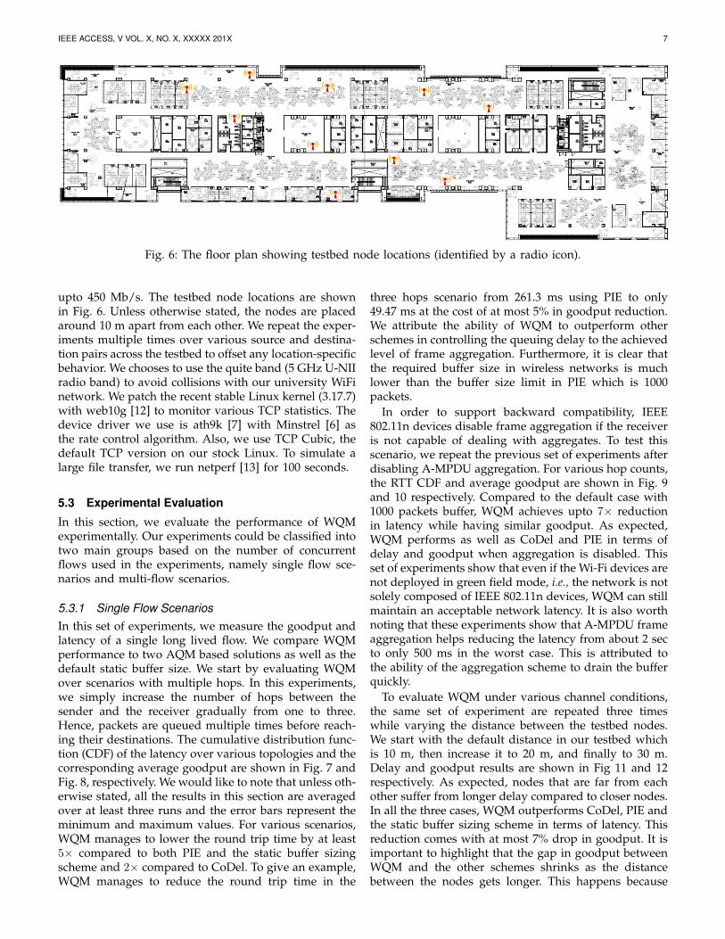
Fig. 6: The floor plan showing testbed node locations (identified by a radio icon).

upto 450 Mb/s. The testbed node locations are shownin Fig. 6. Unless otherwise stated, the nodes are placedaround 10 m apart from each other. We repeat the exper-iments multiple times over various source and destina-tion pairs across the testbed to offset any location-specificbehavior. We chooses to use the quite band (5 GHz U-NIIradio band) to avoid collisions with our university WiFinetwork. We patch the recent stable Linux kernel (3.17.7)with web10g [12] to monitor various TCP statistics. Thedevice driver we use is ath9k [7] with Minstrel [6] asthe rate control algorithm. Also, we use TCP Cubic, thedefault TCP version on our stock Linux. To simulate alarge file transfer, we run netperf [13] for 100 seconds.

5.3 Experimental Evaluation

In this section, we evaluate the performance of WQMexperimentally. Our experiments could be classified intotwo main groups based on the number of concurrentflows used in the experiments, namely single flow sce-narios and multi-flow scenarios.

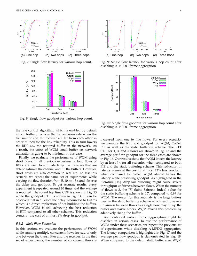
5.3.1 Single Flow ScenariosIn this set of experiments, we measure the goodput andlatency of a single long lived flow. We compare WQMperformance to two AQM based solutions as well as thedefault static buffer size. We start by evaluating WQMover scenarios with multiple hops. In this experiments,we simply increase the number of hops between thesender and the receiver gradually from one to three.Hence, packets are queued multiple times before reach-ing their destinations. The cumulative distribution func-tion (CDF) of the latency over various topologies and thecorresponding average goodput are shown in Fig. 7 andFig. 8, respectively. We would like to note that unless oth-erwise stated, all the results in this section are averagedover at least three runs and the error bars represent theminimum and maximum values. For various scenarios,WQM manages to lower the round trip time by at least5× compared to both PIE and the static buffer sizingscheme and 2× compared to CoDel. To give an example,WQM manages to reduce the round trip time in the

three hops scenario from 261.3 ms using PIE to only49.47 ms at the cost of at most 5% in goodput reduction.We attribute the ability of WQM to outperform otherschemes in controlling the queuing delay to the achievedlevel of frame aggregation. Furthermore, it is clear thatthe required buffer size in wireless networks is muchlower than the buffer size limit in PIE which is 1000packets.

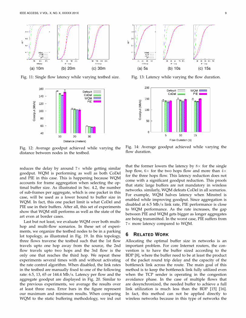
In order to support backward compatibility, IEEE802.11n devices disable frame aggregation if the receiveris not capable of dealing with aggregates. To test thisscenario, we repeat the previous set of experiments afterdisabling A-MPDU aggregation. For various hop counts,the RTT CDF and average goodput are shown in Fig. 9and 10 respectively. Compared to the default case with1000 packets buffer, WQM achieves upto 7× reductionin latency while having similar goodput. As expected,WQM performs as well as CoDel and PIE in terms ofdelay and goodput when aggregation is disabled. Thisset of experiments show that even if the Wi-Fi devices arenot deployed in green field mode, i.e., the network is notsolely composed of IEEE 802.11n devices, WQM can stillmaintain an acceptable network latency. It is also worthnoting that these experiments show that A-MPDU frameaggregation helps reducing the latency from about 2 secto only 500 ms in the worst case. This is attributed tothe ability of the aggregation scheme to drain the bufferquickly.

To evaluate WQM under various channel conditions,the same set of experiment are repeated three timeswhile varying the distance between the testbed nodes.We start with the default distance in our testbed whichis 10 m, then increase it to 20 m, and finally to 30 m.Delay and goodput results are shown in Fig 11 and 12respectively. As expected, nodes that are far from eachother suffer from longer delay compared to closer nodes.In all the three cases, WQM outperforms CoDel, PIE andthe static buffer sizing scheme in terms of latency. Thisreduction comes with at most 7% drop in goodput. It isimportant to highlight that the gap in goodput betweenWQM and the other schemes shrinks as the distancebetween the nodes gets longer. This happens because

IEEE ACCESS, V VOL. X, NO. X, XXXXX 201X 8

(a) One hop (b) Two hops (c) Three hops

Fig. 7: Single flow latency for various hop count.

Fig. 8: Single flow goodput for various hop count.

the rate control algorithm, which is enabled by defaultin our testbed, reduces the transmission rate when thetransmitter and the receiver are far from each other inorder to increase the link reliability. This in turn lowersthe BDP i.e., the required buffer in the network. Asa result, the effect of WQM small buffer on networkutilization is going to be minimal in this case.

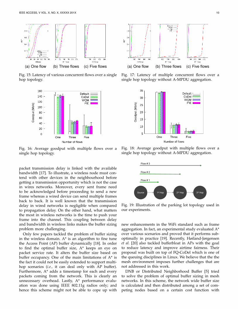
Finally, we evaluate the performance of WQM usingshort flows. In all previous experiments, long flows of100 s are used to simulate large file transfers that areable to saturate the channel and fill the buffers. However,short flows are also common in real life. To test thisscenario we repeat the same set of experiments whilevarying the flow duration from 5, 10, to 15 s and observethe delay and goodput. To get accurate results, everyexperiment is repeated around 10 times and the averageis reported. The round trip time CDF is shown in Fig. 13while the goodput CDF is shown in Fig. 14. It can beobserved that in all cases the delay is bounded to 150 mswhich is a direct implication of not building the buffers.However, WQM is still achieving the best reductionin RTT compared to all other schemes. This reductioncomes at the cost of at most 8% drop in goodput.

5.3.2 Multi Flow ScenariosIn this section, we evaluate the performance of WQMwhile running multiple concurrent flows instead of onlyone between the transmitter and the receiver. In the firstset of experiments, the number of concurrent flows is

(a) One hop (b) Two hops (c) Three hops

Fig. 9: Single flow latency for various hop count afterdisabling A-MPDU frame aggregation.

Fig. 10: Single flow goodput for various hop count afterdisabling A-MPDU frame aggregation.

increased from one to five flows. For every scenario,we measure the RTT and goodput for WQM, CoDel,PIE as well as the static buffering scheme. The RTTCDF for 1, 3, and 5 flows are shown in Fig. 15 and theaverage per flow goodput for the three cases are shownin Fig. 16. Our results show that WQM lowers the latencyby at least 5× for all scenarios when compared to bothPIE and the static buffering scheme. This reduction inlatency comes at the cost of at most 13% less goodput.when compared to CoDel, WQM almost halves thelatency while preserving goodput. As highlighted in theliterature [14], drop-tail buffering might cause severethroughput unfairness between flows. When the numberof flows is 3, the JFI (Jains Fairness Index) value forthe static buffering scheme is 0.7, compared to 0.99 forWQM. The reason for this anomaly is the large buffersused in the static buffering scheme which lead to severeunfairness between flows as a single flow may fill up thebuffer and starve others. WQM avoids this problem byadaptively sizing the buffer .

As mentioned earlier, frame aggregation might bedisabled in certain cases. To test the performance ofWQM under these scenarios, we repeat the previous setof experiments while disabling A-MPDU aggregation.The latency comparison is highlighted in Fig. 17 and theaverage per flow goodput is demonstrated in Fig. 18.When compared to the default static buffer size, WQM

IEEE ACCESS, V VOL. X, NO. X, XXXXX 201X 9

(a) 10m (b) 20m (c) 30m

Fig. 11: Single flow latency while varying testbed size.

Fig. 12: Average goodput achieved while varying thedistance between nodes in the testbed.

reduces the delay by around 7× while getting similargoodput. WQM is performing as well as both CoDeland PIE in this case. This is happening because WQMaccounts for frame aggregation when selecting the op-timal buffer size. As illustrated in Sec. 4.2, the numberof sub-frames per aggregate, which is one packet in thiscase, will be used as a lower bound to buffer size inWQM. In fact, this one packet limit is what CoDel andPIE use in their buffers. After all, this set of experimentsshow that WQM still performs as well as the state of theart even at border cases.

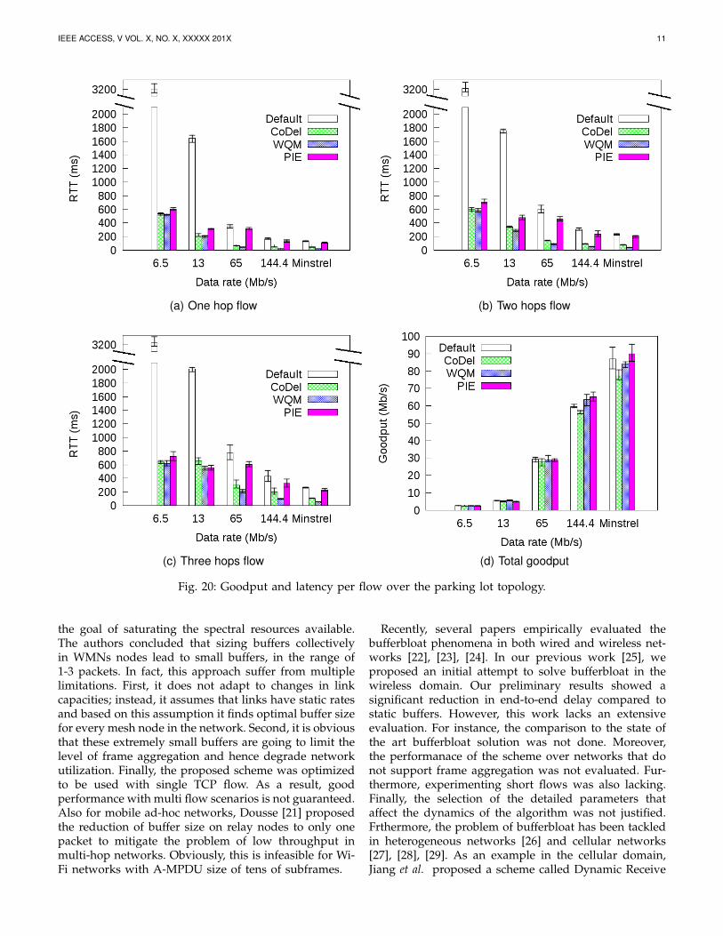
Last but not least, we evaluate WQM over both multi-hop and multi-flow scenarios. In these set of experi-ments, we organize the testbed nodes to be in a parkinglot topology, as illustrated in Fig. 19. In this topology,three flows traverse the testbed such that the 1st flowtravels upto one hop away from the source, the 2ndflow travels upto two hops and the 3rd flow is theonly one that reaches the third hop. We repeat theseexperiments several times with and without activatingthe rate control algorithm. When disabled, the link ratesin the testbed are manually fixed to one of the followingrate: 6.5, 13, 65 or 144.4 Mb/s. Latency per flow and theaggregate goodput are displayed in Fig. 20. Similar tothe previous experiments, we average the results overat least three runs. Error bars in the figure representour maximum and minimum results. When comparingWQM to the static buffering methodology, we ind out

(a) 5s (b) 10s (c) 15s

Fig. 13: Latency while varying the flow duration.

Fig. 14: Average goodput achieved while varying theflow duration.

that the former lowers the latency by 8× for the singlehop flow, 6× for the two hops flow and more than 4×for the three hops flow. This latency reduction does notcome with a significant goodput reduction. This proofsthat static large buffers are not mandatory in wirelessnetworks. similarly, WQM defeats CoDel in all scenarios.For example, WQM halves latency when Minstrel isenabled while improving goodput. Since aggregation isdisabled at 6.5 Mb/s link rate, PIE performance is closeto WQM performance. As the rate increases, the gapbetween PIE and WQM gets bigger as longer aggregatesare being transmitted. In the worst case, PIE suffers from7× more latency compared to WQM.

6 RELATED WORK

Allocating the optimal buffer size in networks is animportant problem. For core Internet routers, the con-vention is to have the buffer sized according to theBDP [8], where the buffer need to be at least the productof the packet round trip delay and the capacity of thebottleneck link across the route. The main goal of thismethod is to keep the bottleneck link fully utilized evenwhen the TCP sender is operating in the congestionavoidance phase. In the case of multiple flows thatare desynchronized, the needed buffer to achieve a fulllink utilization is much less than the BDP [15] [16].In fact, this method can not be applied directly towireless networks because in this type of networks the

IEEE ACCESS, V VOL. X, NO. X, XXXXX 201X 10

(a) One flow (b) Three flows (c) Five flows

Fig. 15: Latency of various concurrent flows over a singlehop topology.

Fig. 16: Average goodput with multiple flows over asingle hop topology.

packet transmission delay is linked with the availablebandwidth [17]. To illustrate, a wireless node must con-tend with other devices in the neighbourhood beforegetting a transmission opportunity which is not the casein wires networks. Moreover, every sent frame needto be acknowledged before proceeding to send a newframe whereas a wired device can send multiple framesback to back. It is well known that the transmissiondelay in wired networks is negligible when comparedto propagation delay. On the other hand, what mattersthe most in wireless networks is the time to push yourframe into the channel. This coupling between delayand bandwidth in wireless links makes the buffer sizingproblem more challenging.

Only few papers tackled the problem of buffer sizingin the wireless domain. A* is an algorithm to fine tunethe Access Point (AP) buffer dynamically [18]. In orderto find the optimal buffer size, A* keeps an eye onpacket service rate. It alters the buffer size based onbuffer occupancy. One of the main limitations of A* isthe fact it could not be easily extended to support multi-hop scenarios (i.e., it can deal only with AP buffer).Furthermore, A* adds a timestamp for each and everypackets coming from the network. This is clearly anunnecessary overhead. Lastly, A* performance evalu-ation was done using IEEE 802.11g radios only; andhence this scheme might not be able to cope up with

(a) One flow (b) Three flows (c) Five flows

Fig. 17: Latency of multiple concurrent flows over asingle hop topology without A-MPDU aggregation.

Fig. 18: Average goodput with multiple flows over asingle hop topology without A-MPDU aggregation.

Source 1st Hop 2nd Hop 3rd Hop

Flow # 1

Flow # 2

Flow # 3

Fig. 19: Illustration of the parking lot topology used inour experiments.

new enhancements in the WiFi standard such as frameaggregation. In fact, an experimental study evaluated A*over various scenarios and proved that it performs sub-optimally in practice [19]. Recently, Høiland-Jørgensenet al. [20] also tackled bufferbloat in APs with the goalto reduce latency and improve airtime fairness. Theirproposal was built on top of FQ-CoDel which is one ofthe queuing disciplines in Linux. We believe that the themesh environment imposes further challenges that arenot addressed in this work.

DNB or Distributed Neighborhood Buffer [5] triedto solve the problem of optimal buffer sizing in meshnetworks. In this scheme, the network wide buffer sizeis calculated and then distributed among a set of com-peting nodes based on a certain cost function with

IEEE ACCESS, V VOL. X, NO. X, XXXXX 201X 11

(a) One hop flow (b) Two hops flow

(c) Three hops flow (d) Total goodput

Fig. 20: Goodput and latency per flow over the parking lot topology.

the goal of saturating the spectral resources available.The authors concluded that sizing buffers collectivelyin WMNs nodes lead to small buffers, in the range of1-3 packets. In fact, this approach suffer from multiplelimitations. First, it does not adapt to changes in linkcapacities; instead, it assumes that links have static ratesand based on this assumption it finds optimal buffer sizefor every mesh node in the network. Second, it is obviousthat these extremely small buffers are going to limit thelevel of frame aggregation and hence degrade networkutilization. Finally, the proposed scheme was optimizedto be used with single TCP flow. As a result, goodperformance with multi flow scenarios is not guaranteed.Also for mobile ad-hoc networks, Dousse [21] proposedthe reduction of buffer size on relay nodes to only onepacket to mitigate the problem of low throughput inmulti-hop networks. Obviously, this is infeasible for Wi-Fi networks with A-MPDU size of tens of subframes.

Recently, several papers empirically evaluated thebufferbloat phenomena in both wired and wireless net-works [22], [23], [24]. In our previous work [25], weproposed an initial attempt to solve bufferbloat in thewireless domain. Our preliminary results showed asignificant reduction in end-to-end delay compared tostatic buffers. However, this work lacks an extensiveevaluation. For instance, the comparison to the state ofthe art bufferbloat solution was not done. Moreover,the performanace of the scheme over networks that donot support frame aggregation was not evaluated. Fur-thermore, experimenting short flows was also lacking.Finally, the selection of the detailed parameters thataffect the dynamics of the algorithm was not justified.Frthermore, the problem of bufferbloat has been tackledin heterogeneous networks [26] and cellular networks[27], [28], [29]. As an example in the cellular domain,Jiang et al. proposed a scheme called Dynamic Receive

IEEE ACCESS, V VOL. X, NO. X, XXXXX 201X 12

Window Adjustment (DRWA) [30] that modifies the TCPstack instead of dealing with the buffer size directly.DRWA limits the amount of buffering inside the networkby tuning the size of TCP receive window. Also forcellular networks, Chan et al. proposed a scheme calledSoD or (Sum-of-Delay) [31] that estimates the optimalbuffer size in 3G/4G networks. The main idea is tomodify TCP congestion control to function based onestimated queue length instead of packet loss events.Both of these schemes have practical limitations becauseof the large deployed base of TCP.

Warrier et al. [32] proposed a differential backlogcongestion control for wireless networks. The idea isto throttle the flow control of the sender based on thequeue back pressure. Hence, if the queue grows beyondcertain threshold, the sender will be reducing its transmitrate and vice versa. This is opposite to what WQMdoes. One limitation of such approach is the need ofthe queue occupancy information from several hops inthe multi-hop networks. Transferring this informationover multiple hops is a considerable overhead thatwill affect the practicality of the proposed approach.Alternatively, WQM works with local knowledge evenfor multihop networks. Recently, the authors in [33]proposed a scheme to adaptively change the aggregatesize based on nodes mobility patters. We envision thatsuch scheme would be complementary to WQM.

7 CONCLUSIONRecent enhancements in IEEE 802.11n/ac standard spec-ifications, such as A-MPDU frame aggregation, make itmore difficult to find the optimal buffer size in WiFibased networks. Large buffers may lead to long end-to-end delays in the order of seconds. We are proposinga novel, practical, and dynamic buffer management toolcalled WQM. It selects the optimal buffer size based onseveral parameters such as network congestion, channelinterference intensity, and the level of frame aggregation.WQM is evaluated using a 10 nodes wireless testbed.We prove through experiments over various single-hopand multi-hop scenarios that WQM is able to cut downthe queuing delay by a factor of 8× when comparedto static buffer sizing. Further, WQM outperforms otherstate of the art bufferbloat solutions such as CoDel andPIE by a factor of 7× in terms of delay reduction. In theworst case, this reduction comes at the cost of 8% dropin goodput. Finally, we show that WQM improves flowfairness by preventing a single flow from saturating thebuffers.

As future work, we are looking into several new chal-lenges. One of them is to evaluate WQM over varioustypes of flows across different topologies. Furthermore,we would like to assess WQM using selective dropmechanisms. Also, it is interesting to evaluate how doesTCP pacing interacts with frame aggregation in wirelessnetworks. Moreover, we would like to understand theconsequences of introducing an adaptive look-around in-terval to WQM. Finally, we would also like to test WQM

using wireless devices with IEEE 802.11ac compatibleradios.

REFERENCES

[1] J. Gettys and K. Nichols, “Bufferbloat: dark buffers in the inter-net,” Commun. ACM, January 2012.

[2] C. Staff, “Bufferbloat: what’s wrong with the internet?” Commun.ACM, vol. 55, no. 2, Feb. 2012.

[3] K. Nichols and V. Jacobson, “Controlling queue delay,” Queue,vol. 10, no. 5, May 2012.

[4] R. Pan, P. Natarajan, F. Baker, and G. White, “Proportional inte-gral controller enhanced (PIE): A lightweight control scheme toaddress the bufferbloat problem,” Tech. Rep., 2017.

[5] K. Jamshaid, B. Shihada, A. Showail, and P. Levis, “Deflating linkbuffers in a wireless mesh network,” Ad Hoc Networks, vol. 16,no. 0, 2014.

[6] D. Smithies and F. Fietkau, Minstrel Rate Control Algorithm.[Online]. Available: http://wireless.kernel.org/en/developers/Documentation/mac80211/RateControl/minstrel

[7] Ath9k FOSS drivers. http://wireless.kernel.org/en/users/Drivers/ath9k.

[8] C. Villamizar and C. Song, “High performance TCP in ANSNET,”SIGCOMM Comput. Commun. Rev., vol. 24, no. 5, pp. 45–60, Oct.1994.

[9] IEEE LAN/MAN Standards Committee, IEEE 802.11 Wireless LANmedium access control (MAC) and physical layer (PHY) specifications,IEEE, 2012.

[10] WQM source code. http://www.shihada.com/download.php?file=wqm.zip.

[11] Shuttle Inc. http://www.shuttle.com.[12] The Web10g Project. http://www.web10g.org/.[13] Netperf. http://www.netperf.org/netperf/.[14] S. R. Pokhrel, M. Panda, and H. L. Vu, “Analytical modeling of

multipath tcp over last-mile wireless,” IEEE/ACM Trans. Netw.,vol. 25, no. 3, Jun. 2017.

[15] G. Appenzeller, I. Keslassy, and N. McKeown, “Sizing routerbuffers,” in Proceedings of the 2004 conference on Applications,technologies, architectures, and protocols for computer communications,ser. SIGCOMM ’04, 2004.

[16] M. Enachescu, Y. Ganjali, A. Goel, N. McKeown, and T. Rough-garden, “Routers with very small buffers,” in Proc. of the IEEEINFOCOM ’06, Apr. 2006.

[17] K. Chen, Y. Xue, S. Shah, and K. Nahrstedt, “Understandingbandwidth-delay product in mobile ad hoc networks,” ElsevierComputer Communications, vol. 27, no. 10, June 2004.

[18] T. Li, D. Leith, and D. Malone, “Buffer sizing for 802.11-basednetworks,” IEEE/ACM Transactions on Networking, 2011.

[19] D. Taht, “What I think is wrong with eBDP in debloat-testing,” https://lists.bufferbloat.net/pipermail/bloat-devel/2011-November/000280.html.

[20] T. Høiland-Jørgensen, M. Kazior, D. Taht, P. Hurtig, and A. Brun-strom, “Ending the anomaly: Achieving low latency and airtimefairness in WiFi,” in 2017 USENIX Annual Technical Conference(USENIX ATC 17), Santa Clara, CA, 2017.

[21] O. Dousse, “Revising buffering in CSMA/CA wireless multihopnetworks,” in Proc. of the IEEE SECON ’07, Jun. 2007.

[22] M. Allman, “Comments on bufferbloat,” SIGCOMM Comput. Com-mun. Rev., vol. 43, no. 1, Jan. 2012.

[23] A. Showail, K. Jamshaid, and B. Shihada, “An empirical evalua-tion of bufferbloat in IEEE 802.11n wireless networks,” in WirelessCommunications and Networking Conference (WCNC), IEEE, April2014.

[24] O. Hohlfeld, E. Pujol, F. Ciucu, A. Feldmann, and P. Barford, “AQoE perspective on sizing network buffers,” in Proceedings of the2014 Conference on Internet Measurement Conference, ser. IMC ’14,2014.

[25] A. Showail, K. Jamshaid, and B. Shihada, “WQM: An aggregation-aware queue management scheme for IEEE 802.11n based net-works,” in Proceedings of the 2014 ACM SIGCOMM Workshop onCapacity Sharing Workshop, ser. CSWS ’14, 2014.

[26] B. Felix, A. Santos, B. Kantarci, and M. Nogueira, “CD-ASM:A new queuing paradigm to overcome bufferbloat effects inhetnets,” in 2017 IEEE 28th Annual International Symposium onPersonal, Indoor, and Mobile Radio Communications (PIMRC), 2017.

IEEE ACCESS, V VOL. X, NO. X, XXXXX 201X 13

[27] Y. Guo, F. Qian, Q. A. Chen, Z. M. Mao, and S. Sen, “Understand-ing on-device bufferbloat for cellular upload,” in Proceedings of the2016 ACM on Internet Measurement Conference. ACM, 2016.

[28] X. Liu, F. Ren, R. Shu, T. Zhang, and T. Dai, “Mitigatingbufferbloat with receiver-based TCP flow control mechanismin cellular networks,” Advances in Computer Communications andNetworks: From Green, Mobile, Pervasive Networking to Big DataComputing, p. 65, 2016.

[29] J. D. Beshay, A. T. Nasrabadi, R. Prakash, and A. Francini, “Onactive queue management in cellular networks,” in 2017 IEEEConference on Computer Communications Workshops (INFOCOMWKSHPS), 2017.

[30] H. Jiang, Y. Wang, K. Lee, and I. Rhee, “DRWA: a receiver-centricsolution to bufferbloat in cellular networks,” IEEE Transactions onMobile Computing, vol. 15, no. 11, 2016.

[31] S. Chan, K. Chan, K. Liu, and J. Lee, “On queue length and linkbuffer size estimation in 3G/4G mobile data networks,” MobileComputing, IEEE Transactions on, vol. 13, no. 6, June 2014.

[32] A. Warrier, S. Janakiraman, S. Ha, and I. Rhee, “DiffQ: Practicaldifferential backlog congestion control for wireless networks,” inINFOCOM 2009, IEEE, 2009.

[33] S. Byeon, K. Yoon, O. Lee, S. Choi, W. Cho, and S. Oh, “MoFA:Mobility-aware frame aggregation in Wi-Fi,” in Proceedings of theTenth ACM Conference on Emerging Networking Experiments andTechnologies, ser. CoNEXT ’14, 2014.