IEEE CO~TROL, VOL. NO. Optimal Large-Scale Power

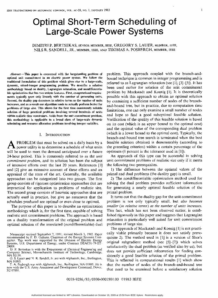
IEEE TRANSACTIONS ON AUTOMATIC CO~TROL, VOL. AC-28, NO. 1: JANUARY 1983 I

Optimal Short-Term Scheduling of Large-Scale Power Systems

Abstruct--This paper is concerned with the longstanding problem of optimal unit commitment in an electric power system. We follow the traditional formulation of this problem which gives rise to a large-scale, dynamic, mixed-integer programming problem. We describe a solution methodology based on duality, Lagrangian relaxation and nondifferentiable optimization that has two unique features. First, computational requirements typically grow only linearly witb the number of generating units. Second, the duality gap decreases in relative terms as the number of units increases, and as a result our algorithm tends to actually perform better for problems of large size. This allows for the first time consistently reliable solution of large practical problems involving several hundreds of units within realistic time constraints. Aside from the unit commilment problem. this methodology is applicable to a broad class of large-scale dpamic scheduling and resource allocation problems involving integer variables.

A I. INTRODUCTION

PROBLEM that must be solved on a daily basis by a power utility is to determine a schedule of what units

will be used to meet the demand anticipated over a future 24-hour period. This is commonly referred to as the unit Commitment problem, and its solution has been the subject of intensive efforts over the last 20 years. References [l] and [2] give an extensive account of these efforts and an appraisal of the state of the art. Generally, the available approaches can be categorized into two groups. The first group consists of rigorous optimization approaches that are impractical for application to problems of realistic size. The second group consists of heuristic approaches that are actually used in practice, but give no assurance that the schedules produced are optimal or even close to optimal.

The purpose of this paper is to describe an optimization methodology which is, for the first time, capable of solving realistic unit commitment problems. The approach is based on a duality transformation of the original problem and optimal solution of the associated (nondifferentiable) dual

recommended by F. D. Galiana. Chairman of the Energy Systems Com- Manuscript received September 7. 1981 : revised March 3. 1982. Paper

mittee. This work was supported by the Division of Electric Energy Systems. U.S. Department of Energy. under Contract DEACOI-79-ET- 29008.

D. P. Bertsekas is with the Department of Electrical Engineering and Computer Science, Massachusetts Institute of Technology, Cambridge. MA 02139.

MA 01803. G. S. Lauer and N. R. Sandell, Jr. are with Alphatech. Inc., Burlington,

now with the U.S. Army Armament and Development Command, Dover, T. A. Posbergh was with Alphatech. Inc.. Burlington. MA 01803. He is

NJ 07801.

problem. This approach coupled with the branch-and- bound technique is common in integer programming and is referred to as Lagrangian relaxation (see [l], [3]-[5]). It has been used earlier for solution of the unit commitment problem by Muckstadt and Koenig [l]. It is theoretically possible with this approach to obtain an optimal solution by examining a sufficient number of nodes of the branch- and-bound tree, but in practice, due to computation time limitations, one can only examine a small number of nodes and hope to find a good suboptimal feasible solution. Verification of the quality of this feasible solution is based on its cost (which is an upper bound to the optimal cost) and the optimal value of the corresponding dual problem (which is a lower bound to the optimal cost). Typically, the branch-and-bound tree search is terminated when the best feasible solution obtained is demonstrably (according to the preceding criterion) within a certain percentage of the optimum (1 percent is the tolerance used in [ 11).

An approach of this type can be successful in solving unit commitment problems of realistic size only if it meets the following two prerequisites.

1) The difference between the optimal values of the primal and dual problems (the duality gap) is small.

2) The nondifferentiable optimization method used for solving the dual problem provides sufficient information for generating a nearly optimal feasible solution of the primal problem.

It turns out that the duality gap for the unit commitment problem is not only typically small, but also becomes smaller ( in relative terms) as the number of units increases. This fact, which has not been observed earlier, is established rigorously in t h s paper and suggests that Lagrangian relaxation is particularly well suited for unit commitment problems of large size.

The approach of Muckstadt and Koenig [ 11 is not practically viable primarily because it does not satisfy prere- quisite 2). The method used in [ I ] is a version of Shor’s original subgradient method (see [5]-[7]) which solves satisfactorily the dual problem (as verified also by us), but does not provide sufficient information for finding consistently a good feasible solution of the primal problem. This is reflected in computational results [ l ] whch show that the number of nodes of the branch-and-bound tree that need to be examined before a satisfactory solution

0018-9286/83/0100-0001S01.00 Q1983 IEEE

Authorized licensed use limited to: MIT Libraries. Downloaded on October 19, 2009 at 15:50 from IEEE Xplore. Restrictions apply.

2 IEEE TRANSACTIONS ON AUTOMATIC CONTROL, VOL. AC-28. NO. 1. JANUARY 1983

(within 1 percent of the optimum) is found varies widely from a few nodes to nearly a hundred. It is therefore not surprising that the largest problem solved in [ l ] involves only 15 generating units over 12 time periods.

Our own success with large-size problems is due to the different method we use for solving the nondifferentiable dual problem. This method (due to Bertsekas [SI and [9]) is related to a method of multipliers with exponential penalty function (Kort and Bertsekas [lo]), and is based on ap- proximating the dual problem uith a twice-differentiable problem which is subsequently solved by a constrained version of Newton’s method [ 111. The crucial fact is that this method not only solves the dual problem. but also provides additional information in the form of certain multipliers that solve a problem which is a relaxed version of the original unit commitment problem (in the usual relaxed control sense). These multipliers form the basis for generating a feasible unit commitment schedule which, based on our computational experience, is consistently within 1 percent (and usually within 0.5 percent) of the optimum. This in turn allows us to entirely abandon rhe branch-and-bound philosophy or equivalently satisfy ourselves with examining only one node of the branch-and-bound tree. Since the number of iterations of Newton’s method needed to solve the dual problem is quite insensitive to the number of generating units, it follows that the compura- tional requirements for solving the unit conzmitnlent problem in this manner typically grow only linearly with problem size. We are currently able to solve consistently with our experimental code problems involving 200 units over 24 time periods in 10- 12 min of VAX-11/780 CPU time. This indicates that our optimization methodology is applicable to even the largest practical unit commitment problems to be encountered presently.

This paper is organized as follows. In the next section, we formulate the unit commitment problem as a determin- istic, dynamic optimization problem involving integer and continuous variables. The formulation is essentially the same as earlier formulations (see, e.g., [ 11). A discussion of the underlying physical assumptions and the relevance of the mathematical model is given in a separate paper [12]. For simplicity, we have restricted ourselves to thermal generating units exclusively. Thus we have assumed in effect that all hydro power generation has already been scheduled. The combined thermal and hydro unit scheduling problem is the subject of a separate publication [23] in which we show how it is possible (again using duality and nondifferentiable optimization) to schedule optimally the hydro units first over a period of one week and then the thermal units using the method of this paper. We have also assumed for simplicity the absence of interchange con- tracts, but the basic model can be easily modified to account for this possibility.

In Section 111 we formulate a problem which is dual to the unit commitment problem and which involves a nondifferentiable objective function. In Section IV wre describe the approximation method for solving the dual problem. In Section V we introduce a relaxed version of the unit

commitment problem and show how the approximation method of Section IV solves t h s problem simultaneously with the dual problem. We also show how various derivatives needed in the approximation method can be computed efficiently by making use of the structure of the relaxed problem.

In Section VI we show that the duality gapl as a percentage of the minimum cost, is inversely proportional to the number of units. This analysis is camed out by refor- mulating the relaxed version of the problem as a linear program and applying known results of linear programming theory (compare with [4, p. 1721). In Section VI1 we show how a good feasible solution of the original unit commitment problem can be generated by making use of the solution of the relaxed problem. In Section VI11 we report on our computational experience. and in Section IX we summarize our results.

11. PROBLEM FORMULATION

Given a power system consisting of I thermal units, the problem is to schedule startup. shutdown, and power generation of these units over N time periods so as to minimize fuel costs whle meeting given demand and reserve requirements.

For each unit i , we denote the following. g: The average output power in period r. g, The minimum output power of unit i. E, The maximum output power of unit i. C, ( g ) The fuel cost for operating unit i at power level g

over one period. uf The startup/shutdown decision variable for unit

i at period t (one for startup, zero for shutdown). We will assume that each unit can be in one of two

states: up (denoted by 1) and down (denoted by 0). Thus the state transition diagram of each unit is as given in Fig. 1. and if we denote by x: the state of unit i at time t , the equation governing its evolution is given by

-

x:l ’ = u: ( i = l ; - - , I ; t = O . l ; . . . A r - l ) . (2.1)

This assumption neglects typical practical constraints that require that once a unit is started up (shut down), it cannot be shut down (started up) for a given number of periods. However. it is possible to take into account these constraints by introducing additional states into the state transition graph. The methodology described in this paper can be trivially modified to account for this possibility. The necessary changes are described in [ 121 and [ 131, and in fact our implemented code (which was used to produce the computational results of Section VIII) fully takes into account these uptime and downtime constraints. We have decided to adopt a simpler model in this paper to make the presentation more clear and to cope better with an already overburdened notation.

The startup/shutdown cost for unit i will be denoted by S , ( x , . u , ) and depends on the state x, and the decision variable u,. It is possible to allow for startup costs that

~


BERTSEKAS et a/. : SCHEDULING OF LARGE-SCALE POWER SYSTEMS 3

u t = 1 x.+l = 1 We assume for simplicity that we have 1

L r

Fig. I . State transition diagram for unit i.

ri( u i ) = ge if u: = 1 (2.6a)

r i (u:>=o i fuj=O (2.6b)

where g; is the maximum emergency power available for unit i. A possible generahzation which can be readily incorporated in our solution methodology is to let ri be a piecewise linear concave function of g: when ui = 1 -for example, r:( 1, gf ) = min{ gf + g:, g;}, where gf is the max-

interval associated with the reserve constraint (e.g., 10 min).

We can now state our problem as one of finding optimal control variables ( u , g ) = { ( u f , g ] ) l i = I , . . . , I , t = O ; - - , N - 1) that minimize the total cost:

0 imum possible increase in power for unit i during the time

AT-1 I

J ( u , g ) = c c { Ci( g:)+ Si( X;,.:)} (2.7) r = O i = l

subject to the system (2.1) and the constraints (2.3a)-(2.5). Ths problem involves N - I continuous variables (g]) and N . 1 integer 0- 1 variables (uf). For the typical value

I I I I I I

0 Yi g i - - 9

Fig. 2. Cost-power generation curve.

depend on the number of periods that the unit has been down by introducing additional down states in the state transition graph. We make the natural assumption that

s l ( l , l ) = S i ( o , o ) = o . (2.2)

The constraints on the output power generated for each unit i and period t are

g, < g! 6 gi if uf = 1. (2.3a)

gf = 0 if uf = 0. (2.3b)

The cost-power generation function Ci( g) is assumed to be convex and piecewise linear in the interval [ g j , gi] as shown in Fig. 2. We also assume that Ci(0) = 0. -

The demand and reserve constraints are expressed as

-

I g,! > D' (Vt = 0,l; . . , N - 1) (2.4)

i = l

I r , (u f )> ,R ' ( V t = O , I ; . * , N - l ) (2.5)

i = l

where D' is the expected average demand (not met by hydroelectric generation) in period t, and R' is a threshold chosen to ensure that, with high probability, the demand will be met even if units fail or the actual demand varies from the expected demand. The quantity r,(u;) is the maximum power that a unit can provide within a specified, short interval of time (e.g., 10 min).

N = 24 and I being in the hundreds, we are faced with a mixed-integer programming problem with several thou- sands of integer variables and as many continuous variables. Because of such large dimensionality, it appears that a direct attack on this problem with standard methods (e.g., branch-and-bound) is hopeless. However, we can exploit the separable structure of this problem and pass into a dual problem that involves only 2 N variables.

111. THE DUAL PROBLEM

By assigning nonnegative Lagrange multipliers A' and p' to the constraints (2.4) and (2.5): respectively, we can consider the corresponding dual functional

{ u , g r = O [ ( i=lg')

i N - l I

q ( A , p ) = m i n J ( u , g ) + A' D'-

I +p' R'- r i ( u ; ) (3.1)

i = l i l l where the minimization is subject to the constraints (2.1), (2.3a), and (2.3b). In view of the separable structure of J [cf. (2.7)], we can also write q as

I N - 1

q ( X , p ) = q , ( X , p ) + (A'Dr+prRr) (3.2) r = l r = O

where

N - 1

qi(X,p)=rnin c [ c l (g : )+S i (x : ,u : ) -A 'g f -CL'r (u f ) ] u,.g, * = O

(3.3)

and the minimization in (3.3) is subject to the constraints


4 IEEE TRANSACTIONS OH ALTOMATIC CONTROL. VOL. AC-28, NO. 1. JANUARY 1983

(2.1), (2.3a), and (2.3b). This minimization represents an optimal control problem involving a single unit and a state space with only two states which can be readily solved by dynamic programming. Thus the value q( A. p ) for any given ( X , p) can be obtained relatively easily. The dual problem is

maxq(h.P) subject to A > 0 , p>O. (3.4)

It is well known that, if J* is the optimal value of J( u, g), we have q(X, p ) Q J* for all X 2 0, p > 0. Thus, if we denote by q* the dual optimal value, we have

p > O

The difference ( J * - q*) is termed the duality gap and can be expected to be strictly positive in view of the fact that the constraint set for ( u , g) is nonconvex. Our solution method consists of first solving the dual problem (3.4) and then using its solution to obtain a feasible solution (U. g ) of the primal problem. The criterion for accepting (E. g) as the final solution will be the magnitude of the ratio

J ( E , g ) - q* 4*

For this approach to have a chance of success. it is necessary that the “relative duality gap,” i.e.. the ratio

J* - q* 4* (3.7)

be small. We will show in Section VI via analysis and in Section VI11 via computational experiment that indeed this ratio is relatively small and tends to become smaller as the number of units I increases.

IV. SOLUTION OF THE DUAL PROBLEM

As mentioned earlier, it is possible to obtain the value of each component q , ( X , p ) [cf. (3.3)] of the dual functional using dynamic programming. The corresponding equations for unit i and fixed X 2 0 and p 2 0 are

-X‘gj-p‘I;(u:)+Jr‘+’(.:;X.p)}

(4.lb)

where t = 0,l; . . , N - 1. xf E (0, l}. and the constraint V is given by

= (o,o)u{(l, g:)Ig; Q g: E,}. (4.2)

The value q i ( A , p ) is obtained from the last step of the algorithm as

q i ( X , p ) = J,O(xP; b ) . (4.3)

For u: = 1 and g: E [g,. g,], the function within braces in (4.lb) is a piecewise linear convex function of g! with breakpoints denoted gj(1):. .,g;(n,) where g,(l) = gi and gi(nl) = g,. AS a result. this function attains its min-imum at one of these breakpoints. This leads to the following alternative form of (4.lb):

where

and a:. b: are the “costs to go” corresponding to an up decision and down decision, respectively, for unit i at time t . It can be seen that, for each t and xf, the function Jr( x:; X, p ) is piecewise linear and concave, and the same is true for the dual functional q which is given by [cf. (3.2), (4.31

I ?i - I q ( h , p ) = J , O ( x O ; X , p ) + (X‘D‘+p‘R‘). (4.7)

r = l r = O

Thus the dual problem of maximizing q subject to X > 0, p 2 0 is a linear programming problem. Its solution, however. by simplex-like methods seems hopelessly time consuming. For the purposes of obtaining an approximately optimal solution (whch is sufficient for our purposes), it appears that nondifferentiable optimization methods are far preferable. One possibility is to use Shor’s original subgradient method as in [ 11. The advantage of this method over other competing methods [ 161-[21] based on subgradients is that it does not require a line search or other operations which for the problem of this paper are un- acceptably time consuming. Another possibility is to use an approximation method [8], [9] which has the advantage that, in addition to solving the dual problem, it also yields at no extra cost the solution to another problem which may be viewed both as “dual-tc-the-dual” as well as a relaxed version of the original unit commitment problem.

The main idea of the approximation method we use is to recursively replace every function of the form

in the dynamic programming algorithm, where h . . , h , are some generic functions, by a function of the form

(4.9)

where d is a positive parameter and yj are positive multipliers with Ey=, J; = 1. Thus the dynamic programming algorithm [(4.4)-(4.6)] is replaced by the “approximate


BERTSEKAS et ul.: SCHEDULING OF LARGE-SCALE POWER SYSTEMS 5

dynamic programming algorithm"

+S,(x: , l ) -pL'gie+~+'( l ;A,p;y,~,d)

(4.12)

and

~ f ( x f ; h , p ; y , z , d ) = ~ i ( x ! , O ) + ~ + ' ( O ; A , p ; y , z , d ) .

(4.13)

Here y , z, and d are the vectors with components yi,, z:(xf), and dj, t=O; . . ,N- l , i= l ; - . ,Z , j= l ; . . ,n i , x: E (0, l}, and for all t , i, j , and xf, we require

0 < y;, 0 <.;(x;) < 1: n,

0 < d:, y:J = 1. (4.14) j = 1

Finally, the "approximate dual problem" is given by

maxq(A,p; y : z, d ) I A- I

= g , ( A , p ; y , z , d ) + (A'D'+p'R') i = l r = O

subject to A 2 0, p 2 0 (4.15)

where

q j ( A , p ; y , z , d ) = ~ O ( x g ; A , y ; y , z , d ) . (4.16)

Note that for each set of parameters ( y , z, d ) , problem (4.15) is a twice-differentiable constrained optimization problem which can be solved by Newton-like methods.

Our method for maximizing the (exact) dual functional q consists of solving the approximate dual problem (4.15) for some initial set of parameters ( y , z, d ) and then updating these parameters according to the formulas

y;j + 7'. ' J ' z f ( x:) + ?f( x;), df +- wd: (4.17)

where w is a scalar greater than unity and j$ and F,!( x:) are given by

. ( z ~ ( x : ) ~ - d : ~ : ( x ~ : A , ~ ; ~ , z , d )

+ [ 1 - z f ( x : ) ] e - d : ~ ( x : ; h , l * : y . 2 , d ) ) - I (4.19)

and these expressions are evaluated at the solution ( A , p) of the corresponding approximate dual problem. This procedure is repeated as many times as is necessary for the difference between the optimal value of the approximate dual functional and the corresponding value of the exact dual functional to become sufficiently small.

Convergence of this method to a solution of the dual problem can be readily shown based on the fact df + m, provided a mechanism is incorporated that keeps all parameters zf(xf), y:j bounded away from zero. However, the method is capable of convergence even when d,! is kept constant on the power of the multiplier updating formulas (4.18), (4.19) alone. This is a generic property of the exponential method of multipliers on.which the method is based (see [ 101, [ 141, and [15]). Typically, the number of approximate dual problems that need to be solved to obtain acceptable convergence is around four, and each one of these needs only to be solved approximately with the convergence tolerance becoming progressively more stringent with each new approximate dual problem.

The multipliers j$, ?;(x:) obtained via (4.18), (4.19) at the end of each maximization of the approximate dual functional form sequences which typically converge' to values $:j, z f( X:) satisfying

,f!(x;)=l i f a : ( x f ; > ; , I - i ) > b f ( x : ; ) ; , P ) (4.20)

i f (xf)=O ifaf(xf;);,P)<b:(xf;);,Ifi) (4.21)

g / j > > - j = a r g min {~;[g~( , ) ] -Pg;( j ) ]} . . . '.n,

(4.22)

where (X, a ) is the maximizing vector of the dual functional obtained in the limit via the algorithm, and af, bf are given by (4.3, (4.6).

Regarding the numerical solution of the approximate dual problem, we have been using a recently developed, quadratically convergent, constrained version of Newton's method [ l l ] which makes use of the gradient and Hessian matrix of the approximate dual functional. As will be discussed in the next section, it is possible to compute recursively (and quite efficiently) these quantities, and this is another key factor for the success of the overall method. Typically, the number of Newton iterations needed to solve with sufficient accuracy the dual problem is around ten, and this number appears to be insensitive to the number of units I. This fact is the basis of our claim that the computa-

'It is only possible to show rigorously that all limit points of these sequences satisfy (4.20)-(4.22). but it appears that the possibility of the sequences (x>) and (?,'(x:)) having more than one limit point is remote. and in any case. i t has never been observed by us.


6 IEEE TRANSACTIONS ON AUTOMATIC CONTROL, VOL AC-28, NO. 1 , JANUARY 1983

tional requirements for solving both the dual problem and (within a practically acceptable tolerance) the unit commitment problem grow linearly with the number of units.

V. GRADIENT COMPUTATION AND THE RELAXED PROBLEM

We first derive an expression for the gradient of the approximate dual functional with respect to ( X , p). It is straightforward to verify from (4.10)-(4.13) that for each state x:, we have

+ [ 1 - q ! ( x;)] a<,+ ( 0 )

aPT if T > t (5 .5)

where F,' and 1:. are as in (4.18). (4.19) and for notational convenience, we have dropped all the arguments of x r except for xf. From these equations. it is possible to calculate recursively all first partial derivatives of J0 and hence also of the approximate dual functional 4 [cf. (4.15). (4.16)].

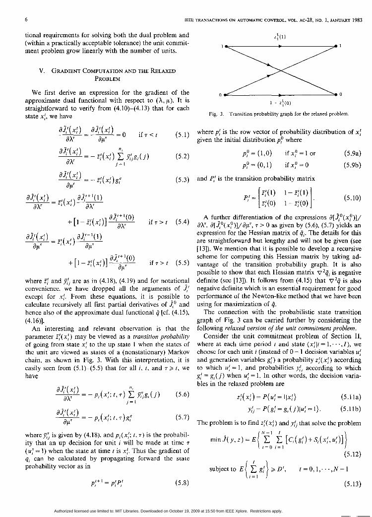
An interesting and relevant observation is that the parameter F,'(x:) may be viewed as a transition probability of going from state x: to the up state 1 when the states of the unit are viewed as states of a (nonstationaryj Markov chain. as shown in Fig. 3. With this interpretation, it is easily seen from (5.1)-(5.5) that for all i. r , and T >, r , we have

a$( x;) 17 1

ax = - p,(x,!; t , ~ ) JGgi( j ) (5.6) j = I

axt( .f) dPT

= - pi(x;; t. . )g; ( 5 -7)

where is given by (4.18), and p,(x:; t. T j is the probability that an up decision for unit i will be made at time T (u: = 1) when the state at time t is X:. Thus the gradient of q, can be calculated by propagating forward the state probability vector as in

Fig. 3. Transition probability graph for the relaxed problem

where p: is the row vector of probability distribution of xf given the initial distribution py where

pp = (1,O) if x: = 1 or (5 .sa)

pp=(O,I) i fxp=O (5.9b)

and P: is the transition probability matrix

if( 1) 1 - Ff( 1)

q ( 0 ) 1 - z;(o) P,' = I - (5.10)

A further differentiation of the expressions d[x.o(xO)]/ ax, a[xo(x:)]/ap7, T > 0 as given by (5.6), (5.7) yields an expression for the Hessian matrix of qi. The details for this are straightforward but lengthy and will not be given (see [13]). We mention that it is possible to develop a recursive scheme for computing this Hessian matrix by taking advantage of the transition probability graph. It is also possible to show that each Hessian matrix v2qi is negative definite (see [ 131). It follows from (4.15) that 0'4 is also negative definite which is an essential requirement for good performance of the Newton-like method that we have been using for maximization of 4.

The connection with the probabilistic state transition graph of Fig. 3 can be carried further by considering the following relaxed version of the unit commitment problem.

Consider the unit commitment problem of Section 11, where at each time period t and state { x f l i = I ; . - , Z } , we choose for each unit i (instead of 0 - 1 decision variables u: and generation variables g,!) a probability z:( x f ) according to which u: = 1, and probabilities I;: according to which g,' = g, ( j ) when u: = 1. In other words, the decision variables in the relaxed problem are

zf( x:) = P{ Uf = 11x;} (5.11a)

y;j=P{gf=g,(j)lu:=l) . (5.11b)

The problem is to find z:( xf ) and y/j that solve the problem

m i n . f ( y , z ) = ~ % / [C,(~~)+S,(X: ,U:)] "'- I

\ r = O i = l

(5.12)

> D l , t = O , I ; - - , N - l

(5.13)


BERTSEKAS et ai.: SCHEDULING OF LARGE-SCALE POWER SYSTEMS 7

Droblem

where E { - ) denotes expected value, and the probabilistic evolution of x f is specified by the transition probability graph of Fig. 3.

This problem is the same as the unit commitment problem except that we have expanded the set of feasible decisions to allow for randomized decisions.

Suppose that we have obtained an optimal solution (A, f i ) of the dual problem (3.4) via the approximation method of the previous section, and a corresponding set of multipliers ( 9 , i ) satisfymg (4.20)-(4.22). We will show that (9 ,2) is a solution of the relaxed unit commitment problem.

generated by the approximation method. Then ( A k , p k ) solves the approximate dual problem corresponding to ( y k , zk, d k ) , so from a necessary condition for optimality, we obtain

Indeed, let { ( h k , p k ) } and { ( y k , zk, dk)) be the SC3ClUenCeS

(5.16)

(5.17)

where all partial derivatives above are evaluated at (hk, pk, y k , zk, d k ) . Using the expression for @/aAt, a q / a p * obtained via (4.15), (4.16), (5.6), and (5.7), and the fact ( h k , p k ) + (A , f i ) , (ykr zk) + (j,Z^), we obtain from (5.15)

I n,

c p i ( x ! ; O , t ) 9 ; j g i ( j ) - D ‘ > 0 (5.18) i = l j = l

I p i ( x ! ; O , t ) g f - R ‘ > , O (5.19)

i = l

where pi (x ! ; 0, t ) is the probability that the decision made for unit i at time t corresponding to the randomized decision variables (p,Z ) will be to have the unit up (uf = 1). Thus (5.18), (5.19) simply say that ( 9 , i ) satisfies the constraints (5.13), (5.14) of the relaxed problem. Similarly, (5.16), (5.17) can be written as

I (5.20)

i = l

I (5.21)

Finally, if we form the Lagrangian function of the relaxed

we can verify easily using (4.20)-(4.22) that it is minimized at (9,Z). It follows from a well-known saddle-point theorem (see [5, pp. 144-1451) that ( 9 , 2 ) is an optimal solution to the relaxed problem, and furthermore the optimal value of this problem is equal to the dual optimal value q*.

It is important to note that to find a solution of the relaxed problem, it is not sufficient to find a solution ( A , f i ) of the dual problem and then minimize the Lagrangian function (5.22) with respect to ( y , z ) . This is due to the fact that minimizing pairs ( y , z ) of (5.22) need not satisfy the conditions (5.18)-(5.21). Thus solving the dual problem is by itself of little help in solving the relaxed problem. The point of view advanced in this paper is that the solution of the relaxed problem is far more important than the solution of the dual problem ( see Section VII). Therefore, a dual problem solution method such as the subgradient method used in [ 13, which does not simultaneously solve the relaxed problem, is inadequate for our purposes, while the approximation method that we have been using is fully satisfactory.

VI. AN ESTIMATE OF THE DUALITY GAP

In this section, we reformulate the relaxed version of the unit commitment problem as a linear programming problem. We then utilize basic linear programming results to show that there exists an optimal solution in which the number of units which have “relaxed” controls (i.e., unit commitment decisions that are noninteger) is at most equal to the number of demand and reserve constraints. This result is used to derive a bound on the duality gap associated with dualizing the unit commitment problem. This is done by bounding the increase in cost associated with modifying the relaxed solution into a feasible solution.2 Finally, since this increase in cost is independent of the number of units, we show that the duality gap goes to zero (in relative terms) as the number of units increases. An alternative and more general method for estimating the duality gap is given in [24].

To reformulate the relaxed problem as a linear programming problem, we show that selecting the z:(x!) and they:j is equivalent to assigning a probability to every possible sequence of controls (u i , g!) and that the cost and constraints can be formulated in terms of these sequences.

Let us enumerate all possible sequences of controls for each unit (this can be done since the values of uj are zero

must be zero or one; when applied to the unit commitment schedule it ’The term “feasible” when applied to a uni t means that the uf(.xf)

means that each unit’s schedule is feasible and that all constraints are satisfied.


8 IEEE TRANSACTIONS ON AUTOMATIC CONTROL. VOL. AC-28. NO. 1, JANUARY 1983

and one, and the only values we allow g: to assume are those of the breakpoints g i ( j ) ) and denote the k th such sequence by w:. Define

N - I

c,,= C { c i ( g : ) + S 1 ( x : , u f ) )

g:, = g:l(g;.u:)=%f? and (6.2)

(6.1)

6, = r ~ ( ~ ; ) l ( g : , u : ) = w : . (6.3)

t = O (g: . u:, = 5,; 3

Assign a “probability” pi , to each sequence .;” so that

C P i k = l . ( 6 . 4 ) k

If the z:(-xf) and the y:J have been selected, then the pix assigned to each sequence can be computed from

A- 1

P i k = ’:( xf)y:~ (6 3 ) t = O {g ; . u:, = h,!

where the xf correspond to the control sequence .;” and J,’~

is defined to be one if u: is zero. Equivalently, if thep,, are assigned to each sequence, we

can compute a consistent set of z:(x:) and J:~. This can be done recursively by computing the zp(xp) first, then the y:., then z!(xf>. etc. To compute zp(xp), simply add all the p f k which correspond to trajectories leaving x: via a decision of up = 1. If zp( x:) = 0, then the y: can be assigned arbitrarily; otherwise they can be computed by summing over all trajectories leaving x:, having up = 1. and having g: = g, ( j ) , and then normalizing by the probability zp( x; ).

Similarly. zf(xf) can be computed for any state whch can be reached via nonzero probability decisions: sum over the trajectories leading through that state and decision. and normalize by the probability of being in that state. This procedure leads to a set of z : ( x : ) and J:~ which are consistent with any assignment of pi,. The conclusion is that selecting the p l k is equivalent to selecting the {=:(x:). .I?‘ >.

Thus the relaxed unit commitment problem can be written as

,!

I

c P i k c l k (6 .6) P$A 1 = 1 k

subjectto C p i x = l , i = l ; . - . I (6.7) k

pi, > 0 (6.8) I

C p i k g : , > D r , t = O ; - . .N-1 (6.9) i = l k

I E p i k r / , 2 R‘, t = 0, - . . . N - 1. (6.10)

i = l k

This reformulation is clearly a linear programming problem with I + 2 N constraints.

If I > 2 N , then (compare with [5 , p. 1721) any basic feasible solution of the abme linear program has the propert)

that at least I - 2 N of the indexes i have precise& one pik positioe (and hence unity). To see this. note that any basic solution has at most I + 2 N variables positive. Each of the I constraints (6.7) requires at least one positive variable to satisfy it. The remaining 2 N basic variables are then associated with at most 2hr different units, leaving at most ( I - 2 N ) units i with exactly one positive variable p lk . If we consider the set of multipliers { z ; ( x f ) , y,:} corresponding to a basic feasible solution { p ik} as discussed earlier, we also find. based on the argument above, that at most 2 N of the multipliers z!(x:) , which correspond to states x: along which some variable p,, is positive, are neither zero or one.

If there exists any feasible solution to the linear program (6.6)-(6.10) (i.e., if operating all units at maximum output will satisfy demand and reserve constraints), then by not- ing that every feasible solution has finite cost? we can apply the fundamental theorem of linear programming to conclude that there exists an optimal basic solution to the linear program above.

Therefore it follows that there exists an optimal solution to the relaxed problem for which the schedules associated with I - 2N units are feasible with respect to the orignal unit commitment problem (i.e.. for whch the values of u: are zero or one). The important point to note is that at most 2 N units have schedules which do not meet the original integrality constraints and this bound is independent of the number of units. In fact, at most 2 N multipliers z!( x:) in an optimal solution to the relaxed unit commitment problem are noninteger, and thus a feasible solution to the unit commitment problem can be obtained by modifying the schedules of at most 2 N units.

Since the cost of t h s feasible solution overbounds the optimal unit commitment cost. and since the difference in the cost of the feasible and optimal relaxed solutions is constant. we can compute a bound on the duality gap which is independent of the number of units. The cost of the optimal unit commitment schedule grows as the number of units increases. Thus the duality gap, in relative terms, goes to zero as the number of units increases.

To determine the duality gap more precisely, we need to overbound the cost of modifying 2N relaxed schedules into 2 N feasible schedules. Clearly this cost is bounded by 2 N times the most expensive cost of modifying any one schedule. In Fig. 4, we plot the costs associated with operating a real unit (solid line) and the relaxed cost of operation (dashed line). Note that a demand and reserve feasible schedule which satisfies unit constraints can be obtained by turning the unit on as soon as possible and operating it at either the minimum output (if gf E [0, g , ] ) or at g! (if gff E [g, , E,]). The maximum cost associated-with this mod- ificatiin. since the generation cost is convex and increasing on [g, , E;]. is N times that associated with producing the minimum output instead of E > 0, where E is very small, plus the cost of starting up the unit.

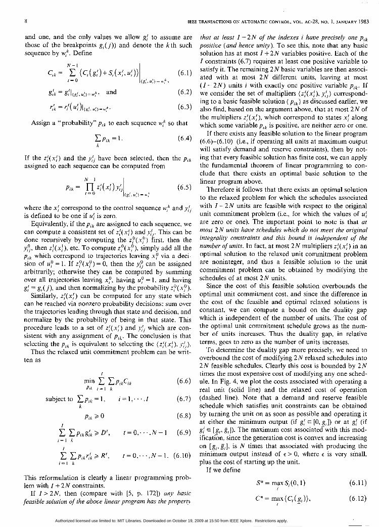
If we define

S* = maxS,(O, 1) (6.1 1)

C* = max { C, ( g i ) } : (6.12)

r

I -

~ ~ _ _ _ ~ ~


BERTSEKAS et al.: SCHEDULING OF LARGE-SCALE POWER S Y S T E ~ ~ S 9

L

L 9i g i

Fig. 4. Real and relaxed unit operation costs.

then the cost of modifying any unit schedule is less than S* + NC* and the cost of the feasible schedule is less than

4=4*+2N(S*+NC*) (6.13)

where q* is the cost of the relaxed (or dual) solution. The relative duality gap is thus bounded by

4 - q* 2N( s* + A T * ) -= (6.14)

4* q*

and since

limq* = + m , (6.15)

we have that the relative duality gap ( J * - q*)/q* [cf. (3.7)J goes to zero as the number of units I increases.

I -* x.

VII. OBTAINING A FEASIBLE UNIT COMMITMENT SCHEDULE

The preceding analysis has established that by solving the dual proljlem using the approximation method of Sec- tion IV, we obtain an optimal solution ($,i) of the relaxed unit commitment problem and that the corresponding optimal value is equal to the dual optimal value q*. We know from the analysis of Section VI that the duality gap is expected to be small and in fact becomes smaller in relative terms as the number of units increases. Therefore it foilows that the difference in the optimal values of the unit commitment problem and its relaxed version is.smal1. Thus if we were able to perturb slightly the relaxed optimal solution (p,z ) and obtain a feasible unit commitment schedule, then we could expect that this schedule would be close to being optimal. We next observe that once the decision variables uf are selected, then the up or down status of all units at each time is determined and the generation variables g,! can be chosen optimally by means of a simple standard economic dispatch calculation. Thus the variables $:, are not needed to provide near optimal values for the generation variables g,!.

There are two issues that arise in selecting the uf on the basis of the solution to the relaxed unit commitment problem [i.e., on the basis of the i : ( x f ) ] . The first is that, since we do not solve the dual problem exactly, many of the .2f(xf) may not have converged to zero or one, so there arises a question of deciding whether a particular unit i is “relaxed” or not at any particular time t on the basis of approximately optimal values of zf(x:). The second is that of how to modify a “relaxed” unit schedule. These issues

are resolved by treating a value of i f (x f ) which is within some small z of zero (one) as indicating that if unit i is in state xf at time l , then it should be up (down) in the next time period. Typically, less than 2N units are “relaxed” and for the remaining units, the if($) have converged to within 0.001 of zero or one by the time we have a satisfactory solution to the dual problem. An exception is when there is a class of units which are identical, in which case if one of these units is “relaxed,” all are “relaxed” and a large number of .’:(x;) may be far from zero or one. The solution to this type of problem falls under the second issue.

We modify a “relaxed” unit schedule into a feasible schedule by setting u f ( x f ) to one (zero) if z f (x f ) is over (under) a selected threshold. This threshold is selected so that the power generated by the units turned on is roughly equal to the “expected” power generated by these units in the relaxed solution. Note that this strategy handles classes of identical “relaxed” units in an intuitive manner: it turns on that fraction of units indicated by the if(x:).

VIII. COMPUTATIONAL RESULTS

A more sophisticated version of the preceding algorithm has been implemented in a Fortran code3 and was used to generate the results of this section. The implemented algorithm differs from the one discussed in this paper in two ways. First, we allow the imposition of minimum up and down time constraints on the operation of generators. The implemented algorithm produces a unit commitment schedule which satisfies all these constraints. Second, the implemented algorithm includes a variety of safeguards (e.g., against the Hessian. becoming indefinite due to finite precision arithmetic) and rules (e.g., step-size selection, convergence criteria for the approximate problems, etc.) which speed up convergence to the solution.

These safeguards and rules introduce parameters which allow one to tune the algorithm to the problem at hand. However, the overall method is quite insensitive to vari- ations in these parameters within a broad range. It should also be noted that the same parameters have been used for each combination of demand curve and generator set in Table I and that the same initial set of dual multipliers have been used for each example.

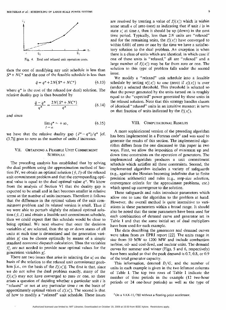
The data describing the generators and demand curves were taken from an EPRI report [22]. The units range in size from 50 MW to 1200 MW and include combustion turbine, oil- and coal-fired, and nuclear units. The demand curves for summer and winter (Figs. 5 and 6, respectively) have been scaled so that the peak demand is 0.7, 0.8, or 0.9 of the total generator capacity.

This information, denoted D/G, and the number of units in each example is given in the two leftmost columns of Table I. The top two rows of Table I indicate the number of time periods in the example (12 two-hour periods or 24 one-hour periods) as well as the type of

3 0 n a VAX-I 1/780 without a floating-point accelerator.


IO IEEE 'TRANSACTIONS ON AUTOMATIC CONTROL, VOL. AC-28, NO. 1, JAE.?.~&Y 1983

TABLE I SUMMARY OF COMPUTATIONAL RESULTS

--_______--_____==_=-_-_-=-.=_____.I-~ .=

XO. Cf 12 Tlrne Per iods

t i2ltS o's 24 Tine Periods

scnrer k'inter Summer n l n t e r

0.7 12, 3 .32%. :36 9, 0.35%, :2? 12, 0.36\, 1:46 11, 0.25%. 1:35

3 0 0.E 12, 5.60%. :34 9, 0.358, :27 1 C . 0.31%. 1:32 13, 0.15%. 1:57

0. 3 7 . 0 . 3 l P . :i2 9, 5 .12%. :26 -e, .~ 0.225. 2:13 10, 0.13%. 1:27

3.7 10, 0.29%. 1 :33 12 , 0.19%, 1:16 10, 0.319, 2:55 12, 0.295, 3:12

65 ' 2.8 L,;, 0.175, 1:Z'2 11, 0.168, 1 :56 8, 0.41%. 2:25 17, 0.16%. L:32

' 3.9 9, 0.313. : 5 5 7 , 0.135, :48 16. 0.131. 1:16 16. 0.21%. 4:36

0.7 10. 0 .06%. 2 : o : 6 , 0.17%. 1:41 11, 0.24%. 6:28 9, 0.24%. 5:21

12.2 ' 0.2 3 . 0 .26%. 1 :50 a, 0.349, 1:42 3 , 0.17%. 4:57 1 4 , 0.115. 7:26

0.3 7, 3.31%. 1:34 8 , 0.26%. 1:LO 1 5 , 0.09%. 7 :53 14, 0.10%. 7:21

0.7 8, 0.31%. 2:16 7, 0.09%. 2:38 12. 0.10€, 1O:57 13, 0.27%. 11:49

2 SJ 3.9 11, 0.3CS, 3:43 LC, 0.21%, 3:30 12, C.26b. 11:32 17, 0.09%, 12:12

- _ _ ~ _ _ _ - - - ~ ~ ' 0.0 9 , 3.C65. 3:OE 6 , 3.065. 2 :50 12, 0.47%. 15:43 il, 0.156, 9 :L8 _ _ _ ~ _ _ ~ ~ _ _ _ _

0.4 - 0 12 24

T IHE ihOURS)

Fig. 5 . Summer demand curve.

0.4 J I I I I 0 12 2 4

T ME i +OURS j

Fig. 6 . Winter demand c u n c

demand curve (i.e., summer or winter). Each entry in the table is a triple of numbers: the number of Newton steps required to solve the problem. an upper bound on suboptimality of the unit commitment schedule as given by ( j - Q)/Q where j is the cost of the feasible schedule computed and Q is the highest value of the dual functional obtained, and the CPU time required to solve the problem (min: s).

From this table we conclude that for large problems (over 100 units), we typically require 8 Newton steps or less and that the CPU time required to solve large problems (with 24 time steps) with this experimental (and as yet not optimized) code is roughly 4-6 &/lo0 units. The number of Newton steps required is an important quantity. since the computation of the Hessian matrix of the approximate dual functional dominates the computation time. Ths number ranges from 3- 14 steps and varies mainly

with the number of approximate dual problems that need to be solved (3 steps for 3 problems, 5-8 steps for 4 problems, and 9-14 steps for 5 approximate problems). The variation of computation time with problem data is quite small, however, and is not a cause for concern.

Table I also indicates the dependence of the computation time on problem size: roughly linear in the number of units and between linear and quadratic in the number of time steps. The dependence of the duahty gap on the problem size is somewhat less clear, but does roughly decrease with increasing numbers of units or time steps. Actually, the percentages shown in Table I are rather loose upper bounds on the actual value of the ratio ( j - J*)/J* which characterizes the degree of suboptimality of the feasible suboptimal schedule obtained. This is true not only because of the presence of a duality gap, but also because the dual functional q is maximized only approximately, and therefore the best dual value of 4 obtained is lower than the maximal value q* (and a fortiori J*). We found by experimentation that the difference ( q * - 4) can account for a substantial portion of the percentages shown in Table I.

The success achieved with our methodology in solving the optimal unit commitment problem is apparent from Table 1. Even the smallest problem in the table (30 units, 12 time periods) is twice as large as the largest optimal unit commitment problem that to our knowledge has ever been solved using other methods [ 11.

IX. SUMMARY AND EXTENSIONS

In t h s paper, we have introduced an algorithm for the solution of large ( loo+) unit commitment problems and shown that it can compute very accurate solutions (typically within 0.5 percent of optimal) very quickly (typically 4-6 min of CPU time per 100 units for 24-time-period problems). Whle the algorithm presented in Sections II-VI1 is valid only for state transition diagrams involving


BERTSEKAS et at.: SCHEDULING OF MGE-SCALE POWER SYSTEMS 1 1

two states, the algorithm implemented dows for the inch- [21] A. A. Goldstein. “Optimization of Lipschitz continuous functions,” sion of minimum up and down time constraints. [22] H. W. Zaininger, A. J. Wood, H. K. Clark, T. F. Laskowski, and

The algorithm is also applicable to scheduling power J. D. Burns. “Synthetic electric utilities systems for evaluating

system bo* and hydro units* For this [23] N. R. Sandell, Jr.. D. P. Bertsekas, J. J. Shaw, S. W. Gully, and R. purpose, a preliminary optimization phase is necessary to Gendron, “Ophmal scheduling of large scale hydrothermal power determine an optimal hydro generation schedule which is systems,” in Proc. IEEE Lorge Scale Syst. Conf.? Virginia Beach,

then used to determine the effective demand profile for the [24] D. P. Bertsekas and N. R. Sandell. Jr.. “Estimates of the duality gap VA, Oct. 1982.

thermal units. A separate paper deals with the details of for large scale separable integer programming problems.” in Proc. 1982 IEEE Conf. Decision and Conrr.. Miami Beach, FL. Dec. 1982.

Math. Programming, vol. 13, pp. 14-22, 1977.

advanced technologies,” Final Rep. EPRI-EM-285, 1977.

procedure [23].

REFERENCES

J. A. Muckstadt and S. A. Koenig. “An application of Lagrangian relaxation to scheduling in power-generation systems,” Operations Res., vol. 25, pp. 387-403, 1977. J. Gruhl, F. Schweppe, and M. Ruane, “Unit commitment scheduling of electric power systems,” in Systems Engineering for Pow8er: Status and Prospects, Eng. Foundation Conf.. L. H. Fink and K. Carlsen, Eds., Henniker, NH, 1975. A. Geoffrion, “Lagrangian relaxation for integer programming.” Math. Programming Stu@, vol. 2, pp. 82- I 14, 1974. L. S. Lasdon, Optimization Theov for Large Systems. New York: Macmillan, 1970. J. E. Shapiro, Mathematical Programming: Structures ami Alga- rithms. New York: Wiley, 1979.

put. Math. Math. Phys., vol. 9, pp. 14-??, 1969. B. T. Poljak, “Minimization of unsmooth functionals,” USSR Com-

M. Held, P. Wolfe, and H. Crowder, Validation of subgradient optimization,” Math. Program., vol. 6, pp. 62-88, 1974. D. P. Bertsekas, “Nondifferentiable optimization via approximation,” Math. Programming Study, vol. 3, pp. 1-25, 1975. - , “Approximation procedures based on the method of multi-

E;. lien,” J . Optimiz. Theoy Appl., vol. 23, pp. 487-510. 1977.

for constrained minimization,” in Proc. 1972 IEEE Conf. Decision W. Kort and D. P. Bertsekas, “A new penalty function method

Contr., New Orleans, LA, 1972, pp. 162-166. D. P. Bertsekas, “Projected Newton methods for optimization problems with simple constraints,” Lab. Inform. Decision Syst., M.I.T.. Cambridge, MA, Rep. R-1025, Aug. 1980; see also SIAM J . Contr. Optimiz., vol. 20, no. 2, pp. 221-246, 1982. G. S. Lauer, D. P. Bertsekas, N. R. Sandell, Jr., and T. A. Posbergh, “Solution of large-scale optimal unit commitment problems,” IEEE

G. S. Lauer, D. P. Bertsekas, and N. R. Sandell, Jr., “Optimal Trans. Power App. Syst., vol. PAS-101, pp. 74-86, 1982.

stochastic operations scheduling first annual report,” TR-108, AI- phatech, Inc., Burlington, MA, Rep. TR-108, Sept. 1980. V. H. Nguyen and J. J. Strodiot, “On the convergence rate of a penalty function method of exponential type,” J . Optimiz. Theov

D. P. Bertsekas, Constrained Optimization and Lagrange Multiplier Methods. New York: Academic, 1982. D. P. Bertsekas and S. K. Mitter, “A descent numerical method for optimization problems with nondifferentiable cost functionals,” SIAM J . Contr. Optimiz., vol. 11, pp. 637-652, 1973. C. Lemarechal, “An algorithm for minimizing convex functions,” in PFOC. IFIP Congr. 1974, J. L. Rosenfeld, Ed. Amsterdam, The Netherlands: North-Holland, 1974, pp. 552-557. N. Z. Shor, “Convergence of a gradient method with space dilation in the direction of the difference between two successive gradients,” Cybernetics, vol. 1 1, pp. 564-570, 1975. R. Mifflin, “An algorithm for constrained optimization with semi- smooth functions,” Math. Operations Res., vol. 2, pp. 191-207, 1977. P. Wolfe, “A method of conjugate subgradients for minimizing nondifferentiable functions,” Math. Programming St*, vol. 3, pp.

Appl., VOI. 27, pp. 495-508, 1979.

145-173, 1975.

Dimitri P. Bertsekas (S’70-SM77), for a photograph and biography, see p. 616 of the June 1982 issue of this TRANSACTIONS.

Gregory S. Lauer (S’77-M79) was born in Bos- ton. MA, in 1953. He received the B.S.E.E. and M.S.E.E. degrees from the University of Notre Dame, IN, in 1975 and 1976, and the Ph.D. degree in electrical engineering and computer science from the Massachusetts Institute of Tech- nology, Cambridge. in 1979.

He has worked at Alphatech, Inc., Burlington, MA, since 1979. He has done research and is interested in the areas of optimization, estima- tion, detection, and communication.

Dr. Lauer is a member of Eta Kappa Nu and Sigma Xi.

Nils R. Sandell, Jr. (S’70-M74), for a photograph and biography, see p. 838 of the August 1982 issue of this TRANSACTIONS.

Thomas A. Posbergh (S’74-M78-M79) was born in Elizabeth, NJ, on April 24, 1954. He received the B.S. degree from New Jersey Institute of Technology, Newark, in 1976 and the S.M. degree from the Massachusetts Institute of Tech- nology. Cambridge, in 1979, both in electrical engineering.

From 1976 to 1979 he was associated with the Charles Stark Draper Laboratory, Cambridge, MA. From I979 to 1981 he was a Staff Engineer with Alphatech, Inc., Burlington. MA. At present

he is employed by the U.S. Army Armament Research and Development Command, Dover, NJ. His current interests include decision making under uncertainty, stochastic systems, numerical methods, and micro- processor implementation of control algorithms.


Documents

IEEE CO~TROL, VOL. NO. Optimal Large-Scale Power