IEEE TRANSACTIONS ON COMMUNICATIONS, VOL. XX, NO. XX, … · IEEE TRANSACTIONS ON COMMUNICATIONS, VOL. XX, NO. XX, APRIL 2018 1 A Novel 3D Non-Stationary Wireless MIMO Channel Simulator

IEEE TRANSACTIONS ON COMMUNICATIONS, VOL. XX, NO. XX, APRIL 2018 1

A Novel 3D Non-Stationary Wireless MIMOChannel Simulator and Hardware Emulator

Qiuming Zhu, Member, IEEE, Hao Li, Yu Fu, Cheng-Xiang Wang, Fellow, IEEE, Yi Tan, Xiaomin Chen,Qihui Wu, Senior Member, IEEE

Abstract—In this paper, a new WINNER+ based three di-mensional (3D) non-stationary geometry-based stochastic model(GBSM) for multiple-input multiple-output (MIMO) channels isproposed, as well as extended evolving algorithms of time-variantchannel parameters. Meanwhile, important statistical propertiesof the channel model, i.e., time-variant autocorrelation function(ACF), time-variant cross-correlation function (CCF), and time-variant Doppler power spectrum density (DPSD) are derivedand analyzed. Moreover, we propose an efficient hardwareimplementation method, namely sum-of-frequency-modulation(SoFM) method, to generate non-stationary channel coefficients.By utilizing a compact hardware architecture with SoFM mod-ules, the proposed 3D non-stationary GBSM is realized on afield-programmable gate array (FPGA) hardware platform. Sim-ulations and hardware measurement results demonstrate that ourproposed channel simulator and emulator can get more accurateand realistic Doppler frequency than those of the existing models.In addition, hardware measurements of statistical propertiesare also consistent well with the corresponding theoretical ones,which verifies the correctness of both the hardware emulationscheme and theoretical derivations.

Index Terms—3D non-stationary GBSM, MIMO channelmodel, WINNER+ channel model, hardware emulation, sum-of-frequency-modulation method, statistical properties.

I. INTRODUCTION

MULTIPLE-INPUT multiple-output (MIMO) technolo-gies have widely been used to improve spectral effi-

ciency and link reliability significantly [1]–[3]. By utilizingthe cross-polarized antenna and spatial resource, the three-dimensional (3D) MIMO technology has also become a

Manuscript received October 9, 2017; revised March 1, 2018; accepted March27, 2018. This work was supported by the EU H2020 ITN 5G Wireless project(Grant No. 641985), EU H2020 RISE TESTBED project (Grant No. 734325),EU FP7 QUICK project (Grant No. PIRSES-GA-2013-612652), EPSRCTOUCAN project (Grant No. EP/L020009/1), Natural Science Foundation ofChina (Grant No. 61631020), Postdoctoral Fund of Jiangsu Province (GrantNo. 1601017C), and Fundamental Research Funds for the Central Universities(Grant No. NS2016044 and NJ20160027).

Q. Zhu is with College of Electronic and Information Engineering, NanjingUniversity of Aeronautics and Astronautics, Nanjing, 211106, China. He is alsowith the Institute of Sensors, Signals and Systems, School of Engineering &Physical Sciences, Heriot-Watt University, Edinburgh EH14 4AS, U.K. (e-mail:[email protected]).

H. Li, X. Chen, and Q. Wu are with College of Electronic and InformationEngineering, Nanjing University of Aeronautics and Astronautics, Nanjing,211106, China (e-mail: {lihao xc, chenxm402, wuqihui}@nuaa.edu.cn).

Y. Fu and Y. Tan are with the Institute of Sensors, Signals and Systems,School of Engineering & Physical Sciences, Heriot-Watt University, EdinburghEH14 4AS, U.K. (e-mail: {y.fu, yi.tan}@hw.ac.uk).

C.-X. Wang (corresponding author) is with the Mobile CommunicationsResearch Laboratory, Southeast University, Nanjing, 211189, China. He is alsowith the Institute of Sensors, Signals and Systems, School of Engineering &Physical Sciences, Heriot-Watt University, Edinburgh EH14 4AS, U.K. (e-mail:[email protected]).

promising solution for the fifth generation (5G) communicationsystems [4], [5]. However, all these benefits can only beachieved with the thorough understanding of propagation char-acteristics of the underlying channel. Measurement campaignshave proved that the stationary assumption is only valid fora short time interval [6] and it would be even shorter in highmobility scenarios, such as high speed train (HST) channels[7], [8] and vehicle-to-vehicle (V2V) channels [9]. Therefore,the 3D MIMO and non-stationary aspects should be taken intoaccount when designing channel models of 5G systems.

There are limited non-stationary channel models that havebeen reported in the literature [10]–[24]. Those models can beclassified as deterministic models [10], [11], non-geometricalstochastic models (NGSMs) [12], [13], and geometry-basedstochastic models (GBSMs) [14]–[24]. The deterministicmodels, as an alternative model in METIS [10] and the 3rdGeneration Partnership Project (3GPP) 3D channel model [11],are based on the ray-tracing method. Although with highaccuracy, deterministic channel models need a detailed digitalmap with specific trajectories and their simulations are alsovery time consuming. The NGSMs [12], [13] characterize thechannel in a completely stochastic way. As all parametersare extracted from measurements, NGSMs do not includegeometrical information and cannot be used for system-levelsimulations.

To guarantee a good tradeoff between the complexity andaccuracy of the model, GBSMs were proposed for both sta-tionary channel modeling [25]–[30] and non-stationary channelmodeling [14]–[24]. For example, a time evolving channelmodel based on the WINNER II model [30] was proposedin [14] and [15], where the channel was split into severalindependent segments and the WINNERII model was appliedin each segment. The two dimensional (2D) non-stationarychannel models for HST and massive MIMO channels canbe found in [16], [17], and [18], respectively. The authors in[16] and [18] assumed that the scatterers were distributed onmultiple ellipses based on different delays and the channelstates were updated by tracking the instantaneous positions ofthe mobile relay (MR) [16] or the mobile station (MS) [18]. Themulti-bounced scatterers were also taken into account by a 2Dtwin-cluster approach in [17], which made the model becomemore realistic. A 3D non-stationary channel model under theV2V scenario was proposed in [19], where scatterers weredistributed as two regular spheres and moved together withthe vehicles. The authors considered the random movement ofthe MS and described the trajectory as a Brownian process in[20]. Moreover, the 3D twin-cluster approach was adopted in

2 IEEE TRANSACTIONS ON COMMUNICATIONS, VOL. XX, NO. XX, APRIL 2018

[21] and [22] to model 3D non-stationary mobile channels andmassive MIMO channels, respectively.

It should be highlighted that the aforementioned non-stationary GBSMs [14]–[22] can be viewed as the modifiedGBSMs with time-variant channel parameters. The major effortof these models focused on the evolving algorithms of channelparameters along time [14]–[17], [19]–[21] or along both timeand antenna location [18], [22]. However, we have found thatthe output fading phases generated by these models are notaccurate, which results in the output Doppler power spectrumdensity (DPSD) not consistent with the corresponding analyticalone [23]. Some latest works such as [24] and [23] have indeedrealized this shortcoming and considered the right formulationof the time-varying phase. However, the authors in [24] onlyconsidered 2D scattering environments and did not give thecomputation method of time evolving channel parameters. Theprevious work of our group [23] proposed a new 3D non-stationary channel model with the accurate fading phase andDPSD for the first time, but it did not give the detailed statisticalproperties of the proposed model.

Compared with field tests, the hardware emulation method isvisible, controllable, and repeatable. It provides better real-timeemulation and is more efficient than the software simulationmethod. Thus, channel emulator has become a very importanttool to test and evaluate future wireless systems. There areseveral commercial channel emulators in the market [31]–[33].However, they are very expensive and mostly designed forstandard channel models. Meanwhile, various academic workson hardware emulation were done in [34]–[39], but most ofthem focused on stationary channels. A non-stationary single-input single-output (SISO) channel emulator was proposed in[40], where the channel parameters were calculated periodicallyby the Agilent advanced design system (ADS) software andthen an instrument (E4432B) was used to generate channelcoefficients. For the limited number of hardware interfaces, thismethod can only support SISO channel emulations. Recently,researchers in [41] developed a MIMO channel emulator onNI USRP-Rio 2953 platform. However, they took the non-stationarity into account only by assuming several independentstationary regions and switched channel states among theseregions. To the best of our knowledge, there is no channelemulator designed for non-stationary channel models thatconsider the continuity of channel states between differentstationary regions. This paper aims to fill the above researchgaps.

Overall, the major contributions and novelties of this paperare summarized as follows:

1) This paper proposes an improved 3D non-stationary wide-band GBSM for MIMO channels, as well as the extended timeevolving algorithms of estimating channel parameters. The newmodel originates from the 3D stationary WINNER+ channelmodel [29], but differs from the non-stationary models in [14]–[22] by generating accurate fading phases and guarantees morerealistic Doppler frequency and DPSD.

2) By taking the impact of time-variant path delays intoaccount, a new 3D correlation function is derived for the pro-posed 3D non-stationary GBSM. Moreover, the expressions oftime-variant autocorrelation function (ACF), cross-correlation

function (CCF), and DPSD are also derived. These resultscan be used to validate the software simulation and hardwareemulation.

3) With the new idea of sum-of-frequency-modulation(SoFM) method, an efficient hardware implementation methodtailored for the proposed non-stationary channel simulatoris proposed. On this basis, a compact channel emulationscheme with low complexity on a field-programmable gatearray (FPGA) platform is developed and validated.

The rest of this paper is organized as follows. In Section II,the original 3D stationary WINNER+ channel model is brieflyintroduced. Section III proposes our new 3D non-stationarychannel model, as well as the extended algorithms of estimatingchannel parameters. In addition, the theoretical results of ACF,CCF, and DPSD for our model are derived. In Section IV, anefficient hardware implementation method and the compacthardware structure based on the SoFM module are presented.In this section, the hardware resource consumption is alsogiven and analyzed. The test results of the channel emulatorare presented in Section V. Finally, the conclusions are givenin Section VI.

II. A 3D STATIONARY GBSM FOR MIMO CHANNELS

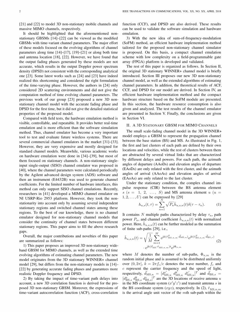
The small scale-fading channel model in the 3D WINNER+model employs a GBSM to represent the propagation channelbetween the base station (BS) and MS. As illustrated in Fig. 1,the first and last clusters of each path are defined by their ownlocations and velocities, while the rest of clusters between themare abstracted by several virtual links that are characterizedby different delays and powers. For each path, the azimuthangles of departure (AAoDs) and elevation angles of departure(EAoDs) are only related with the first cluster, and the azimuthangles of arrival (AAoAs) and elevation angles of arrival(EAoAs) are only related to the last cluster.

Under the stationary condition, the complex channel im-pulse response (CIR) between the BS antenna elements (s = 1, 2, . . . , S) and MS antenna element u (u =1, 2, . . . , U) can be expressed by [29]

hu,s(t, τ) =N∑n=1

√Pnhu,s,n(t)δ(τ − τn). (1)

It contains N multiple paths characterized by delay τn, pathpower Pn, and channel coefficient hu,s,n(t) with normalizedpower. Here, hu,s,n(t) can be further modeled as the summationof finite sub-paths [29], i.e.,

hu,s,n(t) =

√1

M

M∑m=1

ejk(rTMS,n,m·~dMS,u)ejk(rTBS,n,m·~dBS,s)

· ejk(~vMS·rMS,n,m)tejΦn,m

(2)

where M denotes the number of sub-paths, Φn,m is therandom initial phase and is assumed to be distributed uniformlyover (0, 2π], k = 2πfc/c denotes the wave number, fc andc represent the carrier frequency and the speed of light,respectively, ~dMS,u = [dx

′

MS,u dy′

MS,u dz′

MS,u]T and ~dBS,s =

[dxBS,s dyBS,s d

zBS,s]

T are the 3D locations of receive antenna uin the MS coordinate system (x′y′z′) and transmit antenna s inthe BS coordinate system (xyz), respectively. In (2), rMS,n,m

is the arrival angle unit vector of the mth sub-path within the

ZHU et al.: A NOVEL 3D NON-STATIONARY MIMO CHANNEL SIMULATOR AND HARDWARE EMULATOR 3

Fig. 1. BS and MS angle parameters in the 3D GBSM.

nth path with AAoA φAAoAn,m and EAoA θEAoA

n,m , and is definedby [21]

rMS,n,m =

sin(θEAoAn,m ) cos(φAAoA

n,m )sin(θEAoA

n,m ) sin(θEAoAn,m )

cos(φEAoAn,m )

(3)

while rBS,n,m is the departure angle unit vector of the mthsub-path within the nth path with AAoD φAAoD

n,m and EAoDθEAoDn,m , and is given by

rBS,n,m =

sin(θEAoDn,m ) cos(φAAoD

n,m )sin(θEAoD

n,m ) sin(θAAoDn,m )

cos(φEAoDn,m )

. (4)

The theoretical Doppler frequency of the mth sub-path withinthe nth path in (2) can be calculated by [29]

fn,m =‖~vMS‖ cos(θvMS,n,m

)

cfc (5)

where ~vMS and ‖~vMS‖ denote the vector and magnitude of theMS velocity, respectively. Here, θvMS,n,m

is the angle between~vMS and rMS,n,m, and can be expressed as

θvMS,n,m= arccos

( ~vMSrMS,n,m

‖vMS‖‖rMS,n,m‖

). (6)

Submitting (6) into (5) and holding ‖rMS,n,m‖ = 1, we canobtain

fn,m = k~vMSrMS,n,m

2π. (7)

It should be noticed that the third exponential item in (2),denoted as ψn,m(t) = 2πfn,mt = k(~vMSrMS,n,m)t, representsthe corresponding phase caused by the Doppler frequency.According to the relationship between the frequency and phase,the output Doppler frequency can be calculated as

f ′n,m =1

2π

dψn,m(t)

dt= k

~vMSrMS,n,m

2π(8)

which equals to the corresponding theoretical one fn,m as in(7).

III. A NEW 3D NON-STATIONARY GBSM ANDSTATISTICAL PROPERTIES

A. The proposed 3D non-stationary GBSM

The CIR of our proposed 3D non-stationary GBSM can beexpressed as

hu,s(t, τ) =

N(t)∑n=1

√Pn(t)hu,s,n(t)δ(τ − τn(t)) (9)

where

hu,s,n(t)=

√1

M

M∑m=1

ejk(rTMS,n,m(t)~dMS,u(t))

· ejk(rTBS,n,m(t)~dBS,s(t))

· ejk∫ t0

(~vzn,MS·rMS,n,m(t′))dt′ejΦn,m .

(10)

Here, channel model parameters in (9) and (10) such asN(t), Pn(t), τn(t), rTMS,n,m(t), ~dMS,u(t), rTBS,n,m(t), and~dBS,s(t) are all time-variant, which capture the non-stationaritycharacteristics of the underlying channel.

The theoretical Doppler frequency of non-stationary channelswould change over time and can be denoted as fn,m(t) =k~vMSrMS,n,m(t)/2π. Most of the existing non-stationary chan-nel models [14]–[22] directly used the phase ψ′n,m(t) =k~vMSrMS,n,m(t)t to substitute ψn,m(t). However, in this case,the output time-variant Doppler frequency can be proved as

f ′n,m(t) =1

2π

dψ′n,m(t)

dt

=k~vMSrMS,n,m(t)

2π+

t

2π

dk~vMSrMS,n,m(t)

dt6= fn,m(t)

(11)

which does not agree with the corresponding theoreti-cal one. To overcome this problem, we use ψn,m(t) =

k∫ t

0(~vMSrMS,n,m(t))tdt instead of ψ′n,m(t) to represent the

effect of the Doppler frequency [23]. It’s easy to demonstratethat the output Doppler frequency of our proposed model equalsto the theoretical one, i.e, 1

2πdψn,m(t)

dt = fn,m(t). In addition,unlike the WINNER+ model, we take the movement of clusterZn into account by replacing item ~vMS of (2) with the relativevelocity between the MS and cluster Zn as

~vZn,MS =[vxZn,MS v

yZn,MS v

zZn,MS

]=[vxMS − vxZn v

yMS − v

yZn

vzMS − vzZn] (12)

where ~vMS=[vxMS vyMS vzMS] and ~vZn=[vxZn vyZn vzZn ]denote the velocity vectors of the MS and cluster Zn, respec-tively. Moreover, it should be mentioned that the new modelalso supports time-variant movements situation and this can beguaranteed by replacing ~vZn,MS with ~vZn,MS(t). The detaileddefinitions of channel parameters can be found in Table I.

B. Time-variant channel parameters

1) Path number

The number of valid paths is time-variant due to the movementsof the MS and clusters, which means some clusters will disappearand some new clusters will appear. This was mentioned in [29]as the birth-death process. Let us set the birth and death rates


DBS,An(t) =√DBS,An

2(t−∆t)+(‖~vAn‖∆t)2+2DBS,An(t−∆t) sin θEAoD

n (t−∆t)‖~vAn‖∆t cos(φAAoD

n (t−∆t)−θAn) (16)

DZn,MS(t) =√DZn,MS

2(t−∆t)+(‖~vZn,MS‖∆t)2+2DZn,MS(t−∆t)sinθEAoAn (t−∆t)‖~vZn,MS‖∆tcos(θZn,MS−φAAoA

n (t−∆t)) (17)

DLOS(t)=

√D2

LOS(t−∆t)+(‖~vMS‖∆t)2 +D2

LOS(t−∆t) + (‖~vMS‖t)2 −D2

LOS(t0)

t∆t (18)

TABLE I

DEFINITION OF PARAMETERS.

N(t) number of valid propagation pathsPn(t), τn(t) power and delay of the nth path, respectively~dBS,s(t), ~dMS,u(t)

3D location vectors of the BS antennas s andMS antenna u, respectively

~vMS, ~vAn , ~vZn3D velocity vectors of the MS and clustersAn,Zn, respectively

rBS,n(t), rMS,ndeparture and arrival angle unit vectors of thenth path, respectively

rBS,n,m(t), rMS,n,mdeparture and arrival angle unit vectors of themth ray within the nth path, respectively

θEAoDn (t), φAAoD

n (t),θEAoAn (t), φAAoA

n (t)mean angles of the EAoD, AAoD, EAoA, andAAoA of the nth path, respectively

θEAoDn,m (t), φAAoD

n,m (t),

θEAoAn,m (t), φAAoA

n,m (t)EAoD, AAoD, EAoA, and AAoA of the mthray within the nth path, respectively

DLOS(t), DBS,An (t),DZn,MS(t)

distances of BS to MS, BS to cluster An, andMS to cluster Zn, respectively

as λG and λR, respectively, and model the evolution of pathnumber as a Markov process [37]. The movement of clustersin a realistic environment is random and unknowable, while theaverage velocity can be obtained by the measurement campaign. Itis assumed that the average velocity of cluster An, n = 1, . . . , N(or Zn, n = 1, . . . , N) is ~vA (or ~vZ). Thus, the mean survivalprobability of each path during time interval ∆t can becalculated by the average velocities as [22]

Premain =exp(−λR(Pc(‖~vA‖+‖~vZ‖)∆t+‖~vMS‖∆t)) (13)

where Pc denotes the percentage of movement, ‖~vA‖, ‖~vZ‖are the magnitudes of mean velocities of cluster An and Zn,respectively, and ‖~vMS‖ is the velocity of MS. In order tokeep the average number of valid paths constant, the numberof newly generated paths Nnew(t) is modeled by a Poissonprocess with the expectation as

E{Nnew(t)} =λGλR

(1− Premain). (14)

Combining (13) with (14), we can obtain the average pathnumber as

E{N(t)}=N(t−∆t)Premain+E{Nnew(t)}=λGλR

(15)

which only depends on the parameters of birth and death rates.2) Path distances

With the movements of the MS and clusters, the distancesbetween the MS, BS, and clusters will change over time.

Measurement campaigns in [7] have shown that the stationaryinterval is very short, i.e., 9 ms for 80 % and 20 ms for60 %. In this paper, all velocities are assumed to keep constantwithin the short stationary interval. All velocities are assumedto keep constant during the short analytical time interval andthe initial distances between the BS (MS) and cluster An

(Zn) are obtained by a measurement campaign or generationrandomly. We have proved that the instantaneous distances attime instant t can be calculated from the following iterativealgorithms (16)–(18),where θAn = arctan(vyAn/v

xAn

) andθZn,MS = arctan(vyZn,MS/v

xZn,MS).

3) Delays and powers

For the nth valid path, the total delay at time instant t equalsto the summation of the delay of the first bounce, delay of thevirtual link, and delay of the last bounce, and is also determinedby the total distance as

τn(t)=DBS,An(t) +DZn,MS(t) +DAn,Zn(t)

c

=DBS,An(t) +DZn,MS(t)

c+ τn(t)

(19)

where τn(t) denotes the equivalent delay of virtual link andcan be updated by a first-order filtering method [22],

τn(t) = τn(t−∆t)e− ∆tτdec + (1− e

− ∆tτdec )X (20)

where X ∼ U [DLOS(t)/c, τmax], τmax and τdec denote themaximum delay and decorrelation speed of time-variant delays.The average power of this path can be calculated by themeasurement-based method [29] as,

P ′n(t) = e−τn(t)

1−rDSrDSσ

DS × 10−ξn10 (21)

where ξn, rDS, and rDS denote the shadow term, delaydistribution, and delay spread, respectively. Finally, the totalpower of all paths should be normalized as

Pn(t) = P ′n(t)/

N(t)∑n=1

P ′n(t). (22)

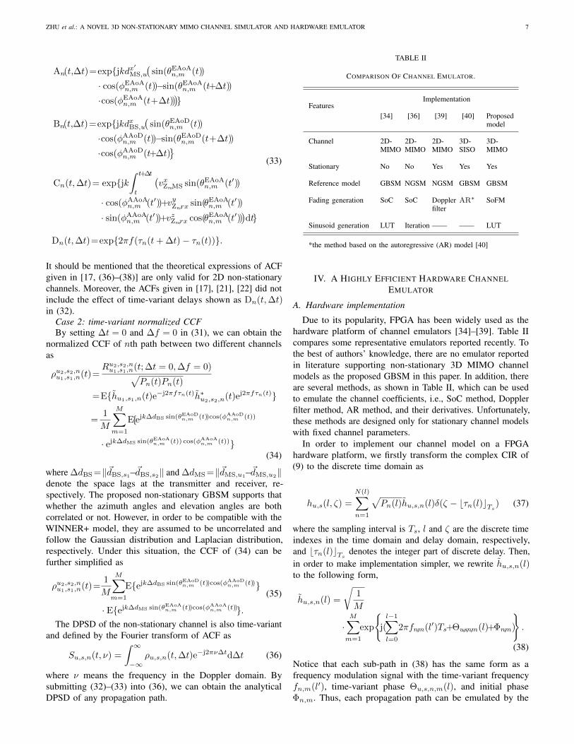
In order to illustrate the time-variant properties of pathnumber, delays, and powers, we set the simulation environmentas the C2-NLoS scenario in WINNER+ model [29]. The birthrate, death rate, and the percentage of movement can be foundin Table I of [27] as λG = 0.8 /m, λR = 0.04 /m, and Pc =0.3. The simulation parameters of initial or newly generatedpaths are as follows, ‖~vMS‖ = 80 km/h, ‖~vA‖ = 30 km/h,‖~vZ‖ = 30 km/h, DBS,An(t0) = 50 m, DZn,MS(t0) = 50 m,


(a)

0 2 4 6 8 10Time,t(s)

10

15

20

25

The

number

ofvaild

paths

(b)

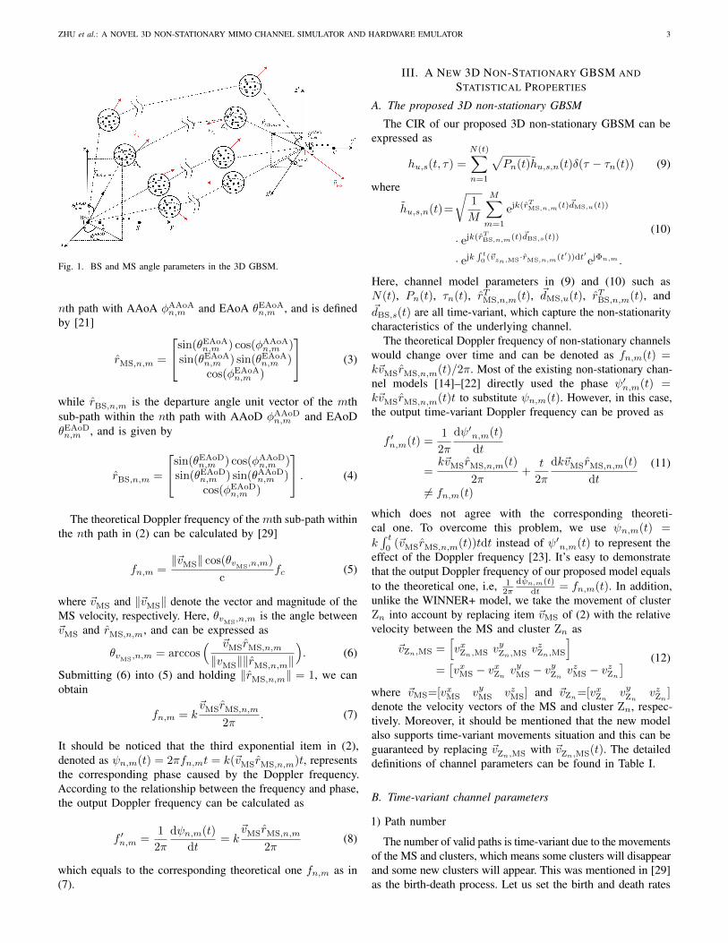
Fig. 2. (a) Time-variant PDP and (b) the number of valid paths of the proposed 3D non-stationary GBSM at different times (C2-NLoS scenario, ‖~vMS‖ = 80 km/h,‖~vA‖ = 30 km/h, ‖~vZ‖ = 30 km/h, DBS,An (t0) = 50 m, DZn,MS(t0) = 50 m, and DLOS(t0) = 100 m).

θEAoDn (t)=

arctan

√(DBS,An (t0) sinθEAoD

n (t0))2+(‖~vAn‖t)2+2DBS,An(t0)sinθEAoD

n (t0)‖~vAn‖t cos(φAAoD

n (t0)−θAn )

DBS,An (t0) cos θEAoDn (t0) , (a)

if 0≤θEAoDn (t0)≤ π

2

π−arctan

√(DBS,An (t0) sinθEAoD

n (t0))2+(‖~vAn‖t)2+2DBS,An(t0)sinθEAoD

n (t0)‖~vAn‖t cos(φAAoD

n (t0)−θAn )

DBS,An (t0) cos θEAoDn (t0) , (b)

if π2 <θ

EAoDn (t0)≤π

(23)

θEAoAn (t)=

arctan

√(DZn,MS(t0) sin θEAoA

n (t0))2+(‖~vZn,MS‖t)2+2DZn,MS(t0)sinθEAoAn (t0)‖~vZn,MS‖t cos(θZn,MS−φAAoA

n (t0))

DZn,MS(t0) cos θEAoAn (t0) , (a)

if 0≤θEAoAn (t0)≤π2

π−arctan

√(DZn,MS(t0)sin θEAoA

n (t0))2+(‖~vZn,MS‖t)2+2DZn,MS(t0)sinθEAoAn (t0)‖~vZn,MS‖t cos(θZn,MS−φAAoA

n (t0))

DZn,MS(t0) cos θEAoAn (t0) , (b)

if π2<θ

EAoAn (t0)≤π

(24)

φAAoDn (t)=

φAAoDn (t)=φAAoD

n (t0)+αAAoDn (t) , φAAoD

n (t0)∈(0, π], θAn∈(φAAoDn (t0), φAAoD

n (t0)+π) (a)φAAoDn (t)=φAAoD

n (t0)−αAAoDn (t), φAAoD

n (t0)∈(0, π], θAn∈(0, φAAoDn (t0))∪(φAAoD

n (t0)+π, 2π) (b)φAAoDn (t)=φAAoD

n (t0)−αAAoDn (t), φAAoD

n (t0)∈(π, 2π], θAn∈(φAAoDn (t0)− π, φAAoD

n (t0)) (c)φAAoDn (t)=φAAoD

n (t0)+αAAoDn (t), φAAoD

n (t0)∈(π, 2π], θAn∈(0, φAAoDn (t0)− π)∪(φAAoD

n (t0), 2π) (d)

(25)

φAAoAn (t)=

φAAoAn (t)=φAAOA

n (t0)+γAAOAn (t) , φAAoA

n (t0)∈(0, π], θAn∈(φAAOAn (t0), φAAOA

n (t0)+π) (a)φAAoAn (t)=φAAOA

n (t0)−γAAOAn (t), φAAOA

n (t0)∈(0, π], θAn∈(0, φAAOAn (t0))∪(φAAOA

n (t0)+π, 2π) (b)φAAoAn (t)=φAAOA

n (t0)−γAAOAn (t), φAAOA

n (t0)∈(π, 2π], θAn∈(φAAoAn (t0)− π, φAAOA

n (t0)) (c)φAAoAn (t)=φAAOA

n (t0)+γAAOAn (t), φAAOA

n (t0)∈(π, 2π], θAn∈(0, φAAOAn (t0)− π)∪(φAAOA

n (t0), 2π) (d)

(26)

DLOS(t0) = 100 m, ‖~vAn‖ and ‖~vZn‖ ∼ U(0, 60) km/h, andall directional parameters are generated randomly. Fig. 2 (a)gives the time-variant 3D power delay profile (PDP) of onesimulation trial from our non-stationary channel model. Inorder to highlight time-variation of path delays, y axis adoptsthe absolute delay. As the MS moves away from the BS, wecan see that the delay of each path increases and the minimumvalue is limited by DLOS(t)/c. Fig. 2 (a) also demonstratesthe disappearance and appearance of valid paths over time, aswell as dynamic changes of delays and powers. Meanwhile,Fig. 2 (b) calculates the total number of valid paths at different

times. It is showed that the number is fluctuated around initialvalue and the average value is about 19.9, matching well withthe result of (15).

4) Angles for the 3D channel model

Measurement results in [29] have indicated that the marginaldistribution of power angular spectrum (PAS) in the elevationplane follows the Laplacian distribution, while the PAS in theazimuth plane follows the truncated Gaussian distribution. Inthis paper, the angles of initial paths or newly generated pathsare following those two distributions. In order to keep


αAAoDn (t) =arccos

DBS,An(t0) sin θEAoDn (t0) + ‖~vAn

‖t cos(φAAoDn (t0)− θAn)√

(DBS,An(t0)sinθEAoDn (t0))2+(‖~vAn

‖t)2+2DBS,An(t0) sin θEAoDn (t0)‖~vAn

‖t cos(φAAoDn (t0)−θAn)

(27)

γAAoAn (t)=arccos

DZn,MS(t0) sin θEAoAn (t0)+‖~vZn,MS‖t cos(θZn,MS−φAAoA

n (t0))√(DZn,MS(t0)sinθEAoA

n (t0))2+(‖~vZn,MS‖t)2+2DZn,MS(t0)sin θEAoAn (t0)‖~vZn,MS‖t cos(θZn,MS−φAAoA

n (t0)). (28)

PAS distributions unchanged over time, we only trackthe mean angles of EAoD, EAoA, AAoD and AAoA. Basedon geometrical relationships, the time evolving functions of themean angles of EAoD and EAoA are derived as (23) and (24),where θEAoD

n (t0), φAAoDn (t0), θEAoA

n (t0), and φAAoAn (t0)

denote the initial values of the EAoD, AAoD, EAoA, andAAoA of the nth path, respectively. Since the derivations of(23) and (24) are similar, only the proof of (23) is given inAppendix A. Similarly, the time-variant mean angles of AAoDand AAoA are also derived as (25) and (26), where αAAoD

n (t)and γAAoA

n (t) are two time-variant angle offsets and can beexpressed by (27) and (28). The derivations of (27) and (28)are omitted for brief.

C. Statistical properties analysis

The CIR of the proposed 3D non-stationary GBSM is a3D stochastic process in terms of the time, delay and antennalocations. The corresponding channel transfer function (CTF)can be defined by the Fourier transform of CIR [42],

Hu,s(t, f, ~d) =

∫ ∞−∞

hu,s(t, τ)e−j2πfτdτ

=

N(t)∑n=1

√Pn(t)hu,s,n(t)e−j2πfτn(t)

(29)

where ~d = {~dBS, ~dMS} is the antenna location vectors oftransmitter and receiver. Then, the 3D correlation function ofthe proposed non-stationary GBSM can be expressed as [42]

R(t,f, ~d; ∆t,∆f,∆~d) = E{Hu,s(t,f, ~d)

·H∗u,s(t+∆t,f+∆f, ~d+∆~d)}(30)

where ∆t and ∆f denote the time lag and frequency lag,respectively, and ∆~d = {∆~dBS,∆~dMS} means the space lagvector of the transmitter and receiver.

In this paper, we assume the underlying MIMO channelis only non-stationary in the time domain, while remainsstationary in the frequency and space domain. The stationarityof frequency domain implies that the scatterers of differentpaths are uncorrelated, namely the uncorrelated scattering(US) assumption [44]. Similarly, the stationarity of spacedomain implies that the signals with different angles areuncorrelated, namely the homogeneous channels assumption

[44]. By applying these two assumptions, the correlationfunction can be simplified as

Ru2,s2u1,s1(t;∆t,∆f)

=E

{N(t+∆t)⋂N(t)∑

n=1

√Pn(t)

√Pn(t+∆t)hu1,s1,n(t)

· h∗u2,s2,n′(t+∆t)ej2π(f+∆f)τn(t+∆t)−j2πfτn(t)

}= E

{N(t+∆t)⋂N(t)∑

n=1

Ru2,s2,nu1,s1,n(t; ∆t,∆f)

}(31)

where the space lag is omitted and replaced by antennaindexs ui, si, i = 1, 2, and N(t+∆t)

⋂N(t) represents the

set of shared paths. It should be mentioned that (31) is auniversal expression of the 3D correlation function for anynon-stationary wideband channel. In the following, it willbe applied to calculate two important one dimensional (1D)correlation functions, ACF and CCF, which are widely used onevaluating and optimizing communication systems. Moreover,Ru2,s2,nu1,s1,n(t; ∆t,∆f) in (31) denotes the correlation function of

one shared path and can easily be used to obtain the correlationproperty of the underlying channel.

Case 1: time-variant normalized ACF

The effect of survival probability from t to t+ ∆t shouldbe taken into account and the normalized ACF of the nth pathcan be expressed by setting ui = u, si = s, i = 1, 2, and∆f = 0 in (31) as

ρu,s,n(t,∆t) =Ru,s,nu,s,n(t; ∆t,∆f = 0)√

Pn(t)Pn(t+ ∆t)

= E{hu,s,n(t)e−j2πfτn(t)

· Premainh∗u,s,n(t+ ∆t)ej2πfτn(t+∆t)}

=exp(−λR(Pc(‖~vAn

‖+‖~vZn‖)∆t+‖~vMS‖∆t))

M

·M∑m=1

E{An(t,∆t)Bn(t,∆t)Cn(t,∆t)Dn(t,∆t)}.

(32)

Both the transmitter and receiver are equipped with linearantenna arrays, all elements of which are arranged along x axis.Thus, the items An(t,∆t), Bn(t,∆t), Cn(t,∆t), and Dn(t,∆t)in (32) can be further expressed as


An(t,∆t)=exp{jkdx′

MS,u

(sin(θEAoA

n,m (t))

· cos(φEAoAn,m (t))−sin(θEAoA

n,m (t+∆t))

·cos(φEAoAn,m (t+∆t))

)}

Bn(t,∆t)=exp{jkdxBS,u

(sin(θEAoD

n,m (t))

·cos(φAAoDn,m (t))−sin(θEAoD

n,m (t+∆t))

·cos(φAAoDn,m (t+∆t)

}Cn(t,∆t)= exp{jk

∫ t+∆t

t

(vxZn,MS sin(θEAoA

n,m (t′))

· cos(φAAoAn,m (t′))+vyZn,rx sin(θEAoA

n,m (t′))

· sin(φAAoAn,m (t′))+vzZn,rx cos(θEAoA

n,m (t′)))dt}

Dn(t,∆t)=exp{2πf(τn(t+ ∆t)− τn(t))}.

(33)

It should be mentioned that the theoretical expressions of ACFgiven in [17, (36)–(38)] are only valid for 2D non-stationarychannels. Moreover, the ACFs given in [17], [21], [22] did notinclude the effect of time-variant delays shown as Dn(t,∆t)in (32).

Case 2: time-variant normalized CCFBy setting ∆t = 0 and ∆f = 0 in (31), we can obtain the

normalized CCF of nth path between two different channelsas

ρu2,s2,nu1,s1,n(t)=

Ru2,s2,nu1,s1,n(t; ∆t = 0,∆f = 0)√

Pn(t)Pn(t)

=E{hu1,s1,n(t)e−j2πfτn(t)h∗u2,s2,n(t)ej2πfτn(t)}

=1

M

M∑m=1

E{ejk∆dBS sin(θEAoDn,m (t))cos(φAAoD

n,m (t))

· ejk∆dMS sin(θEAoAn,m (t)) cos(φAAoA

n,m (t))}(34)

where ∆dBS =‖~dBS,s1−~dBS,s2‖ and ∆dMS =‖~dMS,u1−~dMS,u2‖denote the space lags at the transmitter and receiver, re-spectively. The proposed non-stationary GBSM supports thatwhether the azimuth angles and elevation angles are bothcorrelated or not. However, in order to be compatible with theWINNER+ model, they are assumed to be uncorrelated andfollow the Gaussian distribution and Laplacian distribution,respectively. Under this situation, the CCF of (34) can befurther simplified as

ρu2,s2,nu1,s1,n(t)=

1

M

M∑m=1

E{ejk∆dBS sin(θEAoDn,m (t))cos(φAAoD

n,m (t))}

· E{ejk∆dMS sin(θEAoAn,m (t))cos(φAAoA

n,m (t))}.

(35)

The DPSD of the non-stationary channel is also time-variantand defined by the Fourier transform of ACF as

Su,s,n(t, ν) =

∫ ∞−∞

ρu,s,n(t,∆t)e−j2πν∆td∆t (36)

where ν means the frequency in the Doppler domain. Bysubmitting (32)–(33) into (36), we can obtain the analyticalDPSD of any propagation path.

TABLE II

COMPARISON OF CHANNEL EMULATOR.

FeaturesImplementation

[34] [36] [39] [40] Proposedmodel

Channel 2D-MIMO

2D-MIMO

2D-MIMO

3D-SISO

3D-MIMO

Stationary No No Yes Yes Yes

Reference model GBSM NGSM NGSM GBSM GBSM

Fading generation SoC SoC Dopplerfilter

AR∗ SoFM

Sinusoid generation LUT Iteration —— —— LUT

*the method based on the autoregressive (AR) model [40]

IV. A HIGHLY EFFICIENT HARDWARE CHANNELEMULATOR

A. Hardware implementation

Due to its popularity, FPGA has been widely used as thehardware platform of channel emulators [34]–[39]. Table IIcompares some representative emulators reported recently. Tothe best of authors’ knowledge, there are no emulator reportedin literature supporting non-stationary 3D MIMO channelmodels as the proposed GBSM in this paper. In addition, thereare several methods, as shown in Table II, which can be usedto emulate the channel coefficients, i.e., SoC method, Dopplerfilter method, AR method, and their derivatives. Unfortunately,these methods are designed only for stationary channel modelswith fixed channel parameters.

In order to implement our channel model on a FPGAhardware platform, we firstly transform the complex CIR of(9) to the discrete time domain as

hu,s(l, ζ) =

N(l)∑n=1

√Pn(l)hu,s,n(l)δ(ζ − bτn(l)cTs) (37)

where the sampling interval is Ts, l and ζ are the discrete timeindexes in the time domain and delay domain, respectively,and bτn(l)cTs denotes the integer part of discrete delay. Then,in order to make implementation simpler, we rewrite hu,s,n(l)to the following form,

hu,s,n(l) =

√1

M

·M∑m=1

exp

{j(

l−1∑l=0

2πfn,m(l′)Ts+Θu,s,n,m(l)+Φn,m)

}.

(38)

Notice that each sub-path in (38) has the same form as afrequency modulation signal with the time-variant frequencyfn,m(l′), time-variant phase Θu,s,n,m(l), and initial phaseΦn,m. Thus, each propagation path can be emulated by the


summation of finite frequency modulation signals, namelySoFM method. The time-variant frequency and phase in (38)can be calculated by

fn,m(l′)=~vZn,MSrMS,n,m(l′)

λ

=1

λ{vxZn,MS sin(θEAoA

n,m (l′))cos(φAAoAn,m (l′))

+vyZn,MS sin(θEAoAn,m (l′)) sin(φEAoA

n,m (l′))

+vzZn,MS cos(θEAoAn,m (l′))}

(39)

and

Θu,s,n,m(l) = k{rTMS,n,m(l)~dMS,u + rTBS,n,m(l)~dBS,s

}=

2π

λ

{dxMS,u sin(θEAoA

n,m (l)) cos(φEAoAn,m (l))

+ dyMS,u sin(θEAoAn,m (l)) sin(φEAoA

n,m (l))

+dzMS,ucos(θEAoAn,m (l))+dxBS,ssin(θEAoD

n,m (l))

· cos(φAAoDn,m (l)) + dyBS,s sin(θEAoD

n,m (l))

· sin(φAAoDn,m (l)) + dzBS,s cos(θEAoD

n,m (l))}.

(40)

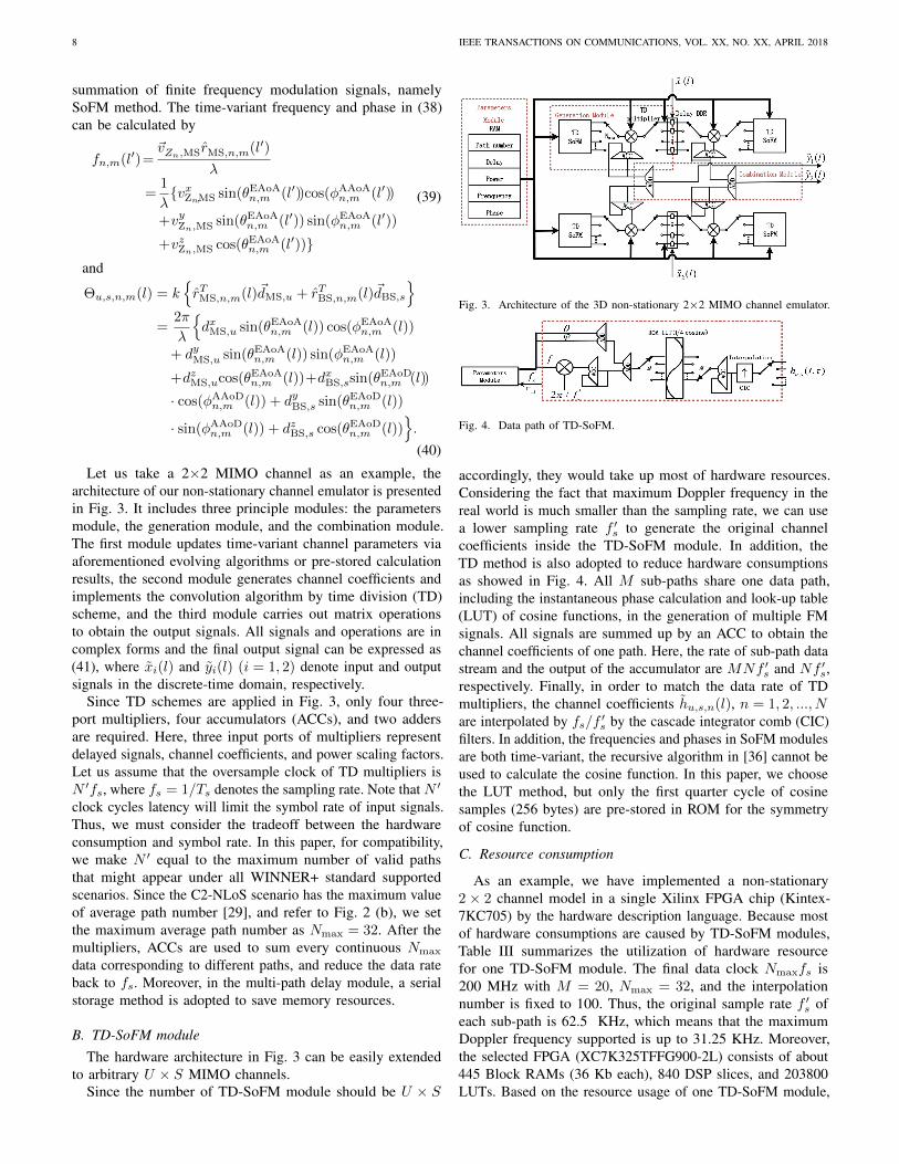
Let us take a 2×2 MIMO channel as an example, thearchitecture of our non-stationary channel emulator is presentedin Fig. 3. It includes three principle modules: the parametersmodule, the generation module, and the combination module.The first module updates time-variant channel parameters viaaforementioned evolving algorithms or pre-stored calculationresults, the second module generates channel coefficients andimplements the convolution algorithm by time division (TD)scheme, and the third module carries out matrix operationsto obtain the output signals. All signals and operations are incomplex forms and the final output signal can be expressed as(41), where xi(l) and yi(l) (i = 1, 2) denote input and outputsignals in the discrete-time domain, respectively.

Since TD schemes are applied in Fig. 3, only four three-port multipliers, four accumulators (ACCs), and two addersare required. Here, three input ports of multipliers representdelayed signals, channel coefficients, and power scaling factors.Let us assume that the oversample clock of TD multipliers isN ′fs, where fs = 1/Ts denotes the sampling rate. Note that N ′

clock cycles latency will limit the symbol rate of input signals.Thus, we must consider the tradeoff between the hardwareconsumption and symbol rate. In this paper, for compatibility,we make N ′ equal to the maximum number of valid pathsthat might appear under all WINNER+ standard supportedscenarios. Since the C2-NLoS scenario has the maximum valueof average path number [29], and refer to Fig. 2 (b), we setthe maximum average path number as Nmax = 32. After themultipliers, ACCs are used to sum every continuous Nmax

data corresponding to different paths, and reduce the data rateback to fs. Moreover, in the multi-path delay module, a serialstorage method is adopted to save memory resources.

B. TD-SoFM moduleThe hardware architecture in Fig. 3 can be easily extended

to arbitrary U × S MIMO channels.Since the number of TD-SoFM module should be U × S

Fig. 3. Architecture of the 3D non-stationary 2×2 MIMO channel emulator.

Fig. 4. Data path of TD-SoFM.

accordingly, they would take up most of hardware resources.Considering the fact that maximum Doppler frequency in thereal world is much smaller than the sampling rate, we can usea lower sampling rate f ′s to generate the original channelcoefficients inside the TD-SoFM module. In addition, theTD method is also adopted to reduce hardware consumptionsas showed in Fig. 4. All M sub-paths share one data path,including the instantaneous phase calculation and look-up table(LUT) of cosine functions, in the generation of multiple FMsignals. All signals are summed up by an ACC to obtain thechannel coefficients of one path. Here, the rate of sub-path datastream and the output of the accumulator are MNf ′s and Nf ′s,respectively. Finally, in order to match the data rate of TDmultipliers, the channel coefficients hu,s,n(l), n = 1, 2, ..., Nare interpolated by fs/f ′s by the cascade integrator comb (CIC)filters. In addition, the frequencies and phases in SoFM modulesare both time-variant, the recursive algorithm in [36] cannot beused to calculate the cosine function. In this paper, we choosethe LUT method, but only the first quarter cycle of cosinesamples (256 bytes) are pre-stored in ROM for the symmetryof cosine function.

C. Resource consumption

As an example, we have implemented a non-stationary2 × 2 channel model in a single Xilinx FPGA chip (Kintex-7KC705) by the hardware description language. Because mostof hardware consumptions are caused by TD-SoFM modules,Table III summarizes the utilization of hardware resourcefor one TD-SoFM module. The final data clock Nmaxfs is200 MHz with M = 20, Nmax = 32, and the interpolationnumber is fixed to 100. Thus, the original sample rate f ′s ofeach sub-path is 62.5 KHz, which means that the maximumDoppler frequency supported is up to 31.25 KHz. Moreover,the selected FPGA (XC7K325TFFG900-2L) consists of about445 Block RAMs (36 Kb each), 840 DSP slices, and 203800LUTs. Based on the resource usage of one TD-SoFM module,


y1(l)

y2(l)

=

N(l)∑n=1

√Pn(ζ)h1,1,n(ζ)x1(ζ−bτn(l)cTs)+

N(l)∑n=1

√Pn(ζ)h1,2,n(ζ)x2(ζ−bτn(l)cTs)

N(l)∑n=1

√Pn(ζ)h2,1,n(ζ)x1(ζ−bτn(l)cTs)+

N(l)∑n=1

√Pn(ζ)h2,2,n(ζ)x2(ζ−bτn(l)cTs)

(41)

TABLE III

HARDWARE RESOURCE USAGE OF TD-SOFM MODULE.

Clock 200 MHz

Channel sample rate 62.5 KHz

DSP∗ slices 16 (1.9%)

LUTs 1524 (0.75%)

Block RAMs∗∗ 17 (3.82%)

Resource utilization 2.16%

*digital signal processing (DSP)

**random-access memory (RAM)

it can also be estimated that a 4×4 MIMO channel with twentymulti-paths for each channel can be emulated on this singlechip.

V. HARDWARE MEASUREMENT RESULTS AND VALIDATION

A. Time-variant Doppler frequency

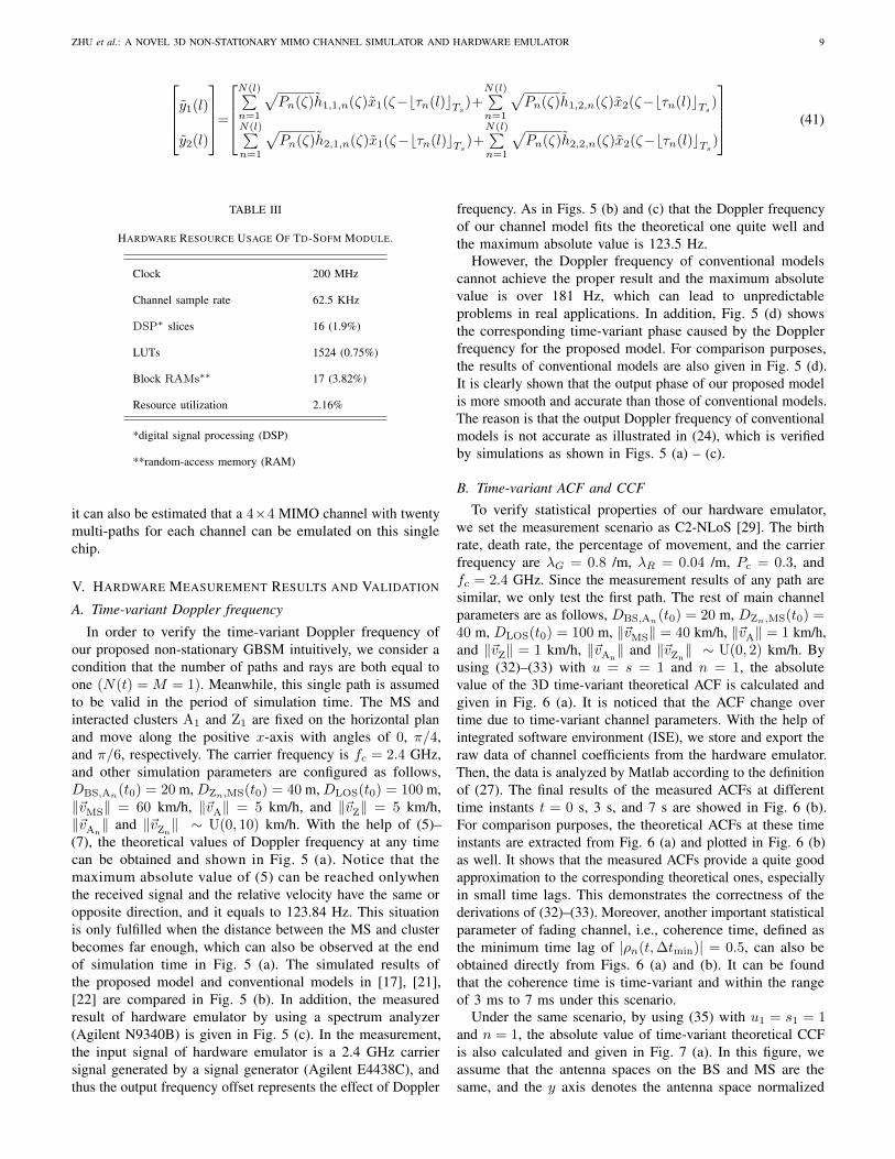
In order to verify the time-variant Doppler frequency ofour proposed non-stationary GBSM intuitively, we consider acondition that the number of paths and rays are both equal toone (N(t) = M = 1). Meanwhile, this single path is assumedto be valid in the period of simulation time. The MS andinteracted clusters A1 and Z1 are fixed on the horizontal planand move along the positive x-axis with angles of 0, π/4,and π/6, respectively. The carrier frequency is fc = 2.4 GHz,and other simulation parameters are configured as follows,DBS,An(t0) = 20 m, DZn,MS(t0) = 40 m, DLOS(t0) = 100 m,‖~vMS‖ = 60 km/h, ‖~vA‖ = 5 km/h, and ‖~vZ‖ = 5 km/h,‖~vAn

‖ and ‖~vZn‖ ∼ U(0, 10) km/h. With the help of (5)–

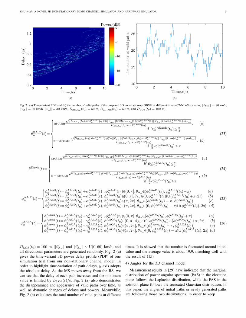
(7), the theoretical values of Doppler frequency at any timecan be obtained and shown in Fig. 5 (a). Notice that themaximum absolute value of (5) can be reached onlywhenthe received signal and the relative velocity have the same oropposite direction, and it equals to 123.84 Hz. This situationis only fulfilled when the distance between the MS and clusterbecomes far enough, which can also be observed at the endof simulation time in Fig. 5 (a). The simulated results ofthe proposed model and conventional models in [17], [21],[22] are compared in Fig. 5 (b). In addition, the measuredresult of hardware emulator by using a spectrum analyzer(Agilent N9340B) is given in Fig. 5 (c). In the measurement,the input signal of hardware emulator is a 2.4 GHz carriersignal generated by a signal generator (Agilent E4438C), andthus the output frequency offset represents the effect of Doppler

frequency. As in Figs. 5 (b) and (c) that the Doppler frequencyof our channel model fits the theoretical one quite well andthe maximum absolute value is 123.5 Hz.

However, the Doppler frequency of conventional modelscannot achieve the proper result and the maximum absolutevalue is over 181 Hz, which can lead to unpredictableproblems in real applications. In addition, Fig. 5 (d) showsthe corresponding time-variant phase caused by the Dopplerfrequency for the proposed model. For comparison purposes,the results of conventional models are also given in Fig. 5 (d).It is clearly shown that the output phase of our proposed modelis more smooth and accurate than those of conventional models.The reason is that the output Doppler frequency of conventionalmodels is not accurate as illustrated in (24), which is verifiedby simulations as shown in Figs. 5 (a) – (c).

B. Time-variant ACF and CCFTo verify statistical properties of our hardware emulator,

we set the measurement scenario as C2-NLoS [29]. The birthrate, death rate, the percentage of movement, and the carrierfrequency are λG = 0.8 /m, λR = 0.04 /m, Pc = 0.3, andfc = 2.4 GHz. Since the measurement results of any path aresimilar, we only test the first path. The rest of main channelparameters are as follows, DBS,An(t0) = 20 m, DZn,MS(t0) =40 m, DLOS(t0) = 100 m, ‖~vMS‖ = 40 km/h, ‖~vA‖ = 1 km/h,and ‖~vZ‖ = 1 km/h, ‖~vAn

‖ and ‖~vZn‖ ∼ U(0, 2) km/h. By

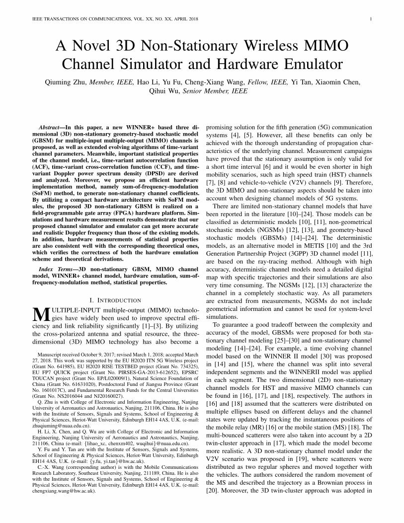
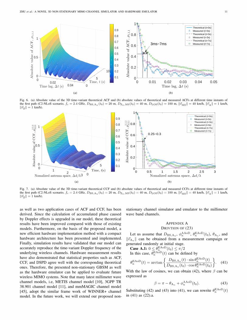
using (32)–(33) with u = s = 1 and n = 1, the absolutevalue of the 3D time-variant theoretical ACF is calculated andgiven in Fig. 6 (a). It is noticed that the ACF change overtime due to time-variant channel parameters. With the help ofintegrated software environment (ISE), we store and export theraw data of channel coefficients from the hardware emulator.Then, the data is analyzed by Matlab according to the definitionof (27). The final results of the measured ACFs at differenttime instants t = 0 s, 3 s, and 7 s are showed in Fig. 6 (b).For comparison purposes, the theoretical ACFs at these timeinstants are extracted from Fig. 6 (a) and plotted in Fig. 6 (b)as well. It shows that the measured ACFs provide a quite goodapproximation to the corresponding theoretical ones, especiallyin small time lags. This demonstrates the correctness of thederivations of (32)–(33). Moreover, another important statisticalparameter of fading channel, i.e., coherence time, defined asthe minimum time lag of |ρn(t,∆tmin)| = 0.5, can also beobtained directly from Figs. 6 (a) and (b). It can be foundthat the coherence time is time-variant and within the rangeof 3 ms to 7 ms under this scenario.

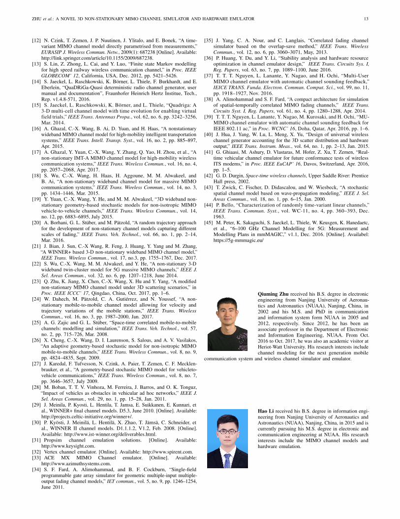
Under the same scenario, by using (35) with u1 = s1 = 1and n = 1, the absolute value of time-variant theoretical CCFis also calculated and given in Fig. 7 (a). In this figure, weassume that the antenna spaces on the BS and MS are thesame, and the y axis denotes the antenna space normalized


-200 -100 0 100 200Doppler frequency, f (Hz)

0

2

4

6

8

10

Tim

e,t(s)

(a)

-200 -100 0 100 200

Doppler frequency, f (Hz)

0

5

10

Time,t(s)

-200 -100 0 100 200

Doppler frequency, f (Hz)

0

5

10

Time,t(s)

(b)

Times,(s)

t

0

2

4

6

8

10

Frequency, (Hz)f2.4 GHz2.39999975GHz 2.40000025GHz

(c)

0 0.1 0.2 0.3 0.4 0.5Time, t(s)

-4

-3

-2

-1

0

1

2

3

4

Phase,ψ

conventional models proposed model Theoretical

(d)

Fig. 5. (a) Theoretical time-variant Doppler frequency, (b) simulated time-variant Doppler frequencies of the proposed model and conventional models [17], [21], [22], (c)measured time-variant Doppler frequency of the proposed model, and (d) simulated phase of the proposed model and conventional models [17], [21], [22] (fc = 2.4 GHz,DBS,An(t0) = 20 m,DZn,MS(t0) = 40 m,DLOS(t0) = 100 m, ‖~vMS‖ = 60 km/h, ‖~vA‖ = 5 km/h, ‖~vZ‖ = 5 km/h).

by the half wavelength. Then, the output CCF of hardwareemulator can be measured by a similar method. Fig. 7 (b)compares the theoretical and measured CCFs at three timeinstants, i.e., t = 0 s, 3 s, and 7 s. From Figs. 7 (a) and(b), we can see that the cross-correlation drops quickly andreaches a relatively low level when the normalized antennaspace beyond 0.5. Since the cross-correlation of the signalsreceived by different antennas will degrade the performance ofMIMO systems, this observation will help us to optimize thelayout of antenna arrays. Again, the well matched theoreticaland measured results validate the correctness of hardwareimplementation, as well as the derivations of (34)–(35).

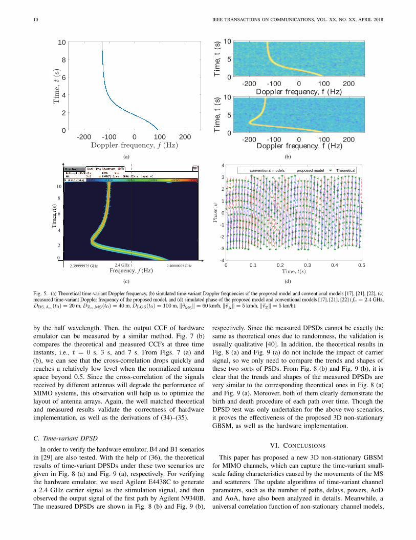
C. Time-variant DPSD

In order to verify the hardware emulator, B4 and B1 scenariosin [29] are also tested. With the help of (36), the theoreticalresults of time-variant DPSDs under these two scenarios aregiven in Fig. 8 (a) and Fig. 9 (a), respectively. For verifyingthe hardware emulator, we used Agilent E4438C to generatea 2.4 GHz carrier signal as the stimulation signal, and thenobserved the output signal of the first path by Agilent N9340B.The measured DPSDs are shown in Fig. 8 (b) and Fig. 9 (b),

respectively. Since the measured DPSDs cannot be exactly thesame as theoretical ones due to randomness, the validation isusually qualitative [40]. In addition, the theoretical results inFig. 8 (a) and Fig. 9 (a) do not include the impact of carriersignal, so we only need to compare the trends and shapes ofthese two sorts of PSDs. From Fig. 8 (b) and Fig. 9 (b), it isclear that the trends and shapes of the measured DPSDs arevery similar to the corresponding theoretical ones in Fig. 8 (a)and Fig. 9 (a). Moreover, both of them clearly demonstrate thebirth and death procedure of each path over time. Though theDPSD test was only undertaken for the above two scenarios,it proves the effectiveness of the proposed 3D non-stationaryGBSM, as well as the hardware implementation.

VI. CONCLUSIONS

This paper has proposed a new 3D non-stationary GBSMfor MIMO channels, which can capture the time-variant small-scale fading characteristics caused by the movements of the MSand scatterers. The update algorithms of time-variant channelparameters, such as the number of paths, delays, powers, AoDand AoA, have also been analyzed in details. Meanwhile, auniversal correlation function of non-stationary channel models,


Time lag, ∆t (s)Time, t (s)

Absolute

valueofACF,ρ1,1,1

10

050

0.5

0.02

1

0.04 0

0.1

0.2

0.3

0.4

0.5

0.6

0.7

0.8

0.9

(a)

0 0.01 0.02 0.03 0.04 0.050

0.2

0.4

0.6

0.8

1

Time lag, ∆t (s)

Absolute

valueofACF,ρ1,1,1

Theoretical (t=0s)Measured (t=0s)Theoretical (t=3s)Measured (t=3s)Theoretical (t=7s)Measured (t=7s)3ms~7ms

(b)

Fig. 6. (a) Absolute value of the 3D time-variant theoretical ACF and (b) absolute values of theoretical and measured ACFs at different time instants ofthe first path (C2-NLoS scenario, fc = 2.4 GHz, DBS,An (t0) = 20 m, DZn,MS(t0) = 40 m, DLOS(t0) = 100 m, ‖~vMS‖ = 40 km/h, ‖~vA‖ = 1 km/h,‖~vZ‖ = 1 km/h).

Time, t(s)

Absolute

valueofCCF,ρ1,1,1

2,2,1

Nomalized antenna space, ∆d/λ

500

0.5

12

1

03

0.1

0.2

0.3

0.4

0.5

0.6

0.7

0.8

0.9

(a)

0 0.5 1 1.5 2 2.5 3Nomalized antenna space, ∆d/λ

0

0.2

0.4

0.6

0.8

1

Absolute

valueofCCF,ρ1,1,1

2,2,1

Theoretical (t=0s)Measured (t=0s)Theoretical (t=3s)Measured (t=3s)Theoretical (t=7s)Measured (t=7s)

0.25~0.3

(b)

Fig. 7. (a) Absolute value of the 3D time-variant theoretical CCF and (b) absolute values of theoretical and measured CCFs at different time instants ofthe first path (C2-NLoS scenario, fc = 2.4 GHz, DBS,An (t0) = 20 m, DZn,MS(t0) = 40 m, DLOS(t0) = 100 m, ‖~vMS‖ = 40 km/h, ‖~vA‖ = 1 km/h,‖~vZ‖ = 1 km/h).

as well as two application cases of ACF and CCF, has beenderived. Since the calculation of accumulated phase causedby Doppler effects is upgraded in our model, these theoreticalresults have been improved compared with those of existingmodels. Furthermore, on the basis of the proposed model, anew efficient hardware implementation method with a compacthardware architecture has been presented and implemented.Finally, simulation results have validated that our model canaccurately reproduce the time-variant Doppler frequency of theunderlying wireless channels. Hardware measurement resultshave also demonstrated that statistical properties such as ACF,CCF, and DSPD agree well with the corresponding theoreticalones. Therefore, the presented non-stationary GBSM as wellas the hardware emulator can be applied to evaluate futurewireless MIMO systems. Note that many latest millimeter wavechannel models, i.e, METIS channel model [10], 3GPP TR38.901 channel model [11], and mmMAGIC channel model[45], adopt the similar frame work of WINNER+ channelmodel. In the future work, we will extend our proposed non-

stationary channel simulator and emulator to the millimeterwave band channels.

APPENDIX ADRIVTION OF (23)

Let us assume that DBS,An , φAAoDn , θEAoD

n (t0), θAn , and‖~vAn‖ can be obtained from a measurement campaign orgenerated randomly at initial stage.

Case A.1: 0 ≤ θEAoDn (t0) ≤ π/2

In this case, θEAoDn (t) can be defined by

θEAoDn (t) = arctan

{DBS,An(t) · sin θEAoD

n (t)

DBS,An(t0) · cos θEAoDn (t0)

}. (41)

With the law of cosines, we can obtain (42), where β can beexpressed as

β = π − θAn + φAAoDn (t0). (43)

Substituting (42) and (43) into (41), we can rewrite θEAoDn (t)

in (41) as (22).a.


(a) (b)

Fig. 8. (a) Theoretical and (b) measured time-variant DPSDs of the first path of the proposed 3D non-stationary GBSM (B4 scenario, fc = 2.4 GHz,DBS,An (t0) = 20 m, DZn,MS(t0) = 40 m, DLOS(t0) = 100 m, ‖~vMS‖ = 60 km/h, ‖~vA‖ = 1 km/h, ‖~vZ‖ = 1 km/h).

(a) (b)

Fig. 9. (a) Theoretical and (b) measured time-variant DPSDs of the first path of the proposed 3D non-stationary GBSM (B1 scenario, fc = 2.4 GHz,DBS,An (t0) = 20 m, DZn,MS(t0) = 40 m, DLOS(t0) = 100 m, ‖~vMS‖ = 60 km/h, ‖~vA‖ = 1 km/h, ‖~vZ‖ = 1 km/h).

DBS,An(t) sin θEAoDn (t)=

√[DBS,An(t0) sin θEAoD

n (t0)]2+‖~vAnt‖2−2·DBS,An(t0)·sin θEAoDn (t0)·‖~vAnt‖·cosβ (42)

Case A.2: π/2 ≤ θEAoDn (t0) ≤ π

In this case, θEAoDn (t) can be defined by

θEAoDn (t)=π−arctan

{DBS,An(t) · sin θEAoD

n (t)

DBS,An(t0) · cos θEAoDn (t0)

}. (44)

Substituting (42) and (43) into (44), we can obtain θEAoDn (t)

as (22).b.

REFERENCES

[1] M. Agiwal, A. Roy, and N. Saxena, “Next generation 5G wireless networks:a comprehensive survey,” IEEE Commun. Surv. & Tutor., vol. 18, no. 3,pp. 1617–1655, Aug. 2016.

[2] C.-X. Wang, S. Wu, L. Bai, X. You, J. Wang, and C. L. I, “Recentadvances and future challenges for massive MIMO channel measurementsand models,” Sci. China Inf. Sci., vol. 59, no. 2, pp. 1–16, Feb. 2016.

[3] C.-X. Wang, F. Haider, X. Gao, X. You, Y. Yang, D. Yuan, et al.,“Cellular architecture and key technologies for 5G wireless communicationnetworks,” IEEE Commun. Mag., vol. 52, no. 2, pp. 122–130, Feb. 2014.

[4] J. Zhang, C. Pan, F. Pei, G. Liu, and X. Cheng, “Three-dimensional fadingchannel models: a survey of elevation angle research,” IEEE Commun.Mag., vol. 52, no. 6, pp. 218–226, June 2014.

[5] M. Shafi, M. Zhang, A. L. Moustakas, P. J. Smith, A. F. Molisch, F.Tufvesson, et al., “Polarized MIMO channels in 3-D: models, measurementsand mutual information,” IEEE J. Sel. Areas Commun., vol. 24, no. 3,pp. 514–527, Mar. 2006.

[6] A. Ispas, G. Ascheid, C. Schneider, and R. S. Thoma, “Analysis of localquasi-stationarity regions in an urban macrocell scenario,” in Proc. IEEEVTC’ 10, Taipei, Taiwan, May 2010, pp. 1–5.

[7] B. Chen, Z. Zhong, and B. Ai, “Stationarity intervals of time-variantchannel in high speed railway scenario,” China Commun., vol. 9, no. 8,pp. 64–70, Aug. 2012.

[8] C.-X. Wang, A. Ghazal, B. Ai, P. Fan, and Y. Liu, “Channel measurementsand models for high-speed train communication systems: a survey,” IEEECommun. Surveys Tuts., vol. 18, no. 2, pp. 974–987, 2nd Quart., 2016.

[9] A. Paier, T. Zemen, L. Bernado, G. Matz, J. Karedal, N. Czink, et al.,“Non-WSSUS vehicular channel characterization in highway and urbanscenarios at 5.2 GHz using the local scattering function,” in Proc. Int.ITG WSA’ 08, Darmstadt, Germany, Feb. 2008, pp. 9–15.

[10] L. Raschkowski, P. Kyosti, K. Kusume, T. Jamsa, V. Nurmela, A.Karttunen, et al., METIS channel models. D1.4 V3, July 2015. [Online].Available: http://www.metis2020.com.

[11] 3GPP TR. 36.873, “Study on 3D channel model for LTE,” V12.2.0,June 2015. [Online]. Available: http://www.3gpp.org/DynaReport/TSG-WG–R1.htm?Itemid=300.


[12] N. Czink, T. Zemen, J. P. Nuutinen, J. Ylitalo, and E. Bonek, “A time-variant MIMO channel model directly parametrised from measurements,”EURASIP J. Wireless Commun. Netw., 2009(1): 687238 [Online]. Available:http://link.springer.com/article/10.1155/2009/687238.

[13] S. Lin, Z. Zhong, L. Cai, and Y. Luo, “Finite state Markov modellingfor high speed railway wireless communication channel,” in Proc. IEEEGLOBECOM’ 12, California, USA, Dec. 2012, pp. 5421–5426.

[14] S. Jaeckel, L. Raschkowski, K. Borner, L. Thiele, F. Burkhardt, and E.Eberlein, “QuaDRiGa-Quasi deterministic radio channel generator, usermanual and documentation”, Fraunhofer Heinrich Hertz Institue, Tech.,Rep. v1.4.8-571, 2016.

[15] S. Jaeckel, L. Raschkowski, K. Borner, and L. Thiele, “Quadriga: A3-D multi-cell channel model with time evolution for enabling virtualfield trials,” IEEE Trans. Antennas Propa., vol. 62, no. 6, pp. 3242–3256,Mar. 2014.

[16] A. Ghazal, C.-X. Wang, B. Ai, D. Yuan, and H. Haas, “A nonstationarywideband MIMO channel model for high-mobility intelligent transportationsystems,” IEEE Trans. Intell. Transp. Syst., vol. 16, no. 2, pp. 885–897,Apr. 2015.

[17] A. Ghazal, Y. Yuan, C.-X. Wang, Y. Zhang, Q. Yao, H. Zhou, et al., “Anon-stationary IMT-A MIMO channel model for high-mobility wirelesscommunication systems,” IEEE Trans. Wireless Commun., vol. 16, no. 4,pp. 2057–2068, Apr. 2017.

[18] S. Wu, C.-X. Wang, H. Haas, H. Aggoune, M. M. Alwakeel, andB. Ai, “A non-stationary wideband channel model for massive MIMOcommunication systems,” IEEE Trans. Wireless Commun., vol. 14, no. 3,pp. 1434–1446, Mar. 2015.

[19] Y. Yuan, C.-X. Wang, Y. He, and M. M. Alwakeel, “3D wideband non-stationary geometry-based stochastic models for non-isotropic MIMOvehicle-to-vehicle channels,” IEEE Trans. Wireless Commun., vol. 14,no. 12, pp. 6883–6895, July 2015.

[20] A. Borhani, G. L. Stuber, and M. Patzold, “A random trajectory approachfor the development of non-stationary channel models capturing differentscales of fading,” IEEE Trans. Veh. Technol., vol. 66, no. 1, pp. 2–14,Mar. 2016.

[21] J. Bian, J. Sun, C.-X Wang, R. Feng, J. Huang, Y. Yang and M. Zhang,“A WINNER+ based 3-D non-stationary wideband MIMO channel model,”IEEE Trans. Wireless Commun., vol. 17, no.3, pp. 1755–1767, Dec. 2017.

[22] S. Wu, C.-X. Wang, M. M. Alwakeel, and Y. He, “A non-stationary 3-Dwideband twin-cluster model for 5G massive MIMO channels,” IEEE J.Sel. Areas Commun., vol. 32, no. 6, pp. 1207–1218, June 2014.

[23] Q. Zhu, K. Jiang, X. Chen, C.-X. Wang, X. Hu and Y. Yang, “A modifiednon-stationary MIMO channel model under 3D scattering scenarios,” inProc. IEEE ICCC’ 17, Qingdao, China, Oct. 2017, pp. 1–6.

[24] W. Dahech, M. Patzold, C. A. Gutierrez, and N. Youssef, “A non-stationary mobile-to-mobile channel model allowing for velocity andtrajectory variations of the mobile stations,” IEEE Trans. WirelessCommun., vol. 16, no. 3, pp. 1987–2000, Jan. 2017.

[25] A. G. Zajic and G. L. Stuber, “Space-time correlated mobile-to-mobilechannels: modelling and simulation,” IEEE Trans. Veh. Technol., vol. 57,no. 2, pp. 715–726, Mar. 2008.

[26] X. Cheng, C.-X. Wang, D. I. Laurenson, S. Salous, and A. V. Vasilakos,“An adaptive geometry-based stochastic model for non-isotropic MIMOmobile-to-mobile channels,” IEEE Trans. Wireless Commun., vol. 8, no. 9,pp. 4824–4835, Sept. 2009.

[27] J. Karedal, F. Tufvesson, N. Czink, A. Paier, T. Zemen, C. F. Mecklen-brauker, et al., “A geometry-based stochastic MIMO model for vehicleto-vehicle communications,” IEEE Trans. Wireless Commun., vol. 8, no. 7,pp. 3646–3657, July 2009.

[28] M. Boban, T. T. V. Vinhoza, M. Ferreira, J. Barros, and O. K. Tonguz,“Impact of vehicles as obstacles in vehicular ad hoc networks,” IEEE J.Sel. Areas Commun., vol. 29, no. 1, pp. 15–28, Jan. 2011.

[29] J. Meinila, P. Kyosti, L. Hentila, T. Jamsa, E. Suikkanen, E. Kunnari, etal., WINNER+ final channel models. D5.3, June 2010. [Online]. Available:http://projects.celtic-initiative.org/winner+/.

[30] P. Kyosti, J. Meinila, L. Hentila, X. Zhao, T. Jamsa, C. Schneider, etal., WINNER II channel models. D1.1.1.2, V1.2, Feb. 2008. [Online].Available: http://www.ist-winner.org/deliverables.html.

[31] Propsim channel emulation solutions. [Online]. Available:http://www.keysight.com.

[32] Vertex channel emulator. [Online]. Available: http://www.spirent.com.[33] ACE MX MIMO Channel emulator. [Online]. Available:

http://www.azimuthsystems.com.[34] S. F. Fard, A. Alimohammad, and B. F. Cockburn, “Single-field

programmable gate array simulator for geometric multiple-input multiple-output fading channel models,” IET commun., vol. 5, no. 9, pp. 1246–1254,June 2011.

[35] J. Yang, C. A. Nour, and C. Langlais, “Correlated fading channelsimulator based on the overlap-save method,” IEEE Trans. WirelessCommun., vol. 12, no. 6, pp. 3060–3071, May, 2013.

[36] P. Huang, Y. Du, and Y. Li, “Stability analysis and hardware resourceoptimization in channel emulator design,” IEEE Trans. Circuits Sys. I,Reg. Papers, vol. 63, no. 7, pp. 1089–1100, June 2016.

[37] T. T. T. Nguyen, L. Lanante, Y. Nagao, and H. Ochi, “Multi-UserMIMO channel emulator with automatic channel sounding feedback,”IEICE TRANS. Funda. Electron. Commun. Comput. Sci., vol. 99, no. 11,pp. 1918–1927, Nov. 2016.

[38] A. Alimohammad and S. F. Fard, “A compact architecture for simulationof spatial-temporally correlated MIMO fading channels,” IEEE Trans.Circuits Syst. I, Reg. Papers, vol. 61, no. 4, pp. 1280–1288, Apr. 2014.

[39] T. T. T. Nguyen, L. Lanante, Y. Nagao, M. Kurosaki, and H. Ochi, “MU-MIMO channel emulator with automatic channel sounding feedback forIEEE 802.11 ac,” in Proc. WCNC’ 16, Doha, Qatar, Apr. 2016, pp. 1–6.

[40] J. Hua, J. Yang, W. Lu, L. Meng, X. Yu, “Design of universal wirelesschannel generator accounting for the 3D scatter distribution and hardwareoutput,” IEEE Trans. Instrum. Meas., vol. 64, no. 1, pp. 2–13, Jan. 2015.

[41] G. Ghiaasi, M. Ashury, D. Vlastaras, M. Hofer, Z. Xu, T. Zemen, “Real-time vehicular channel emulator for future conformance tests of wirelessITS modems,” in Proc. IEEE EuCAP’ 16, Davos, Switzerland, Apr. 2016,pp. 1–5.

[42] G. D. Durgin, Space-time wireless channels, Upper Saddle River: PrenticeHall press, 2002.

[43] T. Zwick, C. Fischer, D. Didascalou, and W. Wiesbeck, “A stochasticspatial channel model based on wave-propagation modeling,” IEEE J. Sel.Areas Commun., vol. 18, no. 1, pp. 6–15, Jan. 2000.

[44] P. Bello, “Characterization of randomly time-variant linear channels,”IEEE Trans. Commun. Syst., vol. WC-11, no. 4, pp. 360–393, Dec.1963.

[45] M. Peter, K. Sakaguchi, S. Jaeckel, L. Thiele, W. Keusgen, K. Hanedaetc,et al., “6–100 GHz Channel Modelling for 5G: Measurement andModelling Plans in mmMAGIC,” v1.1, Dec. 2016. [Online]. Availabel:https://5g-mmmagic.eu/

Qiuming Zhu received his B.S. degree in electronicengineering from Nanjing University of Aeronau-tics and Astronautics (NUAA), Nanjing, China, in2002 and his M.S. and PhD in communicationand information system form NUAA in 2005 and2012, respectively. Since 2012, he has been anassociate professor in the Department of Electronicand Information Engineering, NUAA. From Oct.2016 to Oct. 2017, he was also an academic visitor atHeriot-Watt University. His research interests includechannel modeling for the next generation mobile

communication system and wireless channel simulator and emulator.

Hao Li received his B.S. degree in information engi-neering from Nanjing University of Aeronautics andAstronautics (NUAA), Nanjing, China, in 2015 and iscurrently pursuing his M.S. degree in electronic andcommunication engineering at NUAA. His researchinterests include the MIMO channel models andhardware emulation.


Yu Fu received the BSc degree in Computer Sciencefrom Huaqiao University, Fujian, China, in 2009,the MSc degree in Information Technology (MobileCommunications) from Heriot-Watt University, Ed-inburgh, U.K., in 2010, and the PhD degree in Wire-less Communications from Heriot-Watt University,Edinburgh, U.K., in 2015. He has been a PostdocResearch Associate of Heriot-Watt University since2015. His main research interests include advancedMIMO communication technologies, wireless chan-nel modeling and simulation, RF tests, and software

defined networks.

Cheng-Xiang Wang (S’01-M’05-SM’08-F’17) re-ceived the B.Sc. and M.Eng. degrees in commu-nication and information systems from ShandongUniversity, China, in 1997 and 2000, respectively,and the Ph.D. degree in wireless communicationsfrom Aalborg University, Denmark, in 2004.

He was a Research Assistant with the HamburgUniversity of Technology, Hamburg, Germany, from2000 to 2001, a Research Fellow at the Universityof Agder, Grimstad, Norway, from 2001 to 2005,and a Visiting Researcher with Siemens AG-Mobile

Phones, Munich, Germany, in 2004. He has been with Heriot-Watt University,Edinburgh, U.K., since 2005, and became a Professor in wireless communica-tions in 2011. He is also an Honorary Fellow at The University of Edinburgh,U.K., a Chair Professor of Shandong University, and a Guest Professor ofSoutheast University, China. He has co-authored two books, one book chapter,and over 320 papers in refereed journals and conference proceedings. Hiscurrent research interests include wireless channel measurements/modeling and(B)5G wireless communication networks, including green communications,cognitive radio networks, high mobility communication networks, massiveMIMO, millimeter wave communications, and visible-light communications.

Dr. Wang is a fellow of the IET and HEA. He received nine Best PaperAwards from IEEE GLOBECOM 2010, IEEE ICCT 2011, ITST 2012, IEEEVTC 2013-Spring, IWCMC 2015, IWCMC 2016, IEEE/CIC ICCC 2016, andWPMC 2016. He has served as a technical program committee (TPC) member,the TPC chair, and a general chair for over 80 international conferences. Hehas served as an editor for nine international journals, including the IEEETRANSACTIONS ON WIRELESS COMMUNICATIONS from 2007 to 2009,the IEEE TRANSACTIONS ON VEHICULAR TECHNOLOGY since 2011,and the IEEE TRANSACTIONS ON COMMUNICATIONS since 2015. Hewas the Lead Guest Editor of the IEEE JOURNAL ON SELECTED AREASIN COMMUNICATIONS Special Issue on Vehicular Communications andNetworks. He was also a Guest Editor of the IEEE JOURNAL ON SELECTEDAREAS IN COMMUNICATIONS Special Issue on Spectrum and EnergyEfficient Design of Wireless Communication Networks and Special Issueon Airborne Communication Networks, and a Guest Editor of the IEEETRANSACTIONS ON BIG DATA Special Issue on Wireless Big Data. He isrecognized as a Web of Science 2017 Highly Cited Researcher.

Yi TAN received his MSc degree in Wireless Com-munication from Lund University, Sweden, in 2012.Before and after his MSc studies, he worked inthe industry for a few years related to embeddedsystems, mobile phone antenna, and firmware ofRadio chip. He worked as a Research Assistant inLund University in 2010 and Aalborg University fromSeptember 2014 to June 2015. His main researchinterests include wireless channel modeling andsimulation.

Xiaomin Chen received her B.S. degree in electronicengineering from Nanjing University of Aeronau-tics and Astronautics (NUAA), Nanjing, China, in1997 and her M.S. and PhD in communicationand information system form NUAA in 2001 and2010, respectively. Since 2010, she has been anassociate professor in the Department of Electronicand Information Engineering, NUAA. Her researchinterests include the adaptive techniques for the nextgeneration mobile communication system and MIMOchannel models.

Qihui Wu (SM13) received the B.S. degree incommunications engineering and the M.S. and Ph.D.degrees in communications and information systemsfrom the Institute of Communications Engineering,Nanjing, China, in 1994, 1997, and 2000, respectively.From 2003 to 2005, he was a Postdoctoral ResearchAssociate at Southeast University, Nanjing, China.From 2005 to 2007, he was an Associate Professorwith the College of Communications Engineering,PLA University of Science and Technology, Nanjing,China, where he was a Full Professor from 2008 to

2016. Since May 2016, he has been a Full Professor with the College ofElectronic and Information Engineering, Nanjing University of Aeronauticsand Astronautics. From March 2011 to September 2011, he was an AdvancedVisiting Scholar with Stevens Institute of Technology, Hoboken, NJ, USA.His current research interests include the areas of wireless communicationsand statistical signal processing, with emphasis on system design of softwaredefined radio, cognitive radio, and smart radio.

Documents

IEEE TRANSACTIONS ON COMMUNICATIONS, VOL. XX, NO. XX, … · IEEE TRANSACTIONS ON COMMUNICATIONS, VOL. XX, NO. XX, APRIL 2018 1 A Novel 3D Non-Stationary Wireless MIMO Channel Simulator