Embed Size (px)
Citation preview

ADA!1O 3912 HARVARD UNIV CAMBRIDGE MA AIKEN COMPUTATION LAS F/S 9/2CONTROL-THEORETIC FORMULATION OF OPERATING SYSTEMS RESOURCE MAN--ETC(U)MAY 78 R K JAIN N0O01A TA C 0919
UNCLASSIFIED TR-10-78 ML
I .smhhhmhm loI fllfllfllflfflfflfflfmhhhhhhmhlhmhIuIIIIIIIIIIIhumIIIIIIIIIIIIIIfllfllflEEEIIEEEEEEEEE

28
1111I 15 .4 11111L8
M1 I( ii, % 1 I j 1 I


unclassified
~t r) tt;c.-1. r -2. GOVT A-- NO~ 3. RECiPIL-N S CAT&kL,
4. tIL 11;5. TYPL OF REPORT 6PEP[-,:, '.~
Con r etic Formulation of Operating technical reportS s source Management Policies s. PEKORmiNG OR. APCRT t.;4E..,
7. AUTHO 9. CONTRACT OR GRANT NMZr., s,
Jain, .ra Kumar N00014-76-C-0914
5. PtiFOR iZATtQN NAME AND ADOF;ESS I0. PkOGRAM E-CVLE,.. - 7. ,Harva sity AREA & ORK U.IT NNLWE3
Aiken .ion. LaboratoryCambr . aachusetts 02138
II. C 0 OLL!N tt NAME AND ADDRESS 12. REPORT DATEOffi ce of NafI Research May 1978
800 North Quincy Street 13. NUMSEK OF PA3ESArlington, Virginia 22217 193 pages
14. MONt" OFNG AGLNCy NAME 5 ADDRESS,' dj,:. *ern frt,, Cntrolinj Oiisce) IS. SECURITY CLA S. (of ! ,4 r.;.c--
unclassified'$.DECL&$SIFICATION. -N . "SCHEDULE .. ,
6. STTICUTON STATEM.T (of th R Report)unlimited
Il. DISTRitJ'U iC,4 STATEMENT (of the abstract entered in Block ;0, It djiiefent morom Report)
Vt., '!- t.-4,$NTARY NOTES 1
3 . KEY ('1O1$S (Contns . ,eof s c#c. it no~e..ar, atd Adantity by block nvmbe)
resource management policy page replacementstochastic process binary processCPU scheduling memory demand processpredication problem
20. AUSTVCT (Co t.'Inu. on ,,vere oIf. if ncoeeary and ientif y bp block nLzmben)
n..this thesis we propose the following general control-theoreticapproach to the formulation of resource management policies for operatingsystems.
1. In order to develop a resource management policy, model the corres-ponding program behavior as a stochastic process.
DD jA 7 1473 C;TI. It ',)r I NOV (S IS CDS LETEs'.. 0 102- 314. 601 unclassified
SVCURITY CLASSIFICATION OF THIS POGC !. " ..

unclassified
2. Using identification techniques and empirical data, identifya suitable model structure for the process* and estimatetypical values of model parameters.
3. Based on the model, formulate a prediction strategy for thestochastic process, and hence a resource management policy.
The policy so obtained is dynamic in the sense that it varies the alloca-tion of the system resource to a user job depending upon the recent pastbehavior of the job. It, thus, provides the run time optimization not
possible with the queueing theory approach. Also, notice that theindividuality of the job is fully exploited. The key step in theapproach is the formulation of the stochastic process model in such a waythat the allocation problem reduces to a prediction problem. we exemplifythis approach by formulating control-theoretic policies for CPU schedluingand page replacement. Policies for allocation of other shared resources
(e.g., disks) can be, similarly, formulated.
<I
*The term process is used here exclusively in the control-theoretic
sense of stochastic process. To avoid confusion, the term task is
used to denote computer processes e.g., we say "ready tasks" instead
of "ready processes."
['
?:, ( I
.-.

CONTROL-THEORETIC FORMULATION
OF
OPERATING SYSTEMS RESOURCE M4ANAGEMENT POLICIES
by
Raj endra Kumar Ja .n
TR-1O--78
071c
IS~ ~ ~ Ms araWt
4n a
O'R/'d 411C
been notified that this reportis-
Copyrighted.

CONTROL-THEORETIC FORMULATION
OPEATNG SYSEM RESOURCE jNGMN eLL.LE
A thesis presented
by
Rajendra Kumar Jain
to
The Division of Applied SciencesIn partial fulfillment of the requirements
for the dearce of
Doctor of Philosophyin the subject ofK Applied Mathematics
Harvard UniversityCambridge, Masaachusett s
May 1978
Copyright reserved by the author

Page 2
ACKNOWLEDGMENTS
I would like to express my most sincere gratitude to my friends,
acquaintances, professors, and colleagues who helped me directly or
Indirectly towards the completion of this thesis. Special thanks are
due to the following people.
Professor Ugo Gagliardi introduced me to the problem and served as
my thesis advisor. His able guidance and unflagging enthusiasm have
been a constant source of encouragement. A vital factor in giving this
thesis a practical bent was his first-hand knowledge of the industrial
world. His sound judgment and advice on matters, both technical and
r -n tc.:hn.'cn, :cr.
Professor Y. C. flo acted as a member of ny thesis committec.
Whatever I know about control theory is due to him and his colleaques in
the Decision and Control group at Harvard.
Frofessor Thoma E. Cheatham also acted as a member of my thesis
committee. It is his excellent teaching that attracted me to transfer
to the Computer Science group. He introduced me to Professor Gagliardi
and provided financial support from his research contract during the
transition.
Professor Raman Mehra, now President of Scientific Systems,
Incorporated, brought me to Harvard and provided financial assistance
during my first year here.
App2ovwd fc pniLc torea*m;Ttributon Unlimited
fkw"

Page 3
Umesh Dayal, my friend and colleague, while working on his own
thesis on consistency and integrity conditions for database systems,
found time to check the grammatical, stylistic, and technical
consistency of this thesis.
Charles R. Arnold, my fellow student, supplied data on memory
reference patterns of programs and had many fruitful discussions with
me.
Rajan Suri and Krishna Prasad, my friends and colleagues in the
Decision and Control group, helped me through their critical comments
and insightful suggestions.
IMina Shah helped me in text editing and typing in return for
teaching her COBOL progrpmming.
My mother, brothers, and sisters waited patiently half-way around
the globe for me to finish school. The 75 families of the Jain Center
of Greater Boston provided the requisite social and religious atmosphere
that curdb my homesickness.
0
The work presented in this thesis was supported in part by the
Department of Air Force, Rome Air Development Center under contrActs
F30602-76-C-0001, and F30602-77-C-005, and by the Office of Navnl
Research under contraect rIOOO14-76-C-0914.
Rajendra K. JainCambridqe, MassachusettsMay 19, 1978
M

Page 4
TABLE OF CONTENTS
Page
ACKNOWLEDGEMENTS 2
TABLE OF CONTENTS 4
LIST OF FIGURES 6
LIST OF TABLES 7
SYNOPSIS 8
CHAPTER I: INTRODUCTION 1-11.1 Control-theoretic View of an Operating System 1-21.2 Queueing-theoretic View of an Operating System 1-41.3 Limitations of Queueing Theory 1-61.4 Additional Expectations from Control Theory 1-81.5 Survey of Applications of Control Theory 1-91.6 Principal Contributions and Organization
of the Thesis 1-10
CHAPTER II: A CONTROL-THEORETIC APPROACH TO CPU MANAGEMENT 2-12.1 Problem Statement 2-22.2 Control Theoretic Formulation 2-72.3 Effect of Prediction Errors 2-11
2.3.1 Theorem [Non-deterministic Case] 2-132.3.2 Theorem [Deterministic Case] 2-13
2.4 Data Collection 2-172.5 Data Analysis 2-21
2.5.1 Model Identification 2-222.5.2 Parameter Estimation 2-362.5.3 Choosing a neneral Model 2-45
2.6 Scheduling Algorithm Based on theZeroth Order Model 2-53
2.7 Conclusion 2-56
CHAPTER III: A CONTROL-THEORETIC APPROACH TO MEMORY MANAGEMENT 3-13.1 Problem Statement 3-23.2 Control Theoretic Formulation 3-53.3 Cost Expression 3-83.4 Non-stationarity of the Page Reference Process 3-123.5 ARIMA Model of Page Reference Behavior 3-143.6 Page Reference Prediction Using
the ARIMA(1,1,1) Model 3-223.6.1 Open Loop Predictor 3-223.6.2 Closed Loop Prcdictor 3-21
3.7 ARIMA Page Replacement Algorithm 3-263.8 Special Cases of the ARIMA Algorithm 3-30

Page 5
3.9 Limitations of the Formulation 3-353.10 Conclusion 3-38
CHAPTER IV: BOOLEAN MODELS FOR BINARY PROCESSESWITH APPLICATION TO'MEMORY MANAGEMENT 4-14.1 Introduction 4-24.2 Boolean Functions - Fundamentals 4-7
4.2.1 Definition 4-74.2.2 Definition 4-9
4.3 Development of the Poolean Model 4-114.4 Likelihood Function and Parameter Estimation 4-13
4.4.1 Function Lemma 4-134.4.2 Estimation Theorem 4-14
4.5 Measures of Goodness 4-174.6 Prediction 4-19
4.6.1 Prediction Theorem 4-194.6.2 Total Cost Theorem 4-21
4.7 Tabular Method of Binary Process Prediction 4-234.7.1 Example 4-24
4.8 Generalization to k-ary Variables 4-284.8.1 Model 4-294.8.2 Estimation Theorem 4-304.8.3 Measures of Goodness 4-304.8.4 Prediction Theorem 4-314.8.5 Totil Cost Theorem 4-314.8.6 Tabular Method 4-32
4.9 On Model Order Determination 4-354.9.1 Theorem 4-35
4.10 On Stationarity 4-404.11 Page Replacement Using the Boolean Model 4-42
4.11.1 Theorem 4-434.11.2 Theorem 4-44
4.12 Conclusion 4-47
CHAPTEP V: CONCLUSIONS 5-15.1 Summary of Results 5-25.2 Directions for Future Research 5-4
APPENDIX A: A Primer on ARIMA Models A-I
APPENDIX B: Proofs of Theorems on CPU Scheduling B-I
APPENDIX C: Proofs of Theorems on k-ary Processes C-I
REFERENCES R-1
..
-.- - - - -- - - - -

Page 6
No. Title Page
1.1 Control-theoretic view of an operating system 1-3
1.2 Queueing-theoretic view of an operating system 1-5
2.1 Optimal scheduling of two jobs 2-3
2.2 Round robin scheduling with unit time quantum 2-5
2.3 CPU and I/O demands of a typical program 2-8
2.4 CPU demand modeled as a stochastic process 2-10
2.5 Increase in MFT due to prediction error 2-15
2.6 Data plots of CPU demand processes 2-24
2.7 Autocorrelations of CPU demand processes 2-28
2.8 Partial Autocorrelations of CPU demand processes 2-32
2.9 Output of the parameter estimation program 2-37
3.1 References to a page modeled as a binary stochastic process 3-7
3.2 Wiener filter predictor 3-10
3.3 Autocorrelations of page reference processes 3-15
3.4 ACF and PACF of 1st difference process 3-16
3.5 ACF and PACF for ARMA(1,1) model 3-19
3.6 Block diagram representation of predictors 3-25
3.7 Hardware implementation of ARIMA a]gorithm 3-28
3.8 Special cases of ARIMA(1,1,1) algorithm 3-34
3.9 Information used by various page replacement algorithms 3-36
4.1 Analogy between Wiener predictor and Boolean predictor 4-4
4.2 Determination of Model order n 4-38
-,2-3

Pare 7
LIST EOF TABLES
No. Title Page
2.1 Data Collection Experiment 2-18
2.2 List of CPU Demand Processes Analyzed 2-20
2.3 Inverse Autocorrelations of FRCDO.C11 2-35
2.4 Parametcr Estimation for ARMA(1,1) Model 2-46
2.5 Parameter Estimation for ARMi) Model 2-47
2.6 Parameter Estimation for MA(1) Model 2-48
2.7 Parameter Estimation for AR(2) Model 2-49
2.8 Parameter Estimation for MA(2) Model 2-50
2.9 Comparison of Different Models 2-51
3.1 Costs of memory management 3-9
3.2 Parameter value-, for the ARIMA(1,1,1) model 3-20
3.3 Comparison of ARMA models of 1st difference process 3-21
4.1 Tabular Arrangement for Boolean Model 4-26
4.2 Frequency Distribution for Data of Example 4.7.1 .4-27
4.3 Boolean Predictor for Data of Example 4.8.6.1 4-34
4.4 Calculation of the Total Cost TC(n) for Lower Order Models 4-_39
/.

Page 8
This thesis proposes the application of control theory to the
dynamic optimization of computer systems performance. Until now,
queueing theory has been extensively used in the evaluation and modeling
of computer systems. It is a good design and static analysis tool.
However, it provides little run time guidance. For dynamic (run time)
optimization we need to exploit modern control theoretic techniques such
as state space models, stochastic filtering and estimation, time series
analysis, etc. in this thesis, a general control theoretic approach is
proposed for the formulation of operating systems resource management
policies. The approach is exemplified by formulating policies for CPU
and memory management.
The problem of CPU management is that of deciding which task from
among a set of ready tasks should be run next. The main problem
encountered in the practical implementation of theoretically optimal
algorithms is that the service-time requirements of tasks are unknown.
The proposed solution is to model the CPU demand as a stochastic
process, and to predict the future demands of a job from its past
behavior. Several analytical results concerning the effect of
prediction errors are derived. An empirical study of program behavior
is made to find a suitable predictor. Several different models arc
compared. Finally, it is shown that a zeroth order autoregressive
moving average model is the most appropriate one. Based on this
observation an adaptive scheduling algorithm called "SPRPT" (Shortest
Predicted Remaining Processing Time) is proposed.
I - -e

Page 9
The problem of memory management is also formulated as the problem
of predicting future page references from past program behavior. Using
a zero-one stochastic process model for page references, it is shown
that the process is non-stationary. Empirical analysis is presented to
show that the page reference pattern can be satisfactorily modeled by an
autoregressive integrated moving average model of order 1,1,1. A two
stage exponential predictor is derived for the model. Based on this
predictor a new algorithm called "ARIMA Page Replacement Algorithm" is
proposed. This algorithm is shown to be easy to implement. It is shown
that many conventional page replacement algorithms, including Working
Set, are merely boundary cases of the ARIMA algorithm. The conditions
under which these conventional algorithms are optimal are described.
The limitations of the formulation and possible directions for future
extensions are also discussed.
The ARIMA model does not take into account the fact that a binary
process takes only two values, 0 or 1. This discrepancy is removed by
developing Boolean models for such processes. It is shown that if a
binary process is Markov of a finite known order, it can be modeled as
the output of a Boolean (switching) system driven by a set of binary
white noises. Modeling, estimation, and prediction of the process using
the Boolean model is described. A method is developed for optimal
non-linear prediction under any given non-linear cost criterion. All
the results are then generalized to k-ary processes, i.e., processes
which take integer values between 0 and k-1. Finally, the application
of the model to the problem of memory management is described.

INTRDUCTION
Introduction Page 1-2Control-theoretic view
Conventionally an operating system is defined as the set of
computer program modules which control the allocation and use of
equipment resources such as the central processing unit (CPU), main
memory, secondary storage, IO devices and files (MaD741. These
programs resolve conflicts, attempt to optimize performance, and
interface between the user program and computer resources (hardware and
system software).
1.1 CONTROL-THEORETIC VIEW OF AN OPERUTI&NG S.STEM
For a control theorist, an operating system is a set of
controllers which exercise control over the allocation of some system
resource. The goal of each controller is to optimize system performance
while operating within the constraints of resource availability.
Figure 1.1 shows some of the components of an operating system.
The Controllers are represented by circles. The "load controller"
controls the number of jobs allowed to log in. The job controller (job
scheduler, or high level dispatcher) controls the transfer of jobs from
the "submitted" queue to the "ready" queue. This decision is based upon
the availability of resources like memory, magtapes, etc. The CPU
controller (task dispatcher, or low level scheduler) controls the
allocation of the CPU. It selects a task from the set of ready tasks
and allows it to run. The paging controller (page replacement
algorithm, or memory management algorithm) controls the transfer of
pages from virtual memory (disk or drum) to primary memory, and so on.
- - - -- i

nt roductlocn Pige 1-3
log in Rqet
0Submitted JobLoadI Controller
Control ler Job
uuResponse Scheduler
log out 'Tm
MemoryDeallocation
(Garbagecollec tion)
Termination CU-Ready
Paging IController takCPU or
Controller PaeTaskFaulse Scheduler
WO requests
Fiur 1bControl-terei vCoo n rtntrsyslem
A z
_j4
Fiur 1.1 Coto-tertcve o noeaigsse

Introduction Page 1-4Control-theoretic view
The control components of an operating system are not much
different from those of other systems, except probably, in that they are
non-mechanical. Obviously, there is much that can be gained from
control theory in the design and modeling of these components.
Unfortunately, very little control theory has been used for this purpose
so far. Compared with the highly developed theory ofcontrol systems,
most control algorithms used in operating systems today are "primitive".
1._2QUEUEING-THEORETIC VIEW OF AN OPERATING SYSTEM
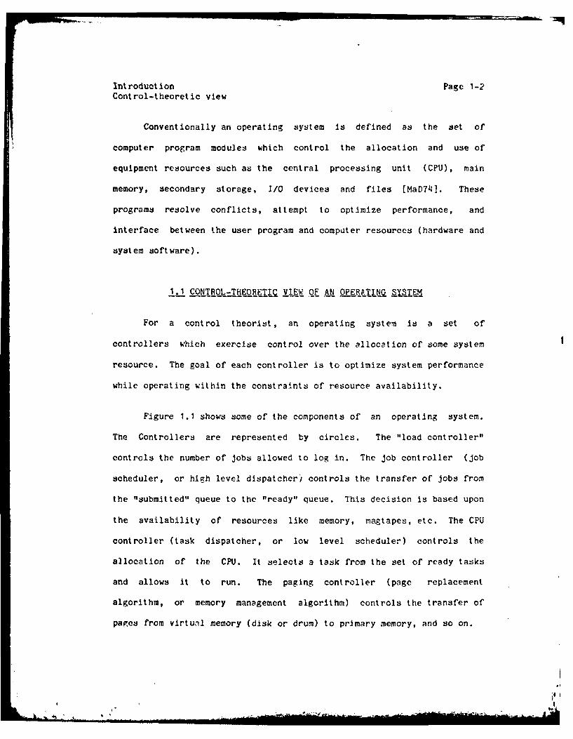
Most models of computer systems used today are queueing-theoretic.
From a queueing-theoretic viewpoint, each controller of the operating
system is a server. Thus, an operating system is a queueing network.
One very popular queueing model, called "Central Server Model", is shown
in Figure 1.2. In this figure, circles represent servers and rectangles
indicate the location of queues. Such queueing models have been used to
explain many phenomena occuring in computer systems [Buz71]. Typical
questions that have been answered using this approach are the
following :
1. What is the average throughput?
2. What is the average utilization of the CPU, I/O devices etc.
3. What is the average response time?
4. What is the bottleneck in the system (would a higher speed disk do
better)?
5. What is the optimal degree of multiprogramming?
_ A _,
Int roduct inn Page 1-5Queue'Ing-theoreti~c view
-------------1------S
eI cI
PoinIDice
ICPU
CETA SEVE
Figur 1. uu n-hoe c iwo no oingsse

Introduction Page 1-6Queueing-theoretic view
A vast amount of literature has been published to answer these and
similar questions under a variety of assumptions, restrictions and
generalizations. For chronological surveys and bibliographies see
[McK69, Mun75, Kle76, LiC77]. Some of the issues investigated are the
following :
I. Service Discipline: M/M/1, G/M/1, MIG/I, FCFS, or priority
service, e.g., see (Shu76].
2. Types of jobs: one or many classes [BCM75).
3. Devices included: Terminals only (Sch67], terminals and I/O
devices [Buz71].
4. State dependent or stationary probabilities (Che75]
5. Exact or approximate solutions [GaS73, Gel75, CHW75]
6. Part by part (hicrarchical) solutions or whole solution [BCE75].
In spite of the wide applications of queueing theory, there are
some inherent limitations to its usefulness.
.L LIMITATIONS OF QU _EG THEORY
Queueing theory represents only average statistics. It tries to
represent a number of jobs by the average characteristics of the class.
The "individuality" of a job is ignored. In this sense, it is a static
analysis. It cannot satisfactorily represent timz varyiij phenomena or
dynamics. Therefore, It is good only as a design time tool. It cannot
be used at operation time, for which we need adaptive techniques that
can adapt to the individual characteristics and time-varying behavior of
,9

Introduction Page 1-7Limitations of queueing theory
Jobs. To give a concrete example, a queueing model is ideal for telling
whether the disk is the bottleneck in the system or whether a faster CPU
will increase efficiency (both design time questions). However, once we
have acquired the proper disk and CPU, it does not tell us which job
from a given a set of jobs should be given the CPU or the disk next.
This is a dynamic decision problem, which can only be solved by the
application of techniques from decision and control theory.
Queueing theory is good for modeling a computer system and, to a
certain extent, its subsystems. However, when we come down to the level
of a program, it cannot model its behavior (because there are no queues
to be modeled). Given all the known information about a program, it
cannot tell what the program behavior is likely to be in the near
future. This is a prediction problem. Again, control theory must be
used for this purpose.
Queueing theory cannot model the interaction between the space and
time demands of a program. Since the theory cannot model either the
space demand behavior of a program or its time demand behavior, it
certainly is inadequate for modeling the interaction between the two.
Bad memory management may cause frequent page faults and may degrade the
performance of an otherwise good scheduling policy. Still, the memory
and the CPU allocation policies of most operating systems to date are
more or less independent. This is due to a lack of clear undcrstandlng
of the interaction between them. With the application of control theory
we hope to remedy this situation, because, riven control-theortio

Introduction Page 1-8Limitations of queueing theory
models of two systems, their joint model can be obtained by modeling the
cross-correlation between the two.
1.4 ADDITIONAL EXPECTATION FOH CONTROL THEORY
There are many concepts like stability, controllability, and
parameter sensitivity, that are well established in control theory but
have not been used in computer systems modeling. We hope that the
control-theoretic approach will eventually lead to a better
understanding of t1se -e concepts as applied to computer systems. For
example, take the oncept of stability. Instability in computer systems
occurs in the for of excessive overhead caused by frequent switching of
CpU between jobs, or by frequent oscillation of pages between main and
secondary memory.. Instability in The control-theoretic approach is
especially suitable for stability studies, e.g., for determining the
effect of sudden demand variations, or the effect of measurement delays.
There are well established techniquec for this purpose.
Controllability studies of computer systems could similarly help
us to determine whether it is possitle to reach the optimum performance
state. Parameter sensitivity is already a big issue even in current
queueing models. One of the major studies that investigated the
applicability of queueing models to a real interactive system was
conducted by Moore at the University of Michigan [Moo71]. One
conclusion of the study was that queueing models are very sensitive to
parameter values which vary considerably with time and load variptions.

Introduction Page 1-9Expectations from control theory
Again, control theory with its well established techniques for
sensitivity analysis provides better hope.
SURVEY OF APPLICATIONS OF CONTROL THEORY
Wilkes was probably the first to strongly advocate the
exploitation of control theory for computer systems modeling. In his
paper [Wil73), he stated:
"We are not yet in a position, end perhaps never willbe, to write down equations of motion for computer systems.However this does not exclude the design of a controlsystem. Indeed, it is just in circumstances where thedynamical equation are not fully understood or when thesystem must operate in an environment that can vary over awide range that control engineering comes into its own."
The paper presents many arpuments for applying control theory. We do
not intend to duplicate those arguments here. To illustrate his ideas,
Wilkes proposed a general model of paging systems.
Adaptive policies for many components of operating systems have
been proposed. Dynamic tuning of allocation policies to improve
throughput in multiproqramming systems has been suggested by Wulf
[Wul69]. An adaptive implementation of a load controller is described
in [WI171 . Blevins and Rampmoorthy have investiqated the feasibility
of a dynamically adaptive operating system [EIR76J. Two different
techniques for adaptive control of the degree of multiprogramming have
been described in [DKL76].

nt roduct ion Page 1-10Literature Survey
The need for a control-theoretic approach was also stressed by
Arnold and Gagliardi [ArG74]. They proposed a state space formulaticn
using resource utilization as the state variables. A dynamic
programming approach to memory management and scheduling problems is
described in [Lew74, Lew76]. A survey of some early applications of
statistical techniques to computer systems analysis can be found in
[Ash72].
The work most closely related to this thesis is that of Arnold
(Arn75, Arn78]. Using correlation properties of the memory demand
behavior of programs, he has investigated the applicability of the
Wiener filter theory to the design of a memory management policy.
1.6 PRINCIPAL CONTRIBUTIONS AND ORGANIZATION OF THE THESIS
In this thesis we propose the following general control-theorctic
approach to the formulation of resource management policies for
operating systems.
1. In order to develop a resource management policy, model the
corresponding program behavior as a stochastic process.
2. Using identification techniques and empirical data, identify a
suitable model structure for the process* and estimate typical
values of model parameters.
* The term process ijs used here exclusively in the control-theoretic
sense of stochastic process. To avoid confusion, the term i' is usedto denote computer processcb e.g., we say "rea.dy tasks" inrite'd of"ready processes".

N iU triLiOtJ, J* .U I. i t
"C LU
Introduction Page 1-11Contributions and organization
3. Based on the model, formulate a prediction strategy for the
stochastic process, and hence a resource management policy.
The policy so obtained is dynamic in the sense that it varies the
allocation of the system resource to a user job depending upon the
recent past behavior of the job. It, thus, provides the run time
optimization not possible with the queueing theory approach. Also,
notice that the individuality of the job is fully exploited. The key
step in the approach is the formulation of the stochastic process model
in such a way that the allocation problem reduces to a prediction
problem. We exemplify this approach by formulating control-theoretic
policies for CPU scheduling and page replacement. Policies for
allocation of other shared resources (e.g., disks) can be, similarly,
formulated.
Formulation of the CPU scheduling policy is described in
Chapter Il. The time taken by successive compute bursts of a program is
modeled as a stochastic process. It is shown that the main problem is
that of predicting the future demands of a job from its past behavior.
A few analytical results are derived concerning the increase in the mean
weighted flow time due to prediction error. Correlation techniques
(also called time series analysis techniques) are used to identify a
suitable model structure for the stochastic process. Empirical data on
the CPU demand behavior of users of an actual time sharing system is
used for this purpose. Details of the procedure used for modeling and
parameter estimation from the data are included. In particular, it is
1.| t ii== in/li a m il'iaibili...

Introduction Page 1-12Contributions and organization
shown that the CPU demand process is a stationary stochastic procss
having very little autocorrelation. The efficiency of several
autoregressive moving average (ARMA) models is compared. The finil
conclusion is that the gains are very small and that a zeroth order
non-zero mean white noise ( ARMA(O,O) ) model is appropriate for the
process. Based on this conclusion, several different predicion schemes
are proposed. An adaptive scheduling algorithm called "Shortest
Predicted Remaining Processing Time" (SPRPT) is proposed.
In Chapter III, the problem of page replacement is formulated as a
prediction problem. Using a stochastic process model of memory demrA
behavior, suggested by Arnold [Arn75], an expression is derived for the
cost of prediction error. The identification analysis shows thct tlw
process is non-stationary. The non-stationarity is, however,
hom%:*neous in the sense that the first differences of the process arc
stationary. An autoregressive integrated movinz average model of order
1,1,1 ( ARIMA(1,1,1) ) is shown to be an appropriate model for the
process. A two step exponential predictor is derived for the model.
Based on this predictor, a new page replacement algorithm called tv.
"ARIMA" algorithm is proposed. Even though the origin of the algcrithi
lies in complex control-theoretic ideas, its final implementation is
very simple. Moreover, it turns out that many conventional page
replacement algorithms like the working set algorithm [Den6], Arnold's
Wiener filter algorithm (Arn75], and the independent reference model
[ADUTI] are special cases of the ARIMA algorithm. The control-theoretir
derivation of the conditions under which these algorithms are optimal

Introduction Page 1-13Contributions and organization
presented.
Chapter IV is devoted to developing new techniques for analysis of
binary processes like the memory demand process. The ARIMA model does
not take into account the fact that a binary process takes only two
values, 0 or 1. In this chapter, an attempt is made to remove this
discrepancy. It is shown that if a binary process is Markov of a finite
known order, it can be modeled as the output of a Boolean (switching)
system driven by a set of binary white noises. Modeling, estimation,
and prediction of the process using the Boolean model is described. A
method is developed for optimal non-linear prediction under any given
linear or non-linear cost criterion. All the results are then
generalized to k-ary processes, i.e., processes which take integer
values between 0 and k-.1 . The model is shown to be applicable to a
class of non-stationary processes also. Finally, the application of the
model to the problem of memory management is described.
In this thesis we make extensive use of control-theoretic terms
and concepts. However, since a mdjority of the readers of the thesis
are likely to be computer scientists, a tutorial approach is followed in
deriving the control-theoretic results. Whenever possible, simple and
intuitive explanations of the infcrences based on control theory are
provided. A brief explanation of ARIMA models, uhich are used
extensively in this thesis, is given in Appendix A. Further details of
control-theoretic concepts can be obtained from [Ne173, BoJ70, Pst7O,
BrH69].
SI tl L ,... 1

CHAPTER jI
A CONTROL THEORETIC APPROACH
IQ-
CPU MANAGEMENT
*1- fl

CPU Management Page 2-2Problem Statement
2.1 PROBLFM STATEMENT
The problem of CPU management is that of deciding which task from
among a set of ready tasks be given the CPU next. In the literature
this problem is also referred to as low level scheduling, short term
scheduling, or process dispatching. There has been a considerable
amount of work on designing scheduling strategies 4 or optimizing
different cost criteria, single or multiprocessor strategies,and for
different precedence constraints among the jobs [Cof76]. A common
underlying assumption in all these researches is that the CPU time
required by each job is known. For example, the simplest scheduling
problem is that of scheduling n independent tasks with known CPU time
requirements of t1, t2, ... Itn respectively on a single processor In such
a way as to minimize average finish time for all users. If the jobs
were scheduled in lexicographic order (i.e., 1,2,...n), the average
finish time would be
R - (n i+l)t i
A very well known solution to this problem is due to
Smith (Sm156]. This solution is called "SPT" or Shortest Processing
Time rule i.e., the jobs are given the CPU ±n the order of
non-decreasing CPU demand For those not familiar with this fact the
following example should prove convincing.
Example : Consider scheduling two jobs J1 and J2 with each requiring
only one cycle of computation followed by output. The time required for
CPU and I/O are shown in Fipure 2.1 . The scheduling decision is to
i7I.

CPU Scheduling Page 2-3
Problem Stt -aecrt
107
1/0J, 0 CPU
15 / 0
J2 6 CPU
A. Job J, is scheduled first. Averoge Response time 17+1 =242 2
Cp0 1
J2CPU
time 0 10 16 17
.. Job J2 is sche.uled first. Averoge Response time 21 2 2222
I/0CPU J2 1 '
time 0 6 16 21 23
Figure 2.1 Optimal scheduling of two jobs
' g'

CPU Management Page 2-4Problem Statement
decide which of the jobs gets the CPU first. Obviously there are only
two options: J1 first, or J2 first. The calculation of the average
response times to the users in the two cases are also shown in the
figure. It is clear that scheduling the shorter job first gives a lower
average response time.
In the case of Line printer scheduling, the service time
requirements can be predicted reasonably accurately from the size of the
file to be printed or by counting the number of linefeeds and formfeeds
if necessary. However, in the case of the CPU, there is no known method
of predicting the future CPU time requirements of the job. This makes
SPT and all similar scheduling strategies unimplementable.
In the absence of knowledge of program behavior, the operating
system designer is left to use his own ad hoc prediction strategy. One
such strategy is to assume that all the tasks are going to take the saxe
(a fixed quantum of) time. The tasks are, therefore, given the CPU in a
round robin fashion for the fixed quantum of time, and if a task has not
completed by the end of the quantum, it is put back on the run queue.
It is obvious that full-information strategies like SPT perform better
than no-information strategies like the fixed-quantum round robin. This
point is illustrated in Figure 2.2 where it is shown that if job J,
happens to be the first in the queue the response time is 25; otherwise,
it is 24.5. In both cases it is more th3n the SPT response time.
i'

CPU Scheduling Page 2-5Problem Statement
A. Round robin with Ji first. Average Response time- 23 + 252 -2
IAO
CPU J J J2I 2 "I J-;1 J J J2 J1 J2 J1 J JI J
time 0 .12 16 23 27
witr~ 23+26B. Round robin with J2 first. Average Response time 2 24 -
22
CPU -J2 J J2 J1 J? J1 , JI J 2 J1 J2 iJ JI. JI JI Jirtime 0 11 16 23 26
Figure 2,2: Round robin scheduling with unit quantum time
, .

CPU Management Page 2-6Problem Statement
Up till now we have assumed that all the tasks arrive
simultaneously and are ready for processing at the same time.
Obviously, this is not the case in a real computer system, where, tasks
arrive intermittently. The optimal scheduling strategy is still
basically the same. At each point in time one makes the best selection
from among those jobs available, considering only the rcmaining
processing time of the job that is currently being executed. This
generalization of SPT is called the Shortest Remaining Processing Time
(SRPT) rule [Smi78]. This minimizes the mean flow time if there is no
extra cost involved in resuming a preempted job. Other results for the
case of simultaneous arrival are similarly applicable. Note, in
particular, that it is not necesjary to have ?ny advance infrmarticn
about job arrivals.
CPU Management Page 2-7Control Theoretic Formulation
2.2 CONTROL THEORETIC FORMULATION
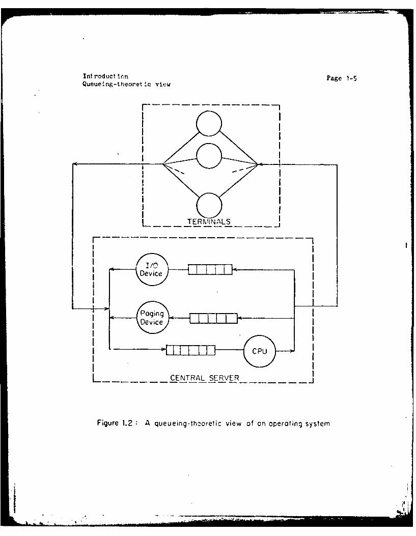
Consider a program in a uniprogramming situation. Figure 2.3
shows the typical time behavior of the program*. The program oscillates
between CPU and I/0 devices (Disk, Teletype, Card reader, Magnetic tape
etc.). Most program have three phases. During the first phase they do
very little computation, spending most of the time collecting parameter
values from the user. The program then enters a computation phase
consisting generally of one or more loops. Finally, the program outputs
the results. The computation phase constitutes a major portion of the
life of the program. The cyclic nature of this phase (due to loops)
makes the program behavior somewhat predictable. While in a loop, the
program repeatedly references the same set of pages, and makes similar
CPU and I/O demands. Under the name of "Principle of Locality", this
behavior has been successfully exploited for memory management. The
working set strategy of memory management is partly based on this
principle. This strategy states that the set of pages referenced during
the last time interval T are more likely to be referenced in the near
future than other pages.
The CPU management equivalent of the WS strategy is to say that
the length of the last CPU burst is the likely length of the next CPU
burst. This strategy has been used in many operating systems, though
there are many different forms of its implementations. One
* The same is applicable to a program in a multiprogramming si uationprovided the time scale represents "virtual time".
* . -.

CPU Schedul~ng Page 2-8Cont rol-theoret ic Formulat ion
Input Phase Computation Phase I Output Phose
1/0
CPU - .......... LI
Figure 2.3: CPU and 1/0 demands of a typical program
...........

CPU Management Page 2-9Control Theoretic Formulation
implementation method is to put a job taking a lot of CPU time on a low
priority queue so that the next time it will get the CPU only afer those
jobs which have taken less CPU time this cycle. Unfortunately, this
principle, although commonly used, hav never been theoretically
explained.
One aim of the research reported here was to check the validity of
this "Next Equal to Last" (NEL) principle, and, if it was found invalid,
to find a strategy for the best prediction of the future CPU demand of a
program from its past behavior. We model the CPU demands of a job as a
stochastic process. The kth CPU burst is modeled as a random variable
z(k). One way of representing a stochastic process is to model it as
the output of a control system driven by white noise (see Figure 2.4).
Thus, as seen by the CPU scheduler, the program is like a control system
which generates successive CPU demands. A general time series model for
such a process is given by the following equation:
z(t) = f(z(1),z(2),...,z(i-1),e(1),e(2),...,e(t))
Where z(t) represents tth CPU burst and e(t) is the tth random shock. A
linearized and time invariant form of the above equation is the well
known ARMA(p,q) model (see Appendix A for details on ARMA models)
z(0) = w+alz(t-1)+ .... +ap z(tp)+e(t).ble(t_1)-...-b qe(tq)
We choose this formulation to model the CPU demand behavior of
programs, because there are well established techniques to find such
models from empirical data. Once a suitable AHMA model is found, it is
easy to convert it to other models (e.g., state space model), if
necessary.
- "-'V . .- -

CPU SchedulinK Page 2-10Control-theoretic Formulat ion
Noise e~t )Linear System CPUDemands z Ct)
Figure 2.4-. CPU demands modeled as a stochastic process

CPU Management Page 2-11Effect of Prediction Errors
La EFFECT OF PREDICTION ERRORS
In order to study the effect of prediction errors, we need to
choose a performance measure. Consider the problem of scheduling n
independent tasks with CPU time requirements of t lt 2, ...,tn
respectively on a single processor. A schedule consists of specifying
the sequence in which the tasks should be given to the processor. There
are many different performance measures for comparing different
schedules. The measure most commonly used for single processor
scheduling is "Mean Weighted Finish Time" (MWFT). It is defined as
follows:
C=1
n wifi
Where fi is the finishing time of ith task and wi is the weight or
deferral cost of the task. It was shown by Smith (Smi563 that this cost
criterion is minimized by arranging the tasks in the order of
non-decreasing ratio ti/wi" If all the tasks have equal deferral costs,
i.e., vi wI :1, then the cost c is called average finishing time or
average response time. It follows from the above that the average
response time is minimized by sequencing the tasks in the order of
non-decreasing ti. This rule is commonly known as "Shortest Processing
Time" (SPT) rule.
It has been shown that SPT also minimizes the following cost
criteria [CMM61]:
1. Mean power of finishing time 1rL fikn i

CPU Management Page 2-12Effect of Prediction Errors
2. Mean waiting time 1 (ftn - t (fi-ti)
3. Mean power of waiting time.
4. Mean lateness (time beyond deadline).
5. Mean tardiness if all jobs are tardy.
6. Mean number of tasks waiting
However, SPT does not optimize the following cost criteria (all of which
are functions of due dates):
1. Maximum lateness
2. Maximum tardiness
3. Mean tardiness
4. Number of tardy jobs.
Fortunately, due dates are rarely, if ever, specified for CPU scheduling
and hence the above criteria are of no practical interest. For a
computer user the most important criterion is a low response time*.
Since a job consists of several CPU-I/O cycles (or CPU-I/O tasks), the
response time is the sum of the finishing time of these tasks of the
job. A" increase in the finishing time of a task directly contributes
to an increase in the response time.
* Some researchers believe that It is the consistency of response timrrather than minimality that is of concern to a user (HoP72. Forexample, If a program takes 1 minute on one day, it Is quite bothersometo the user if it takes 5 minutes on another day. However, the prop'rcontrol point for this criterion is loid control (control cf the nunberof users allowed to log in or the nuTber of batch jobs allowed to rumsimultaneously). Therefore, we do not consider this criterion.

CPU Management Page 2-13Effect of Prediction Errors
In the following, we derive a few analytical results corcerning
the increase in mean weighted finishing time (MWFT) of tasks due to
prediction errors. We first consider a very general case where the time
requirements of all jobs are to be predicted. Then we consider another
case, where only one job is considered for prediction, the compute time
requirements of other jobs is assumed to be known. The results are
presented as Theorems 2.3.1 and 2.3.2 below. The proofs of theorems are
given in Appendix B.
2.3.1 Theorem (Non-deterministic Case] : Consider a set of n tasks T
TI, ..., Tn- with compute time requirements of to, t1l, .. , tn
respectively, where all the times are unknown and are predicted as to,
fl, ..., rn- 1 etc. The predictor is such that the predicted time ti is
a random variable with distribution Fi(ti). The increase in the mean
finishing time (MFT) due to prediction error is given by
n (i-i) tii=O
where 1 Predicted position of T
a)
= f Fj(t)] fi(t)dt
0
..L2 THEOREM [Deterministic Case) Given a set of n tasks
T0,Tl,...,TnI with compute time requirements of to,tl,... ,tn~ 1
respectively, where t ,...,tn1 are known exactly and to is predicted as
tp, then the increase in mean weighted finishing time (MWFT) due to
prediction error is given by:
A!• . l • ,
t.,. . . . . , -, .owa.",

CPU Management Page 2-14Effect of Predictton Errors
C = ( wOtk - wktO)"kel
tk
Where I=fk : --
wk
to( o tplwO) if to<t p
k(tp/wO, to/w O ) if tp>t0
Informally, I is the set of indices of tasks lying between the piedictEd
and the real position of To. J is the interval between to/w0 and tp/w O .
2.3.2.1 corollary : The increase in mean finishing time (wk=1 vk) due
to to predicted as tp is given by
2 - E!tk-tO,
keIwhere I = {k tO<tk<t p or tp<tk<tO }
One implication of this corollary is that only those tasks that
lie in between the predicted and actual position of the task contribute
to the increase in MFT. Thus if the compute time of various tasks are
arranged in increasing order and plotted as shown in the Figure 2.5,
then the increase in MFT is represented by the hatched area. In the
special case, when these compute times are linearly increasing, the
increase in MFT is proportional to square of the prediction error. This
fact is stated by the following corollary whose proof is given in
Appendix B.
2.3.2.2 corollary : If tk=kT, k=1,2,...,n-1 then the increase in NFT
due to t0 predicted as tp is given approximately by:
c )2c ?(to-tp)
F ~ ~ 'E. ea'0 ...
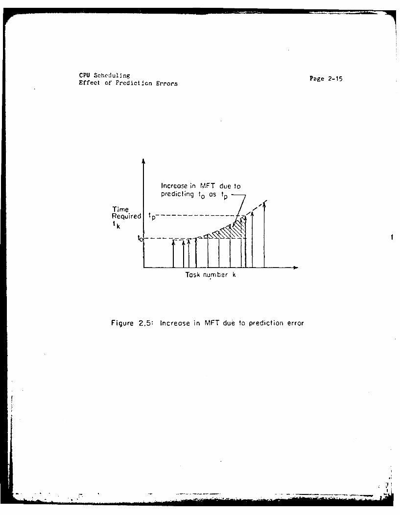
CPU Scheduling Page 2-15Effect of Prediction Errors
Increase in MFT due topredicting to as tp
TimeRequired tp.---------------tk
Task number k
Figure 2.5: Increase in MFT due to prediction error
m ii
CPU Management Page 2-16Effect of Prediction Errors
It is seen from above theorems that the error in prediction of
computer time of a job affects the relative placement of all other jobs
in a very complicated fashion. For example, it is possible that the
time tf... ,tn 1 are far away from one another so that the predicted
value Vi even though away from ti may not result in any change in the
order and hence the net effect on MFT may be zero. On the other hand,
it is also possible that the times t0 1... ,tnl are very near to each
other so that a slight prediction error may result in a substantial
change in the schedule and hence in the MFT. Therefore, except in some
very special cases, e.g., in corollary 2.3.2.2, it is not possible to
express the cost of misprediction as a function of predicion error
alone. That is, there is no one simple "f" such that c~f(t 0 ,tp )
represents the loss function. We, therefore, choose to use the
conventional least square criterion to predict the compute time. In
other words, we seek to predict in such a way that the average value of
square difference between the predicted and the actual value is minimum.
A-.

CPU Management Page 2-17Data Collection
g,. DATA COLLECTION
This section describes the experiment to collect data on CPU
demands of actual programs. The experiment was conducted on a real user
environment in our Aiken Computation Laboratory. The laboratory has a
DECsystem-10 computer with TOPS-1O operating system. The system is
mainly a research facility for use by graduate students.
The TOPS-10 operating system maintains a number of queues among
which the jobs are distributed. For example, there is a queue for jobs
waiting to be run, a queue for jobs waiting for disc I/0, a queue for
jobs waiting for TTY I/O etc. Thus, the easiest way to get the data we
require is to watch the queue history of the program i.e., to note the
queue the job is in and to repeat the observation at every clock tick*.
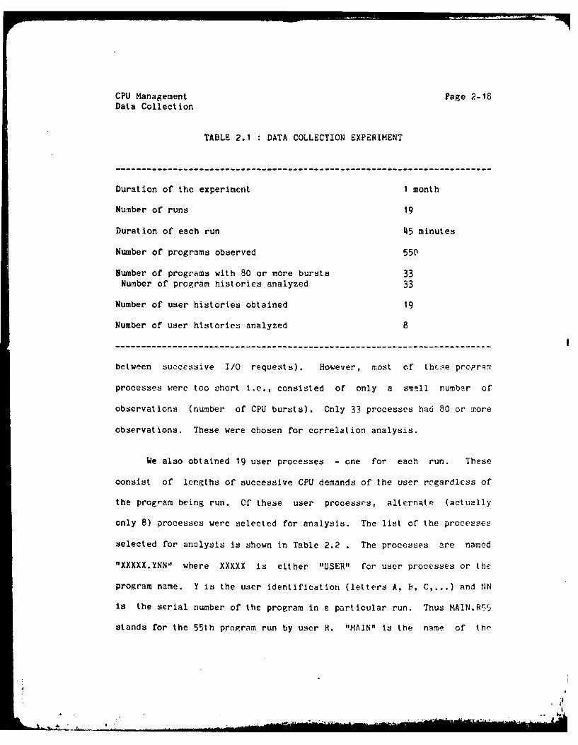
Table 2.1 gives major details of the experiment. It consisted of
19 different runs spread over a month. Each run consisted of randomly
selecting a user and watching his queue history for a period of about 45
minutes. Along with the queue history which was observed every clock
tick, many other parameters like program name, memory used, etc. were
also recorded every second.
The data was later translated to produce the CPU demand processes
of individual programs. This produced 550 CPU dcmand processes
consisting of the length of successive CPU bursts (total CPU usage
.--.-- ...--------------.--..---..... ---- -- -- --.- .--. .---...-- .--..-- . ---
* In all subsequent discussions, the unit of time will be a clock tickcalled "Jiffy" in DISC terminology. A jiffy is the cycle period of theline power supply i.e., 1/60th of a eecond.
I4 ,o .
CPU Management Page 2-18Data Collection
TABLE 2.1 : DATA COLLECTION EXPERIMENT
Duration of the experiment I month
Number of runs 19
Duration of each run 45 minutes
Number of programs observed 550
Number of programs with 80 or more bursts 33Number of program histories analyzed 33
Number of user histories obtained 19
Number of user histories analyzed 8
between successive I/O requests). However, most of thr-e proirami
processes were too short i.e., consisted of only a small number of
observations (number of CPU bursts). Only 33 processes had 80 or more
observations. These were chosen for correlation analysis.
We also obtained 19 user processes - one for each run. These
consist of lengths of successive CPU demands of the user regardless of
the program being run. Of these user processes, alternate (actually
only 8) processes were selected for analysis. The list of the processes
selected for analysis is shown in Table 2.2 . The processes are named
"XXXXX.YNN' where XXXXX is either "USER" for user processes or the
program name. Y is the user identification (letters A, B, C,...) and N
is the serial number of the program in a particular run. Thus MAIN.R55
stands for the 55th program run by user R. "MAIN" is the name of thn
5 5
CPU Management Page 2-19Data Collection
program. Table 2.2 also gives the type of the program, number of
observations in the process, its mean value, standard deviation sz, and
P-VALUE. The term P-VALUE will be explained later under the Chi-square
test.
The developmental nature of the environment is obvious from the
table. Notice that 14 (42%) of the programs are editing (SOS and TECO),
7 (21%) are FORTRAN programs, and 4 (12%) are ELI programs. FORTRAN and
ELI are the main languages used at our laboratory. Most users follow a
cycle of editing (TECO), compiling (FORTR), and running the program, and
then reediting etc. This is typical of research and development
environments. In a production environment in an industry, less amount
of editing and more application program execution is expected. However,
as we shall see later, the CPU demand behavior of editing programs and
application programs are not very different except that the mean value
of CPU burst in an editing program tends to be much lower than that in
an application program. Therefore, it is plausible that the results
obtained here also hold in a production environment.
A I

CPU Management Page 2-20
Data Analysis
Table 2.2 List of CPU Demand Processes Analyzed
S. No. Process N z sz P-VALUE ProgravnName Chi-Sq Type
1. COMP2.G63 158 24.8 85.0 0.000 FORTRAN Provram2. ECL.B1 81 11.2 18.q 0.241 ELI Prcgrm3. ECL.B2 260 74.7 379.9 0.006 ELI Program4. ECL.S1 448 49.0 306.9 0.997 ELI Program5. ECL.S2 270 77.6 528.5 0.999 ELI Propram6. FORTR.P21 113 5.4 7.8 0,178 FORTWAN c rpiIcr
7. FORTR.P30 234 6.3 7.6 0.412 FOR'IRAN compilkr8. FORTH.P8 349 6.2 6.7 0.000 FORTRAN compiler9. FORTR.Q17 253 5.2 6.1 0.001 FORTRAN comnilkr
10. FRCDO.CI 141 606.7 1298.0 0.047 FORTRAN Prok'ran11. FHCDO.CII 158 184.2 578.8 0.003 FORTRAN Pro-tram12. M786S.UI 504 1.5 5.7 0.000 FORTRAN Provram13. MAIN.QIO 204 8.4 7.4 0.000 FORTRAN Prozrar14. MAIN.019 98 8.2 5.9 0.000 FORTRAN Proqram15. MAIN.R55 129 3.4 3.4 0.230 FORTRAN Prozram16. P.A19 222 9.2 23.4 0.000 FORTRAN Prozram,17. PIP.G18 140 1.1 0.7 0.088 Peripherpl I/C16. PIP.G45 84 1.0 0.8 0.000 Peripheral I/C19. PIP.G60 225 0.9 0.3 0.000 Peripheral /C j20. SOS.A21 422 1.9 2.7 0.000 Text Editor21. SOS.A22 85 2.0 2.7 0.6416 Text Editor22. SOS.A23 103 1.5 1.3 0.374 Tcxt Editor23. SOS.A6 110 2.8 3.1 0.606 Text Editor24. 7ECO.B8 90 3.7 6.6 0.916 Text Editor25. TECO.F1 92 2.7 4.6 0.540 TExt Editor26. TECO.F20 199 5.7 6.3 0.018 Text Editor27. TECO.G37 116 28.0 t22.2 0.272 Text Editor28. TECO.G38 221 17.2 64.8 0.140 Text Editor29. TECO.055 114 4.3 4.5 0.000 Text Editor30. TECO.HI 168 2.2 2.8 0,001 Text Editor31. TECO.J5 90 6,4 6.4 0.s74 Text Editor32. TECO.PI 138 4.6 12.6 0.979 Tcxt Editor33. TECO.P13 84 4.3 5.5 0.568 Text Editor34. USER.B 587 37.0 257.7 0.00035. USER.D 259 52.0 329.2 1.00036. USER.F 680 5.5 17.5 1.00037. USER. H 413 6.5 39.9 1.00038. USER.L 372 4.2 7.8 0.00039. USER.N 471 30.2 187.5 0.99940. USER.P 1629 7.1 17.5 0.00041. USER.T 262 25.1 112.0 0.554--------------------------------------------------------------------
.-. .I

CPU Management Page 2-21Data Analysis
Z,5 DATA ANALXSLI
The aim of data analysis is to find one suitable model structure
for CPU demand behavior of programs. The two main steps of data
analysis are model identification and parameter estimation. The first
step consists of studying the first and the second order statistics of
the data in order to identify a class of models suitable for the
process. In the second step, these models are fitted to each process to
find the maximum achievable gain. Finally, these different models are
compared to give one general model for all CPU demand processes. A
large part of the data analysis reported here was done on a time series
analysis package TS developed by Professor Vandalae of Harvard Business
School.
Statistical techniques are very often misused and results
misinterpreted. It is easy to driw misleadinF conclusions unless the
statistical procedures are fully understood and used properly. for
example, we have noticed that in most of the computer science
literature, correlation techniques are used without significance tests,
parameters estimated without their confidence intervals, and so on. We,
therefore, decided to explain the methodology along with the results.
In the following we have tried to describe the reasoning behind each
inference that we draw. The description is, however, brief due to space
limitations and references are provided for further details whenever
necessary.

CPU Management Page 2-22Data Analysis
2,5, 1 Model U~I:[ ,_ta
Model identification consists of studying the characteristic
behavior of the first and the second order statistics of the data. The
goal of this step is to identify a model structure or a class of models
suitable for the data. Notice that this does not include finding an
exact model equation; that is part of the next step on parameter
estimation. The statistics used for model identification in this
analysis are data plots, autocorrelations, partial autocorrelations,
inverse autocorrelations, and Chi square test. The inferences drawn
from these statistics are now described.
2 . .1I Data Plot:
The very first step in any identification procedure must be to plot the
data and to study its general time behavior. The plots of CPU demands
of some of the programs analyzed are shown in Figure 2.6 . These are
typical of all the programs analyzed. Very often a program has just one
or two large CPU bursts which if plotted would obscure the details at
lower values. Therefore, the Y-axis scales have been so chosen that at
least 95% of the data are shown in the graph. Very large value are
shown cut off at the largest plottable value. Notice the following
characteristic behavior of thee araphs:
A. No Trend : A trend (monotonous increase or decrease) in the data is
an indication of non-stationarity, though its absence does not confirm
stationarity. For a stationary series, the mean of the data does not
depend upon time; it is constant. Therrfore, such a series takes trips
lt

CPU Sch, duLng Page 2-23Dnita Analny.
CPU IEIA) [IEHAVICIR .)F ECL S-2 CPU DEM'AND IDLHAVIOR OF '!, ()-10
0 o 7M W . ftM . f . ft *L . N. 0 .Vr fl-TKLJ I=.9 IIII SJMYS. OEM 9. g9 r" , P&I 34.0. C. "-. :~ I N.0
C! 0
NN
Riii00
C; 0
9 C!0N
ri 0 1 (
2COo X 1 11) 2- 0 0 43 E1 I '1i to 240BL RST N'S5E E L3E3E-
CPUJ DEM. E O-AVF-,Q ; C-1 CPU EEkVIr Z 10
0! *41 &POTS. M. 4072 . PN '% 7.l.0 . .. T2.L 234 .p;TS. MEA -AM -. ~ i C.,~ .' * 22.0
8 C!
Lp0
0I
L '40 0 1. 11 &0~ 700 240 0 40 1U .1O eij 2-0
F~gui'cl 2. 6 a- : nit plots~ of CI dvinidc p r c r.-isca
'9 I

CPU Echeduling Page 2-24
Data Analy..
CPU D)EMA BEAVIOR OF PIP G-18 CPU DEMAN~D BLHAVIOfR CF !%CC- -2)
04 ~ ~ 1 BJ10 er* "t 1.2 5 .0 .9 o.'rct:L - 2.0 "V uam'$ .* 2 M.O* )2. FWM.J 20.0
cy Y
0 0
C C!
LiiiNN
ILII It Ur
00.
; '40 90 12) 16) 200 240 0 '40 W) 20 -0
B3LFST NE' BR~NU-
CPU DEHANO -EA\, ICR 09- USEIR 6 CPU DEYAND S-AI~C .-
UPUfk^J. PC- * 3 ..~3O~PAl . 13 SS. IFA - 7.9 . --. . .S
0C0
u 'rbo 1 4 UJ I i*.' I1 ! :.
00wu ;A Lu6 (1 160 '40I 1 : 4:
EAJ' STLU'i NIV'IEFiur 2.b Dt ltso P can rcnw
CPU Management Page 2-25Data Aralyis
away from the mean, but it returns repeatedly during its history.
F.rtunately, none of the CPU demand processes show a trend. Thus we can
hope for stationarity. A more conclusive test of stationarity via the
autocorrelation function will be described in the next section.
B. Violent Variations : Notice that the series does not stay at any
one level even for short intervals. This indicates that a WS-type
prediction scheme (i(t+1)=z(t), i.e., the current CPU burst size is a
good estimate of the next one) is probably not very valid. We may have
to use some more sophisticated scheme.
2...2 Autocorrelation Function :
As the n~me implies, the autocorrelation function is a measure of the
correlation between the present and the past observations. It is
therefore, also a measure of the predictability of future from the paet.
Mathematically, the autocorrelation function is the normalized
autocovariance function. The latter is defined as follows:
Cov(k) = E[(z(t)-z)(z(t+k)-Z)]
By dividing the autocovariance function by the variance (Cov(O)) wZ get
the autocorrelation function C(k):
C(k) = Cov(k)/Cov(O)
Obviously, to be of any value, a stcchastic process should have
finite memory, i.e., the present observation must be correlated only
with those in the finite past. In other words, the autocorrelation
function should die down to zero at very large laps. Such processes arr
called stationary because after a while they achieve "equilibrium" and
.4

CPU Management Page 2-26
Data Analysis
their behavior does not depend upon initial conditions (long past).
Autocorrelation functions (ACF) of some of the CPU demand
processes are shown in Figure 2.7 . These are typical of all the
programs analyzed. The dashed lines indicate the 95% confidence
interval of the ACF for the given sample. The expression given above
for C(k) is valid only for infinite sample sizes. For finite sample
sizes the calculated values are only an approximation tD the theoretical
ACF. Thus if r(k) denotes the standard deviation of C(k), then a
calculated value for theoretically zero autocorrelation (C(k)=O) may lie
anywhere between O.1.98r(k) with 95% probability. In simple words, nny
value between the dotted lines can be effectively assumed to be zero
with 95% confidence. The variance r(k) can be calculated by Bartlett's
formula [Bar46]. In computer science literature, this significance test
is almost always omitted, resulting in misleading conclusions.
The characteristic features of the ACF and the inference that we
can draw are now described.
A. The ACF dies down to zero very auickly. This indicates that the CPU
demand process is stationary. If the ACF had not died down quickly, we
would have had to analyze the ACF of the first and higher differences of
the process.
B. The ACF is non-zyro only for I or 2 lg. We can, therefore,
restrict our consideration to VIA models of order less than 2.
-- -'"-

,CPU Schodul~ng Page 2-27Data Ani.ly.C::
C f 'U D E "r,' No J v ,? F E (.L S 2 C PU C L rA.. r : -. 'o 0," t ,A I,
'0 '00
7. 2',MA- r'6.VD L. S oWll c . 1.01
Z) L... -0 .. .
lk-I-
0
SL0.
0 : v --- -
L ,
CPU D IAND )- A'V-,: 0 -o .Rc0 C-: I Cpu FD,-A,,NC ,",'or AV O Ca FO -7 " = -__
0 0.
F'- C;6 81
b1b
0 0
0 0
6 !Y
0.
16-
C!C
Ngur 28aAI'.re-i n rCUdmndpo:nf:

CPU Schedulng Page 2-28Data Arnly2,3
CPU DECIIA .' LFAVIVC,' CF P P 5-4 CPU CEr1"; EJ-t./ IR CiO TECO 1-211
"0
o 0
.0. 0
<4 04 16 0 6 8 1
2, LGx7 LAG
I- o I- 0
0 - ----------------------------- -- 0
6 6
C P U D E N A % D E - H A V I C ,R U S EE" 9 . .' - C P U D E N N D H W - A V : C . -. . r L IS 7 : - -,Z
z
LL 0 LLQo o
6 2 8 10 1'- 14 16 'C 2 4 6 8 10 1
" J , I-)
-J,---------- - ------C ------- ---- ----------
Ld G
00
0 0
0[0
| . . . . .~ A * ( .~ , i . 4i 'M S LN * L ". A - I " l'C'C
Fleure?.7 o CV d-an prcomwo

CPU Management Page 2-29Data Analysis
It is very important to remember that the sample autocorrelations
are only estimates of the actual autocorrelations for the process which
generated the data at hand. Therefore, the analyst must be on the look
out for general characteristics which are recognizable in the sample
correlogram and not automatically attach significance to every detail.
For example, there is a 5% probability that a theoretically zero
correlation will show up as significant (above the dashed lines).
Therefore, one or two significant correlations at large lags in some of
the cases shown should not alarm us.
C. The ACF is positive. A positive correlation between successive
values indicates that a large CPU demand in one cycle implies a large
demand in the next cycle. Therefore, a program that took a long CPU
time during last cycle can be expected to be CPU bound at least for the
next cycle and put on a lower priority queue.
D. The value of ACF is rather small. The ACF at lower lag values even
though non-zero and positive is really very small (of the order of 0.1).
This partially dulls the hope expressed in the last inference. The
correlation being small, the gain in the predictability of the future
from the past will be small. In nontrol theoretic terms, we are,
perhaps, headed for a zeroth order model.
2I." a& Part ial Auo m~-I Funl,9.0
The PACF is the dual of the ACF. Like the ACF gives an idea of the
order of the MA models, PACF gives an idea of the order of AR models.
If the process is modeled by an AR model of order p:
z(t) w + alz(t-1) + a2 z(t-2) + ... + apz(t-p) + e(t)
*... --..

CPU Management Page 2-30Data Analysis
Then theOcoefficient ap of the last AR term z(t-p) is defined as the
value of PACF at lag p. Naturally, if the real process generating the
data had an AR model of order n, then we would expect PACF to be zero at
all lags greater than n. Thus the cut-off point of the PACF gives the
order of' AR model.
The PACFs of some of the CPU demand processes are shown in
Figure 2.8 . The dashed lines indicate the 95% confidence interval for
the PACF for given sample sizes. It was shown by Quenouille [Que49]
that the approximate standard error of the PACF is n-0 .5 . The
characteristic attributes of these PACFs and their implications are now
described.
A. The PACF dies down to zero very quickly. In fact in most cases the
PACF is significant (above the dashed lines) only for lags 1 or 2. This
means that we do not have to bother about very high order AR models to
model these processes. A first or second order model will do.
B. The PACF is positive at low lags. Notice that the PACF for almost
all processes is positive at lag 1. Only in 1 or 2 cases is PACF(1)
negative. The positive value implies that a CPU bursts gives a pot:itive
contribution to thc estimate of the next burst. It therefore confirms
our previous conclusion that a large CPU burst is more likely to be
followed by another large burst.
L... Chi Saar ic j RnLoq[
One way of viewing the process of modeling a time series is as an
attempt to find a transformation that reduces the observed data to
. . . . - : .. . . :. .. .. . . . -7LA

CPU Schcdul-ng Page 2-317 Data tAnil y:,,.
CPU r.1.flN ..LHAVI C. lZ S-2 CPU DEMAND (,)AVtQ F M!AIN G 10
Mr-B WWIts. Pi - M. . SID. COC. IS.S to4 sIk",. Pmm *IS . ST. cv. .
* 0
o 70
00
- g -- --- --------------- ----- -- ---- --- --- -------- -- ,- ,- ----- ----- --- ---,'..
I-4
LlC
S160.-.--.-.-.-.-.-.---------------........ ........- --------- 8
o C;
f.-f.
J, .
jco
,i z:j .
0-s0
L
z0 c; 4 tz\ " -
000
.o 0" 0
0 0J
Fier 6.8a12< 14 16ria Auor e~n 2£ 4P Io. n 16e'J
0 6.I
J 00
0
AL~ - O Y 1
F~gue 28a artll Atoorreat~cis f CU doandproise

CPU S&hrdullng Page 2-32Data Analy:3.'s
CPU [6rWAND FEh IAV.P (, F PIP 4 - 4 PU ,. .... io 0
04 lS LP1. ra 1.0 1. 10. mv. * o.1 L a*I , V. * MA i ILO l ay. * i
Oo O0
'0 .0
c;.
iCC
ZNI-- -. --------
C 2 14 16 C1 2 4 6
< , <,o<4. <1.
L
CPU ¢.c"D.D5CL EN, cHVC -S<0 <0
0 0
o 0
CPU r~)El.,ND -. ' , "& C, R L'P BCUD .~~2HA1~0 2
o 0o
0; .. . . . .01 2 1 6 t 0 - '
00 0
Oo . O
J0
-100 B20
1-------------------------------------------.. .-------------------------- -------------
* Li . . :
LAG-
n-, n.,<u ' <
c; 4 0
9 9;
Figure 2.8b Pairti~al Autocorr1'it.oti of' CPU di-nip'a~

CPU Management Page 2-33Data Analysis
random noise. The first question, therefore, is whether the data itself
is a random noise. Theoretically, the autocorrelation of random noise
will be zero at all lags. In practice, it will have small non-zero
values. Bartlett's formula for the standard error of the ACF provides
some guidance to test the smallness. A better quantitative test of
randomness is due to Box and Pierce (BoP7O]. They have suggested a
statistic that offers a test of the smallness of a whole set of sample
autocorrelations for lags I through k. This is the Q statistic given by
Q = N c(j)2
Q is approximately Chi-square distributed with k degrees of freedom.
Using the Q statistic one can calculate the probability that the given
sample came from a white noise process. This probability is listed in
the Table 2.2 under P-VALUE. Notice that 22 of the 33 processes
analyzed have non-zero P-VALUE, 16 have P-VALUE greater than 10%, and 8
have P-VALUE greater than 50%. Of the 8 user processes analyzed 4 have
a P-VALUE of 1, i.e., they are almost surely random noises. The high
randomness of the user processes is a result of their being mixtures of
severa] program traces, many of which have no relation to one another.
2..15 jvser.a Autogq.l atg Function
The inverse autosorrelations of a time series are defined to be the
autocorrelations associated with the inverse of the spectral density of
the series, i.e.,
IACF = Inv. Fourier Transform [ 1Fourier Transfrm ACF)3
The IACFs were first proposed by Cleveland [Cle72]. He claims that they
, , - • 4?

CPU Management Page 2-34Data Analysis
are useful in identifying non-zero coefficients in an ARMA model.
However, their utility in model identification is still a point of
debate among statisticians [Par72]. We calculated the inverse
autocorrelation functions for all of our CPU demand data processes.
However, in most cases these functions did not give much additicnal
information. Only in some (2 or 3) cases, where the processes behaved
abnormally (a low order ARMA model was not adequate), did we gain some
insight into modeling these particular cases.
In order to illustrate the use of IACF, let us consider one such
case : the CPU demand behavior of program FRCDO.C11 . Its ACF and PACF
were insignificAnt everywhere except at lags 5, 6, and 14. Obviously, a
low order ARMA model would not work for this process. As we will see in
the next section of wodel fitting, that an AR(2) model resulted in only
1.6% improvement over a zeroth order model. The inverse autccorrelation
for this process (assuraing orders of I through 8 for the AR part of the
model) are shown in Table 2.3 . Notice that all columns except 5 and 6
are zero. Cleveland suggests that this indicates an appropriate model
would have a 6th order AR part with only 5th and 6th coefficients
non-zero and all other coefficient zero, i.e., a model of the follcwing
type :
z(t) = w + a5 z(t_5) + a6z(t-6) + e(t)
Obviously, these high order models are of no interest to us
because of their applicability only in rare cases, and also because of
the rather small rain even in these cases.
dim"I

CPU Management Page 2-35Data Analysis
Table 2.3 : Inverse Autocorrelations of FRCDO.C11
m ri(1) ri(2) ri(3) ri(4) ri(5) ri(6) ri(7) ri(8)
1 -0.076
2 -0.091 0.100
3 -0.074 0.087 0.080
4 -0.072 0.090 0.077 0.014
5 -0.078 0.066 0.046 0.038 -0.162
6 -0.011 0.062 0.026 0.001 -0.135 -0.189
7 -0.018 0.056 0.027 0.003 -0.132 -0.190 0.016
8 -0.019 0.095 0.052 -0.003 -0.140 -0.205 0.026 -0.107
ri(n) = nth inverse autocorrelation
m Order of the AR model used for calculating ri.

CPU Management Page 2-36Data Analysis
2.5.2 L Estimj~jat
In order to find one general model for all CPU demand processes we
fitted several models to each process, and found the best parameter
estimates and hence the maximum improvement available. The details of
the model fitting procedure and the results obtained are the topic of
this section.
The net conclusion of the identification step discussed in the
last section are the following
1. The CPU demand process is a stationary process.
2. The order of the ABMA model required to model the process i
rather small - of the order of 1 or 2.
We, the-efore, limited our search for thm bcst model to the cla5s
of ARMA(p,q) models with p~q < 2. This clpss includes the follovinc s4x
models.
1. 0 0 White Noise z(t)=w+e(t)
2. 0 1 MA(1) z(t)=w+e(t)-bje(t_1)
3. 0 2 MA(2) z(t)=w+e(t)-be(t_1)_b 2 e(t_2)
4. 1 0 AR(1) z(t)=w+aiz(t_1)+e(t)
5. 1 1 ARMA(1,1) z(t)=w+alz(t-l'+e(t)_ble(t_ )
6. 2 0 AR(2) z(t)=w+alz(t-l)+q2z(t_2)+e(t )
.t

CPU Management Page 2-37Data Analysis
Let us consider the general case of fitting an ARMA(p,q) model to
a process. The model is
z(t)-alz(t-1)-...-apz(t-p) = w+e(t)-bje(t-1)-...-bqe(t-q)
The parameter estimation problem is to find the "best" estimate of
the parameters 9 ={w, a1 ,...,ap , b1 ,...,bq}, and the variance se of
e(t). Here the best is defined in the sense of maximum likelihood (ML).
The likelihood function is the probability p(z:g,s2) that a given set ofe
parameter values would have given rise to the observed data. If the
noise e(t) is assumed to be normal then it can be shown that the ML
estimates are obtained by maximizing the sum-of-square function [Ne172,
p943:
N 2eSSR(9) r et(e)
t=1
Once MLE of 9 has been obtained, VLE of s2 is just-2 SSR(O) e
e N
The superscript ^ denotes ML estimate. We illustrate the estimation
procedure with a sample case.
A Sam2le Case : Figure 2.9 presents the output from the program ESTIMA
for the case of fitting an ARMA(1,1) model to ECL.S2 process. The first
portion of the output describes the problem, i.e., number of
observations, order of differencing, initial guess values for pirameters
etc. Then the iterations towards ML estimate begin. The Gauss-Newton
method is used to find the optimal. We now describe the importance of
each of the results shown in Figure 2.9
. .U

CPU Management Page 2-30Data Analysis
CPU DEMAND BEHAVIOR OF ECL (S-2)
NOBS = 270INITIAL VALUES
AR( 1) 0.1000E+O0MA( 1) -0.1000E+00CONST 0.7500E+02
MODEL WITH D = 0 DS = 0 S = 0
MEAN = 81.67 SD = 528.9 (NOBS, 270)
INIT SSR 0.7540E+08
ITER SSR ESTIMATES1 2 3
1 0.7473E+08 3.905E-02 -7.193E-02 78.02 0.7472E+08 -1.716E-02 -0.122 82.93 0.7471E+08 -7.497E-02 -0.180 87.74 0.7471E+08 -5.205E-02 -0.157 85.95 0.7471E+08 -6.595E-02 -0.171 87.0
REL. CHANGE IN SSR <= 0.I0OOE-05FINAL SSR = 0.7471E+085 ITERATIONSCPU DEMAND BEHAVIOF OF ECL (S-2)
PARAMETER ESTIMATES
EST SE EST/SE 95% CONF LIMITSAR( 1) -0.066 0.569 -0.116 -1.181 1.049MA( 1) -0.171 0.563 -0.304 -1.27? 0.932CONST 87.001 59.532 1.46! -29.682 203.684
EST.RES.SD 5.2899E+02EST.RES.SD(WITH BACK FORECAST) = 5.2899E+02
R SQR 0.011ADJ R SOR 0.004D.F. = 267F = 1.474 (2,267 DF) P-VALUE = 0.231
CORRELATION MATRIX
AR( 1) V<A( 1)MA( 1) 0.994
CON( 3) -0.780 -0.776
(CONTINUED...)
I f

CPU Management Page 2-39Data Analysis
CPU DEMAND BEHAVIOR OF ECL (S-2)
AUTOCORRELATIONS OF RESIDUALSLAGS ROW SE1 -8 .06 -0.00 -0.01 -0.02 0.04 -0.02 -0.01 -0.01 -0.019-16 .06 -0.02 -0.01 -0.01 -0.01 -0.01 -0.01 -0.02 -0.01
CHI-SQUARE TEST P-VALUEQ( 8) = .679 6 D.F. 0.995Q(16) = 1.06 14 D.F. 1.000
CROSS CORRELATIONS OF RESIDUALS AND THE SERIESZERO LAG = 0.99LAGS E(T) ,Z(T+K)1 -8 0.10 -0.01 -0.02 0.03 -0.01 -0.01 -0.01 -0.019-16 -0.02 -0.01 -0.01 -0.01 -0.01 -0.01 -0.02 -0.02
CHI-SQUARE TEST P-VALUEQ( 8) = 3.59 6 D.F. 0.732Q(16) = 4.03 14 D.F. 0.995
LAGS E(T+K) ,Z(T)1 -8 -0.00 -0.01 -0.02 0.03 -0.02 -0.01 -0.01 -0.029-16 -0.02 -0.01 -0.01 -0.01 -0.01 -0.01 -0.02 -0.02
CHI-SQUARE TEST P-VALUEQ( 8) = .649 6 D.F. 0.996Q(16) = 1.10 14 D.F. 1.000
Figure 2.9 Output of the Parameter Estimation Program

CPU Management Page 2-40Data Analysis
. Stopin Criterion: Regardless of the optimization technique used
one has to decide when to stop iteration. Various stopping criteria and
justifications for their use have been discussed by Muralidharan and
Jain (MuJ75]. The ESTIMA program stops whenever any of the following
criteria are satisfied:
1. Relative change in SSR is less than 10- 6 .
2. Absolute change in SSR is less taan 10-6.
3. The step size is less than 10-6 .
4. Number of iteration reaches a limit of 30 (a bad likelihood
function).
In almost all cases of CPU demand modeling, the optimization
program stopped on the first criterion.
B. Confidence Interval It is important to remember that MLE of the
parameters are, after all, random variables since they are functions Cf
the data. It can be shown (BoJ7O, p226] that MLE in large samples are
joint normally distributed with mean value equal to the true parameter
values and variance covariance matrix given by
V(6) = 2s2 Q-1
e
where the (i,j)th element of the matrix 0 is given by
d2SQiJ = d9 d ,J= 1,2,....,p~q-1
id.j
Taking the square root of the disqonal elements of the estimated
varianee-covariance matrix, we get the estimated standard deviation of
the parameter estimates or the standard error denoted SE(4i). A 9
7-

CPU Management Page 2-41
Data Analysis
confidence interval for Qj is given by ei 1.96"SE(4i).
C._. Uily of the Model : We test the utility of the model in terms of
R2 and F-test. R2 is the fraction of the variarce explained by 'he
model. It is calculated by the following formula
R2 var(e(t)]var[z(t)]
1/N e2(t)
t=1=1-------------------
1/n (z(t)_2)2
t=1
This criterion for measuring the utility of a model does not
penalize the model for its use of parameters. Generally the addition of
any parameter to a model may be expected to reduce SSR and s2 since thee
additional parameter offers one additional degree of freedom along which
to reduce them. Consequently, to penalize a model for its use of
parameter or degrees of freedom, one may compute estimates of g2 bye
dividing SSR by N-k i.e., the net remaining degrees of freedom. This
corrected measure of improvement is called Adjusted R?
I/(N-k) r e2 (t)
R2adj 1 ---------------ad =I -
11(N-1) r" (z(t)-2) 2
N-1 2 k-i
= ZV N-k
A negative or very low value of Hd j indicates that the model is really
not worth the trouble.
,Z

CPU Mi".ag~ement Paae 2-4l2Data Analysis
The utility of a model can also be assessed by the F-test. This
test compares two hypotheses
H1 9=0
HO 9=0
It can be shown that the likelihood ratio F given by
F P(z/Hl1) Re/kP(Z/HO) - (l-R2)1(N-k)
is F-distributed with k and N-k degrees of Freedom [BOJ7O p2661. The
probability that a F-distributed variable has the calculated F value is
given in the output as P-VALUE. P large P-VALUE implies that the
parameter values are significantly different from zero. For example,
the ARMA(1,1) model for ECL.S2 has -, P-VALUE of C.2'-11. Thiu z~ valu*.
indicates futility of the ARIMA model for this process.
D. Back Forecastine The values of e~t) in the expression for SSR are
calculated as follows
e(t) =z(t) - aiz(t-i) + bie(t-i) - w
It is immediately appax int that there is a problem here because we have,
no value for e0,*** ,e-q+, and z(0),. . .,z(-p). One solution is to Fssu'~e
e(l) through e(q) as zero and start using the above equ3tion frcm t~q+l.
An alternative soluticon to this starting value problem is a back
forecasting procedure suggested by Box and Jenkins [BoJ7O, p212]. The
ESTIMA output gives the standard dcvint ion of the residusis with and
without the back forecastinv.

CPU Management Page 2-43Data Analysis
E. Correlation Matrix Also given in the ESTIMA output is the
estimated correlation matrix of the parameter estimates. The
correlation between two parameters is obtained by taking their estimated
covariance form the variance-covariance matrix described before and
dividing it by the product of their standard errors. In this example,
the correlation between a1 and b1 is estimated to be 0.994. This high
correlation indicates that one of the two parameters is highly dependent
on the other and therefore one of them can be omitted from the model and
the model order reduced without seriously affecting the performance.
F. Dagnostic Checks on the Residuals : There are two kinds of tests
that can be applied to residuals to test the adequacy of a model. These
are the whiteness test and the cross-correlation test. If the model is
adequate, we would expect to find that the residuals (t) have the
property of random noise - in particular, that they are not serially
correlated. Autocorrelation, if evident in the residuals, may help to
suggest the direction in which the model should be modified. To test
whiteness, we use the Q-statistic discussed before. In the example
shown, the Q-statistic is 1.06 which corresponds to a probability
(P-value) of 1.000. This high p-value confirms the uncorrelatedness of
residuals.
The cross-correlation test is based on the czrrelation between the
residuals and the process. An important property of the theoretical
disturbances is that they are correlated with the present and future
values of z, but not with the past values, i.e.,
W.I

CPU Management Page 2-44Data Analysis
Cov[z(t-k),e(t)] = 0 k>O
Cov[z(t+k),e(t)] 0 0 k>O
As an additional check on the model, corresponding sample
cross-correlations between residuals and the process are displayed in
ESTIMA output.
:1i

CPU Management Page 2-45Data Analysis
2.5.3 Choosing aGeneral Model:
The results of parameter estimation for 5 different models of 41
different CPU demand processes analyzed are listed in Tables 2.4 through
2.8 . In these tables, w, al, a2, bl, and b2 , if present, are model
parameters; s is the standard deviation of the residuals. R2 1 R2
e adj,
P-value for F-test, and P-value for Chi-square test are as explained
previously in sections 2.5.2.C and 2.5.1.4 .
Our next task is to choose the model which best represents CPU
demand behavior of programs. There are many ways of defining the
"best". For example, one criterion that we first explored was the
following
For each process find the best model (the one giving the
highest R2 , or R2dj), and choose the model that is best for a
majority of the processes.
We rejected this criterion on the grounds that it does not reflect
the fact that for programs with large variances even a small R2 is good,
whereas for programs with low variances even a large R2 is not much use.
Thus the net reduction in SSR rather than R2 should be the criterion for
selection. We, therefore, decided to use the following criterion
For each type or model, find the total (sum of) reduction in
SSR achieved by the model for all programs, and choose the
model that gives the highest reduction.

CPU Management Page 2-46Data Analysis
Table 2.4 Parameter Estimaticn for ARMA(1,1) Model
z(t) = w + alz(t.l) + e(t) - ble(t-1)
Process a1 b1 se R2 R2di P-VAL P-VALName 1 F-test Chi-sq
COMP2.G63 7.00 0.71 0.38 77.3 0.185 0.175 0.000 0.190ECL.BI 8.98 0.19 -0.17 18.1 0.118 0.095 0.007 0.884ECL.B? 20.89 0.72 0.53 363.7 0.066 0.058 0.000 0.9J9ECL.SI 27.55 0.44 0.44 309.6 0.000 0.004 0.000 0.090ECL.S2 83.68 -0.08 -0.19 527.4 0.011 0.004 0.214 0.000FORTR.P21 0.74 0.86 0.75 7.7 0.042 0.025 0.094 0.377FORTR.P30 0.76 0.88 0.80 7.6 0.025 0.017 0.053 0.925FORTR.P8 0.10 0.98 0.93 6.7 0.044 0.038 0.000 0.049FORTR.Q17 0.82 0.84 0.69 6.0 0.068 0.061 0.000 0.364FRCDO.CI 394.10 0.36 0.70 1232.1 0.112 0.100 0.000 0.364FHCDO.C11 243.75 -0.32 -0.42 579.7 0.010 0.003 0.470 0.001M786S.U1 1.60 -0.01 -0.39 5.4 0.127 0.123 0.00' 0.000MAIN.Q1O 1.18 0.85 0.55 6.5 0.244 0.237 0.000 0.955MAIN.Q19 1.81 0.77 0.42 5.3 0.207 0.190 0.003 0.000MAIN.BR5 iii n.*9 n.j11 3.14 0.0, 0.'28 0.cEI 0 .P.A19 2.70 0.70 0.47 22.5 0.093 0.085 0.000 0.000PIP.G18 0.53 0.56 0.35 0.7 0.049 0.035 0.031 0.409PIP.G45 -0.04 1.01 0 .33 0.6 0.500 0.488 0.000 0.552PIP.G60 -0.02 0.10 0.82 0.3 0.292 0.285 0.000 0.910SOS.A21 0.03 0.98 0.92 2.6 0.077 0.072 0.000 0.000SOS.A22 0.26 0.87 0.73 2.7 0.064 0.041 0.067 0.997SOS.A23 0.41 0.74 0.83 1.4 0.015 0.005 0.476 0.370SOS.A6 -0.04 1.01 0.96 3.1 0.029 0.011 0.210 0.557TECO.B8 6.16 -0.66 -0.53 6.6 0.031 0.008 0.258 0.966TECO.F1 0.24 0.10 0.98 4.6 0.023 0.001 0.343 0.594TECO.F20 0.82 0.86 0.73 6.2 0.056 0.047 0.003 0.731TECO.G37 1.74 0.94 0.91 123.0 0.005 0.013 0.763 0.268TECO.G38 2.47 0.85 0.78 64.6 0.019 0.010 0.124 0.221TECO.G55 0.69 0.84 0.59 4.2 0.160 0.145 O.OO 0.960TECO.H1 0.56 0.74 0.52 2.7 0.100 0.089 0.010 0.706TECO.J5 0.82 0.87 0.72 6.3 0.069 0.048 0.044 0.649TECO.P1 4.45 0.05 -0.10 12.8 0.021 0,006 0.240 0.000TECO.P13 2.57 0.41 0.25 5.6 0.027 0.003 0.325 0.C67USER.B 9.12 0.7c 0.55 247.2 0.082 0.079 0.000 0.770USER.D 45.22 0.13 0.10 330.3 0.001 0.007 0.864 0.000USER.F 0.82 0.85 0.84 17.6 0.001 0.002 0.74! 0.000USER.H 7.01 -0.07 -0.13 40.0 0.003 0.002 0.548 0.000USER.L 1.44 0.66 0.59 7.8 0.009 0.003 0.195 0.001USER.N 23.87 0.21 0.13 187.1 0.006 3.002 0.222 0.000USER.P 1.64 0.77 0."3 17.1 0.04$ 0.047 0.000 0.096USER.T 12.11 0.52 0.39 111.3 0.022 0.014 0.059 0.852
---- --- ---- --- ---- --- --- ---- --- ---- --- ---- --- ---

CPU Management Page 2-47Data Analysis
Table 2.5 : Parameter Estimation for AR(1) Model
z(t) = w + alz(t.1) + e(t)
Process w a 2 R2Name adj P-VALUE P-VALUENameF-test Chi-sq
COMP2.G63 14.39 0.41 77.6 0.172 0.167 0.000 0.014ECL.B1 7.33 0.34 18.0 0.113 0.102 0.002 0.867ECL.B2 60.56 0.19 373.8 0.036 0.032 0.002 0.531ECL.SI 49.31 -0.01 309.3 0.000 0.002 0.893 0.995ECL.S2 69.39 0.11 526.6 0.011 0.007 0.085 0.000FORTR.P21 5.19 0.05 7.9 0.003 0.006 0.572 0.297FORTR.P30 6.07 0.05 7.7 0.002 0.002 0.485 0.521FORTR.P8 5.57 0.10 6.8 0.010 0.007 0.058 0.003FORTR.Q17 4.44 0.10 6.1 0.024 0.020 0.014 0.029FRCDO.C1 727.58 0.10 1277.3 0.039 0.032 0.019 0.058FRCDO.C11 169.95 0.08 579.0 0.006 0.001 0.339 0.001M786S.U1 1.06 0.33 5.5 0.110 0.108 0.000 0.872MAIN.Q1O 4.75 0.10 6.7 0.184 0.180 0.000 0.091MAIN.Q19 4.79 0.41 5.5 0.161 0.152 O.COO 0.000MAIN.R55 2.81 0.10 3.4 0.031 0.023 0.046 0.593P.A19 6.99 0.24 22.9 0.057 0.052 0.000 0.000PIP.G18 0.94 0.22 0.7 0.041 0.034 0.017 0.457PIP.G45 0.17 0.87 0.7 0.441 0.434 0.000 0.000PIP.G60 0.49 0.49 0.4 0.164 0.160 0.000 0.000SOS.A21 1.92 0.02 2.7 0.001 0.002 0.622 0.000SOS.A22 1.68 0.18 2.7 0.031 0.01q 0.107 0.970SOS.A23 1.57 -0.03 1.4 0.001 0.009 0.766 0.379SOS.A6 2.66 0.06 3.1 0.004 0.006 0.538 0.666TECO.B8 4.17 0.10 6.6 0.015 0.004 0.246 0.941TEuO.FI 2.93 -0.08 4.7 0.007 0.004 0.440 0.638TECO.F20 4.92 0.14 6.3 0.021 0.016 0.041 0.266TECO.G37 27.70 0.01 122.7 0.000 0.009 0.896 0.303TECO.G38 16.89 0.02 65.0 0.000 0.004 0.753 0.148TECO.G55 2.87 0.34 4.3 0.113 0.105 0.000 0.708TECO.H1 1.60 0.28 2.7 0.079 0.074 0.000 0.660TECO.J5 4.84 0.10 6.3 0.059 0.048 0.021 0.797TECO.PI 4.01 0.14 12.8 0.021 0.013 0.092 0.000TECO.P13 3.67 0.15 5.6 0.023 0.011 0.170 O.q54USER.B 29.04 0.21 251.9 0.046 0.044 0.000 0.010USER.D 50.41 0.04 329.7 0.001 0.003 0.586 0.000USER.F 5.54 0.01 17.5 0.000 0.001 0.782 0.000USER.H 6.18 0.05 39.9 0.003 0.000 0.276 0.000USER.L 4.11 0.04 7.8 0.002 0.001 0.433 0.001USER.N 27.82 0.08 187.1 0.006 0.004 0.085 0.000USER.P 5.82 0.18 17.2 0.033 0.032 0.000 0.000USER.T 21.97 0.12 111.4 0.015 0.012 0.044 0.791
---

CPU Management Page 2-48Data Analysis
Table 2.6 : Parameter Estimation for MA(1) Model
z(t) = w + e(t) - ble(t-1)
Process w b s 2 R2 P-VALUE P-VALUEName 1 e adj F-test Chi-sq
COMP2.G63 24.76 -0.31 79.7 0.127 0.121 0.000 0.000ECL.B1 11.13 -0.32 18.0 0.112 0.101 0.002 0.921ECL.B2 74.70 -0.14 375.6 0.026 0.023 0.009 0.210ECL.S1 49.00 0.01 309.3 0.000 0.002 0.891 0.995ECL.S2 77.55 -0.11 526.5 0.011 0.008 0.080 0.000FORTR.P21 5.49 -0.05 7.9 0.002 0.007 0.605 0.283FORTR.P30 6.36 -0.04 7.7 0.002 0.00- 0.522 0.498FORTR.P8 6.21 -0.09 6.8 0.009 0.006 0.079 0.002FORTR.Q1f 5.26 -0.11 6.1 0.017 0.013 0.039 0.012FRCDO.C1 610.29 0.40 1253.3 0.075 0.068 0.001 0.070FRCDO.C1I 184.04 -0.09 578.6 0.007 0.001 0.291 0.001M786S.U1 1.58 -0.38 5.4 0.127 0.125 0.000 0.000MAIN.Q1O 8.39 -0.34 6.9 0.134 0.130 0.000 0.000MAIN.Q19 8.17 -0.26 5.7 0.102 0.093 0.001 0.000MAIN.R55 3.42 -0,14 3.4 0.024 0.017 0.078 0.532P.A19 9.19 -0.17 23.1 0.039 0.035 0.003 0.000PIP.G18 1.19 -0.17 0.7 0.031 0.024 0.036 0.392PIP.G45 1.03 -0.43 0.8 0.213 0.204 0.000 0.054PIP.G60 0.95 -0.30 0.4 0.098 0.094 0.000 0.000SOS.A21 1.96 -0.02 2.7 0.000 0.002 0.665 0.000SOS.A22 2.04 -0.17 2.7 0.029 0.017 0.122 0.959SOS.A23 1.53 0.04 1.4 0.001 0.0C9 0.741 0.372SOS.A6 2.83 -0.06 3.1 0.003 0.006 0.542 0.665TECO.B8 3.71 0.09 6.6 0.011 0.000 0.316 0.040TECO.F1 2.71 0.10 4.7 0.007 0.004 0.443 0.633TECO.F20 5.76 -0.12 6.3 0.017 0.012 0.067 0.178TECO.G37 28.04 -0.01 122.7 0.000 0.009 0.897 0.303TECO.G38 17.26 -0.02 65.0 0.000 0.004 0,761 0.148TECO.G55 4.35 -0.24 4.? 0.077 0.059 0.003 0.210TECO.H1 2.24 -0.21 2.8 0.059 0.053 0.002 0.262TECO.J5 6.41 -0.24 6.3 0.059 0.048 0.021 n.805TECO.PI 4.69 -0.14 12.8 0.021 0.014 0.091 0.000TECO.P13 4.34 -0.12 5.6 0.018 0.006 0.221 0.011USER.E 36.93 -0.16 253.5 0.034 0.032 0.000 0.000USER.D 52.25 -0.04 329.7 0.001 0.013 0.587 0.000USER.F 5.59 -0.01 17.5 0.000 0.001 0.783 0.000USER.H 6.53 -0.05 39.9 0.003 0.000 0.27h 0.000USER.L 4.28 -0.03 7.f 0.001 0.001 0.473 0.001USER.N 30.22 -0.0 187.2 0.006 0.004 0.0P9 0.000USER.P 7.10 -0.15 17.3 0.027 0.027 0.000 0.000USER.T 25.11 -0.10 111.6 0.013 0.009 0.069 1.'If4
---- .

CPu Mana'ement Page 2-49Data Analysis
Table 2.7 Parameter Estimation for AR(2) Model
z(t) = w + alz(t-1) + a2 z(t-2) + e(t)
Procee3s w a a2 5e R2 R2Sa2 se R adj P-VAL P-VAL
Name F-test Chi-sq
COMP2.G63 12.71 0.37 0.11 77.4 0.183 0.172 0.000 0.137ECL.B1 8.00 0.37 -0.09 18.0 0.120 0.097 0.007 0.906ECL.B2 49.42 0.15 0.18 368.4 0.067 0.060 0.000 0.980ECL.S1 49.94 -0.01 -0.01 309.6 0.000 0.004 0.956 0.991ECL.S2 71.08 0.11 -0.02 527.4 0.C12 0.004 0.211 0.000FORTR.P21 4.62 0.05 0.11 7.9 0.014 0.004 0.456 0.214FORTR.P30 5.46 0.04 0.10 7.7 0.012 0.003 0.260 0.766FORTR.P8 5.09 0.09 0.08 6.7 0.017 0.012 0.048 0.010FORTR.Q17 3.51 0.10 0.21 6.0 0.065 0.058 0.000 0.325FRCDO.C1 888.04 0.10 -0.22 125'1.6 0.084 0.071 0.002 0.105FRCDO.C11 187.83 0.10 -0.10 577.8 0.016 0.004 0.231 0.000M786S.U1 1.19 0.37 -0.13 5.4 0.124 0.121 0.000 0.000MAIN.Q1O 3.69 0.34 0.21 6.6 0.220 0.213 0.000 0.582MAIN.Q19 3.32 0.31 0.27 5.3 0.220 0.203 0.000 0.002MAIN.R55 2.43 0.10 0.13 3.4 0.048 0.033 0.045 0.665P.A19 5.35 0.18 0.23 22.3 0.106 0.098 0.000 0.000PIP.G18 0.81 0.18 0.14 0.7 0.056 0.042 0.020 0.428PIP.G45 -0.03 0.10 0.38 0.6 0.52- 0.514 0.000 0.911PIP.G60 0.30 0.33 0.36 0.3 0.232 0.225 0.000 0.024SOS.A21 1.62 0.02 0.15 2.7 0.023 0.019 0.007 0.000SOS.A22 1.58 0.17 0.06 2.7 0.034 0.011 0.237 0.964SOS.A23 1.72 -0.03 -0.09 1.4 0.009 0.011 0.628 0.449SOS.A6 2.62 0.06 0.01 3.1 0.004 0.015 0.819 0.595TECO.B8 3.47 0.10 0.16 6.6 0.041 0.019 0.159 0.994TECO.F1 2.92 -0.08 0.00 4.7 0.007 0.016 0.744 0.565TECO.F20 4.30 0.13 0.13 6.3 0.036 0.026 0.027 0.397TECO.G37 27.51 0.01 0.01 123.2 0.000 0.01b 0.989 0.243TECO.G38 16.21 0.02 0.04 65.1 0.002 0.007 0.802 0.117TECO.G55 2.20 0.26 0.23 4.2 0.157 0.12 0.000 0.965TECO.H1 1.36 0.24 0.15 2.7 0.100 0.089 0.000 0.751TECO.J5 4.98 0.25 -0.03 6.3 0.09 0.038 0.069 0.752TECO.P1 4.08 0.15 -0.02 12.8 0.021 0.006 0.239 0.000TECO.P13 3.25 0.14 0.11 5.6 0.035 0.011 0.241 0.957USER.B 23.51 0.17 0.19 247.6 0.080 0.077 0.000 0.684USER.D 50.35 0.04 0.00 330.3 0.001 0.007 0.862 0.000USER.F 5.49 0.01 0.01 17.6 0.000 0.003 0.944 0.000USEH.H 6.22 0.05 -0.01 40.0 0.003 0.002 0.549 0.000USER.L 3.69 0.04 0.10 7.8 0.012 0.006 0.116 0.001USER.N 27.53 0.08 0.01 187.3 0.006 0.002 0.222 0.000USER.P 5.28 0.16 0.09 17.1 0.041 0.040 0.300 0.003USEH.T 19.67 0.11 0.10 111.0 0.026 0.018 0.033 0.937
--- i
' i o.

CPU Management Page 2-50Data Analysis
Table 2.8 Parameter Estimation for MA(2) Model
z(t) w + e(t) - ble(t-1) - b2e(t-2)
Process w b b e R2 R2 PVAL P-VALName 1F-test Chi-sq
COMP2.G63 24.75 -0.39 -0.21 77.8 0.175 0.165 0.000 0.051ECL.B1 11.09 -0.38 -0.10 18.0 0.121 0.099 0.00f 0.891ECL.B2 74.57 -0.12 -0.17 370.8 0.055 G.047 0.031 0.F34ECL.S1 49.00 0.01 0.01 309.6 0.000 0.004 0.961 0.991ECL.S2 77.56 -0.11 0.01 527.4 0.012 0.004 0.213 0.000FORTR.P21 5.48 -0.01 -0.07 7.9 0.008 0.010 0.640 0.198FORTR.P30 6.36 -0.03 -0.08 7.7 0.009 0.000 0.350 0.682FORTR.P8 6.20 -0.08 -0.06 6.8 0.014 0.008 0.090 0.005
FORTR.Q17 5.25 -0.12 -0.15 6.0 0.049 0.041 0.C02 0.171FRCDO.CI 615.91 0.31 0.21 1226.4 0.121 0.108 0.000 0.429FRCDO.C11 1811.48 -0.07 0.09 578.4 0.01U 0.002 0.330 0.001M786S.U1 1.58 -0.38 0.00 5.4 0.127 0.123 0.000 0.000MAIN.Q1O 8.38 -0.31 -0.19 6.8 0.163 0.155 0.000 0.003MAIN.Q19 8.13 -0.30 -0.22 5.5 0.170 0.153 0.000 0.000
MAItI.R55 3.41 -0.14 -0.16 3.4 0.047 0.032 0.047 0.702P.A19 9.16 -0.13 -0.23 22.5 0.087 0.079 0.000 0.000PIP.G18 1.20 -0.18 -0.18 0.7 0.057 0.043 0.01F 0.398PIP.G45 1.03 -0.44 -0.56 0.7 0.416 0.401 0.000 0.964PIP.G60 0.95 -0.35 -0.27 0.4 0.162 0.155 0.000 0.000
SOS.A21 1.96 0.01 -0.13 2.7 0.019 0.0!4 0.018 0.000SOS.A22 2.04 -0.16 -0.02 2.7 0.029 0.005 0.299 0.9h1SOS.A23 1.53 0.05 0.10 1.4 0.011 0.009 0.581 0.434SOS.A6 2.83 -0.06 -0.01 3.1 0.003 0.015 0.830 0.593TECO.B8 3.70 0.12 -0.16 6.6 0.040 0.018 0.172 0.992TECO.FI 2.71 0.08 -0.01 4.7 0.007 0.016 0.744 0.565TECO.F20 5.76 -0.11 -0.09 6.3 0.028 0.018 0.064 0.276TECO.G37 28.03 -0.01 -0.01 123.2 0.000 0.018 0.990 0.243TECO.G38 17.25 0.00 -0.04 65.1 0.002 0.008 0.8u7 0.110TECO.G55 4.33 -0.23 -0.27 4.2 0.137 0.122 O.OCO 0.819TECO.H1 2.24 -0.24 -0.20 2.7 0.095 0.0?4 0.000 0.743TECO.J5 6.41 -0.25 -0.03 6.3 0.060 0.038 0.068 0.757TECO.P1 4.69 -0.15 -0.01 12.8 0.021 0.006 0.240 0.000TECO.P13 4.32 -0.15 -0.16 5.5 0.041 0.017 0.185 0.991USER.B 36.95 -0.15 -0.16 249.9 0.063 0.0'0 0.000 0.096USER.D 52.27 -0.04 -0.00 ;30.3 0.001 0.007 0.862 0.000USER.F 5.59 -0.01 -0.01 17.6 O.roo 9.003 0.947 0.000USER.H 6.53 -0.05 0.00 40.0 0.003 0.002 0.548 0.000USER.L 4.28 -0.01 -0.11 7.8 0.012 0.007 0.110 0.001
USER.N 30.21 -0.08 -0.02 187.3 0.006 0.002 0.224 0.000USER.P 7.10 -0.16 -0.09 17.2 0.03( 0.035 0.000 0.000USER.T 25.07 -0.12 -0.11 111.0 0.026 0.019 0.032 0.9411
-- ----------- ----------- ---------

CPU Management Page 2-51Data Analysis
Table 2.9 Comparison of Different Models
Model Net Reduction in Total SSR
Program UserProcesses Processes
ARMA(1,1) 6.3% 3.9%
AR(1) 2.6% 2.3%
MA(1) 4.0% 1.7%
AR(2) 5.2% 3.8%
MA(2) 6.6% 3.0%
The total reduction in SSR for various model types are listed in
Table 2.9 . The reductions have been expressed as a fraction of total
SSR for Oth order model ( z(t) = Z+e(t) ). We see that for program
processes the maximum reduction achievable is only 6.6% if we choose the
MA(2) model.+ The gain is only 3.9% in case of USER processes. The next
questio, is whether with this little reduction it is worth while having
a two parameter model. In our judgment*, it is too much work for too
* The analysis presented in this section is more of a qualitative naturethan quantitative. Hence, personal preferences and biases of theanalysts may well affect the final conclusion. However, it is the,approach rather than the result that we deem more important. It isquite possible for some analyst to dlsapree with our conclusions.However, they can still follcw our approach and come up with ascheduling algorithm based on control theoretic arguments.
t I

CPU Management Page 2-5?Data Analysis
little gain and the zeroth order model is good enough. Our conclusion
is also backed up by many of the observaticns made during the
identificat.on step, viz., violent variations in the process, smnll
values of ACF and PACF, non-zero probabilities in chi-square tests etc.

CPU Management Page 2-53Scheduling Algorithm
2.6 SCHEDULING ALGORITHM BASED ON THE ZEROTH ORDER MODEL
The net conclusion of the analysis so far is that the CPU demand
behavior of programs is best represented by the following Oth order
model:
z(t) = Z+e(t)
Since, e(t) is uncorrelated zero mean noise, it cannot be predicted, and
the best estimate of the future CPU demand is its mean value, i.e.,
Z(t) = Z
where 2 = IN z(k)k=1
The problem in using the above formula is that Z can be calculated only
after all values of z(t), t=1,2,...,N are known. What we need now is an
adaptive technique to calculate Z and update it each time a new
observation is obtained. Some of the possible adaptive methods are
discussed below.
1. Current Average : Average of all values observed up to t-1.
2 t = z(k) t0l
t-1
t-2 1
zt1+ -:-z(t-1)
(lat)Etl + atz(t-1) where at= 1
Here, zt denotes the current estimate of the mean.
, !

CPU Management Page 2-54Scheduling Algorithm
2. Exponentialy W7e Ayec.__
Zt = (1-a)zt_ 1 + az(t-1)
This is a specialization of case I above with at taken to be a constant
rather than a variable.
. Average of the last n values : n~constant
Zt = I f z(t-k)n k-
Notice that the special case n=1 corresponds to the NEL (Next Equal To
Last) strategy.
Regardless of which formula is used for prediction, the scheduling
algorithm basically remains the same. We call it SPRPT (Shortest
Predicted Remaining Processing Time) algorithm. It can be stated as
follows:
Each time a job leaves CPU for I/O, the CPU time taken by the
job is noted and the current estimate of mean value is
updated. This gives the estimate of the next CPU demand of
this job. Scheduling is done at suitable intervals (e.q.,
eck interrupts, or whenever a job changes state etc.), and
the job with the shortest predicted remaining time is selected
* A recent survey of current operating systems reveilEd that Dijkstra'sT.H.E. operating system uses a schedulinp alrorithm based onexponentially weighted average of previous CPU demands [kcW761.However, the algorithm was based on the simple Irgument that I/O boundprogram should be giveh preferential CPU sllocation, and that a programshould not be classified as CPU bound simply because it took lpr.e CPUtime during the last buret. The exponential weirhted averave wnsthought to be a better indicator of CPU boundedncss.
. .... .....

CPU Management Page 2-55
Scheduling Algorithm
for CPU allocation.
Notice that the SPRPT algcrithm does not require any extra book
keeping other than what is already done by the operaing system. Most
operating systems record CPU time used by programs for accounting and
billing purposes.
f
CPU Management Page 2-56Conclusion
A control theoretic formulation of the CPU management problem has
been presented. The problem has been formulated as one of predicting
the future CPU demand of a job based on its previous demands. scveral
analytical expressions for the effect of prediction errors on the mean
finishing time of tasks have been derived. The results of an experI'ment
to study the behavior of actual program have been reported. The
empirical study shows that the CPU demands of program follow a white
noise model. The best least-squares predictor for the next CPU burst
is, therefore, the current mean. Three different schemes for adaptive
prediction have beEn proposed. An adaptive scheduling alvorithm called
SPRPT has been proposed.
I ~~~ ~ o ... ii ,11...

CATRIII
A CO NTROL THEORETIC APPROACH
102
MEMOY tAN9MENT

Memory Management Page 3-2Problrm Statement
3. PROBLEM STATEMENT
Memory management is the technique whereby an operating system
creates an illusion of virtually unlimited memory even though the actual
physical memory is limited. Thus, a user program having memory
requirement larger than the available physical main memory can be run on
the system. This is accomplished by dividing the user program into
several equal size (say 1K Words) pieces called pages. The whole
program is stored on a secondary memory (drum or disk) and only a few
pages are loaded in the primary (core) memory. The program is then
allowed to run. Obviously, the program will be interrupted when it
tries to reference a page that is net in the primary memory. Til :
situation is called "pige fault".
On a page fault, the demanded page is brought in to the core.
Space for the incoming page is obtained by removing either a page of
this same program or a page of some other program residing in the core.
In the first case, total core memory available to each program rf.iains
fixed, and in the second case, it vpries with time. The former scheme
is known as fixed partitioning and the latter as variable or dynamic
partitioning. In either case, when a new page is brought In, an old
page must be removed from the core. The page to be removed is
determined by usirA a pa;c replacement algorithm. Thus, the chief
problem in memory management is that of page replacement.
*I.

Memory Management Page 3-3Problem Statement
Intuitively, the best page to remove is the one that will never be
needed again or, at least, not for a long time. In fact, it has been
proved that for fixed memory partitioning, the best page to remove is
the one that will not be referenced for the longest interval of time.
This policy called 'MIN' is optimal in the sense that it minimizes the
total number of page faults (Bel663. However, this requires advance
knowledge of the future page references (a prediction problem!). A
realizable approximation to MIN is the Least Recently Used (LRU) policy
which assumes that the page that has not been referenced for the longest
interval in the past is the one that will not be referenced for the
longest interval in future, and is the candidate for replacement.
In case of variable memory partitioning, it has been shown that
MIN and its LRU approximations are not optimal. The optimal pa~e
replacement policy in this case (called VMIN algorithm) is to remove all
those pages that will not be referenced during the next T time interval
(t, t+T), where T = R/U is the ratio of the cost of bringing a new page
in the main memory from secondary memory to the cost of keeping a paqe
in the main memory for unit time [PrF76). Again, this is only of
theoretical interest, because it requires knowledge of the future page
reference string.
A realizable approximation to VMIN policy is the Working Set (WS)
Policy [Den68]. According to this policy, the pages most likely to be
referenced in the next T interval (t, t+T) are those which have been
referenced during last T interval (t-T, t). All other papes can
ji

Memory Management Page 3-4
Problem Statement
therefore be removed. The interval T is called the window size.
Both LRU and WS try to predict the future reference pattern from
the past behavior of the program. Efficient operation of these
algorithms is dependent upon the degree of locality of reference in
programs. In statistical terms, the principle of locality states that
there is a high correlation between the immediate future and the recent
past behavior of a program.
I|

Memory Management Page 3-5Control-theoretic Formulation
3,,2 CONTROL THFORETIC FORMU LATION
It is obvious from the previous discussion that the problem of
page replacement is a prediction problem. If we can somehow model the
page reference string as a stochastic process, we can use modern control
theoretic prediction algorithms such as Wiener filter, or Kalman filter
etc. to predict future page reference string.
There are many ways to model the reference string as a stochastic
process. Ideally the model should be such that it incorporptes all the
information contained in the page reference string. However, such a
model becomes very complex and difficult to analyze. We, therefore,
choose to begin with a rather simple stochastic process model suggested
by Arnold (Arn75]. More complexity may be introduced in the future
work. The implications of this simplification, and limitations of the
conclusion drawn from this model are discussed in the last section of
this chapter. It turns out that even this simplified model gives us
much useful insight in to the problem. The stochastic process is,
therefore, described next.
The page reference pattern of a given (say ith) pnge of a program
can be modeled as a zero-one process as follows :
I if the page is referenced in theI kth interval ( (k-1)T < t < kT )
z(k) <!
f\ 0 otherwise
Memory Management Page 3-6Control-theoretic Formulation
A sample trajectory of the process is shown in Figure 3.1. The
problem of page replacement is that of predicting z(k) given trajectory
up to time (k-1)T, i.e., finding the best estimate i(k) of z(k) from
measurements up to time (k-I)T. This problem is well known in control
theory. There, much work has been done on the prediction of stochastic
processes.
L Qf
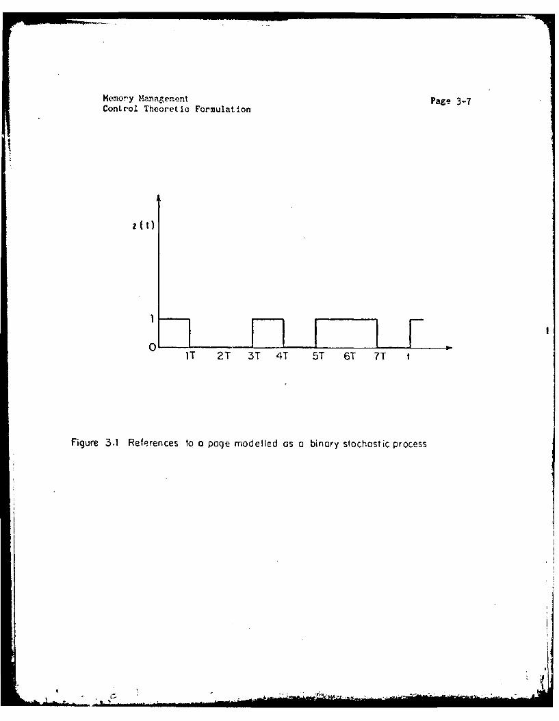
Me.mory Management Page 3-7Control Theoretic Formulation
z t)
II
Figure 3.1 References to a page modelled as a binary stochastic process

Memory Management Page 3-8Cost Expression
%3 COST EXPRESSION
In this section we derive an expression for the cost of imperfect
prediction. In memory management with fixed memory partitioning,
generally the objective is to minimize the chances of page faults. In
the ease of variable partitioning, however, page faults alone do not
provide an adequate criterion. Ihis is because it is always possible to
reduce page faults for one particular program by giving it more memory.
This, however, penalizes other programs which must operate with less
memory. Thus, an additional objective is to keep memory usage also to a
minimum. This second cost is often referred to as space time product.
The total cost is, therefore, calculated as follows.
Let H = Cost of a page fault
= Cost of bringing a new page in to memory
and U = Cost of memory usage
= Cost of withholding one page of memory from other
users for unit time
Let V(k) denote the predicted value of z(k) from information available
at time (k-1)T. Due to imperfect knowledge of the future, z(k) and i(k)
are not the same. A price has to be paid for errors in prediction. If
both z and i can take only 0, 1 values, then there are only 4 cases to
be considered as shown in Table 3.1.
Thus the additional cost due to imperfect prediction of z is given
by
C 2 Rzi + Ulii
4k-

Memory Management Page 3-9Cost Expression
TABLE ., : Costs of memory management
Decision Additionalz I Based on 1 Cost Remark
0 0 Remove 0
0 1 Keep UT The page is not referencedbut still kept.
1 0 Remove R A page fault occurs.
1 1 Keep 0 The page is referenced andit is in the memory.
Our aim should be choose i such that the expected cost E[C] is minimum.
E[C] = E[RzE + UTZ!]
If we choose our decision interval T such that T:R/U or R:UT, we have
E[C] E[ R(z! + 1)]
- E[ R(z-R) 2 ]
=R E[(z-i) 2 ]
- R times the mean square prediction error
Note that the second equality above holds only if both z and z are
zero-one valued variables, not otherwise.
A classic solution to the least square prediction problem is due
to Wiener(Pap65, p. 408]. lt consists of designing a linear system
(Wiener filter) with impulse response h(u) such that the output of the
system is the estimate i(t) when input is z(k), 0 < k < t-1 (see
Figure 3.2).
L.b(u)z(t-u)u21
The Impulse response h(u) can be obtained by solving the Wiener-Hopf

Memory Mhinagemi-'nt Page 3-10Cost Expressioii
Post Linear Systemn Peice
votions, hU)
Figjure 3.2: Wiener filter predictcor. h (u) is given bysolution to Wiener-Hopt equation,

Memory Management Page 3-11
Cost Expression
equation
C(k) t(k-u)h(u) k:O, 1, 2,
u=1
where C(k) = autocorrelation function of z(t). The memory management
problem can, therefore, be solved by measuring C(k) and solving the
Wiener-Hopf equation.
Strictly speaking the Wiener filter technique is not applicable to
binary processes. For example, the output of the predictor will not be
necessarily 0 or 1. It may take any Value. The analysis is, therefore,
approximate. The reason for the choice of this method for initial
analysis is that there is no as convenient a way of modeling binary
processes* as for continuous processes. In fact, the techniques for
modeling, estimation, and prediction of continuous processes are so well
developed that it is no longer necessary to solve the Wiener-Hopf
equation in order to find the optimal predictor. Simply, by looking at
the shape of the autocorrelation function, it is possible to guess the
model of the system that could have generated the process [BoJ70 &
Nel73J. For example, an exponentially decayinR autocorrelation function
implies an AR(1) model, i.e., the impulse response h(u) (the solution of
the Wiener-Hopf equation) is zero every where except at u=1. These
"Time Series Analysis Techniques" provide very convenient means for
modeling empirical data.
---------------------------------------------------* We have developed some techniques for modeling biniry processes.These techniques and their applications to page reference process aredescribed in the next chipter. In this chapter we report the resuttsusing conventional techniques.
- -

Memory Management Page 3-12Non-stat ionaiity
3.4NO-STATIONARITY OF THE PAGE REFEREjCE PROCESS
Arnold [Arn75] has reported the results of autocorrelation
measurements on a number of programs. His conclusion is that in most
cases the autocorrelation function has the following form
C(k) = p + (1-p)qk with p > 0 and q:constant
Arnold reports in his paper that one of the main findings of his
measurements is the fact that the autocorrelation function does not ao
to zero, i.e., the constant piO.
An important implication of this observation is that the page
reference process is a non-stationary stochastic process. In fact, a
commonly used test for stationarity is to verify that the
autocorrelation function C(k) dies down to zero ?t large lass (PoJ70].
A simple explanation is that if the correlation between z(k) and z(O) is
zero for large k, the effect of the initial conditions will not be felt
after large enough k, and the process will eventually reach a state of
"statistical equilibrium" called stationarity.
There are unlimited number of ways in which a process cn be
non-stationary. However, mest of the real world non-stationary
processes exhibit a "homogeneou" non-stationary behavior such that sonv
suitable difference of the process is stationary. For example, If tn'
process exhibits homogeneity in the sense that apart from local level
( i.e., local mean ), one part of' the series behgves much like any other
part, then the first differencc of the process may be found t( be
_ _ _ ... . . . . .... . ... . .. .. . . ... .... .. . . . . f

Memory Management Page 3-13
Non-statlonarity
stationary.
To model such non-stationary processes, therefore, one studies the
autocorrelation function of 1st, 2nd, 3rd, ... differences until a
stationary process is obtained. Thus, to model z(t) we should study the
autocorrelation functions of
Dz(t) z(t) - z(t-1)
D2z(t) Dz(t) - Dz(t-1)
Ddz(t) Dd-lz(t) - Dd-lz(t-l)
till a stationary process Ddz(t) is found.
The non-stationarity of page reference process z(t) can be
explained as follows. Even though the program behavior may be
stationary in one locality, the frequency of reference to a particular
page varies as the program progresses from one locality to the next.
Thus, the process z(t) may behave like a set of locally stationary
processes, i.e., like a homogeneous non-st3'.ionary process whose mean
value varies. If this is so, the first difference of z(t) must be
stationary. At this point this is just a hypothesis. The
identification results presented in the next section confirm this
hypot hesis.
Memory Management Page 3-14ARIMA Model
. ARIMA MODEL OF PAGE REFERENCE BEHAVIOR
This section describes the results of modeling the 1st and higher
differences of the page reference process. The data for analysis was
supplied by Arnold. It consisted of a reference string trace of the
MUDDLE compiler. About 5 different pages were chosen for analysis.
The autocorrelation functions of some of the pages studied is
shown in Figure 3.3. The broken lines indicate the 95% confidence
interval of the ACF for the given sample. It is obvious frcm this
figure that the process is non-stationary and further differencing is
necessary. The first difference process y(t) is defined as
y(t) = z2.)-z(t-1)
In almost all cases studied the first differences turned out to be
stationary. Sample autocorrelation (ACF) and partial autccorrelation
(PACF) functions are shown in Figure 3.4. The common characteristics of
these functions and the inferences that we can draw from these are now
described.
A. The ACF cuts off at large jags This implies that the 1st
differences are stationary and no further differencing is neccesary.
Thus the appropriate model for the page reference process z(t) would be
an ARIMA(p,I,q) model (Puto-Regressive Integrated Movin7 Average model
of order p,1,q) for some suitable p, and q.

AD-AUG 392 HARVARD UNIV CAMBRIDGE MA AIKEN COMPUTATION LAB F/6 9/2CONTROL-THEORETIC FORMULATION OF OPERATING SYSTEMS RESOURCE MAN--ETC(U)MAY 78 R K JAIN N0001-76-C-Og14
UNCLASSIFIED TR-10-78 NL
.3 /II/EEI/EI/EIIEEIIEIIIIEIIIIIIIIIIIIIIIffllfllfIEEEEEEEIIIIEEEIIIIIEEEEEIIEIIIIIIIIIIIIIIlfflffl

Iltli 8D2
103%92~
22111
--L-4
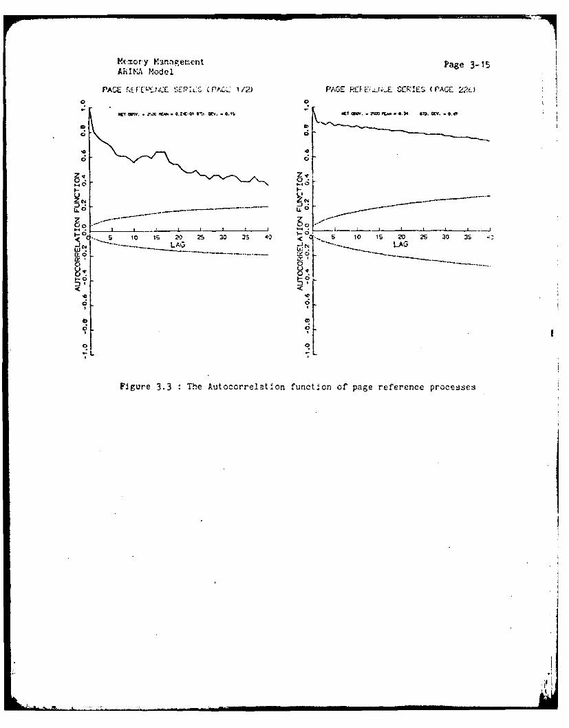
Vcicory MannermentPae31ARINA M-odelPae31
PACE SzE' ~ Er.ELl CPA 112) PACERfrE SERIE$. (PAGE 220D
o 0
0'
ILOz
5 10 is 20 25 0 33 420.. 5 10 is 20 25 20 4"
-.----. LAG - ,LAGw~ w
00
00
M-

Mtrmory Mingrment Page 3-16ARMMA Mcdel
1ST ('1FF. OF N-S RIT. 'PEE, UAL79 I ST rl';F. OF frnE RCF. SERIES '
17 QWV. *24P# MW C .4ZW UY r .MV[.I ~V 0.2 30M 0S." * . 'L a C. sl . .7
C;
Ib-I 0 ,.0 0
IfLAC,.J LAG
1-- 0
0'C!
OC IAI 2"CMW W. FW.Q.-c ) E. 02
r) 0
o <JC E-V .. . .4 .E .. ... ... ... . ..... .. .. .8 . . . ..................... I.C £~* 1V.
i. c. 01U'U: -!. II
0
-J6i
ZCV It0.L.
C! 0l
FI ur 3. h C n AFo s i-frnoo h: 'Cre,,enp

Memory Management Page 3-17ARIMA Model
B. The mean of the difference Drpobess 15jQ z.r This means that
the constant term in the ARMA model for y(t) could be taken as zero.
This property of y(t) is least surprising because a little arithmetic
shows that this must be so.
yMt = z(t)-z(t-1)
Hence, mean of y(t) = N1
t=:2
= [z(t)-z(t-1)]t=:2
z(N)-z(l)N-1
=0 or -L-N-1
C. Both ACF and PACF are laresL Al la afte which they die cut
slowly. Of course, there are a few jumps at other lags* and the fall is
not smooth. The main point is that C(I) and 0(l) are not insignificant
as was the case for CPU demand processes. Therefore, suitable low order
model for y(t) is ARMA(I,1) model. To see this clearly, consider the
* Some pages show periodic peaks in the ACF even at large lags. Thishappens for the pages that are in a big (with respect to interval T)program loop. If the total time of the loop is kT (say), the page isreferenced every k intervals. Thus z(t) and z(t+k) are highlycorrelated, and so are z(t) and z(t+jk), J=2,3,... This will causepeaks in ACF at lags jk, J=1,2,3,... In conventional time seriesanalysis this behavior is called "seasonal". Though it is not verydifficult to model this behavior, we will not consider this here inorder to keep the analysis simple.
---- -

Memory Management Page 3-18ARiMA Model
ARMA model
y(t) - ay(t-1) e(t) - be(t-1)
The ACF and PACF of this process for different relative values of
parameters a and b are shown in Figure 3.5. The exact expressions are
as follows
C(O) = 1 0(0) 1
C(1) = a-bC(1) 0(1) = a-b
1-2ab+b2
C(k+l) = aC(k) k>O 0(k+1) = bO(k) k>0
The comparison of Figure 3.4 with Figure 3.5 shows that a
ARMA(1,1) model with b>a>O could be used for y(t).
D. The ACF as well PACF are negaIve at la J., This observation along
with the expressions for C(I) and 0(1) given above further confirm the
constraint guessed above, i.e., b>a. Tne fact that the successive
values of y(t) will always be negatively correlated can easily be seen
as follows:
y(t)=1 => z(t):1 => y(t+l)=O or -1
y(t)=-1 => z(t)=O => y(t+1)=O or I
Thus a positive value of' y(t) implies that that the next value will be
zero or negative and vice versa.
The parameter vilues obtained fer the cases analyzed Pre listed in
Table 3.2. Notice that a and b do satisfy the constraints (b>i>O)
conjectured above. In addition we notice that b is almost always nearer
to 1 and a is nearer to 0. Also listed in the table is thf relative
.p.- ,, .

* Memory Management Page 3-19ARIMA Model
,b
1.0 _ _ _ _ _ _ _ _ _ _ _ _ _
Ck kkk
Ck ' kk
Ck Okk1.
-I.00
~~Okk
-1 .0
Figure 3.5: Autocorrelation and partial autocorrelation functions Ck and Okk
for ARMA (1,I) Modely(1) - ay(t-1) e (t -be(t-1)
- I -.

Memory Management Page 3-20ARIMA Model
TABLE _,2 Parameter values for the ARIMA(1,1,1) model
(1-aB)(1-B)z(t) = (1-bB)e(t)
-------------------------------------------------------------
Page # a b R2
44 0.654 0.961 14.1%
79 0.446 0.856 17.3%
172 0.345 0.822 20.6%
206 0.0 0.858 41.4%
226 0.0 0.783 38.2%
reduction in the variance (R2 ) achieved by the model. Notice that the
model does provide significant gain in prediction efficiency over a
zeroth order model.
The fact that ARMA(1,1) is the appropriate low order model for
y(t) is further confirmed by comparing it with other low order models
like AR(1), MA(1), or AR(2). The relative efficiency of these models is
listed in Table 3.3. Notice that in all cases analyzed, the ARMA(1,1)
model turns out to be the most efficient.
Since y(t) is the first difference process of z(t), z(t) is said
to be the first "integrated" process of y(t). Thus an Auto Regressive
Moving Average (ARMA) model of order 1,1 for y(t) implies an Auto
Regressive Integrated Moving Average (ARIMA) model of order 1,1,1 for
z(t). The model equation for y(t) is
'I

Memory Management Page 3-21ARIMA Model
(1-aB)y(t) (1-bB)e(t)
where B is the backward shift operator (By(t) = y(t-1)). Further since,
y(t) = z(t)-z(t-1) = (1-B)z(t)
the model equation for z(t) is given by the following equation
(1-aS)(1-B)z(t) = (1-bB)e(t)
TABLE . : Comparison of ARMA models of 1st difference process
y(t) = z(t) - z(t-1)
List of R2 (5 reduction in variance) for different models of y(t)
Page # AR(1) AR(2) MA(1) ARMA(1,1)
44 4.6% 6.0% 6.4% 14.1%
79 7.6% 13.2% 17.3%
172 13.2% 16.9% 19.1% 20.6%
206 25.0% 29.0% 41.4% 41.4%
226 25.4% 29.5% 38.2% 38.2%
-- -------- -------- -------- ------

Memory Management Page 3-22Page Reference Prediction
3.6 PAGE REFERENCE PREDICTION USING THP ARML1 1l M.D
The net conclusion of the last section is that the page reference
behavior of programs can be appropriately modeled by an ARIMA(1,1,1)
model
(1-aB)(1-E)z(t)=(1-bB)e(t)
where z(t) is the binary page reference process, e(t) is white noise, 2
is the backward shift operator, and a, b are model parameters with
b>a>O. Using this model, we can derive equations for prediction of z(t)
based on process observations up to time t-1. In the followinF, we
derive two such sets of equations called "open loop" and "closed loop"
predictors. An implementation of open loop predictor using two
exponential weighted averages is also discussed.
3.6.1 Oen Loop Prcdictor : The usual way to derivc a predictor for any
ARIMA model is to transform it into an equivalent AR model. For our
ARIMA(I,1,1) model, this is done as follows:
e(t) =----a--)- z(t)1-bB
I1- (l+a-b)B -(b-s)(1-b) 2 z(t)i=2
= z(t)-(l+a-b)z(t-)-(b-a)(1-b) i-2z(t-i).i:2
or, z(t) = e(t)+(1+a-h)z(t-1)+(b-a)(1-b) "F i2g tiL-i=2
*1
. . . . . ,. *o - -....- - ~ -. - - -

Memory Management Page 3-23Page Reference Prediction
Since e(t) is white noise and can not be estimated or predicted
from the previous observations, the best estimate of z(t) from
observations up to time t-1 is given by:
2(t)= (1+a-b)z(t-1)+(b-a)(1-b) lbl-2z~t-l )4-bi t± [3.1)i=2
This equation is very inconvenient to use because it requires knowledge
of all previous observations. One way to simplify it is to ignore the
higher order terms (terms with small coefficients). In practice, terms
after the 5th lag can be easily ignored without much loss in accuracy.
A more ingenious procedure is to rewrite the equation 3.1 as
follows:
i(t) = (1-c)z(t-1) + c z(t-2) [3.2]
where c=b-a>O and z(t-2) is defined as (1-b) times the summation term in
the equation 3.1. It can be recursively calculated as follows:
(t-2) = (1-b)z(t-2) + b2(t-3) with 2(0)=0 [3.3]
Notice that both the equations 3.2 and 3.3 represent exponential
weighted averages. However, the weighting coefficients in the two
equations are quite different, because b-c = a 1 0.
E .9._-. : A somewhat different equstion for the
predictor can be derived as follows:
z(t) I-bB(1-aB)(1-B) e(t)
"e(t) +-(-----------P,(0)
(1 a-b) - aB=e~t) +------------e~t(1-aH)( 1-2) et
0'.A

Memory Management Page 3-?24Page Reference Prediction
= et).-b- aP (1-aB)(1-B)= et) (1-aB)(1-B) -b Z(t-1)
=e(t) + (I±2-b) -aB zt11-bb z(t)
Hence i(t) (l1a-b) -aB zt1I -bB ztl
or (I-bB)i(t) = (l~a-b) - aB~z(t-1)
or =()b2tl (1+a-b)z(t-l) -az(t-2)
or 1(t) =(l+a)z(t-l) - az(t-2) -~~-)-~-)
= (l~a)z(t-1) - az(t-2) -be(t-l) (3.4)J
where e(t) =z(t)-z(t)
"Error in prediction at t
"Innovation sequence
The block diagram representations of predictors given by equpt ion 3
and 3.4~ are shown in Figure 3.6. It is obvious from the diagramns why w
call these predictors open loop and closed loop respectively.
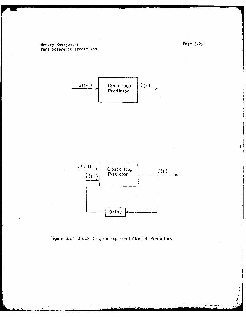
Mrmory Manngernent Page 3-25Page Reference Fredictiocn
z(t-1) Open loop 2(t>1Predictor
zI ____
Figure 3.6: Block Diagram representation of Predictors

Memory Management Page 3-26ARIMA Algorithm
3. ARIMA PAGE REPLACEMENT ALGORITHM
Using either the open loop exponential predictor or the closed
loop equation derived above, one can design a page replacement
algorithm. We will call such an algorithm "ARIMA page replacement
algorithm". In the following, we describe the algorithm based on the
exponential pradictor. The closed loop version can, similarly, be
designed. The algorithm is as follows.
1. Associated with each page i is a hardware register 7i (called
2-register). Also associated is a bit zi (called z-bit).
2. Whenever a page is referenced ite associated z-bit is set.
3. Every T interval (where T is the ratio of costs as described
before), all Z-registers are updated using the following (FORTRAN
like) statement :
21 = (1-b)*zi + b*zi
and all z-bits are cleared.
4. When a new page is loaded in the memory the zi bit is cleared ard
2 is initialized to 0.
5. At the time of pawe replacement, which could bc every T interval,
or more appropriately at page fault, a quantity called £i is
calculated as follows
i (1-)z + *i
Based on z a decision is made regaring the page to be rrplnced.

Memory Management Page 3-27ARIMA Algorithm
There are many possible ways of making this decision. Some
examples of such decision rules are described below
a. The page with least ii is replaced.
b. All pages with ii < k, where k is some suitable cut off point
(say 0.5) are replaced.
c. The first page encountered with ii < k is replaced.
d. Among the pages with z < k, the page to be replaced is
selected using LIFO, FIFO, or LRU algorithms.
Of course, one may also use a combination of two or more rules,
for example, in the case b above, if there is no page with ii < k, then
use the rule a, or try varying k depending upon the page fault frequency
and so on.
The main overhead involved in this algorithm is the update of Z
registers every T interval. This overhead is not excessive considering
that it involves only one multiplication, one addition, and a
complementation. A simple hardware circuitry could be used to do this
task as shown in Figure 3.7. At the time of replacement the same
circuitry could be used for prediction by replacing b by c.
The question that we have ignored so far is what value of
parameters b and c should be used in the ARIMA algorithm. Ideally, one
would like to estimate these parameters separately for each page. The
estimation technique should be an adaptive one so that bi and ci are
updated along with zI every T-interval. Alternately one could use some
suitable fixed value. This latter procedure has much less overhead and
I.!

Memorwy Manc:nt Pc3-28AfRIM Algor.t hm
c N0 D
b (or c)m -I-bz
D~ (or 4z)
7-regisler T.
Figure 3.7: Hardware Implemenlation of ARINIA Algorithm
A '

Memory Management Page 3-29ARIMA Algorithm
is more practical. However, in this case, program behavior monitoring
should be done from time to time to detect drastic variations in user
program behavior. The main consideration in choosing these values is
that they should be representative of user program behavior, and also
they must be easy to represent. For example, for the pages we analyzed,
we found that the average values of b and c were 0.856, and 0.567
respectively. Therefore, b=7/8, and c=1/2 seem appropriate, considering
that we are going to use binary arithmetic.

Memory Management Page 3-30Special Cases of ARIMA
_.8 SPECIAL CASES OF THE ARIMA ALGORI-_U
In this section we show that working set, roference frequency, and
few other algorithms are special cases of the ARIMA algorithm. tnother
special case is an extended working set, wherein the window size is
dynamically adjusted to match the pror-ram loca. ty size. Recall from
the last section that the exponential predictor Cor the ARIMA(I,1,1)
model is given by
i(t) = (1-c)z(t-1) + cz(t-2)
Z(t-2) = (1-b)z(t-2) + bz(t-3)
We shall refer to these two equations as prediction equation, and update
equation respectlveiy. ine iour special cases of the tRI.-A aiorithm
occur when the parameters b and c take their extreme values 0 and 1.
These cases are now described.
Case I i.--O : In this case, the prediction equation becomes
i(t) = z(t-1)
i.e., the pages that were referenced in the last T interval are the oncs
that are likely to be referenced in the next T interval. All other
pages can be replaced. This is exactly what YQtrjn &I policy also
says. For this special case of the ARIMA pane replacement algorithm
described above, the 2-registers are no longer necessary, and the pnces
with z-bit on constitute the working set. Also notice that c~b-qrO
implies that the model equation for this case is
(1-B)z(t) = e(t)
i.e., an ARIMA(0,1,0) model. In this case the process z(t) is an
,l

Memory Management Page 3-31Special Cases of ARIMA
"Integrated white noise" or Wiener process. Thus working set is optimal
for programs whose page reference processes constitute a Wiener process.
Since using WS is equivalent to using a white noise model for the
first difference process y(t), the percentage improvements listed in
Table 3.3 are also percentage paging cost improvements achievable by
various ARIMA models.
Case II Lt : For this case the update equation takes the following
form :
2(t-2) = 2(t-3) = I (say)
i.e., the mean is time invariant, the prediction equation therefore
reduces to an AR(1) predictor :
i(t) = (1-c)z(t-1)+ct
This is Arnold's Wiener Filter model [Arn75]. Notice that this is
applicable only if the mean is time invariant, i.e., if the z(t) process
is stationary.
Case Ill lzl b= : For this special case, like case II above, the
update equation implies a time invariant mean and the predictor equation
becomes
i(t)=
i.e., the pages are expected to be referenced with fixed frequency (mean
value) and the page with least z is the candidate for replacement. This
is the Refenrece F neD.c polDicy of pa.ge replacement. This model is
also known as Indennti R e (IRM). For this case the
model equation becomes

Memory Management Page 3-3?Special Cases of ARIMA
(1-B)z(t) = (1-B)e(t) since a=b-c=O
or, z(t) = e(t)+z
This is an ARIMA(O,O,O) or white noise model. Thus the reference
frequency model is appropriate only if the page references constitute
white noise*.
Case IV J : In this case, the predictor and the update equations
become similar.
i(t) = (1-b)z(t-1) + bz(t-2)
2(t-2) = (1-b)z(t-2) + bZ(t-3)
These equations can be rewritten as follows:
i(t) r z(t-1)
2(t-1) = (1-b)z{t-1) + b2(t-l)
This is an extension of the independent reference model. Here the
reference frequency is assumed to be time varying and is computed
adaptively using an exponential weighted average. This policy could,
therefore, be called "Adaptive Independent Reference Model" (AIRM).
This is optimal when a=c-b=O and the process model is PRIMA(0,1,1):
(I-B)z(t) = (1-bB)e(t)
i.e., z(t) is the integration of a first order (colored or correlated)
noise. It could, therefore, be called "Colored Wiener Process".
# This same conclusion was reached by Aho, Denning, nd Ullman (ADU711.They call it Ao policy and show that the policy is optiml wlen theprobability of' reference of' a parle depends neither on timr(staticnarity) tior on previous progrram behavior (no-nutocorrelation).
- - - - .---
1- , OMAN
Memory Management Page 3-33Special Cases of ARIMA
We conclude this section on special cases of the ARIMA(I,1,1)
model by depicting all the four cases discussed above on a single
diagram as shown in Figure 3.8. The ARIMA model operates in the
triangular region O<c<b<1. It is obvious from this diagram that the
ARIMA(1,1,1) is a general model and that Working set, Arnold's Wiener
Filter, Independent Reference Model, and Adaptive Independent Reference
Model are all its boundary cases.
kI

Me mory MWnagcment Pase 3-34Special Cazes of' ARIMLA
Independent ReferenceC ~Model1/A"R P1A (O,,O
1.0
o <
WJorking set/ARi!,A I .0)__________
0 1.0 b
Figure 3.8: Special cases of ARINAA (1,1,1) Algorithm
* 7

Memory Management Page 3-35Limitations of the Formulation
3.9 LIMIA-ON- OF THE FORMU LMICN
In the lat. section it was shown that the working set policy is a
special case of the ARIMA policy. Therefore, a question that naturally
arises is whether there is any relation between the ARIMA and another
popular page replacement algorithm LRU, and whether the LRU is also a
special case of Lhe ARIMA. The answer is probably "no". This is
because of the limitations of the zero-one stochastic formulation that
we started with. It uses only a subset of the available past
informatlon.
de.per insight into the information structure can be obtained by
considering the information used by various algorithms. VMIN - the
optimal variable space algorithm uses the complete page reference
string. WS requires knowledge of set of pages referenced in the last T
interval. It does not require the order in which the pages are
referenced or the number of times they are referenced. A general ARIMA
model would use all the sets of pages referenced in successive T
interval. Finally, LRU uses the set of last referenced m pages along
with their order of reference. The Venn diagram of information used by
these algorithms is shown in Figure 3.9. The broken line in this figure
separates the past from the future. There are two inferences to be
drawn from this figure
.1
4

Memory Mcnigement Paso 3-3*-6Limitations or the Formnulat ion
WIN
Figure 3.9: information used by various page replacementolgorithms.

Memory Management Page 3-37Limitations of the Formulation
1. The information used by the WS is a subset of that used by the
ARIMA. This explains why ARIMA policies can always be specialized to WS
set policies with proper window sizes.
2. There is much information, ( like the frequency of reference of a
page in an interval, the order of reference of various pages, and
cross-correlation between different page processes ), that is not used
in the zero-one stochastic process formulation used to derive the ARIMA
policy. If we could somehow develop a formulation which uses the
complete past information, then both the WS and the LRU will be special
cases of the generalized model. The conclusions drawn would then be
universal in scope.

Memory Management Page 3-3PConclusion
1.10 COqLUSICNc
The page reference behavior modeled ao a zero-one binary
stochastic process exhibits a non-stationary behavior. An ARIMA(1,1,1)
model was shown to be appropriate for the process. This model is then
used to design a memory managenent policy.
The main results achieved in this chapter can be stated as
follows:
1. We have shown that the cost of imperfect prcdictior is
proportional to the square of the difference between the
predicted and tic actual value.
2. Using empirical results, we have shown that the ARIMA(1,1,1)
model is an appropriate model for page reference processes.
3. We have designed a new page replacement algorithm called ARI'MA
page replacement algorithm. The algoritnm is shown easy to
implement.
4. We have shown that many conventional algorithms like korking
Set, Reference frequency, and Arnold's Wiener Filter algorithm
are merely boundary cases of the ARIMA ilgorithm. Also we have
described conditions udder which these boundary cases re
optimal. In particular we, thus, have a control theoretic
derivation of the WS policy.
ga, w &'i lL

Memory Management Page 3-39Conclusion
In the analysis presented in this chapter, approximaticns were
introduced due to Gaussian assumption. We, therefore, expect that the
development of identification methods for discrete binary processes will
lead to better understanding and management of program memory behavior.

CHAPTE I v
1- -E- MODELS FOR BINARY PROCESSES
APPLqICTON TO MEM:-ORY t,&NGEMENtZ

Boolean Models Page 4-2Introduction
4,J INTRODUCTION
In this chapter we present a new approach for analysis of binary
processes. A process z(t) is called binary if the variable z(.) can
tak only two values 0 and 1*. A classic example of a binary stochastic
process is the so called "Semi-random Telegraph Signal", which consists
of a sequence of independent identically distributed binary random
variables.
In computer science, binary process are a common occurrence. For
example, as was shown in the last chapter, the reference pattern of a
particular page constitutes a binary stochastic process which can be
used to design new memory management policies. Similarly, in database
management, record reference patterns constitute binary processes which
can be used to detect changes in reference patterns and to determine
optimum points for database reorganization. In ,-..er neLwerks,
packet arrivals at a node can be modpled by a zero-one process. Several
similar examples can be constructed in the areas of weather prediction,
signal detection, medical diagnosis, and info ation theory.
-----------------------------------------------------------------------
In fact, z(.) can take any two values say a and b. The analysis
presented here can still be used by transforming It to another process
b-a " Notice that the process y(t) is a zero-one process.
•b I

Boolean Models Page 4-3Introduction
In spite of the fact that binary processes are so common, it is
surprising that no direct technique for identification and prediction of
such processes has been described in the published literature. The two
known methods for analyzing such processes are both indirect [CoL66].
In the first method, one analyzes the intervals between successive
z(t)=l pulses. These interval can be assumed to be Gaussian, and the
analysis carried out as usual. Alternatively, one can count the number
of z(t)=1 pulses over suitable intervals of equal length and model the
resulting "count" process as a Gaussian process. It is obvious that
both these approaches for "modeling" of the process are not suitable for
the prediction of z(t) given its history upto time t.
In this chapter, we present a direct approach to rodeling,
estimation, and prediction of binary processes. The apprcach i;
analogous to that for Gauss n processes. Like the Wiener filter for a
Gaussian process (see Figure 4.1), we design a system (a oclean system)
whose output is the predicted value i(t) , and the input is the past
history of the process. Our model is mere reneral than the Wiener
filter in the following respects:
1. The measure of goodness of the prcictor is not limited to a fixed
criterion, e.g., least-squares in the case of Wiener filter. Our
methcd applies to any given critericn: linear or non-linear.
2. We do not impose the lincarity ccndition on the system. Our method
gives the optimal non-linear predictor for the process. Further, if
the optimil predictor is not unique, our method gives all the
predictors.
....

Boolean ModelsIntroduction Page 1-1
Post History Future
O .Linear System Z)
a. Wiener Predictor for Goussion Processes
Post History Future
Z O,) ,. ,-, Booeon System z.. .
b. Booleon Predictor for 8inary and k-ory Processes
Figure 4.1: Analogy between Wizner predictor and
Boolean Predictor

Boolean Models Page 4-5Introduction
3. Our model is not restricted to stationary processes alone; it Is
applicable to some non-stationary processes also.
An additional feature of our model is that it gives zero-one
estimates of a zero-one process. Since z(t) is binary it is not
meaningful to have fractional estimates of z(t). For example, it is
meaningless to say 1(t) = 0.73 (though it is meaningful to say that the
probability of z(t) = 1 is 0.73 ).
The only restriction in our model, which does not appear in the
Wiener filter, is that the process is assumed to be Markov of a given
order n. A process is called Markov if the probability distribution of
z(t) given all the past history of the process depends only on a ffnite
past. In particular, z(t) is Markov of order n if
P[z(t)jz(1),z(2),...,z(t-1)] = Pfz(t)lz(t-n),z(t-n+1),...,z(t-1)]
Here P[.] denotes the probability of an event.
In this chapter we develop a general probabilistic model relatin,
z(t) to its past values. Based on this model, an expression is derived
for the likelihood function, and hence, for the maximum likelihood
estimates (MLE) of the model parameters. We show how the model is used
for optimum prediction and derive a formula for the totnl cost due to
prediction errors. Then we extend all results to the more general case
of k-ary processes. In this case, the process takes intei.er values from
0 through k-1. Finally, we show how the model can be used for paie
replacement.
b.* .~.1 ~ - - *-

Boolean Models Page 4-6Introduction
In the analysis presented in this paper we make frequent use of
the properties of pseudo-Boolean functions. The essential elements of
the theory of such functions are, therefore, briefly reviewed in the
next section (adopted from [HaR68]). The material in the other sections
of this paper is original and, as far as is known to the author, has not
appeared anywhere in the published literature.

Boolean Models Pare 4-7Boolean Functions
4.2 BOOLEAN FUCTION3 - FUNQAENTALS
The definition of Boolean functions varies widely among authorj.
In an attempt to generalize the concepts, even the pioneers of this
theory, Rudeanu and Hammer, have changed the definition over tire (e.7.,
in (HaR68], end (ud741). In this thesis, we adopt the following
definiticn from [HaR68].
4.2.1 Definition : By a "Boolean function" f(xl,x 2,...,xn) of n
variables we mean a mappingf:{O,11n->,,O,1]
i.e., a zero-one valued function of zero-one valued variables.
An example of a Boolean function is f(x1,x2 ) = x1 + x2 - ?xIy 2 .
The usual way to express a 2oolean function is by u ing the Boolean
operations (e.g., conjunction, disjunction, and negation). For rxaalpc,
the above function is usually written as
f(X1x 2 ) = x1x2 v x1i2
where ":" is the disjunction (inclusive OH) operator, bar indicates
negation, and conjunction is denoted by juxtaposition. The
transformation between the two representations is a result of' the
following equivalences:
I-x vx G[0,1]
x1 v x2 X1 + x2 - xlx 2 x, eo,
J
t

Boolean Models Page 4-8
A notation which is commonly used in the literature on Boolean
f'unct ions is the following
X0ZIt 1= X
Where x0 is "x sup 2ero" (not x raised to the power zero). To avoid
confusion, we will use (xi to denote the ith power of a binary variable
x. Continuing with the notation, if X = x1,x 2, ....XnJ is a set of' n
binary variables and 1 '2 ... .in is the n digit binary representAtion of'
i, Oe. i _1~, then
i Sin
qi(X) = i=xilx212 .. xni
is called the ith fundamental product. For example, for n=3
q5 = xlx 2 x 3 1=XJ 2x3 and qo =X 1 X 2 x 3 =t1 R2R3
An important property of' fundpmental products is that Oqi(X)=l if
and only if X~i. Thus, the fundamental products are "mutually
exclusive", i.e.,
to i
kqi i~j
There are many ways of' representing a Boolean function. A few
example~s are given below:
I- xI- x2 + 2x~x2 (polynomial form)
1' XX (Disjunctive Form)
(x 1 V X2)(Rl v R2) (Conjunctive Form)
I~xJ~x2(Reed-Muller form)
1' + IR2 +OX 1R2 KI (Sum of' Products form)

Boolean Models Fage 4-r,Boolean Functions
In our analysis, we use the sum of products form. Using 3h~nnon's
decomposition theorem, any Boolean function can be expressed in this
form as follows:
M() 2n-1Z_ fiqi(X)i=O
where, fi = f(XIX=i), i.e., f(X) when x1j=i, x2:i2 , ... , Xnin.
The concept of Booleen functions can be generalized to other
functions - not necessarily zero-one valued. Such functions are called
"pseudo-Boolean functions".
4.2.2 Definition : Let R be the field of real numbers; by 3
pseudo-Boolean function f we mean a mapping
f:1O,1} n --> R
i.e., a real valued function of bin3ry variables.
An example of pseudo-Foolean functions is the followirg function
f(x1'x2 ) = 0.5(xl)3 + 3xl - 2(x7) 2
In fact, all functions (including Boolean functions) of binary variables
are pseudo-Boolean functions. Therefore, the adjective "pseudo-Boolc-n"
may be droppcd whenever it is clear from the context.
Again using Shannon's decompo.-ition theorem, ony function of
binary varlablos can be reduced to a "sum of products form":n_
f(X) =.jfiqi(X)i=O
For example,
f(X 1 'x 2 ) = - 0"5(xi) 3 + 3x 1x2 - 2(x2)2
For this function F : 1, f 1 -1, f2 0.;, ind f. : I., hence,f 2 i
1'

Boolean Models Page 41-10Boolean Functions
f(X 1,x2) = xRl2 + (-l)Rlx 2 +t O.5xli2 + 1.5xlx2
Similarly, x 2eX1 o O1R2 + 1i~x2 + Ox1i2 + exlx 2
Notice that when expressed in the sum of products form, every
function of binary variables becomes linear in each variable (i.e., each
variable appears only as its first power), although the function itself
is non-linear (due to the presence of product terms).
LUI

Boolean Models Page 4-11Model Development
4 DEVELOPMENT OF THE BOOLEAN M EL
Let Zji denote the set of i observations immediately preceding
z(), i.e., {z(j-i), z(J-i+1), ... , z(j-)}. Thus
Ztti = (z(1),z(2),...z(t-1)) denotes the complete past history of the
process. Let Pt = P[z(t)=1:z(1),z(2),...,z(t-1)] denote the probability
of z(t):1 given the past history of the process. The simplest binary
process is the so-called "Binary Wh i" (BWN) or Bernoulli
Process. It is defined as the sequence of independent identically
distributed binary random variables. The semi-random telegraph signal
described previously is a BWN. Also if we associate a time index to
successive Bernoulli trials, they will constitute . BWN. A P'BN crn also
be obtained by filtering and clipping a Gaussian white noise. A BWN
with parameter p will be denoted by BWN(p)
For a Markov process of order n, pt depends only on the past n
values Ztn:fz(t-n),z(t.n+1),...,z(t1)1. We can represent the most
general non-linear dependence of Pt on Ztn by saying that pt = hZtn),
where h is some non-linear function of Z such that O(< h (I. In the
sum of products form, we have
Pt = P~z(t)=11'tn - ( iiZn 4.11
i=O
where h = h(Ztn!Ztn=i)
= Value of h(Ztn) when z(t-n),... z(t-1) take vplt'es
oorrespondir.7 to the binary expansion of i.
and ql(Ztn) ith fundamental proJuct. of zt-n),...,z(t-1)
tn)
- ) ~ i .' ".. . . . . _ . .. . ... . , :u -:: a- t, .i3'_.+... .t ',::J - . .E e . . - - - -, "

Boolean Models Page 4-1 2
Model Development
The equation for z(t) corresponding to this equation is
z(t) 2t I(*tqiZn 4.2)
where, ei(t) -BWN(hi).
By taking expectations of' both sides of equation (4.2) , it can be
shown to be equivalent to equation (*4.1). Notice that Zt. denotes the
"state" of the process. The process can be in any one of 2n states
corresponding to Z tni i=O,1,... 2 n-1* The distribution of the futurevalue z(t) in state i is Bernoulli with parameter h.
For example, the Boolean model of a second order Markov process is
+ e 3(t )z(t-2)z(t-1)
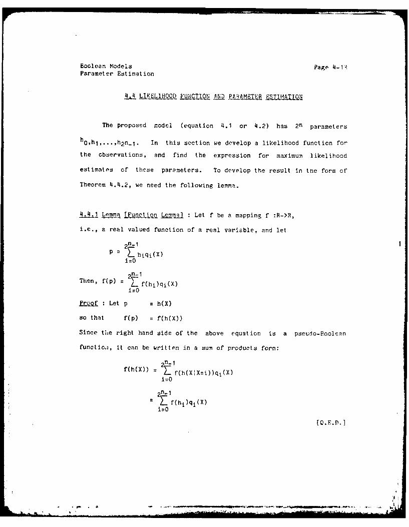
Boolean Models Page 4-IParameter Estimation
4.4 LIKELIHOOD FUNCTIONt !AD PAAMETER JQNTIAiTo.
The proposed model (equation 4.1 or 4.2) has 2n parameters
hohl,..,h2 n-1 . In this section we develop a likelihood function for
the observations, and find the expression for maximum likelihood
estimates of these parameters. To develop the result in the form of
Theorem 4.4.2, we need the following lemma.
4.4.1 Lemma [Function Lemmi] : Let f be a mapping f :R->R,
i.e., a real valued function of a real variable, and let
2 -1P -E hiqi(X)
i=O
Then, f(p) 2=Then f~p = Z_ f(hi)qi(X)
i=O
Proof : Let p = h(X)
so that f(p) = f(h(X))
Since the right hand side of the above equation is a pseudo-Boolean
functioa, it can be written in a sum of products form:
f~h(X =cf~h(X)) f(h(X:X~i))qi(X)
i:0
= fhi)qi(X)~i=O
[Q.E.P.]
__________________________________________________ b

Boolean Models Page 4-14Parameter Estimation
Some examples of the use of the Function Lemma are given below.
p2 = _ hi 2qi(X)i:O
= 1hi-qi(X)
i=O
1(1o ~g-p) = _ log(1-hi) qi(X)i=O
4.4.2 Theorem (Estimation Theoreml : The maximum likelihood estimate of
hi based on N observations {z(1), z(2), ..., z(N)1 is given by
mlh------------- 0 ,i..2 n -1
mio + mil
where miO = # of times the sequence Ztn=i is followed by z(t):O
and m i = # of times the sequence Ztn=i is followed by z(t)=:
Proof: Let H = {ho,hl, ... h2n_1 be the set of parameters.
Let, Pt P[z(t)=:1Zt,H] = hqi(Zt)
i=O
t - 1-Pt = PEz(t)=O!Ztn,H]
The above two equations for Pt and 5t can be combined as follows:
P[z(t)!Z tn,H] = P[z(t)=l:Ztn,H)z(t)Pcz(t):OlZtn,H) (t)
= p t ZMti(t)
Therefore,
Ptz(N),z(N-1),...,z(1):z(-n+l),z(-n+?),...,z(O),HI
= P[z(a)Iz(N-1),...,z(1),Z n,HIP[z(N_1)z(n_2),...,z(1),Z 1nH)...
.P[z( 1) nH ]
- *~*.
~i.

Bc .lean Mcdes Page 4.15Parameter Estimtion
T Plz(t):Ztn,H]
t=1
The above equation gives the likelihood that the N observations eare
from a model with parameter H = [ho,hl .h 2 n_,1 . Notice that we as6 l;me
the initial conditions z(-n+1),...,z(O) to be given (or to be assvT' ,
equal to zero). Only the parameters are to be estimated. The
likelihood function is
L(H) = 4 Zt)i(t)
ti=!1Pt (tp t)
taking the log- of the above equation ve cet the lol likelihood function
I(H) logL(H)}
Nr (z(t)1oE Pt + i(t) cy ptt=1
Now using the Function Lemma,
N N 2 -z(t)log Pt = ~t) (log h.)q (ztn )
t=l t=1 i:O
i:O t=1~ 2n-l_
In 11 mlog( hi)
i:O
where m
t:1
# of times Ztn~i is followed by z(t):l
The last equality Is a result of the obervaticn that z(t)qi(7tn )
if and only if z(t):1, and 7tn:i. Siniarly,
i ~.- .-. i--. ---

Boolean Modelt Page 4-16Parameter Estimation
t=1 =O
Therefore, the log likelihood function is given by
1(H Im1 iog h i + m 10 log(1-h i)1i=O
The maximum likelihood estimate of h.i is obtained by setting the first
derivative of the log likelihood function equal to zero, i.e.,
;h h. 1-h.
i mil
or h ------1 ~io + Mii
[Q.EMDli

Boolean Models Pae 4-17Measures of Goodness
4 MEASURES OF GOODNESS
In the case of Gaussian random variables it is common to define
the "best estimate" in the least-squares sense (LSE), i.e., 2 is the
best estimate of z if E[(z-2) 2] is minimum. In the case of binary
variables, the role is played by what we propose to call the "Least XOR
Estimate" (LXE), and the "Least Cost Estimate" (LCE).
3 Least XOR Estimate : Since both z and 2 can take only two values,
there are only 4 cases to be considered as shown below. Here e is used
to denote the error variable.
z 2 Error e
0 0 No 0
0 1 Yes 1
1 0 Yes 1
1 1 No 0
It is easy to see from the above table that e zoi (exclusive-or
of z and 2). The minimum number of error cases will be obtained if
E[zei) is minimum. The estimate i which minimizes E[ze.2 is the least
XOR estimate (also the least error estimate). it is easy to verify that
LXE is equivalent to LSE for binary variables, i.e., (7_i)2 = z% .
3.2 Least Cost Estimate : In formulating LXE, it wis assuned that both
kinds of error z=l,=O and z=O,2=1 are equally costly. In the sifnal
processing area, these two errors are called "ns' sicnl" and ",faIeC
S S

Boolean Models Page 4-18Measures of Goodness
alarm" respectively. The cost of these two types of errors is generally
different. For example, in the case of weather prediction, the cost of
predicting a storm and not actually getting one is quite different from
that of getting an unpredicted storm. Similarly, in the case of memory
management, the cost of a page fault (miss signal) is not always the
same as the cost of keeping an unused page for some time (false alarm).
In such cases, therefore, we propose a generalized concept to be
called the "least cost estimate" or LCE. In this case, the cost
function C(z,i) is a given, not necesarily linear, function of z anl £.
Now by Shannon's decomposition theorem, we can express C as follows
C(z,i) =Co + cI + C2 z + c3z
Where c0 = C(O,O), c = C(O,1), c2 = C(I,0), c3 = C(1,1).
Here c2 and e are the costs of a miss signal and a false alarm
respectively. Without loss of generality, we can assume that a0=c3=0"
This is because
C(z,i) = (c0 + c3z} + {(c1-co)iI + (c2-c3)zZ }
The part within the first set of braces is independent of 1, and hence
the problem is equivalent to one with cost of miss signal c2 _c3, cost of
false alarm elcO, and zero cost for correct prediction.
* | +

Boolean Models Page LI-19
Predict ion
4.6 LREDCLTO
We now return to our original problem of finding the Boolean
function g, such that the estimate i(t) = g(Ztn) minimizes a given cost
function. The prediction method that we are going to describe is based
on the two theorems below.
4.6.1 Theorem (Prediction Theorem : Given the model relating z(t) to
Ztn
2n1z(t) = r
= L- ei(t)qi(Ztn)i=O
the estimate i(t) which minimizes the expected value of cost funct ion
C(z(t),i(t)) for N observations is given by
(t) 2n -1E &iqi(Ztn)
iO
where ei, i=O,l,...,2 n -1 are zero-one valued variables chos n as
follows
/ 1, if hi > r
<< 0, if hi < r
d, if hi : r
cI
where r -------cl 1 C2
and d represents a "don't cire" condition, i.e., either 0 or 1 would do
equally well.
4'
-~ I

Boolean Models Page 4-20Prediction
Proof : Let the desired estimate be
(t) (Ztn )
where g(Ztn) is a Boolean function of Ztn. Again, using the
Decomposition Theorem, we have
2 n -1(%) T = / iqi(Ztn)
i=O
where e is a zero-one valued variable given by ei g(ZtnZtn=i)-
Since z(t) = ei(t)qi(Ztn)
i=0
the exclusion property of the fundamental products enables us to write
the cost function as follows:
C(z(t),i(t)) = Cl()( ) C z~t t
- 1 2( t +j c +c 2 ejt)7qj(2 n-1 2 n-1= I _ i(t) iqi(Ztn) + c2 /._et)q(t )
i=O i=O
=T1{e1 i~t)el+e2ei(t) i~qm( Ztn)
i=O
Taking expectation, we have2n-1
i :O
S C(hi, i)E[qi(Ztn)]
i=0
Thus we have decomposed the expected cost into 2n small components each
of which can be independently optimized. Consider the ith component
C(hi,6i):
C(hi,e I ) clhig i + c2hi i : c2 hi + i{c - (c + c2)hil
I + C2)hi

Boolean Models Page 4-21Prediction
The last expression is linear in e- it is minimum if each ei is chosen
as stated in the theorem.
[Q.E.D.]
Notice the similarity in expressions for z(t) and i(t). The
expression for (t) can be obtained from that for z(t) by replocing
ei(t) by el. In fact, ei is the best estimate of the binary white noise
ej(t) if the cost function is C(ei(t),6i).
4.6.2 Theorem [Total Cost Theoreml : The total cost of' imperfect
prediction for N observations by using the Prediction Theorem is
TC = 2 :
I min(c2mil, c-miO )
i=ON
Proof TCJ=1
(c12 (J) + e2z(i)l(j))j=1
NoNto 1 z L (J) L. iOqi(Zjr)iJ= z j = i=0
g ei r (j)qif'Zjn)
i:O j=1
i:O :
L= Cimi0
J=1 t=o
Hence, TC C _.e~mO+egml.i:O
II

Boolean Models Page 41-22Prediction
- min(cii, c2mil)i :0
The last equality follows from the observation that 91 is a binary
variable, hence the sum c1gimi + ci I either cjmj0 or c2mjj. The
prediction theorem chooses e. in such a way that the coefficient of the
larger term is zero.
[Q.E.D.]

Boolean Models Pave 4-23Tabular Method
4 TABULAR METHOD OF BINARY PRO E S PREDICTIO
This method is a result of combining the three theorems described
before, viz., the Estimation Theorem, the Prediction Theorem, and the
Total Cost Theorem. The method consists of the following steps t
1. Summarize the observed data in terms of frequency of occurrence of
various fundamental product terms. The summary is arranged in a
tabular form as shown in Table 4.1 . The table has 2n_1 rows and 5
columns. The columns are named Z, M, H, , and TC respectively.
2. The Z column consists of n subcolumns corresponding to n variables
z(t-n),z(t-n+1),...,z(t-1). The ith row in this column Is simply
3. The H column consists of 2 subcolumns corresponding to z(t)=O, and
z(t)=1 respectively. The entry in the ith row of the first
subcolumn is mio, i.e., the number of observations with z(t)=O ?nd
Ztn=i. Similarly, the entry in the second subcolumn is the number,
of observations with z(t)=l and Ztni"
4. The entries in the hi column are obtained from those in the M
column as follows
milmho + mil
entry In the z(t)=1 subeolumn
sum of entries In the z(t):1 and z(t):O subcolumns
5. The entries in the column are either 0, 1, or d according as h
is Icss than, vreater than, cr equal to the ratio r cl1(e I 4 e2 ).
"ip- -- ---- -. -~ - .~. I9

Boolean Models Page 4-24Tabular Method
If in a particular row, both miO, and mil are zero, the & entry in
that row is d.
6. The entries in the TC column are calculated according to the Total
Cost Theorem, i.e., the ith entry is min(c2mii clmi0)"
7. Synthesize the Boolean function represented by the column. This
is the optimum predictor. In sum of product form the function isn 1
simply t iqi(Ztn)"
i:08. The goodness of fit is given by the total cost calculated by
summing up the TC column.
We now illustrate the method with an example.
4.7.1 Example : The data consists of 144 observations on a 4th order
binary process. The actual observations have not been included here,
instead, the frequency of occurrence of the various combinations is
presented in Table 4.2. The cost of a false alarm is twice that of a2 2
miss signal, i.e., c1=2 and c2:1. The ratio r 2+i = i. The hi column
is constructed as usual. The entries in the column are I or 0
according as the entries in the hi column are greater or less than 2/3.
Two of the hi's are exactly equal to 2/3. Hence, the A entries in these
rows are "don't care" entries marked as d, and d2 respectively. The
predictor corresponding to d1d2 =O0 is
f(t ) =Z(t-)Z(t-3)Z(t-L)z(t-1) + z(t-4)z(t-3)z(t-?)z(t-1)
+ z(t-4)2(t-3)2(t-2)z(t-1) + z(t-4)z(t-3)z(t-2)Z(t-1)
+ z(t-4)z(t-3)z(t-2)z(t-1) + z(t-Z)z(t-3)z(t-2)z(t-1)
+ z(t-4)z(t-3)z(t-2)z(t-1)
* .*.~. *.*-1
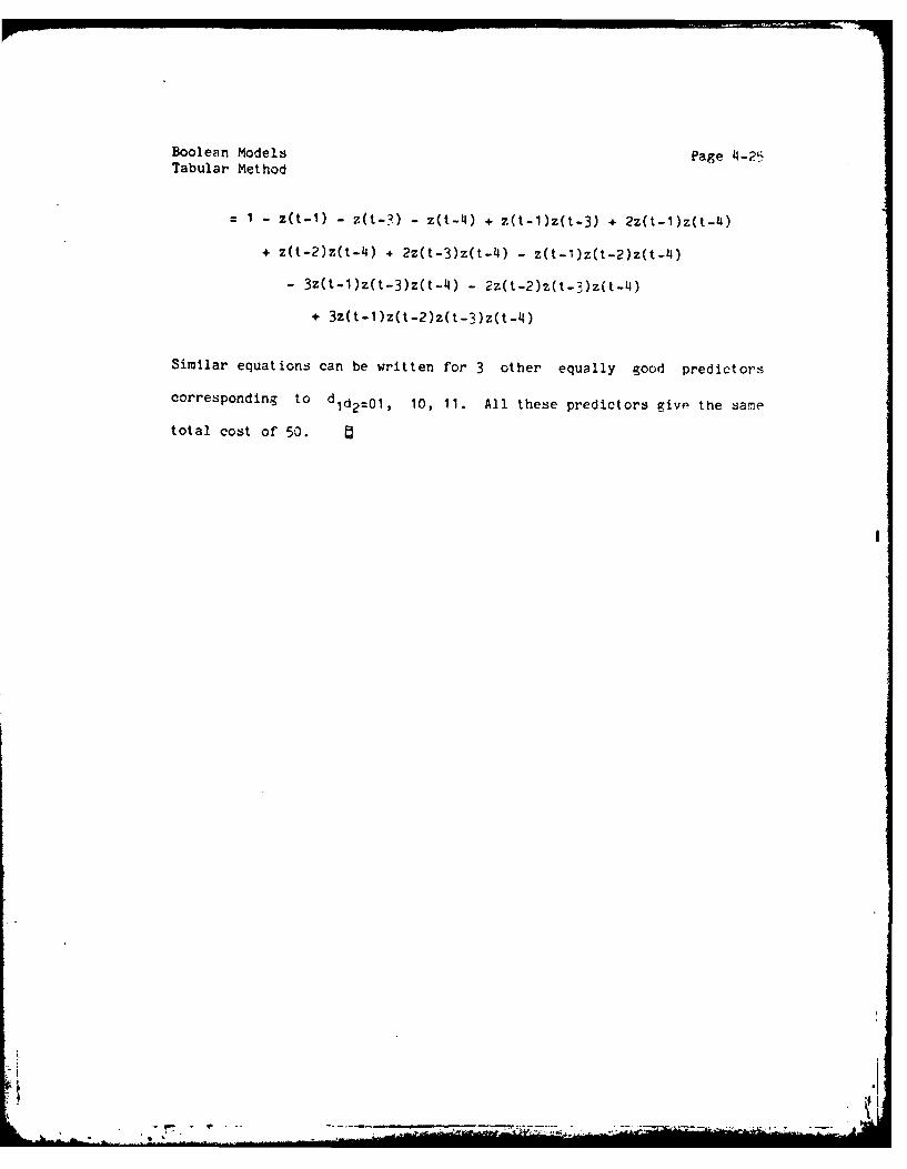
Boolean Models Page 4-25Tabular Method
1 - z(t-1) - z(t-?) - z(t-4) + z(t-1)z(t-3) + 2z(t-1)z(t-4)
+ z(t-2)z(t-4) + 2z(t-3)z(t-4) - z(t-1)z(t-2)z(t-4)
- 3z(t-1)z(t-3)z(t-4) - 2z(t-2)z(t-3)z(t-4)
+ 3z(t-1)z(t-2)z(t-3)z(t-4)
Similar equations can be written for 3 other equally good predictors
corresponding to dld 2 :01 ' 10, 11. All these predictors give the same
total cost of 50.
i

Boolean Models Page 4-26Tabular Method
TABLE 4.1 Tabular Arrangement for Boolean Model
# of obsv. with
o~-n ... 0~-2 0~-)Z t = ~ ~ l hig ~
o 0 1 M1 i .
o0 . 1 0 M 20 M21 ..
o0 * 1 1 1130 'p3 l
1 . 2n-l,O t2 2n_~,l

Boolean Models Psge 4-27Tabular Met hod
TAFLE 4.2 Fr~'quency Distribution for Data of' Example 4.7.1
0 0 0 0 1 9 0.90 1 2
0 0 0 1 8 2 0.20 0 2
o 0 1 0 3 8 0.73 1 6
0 0 1 1 7 1 0.13 01
0 1 0 0 3 2 0.110 0 2
0 1 0 1 9 7 0.144 0 7
0 1 1 0 2 14 0.67 d 4
0 1 1 1 6 0 0.00 0 0
1 0 0 0 5 3 0.38 0 3
1 0 0 1 1 2. C.89 1
1 0 1 0 2 9 0.82 1 14
1 0 1 1 0 7 1.00 1 0
1 1 0 0 2 8 0.80 1 14
1 1 0 1 7 5 0.42 0
1 1 1 0 1 2 0.67 d 2 2
1 1 1 1 3 9 0.75 1 6
Total Cost 50
- .f. U -------------- *-.-----Mika-----

Boolean Models Page 4-28Generalization to k-ary Variables
4.8 GENEHALIZATIQN TO K-ARY VARIABLES
In this section we generalize the analysis done so far to the case
where the process may take k values 0,1,...,k-1. To do this
generalization, we use the concept of Boolean functions extended for
k-ary variables. This concept is due to Rosenberg (HaR68, p. 301].
Let Bk = {0,I,...,k-1j. A Boolean function is now defined as a
mapping f : (Bk) n->Bk and a pseudo-Bcolean function as f : (Bk )n->R.
For any xGBcbc- , we define the so called "Lagrangean Development" xi (x sup
i) as :
kxl=x(x-l) ... (x-i+1)(x-i-1) ... (x-k+l)
mapping Bk into B2 . For example, when k=3:
x =(x-1)(x-2) x -x(x-2) 2 x(x-1)
Notice that
(1 if x=i
\0 otherwise
Let i,i2,...,in be the k-ary expansion of i, and X =xi,x2 ,...xn)
then Xi = qi(X) = x1 il x2i2 ... xnin
= ith Fundamental product
Any pseudo-Boolean function has a Lagrangean development (sum of
products form) :
f(xl,...,Xn) = .f(i)X L.._ fiqt(X)i=o i=O
NOW"4

Boolean Models Page 4-29Generalization to k-ary Variables
Again,
/ 1 if X=iqi(x) = <',
k 0 otherwise
Therefore, the fundamental products are mutually disjoint, i.e.,
/0 iijqi(x)qj(X) = ,
kqi(X) i:j
So, the Function Lemma holds, i.e., if f is a real valued function of a
real variable, and
if p =L_ hiqi (X)i:O
then f(p) = f(hi)qi(X)i=O
4.8.1 Fodel : The relationship between z(t) and Ztn in its most general
form is given by
z(t) = k .:lL. ei(t)qi(Ztn)i:O
where el(t) is a k. -ay whitLQ- I;i (sequence of independent identically
distributed random variables) with P[ei(t):u]=hiu. Hence,
Put = P[z(t)=uIZtn] = hiuqi (Ztn), u=0,1,...,k-1i=0
There is an additional constraint, however, that
u Put I
.is constraint ip' ries that
' I

Boolean Models Page 4-30Generalization to k-ary Variables
t hju : = , , . , n- 1
U=O
With this model, all the results of the binary case, viz.,
Estimation theorem, Measures of goodness, Prediction theorem, and Total
Cost theorem, can be generalized to the k-ary case. These
generalizations are stated below. The proofs of the theorems, being
similar to the binary case, are given in Appendix C.
4.8.2 Estimation Theorem : The maximum likelihood estimates of h.
based on N observations (z(1),z(2),...,z(N)} are given by
miu
TZ m iuu=O
where m.u = # of times Ztn-i is followed by z(t)=u.
.8. Measures of Goodness : In the case of k-ary variables the least
cost estimate 1(t) is obtained by minimizing a general cost function
C(z,£). The function can be expressed in the sum of products form as
follows :
C(z,f) = t uV u~v/uv z
u=O v=O
where Cuv = c(u,v) = cost of misprediction when z=u and i=v. It is
often easier to specify C as a k by k matrix whose (u+I,v+I)th element
is Cuv. A special case of the least cost estimate occurs when
C(z,2) I t.- zji£J2 J=0
L _

Boolean Models Page 4-31Generalization to k-ary Variables
It is easy to verify that in this case,
(0 if u:v
uv = <:kI otherwise
i.e., all errors cost the same. Thus, by minimizing this cost function,
one obtains the least number of errors. The estimate obtained could be
called "Least XOR Estimate", because of the form of the cost function.
In general, LXE is not the same as LSE except in the binary case.
4.8.4 Prediction Theorem: Given the model equation
z(t) = T el(t)qi(Ztn)
i=O
The estimate (t) which minimizes the expected value of the cost
function C(z(t),i(t)) is given by
-T_) = iqi(Ztn )
i=O
where , n - 1 are k-ary variables chosen as follows
e arg mnt cuvhiuu=O
arg minTv -- Cuvmiuu=O
4.8.4.1 Corollary : The least XOR estimate (cuv=l, uiv) is given by
arF max miv
4.8.5 Total Cost Theorem : Given a set of N observations on z(t), the
total cost of imper.fect prediction by usir.. the Prediction Theor,m is
TC .Z Wt miu:!uv
i=O u=O
1k------- - .
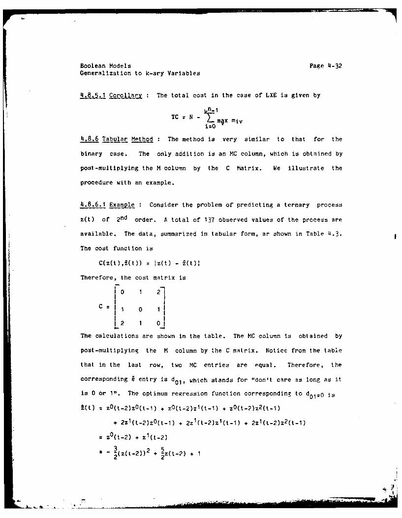
Boolean Models Page 4-32
Generalization to k-ary Variables
4.8.5.1 Corollary : The total cost in the case of LXE is given by
TC = N - T mQx miv
i=o
4.8.6 Tabul.ar Method : The method is very similar to that for the
binary case. The only addition is an MC column, which is obtained by
post-multiplying the M column by the C Matrix. We illustrate the
procedure with an example.
4.8.6.1 Example : Consider the problem of predicting a ternary process
z(t) of 2nd order. A total of 137 observed values of the process are
available. The data, summarized in tabular form, ar shown in Table L.3.
The cost function is
C(z(t),(t)) = Iz(t) i(t)I
Therefore, the cost matrix is
0 1 21I II I
C= 1 0 1I I
2 1 0
The calculations are shown in the table. The MC column is obtained by
post-multiplying the M column by the C matrix. Notice from the table
that in the last row, two MC entries are equal. Therefore, the
corresponding a entry is do1, which stands for "don't care as long as it
is 0 or 1". The optimum regression function corresponding to d0 1=0 is
i(t) : zO(t-2)zO(t-1) + zO(t-2)z1 (t-1) + zO(t-?)z 2 (t-1)
+ 2z1(t-2)zO(t-1) + 2z'(t-2)z1(t-1) + 2z1(t-2)z2 (t-1)
zO(t-2) + z1(t-2)
- (z(t-2)) 2 + z(t-2) + 1
24 2!

Boolean Models Page 1-43
Generalization to k-ary Variables
An equivalent, rather simple, expression fcr the above 2(t) is
i(t) = 1 +3 z(t-2) where +3 denotes "addition modulo 3".
A second predictor, corresponding to d0 1=1, can, similarly, be
written. The total cost in either case is 101.
Ak-

Boolean Models Page 4-34
Generalization to k-ary Variables
TABLE 4.3 : Boolean Predictor for Data of Example 4.8.6.1
z(t-2) z(t-1) mio miI m12 hio hi1 h12 MCo MC1 MC2 6i TCi
0 0 8 3 6 0.47 0.18 0.35 15 14 19 1 14
0 1 5 6 7 0.28 0.33 0.39 20 12 16 1 12
0 2 2 5 6 0.15 0.38 0.46 17 8 9 1 8
1 0 5 1 7 0.38 0.08 0.54 15 12 11 2 11
1 1 9 1 11 0.43 0.05 0.52 23 20 19 2 19
1 2 3 4 8 0.20 0.27 0.53 20 11 10 2 10
2 0 7 2 2 0.64 0.18 0.18 6 9 16 0 6
2 1 9 4 5 0.50 0.22 0.28 14 14 22 do1 "4
2 2 6 3 2 0.55 0.27 0.18 7 8 15 0 7
101
II

Boolean Models Page 4-35Model Order Determination
4.9 ON MODEL ORDER DETERMINTION
In "ie theory that we have developed so far we have assumed that
the model order n is known. In practice, this may not always be troe.
In the case of Gaussian processes there are many criteria and tests
(e.g., see [Aka74]), that allow us to determine an optimal model order
from empirical data. The corresponding results fcr Boolean models are
yet to be developed. Some rudimentary ideas on this problem are
presented in this section.
It should be obvious that the prediction error (or the total cost
of predicticn) monotonically decreases as the model ordcr is increased.
A quantitative formruo, for the increase in error is given by the
following theorem.
4.9.1 Theorem : The increase in cost in going from a (n+1)st order
model to nth order model is given by:
2n-1TC(n)-TC(n+I) [ min[ c2 (mil+mil), c1(mio+mi',)1
i=O- min(c 2mil, clmiO) - min(c 2mi,1, clmir,) ]
where the m-values are for the (n+1)st order model, and i'=2n+i.
Proof : Let m' denote the m-values for thp nth order model. For
example,
m1 0 of times Ztn = i is followed by z(t)=1
# of times z(t-n-1)=O, Ztni is followed by z(t)=1
+ 0 of times z(t-n-1):1, Ztn=i is followcd by z(t):1
, . - -. ..L:

Boolean Models Page 4-36Model Order Determination
of times Ztn+1 = i is followed by z(t)z1
+ # of times Ztn 1 = 2ni is followed by z(t)=1
=mil + mill
Similarly, m'lo = mio+mi,o
,n-lNow TC(n) = -min(c2m'il, cm'iO)
i=O
and TC(n ) _min(c2mil, clmj0 )i=O
= CZ [min(c 2mil, clmio) + min(c 2mill, clmiio))i=O
Notice that in the last equation the upper limit of the summation is
2n-I instead of 2 n+l-1. The difference of the above two equations gives
the theorem as stated.
[Q.E.D.)
There are two implications of this theorem. Firstly, each
summation term is of the form "the minimum of sums minus the sum of
minima". Hence, each term is non-negative. This proves the statement
that the cost monotonically goes down. The second implication, which
becomes obvious from the proof, is that the m-values for the nth order
model can be obtained from those of the (n+l)st order model by summing
up values that are 2n apart. Thus, once the data has been summarized in
a tabular form for high enough n, all lower order models can be easily
calculated. An example is shown in Table 4.4. Here m2 1 for the 2nd
order model is obtained by adding m21 and m6 1 (6 = 2+2n, n=2) of the rd
order model and so on. Thus, starting from a large n, one can calculate
V.

Boolean Models Page 4-37Model Order Determin3tion
the total cost TC(n) for that and all lower order models. A plot of
TC(n) vs n will look similar to that shown in Figure 4.2a.
In choosing the model order, a conpromise must be made between the
amount of computation required for the model and the improvement
obtainable by the model. The complexity of the model is exponential,
i.e., o(2n). Hence, the net utility of an nth order model is TC(n)-V2n,
where a is some normalizing constant. The optimal order is obviously
the one that maximizes this utility (see Figure 4.2). Another fact that
should be pointed out in this regard is that as the model order
increases, the number of parameters to be estimated increases and,
hence, the precision (or confidence) cf parameter values may go down.
As at present, we do not have formulae for parameter confidence.

Boolein Y'odels Page 4-38
Model Order Detertninat ton
Cost Computational Net(Error) Complexity Utility
I Optimal order
n n n
Figure 4.2:- Determination of model order n.
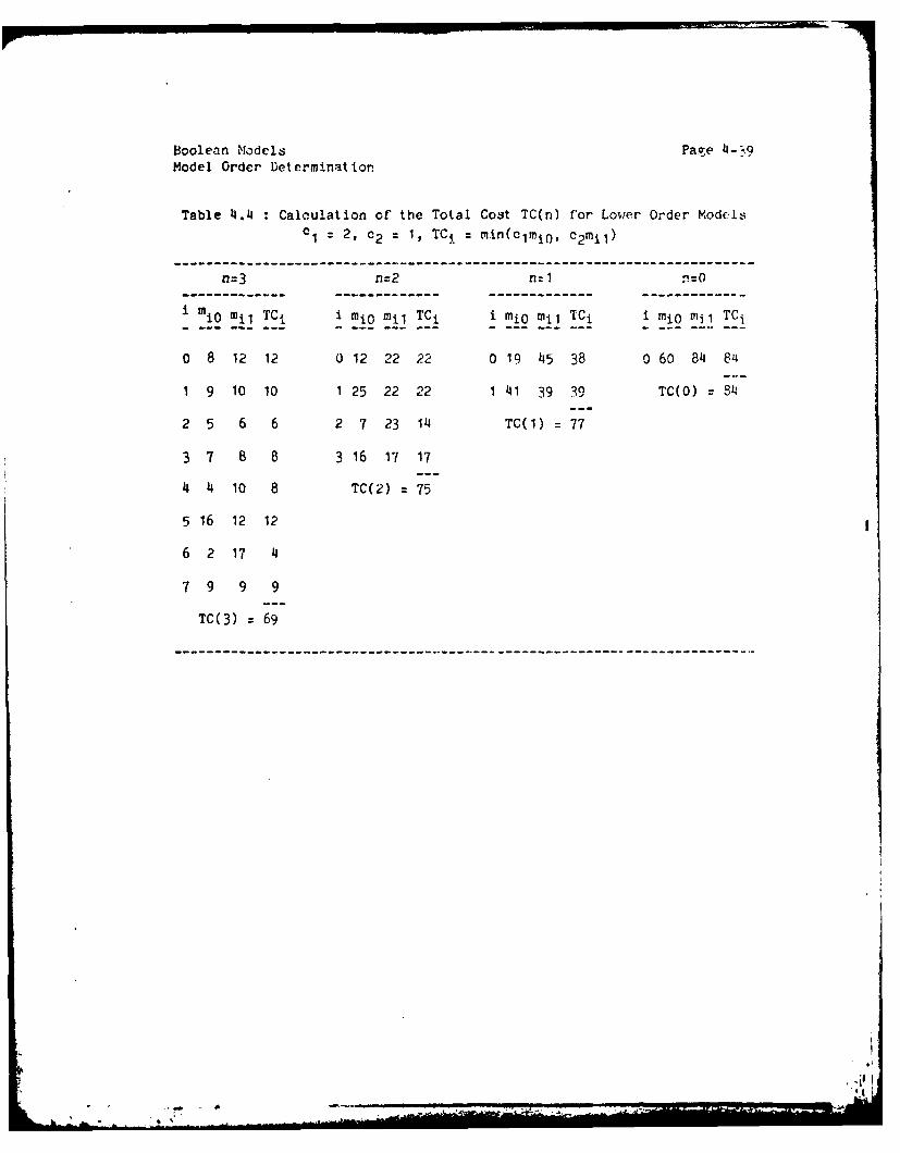
Boolean Models Page 4--9Model Order Determinatior.
Table 4.4 : Calculation of the Total Cost TC(n) for Lower Order Modcls01 = 2, 02 1 1, TCi = m.n(clmi(, c2mil)
n=3 n=2 n:1 n:0
i mio mi, TC, i mio mil TCi i mio il TCi i mio mjl TCi
0 8 12 12 0 12 22 22 0 19 45 38 0 60 84 84
1 9 10 10 1 25 22 22 1 41 39 39 TC(0) =4
2 5 6 6 2 7 23 14 TC(1) 77
3 7 8 8 3 16 17 17
4 4 10 8 TC(2) = 75
5 16 12 12
6 2 17 4
7 9 9 9
TC(3) = 69
-- - - - - - - -- - - - - - - -,-- --- - -- - - - - - - -- - - - - - - -

Boolean Models Page 4-40Stationarity
A stochastic process is called stationary if its probabilistic
behavior is independent of the time origin. In our Boolean model we
assumed P[z(t),Ztn] = h(Ztn) to be independent of time. For a
stationary process this is obviously a valid assumption. For a general
non-stationary process the model should be
Pztltn ] = hk't,Ztn) = L..hi(t)qi(Ztn)i=0
i.e., the model parameters are functions of time. We do not know how to
estimate these time varying parameters. Nor do we have any tests for
stationarity (similar to the ACF going to zero for continuous
processes). However, what we do know is that the time-independent
Boolean model applies also to the so called "Homogeneous non-stationary"
processes. A non-stationary process is called homogeneous if its dth
difference is stationary for some d. Recall that in the case of
continuous processes ARIMA rather than ARMA models are used to model
such homogeneous processes. The following theorem proves the above
statement.
Theorem : If the dth difference of a k-ary process z(t) follows an nth
order time-independent Boolean equation then the process Itself follows
a (d+n)th order time-independent equation.
Proof : Consider the Ist difference process y(t)
y() z(t) - z(t-1)So that t y(J) z(t)-z(O)
J21

Boolean Models Page U-41Stattonarity
Hence, P~z(t):Z tn.l ] P~z(t)lz(t-n-1), z(t-n),...,z(t-)]P z O +t Nn -. t 2
- ~ P (O ±ycjn:Z(O)+V 4-yjz(O)+) Jy(j)j=1 j=1 j=1
J=1
" prv(tH 7Z(rlt fL= P~~t~l(O)+ y(j}, y(t-n), y(t-n+l), ..., y~t-!)j
J=1
" Pfy(t):y(t-n), y(t-n+l), ..., y(t-1)]
" Independent of time if y(t) is nth order
Thus we see that if the first difference y(t) has r~th order
time-independent Boolean model, then z(t) has (n+l1)st order
time-independent model. By taking successive difference, the theorem
for dth difference follows.
[Q.E.D.]
The implication of this theorem is that we can use the thecry
developed so far for our page refergnce process whose Ist difference was
shown to be stationary in the last chapter.
4a--

Boolean L-.dels Page 4-42Page Replacement
4.11 PAGE REPLACEMENT USING THE BOLgAN MODL
There are two ways of using the Boolean model for page
replacement. The first is simply to use the model to predict z(t) from
the knowledge of z(t-1), ..., z(t-n). In this case, one must choose as
the modeling interval T = R/U, the ratio of replacement and usage costs.
As was shown in the last chapter, the cost criterion in this case 4s
least-squares. This method is straightforward and we do not develop it
any further here.
An alternative method arises from the fact that with the Boolean
model we are not restricted to the least-squares cost criterion. Hence,
we can design a page replacement policy without nny restriction on T.
In this section we develop such a policy. The policy is a realizable
version of a theoretically optimal, but unrealizable, policy called VMIN
[PrF76]. In order to see the optimality of VMIN, consider a particular
page. Without loss of generality, we can assume that the modelin7
interval T is unity. Supposing we know the complete page reference
process (past as well as future), let s be the length of time for which
the page is not referenced following t, i.e., z(t), z(t+1),..., z(t+s-1)
are all zero and z(t+s) is 1.
Let d(t) Decision to remove the page at time t.
( 1 ) page is removed= <i
0 => page is kept in the main memory
The cost of the decision d(t) over the interval (t, t+s) is
C = Rd(t) + sUd(t) = sU + (R-sU)d(t)
I,

Boolean Models Page 4-Lj3Page Replacement
Since the cost is linear in d(t), the optimal decision is d(t):1 iff
R-sU < 0, i.e., d(t)=1 iff s > -
U.
Thus the optimal policy is to keep the page if it is going to be
referenced in the next R/U interval. This is the VMIN policy. However,
this is unrealizable because it uses both past and future information.
A realizable version that uses only past information can be derived as
follows.
Since the future is unknown, the "forward recurrence time" s is a
random variable and the expected cost E[C] = Rd(t) + Ud(t)E~s is to be
minimized. The optimal decision based on the past information is,
therefore, to choose d(t)=1 iff E[s] is greater thin R/U. The
distribution of s, and hence its expected value can be derived from the
Boolean model of the process as described by the following two theorems.
4.11.1 Theorem* : The "reverse cumulative distribution" (1-tumulativc
distribution) of s is given by
riu Pfs>ulZtn=i]
- '=' h2Ji
• In this chapter we use the convention that whonever 4 appcars in a
subscript, the expression upto i is evaluated modulo 2n . Pnythir
following i is vimply another subscript. Thus riu is "i sub i comma u"I
whereas, h3 i is "h sub (3 times i modulo 2 n)",. For examp]", for n=2,
i=3, h3i:h9 =hl "

Boolean Models Page 4-44
Page Replacement
Proof _.. P s>O:Ztnil
= P[z(t)=OlZtnil
hi
r iu = Pls>u!Ztn=i]
" P[z(t+u):O, z(t+u-1)O, ... , z(t)=O:Ztn~i]
" P[z(t+u)=OIZtn=i,z(t)=O,...,z(tu1)zO]
P[z(t-u-1)=O,...,z(t)=OIZ tn=i]
" P[z(t+u)=Olzu+t,n=2i]r,uI
=h ri ,u-12 Ui
The above equation gives a recursive expression for riu" By applying
the recursion for successively decreasing value of u, and using the
initial condition rio we get the theorem as stated.
(Q.E.D.]
4~.11.1.1 Corollary :p iu =PIS=u!Ztn~i) h ui ::
Proof: Piu *riul - riu h WE h~
4.11.2 Theorem Let si = E(s!Ztn=i). Then, si is given by the
following recursive equation:
Si = hi(1+s2i) i=0,I,...,2 n - 1
00
and S 0 :

Boolean Models PEge 4-45Page Replacement
Proof s i Els5Ztn:i)
- u uPiuu=O
u(ri,u-1 - riu)u=O
(ro-ril) + 2(ril-ri2 ) + 3(ri2-ri3 ) +
rio + rjl + ri2 +
?I i + ri52i + 5i02i041 + ...
hi (1 + 2i + f2if4i + )
= !. (1 + s)2i
By substituting i=O, in the above equation we get
s 0 %0 (1+sO)
hoor s
Alternatively, one can derive an expression for s fro r
LuP[s=u:Ztn=O]. The result is the same as above.u:O [Q.E.D.]
Using theorem 4.11.2 one can get an expression for all sit
i=0,1,2,...,2n-I in terms of hi. However, one must follow a particular
order. After calculating si for i=v, calculate si for i=v/2 and
2n-1 +v/2. For example, for n=2 the following expressions are obtained.
ho mooSO = -- - ---
h0 m0 1
12 m20 m oo+in0 182 -------) -------) = -2 f 2( + s4 5 ( 1 + ' h 0 = m 2 0 + m 2 1 m 0 1

Boolean Models Page 4-46Page Replacement
h2 mlO m20(moo+m0l )
1 = R1(1+s2) = 1 (1 --- ( ------------)h0 10+M l m 1(m20+m2 1)
h2 m30 m2 0(m00 +m01 )3 = 3(1+s 6 ) = 3(1+s2) +3--- -) ( --- -)h0 m30+m31 1+o(m 20+m2 1)
Thus, using the<estimated value of the forward recurrence time for
the current state, one can decide whether to replace a page or not.
This version of the "VMIN" algorithm, although realizable, is too
expensive to implement in practice. This is because for an nth order
model 2n+1 registers are required to hold m-values. This number is
prohibitively large. Even for n=2, eight registers are required for
each page. To manage a page of 1048 words, using eight registers is not
economical. Therefore, at the present time we do not discuss
implementation aspects of the algorithms developed in this chapter.
However, with rapidly advancing memory technology it is quite possible
that pages of future will be much bigger and eight registers per page
would then not be an expensive proposition. If that happens, it might
be interesting to do empirical analysis of page reference process 3nd
develop a Boolean model of it.
~~,I

Boolean Models Page )4-47Conclusion
.6Z CqOLUSION
In this chapie" we have proposed a direct approach to modelin,
estimation, and prediction of a k-ary process. The process is modeled
as the output of a Boolean system driven by a set of k-ary white noises.
The model makes use of the special properties of pseudo-Boolan
functions in sum of products form. An expression for the likelihood
function has been developed. Using this expression a formula for
calculating the maximum likelihood estimate of the model parameters has
been derived. A method of finding the optimal non-linear predictor h:s
been developed. The method makes use of the :ample frequency
distributions of' the fundamental products.
Two different ways of' designing a memory management policies bsscd
on the Boolean model have been presented. The algorithms, althnu-h
physicaly realizable, are not economical enough for practical
implementation at the current state of technology. However, the
research reported here is valuable from the control-theoretic point of
view for applic3tion to other systems.
In the case of Gaussian variables, the Joint probability
distribution of n variables is completely specified by specifyin, thr
mean and covnriance matrix. Therefore, while analyzing Gaussinn
processes, we summarize the data in terms of the autccorrelnticn
function. In the case of binary varinbles, we find that autoeorrelitic-n
has no importance. Instead, tho rolc is played by nth orcir ,rcmr-nt, -

Boolean Models Page 4-48Conclusion
the expected values of fundamental product terms. Thus, whereas the
sufficient statistic' of a sample of n Gaussian variables has n(n + 1)/2
terms (n means, n(n-1)/2 variances), that of n binary variables has 2n-1
(kn-1 in the k-ary case) terms.
We have partly resolved the question of "representation". In the
case of Gaussian processes, the representation theorem [Ast7O] states
that every stationary stochastic process with rational spectral density
can be represented as the output of a linear system driven by white
noise. In this chapter, we have shown that any stationary finite order
Markov process can be represented as the output of a Boolean system
driven by a set of k-ary noises.
The Boolean approach to the analysis of k-ary process parallels to
that conventionally used for Gaussian processes. However, as this is
the first time that this approach has been taken, many issues remain to
be resolved. In particular, the problem of order determination needs
further research. Nevertheless, some of the results obtained are more
general than those known for Gaussian processes. For example, our model
gives the optimal non-linear predictor for any given linear or
non-linear cost function, whereas most of the literature on Gaussian
processes deals with the optimal linear predictor for the least-squares
cost function.
------------------------------------------------* The sufficient statistic is the minimal set of statistical summariesthat contains all the useful information in the sample data.
9'k

C HAPTERV
.CQNCLUS1OLII

Conclusions Page 5-2Summary of Results
5,1 SUMMARY OF RESULT
Most resource management problems are basically prediction
problems. Therefore, we advocate the use of modern stochastic control
theory to formulate operating systems resource management policies. In
this thesis, we have proposed a general approach to the prediction of
resource demands of a program based on its past behavior.
We exemplified the approach by applying it to the problems of CPU
management and memory management. One interesting outcome of the
research reported here is that our control-theoretic approach also
provides an explanation for many previously described policies that are
based on completely non-control-theoretic principles.
In the case of CPU management, it was shown that the successive
CPU demands of a program constitute a stationary white noise process.
Therefore, the best predictor for the future demand is the current mean
value. Several different schemes for adaptively predicting the demand
were proposed. An adaptive scheduling algorithm called SPRPT was
described. It turns out that Dijkstra's "T.H.E." operating system uses
a scheme similar to one of the proposed ones. Thus, we also hsve a
control-theoretic derivation and explanation of T.H.E.'s CPU manaaement
policy.
In the case of memory management, we started with a very simple
stochastic process model and still obtained significnt results. Wr
showed that the cost of memory minagcment is proportional to the square
*1

Conclusions Page 5-3Summary of Results
of the prediction error. Empir'ical anplyjis showed that the process is
non-stationary and that an ARIMA(1,1,1) model is appropriate. A new
page replacement algorithm callpd "ARIMA" was, therefore, proposed. The
algorithm is not only easy to implement, it also unifies many other
algorithms previously cited in the literature. In particular, Working
Set and the independent Reference Models were shown to be boundary cases
of the algorithm proposed in this thesis.
The memory management process is a binary process. The absence of
suitable techniques for prediction of such processes led us to devElop
new techniques for modeling, estimation and prediction of binary
processes. We later extended these techniques to k-nry procrsses also.
Our approach was to model these processes as the output cf a Poolan
system. This "Boolean approach" allowed us to find the optima)
non-linear predictor for the process under any eivcn non -linear cost
function. The model was shown to be applicable to a subclass of
non-stationary processes also. However, vhen applied to the memory
management problem, the resulting alvorithm, thou-h optimal, is rather
expensive to implement for currently us'd p3ge si.zes. Nevertheless, the
research reported here is important from the control-theoretic viewpoint
for aiplication to other systems.
if

Conclusions Page 5-4Future Research
5.2 DIRECTIONS FOR FUTURE RESEARCH
There are many avenues along which the research reported in this
thesis can be extended. The first possibility is to investigate the
problem of joint management of CPU and memory. In this thesis, CPU and
memory demands have been modeled as independent processes. Strictly
speaking this is not true; the CPU demand is affected by the memory
policy. For example, a bad memory policy may result in frequent page
faults causing tasks to be descheduled prematurely.
As far as the analysis of binary or k-ary processes is concerned,
there are many issues that need to be resolved. In particulpr, the
problem of order determination needs further research. Tests for
stationarity and models for non-stationary k-ary processes should be
developed. The possibility of using less expensive, though suboptimal,
predictors should be investigated. This is particularly desirable for
application to memory management.
Tne control-theoretic approach can be extended to the management
of other resources, e.g., disks. The disk scheduling policy can be
optimized if the disk demand behavior of programs is predicted in
advance.
The approach can also be used for the modeling of other systems.
For example, in a database, the record access patterns can be modeled as
a stochastic process and its prediction uscd to determine the optimal
organization and, hence, the reor~anizaticn points of the database. In
Conclusions Pao'e 5-5Future Research
the case of computer networks, the arrival patterns of packets at a node
can be modeled as a binary stochastic process. The forecpst of future
packet arrivals can then be used for flow control or to avoid congestion
in the network.
The essence of our philosophy in this thesis is that
control-theorists have made good use of computers to develop better and
faster modeling, estimation and prediction techniques. It is now time
for computer scientists to use these techniques to develop better and
faster computer systems.

APPENDIX A: A PRIMER ON ARIMA MODELS
A stochastic process is a sequence of random variables, say, z(1),
z(2),...,z(t),.... The simplest stochastic process is white noise
e(t). It has the property that any two elements e(t) and e(t+k) of the
process are not correlated. The process in which only consecutive
elements, i.e., z(t) and z(t+1), t=1,2,... are correlated is
represented by a moving average model of order I ( MA(1) ):
z(t) = w + e(t) - ble(t_1)
Here the expression "e(t) - ble(t-1)" represents a moving average of the
white noise process c(t), and w is a constant used to balance the mean
on the two sides of the equation. A moving average process of order q
(MA(q) ) is similarly represented by
z(t) = w + e(t) - ble(t_1) - b2e(t-2) . ... -bqe(t-q)
On the other hand the process represented by
z(t) - alz(t-1) - a2 z(t-l) - -.. -apz(t-p) = w + e(t)
is called an autoregressive process of order p ( AR(p) ). The name
clearly indicates that the process z(t) depends (regresses) on its p
past values. A process which has both AR and MA parts is called an
"ARMA" process. The ARMA(p,q) model is given by the following equation:
z(t)-alz(t-1)-...-apz(t-p) = v,e(t)-ble(t-1)-...-bqe(t-q)
For a process z(t) its dth difference is defined as follows:
Dz(t) = z(t) - z(t-l)
D2z(t) = Dz(t) - Dz(t-1)
Ddz(t) Dd-lz(t) - Dd-lz(t.1)

Appendix A Page A-2
ARIMA models
Now if y(t) = Ddz(t) is the dth difference process of z(t), then z(t) is
called the dth integrated process of y(t). Thus if y(t) is shown to be
an ARMA(p,q) process, z(t) is said to be an autorcressive integrated
moving average process of order p,d,q, i.e., ARIMA(p,d,q). Using the
backward shift operator B, Bz(t) = z(t-1), the ARIMA(p,d,q) model can be
written as
(1-alB_..._apBP)(1-B)dz(t) = w + (l-biB.....bqBq)e(t)
Further details on ARIMA models are viven in [BoJ7O).
I.- '. . . . . . .

Appendix B Page B-iProofs of Scheduling Theorems
APPENDIXa
PROOFS OF CPU SCHEDULING THEOREMS
B.1 Proof of Theorem 2.3.1: Let us assume that the tasks To, ..- , Tn1
have been so numbered that
to < tI < ... < tn I
This assumption of numbering does not cause any loss of
generality. If the tasks are not in the required order, we sort them in
the required order. Let k' denote index of the k task in the sorted
sequence, then, to,,tj,,...,tn1, form the required ordered sequence.
The rest of the proof can now be carried our with non-primed subscripts.
Also notice that we assume an increasing sequence rather than
non-decreasing one. Thus we are excluding the possibility of two tkIs
being equal. This is only to keep the proof simple. If equality is
allowed, the optimal sequence is no longer unique. However, the MFT is
same for all optimal sequences, and hence the final cost expression
remains the same.
The minimum MFT with known tY's is
MFT0 = n (n-i)ti
i=O
Now, if due to predicion error, it h task T is placed in kith position
. M.W -

Appendix B Page B-2
Proofs of Scheduling Theorems
then
MFTP 5l(i-ki)tii:~O
So that the expected increase in MFT is
C E[MFT p]_lHIFTo
L (i-I)t i where : E(ki]i=O
It only remaine to find an expression for E[k 1 ] "
OD
Since, E~ki] =I E~ki:ti=u]fi(u)du
We need only show that
E[kifti=uJ Fju)
=~ 0
The easiest way to show this for any n and i is by the methcd cf
induction. This is obviously true for n=1. Assuming that it is tr,-:e
for n, we now show that it is true for n+1. For a set of n tasks, Ict
P[kiv:vti u]=Pvn. Now if a (n+1)st task Tn is added, the task Ti will
change position, at most, by 1. Therefore,
pv,n+1 2 Pvn P[tn>u] + Pv-l,n Pltn. uU
M Pvn{1-Fn(u)} - Pv-l,n Fn(U)
The boundary conditions are
Po,n+1 = POn[1-Fn(u)] and Pn,n+1 = Pn-l,n Fn(u)
Therefore, the expected position of Ti amonr n+1 tasks is
:1

Appendix B Page B-3Proofs of Scheduling Theorems
E[kilti=u,n+l tasks] = vPvn+lv=O
" npn,n l + VPvnpl-F(u)] + vPv.l,n Fn(u)v~ 1
= nn-l,n Fn(u) + [1-Fn(u)]L - vPvn + Fn(U)_LvPv.1 ,n
v=l v=1
" [1-Fn(u)]E[ki:fi=u,n tasks] + Fn(u)fl+E[kifi~u,n tasks))
" Fn(u) + E[ki:ti=u,n tasks]
- Fj(u)=0o.E.D1
B.2 Prcof of Theorem 2.1.2: Again, as in theorem 2.3.1 we assume thattk
the tasks T1 ,...,Tn I have been so numbered that -- form an increasing
sequence, i.e.,
t1 t2 tn-1
Let the predicted value tp be such that the optimal positinn of
task T0 according to SPT is after task i, i.e.,
ti tp ti+ 1
wi WoW i+1
whereas the real value t o is such that the optimal position of the task
To would t- J, i.e.,

Appendix B Page B-4
Proofs cf Scheduling Theorems
t j to tj+1
w w0 wj*1
Hence XnFT with To after task Ti is given by:
MWFTP I ofn n( wofp + Lwkfk)
k:1
where fk finishing time of task k with To after Tik
S t m , 1<k<.im=<
kto+ t tm, i+l< k< n-1
M=1
and fp =to+ m tmm=1
Notice that we use t (and not tp) in the above :xFrcs-iH for fk Tfi>
is because the prediction error results only in :nisplaccment of the
task. When executed it still takes only to.
Similarly, MWFT with TO after task Tj is given by:
MWFT0 = (wofo+ /W f'k)
k:1
where f'k finishing time of task Tk with T after T.
{ tim, 1<kj
i n
to j+1<k<n-1
mit 11

Appendix B Page B-5Proofs of Scheduling Theorems
and fo = to+ - tmm=1
The increase in MWFT due to prediction error is given by
c MWFT pMWFT°
=[wo(fp-fo ) + kWk(fk-f'k))k= I
Now there are two possible cases: i>j or J>i.
Case I : i>j The predicted position is higher than the real position.
In this case,
/ 0 1e1ij
f k- f k <: -to j+1< ki
!0 i+l<k<n-I
and f -f tkp- 0 / tk
k=j+1
Therefore,
0I : [wo t -o k +On i Wo tk+ 0 .+ toWk 0
k=j+l k=j+l
nk:J+1
n k + -owkk=j+1 k=j+l
: (Wotk-toWk)
n kzj+I
kel
where I=[J+1,i]
5: i@ 1

Appendix B Pae E-6
Proofs of Scheduling Theoremsa
Case II J>i The predicted pctsiion is lciS
In this case,
/0 1<k~i
fk-k i+lkj
0 J+l<k<n-1
and f - k+t k
Therefore,
e n *[ -Wo tk + to Wk
kzi+1 k=i+1
214nL- (-wot k+t owk)n t=i+1
n L. Wotk-toWk:
ke1
where I=[i+1,j]
The two cases can now be combined together by redefininT I Ps
follows:
C _! 'wotk toWk!
tkwhere I {k :k
wii Ij

Appendix B Page B-7Proofs of Scheduling Theorems
( , p W ) i p>t o0 0
and J = <tp to
)if to>to 0
(Q.E.D.]
B Proof of Corollary 23.2.1: The corollary follows straghtforwardly
from theorem 2.3.2 by substituting Wo=wp:1 " (It can also be obtained
from theorem 2.3.1 by substituting impulse functions for probability
density functions of ti).
[Q.E.D]
B.4 Proof of Corollary 2.3.2.2 : Substituting Wo=wk=1 in the
expression for cI in the ibove proof we aet
el = 11 t (tk-to)
1n1 )[ tk -to(t-J)]
k=j+l
n L[ tkT -to(i-j)]k=j+1
1 i(i+1) J(J+1)n T( 2 -- - to(i-J)]
I[(12+i-j2-j)T 2 - 2to(ilj)T ]2nT

Appendix B Page F-8Proofs of Scheduling Theorems
Since iT < tp < (i.1)T, tp (1+i1)T
Similarly, t 10 E(J+ )T
Therefore,
(t p-to)2 B [(i-J)T]2
= (12+j2-2ij)T2
= (12+i-j 2-j+2j 2-i+j-2ij)T 2
= (12+i-j2-j)T2 - 2(j+1
= 2nTce
i.e.,
I 2
Similarly for c
[O.E.D.A

Appendix C Page C-1
Proofs of k-ary Process Theorems
PROOFS OF THEOREMS 2N K-AROS
Proof of Estimation Theorem : The proof is essentially similar to the
binary case except that now we have to maximize the likelihood function
under kn constraints:k-i
L. hiu = ,1,...,k -
u=O
Let ptu P[z(t)=u:Ztn,H] = hiuqi(Ztn) u=0,1,...,k-1
i=O
The above k equations can be combined into one as follows
Pfz(t),ZtnH] = P(z(t)=OZtnHJ ' Prz(t):UZtnH )
... Pfz(t)=k-liZ tniz k-I(t)
jptu zU(t)u=O
where zU(t) is the uth Lagrangean function of z(t).
The likelihood function for N observations is given by
L(H) = P(z(N),z(N-1),...,z(1):z(-n+1),...,z(O),H]
P[z(N)lz(N-1),...,z(1),Z lnHIp~z(N_1)z(t,_2),...,z(1),Zn,H] ...
•..P(z(1),Zln,H]
H Plz(t)fZtn,H)t:1
C,..
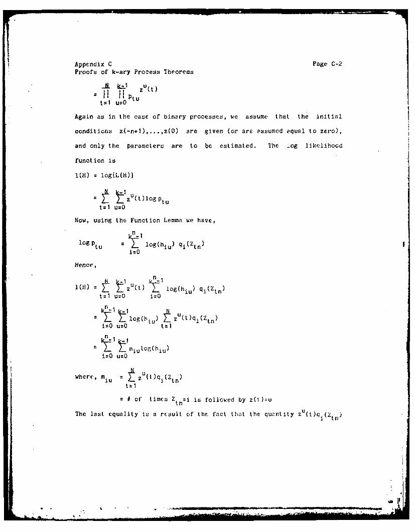
Appendix C Page C-2Proofs of k-ary Process Theorems
-ii iPtutW U=O
Again as in the case of binary processes, we assume that the initial
conditions z(-n+I),. .. ,z(O) are given (or are assumed equal to zero),
and only the parameters are to be estimated. The log likelihood
function is
1(IH) logtL(H))
t tI i zut)logp tut:I U=O
Now, using the Function Lemma we have,
logP~ p 1I og(hiu) qi(Ztn)i=O
H~ence,
- z uo(t~) , o~i U ) q (Ztn)
Wi O :O
ntThe lastg~ equlit ts acut of tefcn htte)aniyz tq(
ittn
of'~~~~~ times Z n s olwd yzt

Appendix C Page C-3Proofs of k-ary Process Theorems
is 1 if and only if z(t)zu, and Ztn=i" The maximum likelihood estimates
of the parameters are obtained by maximizing 1(H) under the constraints
hiu I i=0,1,...,kn- 1
uZO
We use the method of Lagrange multipliers for constrained maximization.
The modified objective function is
11(H) =kMiulog(hiu) + wi{ - / hiu }
i=0 uOO i=0 u=O
+ k I miulg(hiu)-Wihiu
i=O i=O u:O
Here wi are Lagarange multipliers. The necessary conditions for
maximization are
dl' miu
dhiu h - wi 0 , i=O,l,...,kn - I' u=O,1,...,k-1
iU iu
and hiu 1 t=0,1,...,k n -1
u=Omiu
The first equation above implies that hiu _w. The second equationi!
implies that
L u =i or wi miuiU=O u=-O
Therefore, the desired MLE of the parameters is
miuh iu Z I i=O,1,t ,kn ' 1 , uC0,1, .,k-1
uZO (Q.E.D. ]
- --. .

Appendix C Page C-4Proofs of k-ary Process Theorems
Proof of Predictioq Theorem : Let the desired estimate be
2(t) = g(Ztn )
where g is a Poolean function of Ztn. Again,
using the Lagrangean development of g we have,
kn=1(t) 1 g_ iq i(Ztn)
i=0
where ei is a k-ary variable given by e = g(Ztn!Ztni).
Applying the Function Lemma to the model and the predictor equation we
have
zU(t) = e()qi(Ztn)
i=0
v(t) = qi(Ztn)
i=O
and, therefore,
C(z(t)42(t)) = Cuv V(t)zU(t)
v=O u=O
n I 't f t~ vu,6e(t)qi(Z.n
i=O v=O u=O
or E[C(7(t),i(t))] = k._cuvhu
1=0 v=O u=O
= E[qi(Z td ) - -cuvhiu
i=O v=O u=0
The cost function is linear in . Obviously, should be so choson
' a
-...-

Appendix C Page C-5Proofs of k-ary Process Theorems
that the 91 that has the smallest coefficient is one (all other ev's
will then automatically become zero), i.e.,
ei arg min cuvhiu
u=O
NOW, if hiu is determined according to the Estimation Theorem, then hiu
is proportional to miu. Hence, the above formula for i is equivalent
to that stated in the theorem.
[Q.E.D.]
Proof of Corollary 4.8.4.1 : In this case, cuv 1 iff uv. Hence,
k-I
E cuvmiu = -Miv + tmiuu=O u=O
Hence, the v that maximizes miv also minimizes the left hand side of the
above equation and hence the cost function.
[Q.E.D.]
Proof of Total Cost Th rem
TC = C(z(t),z(t))t=1
- L~ L u(t)v(t)_ uvZ
t=1 v=O u:O
S . Cuv zu i Zt n )
t:1 i=O v:O u:O
i=O v=O u=O
V°-'.

Appendix C Page C-6Proofs of k-ary Process Theorems
= ) TCii=O
where IC. vtCuv i iuv=O u=O
=-- i L- CuvmiuV=O usO
min c M%, t- uviuu=O
The last equality is valid because e. is chosen according to thE
Prediction Theorem.
Hence, TC =Zlmintcuvmiu
L .F-:.D.
Prof orollary 4.8.5.1 This corollary follows straightfzrwardly
from the total cost theorem by substituting c U= iff uiv.
[QA...]

References Page R-1
[Aka74] H. Akaike, "A new look at the statistical model identification,"
IEEE Trans. on Automatic Control, vol. AC-19, no. 6, Dec 1974,
pp. 716-723.
[Arn75) C. R. Arnold, "A control theoretic approach to memory
management," Proceedings Ninth Asilmor Conference on Circuits,
Systems, and Computer, Pacific Grove, Calif., November 1975.
(Arn78] C. R. Arnold, "Optimization of computer operating systems,"
Ph. D. thesis, Harvard University, Cambridge, Mass., In
preparation.
[ArG74] C. R. Arnold and U. 0. Gapliardi, "A state-space formulation of
the resource allocation problem in computer operating systems,"
in Proc. 8th Asilmar Conf. on Circuits, Systems, Pnd
Computers, Pacific Grove, Calif., December 1974, pp. 713-722.
[Ash72] R. Ashany, "Application of control theory techniques to
performance analysis of computer systems," in Proc. 6th As!Imar
Conf. on Circuits, Systems, and Computers, Pacific Goove,
Calif., November 1972, pp. 90-101.
[Ast7O] K. J. Astrom, Utrodqct.Q to StochistiQ CQntg Th' r. New
York: Academic Press, 1970.
4

References Page R-2
[ADU71] A. V. Aho, P. J. Denning, and J. D. Ullman, "Principles of
optimal page replacement," JACM, vol. '8, no. 1, January 1971,
pp. 80-93.
(Bar46] M. S. Bartlett, "On the theoretical specification of the
sampling prop:rties of autocorrelated time series," Journal cf
the Royal Statistical Society, E8:27 1946.
(Be166] L. A. Belady, "A study of replacement algorithms for a virtual
storage computer," IBM Systems Journal, vol. 5, no. 2, 1965,
pp. 71-101.
(IR76] P. R. Blevins anf C. V. Hamamoorthy, "Aspects of a dynamicaliy
adaptive operating system," IEEE Trans. Comput., vol. C-2 ,
no. 7, July 1976, pp. 713-725.
[EoJ70] G. E. P. Pox and G. M. Jenkins, Time Series Anil sis Forr- stin
and Control. San Fransisco: Holden-Day Inc., 1970.
[BoP70] G. E. P. Box and D. A. Pierce, "Distribution cf residual
autocorrelation in autoregressive moving average time scries
models," Journal of the American StatisticnU Association 64,
1970.
[BrH69] A. E. Bryson, Jr. and Y. C. Ho, ApxLit, OpLimal Control.
Waltham, Mass: Ginn and Co., 1969.
AD-ATlSO392 HARVATI CAMRDEMUATIKN OFDPATIN LABEM RESUBC 9/2-TC
CDAI 92HRD NLTHERDRE DMAIN IFOPRATIN SYTES RESURC MA--T2U
MAY 7B B K JAIN N00914-76-C-0914UNCLASSIFIED TR-10-B NL3, 3 lllfE

32,
MICROCOPY RESOLUTION TEST CHARTNATIONAL BUREAU OF SIANDANDS-1963-A

References Page R-3
[Buz71] J. P. Buzen, "Queueing network models of multiprogramming,"
Ph. D. Thesis, Harvard University, Cambridge, Mass. 1971.
[BCB75] J. C. Browne, K. M. Chandy, et al, "Hierarchical techniques for
the development of realistic models of complex computer
systems," Proc. IEEE, vol. 63, no. 6, June 1975, pp. 966-975.
[BCM75] F. Baskett, K. M. Chandy, R. R. Muntz, and F. G. Palacios, "Open
closed and mixed networks of queues with different classes of
customers," JACM, vol. 22, no. 2, April 1975, pp. 248-260.
[Cle72] W. S. Cleveland, "The inverse autocorrelations of a time series
and their applications," Technometrics vol. 14 no. 2 May 1972,
pp. 277-293.
(Cof76] E. G. Coffman Jr., C jnd Job Shoo Schedling Theory.
John Wiley & Sons, 1976.
(Cou75] P. J. Courtois, "Decomposability, instabilities, and saturation
in multiprogramming systems," CACM, vol. 18, no. 7, July 1975,
Pp. 371-377.
(CoL66] D. R. Cox and P. A. W. Lewis, Ih jUtUtLLj= Analysis of .
Series of' Events. London: Methuen, 1966.
[CHW75] K. M. Chandy, U. Herzog, and L. Woo, "Approximate analysis of
general queueing networks," IBM J. Res. Develop., vol. 14,
no. 1, January 1975, pp. 43-49.

References Page R-4
[CMM67] R. W. Conway, W. L. Maxwell, and L. W. Miller, .TIhe. 2L
Schedullna. Reading, MA: Addision Wesley, 1967, pp. 27-30.
(Den68) P. J. Denning, "The working set model for program behavior,"
CACM, vol. 11, no. 5, May 1968, pp. 323-333.
[DKL76] P. J. Denning, K. C. Kahn, J. Leroudier, D. Potier, and R. Suri,
"Optimal Multiprogramming," Acta Informatica, vol. 7, fasc. 2,
1976, pp. 197-216.
(GaS73] D. P. Gaver and G. S. Shedler, "Approximate models for processor
utilization in multiprogrammed computer systems," SIAM J.
Comput., vol. 2, no. 3, September 1973, pp. 183-192.
(Gel75] E. Gelenbo, "On approximate computer systems models," JACM,
vol. 22, no. 2, April 1975, pp. 261-269.
(HaR68J P. L. Hammer (Ivanescu) and S. Rudeanu, E. tn _ tod.js inQ
Operations Research and Related Areas. New York:
Springer-Verlag, 1968.
[HoP72) C. A. R. Hoare and R. H. Pereot, OeratU.ng a vLii m I iq...
Pros. of International Seminar held at Oueen's University of
Belfast 1971, Academic Press 1972.
(Kas77] R. L. Kashyap, "A bayesian comparison of different classes of
dynamic models using empirical data," IEEE Trans. on Automatic
Control, vol. AC-22, no. 5, October 1977, pp. 715-727.
k!-

References Page R-5
(Kle69] L. Kleinrock, "Certain analytic results for time-shared
processors," in Information Processig 6U. A. J. H. Morrel,
Ed., Amsterdam: North-Holland Publishing Co., 1969,
pp. 838-845.
[Kle76] L. Kleinrock, Oueueing systms. vol. 2: Computer Applications,
ch. 4, New York: Wiley-Interscience, 1976.
[Lew74] A. Lew, "Optimal resource allocation and scheduling among
parallel processes," in Parallel Proesin. Tse-Yun Fung, Ed.,
Springer-Verlag, Berlin, 1974.
[Lew76] A. Lew, "Optimal control of demand-paging systems," Information
Sciences, vol. 10, no. 4, 1976, pp. 319-330.
(LiC77J L. Lipsky and J. D. Church, "Applications of a queueing network
model for a computer system," Computing Surveys, vol. 9, no. 3,
September 1977, pp. 205-221.
[MaD74) S. E. Madnick and J. J. Donovan, OperatinSjm. New York:
McGraw-Hill Book Co., 1974.
(McK69] J. M. McKinney, "A survey of analytical time-sharing models,"
Computing Surveys, vol. 1, no. 2, June 1969, pp. 105-116.
[(cW76] R. H. Mckeag and R. Wilson, tudie in QOUrIL=. m.
Academic Press 1976, Chapter 4.
I i-
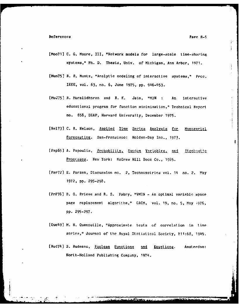
Refercnces Pare R-6
(Moo7l] C. G. Moore, III, "Network models for large-scale time-sharing
systems," Ph. D. Thesis, Univ. of Michigan, Ann Arbor, 1971.
(Mun75] R. R. Muntz, "Analytic modeling of interactive systems," Proc.
IEEE, vol. 63, no. 6, June 1975, pp. 946-953.
(MuJ751 R. Muralidharan and R. K. Jain, "MN An interactive
educational program for function minimization," Technical Report
no. 658, DEAP, Harvard University, December 1975.
[Ne1731 C. R. Nelson, Applied TiMe Series Analysis for Managerial
Foetastin&. San-Fransisco: Holden-Day Inc., 1973.
[Pap65] A. Papoulis, Probability Random Vriab]sle and Stoclnst i
Procsses. New York: McGraw Hill Book Co., 1965.
(Par72) E. Parzen, Discussion no. 2, Technometries vol. 14 no. 2. May
1972, pp. 295-298.
(PrF76] B. G. Prieve and R. S. Fabry, "VMIN - An optimal variable space
page replacement algorithm," CACM, vol. 19, no. 5, May i976,
pp. 295-297.
[Que49] M. H. Quenouille, "Approximate tests of correlation in time
series," Journal of the Royal Statistical Society, F11:68, 1949.
[Hud74] S. Rudeanu, _.Q(j E .u.aij jnd oUjtiQn. Amsterdam:
North-Holland Publishing Company, 1974.
A.

References Page R-7
(Sch67] A. Scherr, An AnalysIs of TimtShared Computer qX .
Research monograph 36, Cambridge, Mass.: M.I.T. Press, 1967.
[Shu76] A. W. C. Shum, "Queueing models for computer systems with
general service time distribution," Ph. D. Thesis, Harvard
University, Cambridge, Mass. Dec 1976.
(Smi56] W. E. Smith, "Various optimizations for single-stage
production," Naval Res. Logist. Quart., 3(1956) pp. 59-66.
[Smi78] D. R. Smith, "A new proof of the optimality of the shortest
remaining processing time discipline," Operations Research,
vol. 26, no. 1, Jan-Feb 1978, pp. 197-199.
(Wilt7] M. V. Wilkes, "Automatic load adjustment in time-sharing
systems," in Proc. ACM-SIGOPS workshop on System Performance
Evaluation, Harvard University, Cambridge, Mass. April 1971,
pp. 308-320.
[Wil73] M. V. Wilkes, "The dynamics of paging," Computer Journal,
vol. 16, no. 1, February 1973, pp. 4-9.
[Wul69] W. A. Wulf, "Performance monitors for multiprogramming systems,"
in Proc. 2nd Symp. on Operating Systems Principles, Princeton
Univ, October 1969, pp. 175-181.

ATE
LME