WRC RESEARCH REPORT NO. 54

HYDRAULIC GEOMETRY AND LOW STREAMFLOW REGIMEN

by

John B. Stall, Engineer

and

Chin Ted Yang, Assoc ia te Hyd ro log i s t

Illinois State Water Survey Urbanas Illinois

F I N A L R E P O R T

Pro jec t No. B-051-ILL

HYDRAULIC GEOMETRY AND LOW STREAMFLOW REGIMEN

Ju ly 1, 1970 - June 30, 1972

The work descr ibed in t h i s p u b l i c a t i o n was supported by matching funds of the I l l i n o i s State Water Survey and the U. S. Department of the I n t e r i o r , as au thor i zed under T i t l e 1 of the Water Resources Research

Act of 1964, P. L. 88-379

UNIVERSITY OF ILLINOIS WATER RESOURCES CENTER

2535 Hydrosystems Laboratory Urbana, I l l i n o i s 61801

Ju ly 1972

ABSTRACT

HYDRAULIC GEOMETRY AND LOW STREAMFLOW REGIMEN

Unit stream power defined as the time rate of potential energy expenditure per unit weight of water of a natural stream has been studied intensively in this report. It is shown that the distribution and variation of unit stream power have a determinate effect on the behavior of a natural stream. The unit stream power can be regulated by a stream through the combined process of meandering, forming pools and riffles, and carving a concave longitudinal stream bed profile. A study of the Kaskaskia River basin shows that sinuosity increases in the downstream direction by meandering. Field measurements made along the Middle Fork Vermilion River indicate that unit stream power can be minimized by the formation of pools and riffles. The hydraulic geometry--unit stream power equations developed for 9 river basins in the United States show that unit stream power in a river basin decreases with increasing frequency of flow and drainage area. These results are evidence of different levels of self adjustment made by a natural stream to minimize its unit stream power in accordance with the law of least time rate of energy expenditure. The calcu­lated dimensionless dispersion coefficients at 11 gaging stations in the Kaskaskia River Basin show that the coefficients increase with increasing width-depth ratio.

REFERENCE: Stall, John B., and Yang, Chih Ted, HYDRAULIC GEOMETRY AND LOW STREAMFLOW REGIMEN, University of Illinois Water Resources Center Research Report No. 54.

KEY WORDS: channels, dispersion, energy, hydraulic geometry, meanders, pools, riffles, stream systems, unit stream power

CONTENTS Page

Summary 1

I n t r o d u c t i o n 1

L i t e r a t u r e review 1

T i m e - o f - t r a v e l under r i f f l e - a n d - p o o l cond i t i ons . . . 2

Objec t ives 5

Acknowledgments 5

The concept of u n i t stream power 6

P o t e n t i a l energy and stream morphology 6

Long i tud ina l stream bed p r o f i l e 7

River meanders 8

R i f f l e s and pools 8

Bed forms 11

The heirarchy of unit stream power adjustments . . . . 11 Field measurements 11

Data collection 11 Results 12

The s t r u c t u r e of pools and r i f f l e s 16

The t e s t reach 17

Mapping methods 17

Results 19

Stream sinuosity 19 The test area 20 Methods 20 Results 21

Hydraulic geometry -- unit stream power equations 22 River curvature and shape 2k Dispersion in streams 25 Conclusion 28

Usefulness of results 28 References 30

HYDRAULIC GEOMETRY AND LOW STREAMFLOW REGIMEN

by John B. Stall and Chih Ted Yang

SUMMARY

Results of an investigation of unit stream power, defined as the time rate of potential energy expenditure per unit weight of water of a natural stream, are presented in this report. Theoretical studies and field investigations indicate that the distribution and variation of unit stream power have a determinate effect on the behavior of a natural stream. Therefore unit stream power can be regulated by a stream through the combined process of meandering, forming pools and riffles, and carving a concave longitudinal stream bed profile.

Hydraulic geometry—unit stream power equations are presented for 9 river basins in the United States. These equations show that unit stream power in a river basin decreases with increasing frequency of flow and drainage area.

It is the purpose of this report to provide a better understanding of the nature of stream systems with special emphasis on the principles of hydraulic geometry. Other aspects of this study include sinuousity, pools and riffles, and dispersion of a contaminant.

INTRODUCTION

Since 1895 the Illinois State Water Survey has carried out a full time program of research and evaluation of the water resources of Illinois including the quantity and quality of both surface waters and groundwaters. The project reported here is a part of this research and evaluation. In 1972 there were in Illinois about 160 continuous-record permanent stream gaging stations in opera­tion in Illinois. These gages are operated by the U.S. Geological Survey on a matching-funds basis in which half of the cost is paid by state or local sponsor­ing agencies. The data from these gaging stations have been used extensively in solving water resources problems in Illinois, and some of these data are used in this study.

Literature Review

An evaluation of the hydraulic geometry of Illinois streams was made in a study by Stall and Fok (1968). That study evaluated a consistent pattern in which the width, depth, and velocity of flow in a stream change along the course with a constant frequency of discharge. These channel characteristics, termed hydraulic geometry, were shown to constitute an interdependent system which was described by a series of graphs and equations. In a later study by Stall and

1

Yang (1970) similar sets of equations were provided for 12 selected river basins throughout the United States. These basins represented a much greater variety of physical conditions than the Illinois study. For all of these basins, however, the consistent patterns of hydraulic geometry were verified and equations were published.

The concept of hydraulic geometry was first published by Leopold and Maddock (1953). They suggested that channel characteristics of natural streams were interrelated in a complex manner, and showed how the nature of a particular river system could be described quantitatively. They first described this inter­related system as the hydraulic geometry of the stream system. Stall and Fok (1968) and Stall and Yang (1970) confirmed these general relationships and followed the general principles first suggested by Leopold and Maddock.

The nature and dynamics of a stream system have been described in a highly readable book by Morisawa (1968). A general description of channel conditions in major alluvial rivers has been provided by Fenwick (1969), and an excellent description of the hydraulic conditions in natural streams has been written by Posey (1950). A most thorough treatment of the hydraulics of open channel flow has been provided by Chow (1959). A new book on the hydraulics of sediment transport by Graf (1971) provides much information on flow conditions in channels.

According to Stall and Fok (1968) stream velocities computed from hydraulic geometry equations checked favorably with actual stream velocities measured by time-of-travel in streams determined by using dye tracers. These equations are used to compute the average depth and velocity of flow at problem locations on a stream where no measurements are available. The velocity equation was used to predict the time-of-travel for all principal Illinois streams (Stall and Hiestand, 1969). For that particular study, time-of-travel graphs were presented for 41 reaches of streams in Illinois showing the computed travel times at high, medium, and low flow conditions representing the flow occurring at a frequency of 10, 50, and 90 percent of the days per year. The computed travel times are most reliable at high flows, becoming less so at diminishing flow rates.

Time-of-Travel under Riffle-and-Pool Conditions

The dispersion of a contaminant within a stream is known to be associated with the stream hydraulics. Whenever a dye or contaminant is introduced into a stream in a relatively solid dose it is immediately subject to the turbulence in the stream caused by the various velocities present in the stream. As a conse­quence the contaminant is mixed or dispersed to some degree. It is well known that throughout the cross section of a stream there is considerable variation in the flow velocity. A small element of the stream flow at the top of the stream near the center has a considerably higher velocity than that which occurs deeper in the stream, near the stream bed, or at the sides along the stream banks. This difference means that the dye or contaminant will be carried downstream by the fastest moving element of the water and at the same time will begin to be dispersed throughout the cross section. After a period of time the dye will be carried by all elements of the stream water. This process of dis­persion will be discussed later in this report.

The measured time-of-travel at low flow rates is often much longer than that computed by equations. At low flows the water is held back by the pools and riffles when they exist in a stream bed. This phenomenon is illustrated in

2

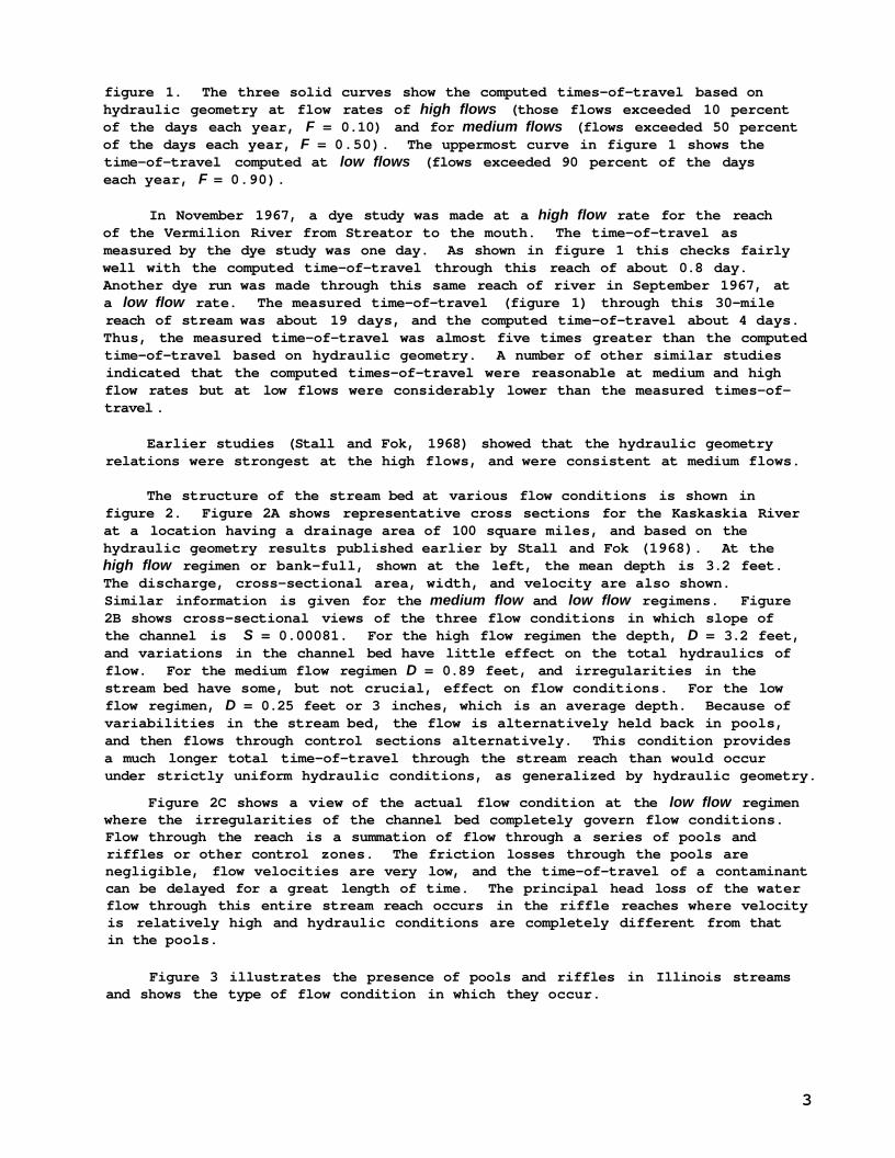
figure 1. The three solid curves show the computed times-of-travel based on hydraulic geometry at flow rates of high flows (those flows exceeded 10 percent of the days each year, F = 0.10) and for medium flows (flows exceeded 50 percent of the days each year, F = 0.50). The uppermost curve in figure 1 shows the time-of-travel computed at low flows (flows exceeded 90 percent of the days each year, F = 0.90).

In November 1967, a dye study was made at a high flow rate for the reach of the Vermilion River from Streator to the mouth. The time-of-travel as measured by the dye study was one day. As shown in figure 1 this checks fairly well with the computed time-of-travel through this reach of about 0.8 day. Another dye run was made through this same reach of river in September 1967, at a low flow rate. The measured time-of-travel (figure 1) through this 30-mile reach of stream was about 19 days, and the computed time-of-travel about 4 days. Thus, the measured time-of-travel was almost five times greater than the computed time-of-travel based on hydraulic geometry. A number of other similar studies indicated that the computed times-of-travel were reasonable at medium and high flow rates but at low flows were considerably lower than the measured times-of-travel .

Earlier studies (Stall and Fok, 1968) showed that the hydraulic geometry relations were strongest at the high flows, and were consistent at medium flows.

The structure of the stream bed at various flow conditions is shown in figure 2. Figure 2A shows representative cross sections for the Kaskaskia River at a location having a drainage area of 100 square miles, and based on the hydraulic geometry results published earlier by Stall and Fok (1968). At the high flow regimen or bank-full, shown at the left, the mean depth is 3.2 feet. The discharge, cross-sectional area, width, and velocity are also shown. Similar information is given for the medium flow and low flow regimens. Figure 2B shows cross-sectional views of the three flow conditions in which slope of the channel is S = 0.00081. For the high flow regimen the depth, D = 3.2 feet, and variations in the channel bed have little effect on the total hydraulics of flow. For the medium flow regimen D = 0.89 feet, and irregularities in the stream bed have some, but not crucial, effect on flow conditions. For the low flow regimen, D = 0.25 feet or 3 inches, which is an average depth. Because of variabilities in the stream bed, the flow is alternatively held back in pools, and then flows through control sections alternatively. This condition provides a much longer total time-of-travel through the stream reach than would occur under strictly uniform hydraulic conditions, as generalized by hydraulic geometry.

Figure 2C shows a view of the actual flow condition at the low flow regimen where the irregularities of the channel bed completely govern flow conditions. Flow through the reach is a summation of flow through a series of pools and riffles or other control zones. The friction losses through the pools are negligible, flow velocities are very low, and the time-of-travel of a contaminant can be delayed for a great length of time. The principal head loss of the water flow through this entire stream reach occurs in the riffle reaches where velocity is relatively high and hydraulic conditions are completely different from that in the pools.

Figure 3 illustrates the presence of pools and riffles in Illinois streams and shows the type of flow condition in which they occur.

3

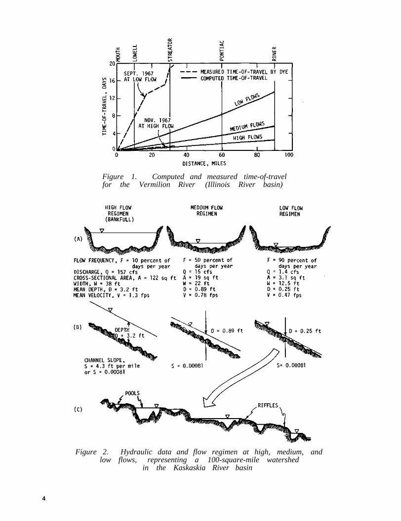
Figure 1. Computed and measured time-of-travel for the Vermilion River (Illinois River basin)

Figure 2. Hydraulic data and flow regimen at high, medium, and low flows, representing a 100-square-mile watershed

in the Kaskaskia River basin

4

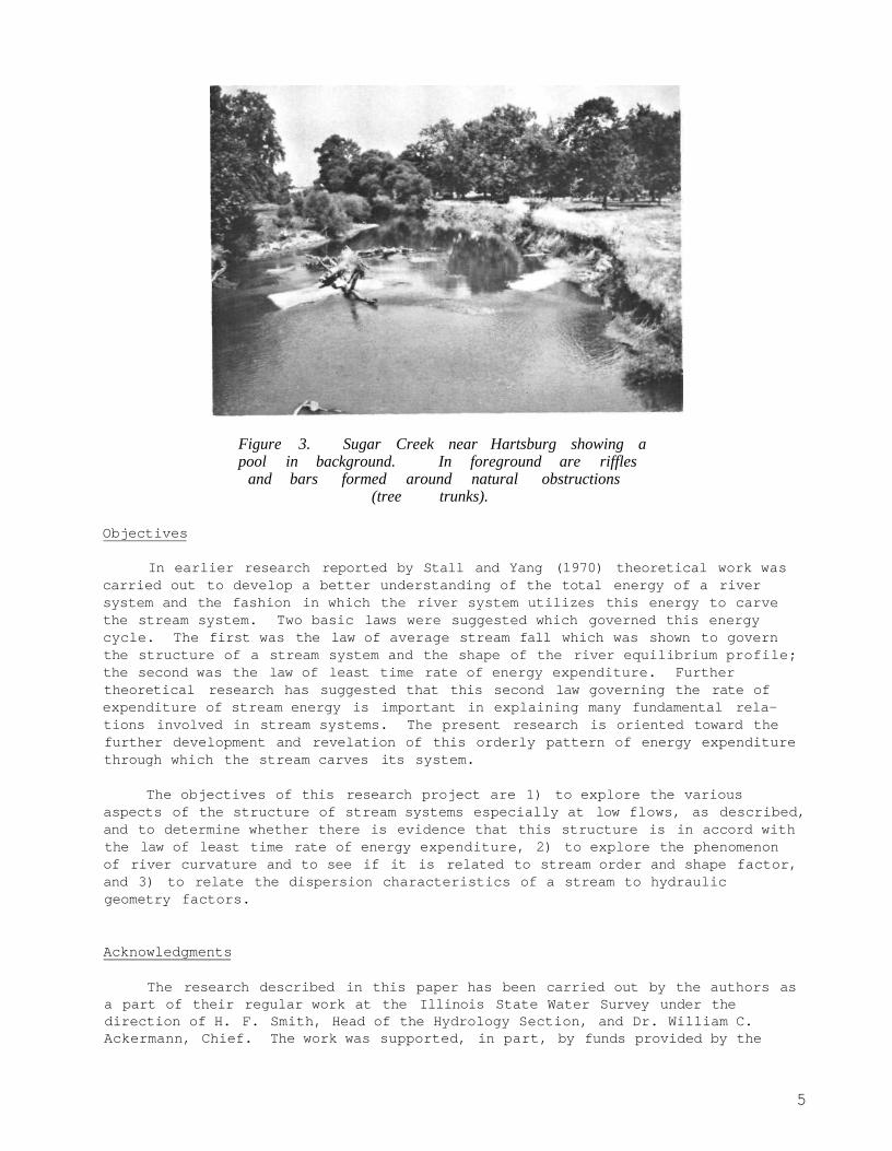
Figure 3. Sugar Creek near Hartsburg showing a pool in background. In foreground are riffles

and bars formed around natural obstructions (tree trunks).

Objectives

In earlier research reported by Stall and Yang (1970) theoretical work was carried out to develop a better understanding of the total energy of a river system and the fashion in which the river system utilizes this energy to carve the stream system. Two basic laws were suggested which governed this energy cycle. The first was the law of average stream fall which was shown to govern the structure of a stream system and the shape of the river equilibrium profile; the second was the law of least time rate of energy expenditure. Further theoretical research has suggested that this second law governing the rate of expenditure of stream energy is important in explaining many fundamental rela­tions involved in stream systems. The present research is oriented toward the further development and revelation of this orderly pattern of energy expenditure through which the stream carves its system.

The objectives of this research project are 1) to explore the various aspects of the structure of stream systems especially at low flows, as described, and to determine whether there is evidence that this structure is in accord with the law of least time rate of energy expenditure, 2) to explore the phenomenon of river curvature and to see if it is related to stream order and shape factor, and 3) to relate the dispersion characteristics of a stream to hydraulic geometry factors.

Acknowledgments

The research described in this paper has been carried out by the authors as a part of their regular work at the Illinois State Water Survey under the direction of H. F. Smith, Head of the Hydrology Section, and Dr. William C. Ackermann, Chief. The work was supported, in part, by funds provided by the

5

United States Department of the Interior as authorized under the Water Resources Act of 1964, Public Law 88-379. Dr. Ben B. Ewing, Director of the Water Resources Center and Dr. Harry Wenzel, Acting Director during 1972, have both been helpful to the authors in carrying out and reporting these research results.

Several of the important ideas pursued in this research were originally suggested by Ronald T. McLaughlin, Director of Enwats, Cambridge, Massachusetts, who conferred with the authors regarding the hydraulic aspects of natural streams early in the conception of this project. The authors received help and advice from Thomas Maddock of the U.S. Geological Survey. Written comments and advice on various theoretical aspects of the research were received from Luna Leopold and Walter Langbein of the U.S. Geological Survey.

The authors were aided greatly by specific suggestions regarding field methodology made by Joseph David Camp, Hydrologist, District Office for Illinois, U.S. Geological Survey in Champaign. Mr. Camp participated in a field trip in which the Embarras River bed was examined at a number of locations, and he advised the authors as to the appropriate values of hydraulic roughness to be used in the Manning equations. The authors also acknowledge other specific help from personnel of the same office of the U.S. Geological Survey; Davis W. Ellis, District Chief, provided much cooperation. Two discharge measurements were made by Kent M. Ogata, Hydraulic Engineer, and one discharge measurement was made by Robert E. Rentschler of the same office.

The water surface profile computed for the 300-mile reach of the Embarras River as a part of this project was carried out using a computer program developed by the Hydrologic Engineering Center of the Crops of Engineers, U.S. Army, at Davis, California. This computer program was altered for use in this study by Robert A. Sinclair, System Analyst of the State Water Survey. Copies of 837 cross sections on the Embarras River were provided to the project by the Division of Waterways, Illinois Department of Transportation.

Illustrations for the report were done by John W. Brother, Jr., and the report was edited by Patricia A. Motherway, Assistant Technical Editor, both of the State Water Survey. Engineering assistants who worked part time on this project while students at the University of Illinois in Civil Engineering were Dr. Y. C. Yoon, John Gulledge, Jahangir Azma, Y. Y. Shen, and Michael MacLiesh.

The field survey work on the Vermilion River was aided greatly by the help of Fay G. Juvinall, Park Ranger at Kickapoo State Park, Illinois Department of Conservation. Other Park personnel were helpful also.

THE CONCEPT OF UNIT STREAM POWER

Potential Energy and Stream Morphology

The concept of entropy was introduced to the evaluation of stream morphol­ogy by Leopold and Langbein (1962). Scheidegger (1964) showed the existence of the basic analogy between absolute temperature of a thermal system and elevation of a stream system. By using the analogy that the absolute temperature and thermal energy in a thermal system is equivalent to the elevation and potential energy in a stream system, Yang (1971a) derived two basic laws in stream mor­phology. The law of average stream fall states that for any river basin that

6

has reached its dynamic equilibrium condition, the ratio of the average fall between any two different order streams in the same river basin is unity. The law of least time rate of energy expenditure states that during the evolution toward its equilibrium condition, a natural stream chooses its course of flow in such a manner that the time rate of potential energy expenditure per unit mass or weight of water along this course is a minimum. This minimum value depends on the external constraints applied to the stream. The law of average stream fall was used by Stall and Yang (1970), Yang (1971a), and Yang and Stall (1971) for the calculation of equilibrium stream bed profiles. The present report explores the further confirmation of the law of least time rate of energy expen­diture.

Longitudinal Stream Bed Profile

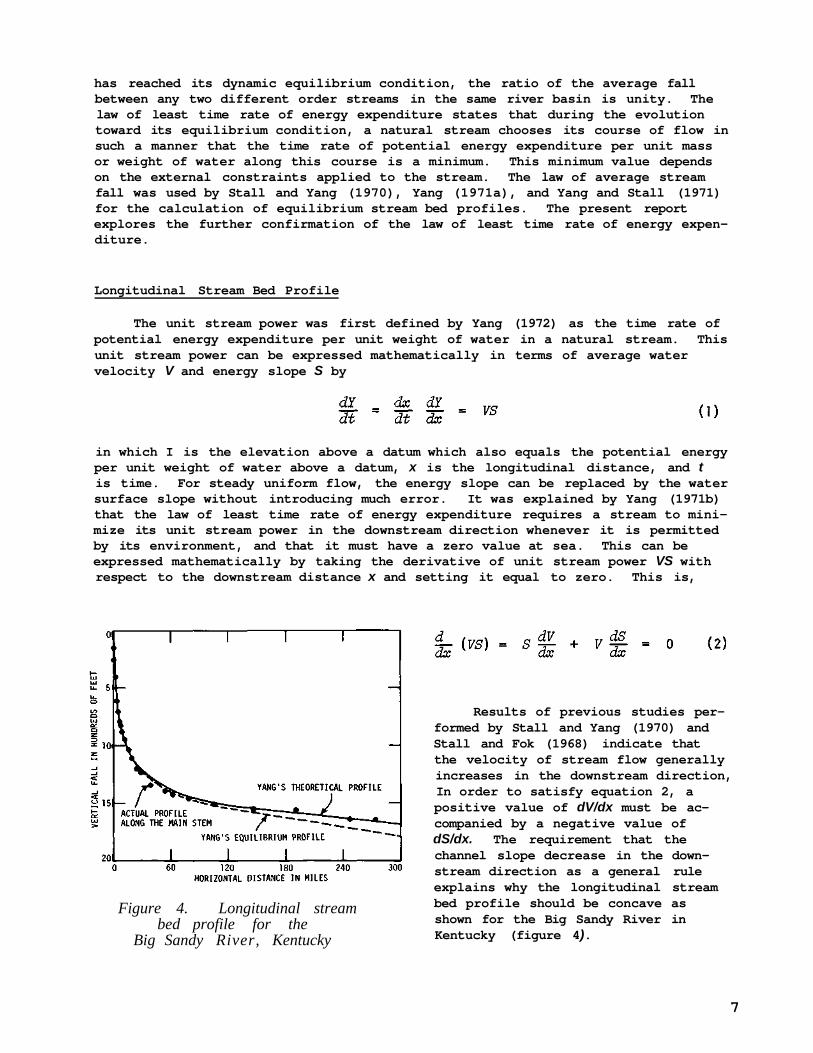
The unit stream power was first defined by Yang (1972) as the time rate of potential energy expenditure per unit weight of water in a natural stream. This unit stream power can be expressed mathematically in terms of average water velocity V and energy slope S by

Figure 4. Longitudinal stream bed profile for the

Big Sandy River, Kentucky

Results of previous studies per­formed by Stall and Yang (1970) and Stall and Fok (1968) indicate that the velocity of stream flow generally increases in the downstream direction, In order to satisfy equation 2, a positive value of dV/dx must be ac­companied by a negative value of dS/dx. The requirement that the channel slope decrease in the down­stream direction as a general rule explains why the longitudinal stream bed profile should be concave as shown for the Big Sandy River in Kentucky (figure 4).

7

in which I is the elevation above a datum which also equals the potential energy per unit weight of water above a datum, x is the longitudinal distance, and t is time. For steady uniform flow, the energy slope can be replaced by the water surface slope without introducing much error. It was explained by Yang (1971b) that the law of least time rate of energy expenditure requires a stream to mini­mize its unit stream power in the downstream direction whenever it is permitted by its environment, and that it must have a zero value at sea. This can be expressed mathematically by taking the derivative of unit stream power VS with respect to the downstream distance x and setting it equal to zero. This is,

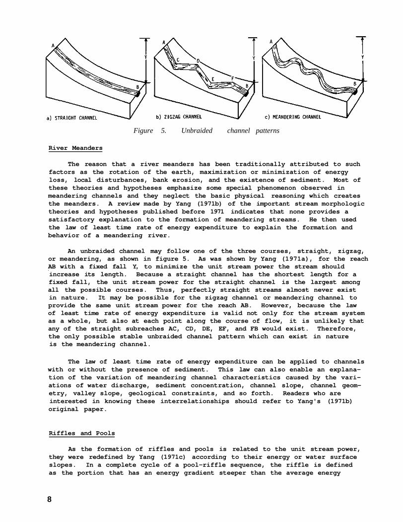
Figure 5. Unbraided channel patterns

River Meanders

The reason that a river meanders has been traditionally attributed to such factors as the rotation of the earth, maximization or minimization of energy loss, local disturbances, bank erosion, and the existence of sediment. Most of these theories and hypotheses emphasize some special phenomenon observed in meandering channels and they neglect the basic physical reasoning which creates the meanders. A review made by Yang (1971b) of the important stream morphologic theories and hypotheses published before 1971 indicates that none provides a satisfactory explanation to the formation of meandering streams. He then used the law of least time rate of energy expenditure to explain the formation and behavior of a meandering river.

An unbraided channel may follow one of the three courses, straight, zigzag, or meandering, as shown in figure 5. As was shown by Yang (1971a), for the reach AB with a fixed fall Y, to minimize the unit stream power the stream should increase its length. Because a straight channel has the shortest length for a fixed fall, the unit stream power for the straight channel is the largest among all the possible courses. Thus, perfectly straight streams almost never exist in nature. It may be possible for the zigzag channel or meandering channel to provide the same unit stream power for the reach AB. However, because the law of least time rate of energy expenditure is valid not only for the stream system as a whole, but also at each point along the course of flow, it is unlikely that any of the straight subreaches AC, CD, DE, EF, and FB would exist. Therefore, the only possible stable unbraided channel pattern which can exist in nature is the meandering channel.

The law of least time rate of energy expenditure can be applied to channels with or without the presence of sediment. This law can also enable an explana­tion of the variation of meandering channel characteristics caused by the vari­ations of water discharge, sediment concentration, channel slope, channel geom­etry, valley slope, geological constraints, and so forth. Readers who are interested in knowing these interrelationships should refer to Yang's (1971b) original paper.

Riffles and Pools

As the formation of riffles and pools is related to the unit stream power, they were redefined by Yang (1971c) according to their energy or water surface slopes. In a complete cycle of a pool-riffle sequence, the riffle is defined as the portion that has an energy gradient steeper than the average energy

8

gradient of the complete cycle, whereas the pool is the portion that has an energy gradient milder than the cycle average.

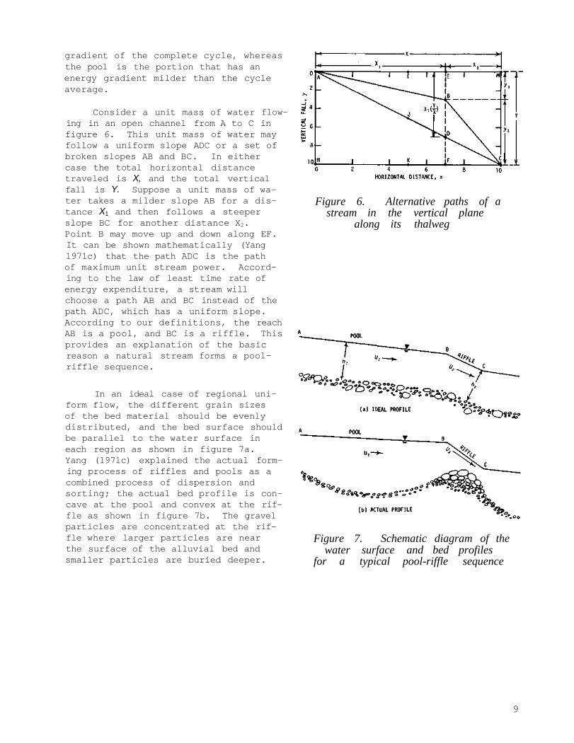
Consider a unit mass of water flow­ing in an open channel from A to C in figure 6. This unit mass of water may follow a uniform slope ADC or a set of broken slopes AB and BC. In either case the total horizontal distance traveled is X, and the total vertical fall is Y. Suppose a unit mass of wa­ter takes a milder slope AB for a dis­tance X1 and then follows a steeper slope BC for another distance X2. Point B may move up and down along EF. It can be shown mathematically (Yang 1971c) that the path ADC is the path of maximum unit stream power. Accord­ing to the law of least time rate of energy expenditure, a stream will choose a path AB and BC instead of the path ADC, which has a uniform slope. According to our definitions, the reach AB is a pool, and BC is a riffle. This provides an explanation of the basic reason a natural stream forms a pool-riffle sequence.

In an ideal case of regional uni­form flow, the different grain sizes of the bed material should be evenly distributed, and the bed surface should be parallel to the water surface in each region as shown in figure 7a. Yang (1971c) explained the actual form­ing process of riffles and pools as a combined process of dispersion and sorting; the actual bed profile is con­cave at the pool and convex at the rif­fle as shown in figure 7b. The gravel particles are concentrated at the rif­fle where larger particles are near the surface of the alluvial bed and smaller particles are buried deeper.

Figure 6. Alternative paths of a stream in the vertical plane

along its thalweg

Figure 7. Schematic diagram of the water surface and bed profiles

for a typical pool-riffle sequence

9

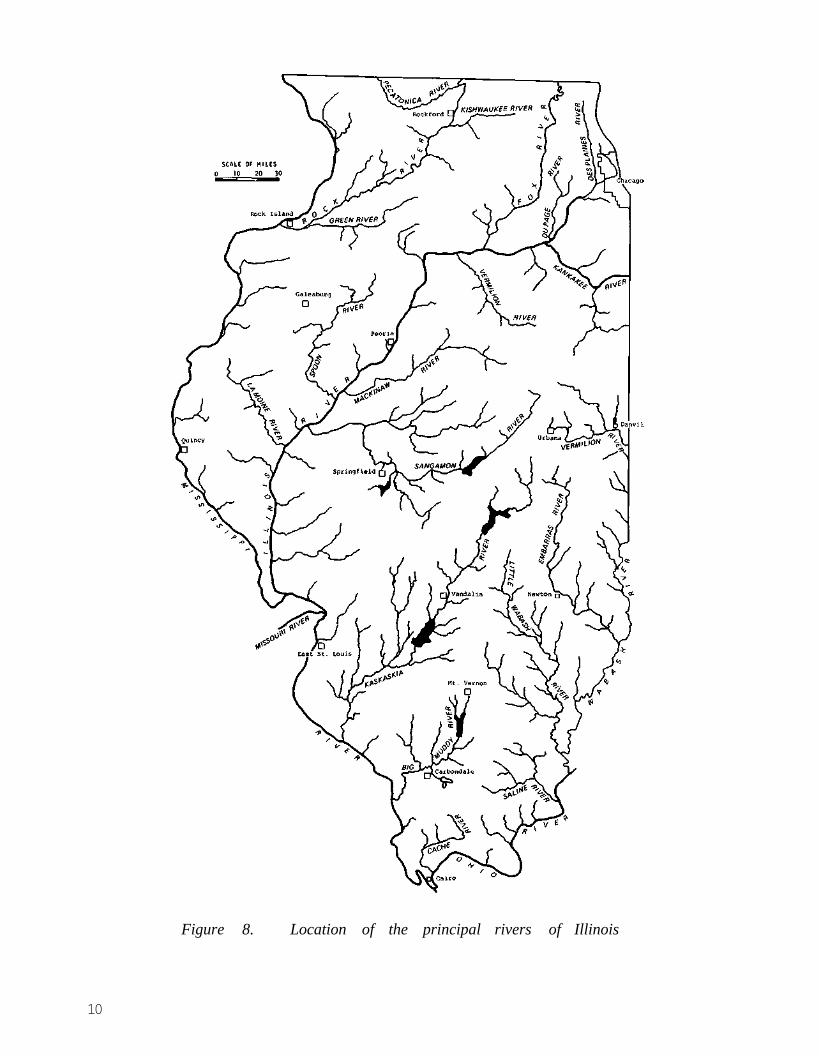
Figure 8. Location of the principal rivers of Illinois

10

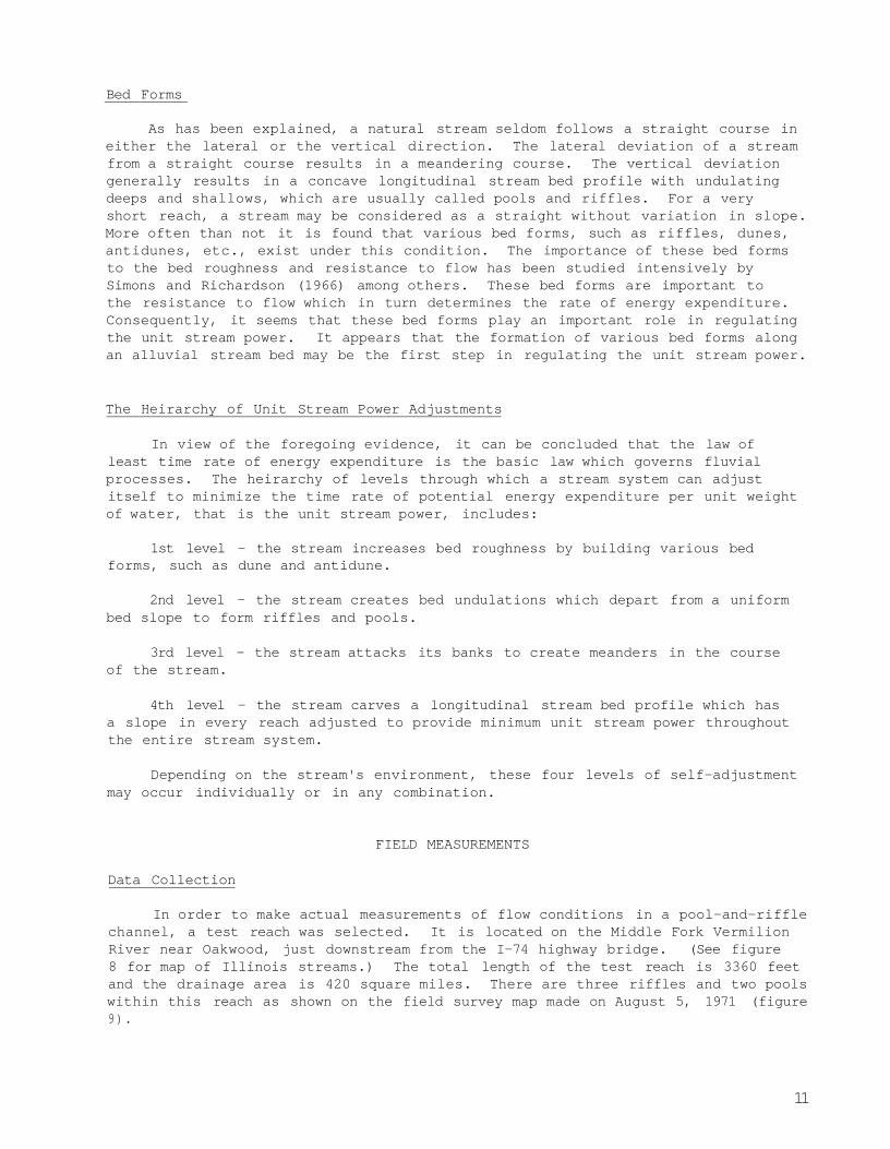
Bed Forms

As has been explained, a natural stream seldom follows a straight course in either the lateral or the vertical direction. The lateral deviation of a stream from a straight course results in a meandering course. The vertical deviation generally results in a concave longitudinal stream bed profile with undulating deeps and shallows, which are usually called pools and riffles. For a very short reach, a stream may be considered as a straight without variation in slope. More often than not it is found that various bed forms, such as riffles, dunes, antidunes, etc., exist under this condition. The importance of these bed forms to the bed roughness and resistance to flow has been studied intensively by Simons and Richardson (1966) among others. These bed forms are important to the resistance to flow which in turn determines the rate of energy expenditure. Consequently, it seems that these bed forms play an important role in regulating the unit stream power. It appears that the formation of various bed forms along an alluvial stream bed may be the first step in regulating the unit stream power.

The Heirarchy of Unit Stream Power Adjustments

In view of the foregoing evidence, it can be concluded that the law of least time rate of energy expenditure is the basic law which governs fluvial processes. The heirarchy of levels through which a stream system can adjust itself to minimize the time rate of potential energy expenditure per unit weight of water, that is the unit stream power, includes:

1st level - the stream increases bed roughness by building various bed forms, such as dune and antidune.

2nd level - the stream creates bed undulations which depart from a uniform bed slope to form riffles and pools.

3rd level - the stream attacks its banks to create meanders in the course of the stream.

4th level - the stream carves a longitudinal stream bed profile which has a slope in every reach adjusted to provide minimum unit stream power throughout the entire stream system.

Depending on the stream's environment, these four levels of self-adjustment may occur individually or in any combination.

FIELD MEASUREMENTS

Data Collection

In order to make actual measurements of flow conditions in a pool-and-riffle channel, a test reach was selected. It is located on the Middle Fork Vermilion River near Oakwood, just downstream from the I-74 highway bridge. (See figure 8 for map of Illinois streams.) The total length of the test reach is 3360 feet and the drainage area is 420 square miles. There are three riffles and two pools within this reach as shown on the field survey map made on August 5, 1971 (figure 9).

11

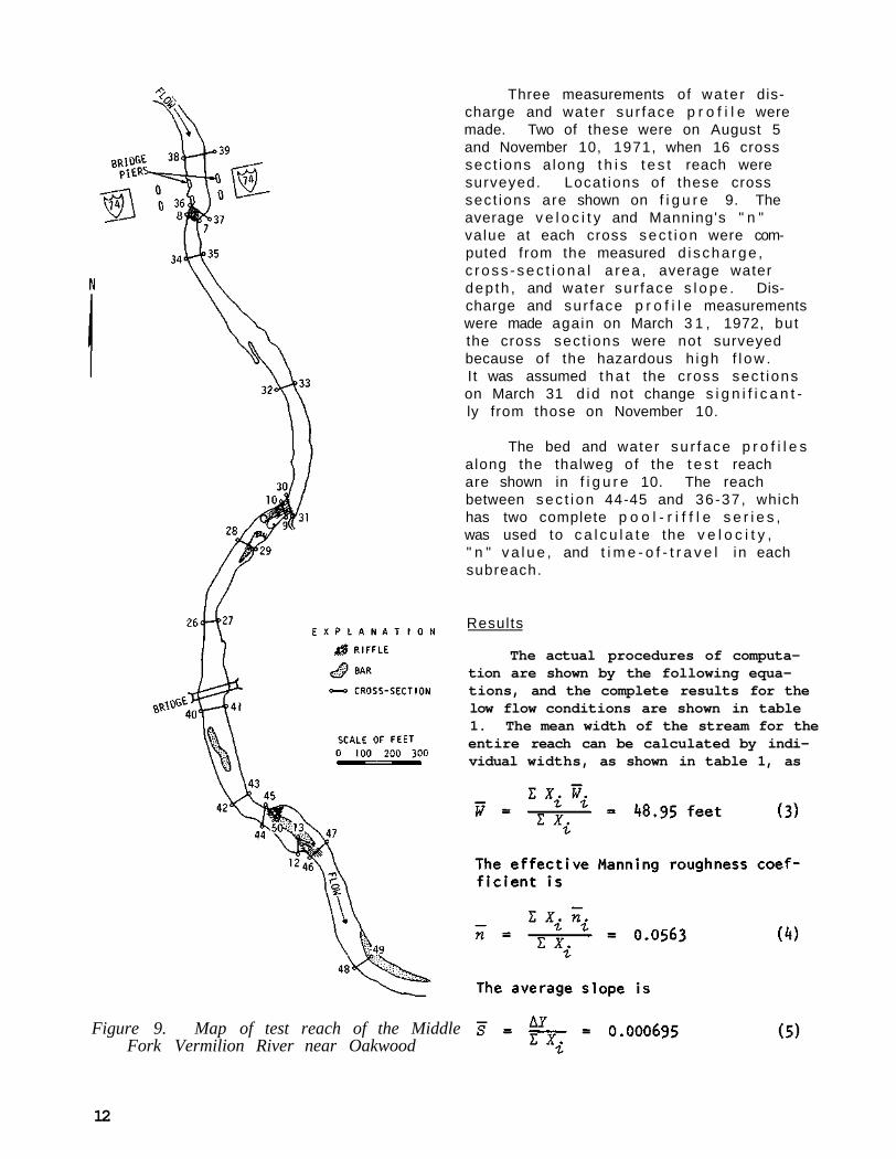
Figure 9. Map of test reach of the Middle Fork Vermilion River near Oakwood

Three measurements of wate r dis­charge and water sur face p r o f i l e were made. Two of these were on August 5 and November 10, 1971, when 16 cross sec t ions a long t h i s t e s t reach were surveyed. Locat ions of these cross sect ions are shown on f i g u r e 9. The average v e l o c i t y and Manning's " n " value at each cross sec t i on were com­puted from the measured d i scha rge , c r o s s - s e c t i o n a l a rea , average water dep th , and water sur face s l o p e . Dis­charge and sur face p r o f i l e measurements were made again on March 3 1 , 1972, but the cross sec t ions were not surveyed because of the hazardous h igh f l o w . It was assumed t ha t the cross sec t ions on March 31 d id not change s i g n i f i c a n t ­ly from those on November 10.

The bed and water su r face p r o f i l e s along the thalweg of the t e s t reach are shown in f i g u r e 10. The reach between sec t i on 44-45 and 36-37, which has two complete p o o l - r i f f l e s e r i e s , was used to c a l c u l a t e the v e l o c i t y , " n " v a l u e , and t i m e - o f - t r a v e l in each subreach.

Results

The actual procedures of computa­tion are shown by the following equa­tions, and the complete results for the low flow conditions are shown in table 1. The mean width of the stream for the entire reach can be calculated by indi­vidual widths, as shown in table 1, as

12

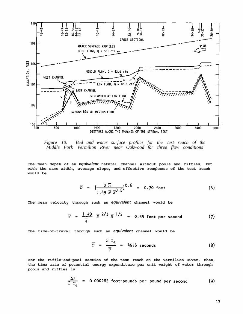
Figure 10. Bed and water surface profiles for the test reach of the Middle Fork Vermilion River near Oakwood for three flow conditions

The mean depth of an equivalent natural channel without pools and riffles, but with the same width, average slope, and effective roughness of the test reach would be

The mean velocity through such an equivalent channel would be

The time-of-travel through such an equivalent channel would be

For the riffle-and-pool section of the test reach on the Vermilion River, then, the time rate of potential energy expenditure per unit weight of water through pools and riffles is

13

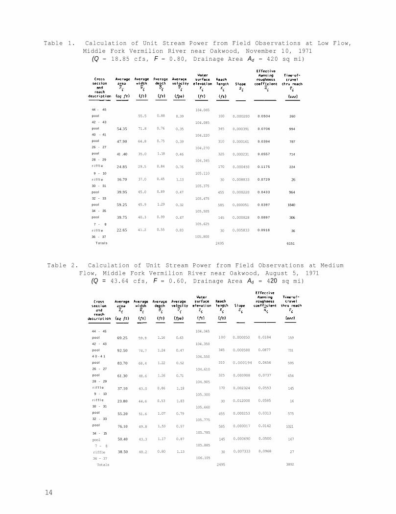
Table 1. Calculation of Unit Stream Power from Field Observations at Low Flow, Middle Fork Vermilion River near Oakwood, November 10, 1971

(Q = 18.85 cfs, F = 0.80, Drainage Area Ad = 420 sq mi)

Table 2. Calculation of Unit Stream Power from Field Observations at Medium Flow, Middle Fork Vermilion River near Oakwood, August 5, 1971

(Q = 43.64 cfs, F = 0.60, Drainage Area Ad = 420 sq mi)

14

44 - 45

pool

42 - 43

pool

40 - 41

pool

26 - 27

pool

28 - 29

r i f f l e

9 - 10

r i f f l e

30 - 31

pool

32 - 33

pool

34 - 35

pool

7 - 8

r i f f l e

36 - 37

T o t a l s

54.35

47.90

41 .40

24.85

16.70

39.95

59.25

39.75

22.65

55.5

71.8

64.8

35.0

29.5

37.0

45.0

45.9

40.3

41.2

0.88

0.76

0.75

1.18

0.84

0.45

0.89

1.29

0.99

0.55

0.39

0.35

0.39

0.46

0.76

1.13

0.47

0.32

0.47

0.83

104.065

104.085

104.220

104.270

104.345

105.110

105.375

105.475

105.505

105.625

105.800

100

345

310

325

170

30

455

585

145

30

2495

0.000200

0.000391

0.000161

0.000231

0.000450

0.008833

0.000220

0.000051

0.000828

0.005833

0.0504

0 .0706

0.0394

0.0557

0 .1175

0 .0729

0 .0433

0 .0397

0 .0897

0.0918

260

994

787

714

224

26

964

1840

306

36

6151

44 - 45

pool

42 - 43

poo l

4 0 - 4 1

poo l

26 - 27

pool

28 - 29

r i f f l e

9 - 10

r i f f l e

30 - 31

pool

32 - 33

pool

34 - 15

pool 7 - 8 riffle 36 - 37 Totals

69.25

92.50

83.70

61.30

37.10

23.80

55.20

76.10

50.40

38.50

59.9

74.7

68.4

48.6

43.0

44.6

51.6

49.8

43.3

48.2

1.16

1.24

1.22

1.26

0.86

0.53

1.07

1.53

1.17

0.80

0.63

0.47

0.52

0.71

1.18

1.83

0.79

0.57

0.87

1.13

104.345

104.350

104.550

104.610

104.905

105.300

105.660

105.775

105.785

105.885

106.105

100

345

310

325

170

30

455

585

145

30

2495

0.000050

0.000580

0.000194

0.000908

0.002324

0.012000

0.000253

0.000017

0.000690

0.007333

0.0184

0.0877

0.0456

0.0737

0.0553

0.0585

0.0313

0.0142

0.0500

0.0968

159

731

595

456

145

16

575

1021

167

27

3892

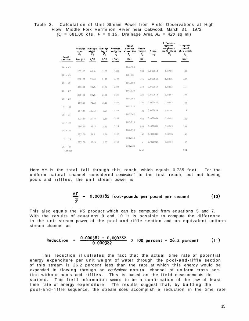
Here ∆Y is the t o t a l f a l l through t h i s reach, which equals 0.735 f o o t . For the un i form na tu ra l channel considered equivalent to the t e s t reach, but not having pools and r i f f l e s , the u n i t stream power is

This a lso equals the VS product which can be computed from equat ions 5 and 7. With the r e s u l t s of equat ions 9 and 10 it is poss ib le to compute the d i f f e r e n c e in the u n i t stream power of the p o o l - a n d - r i f f l e sec t i on and an equ iva len t un i fo rm stream channel as

This reduct ion i l l u s t r a t e s the f a c t tha t the ac tua l t ime ra te o f p o t e n t i a l energy expend i tu re per u n i t we ight o f water through the p o o l - a n d - r i f f l e sec t i on of t h i s stream is 26.2 percent less than the ra te at which t h i s energy would be expended in f l ow ing through an equivalent na tu ra l channel of un i form cross sec­t i o n w i t hou t pools and r i f f l e s . This is based on the f i e l d measurements de­s c r i b e d . This f i e l d i n fo rma t ion seems to be a con f i rma t i on of the law of leas t t ime ra te of energy expend i t u re . The resu l t s suggest t h a t , by b u i l d i n g the p o o l - a n d - r i f f l e sequence, the stream does accomplish a reduc t ion in the t ime ra te

15

Table 3. C a l c u l a t i o n of Un i t Stream Power f rom F ie l d Observat ions at High Flow, Middle Fork Vermi l ion River near Oakwood, March 3 1 , 1972

(Q = 681.00 c f s , F = 0 .15, Drainage Area Ad = 420 sq mi)

44 - 45

42 - 43

40 - 41

26 - 27

28 - 29

9 - 10

30 - 31

32 - 33

34 - 35

7 - 8

36 - 37 Totals

207.50

250.00

243.00

208.90

198.80

197.50

202.10

216.30

217.30

217.60

80.8

91.8

95.5

80.5

92.2

120.2

107.5

89.7

95.4

110.5

2.57

2.72

2.54

2.60

2.16

1.64

1.88

2.41

2.28

1.97

3.28

2.72

2.80

3.25

3.42

3.44

3.37

3.14

3.13

3.13

106.300

106.380

106.660

106.910

107.180

107.320

107.340

107.710

108.190

108.310

108.330

100

345

310

325

170

30

455

585

145

30

2495

0.000814

0.000814

0.000814

0.000814

0.000814

0.000814

0.000814

0.000814

0.000814

0.000814

0.0243

0.0305

0.0283

0.0247

0.0207

0.0171

0.0192

0.0243

0.0235

0.0214

30

127

III

100

50

9

135

186

46

10

804

of expenditure of its potential energy.

Table 2 gives similar calculations based on field measurements taken August 5, 1971, at a flow frequency of F = 0.60, or during a medium flow condi­tion. Table 3 gives calculations based on field measurements taken on March 31, 1972, at a flow frequency of F = 0.15, a high flow condition. For this condi­tion the pools and riffles were obscured and the water surface profile through the entire test reach was virtually straight, with uniform slope.

Table 4. Unit Stream Power Results for Three Flow Conditions, Middle Fork Vermilion River near Oakwood

Unit Stream Power (foot-pounds per pound per second)

Flow amount

Q (cfs)

18.9 43.6 681

frequency F

(% of days)

0.80 0.60 0.15

through pools and

riffles

0.000282 0.000452 0.002526

through uni form

equivalent channel

0.000382 0.000589 0.002522

reduction %

26.2 23.3 0

In table 4 the results are shown for all three of the field measurements. At low and medium flows the unit stream power was reduced by 26.2 and 23.3 percent, respectively, by the presence of the pools and riffles. At the high flows the pools and riffles were obscured by the deep depth of water and had no effect on the unit stream power. This result adds to the validity of the results at low and medium flows because in these cases an equivalent uniform natural channel condition was used to compare with the pool-and-riffle condition. The high flow condition illustrates that, for the condition where riffles and pools are obscured or effectively do not exist, the unit stream power can be reasonably computed by the methods used here. This is the condition in uniform natural channels. Consequently the computed reduction in unit stream power in the pool and riffle channel is a valid reduction from that which would occur in the natural channel without the pools and riffles.

Tables 1, 2, and 3 show that the water surface slope S in an equivalent natural channel is 0.000695 for the low flow and 0.000705 for medium flow. This is an extremely small difference; the slope is almost the same for both condi­tions. The slope is only slightly higher, 0.000814 for the high flow. The effective Manning roughness coefficient values shown in tables 1, 2, and 3 are highly variable which illustrates the wide range of the hydraulic conditions which actually prevail within the various sections of a pool-and-riffle channel.

THE STRUCTURE OF POOLS AND RIFFLES

As part of this field study a reach of the Kaskaskia River downstream from Vandalia (see figure 8) was selected as being representative of the pool-and-

16

riffle condition in combination with excessive meandering. A field inspection trip was made by boat along a 6.7 mile reach of the stream on September 1, 1970. On that date the flow was Q = 47 cfs, a flow which has a frequency of F = 0.89. At that time the stream bed consisted of a series of pools and riffles, and tree trunks and other debris caused natural obstructions to the stream flow. It was noted that the stream took advantage of each natural obstruction to build up a gravel bar and create a riffle condition.

The Test Reach

In order to generalize the structure, size, and configuration of pools and riffles a study was made of the Kaskaskia River for a distance of 53 miles up­stream from Vandalia. High quality aerial photographs of this reach which were taken on September 16, 1953 were available. On this date the flow in the stream was Q = 22 cfs, which has a flow frequency of F = 0.97. These aerial photographs were taken by the U.S. Department of Agriculture and a complete set was available from the Map Library of the University of Illinois. On these photographs the river course was easily discernable; meanders and the pools and riffles could be seen readily. For the purpose of this study a special set of 13 photographs having a scale of 8 inches to the mile was purchased. Inspection of these aerial photographs made it possible to map the location of all of the riffles and pools in this 53_mile section of the Kaskaskia River (see figure 11). For example, a riffle condition is found between sections 11 and 12; a pool condition is found between sections 12 and 13; a riffle exists between sections 13 and 14; and a pool exists between sections 14 and 15, and so forth.

Mapping Methods

In inspecting these aerial photographs it was necessary to utilize consid­erable judgment in designating the riffle condition and the pool condition within the river. Light reflection on the water surface was sometimes confusing; but in general it was possible to designate the actual presence of a riffle condition as differentiated from a light reflection. It was also found that the width of the river in the riffle section could be measured from the aerial photo­graph most accurately. Often for the pool condition it was not possible to obtain an accurate measurement of the width of the river because of the presence of overhanging trees and leaves which obscured the exact river edge.

Certain other mapping problems limited the delineation of pools and riffles and caused some pools and riffles to be excluded from the final analysis of this study.

First, those pools which had more than one bend, such as the reach between sections 6 and 7 in figure 11, were not included in the analysis because, accord­ing to Yang (1971c), the existence of a riffle depends on the stage of water. A riffle may show up near the point of inflection along the course between sections 6 and 7 at a lower stage. Secondly, reaches which are fairly straight, such as the reach between sections 20 and 23 were also excluded from analysis because a reasonable measurement of the length of riffle was impossible. Thus only those pools such as 2 to 3 and 4 to 5 and their immediate downstream riffles 1 to 2 and 3 to 4 were included in this analysis.

17

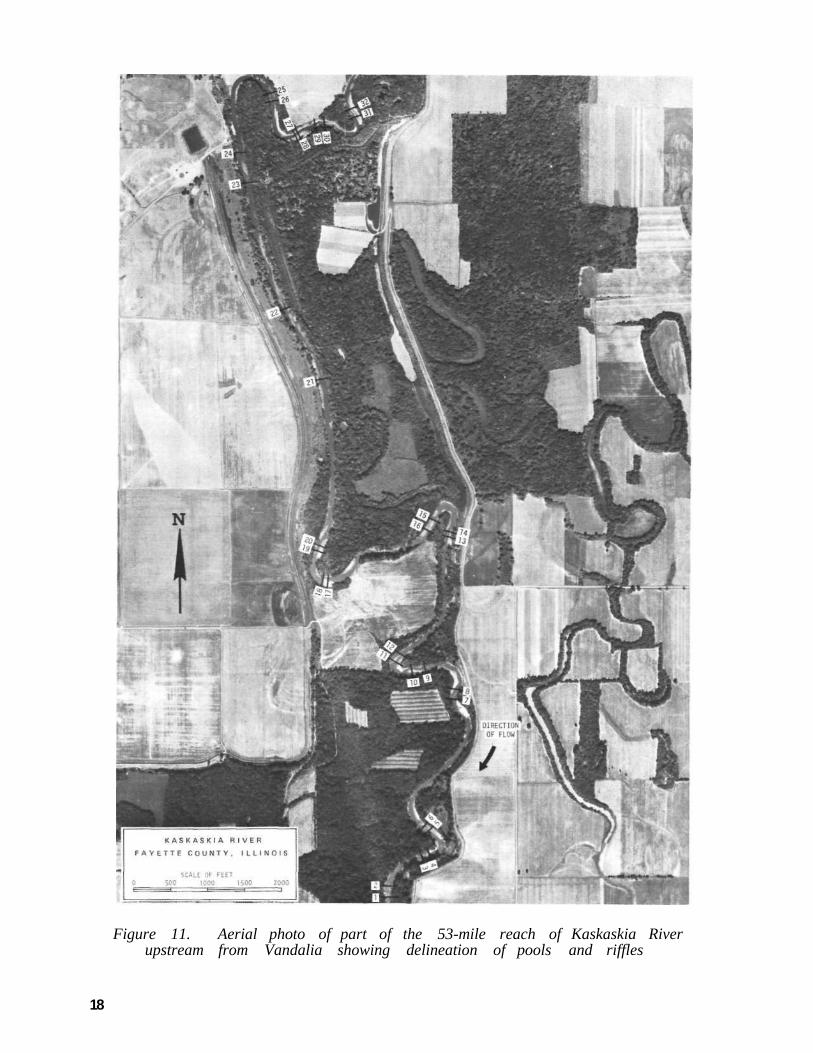
Figure 11. Aerial photo of part of the 53-mile reach of Kaskaskia River upstream from Vandalia showing delineation of pools and riffles

18

Results

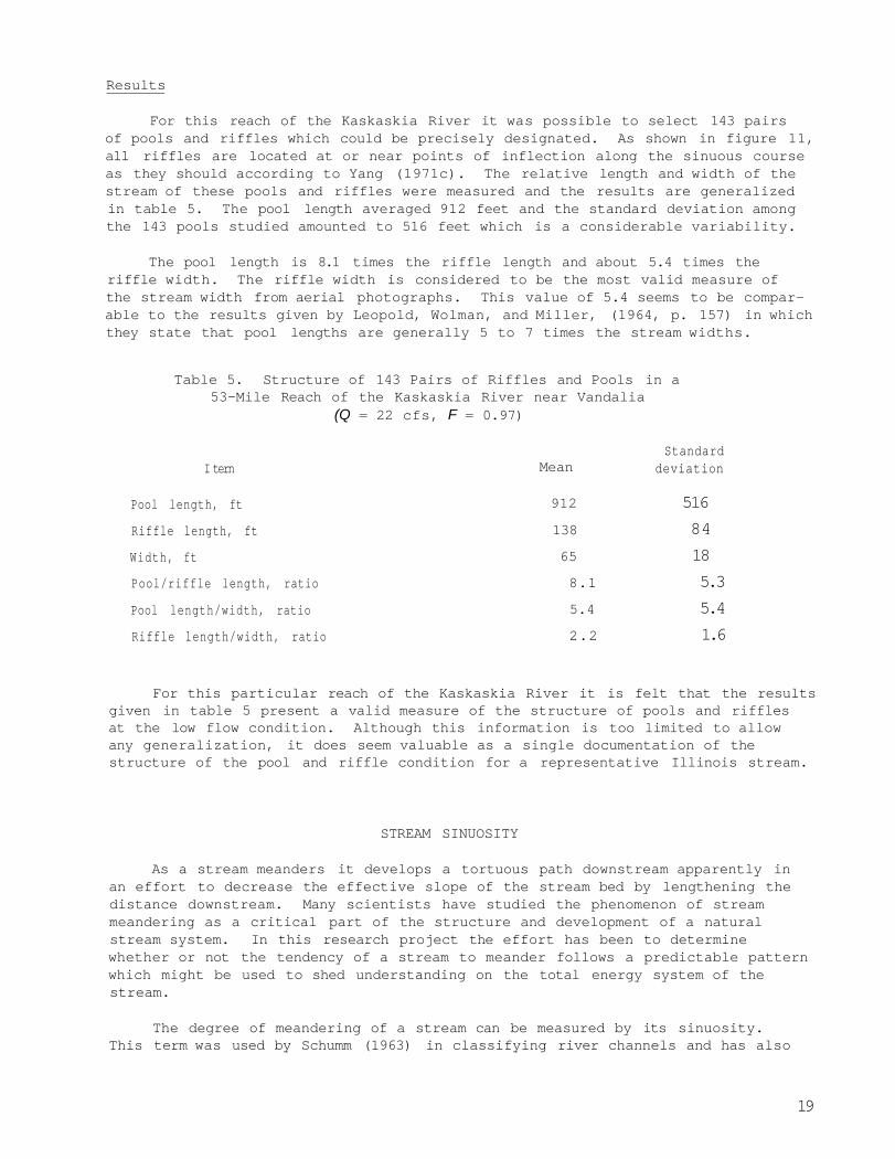
For this reach of the Kaskaskia River it was possible to select 143 pairs of pools and riffles which could be precisely designated. As shown in figure 11, all riffles are located at or near points of inflection along the sinuous course as they should according to Yang (1971c). The relative length and width of the stream of these pools and riffles were measured and the results are generalized in table 5. The pool length averaged 912 feet and the standard deviation among the 143 pools studied amounted to 516 feet which is a considerable variability.

The pool length is 8.1 times the riffle length and about 5.4 times the riffle width. The riffle width is considered to be the most valid measure of the stream width from aerial photographs. This value of 5.4 seems to be compar­able to the results given by Leopold, Wolman, and Miller, (1964, p. 157) in which they state that pool lengths are generally 5 to 7 times the stream widths.

Table 5. Structure of 143 Pairs of Riffles and Pools in a 53-Mile Reach of the Kaskaskia River near Vandalia

(Q = 22 cfs, F = 0.97)

For this particular reach of the Kaskaskia River it is felt that the results given in table 5 present a valid measure of the structure of pools and riffles at the low flow condition. Although this information is too limited to allow any generalization, it does seem valuable as a single documentation of the structure of the pool and riffle condition for a representative Illinois stream.

STREAM SINUOSITY

As a stream meanders it develops a tortuous path downstream apparently in an effort to decrease the effective slope of the stream bed by lengthening the distance downstream. Many scientists have studied the phenomenon of stream meandering as a critical part of the structure and development of a natural stream system. In this research project the effort has been to determine whether or not the tendency of a stream to meander follows a predictable pattern which might be used to shed understanding on the total energy system of the stream.

The degree of meandering of a stream can be measured by its sinuosity. This term was used by Schumm (1963) in classifying river channels and has also

19

I tern

Pool length, ft Riffle length, ft

Width, ft

Pool/riffle length, ratio Pool length/width, ratio Riffle length/width, ratio

Mean

912

138

65

8.1

5.4

2.2

Standard deviation

516 84 18 5.3 5.4 1.6

been used by Leopold, Wolman, and Miller (1964) in evaluating the tendency of streams to meander. Sinuosity is defined as being the total length of the stream in miles along its meandering course divided by the down valley distance in miles. Thus sinuosity is a ratio expressing the degree to which the stream has lengthened its channel. In an earlier study Stall and Fok (1967) showed that the sinuosity of a stream tended to be generally related to stream order.

The Test Area

The scope of the study of sinuosity as a part of this project was to measure the sinuosity of a representative group of streams within a stream channel system and to determine if these sinuosity values were associated with stream orders. In this way the tendency of the stream to meander could be associated with the general pattern of development of a stream system.

The study was carried out in the Kaskaskia River stream system (see figure 8 for location). Stall and Fok (1968) showed that the Kaskaskia River followed the Horton-Strahler laws satisfactorily and that hydraulic geometry equations were valid to specify the stream system.

Methods

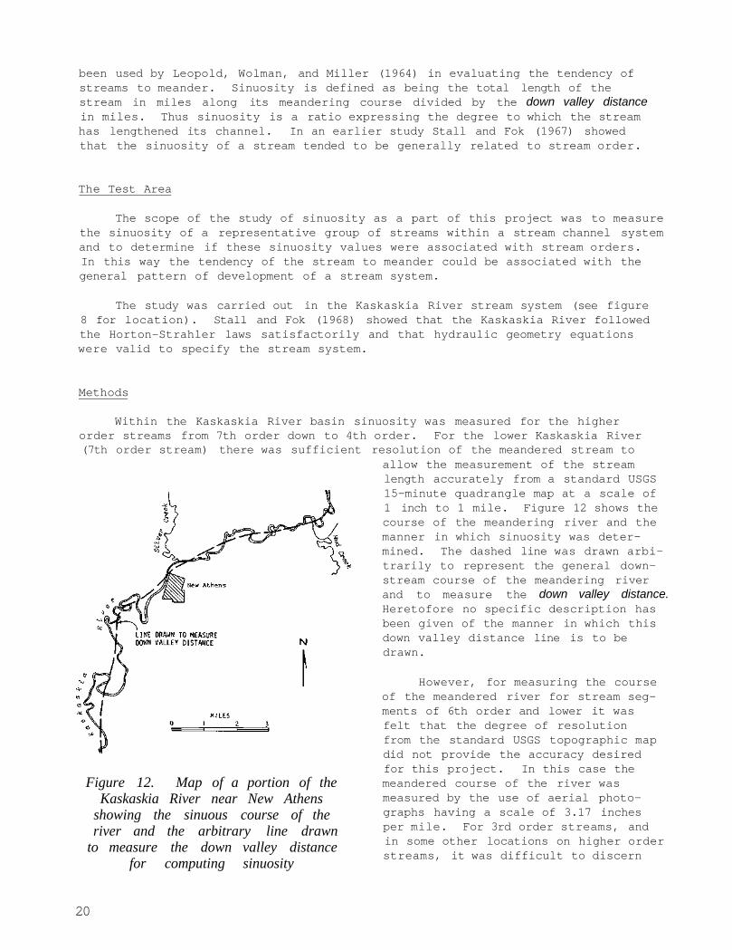
Within the Kaskaskia River basin sinuosity was measured for the higher order streams from 7th order down to 4th order. For the lower Kaskaskia River (7th order stream) there was sufficient resolution of the meandered stream to

Figure 12. Map of a portion of the Kaskaskia River near New Athens

showing the sinuous course of the river and the arbitrary line drawn

to measure the down valley distance for computing sinuosity

allow the measurement of the stream length accurately from a standard USGS 15-minute quadrangle map at a scale of 1 inch to 1 mile. Figure 12 shows the course of the meandering river and the manner in which sinuosity was deter­mined. The dashed line was drawn arbi­trarily to represent the general down­stream course of the meandering river and to measure the down valley distance. Heretofore no specific description has been given of the manner in which this down valley distance line is to be drawn.

However, for measuring the course of the meandered river for stream seg­ments of 6th order and lower it was felt that the degree of resolution from the standard USGS topographic map did not provide the accuracy desired for this project. In this case the meandered course of the river was measured by the use of aerial photo­graphs having a scale of 3.17 inches per mile. For 3rd order streams, and in some other locations on higher order streams, it was difficult to discern

20

the course of the stream because it was obscured by trees and forest. Generally, however, the use of the aerial photographs was successful.

Results

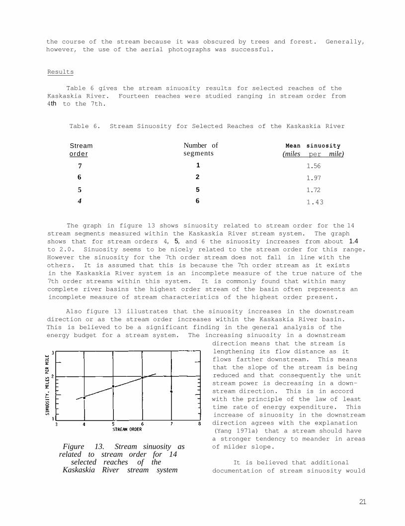
Table 6 gives the stream sinuosity results for selected reaches of the Kaskaskia River. Fourteen reaches were studied ranging in stream order from 4th to the 7th.

Table 6. Stream Sinuosity for Selected Reaches of the Kaskaskia River

The graph in figure 13 shows sinuosity related to stream order for the 14 stream segments measured within the Kaskaskia River stream system. The graph shows that for stream orders 4, 5, and 6 the sinuosity increases from about 1.4 to 2.0. Sinuosity seems to be nicely related to the stream order for this range. However the sinuosity for the 7th order stream does not fall in line with the others. It is assumed that this is because the 7th order stream as it exists in the Kaskaskia River system is an incomplete measure of the true nature of the 7th order streams within this system. It is commonly found that within many complete river basins the highest order stream of the basin often represents an incomplete measure of stream characteristics of the highest order present.

Also figure 13 illustrates that the sinuosity increases in the downstream direction or as the stream order increases within the Kaskaskia River basin. This is believed to be a significant finding in the general analysis of the energy budget for a stream system. The increasing sinuosity in a downstream

direction means that the stream is lengthening its flow distance as it flows farther downstream. This means that the slope of the stream is being reduced and that consequently the unit stream power is decreasing in a down­stream direction. This is in accord with the principle of the law of least time rate of energy expenditure. This increase of sinuosity in the downstream direction agrees with the explanation (Yang 1971a) that a stream should have a stronger tendency to meander in areas of milder slope.

It is believed that additional documentation of stream sinuosity would

Figure 13. Stream sinuosity as related to stream order for 14

selected reaches of the Kaskaskia River stream system

21

Stream order

7 6

5 4

Number of segments

1

2

5 6

Mean sinuosity (miles per mile)

1.56 1.97 1.72 1.43

be desirable in order to further document the tendency of sinuosity to be related to stream order. If this relation is found to be stable within many stream systems, perhaps it can then be generalized as a function of stream order and be predictable to some extent. Such a predictability would aid in the further analysis and understanding of the total energy budget of stream systems.

HYDRAULIC GEOMETRY—UNIT STREAM POWER EQUATIONS

Because of the proven consistency of hydraulic geometry relations within stream systems and because of the seeming consistency of the law of least time rate of energy expenditure of a river system, it seemed feasible to combine these two concepts into a new set of hydraulic geometry—unit stream power equations, which would represent the actual variation of unit stream power throughout a stream system.

A previous study by Stall and Yang (1970) provided hydraulic geometry equa­tions for 12 river basins in the United States. The general relationship between the average velocity and drainage area was shown to be

where V is the average velocity in feet per second, F is the flow frequency, Ad is the drainage area in square miles, and h, i, j are constants.

According to Horton (1945) the law of stream slopes is given as follows

where S is the average slope of the uth order stream in feet per mile, U is the stream order, and a and b are constants.

It was shown by Stall and Fok (1968) that the relation between stream order U and its drainage area Ad can be represented by

where p and g are constants.

By combining equations 12, 13, and 14 we have the expression

where VS is the uni t stream power in foot-pounds per pound per second, which is defined as the time rate of potent ia l energy expenditure per uni t weight of water fo r a natural stream.

22

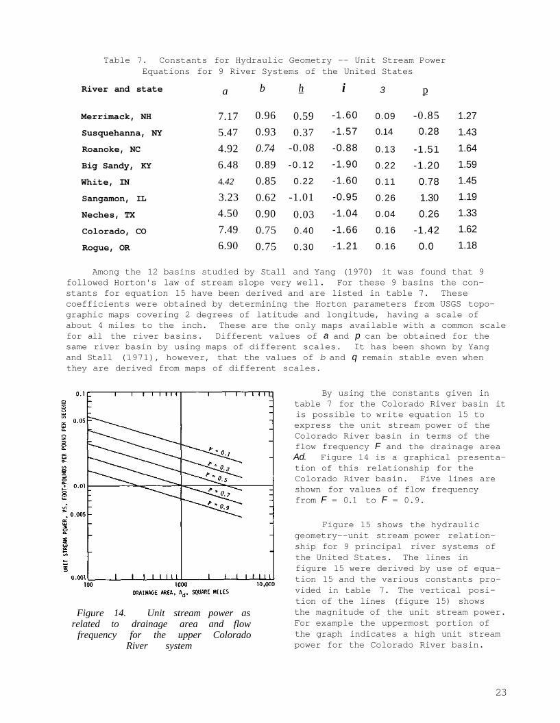
Table 7. Constants for Hydraulic Geometry -- Unit Stream Power Equations for 9 River Systems of the United States

Among the 12 basins studied by Stall and Yang (1970) it was found that 9 followed Horton's law of stream slope very well. For these 9 basins the con­stants for equation 15 have been derived and are listed in table 7. These coefficients were obtained by determining the Horton parameters from USGS topo­graphic maps covering 2 degrees of latitude and longitude, having a scale of about 4 miles to the inch. These are the only maps available with a common scale for all the river basins. Different values of a and p can be obtained for the same river basin by using maps of different scales. It has been shown by Yang and Stall (1971), however, that the values of b and q remain stable even when they are derived from maps of different scales.

Figure 14. Unit stream power as related to drainage area and flow

frequency for the upper Colorado River system

By using the constants given in table 7 for the Colorado River basin it is possible to write equation 15 to express the unit stream power of the Colorado River basin in terms of the flow frequency F and the drainage area Ad. Figure 14 is a graphical presenta­tion of this relationship for the Colorado River basin. Five lines are shown for values of flow frequency from F = 0.1 to F = 0.9.

Figure 15 shows the hydraulic geometry--unit stream power relation­ship for 9 principal river systems of the United States. The lines in figure 15 were derived by use of equa­tion 15 and the various constants pro­vided in table 7. The vertical posi­tion of the lines (figure 15) shows the magnitude of the unit stream power. For example the uppermost portion of the graph indicates a high unit stream power for the Colorado River basin.

23

River and state

Merrimack, NH Susquehanna, NY Roanoke, NC Big Sandy, KY White, IN Sangamon, IL Neches, TX Colorado, CO Rogue, OR

a

7.17 5.47 4.92 6.48 4.42

3.23 4.50 7.49 6.90

b

0.96 0.93 0.74 0.89 0.85 0.62 0.90 0.75 0.75

h

0.59 0.37

-0.08 -0 .12

0.22

-1.01 0.03 0.40

0.30

i

-1.60 -1.57 -0.88 -1.90 -1.60 -0.95 -1.04 -1.66 -1.21

3

0.09

0.14

0.13

0.22

0.11

0.26

0.04

0.16

0.16

p

-0.85 0.28

-1.51 -1.20 0.78 1.30 0.26

-1.42 0.0

1.27 1.43 1.64 1.59 1.45 1.19 1.33 1.62 1.18

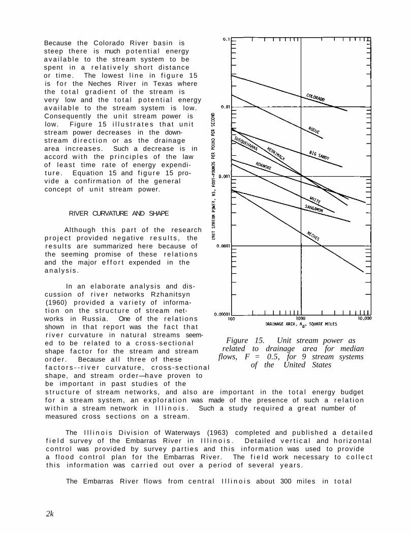
Because the Colorado River bas in is steep there is much p o t e n t i a l energy a v a i l a b l e to the stream system to be spent in a r e l a t i v e l y shor t d i s tance or t ime . The lowest l i n e in f i g u r e 15 is f o r the Neches River in Texas where the t o t a l g rad ien t o f the stream is very low and the t o t a l p o t e n t i a l energy a v a i l a b l e to the stream system is low. Consequently the u n i t stream power is low. F igure 15 i l l u s t r a t e s t h a t u n i t stream power decreases in the down­stream d i r e c t i o n or as the drainage area increases. Such a decrease is in accord w i t h the p r i n c i p l e s of the law of l eas t t ime ra te of energy expendi­t u r e . Equation 15 and f i g u r e 15 pro­vide a con f i rma t i on of the general concept of u n i t stream power.

RIVER CURVATURE AND SHAPE

Although t h i s pa r t o f the research p r o j e c t prov ided negat ive r e s u l t s , the r e s u l t s are summarized here because of the seeming promise of these r e l a t i o n s and the major e f f o r t expended in the a n a l y s i s .

In an e labora te ana lys i s and dis­cussion o f r i v e r networks Rzhanitsyn (1960) prov ided a v a r i e t y of informa­t i o n on the s t r u c t u r e of stream net­works in Russia. One of the r e l a t i o n s shown in t ha t repor t was the f a c t t ha t r i v e r curva ture in na tu ra l streams seem­ed to be re la ted to a c r o s s - s e c t i o n a l shape f a c t o r f o r the stream and stream o rde r . Because a l l th ree of these f a c t o r s - - r i v e r c u r v a t u r e , c r o s s - s e c t i o n a l shape, and stream o rde r—have proven to be important in past s tud ies of the s t r u c t u r e of stream networks , and a lso are important in the t o t a l energy budget f o r a stream system, an e x p l o r a t i o n was made of the presence of such a r e l a t i o n w i t h i n a stream network in I l l i n o i s . Such a study requ i red a great number of measured cross sect ions on a stream.

Figure 15. Unit stream power as related to drainage area for median

flows, F = 0.5, for 9 stream systems of the United States

The I l l i n o i s D i v i s i on of Waterways (1963) completed and pub l i shed a d e t a i l e d f i e l d survey o f the Embarras River in I l l i n o i s . De ta i led v e r t i c a l and h o r i z o n t a l con t ro l was provided by survey p a r t i e s and t h i s i n fo rmat ion was used to prov ide a f l o o d con t ro l p lan f o r the Embarras R iver . The f i e l d work necessary to c o l l e c t t h i s in fo rmat ion was c a r r i e d out over a per iod of several yea rs .

The Embarras River f lows from c e n t r a l I l l i n o i s about 300 mi les in t o t a l

2k

length southward and empties into the Wabash River (see figure 8). Along this reach data were assembled for 853 cross sections from the gaging station at St. Marie, near Newton, to the upstream end of the Embarras River. For the channel section of these cross sections the elevations and shapes were reduced to XY coordinates by the use of the Illinois State Water Survey automatic graphic digitizing machine, the auto-trol, in order to provide complete information on the shape of every cross section.

Also required was a reasonable water surface profile throughout the entire length of the Embarras River in order to specify a flow condition during which the water level of each cross section could be compared with that in all the other cross sections. To provide this water surface profile a computer program was used as published by Eichert (1966). This program was altered to provide for the computation of flows for only the within-the-bank condition. A field inspection trip was made to estimate the Manning roughness coefficients which would seem suitable for use along the river bed.

A water surface profile was computed from the St. Marie gage for the 242 miles upstream to the end of the Embarras River. This profile represented a median flow condition with a frequency of F = 0.50 for all reaches of the river. Water level data for each cross section were used to compute a shape factor, which is the maximum depth at any point in the cross section divided by the stream width.

Extensive plots were made associating this shape factor with the river curvature (the radius of the river bend) and stream order. The results of this entire analysis were widely spread and showed no semblance of structure.

DISPERSION IN STREAMS

When a contaminant or dye is introduced into a stream, it is immediately subject to the natural process of dispersion caused by the differential flow velocities which occur throughout a cross section. The rate of this dispersion is a function of the hydraulic conditions in the stream which to some extent are predictable. This dispersion phenomenon was made a part of the research per­formed in this study because of its importance in water resources planning and its dependence upon hydraulic factors in a stream.

Fischer (1968) provided an authoritative evaluation of the occurrence of dispersion within a stream. Results of his studies were confirmed by dye studies in a hydraulic laboratory and in the Missouri River near Sioux City, Iowa. Addi­tional information on the applicability of this procedure was given by Sooky (1969) who related a river's ability to disperse a contaminant to its channel geometry.

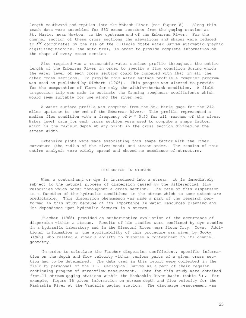
In order to calculate the Fischer dispersion coefficient, specific informa­tion on the depth and flow velocity within various parts of a given cross sec­tion had to be determined. The data used in this report were collected in the field by personnel of the U.S. Geological Survey as a part of their regular continuing program of streamflow measurement. Data for this study were obtained from 11 stream gaging stations within the Kaskaskia River basin (table 8). For example, figure 16 gives information on stream depth and flow velocity for the Kaskaskia River at the Vandalia gaging station. The discharge measurement was

25

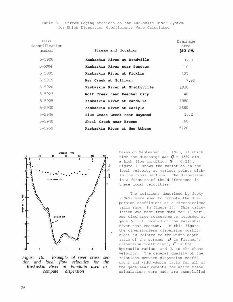
Table 8. Stream Gaging Stations on the Kaskaskia River System for Which Dispersion Coefficients Were Calculated

Figure 16. Example of river cross sec­tion and local flow velocities for the

Kaskaskia River at Vandalia used to compute dispersion

taken on September 16, 1965, at which time the discharge was Q = 1850 cfs, a high flow condition (F = 0.21). Figure 16 shows the variation in the local velocity at various points with­in the cross section. The dispersion is a function of the differences in these local velocities.

The relations described by Sooky (1969) were used to compute the dis­persion coefficient as a dimensionless ratio shown in figure 17. This calcu­lation was made from data for 10 vari­ous discharge measurements recorded at gage 5-5904 located on the Kaskaskia River near Pesotum. In this figure the dimensionless dispersion coeffi­cient is related to the width-depth ratio of the stream. D is Fischer's dispersion coefficient, E is the hydraulic radius, and U* is the shear velocity. The general quality of the relations between dispersion coeffi­cient and width-depth ratio for all of the gage measurements for which these calculations were made are exemplified

26

USGS identification

number

5-5900 5-5904 5-5905 5-5915 5-5920 5-5923 5-5925 5-5930 5-5936 5-5940 5-5950

Stream and location

Kaskaskia River at Bondville Kaskaskia River near Pesotum Kaskaskia River at Ficklin Asa Creek at Sullivan Kaskaskia River at Shelbyville Wolf Creek near Beecher City Kaskaskia River at Vandalia Kaskaskia River at Carlyle Blue Grass Creek near Raymond Shoal Creek near Breese Kaskaskia River at New Athens

Drainage area

(sq mi)

12.3 110 127 7.93

1030 48

1980 2680 17.2

760 5220

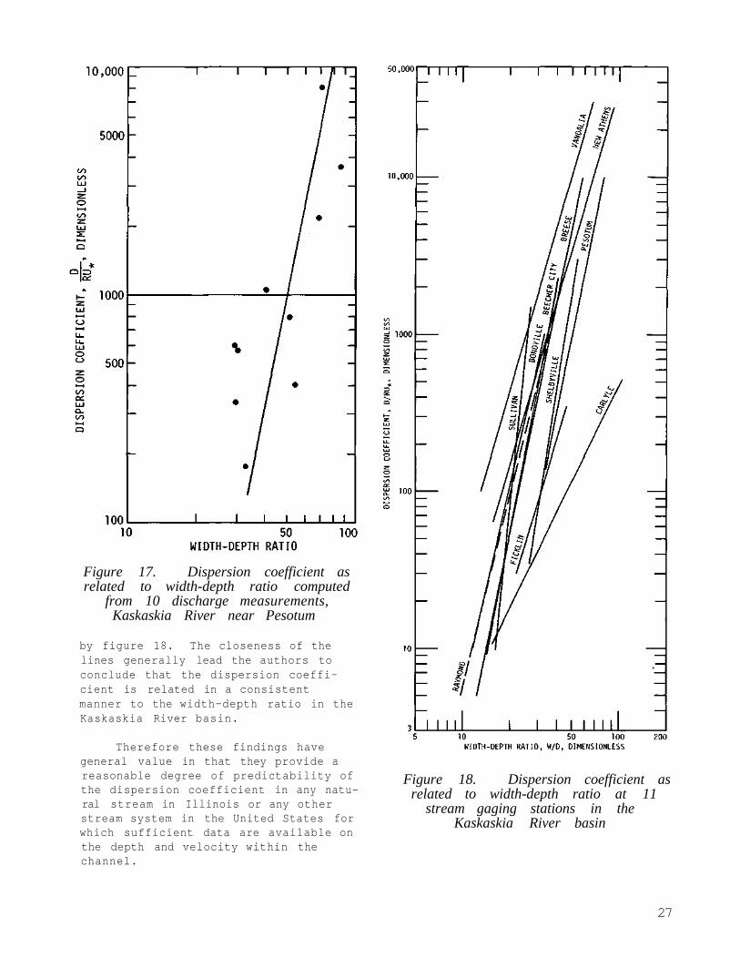
Figure 17. Dispersion coefficient as related to width-depth ratio computed

from 10 discharge measurements, Kaskaskia River near Pesotum

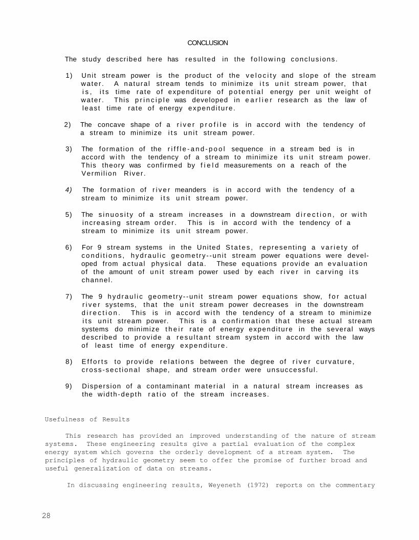
by figure 18. The closeness of the lines generally lead the authors to conclude that the dispersion coeffi­cient is related in a consistent manner to the width-depth ratio in the Kaskaskia River basin.

Therefore these findings have general value in that they provide a reasonable degree of predictability of the dispersion coefficient in any natu­ral stream in Illinois or any other stream system in the United States for which sufficient data are available on the depth and velocity within the channel.

Figure 18. Dispersion coefficient as related to width-depth ratio at 11

stream gaging stations in the Kaskaskia River basin

27

CONCLUSION

The study descr ibed here has resu l ted in the f o l l o w i n g conc lus ions .

1) Un i t stream power is the product of the v e l o c i t y and s lope of the stream wa te r . A na tu ra l stream tends to min imize i t s u n i t stream power, t ha t i s , i t s t ime ra te o f expendi ture o f p o t e n t i a l energy per un i t weight o f wa te r . This p r i n c i p l e was developed in e a r l i e r research as the law of l eas t t ime ra te o f energy expend i t u re .

2) The concave shape of a r i v e r p r o f i l e is in accord w i t h the tendency of a stream to minimize i t s u n i t stream power.

3) The fo rmat ion of the r i f f l e - a n d - p o o l sequence in a stream bed is in accord w i t h the tendency of a stream to minimize i t s u n i t stream power. This theory was conf i rmed by f i e l d measurements on a reach of the Vermi l i on R iver .

4) The fo rmat ion of r i v e r meanders is in accord w i t h the tendency of a stream to minimize i t s u n i t stream power.

5) The s i n u o s i t y of a stream increases in a downstream d i r e c t i o n , or w i t h inc reas ing stream o rde r . This is in accord w i t h the tendency of a stream to minimize i t s u n i t stream power.

6) For 9 stream systems in the Uni ted S t a t e s , represen t ing a v a r i e t y of c o n d i t i o n s , h y d r a u l i c geomet ry - -un i t stream power equat ions were devel­oped from ac tua l phys ica l da ta . These equat ions p rov ide an e v a l u a t i o n of the amount of u n i t stream power used by each r i v e r in ca rv ing i t s channel .

7) The 9 h y d r a u l i c geomet ry - -un i t st ream power equat ions show, f o r ac tua l r i v e r systems, tha t the u n i t stream power decreases in the downstream d i r e c t i o n . This is in accord w i t h the tendency of a stream to minimize i t s u n i t stream power. This is a c o n f i r m a t i o n t ha t these ac tua l stream systems do minimize t h e i r ra te of energy expend i tu re in the severa l ways descr ibed to p rov ide a r e s u l t a n t stream system in accord w i t h the law of leas t t ime of energy e x p e n d i t u r e .

8 ) E f f o r t s to prov ide r e l a t i o n s between the degree o f r i v e r cu rva tu re , c r o s s - s e c t i o n a l shape, and stream order were unsuccess fu l .

9) D ispers ion of a contaminant ma te r i a l in a na tu ra l stream increases as the w id th -dep th r a t i o o f the stream inc reases .

Usefulness of Results

This research has provided an improved understanding of the nature of stream systems. These engineering results give a partial evaluation of the complex energy system which governs the orderly development of a stream system. The principles of hydraulic geometry seem to offer the promise of further broad and useful generalization of data on streams.

In discussing engineering results, Weyeneth (1972) reports on the commentary

28

of Fazlur R. Khan upon being named Construction's Man of the Year:

"I have come to realize that the higher purpose of engineering must be based on the satisfaction of contributing to the overall needs of the entire society by providing choices and solutions that can create better environments for living and working."

The research on hydraulic geometry and the low flow regimen as described in this report has a general usefulness in understanding and predicting the behavior of streams. Theoretical support is provided for the concept that stream behavior is governed by the structure of the potential energy budget of the stream system. Extensive observations on actual natural streams seem to confirm the practical field truth of these theoretical principles.

As Khan has called for, these engineering research results are presented as being useful and creative in the sense that better understanding of stream systems may allow better choices and solutions that can ultimately lead to a better environment for man's living and working.

29

REFERENCES

Chow, Ven Te. 1959. Open-channel hydraulics. McGraw-Hill Book Company, Inc., New York.

Eichert, Bill S. 1966. Backwater at any cross-section. U.S. Army Corps of Engineers, Hydrologic Engineering Center, Generalized Computer Program 22-J2-L212, Davis, California, October.

Fenwick, G. B. 1969. State of knowledge of channel stabilization in major alluvial channels. Corps of Engineers, U.S. Army Committee on Channel Stabilization, Technical Report 7, Vicksburg, Mississippi.

Fischer, Hugo B. 1968. Dispersion predictions in natural streams. American Society of Civil Engineers Sanitary Engineering Division Journal v. 94(SA5): 927-943.

Graf, Walter H. 1971. Hydraulics of sediment transport. McGraw-Hill Book Company, New York.

Horton, Robert E. 1945. Erosional development of streams and their drainage basins—hydrophysical approach to quantitative morphology. Geological Society of America Bulletin v. 56(3):275-370.

Illinois Division of Waterways. 1963. Interim report for flood control and drainage development, Embarras River. Appendix E-Maps, Springfield, 169 pp.

Leopold, Luna B., and Walter B. Langbein. 1962. The concept of entropy in landscape evolution. U.S. Geological Survey Professional Paper 500A.

Leopold, Luna B., and Thomas Maddock. 1953. The hydraulic geometry of stream channels and some physiographic implications. U.S. Geological Survey Professional Paper 252.

Leopold, Luna B., M. Gordon Wolman, and John P. Miller. 1964. Fluvial processes in geomorphology. W. H. Freeman and Co., San Francisco, p. 281.

Morisawa, Marie. 1968. Streams, their dynamics and morphology. McGraw-Hill Book Co., New York.

Posey, C. J. 1950. Chapter IX. Gradually varied channel flow. In Engineering Hydraulics, edited by Hunter Rouse, John Wiley and Sons, p. 617-621.

Rzhanitsyn, N. A. 1960. Morphological and hydrological regularities of the structures of the river net. Translated from Russian by D. B. Krimgold, Agricultural Research Service, USDA.

Scheidegger, A. E. 1964. Some implications of statistical mechanics in geomorphology. International Association of Scientific Hydrology Bulletin v. 9(0 : 12-16.

30

Schumm, S. A. 1963. Tentative classification of al luvial river channels. U.S. Geological Survey Circular 477, Washington, D.C.

Simons, D. B., and E. V. Richardson. 1966. Resistance to flow in alluvial channels. U.S. Geological Survey Professional Paper 442-J.

Sooky, Attila A. 1969. Longitudinal dispersion in open channels. American Society of Civil Engineers, Journal of the Hydraulics Division v. 95(HY4): 1327, July.

Stall, John B., and Douglas W. Hiestand. 1969. Provisional time-of-travel for Illinois streams. Illinois State Water Survey Report of Investigation 63.

Stall, John B., and Yu-Si Fok. 1967. Discharge as related to stream system morphology. International Association of Scientific Hydrology Symposium on River Morphology, Publication 75, Gentbrugge, Belgium, p. 224-235.

Stall, John B., and Yu-Si Fok. 1968. Hydraulic geometry of Illinois streams. University of Illinois Water Resources Center, Urbana, Research Report 15.

Stall, John B., and C. T. Yang. 1970. Hydraulic geometry of 12 selected stream systems of the United States. University of Illinois Water Resources Center Research Report No. 32, Urbana.

Weyeneth, Eugene E. 1972. To fill you in. Engineering News-Record v. 188(7): 5.

Yang, C. T. 1971a. Potential energy and stream morphology. Water Resources Research v. 7(2): 311-322.

Yang, C. T. 1971b. On river meanders. Journal of Hydrology v. 13(3): 231-253.

Yang, C. T. 1971c. Formation of riffles and pools. Water Resources Research v. 7(6): 1567-1574.

Yang, C. T. 1972. Unit stream power and sediment transport. ASCE Hydraulics Division Conference, Cornell University, Ithaca, N.Y.

Yang, C. T., and John B. Stall. 1971. Note on the map scale effect in the study of stream morphology. Water Resources Research v. 7(3): 709-712.

31