Image-Guided Targeting and Control of Implantable Electrodes

By

Louis Beryl Kratchman

Dissertation

Submitted to the Faculty of the

Graduate School of Vanderbilt University

partial fulfillment of the requirements

for the degree of

DOCTOR OF PHILOSOPHY

in

Mechanical Engineering

May, 2015

Nashville, Tennessee

Approved:

Robert J. Webster, III

Nabil Simaan

Pietro Valdastri

J. Michael Fitzpatrick

Robert F. Labadie

To my wife Clare, Max, and Zack

ii

ACKNOWLEDGMENTS

I thank my adviser, Bob Webster, for his encouragement over the years, his openness

to new ideas, and for widening my perspective about our work. He has challenged me to make

the maximum impact, in research and beyond.

I am indebted to Robert Labadie and Michael Fitzpatrick for welcoming me into the

CAOS Lab, guiding my research, serving on my thesis committee, and for their enthusiasm

and humor. The creativity and teamwork I’ve experienced in the CAOS Lab has left a deep

impression on me. I could not have completed the work in this thesis without the contributions

from past and present CAOS Lab members Ramya Balachandran, Grégoire Blachon, Maria

Ashby, Lueder Kahrs, Wendy Lipscomb, and Kate Von Wahlde. Thank you all for sharing

your talents and energy.

Outside of the lab, I’ve relied on the steadfast support of my wife, and the love and

counsel of my parents.

My sincere thanks to committee members Nabil Simaan and Pietro Valdastri for their

time, comments, and attention to this manuscript.

To all the graduate students, postdocs, and undergraduates in the MED Lab whom I

have worked with, thank you for making my time at Vanderbilt pleasurable. I would especially

like to thank undergraduates Mish Rahman, Justin Saunders, and Yifan Zhu for their help and

commitment to various projects.

I would also like to thank Brent Gillespie and Johann Borenstein at the University of

Michigan, who helped interest me in research.

iii

I owe thanks to several others who made special contributions to this dissertation.

Tom Withrow was instrumental in bringing Chapter 2 to fruition. John Fitzpatrick at FHC

Corporation graciously provided the data discussed in the Appendix to Chapter 3. My chapter

4 co-author Daniel Schuster was a great partner in experiments. Neil Dillon helped us set

up experimental equipment for Chapter 5, and Hunter Gilbert and Richard Hendrick shared

valuable insights on the theory of elastic rods.

iv

ABSTRACT

Implantable electrodes are used to diagnose and treat a growing list of conditions,

including deafness, chronic pain, and neurodegenerative disorders. This dissertation introduces

robotic methods to make electrode implantation less invasive, safer, and easier for clinicians

to perform. We focus on implantation through a narrow hole under image guidance, and

contribute methods to both guide instruments along a straight insertion path and to steer

electrodes that are inserted through such a hole.

We present the first bone-attached robot to accurately guide instruments to the cochlea.

This system removes the need to fabricate a stereotactic guide in the operating room and reduces

dependence on a surgeon’s skill. Results from a phantom targeting experiment show this system

to be suciently accurate for cochlear implantation surgery. Manually adjusted stereotactic

frames are used to implant deep brain stimulation (DBS) electrodes, but encumber the patient and

are prone to operator errors. Smaller targeting devices are available for DBS surgery, but require

osite manufacturing or expensive image guidance systems. We introduce robotically adjusted,

disposable microstereotactic frames that are rapidly adjusted, locked, and then transferred to a

patient in a single visit. A phantom validation experiment shows that the targeting error of a

robotically adjusted frame was below the clinically accepted threshold.

Sensitive tissues can be damaged by the force of electrode implantation. Robotic

insertion devices have the potential to detect and react to excessive insertion forces, but the

relationship between forces and trauma is poorly understood. Presently, we rely on surgeons

to judge when forces are too large, but the ability of surgeons to sense small forces when

v

implanting electrodes has not been studied. We introduce a method to measure intraocochlear

puncture forces and report the first force measurements obtained from fresh cadaveric specimens.

To put these forces into a clinical perspective, we present a protocol to measure tactile thresholds

in a model of CI surgery, and present the first experimental characterization of surgeons’ tactile

force thresholds.

An electrode can be actively steered to reduce trauma and avoid obstacles. We present

the first method to guide a magnet-tipped electrode along arbitrary three-dimensional trajecto-

ries using a compact, robot-manipulated magnet located external to the patient. We model rod

deflections by combining Kirchho rod theory with permanent magnet models, and compute

trajectories using a resolved-rate approach. Experiments demonstrate accurate execution of

three-dimensional tip trajectories in an open-loop configuration and obstacle avoidance.

This dissertation provides a complementary set of methods for improving electrode

implantation. These methods could benefit both patients and clinicians who perform minimally

invasive procedures.

vi

CONTENTS

Dedication ii

Acknowledgments iii

Abstract v

List of Tables xi

1 Introduction 11.1 Stereotactic Frames . . . . . . . . . . . . . . . . . . . . . . . . . . . . . . . . . . . . . . 1

1.1.1 Frameless Stereotactic Systems . . . . . . . . . . . . . . . . . . . . . . . . . . . 41.1.2 Robotic Stereotactic Surgery . . . . . . . . . . . . . . . . . . . . . . . . . . . . 61.1.3 Custom-manufactured stereotactic frames . . . . . . . . . . . . . . . . . . . . . 71.1.4 Contributions . . . . . . . . . . . . . . . . . . . . . . . . . . . . . . . . . . . . 9

2 Design of a Bone-Attached Parallel Robot for Percutaneous Cochlear Implantation 112.1 Introduction . . . . . . . . . . . . . . . . . . . . . . . . . . . . . . . . . . . . . . . . . 112.2 Surgical workflow . . . . . . . . . . . . . . . . . . . . . . . . . . . . . . . . . . . . . . 152.3 AIM Frame Robot Design . . . . . . . . . . . . . . . . . . . . . . . . . . . . . . . . . . 17

2.3.1 Clinical Dataset Processing: Obtaining Drill Trajectories . . . . . . . . . . . . 172.3.2 The Pre-Positioning Frame . . . . . . . . . . . . . . . . . . . . . . . . . . . . . 182.3.3 Actuators and Encoders . . . . . . . . . . . . . . . . . . . . . . . . . . . . . . . 192.3.4 Robot Structure . . . . . . . . . . . . . . . . . . . . . . . . . . . . . . . . . . . 212.3.5 Control System . . . . . . . . . . . . . . . . . . . . . . . . . . . . . . . . . . . 232.3.6 Attachment of surgical tools . . . . . . . . . . . . . . . . . . . . . . . . . . . . 23

2.4 Experimental Results . . . . . . . . . . . . . . . . . . . . . . . . . . . . . . . . . . . . . 242.4.1 Free-Space Targeting Experiment . . . . . . . . . . . . . . . . . . . . . . . . . 242.4.2 Cadaver Drilling Experiment . . . . . . . . . . . . . . . . . . . . . . . . . . . . 26

2.5 Conclusion and Future Work . . . . . . . . . . . . . . . . . . . . . . . . . . . . . . . . 28

3 Robotically-Adjustable Microstereotactic Frames for Image-Guided Neurosurgery 313.1 Introduction . . . . . . . . . . . . . . . . . . . . . . . . . . . . . . . . . . . . . . . . . 313.2 Microstereotactic Frame Design . . . . . . . . . . . . . . . . . . . . . . . . . . . . . . 343.3 Microstereotactic Frame Adjustment and Locking . . . . . . . . . . . . . . . . . . . . 393.4 Proposed Clinical Workflow . . . . . . . . . . . . . . . . . . . . . . . . . . . . . . . . 423.5 Methods . . . . . . . . . . . . . . . . . . . . . . . . . . . . . . . . . . . . . . . . . . . . 433.6 Results . . . . . . . . . . . . . . . . . . . . . . . . . . . . . . . . . . . . . . . . . . . . . 483.7 Conclusions . . . . . . . . . . . . . . . . . . . . . . . . . . . . . . . . . . . . . . . . . . 49

4 Measurement and Perception of Traumatic Forces in Cochlear Implantation Surgery 504.1 Introduction . . . . . . . . . . . . . . . . . . . . . . . . . . . . . . . . . . . . . . . . . 514.2 Materials and Methods . . . . . . . . . . . . . . . . . . . . . . . . . . . . . . . . . . . . 534.3 Results . . . . . . . . . . . . . . . . . . . . . . . . . . . . . . . . . . . . . . . . . . . . . 58

vii

4.4 Discussion . . . . . . . . . . . . . . . . . . . . . . . . . . . . . . . . . . . . . . . . . . . 604.5 Measurement of surgeon force perception thresholds in cochlear implantation . . . . . 62

4.5.1 Methods . . . . . . . . . . . . . . . . . . . . . . . . . . . . . . . . . . . . . . . 654.5.2 Results . . . . . . . . . . . . . . . . . . . . . . . . . . . . . . . . . . . . . . . . 714.5.3 Discussion . . . . . . . . . . . . . . . . . . . . . . . . . . . . . . . . . . . . . . 72

4.6 Conclusion . . . . . . . . . . . . . . . . . . . . . . . . . . . . . . . . . . . . . . . . . . 73

5 Guiding Elastic Rods with a Permanent Magnet for Medical Applications 745.1 Introduction . . . . . . . . . . . . . . . . . . . . . . . . . . . . . . . . . . . . . . . . . 745.2 Application : magnet-guided cochlear implantation surgery . . . . . . . . . . . . . . . 775.3 Permanent-Magnet Models . . . . . . . . . . . . . . . . . . . . . . . . . . . . . . . . . 81

5.3.1 Force and Torque on Tip Magnet . . . . . . . . . . . . . . . . . . . . . . . . . 815.3.2 External Magnet Field Models . . . . . . . . . . . . . . . . . . . . . . . . . . . 82

5.4 Magnet-Tipped Rod Model . . . . . . . . . . . . . . . . . . . . . . . . . . . . . . . . . 845.4.1 Kinematics . . . . . . . . . . . . . . . . . . . . . . . . . . . . . . . . . . . . . . 845.4.2 Constitutive Relations . . . . . . . . . . . . . . . . . . . . . . . . . . . . . . . . 855.4.3 Equilibrium Equations . . . . . . . . . . . . . . . . . . . . . . . . . . . . . . . . 875.4.4 Boundary Conditions . . . . . . . . . . . . . . . . . . . . . . . . . . . . . . . . 885.4.5 Numerical Solutions . . . . . . . . . . . . . . . . . . . . . . . . . . . . . . . . . 92

5.5 Trajectory Following . . . . . . . . . . . . . . . . . . . . . . . . . . . . . . . . . . . . 945.5.1 Forward Kinematics . . . . . . . . . . . . . . . . . . . . . . . . . . . . . . . . . 945.5.2 Inversion and Redundancy Resolution . . . . . . . . . . . . . . . . . . . . . . . 955.5.3 Avoiding an Obstacle Using a Virtual Wall . . . . . . . . . . . . . . . . . . . . 96

5.6 Experimental Methods . . . . . . . . . . . . . . . . . . . . . . . . . . . . . . . . . . . . 995.6.1 Advancer and Magnet-Tipped Rod . . . . . . . . . . . . . . . . . . . . . . . . 995.6.2 Robot and External Magnet . . . . . . . . . . . . . . . . . . . . . . . . . . . . . 1005.6.3 Trajectory Computation and Control . . . . . . . . . . . . . . . . . . . . . . . 1025.6.4 Stereo Camera Measurements . . . . . . . . . . . . . . . . . . . . . . . . . . . 1035.6.5 Calibration . . . . . . . . . . . . . . . . . . . . . . . . . . . . . . . . . . . . . . 103

5.7 Experiments . . . . . . . . . . . . . . . . . . . . . . . . . . . . . . . . . . . . . . . . . 1055.8 Conclusion . . . . . . . . . . . . . . . . . . . . . . . . . . . . . . . . . . . . . . . . . . 109

6 Conclusions 1116.1 Improvements to Stereotactic Surgery Using Robots . . . . . . . . . . . . . . . . . . . 1116.2 Force thresholds in CI surgery . . . . . . . . . . . . . . . . . . . . . . . . . . . . . . . 1146.3 Guiding magnet-tipped electrodes . . . . . . . . . . . . . . . . . . . . . . . . . . . . . 1156.4 Outlook . . . . . . . . . . . . . . . . . . . . . . . . . . . . . . . . . . . . . . . . . . . . 116

Bibliography 125

viii

LIST OF FIGURES

1.1 Stereotactic frames . . . . . . . . . . . . . . . . . . . . . . . . . . . . . . . . . . . . . . 21.2 Frameless Systems . . . . . . . . . . . . . . . . . . . . . . . . . . . . . . . . . . . . . . 41.3 Stereotactic robots . . . . . . . . . . . . . . . . . . . . . . . . . . . . . . . . . . . . . . 61.4 Custom-manufactured stereotactic devices . . . . . . . . . . . . . . . . . . . . . . . . . 8

2.1 Cochlear implant system . . . . . . . . . . . . . . . . . . . . . . . . . . . . . . . . . . . 122.2 The Microtable . . . . . . . . . . . . . . . . . . . . . . . . . . . . . . . . . . . . . . . . 142.3 The AIM Frame prototype . . . . . . . . . . . . . . . . . . . . . . . . . . . . . . . . . 162.4 The surgical workflow for PCI using the AIM Frame. . . . . . . . . . . . . . . . . . . 172.5 Segmentation of a patient CT scan . . . . . . . . . . . . . . . . . . . . . . . . . . . . . 182.6 Schematic diagram of AIM Frame with PCI trajectories . . . . . . . . . . . . . . . . . 192.7 The pre-positioning frame . . . . . . . . . . . . . . . . . . . . . . . . . . . . . . . . . . 202.8 Motor-actuated prismatic leg joint . . . . . . . . . . . . . . . . . . . . . . . . . . . . . 212.9 The AIM Frame with attached drill press. . . . . . . . . . . . . . . . . . . . . . . . . . 242.10 Phantom used for free-space targeting trials . . . . . . . . . . . . . . . . . . . . . . . . 252.11 Results from free-space targeting trials . . . . . . . . . . . . . . . . . . . . . . . . . . . 272.12 Post-drilling CT scan of cadaveric temporal bone . . . . . . . . . . . . . . . . . . . . . 28

3.1 Traditional stereotactic frames versus microstereotactic frames . . . . . . . . . . . . . . 333.2 Freeze Frame with electrode drive unit attached . . . . . . . . . . . . . . . . . . . . . . 353.3 Analysis of clinical patient data . . . . . . . . . . . . . . . . . . . . . . . . . . . . . . . 363.4 Degrees of Freedom of Freeze Frame legs . . . . . . . . . . . . . . . . . . . . . . . . . 383.5 Proposed Freeze Frame adjustment process . . . . . . . . . . . . . . . . . . . . . . . . 413.6 CNC milling machine used to adjust the Freeze Frame during experiments . . . . . . 443.7 Measurement of adjusted Freeze Frame . . . . . . . . . . . . . . . . . . . . . . . . . . 46

4.1 Cochlear schematic . . . . . . . . . . . . . . . . . . . . . . . . . . . . . . . . . . . . . . 524.2 Experimental apparatus for intracochlear puncture . . . . . . . . . . . . . . . . . . . . 544.3 Orientation of specimen . . . . . . . . . . . . . . . . . . . . . . . . . . . . . . . . . . . 554.4 Specimen before rupture . . . . . . . . . . . . . . . . . . . . . . . . . . . . . . . . . . . 564.5 Puncture of interscalar partition . . . . . . . . . . . . . . . . . . . . . . . . . . . . . . . 574.6 Magnet-guided cochlear implantation . . . . . . . . . . . . . . . . . . . . . . . . . . . 594.7 Psychometric function . . . . . . . . . . . . . . . . . . . . . . . . . . . . . . . . . . . . 634.8 Tactile threshold testing device . . . . . . . . . . . . . . . . . . . . . . . . . . . . . . . 684.9 Tactile threshold study participant . . . . . . . . . . . . . . . . . . . . . . . . . . . . . 694.10 Two-alternative forced-choice staircase plot . . . . . . . . . . . . . . . . . . . . . . . . 71

5.1 Magnet-guided cochlear implantation . . . . . . . . . . . . . . . . . . . . . . . . . . . 805.2 Arrangement of magnets . . . . . . . . . . . . . . . . . . . . . . . . . . . . . . . . . . 835.3 Kirchho rod model . . . . . . . . . . . . . . . . . . . . . . . . . . . . . . . . . . . . . 855.4 Rod force balance . . . . . . . . . . . . . . . . . . . . . . . . . . . . . . . . . . . . . . 875.5 Rod, with bushing . . . . . . . . . . . . . . . . . . . . . . . . . . . . . . . . . . . . . . 895.6 Rod, without bushing . . . . . . . . . . . . . . . . . . . . . . . . . . . . . . . . . . . . 91

ix

5.7 Experimental apparatus for magnetic steering . . . . . . . . . . . . . . . . . . . . . . . 1005.8 Robot and advancer . . . . . . . . . . . . . . . . . . . . . . . . . . . . . . . . . . . . . 1015.9 Orthogonal square trajectories . . . . . . . . . . . . . . . . . . . . . . . . . . . . . . . 1065.10 Concho-spiral trajectory . . . . . . . . . . . . . . . . . . . . . . . . . . . . . . . . . . . 1075.11 Square trajectory, with virtual wall . . . . . . . . . . . . . . . . . . . . . . . . . . . . . 1085.12 Trefoil knot trajectory with 2-DOF robot . . . . . . . . . . . . . . . . . . . . . . . . . 110

6.1 Miniature Freeze Frame concept . . . . . . . . . . . . . . . . . . . . . . . . . . . . . . 1136.2 STarFix designs in dataset . . . . . . . . . . . . . . . . . . . . . . . . . . . . . . . . . . 1186.3 Least-squares fits to fiducial positions . . . . . . . . . . . . . . . . . . . . . . . . . . . . 1206.4 Permanent magnet field models . . . . . . . . . . . . . . . . . . . . . . . . . . . . . . . 123

x

LIST OF TABLES

2.1 Robot design parameters . . . . . . . . . . . . . . . . . . . . . . . . . . . . . . . . . . . 22

3.1 Freeze Frame experimental results . . . . . . . . . . . . . . . . . . . . . . . . . . . . . 48

4.1 Demographics of participants included in analysis of force perception thresholds. . . . . 664.2 Semmes-Weinstein monofilaments . . . . . . . . . . . . . . . . . . . . . . . . . . . . . 674.3 Force perception threshold statistics from ten otolaryngological surgeons. . . . . . . . 71

5.1 Calibrated values of model parameters . . . . . . . . . . . . . . . . . . . . . . . . . . . 1055.2 Rod tip error . . . . . . . . . . . . . . . . . . . . . . . . . . . . . . . . . . . . . . . . . 105

6.1 Frame anchor dataset . . . . . . . . . . . . . . . . . . . . . . . . . . . . . . . . . . . . 117

xi

CHAPTER 1

INTRODUCTION

Cochlear implants have been described as the most successful neural prostheses [1]. Without

these devices, over 300,000 recipients worldwide would be unable to hear. In the United States, approxi-

mately 1.5 million people are considered eligible for the surgery [2], but have not received the treatment

for a variety of reasons. Can cochlear implants be made more accessible to those suering from severe

hearing loss? Can the success of cochlear implants be replicated or surpassed by emerging treatments

that also use implantable electrodes, such as deep brain stimulation and other neuromodulation therapies?

The answers to these questions will depend in part on the tools and techniques available for electrode

implantation. This thesis proposes methods to improve the safety, invasiveness, and clinical practicability

of electrode implantation. For background to the next two chapters, which introduce new stereotactic

devices for electrode implantation, the remainder of this chapter reviews stereotactic targeting devices

which preceded our work.

1.1 Stereotactic Frames

Stereotactic surgery uses an apparatus to guide an instrument to a target within the head or other area of

the body where anatomical structures have a rigid spatial arrangement, such as the spine. The instrument

is guided using a three-dimensional representation of the patient’s anatomy, which may be a surgical

atlas or a medical image. The traditional instrument for stereotactic surgery is the stereotactic frame,

though several other devices are used clinically and will be discussed in this chapter.

The stereotactic frame was introduced by Horsley and Clarke in 1908 [3]. Previous devices

were constructed to identify particular regions of the brain or the cortex with respect to landmarks

1

on the skull, but Horsley and Clarke built the first device able to probe the entire three-dimensional

volume of an animal brain [4], and to relate coordinates to a brain atlas. They built several models, none

of which were used on humans. The first human stereotactic neurosurgery was performed by Ernest

Spiegel and Henry Wycis in 1947, who identified brain landmarks in x-ray images to guide a probe,

sparking worldwide interest in stereotactic surgery and development of new stereotactic frames [5].

(a) (b) (c) (d)

Figure 1.1: Stereotactic frames in current use include the (a) Leksell frame, shown with attached endo-scope1 (b) Zamorano-Dujovny2 frame (c) Cosman-Roberts-Wells frame 3 (d) and Riechert-Mundingerframe4.

Several stereotactic frames in current clinical use are shown in Figure 1.1. Prior to surgery, a

base ring is attached to a patient by tightening four or more sharpened pins into the scalp. The base ring

establishes a coordinate system in rigid relation to patient anatomy. A localizer device that encloses the

patient’s head is attached to the base ring for acquisition of pre-operative images. Localizers are available

for computed tomography (CT), magnetic resonance imaging (MRI), and angiographic imaging. The

localizer contains fiducial markers that enable registration of surgical targets to the stereotactic coordinate

system. Fiducial localization and selection of target and entry points is usually performed with stereotactic

planning software. To perform the surgery, the localizer is replaced by a mechanical apparatus that is1Image: Elekta AB, www.elekta.com, accessed March 3, 2015.2Image: inomed Medizintechnik GmbH, www.inomed.com, accessed March 3, 2015.3Image: Integra LifeSciences, www.integralife.com, accessed March 3, 2015.4Image: inomed Medizintechnik GmbH, www.inomed.com, accessed March 3, 2015.

2

manually adjusted to guide an instrument such as an electrode advancer, endoscope, or cannula to the

target. Coordinate settings are calculated with the aid of the planning software and transferred to several

adjustable components with engraved markings on the frame. Frames such as the Cosman-Roberts-Wells

(CRW) and Riechert-Mundinger (RM) have a separate base that can position a phantom target to check

the accuracy of an adjusted frame before it is used in surgery.

Stereotactic frames are the conventional apparatus for stereotactic neurosurgeries, and are

indicated for a wide range of procedures, including functional neurosurgical procedures, such as electrode

placement for deep brain stimulation surgery or treatment of intractable pain, and non-functional

procedures such as biopsy ablation, cyst drainage, and hematoma evacuation [6, 7]. Clinicians are

experienced at using stereotactic frames, and a large body of published studies documents the clinical

use of these devices [5]. Current frames can reach targets throughout the brain volume and can be

repositioned during surgery. The mechanical designs of these devices have been refined over several

decades, resulting in durable instruments that perform reliably after many surgeries.

However, traditional stereotactic frames have several drawbacks which have motivated develop-

ment of the alternative approaches to be discussed shortly. The heavy, cage-like structure of these devices

causes anxiety in many patients who are required to remain conscious during certain neurosurgical

procedures, and may suer from movement disorders that further increase discomfort. For clinicians,

assembly of a frame from its sterilization tray components is a tedious, time-consuming process, as is the

process of securing the frame to the patient using fixation pins. During surgery, frames may obstruct

access to the patient. Accurate frame adjustment requires repeated transfer of coordinates from planning

software to adjustable scales at several locations on a frame. Flickinger et al. [8] examined 200 clinical

cases of stereotactic frame adjustment for radiosurgery and found coordinate errors in 12 percent of the

cases. The authors found that two additional observers were required to check coordinates in order to

3

reduce the error rate to an acceptable level.

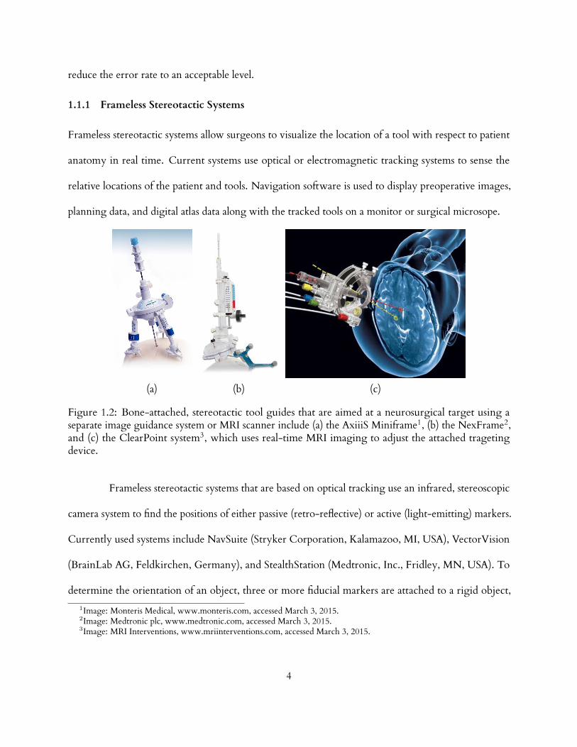
1.1.1 Frameless Stereotactic Systems

Frameless stereotactic systems allow surgeons to visualize the location of a tool with respect to patient

anatomy in real time. Current systems use optical or electromagnetic tracking systems to sense the

relative locations of the patient and tools. Navigation software is used to display preoperative images,

planning data, and digital atlas data along with the tracked tools on a monitor or surgical microsope.

(a) (b) (c)

Figure 1.2: Bone-attached, stereotactic tool guides that are aimed at a neurosurgical target using aseparate image guidance system or MRI scanner include (a) the AxiiiS Miniframe1, (b) the NexFrame2,and (c) the ClearPoint system3, which uses real-time MRI imaging to adjust the attached tragetingdevice.

Frameless stereotactic systems that are based on optical tracking use an infrared, stereoscopic

camera system to find the positions of either passive (retro-reflective) or active (light-emitting) markers.

Currently used systems include NavSuite (Stryker Corporation, Kalamazoo, MI, USA), VectorVision

(BrainLab AG, Feldkirchen, Germany), and StealthStation (Medtronic, Inc., Fridley, MN, USA). To

determine the orientation of an object, three or more fiducial markers are attached to a rigid object,1Image: Monteris Medical, www.monteris.com, accessed March 3, 2015.2Image: Medtronic plc, www.medtronic.com, accessed March 3, 2015.3Image: MRI Interventions, www.mriinterventions.com, accessed March 3, 2015.

4

such as a patient’s head or a rigid tracking frame attached to a tool, and the orientation of the object is

determined from the relative positions of a set of markers. Optical tracking systems require a line of site

to be maintained between the tracker camera and the tracked object.

Electromagnetic tracking systems, such as the Cygnus Stereotactic System (Compass In-

ternational, Inc., Rochester, MN, USA), StealthStation AxiEM (Medtronic Inc.), and InstaTrak (GE

Healthcare), use a field generator project a magnetic field through the operative region. Induced currents

in a small coil embedded in an instrument are measured to determine the instrument’s location. The

coil can be embedded near the tip of the instrument because a line of sight is not required to track the

coil. Metallic objects in the operating suite can distort the field, so precautions are required to maintain

accuracy.

Several types of instrument guides are used for applications where a freehand approach to

guiding a tracked instrument does not provide sucient accuracy or stability. These devices are

positioned using an image guidance system and then locked, and include articulated positioning arms,

burrhole-mounted devices, and bone-attached devices [9]. Bone-attached devices are anchored at

several points around the entry hole, and include The NexFrame system (Medtronic, Inc.), Axiiis

Stereotactic Miniframe (Monteris Medical Corp., Plymouth, MN, USA), and the ClearPoint system

(MRI Interventions, Irvine, CA, USA), which are shown in Figure 1.2. The ClearPoint system processes

MRI images in real-time, and guides a surgeon to adjust control knobs on the frame to align the device

with a planned trajectory.

Frameless systems have been increasingly used for procedures such as brain biopsy and brain

tumor removal [10]. However, these systems rely on expensive image guidance systems and surgeon

hand-eye coordination for accurate adjustment.

5

1.1.2 Robotic Stereotactic Surgery

In 1985 Kwoh et al. used an industrial robot to biopsy a brain tumor, the first published report of a robot

used in human surgery and a precursor to later robotic stereotactic systems [11, 12]. The base ring from

a stereotactic frame was attached to a patient’s scalp, and a CT scan was used to localize the tumor with

respect to a localizer frame attached to the base ring. The system was eventually retired after twelve

successful surgeries [13]. A number robotic systems for stereotactic and general neurosurgical tasks were

constructed following Kwoh et al. [13,14]. Three FDA-approved, commercial systems in current clinical

use are shown in Figure 1.3. These include the Neuromate (Renishaw plc, Wotton-under-Edge, United

Kingdom), Rosa (MedTech S.A.S, Castelnau Le Lez, France), and Renaissance (Mazor Robotics Ltd.,

Caesarea, Israel) systems.

(a) (b) (c)

Figure 1.3: Clinically-approved stereotactic robots include the (a) The NeuroMate1 (b) Rosa2 (c)Renaissance systems3.

As with other stereotactic devices, a stereotactic robot must be registered to pre-operative

images for accurate targeting. A patient’s head may be immobilized by rigid pins and rigidly connected1Image: Renishaw plc, www.renishaw.com, accessed March 3, 2015.2Image: Medtech SAS, www.medtech.fr, accessed March 3, 2015.3Image: Mazor Robotics, www.mazorrobotics.com, accessed March 3, 2015.

6

to the robot base, or an image guidance system may be used in a frameless approach. Both the Neuromate

and Rosa systems can be used with a frameless approach. The miniature parallel robot of the Mazor

Renaissance system [15] is attached directly to bone, which eliminates relative motion between the

robot base and the patient without immobilizing the robot or the patient’s body. The primary surgical

application of the system is pedicle screw placement in the spine, but may also be used in neurosurgery,

and has recently been approved by the Food and Drug Administration (FDA) for deep-brain stimulation

surgery [14].

Robotic stereotactic systems may be advantageous for procedures that require frequent reposi-

tioning of tools, such as neuroendoscopy and stereoelectroencephalography (SEEG). Though robots

are not susceptible to the cognitive errors that human clinicians may be susceptible to when adjusting a

stereotactic device, there is always a risk of mechanical or electrical malfunction with such devices.

1.1.3 Custom-manufactured stereotactic frames

The STarFix microTargeting Platform (FHC Inc., Bowdoin, ME, USA) is an FDA-approved system

for implantation of electrodes for deep brain stimulation, and requires no manual adjustments [16].

Rather, each STarFix is custom-manufactured using patient-specific data to be pre-aimed at a target.

Prior to surgery, three or four titanium anchors are implanted on a patient’s scalp followed by CT and

MR image acquisition. The patient then leaves the surgical site with the anchors in place. Planning

software is used to register the CT scan to the MR scan, localize the anchors in the CT image, and

select a target in the MR image. The planning data is transmitted to a special site where the STarFix

is manufactured using a three-dimensional printing process, and then is delivered to the surgical site

after approximately three days. During surgery, the STarFix is bolted to the pre-implanted anchors, and

supports an electrode driver. The STarFix is a compact, light weight fixture that eliminates the need for

manual frame adjustment, but the time delay required for manufacturing the device is an inconvenience

7

for patients.

MicrotableSTarFix

(a) (b)

Figure 1.4: Custom-manufactured stereotactic devices. (a) The STarFix platform1 is manufactured usingthree dimensional laser sintering technology at a special facility and used for electrode implantationduring deep-brain stimulation surgery. (b) The Microtable is manufactured at the surgical site using acomputer numerical control (CNC) milling machine, and is used to a guide a drill and other instrumentsfor cochlear implantation surgery.

Labadie et al. developed a customized, miniature stereotactic frame that can be manufactured at

the operating site in less than five minutes using a portable Computer Numerical Control (CNC) milling

machine. This frame, termed a Microtable, serves as a drill and instrument guide for minimally-invasive

cochlear implantation surgery. The Microtable is currently under undergoing clinical trials. We will

discuss the Microtable in Chapter 2.

Custom-manufactured frames eliminate the tedious process of manually adjusting a traditional

stereotactic frame or of adjusting a frameless system with the aid of an expensive image guidance system.

They are small, and do not obstruct the operative field or restrict patient movement. They do not

require a large investment in a stereotactic robot or image guidance systems. However, the current

paradigms for preparing customized frames are additive manufacturing (three dimensional printing) and

subtractive manufacturing (milling), which impose time delays and other surgical workflow inconviences1Image: FHC Corporation, www.f h-co.com, accessed March 3, 2015.

8

for clinicians.

The stereotactic systems reviewed in this chapter provide sucient accuracies for their intended

applications [9,17–22], but new applications, such as minimally-invasive cochlear implantation, require

submillimetric accuracy which has not been demonstrated for most of these systems. With growth of

neurostimulation therapies that require electrode implantation, improvements to the comfort, cost, and

convenience (for both patients and surgeons) of surgery would help widen the the availbility of these

treatments.

1.1.4 Contributions

This thesis presents contributions to several aspects of minimally invasive electrode implantation. In the

next two chapters, we describe robotic paradigms for adjusting stereotactic devices that oer several

improvements over the stereotactic systems reviewed above. In Chapter 2, we present the first bone-

attached robot to accurately guide instruments to the cochlea through a minimally invasive drill hole.

This approach removes the need to fabricate a stereotactic guide in the operating room and reduces

dependence on a surgeon’s skill. The manuscript of this chapter was published as a journal article in

the IEEE Transactions on Biomedical Engineering [23]. In Chapter 3, we introduce robotically adjusted,

disposable microstereotactic frames for deep brain stimulation surgery. These frames oer more comfort

than traditional stereotactic frames and have the potential to be prepared faster, at lower expense, and

with better targeting flexibility than comparable systems. We are the first to describe adjustment of a

passive stereotactic device by a robot, and our concept may be extended to new stereotactic applications.

This chapter was presented at SPIE Medical Imaging conference in February, 2012 [24].

An electrode must be placed in contact with tissue to properly transmit signals, but there is a

risk of damaging the delicate tissues when advancing the electrode. Robotic insertion devices have the

potential to detect and avoid excessive insertion forces, but the relationship between forces and trauma is

9

poorly understood. Presently surgeons alone decide when forces are too large, but the ability of surgeons

to sense small forces when implanting electrodes has not been studied. In Chapter 4, we contribute

the first measurements of intracochlear puncture forces, obtained from fresh cadaveric specimens. To

establish a broad context for interpreting insertion forces, we present a protocol to measure tactile

thresholds in a model of CI surgery, and present the first experimental characterization of surgeons’

tactile force thresholds. Our tactile threshold measurement technique is generalizable to many other

surgical tasks where tactile sensitivity is important. The work in this chapter on intracochlear forces has

been accepted for publication in Otology & Neurotology.

It is often desirable to steer the tip of an electrode or other rod-like device. In Chapter 5,

we present the first method to guide a magnet-tipped electrode along arbitrary three-dimensional

trajectories using a compact, robot-manipulated magnet, located external to the patient. We model rod

deflections by combining Kirchho rod theory with permanent magnet models, and compute trajectories

using a resolved-rate approach. Experiments demonstrate accurate execution of three-dimensional tip

trajectories in an open-loop configuration. Our technique is immediately applicable to any surgical

application where thin, steerable rods would be useful. The manuscript of this chapter been submitted as

a journal article to IEEE Transactions on Robotics.

10

CHAPTER 2

DESIGN OF A BONE-ATTACHED PARALLEL ROBOT FOR PERCUTANEOUS

COCHLEAR IMPLANTATION

Access to the cochlea requires drilling in close proximity to bone-embedded nerves, blood

vessels, and other structures, the violation of which can result in complications for the patient. It has

recently been shown that microstereotactic frames can enable an image-guided percutaneous approach,

removing reliance on human experience and hand-eye coordination, and reducing trauma. However,

constructing current microstereotactic frames disrupts the clinical workflow, requiring multiday in-

trasurgical manufacturing delays, or an on-call machine shop in or near the hospital. In this chapter,

we describe a new kind of microsterotactic frame that obviates these delay and infrastructure issues by

being repositionable. Inspired by the prior success of bone-attached parallel robots in knee and spinal

procedures, we present an automated image-guided microstereotactic frame. Experiments demonstrate a

mean drill bit accuracy at the cochlea of 0.20± 0.07 mm in phantom testing with trajectories taken from

a human clinical dataset. We also describe a cadaver experiment evaluating the entire image-guided

surgery pipeline, where we achieved an accuracy of 0.38 mm at the cochlea. The manuscript of this

chapter was published in the IEEE Transactions on Biomedical Engineering [23].

2.1 Introduction

Cochlear implants are electronic devices that can restore hearing to individuals who have severe or

total hearing loss. In a cochlear implant system, shown in Figure 2.1, an external microphone and

sound/speech processing unit transmit signals through the skin to a subcutaneous receiver, which applies

electrical impulses to an electrode array implanted inside the cochlea. This array stimulates intracochlear

11

nerves, resulting in sound perception.

microphone

receiver/stimulator

electrode array

cochlea

transmitter

wire bundle

Figure 2.1: A cochlear implant system1. Sound is detected with an external microphone and transmittedelectromagnetically through the skin to a receiver/stimulator unit implanted under the skin, whichdelivers electrical impulses to an electrode array implanted within the cochlea.

The current surgical procedure for cochlear implantation (CI) requires a mastoidectomy, in

which an open cavity approximately 35 mm deep is created in the temporal bone behind the ear using a

hand-held surgical drill. During the procedure several sensitive structures embedded in the bone must

be identified and preserved, while the surgical drill passes within a few tenths of a millimeter of them.

These include the facial nerve, damage to which results in ipsilateral facial paralysis, and the chorda

tympani, damage to which results in ipsilateral loss of taste in the tongue. These two nerves are separated

by approximately 2 mm at the facial recess, through which the drill and electrode array must pass. To

prevent injury, the surgeon must relate a three-dimensional mental map of critical subsurface features

to anatomical landmarks exposed during drilling. To accomplish this he/she must rely on hand-eye

coordination and memory to avoid accidentally damaging these nerves or encroaching on the ear0Image: National Institutes of Health, Department of Health and Human Services.

12

canal, which can lead to chronic infection. To potentially enhance patient safety and reduce trauma, it

is desirable to automate this procedure, removing reliance on human hand-eye coordination, spatial

reasoning, and memory. Percutaneous Cochlear Implantation (PCI) is a new surgical procedure designed

to achieve this using image guidance, but the procedure relies on the availability of a microstereotactic

frame custom-made for each patient to guide the drill along a linear trajectory from the lateral skull to

the cochlea [25], [26].

Microstereotactic frames such as the STarFix (FHC, Inc., Bowdoin, ME) oer the prospect

of submillimetric accuracy. They are rigid fixtures that are specifically manufactured for each patient

and each clinical target, which are anchored directly to the bone using bone screws. The STarFix has

achieved accuracies of 0.42 ± 0.15 mm deep in the brain [22]. However, the drawback of using the

STarFix is a disruption of clinical workflow. The procedure for obtaining a STarFix is to implant anchors

into the skull of the patent, scan the patent (e.g. using Computed Tomography (CT)), send the image

data to the manufacturer, and wait 2-4 days while the device is manufactured and transported to the

hospital. Only then can the surgery take place.

To address this time delay, an alternate type of microstereotactic frame, known as a Microtable,

has been developed by Labadie, et. al. at Vanderbilt University [27]. This frame can be manufactured in

less than five minutes using a standard computer numeric control (CNC) machine, followed by autoclave

sterilization. However, it also requires a machine shop and machinist close to the operating room and on

call at all times when a PCI surgery may occur.

PCI begins with placement of three self-tapping metal anchors with spherical heads into the

temporal bone. A computed tomography (CT) scan of the temporal bone region, including the anchors,

is then acquired. Custom planning software is used to automatically segment the structures of the inner

ear [28, 29], determine an optimal trajectory to the cochlea [30], and localize the centers of the spherical

13

drillmicrotable

linear guide

head

mastoidectomydrill hole

(a) (b)

Figure 2.2: (a) The Microtable, mounted on a patient during the clinical validation of PCI, which isa minimally invasive technique for CI. Though a skin incision was required for the clinical validationprotocol pictured, in clinical practice the drill is intended to pass through a small puncture in the skin, withno incision required. (b) Comparison of the region of bone removed during a standard mastoidectomywith the small drill hole required to access the cochlea using the minimally-invasive approach.

heads in image space. Next, a customized Microtable is automatically designed by a custom software

program, using the locations of the spheres and desired target as inputs.

The Microtable itself consists of a flat slab of polyetherimide supported by three legs that attach

to the bone-implanted anchors. The Microtable is manufactured using a CNC milling machine, and

then is sterilized and attached to the bone anchors as shown in Fig. 2.2. A mechanical coupling allows for

secure attachment of a drill [27] and then a robotic [31] or manually powered [32] electrode insertion

tool. A targeting accuracy of 0.37 ± 0.18 mm [27] has been demonstrated with the microtable. PCI has

also been validated on human cadaver temporal bone specimens [33]. Though PCI has not yet been

used for full cochlear implant surgery in a live patient, it is currently being clinically evaluated in human

cases [25], and trajectories from these human cases comprise the clinical dataset we use in this chapter.

We hypothesize that PCI will reduce invasiveness, enhance patient safety, and have the added advantage

of reducing operating time from a current average of 170 min [34] to a duration consistently below

14

60 min.

While experimental results for PCI are promising and it may be feasible to install miniature

machine shops in some hospitals, it would be ideal to remove the need for the machine shop and a

machinist altogether. This is the purpose of the Automated Image-guided Microseterotactic (AIM)

Frame that is the subject of this chapter. The AIM Frame is a bone-attached miniature parallel robot.

It was inspired by prior examples of bone-attached robots in medicine, particularly the pioneering

work of Shoham et al. [15], who introduced a bone-attached parallel robot for orthopedic and spinal

procedures. The device is now marketed as the Mazor Renaissance robot [35]. While neurosurgery has

been performed with this robot [36,37], sucient submillimetric accuracy and precision for PCI surgery

has not yet been demonstrated. Subsequent to Shoham et al.’s work, bone-attached parallel robots have

been developed for knee arthroplasty by Plaskos et al. [38], Song et al. [39], and Wolf et al. [40]. Parallel

robots have been favored for bone-attached surgery due to their stiness, high payload-to-weight ratio,

and potential for high positioning accuracy.

2.2 Surgical workflow

Our current AIM Frame prototype, shown in Fig. 2.3, consists of a robot that attaches to a rigid mounting

platform which we call a Pre-Positioning Frame (PPF). The PPF attaches directly to the skull with bone

anchoring screws. Electronic control circuitry is housed in an separate enclosure that is connected to the

robot with detachable cables.

The surgical workflow for PCI with an AIM Frame is summarized in Fig. 2.4. First, the PPF

is attached to the skull using bone screws. Next, a CT scan is acquired that enables identification of both

patient anatomy and the three metal spheres on the top of the PPF. Software previously developed for

PCI path planning (discussed in Sec. 2.1) is then used to segment relevant anatomy, localize the centers

of the spheres, and plan a safe trajectory to the cochlea relative to the sphere locations. The AIM Frame

15

temporal bone

drill bushing

tool couplinggripper

mechanism

pre-positioning frame

robot

(a) (b)

Figure 2.3: (a) The AIM Frame prototype attached to a human cadaver temporal bone. (b) The AIMFrame system includes a pre-positioning frame (PPF), which is attached to the skull with self-tappingscrews. The robot, a 6–6 Gough-Stewart platform, is attached to spherical fiducials on the PPF usingthree gripper mechanisms. The robot end-eector platform supports a tool coupling for attachment of adrill press and other implantation tools. A drill bushing prevents drill bit deflection.

(which is not yet attached to the PPF) is then configured using its actuators so that a tool attached to

its top platform will be aligned with the desired trajectory, to the PPF. The robot’s actuators are then

locked and the robot disconnected from its power and control electronics. The robot is then attached

securely to the spheres on top of the PPF, as shown in Fig. 2.3. The assembled system functions as a

customized, rigid microstereotactic frame, and a surgical drill and implant insertion tool are attached to

it to perform the surgery.

16

Acquire CT scan

Lock robot actuators and remove power

Attach pre-positioning frame (PPF) to patient

Attach robot to PPF and drill

Position pre-sterilized robot to target trajectory

8 min

5 min

4 min

1 min

5 min

5 min

Estimated TimeTask

Insert electrode array 1 min

Localize centers ofgripper spheres

Segmentation andtrajectory planning

Figure 2.4: The surgical workflow for PCI using the AIM Frame.

2.3 AIM Frame Robot Design

2.3.1 Clinical Dataset Processing: Obtaining Drill Trajectories

To design the AIM Frame, i.e. choose robot dimensions and PPF geometry, we first obtained a clinical

dataset consisting of ten patient CT scans from prior PCI clinical validation studies [25], described in

Sec. 2.1. The clinical data consisted of CT scans of 10 patients which were collected after the spherical

bone anchors had been attached. Each patient CT scan was processed using an atlas-based approach

to automatically segment the structures of the ear and identify a safe trajectory for PCI [28–30]. An

example computer rendering of the results of this segmentation and the planned trajectory is shown in

Fig. 2.5.

17

trajectory

facial nerve

cochlea

auditory canal

ossicles

chorda tympani

auditory canal

trajectory

(a) (b)

eardrum

semicircularcanals

Figure 2.5: Patient CT scans are processed by custom software that automatically segments criticalstructures and calculates an optimally safe trajectory to the cochlea. The output of the segmentationis shown here with a lateral view of the trajectory (a) and with the viewing plane orthogonal to thetrajectory (b).

All the ten trajectories were transformed to a common coordinate system defined by the atlas,

in order to define the necessary workspace of the AIM Frame. This transformation was achieved by

means of two rigid registrations, both accomplished using the standard mutual information method [41].

The first roughly aligned the head in the patient CT scan with the head in the atlas. The ear region was

then cropped in the two CT scans and a second rigid registration was performed to refine the alignment

of this cropped region of interest. The result of this process was a collection of clinical trajectories in the

same coordinate frame, which can be used to determine the PPF design and the AIM Frame workspace

(See Fig. 2.6).

2.3.2 The Pre-Positioning Frame

The geometry of the PPF is selected to align the nominal robot trajectory (i.e., the trajectory when all

AIM Frame legs are equal lengths and located at the middle of their travel ranges), with the average

trajectory in the clinical dataset. The prototype PPF used in the initial experiments described in this

18

-25 0 25 -25 0 25-60

-40

-20

0

20

40

60

80

100

x (mm) y (mm)

z(m

m)

average trajectory

drill trajectory

prismatic joint

ball joint

cochlea targets

Figure 2.6: A schematic diagram of the AIM Frame with ten PCI trajectories from prior microtableclinical trials. The robot is oriented by a pre-positioning frame (not shown), so that that its nominaltrajectory is centrally located with respect to the clinical trajectories..

chapter is shown in Fig. 2.7. It was fabricated from acrylonitrile butadiene styrene (ABS), though in a

future clinical version we intend to replace this material with a sterilizable, radiolucent material such as

polyethermide or polyether ether ketone (PEEK). The robot can be attached to the spheres on top of the

PPF using the gripping mechanism described in [27]. The same spheres also serve as fiducial markers for

performing a point-based rigid registration of the CT image space to the robot’s coordinate frame.

2.3.3 Actuators and Encoders

The robot is actuated by six Squiggle SQL 3.4 linear piezoelectric motors (New Scale Technologies;

Victor, NY) [42]. These motors were chosen for their high power-to-weight ratio, small size, and high

19

guide cone for

mastoid

superior

posterior

attachment sphere/fiducial marker

anchor screw

(a) (b)

cone to guide attachment sphereand fiducial markeranchor screw

(a)

Figure 2.7: An oblique (a) and top (b) view of a pre-positioning frame (PPF) attached to the left earregion of a skull,showing the mastoid, superior, and posterior bone screw locations. The PPF is used toorient the attached robot for ecient utilization of its workspace, and for secure attachment of the robotto the patient.

resolution. Each motor weighs 1.2 g and can generate bidirectional motion with 2 N maximum output

force. The stator package is approximately 3.4 mm × 3.4 mm × 10 mm. The motors can extend and

retract at 4 mm/s while exerting 1 N. We estimate that the required positioning time for PCI trajectories

will be under 5 s.

Each motor is enclosed in an aluminum fixture forming a prismatic joint which may be

extended and retracted by the motor, as shown in Fig. 2.8. The fixture also houses a TRACKER Position

Sensor (New Scale Technologies; Victor, NY) to measure leg displacement. The TRACKER is a Hall

Eect-based linear encoder with a minimum resolution of 0.5 µm. An absolute reference position can

be found with each encoder, which we used to determine a reference pose for the robot. We custom

manufactured magnets for each TRACKER sensor to measure displacements up to 13.3 mm.

The suitability of these motors for direct exposure to repeated sterilization is not known, though

we have subjected one motor to a standard autoclave sterilization cycle (270.0F, 4 min sterilization time,

1 hr, 13 min total cycle time), and another to ethylene oxide gas sterilization (130F, total cycle time

20

of 14 hr, 59 min). Qualitatively, we did not observe any degradation of performance for either motor

following sterilization.

(a)

(b)

ball jointleadscrew

set screw

motor housing

linear bearing

leadscrewtensioner

encodedmagnetic strip

sensor

(c)

Figure 2.8: Each leg joint is powered by a piezoelectric motor, which rotates a leadscrew. Rotation of theleadscrew (a) causes the motor to advance along the leadscrew and translate the the ball joint connectedto the motor housing with respect to the ball joint at the opposite end of the leg, as shown in (b).

2.3.4 Robot Structure

We chose the Gough-Stewart 6–6 parallel robot architecture for the AIM Frame, primarily for ease of

implementation, since it is a standard type of parallel robot. Our prototype consists of two aluminum

platforms connected by six actuated prismatic joints as shown in Fig. 2.3. The ends of each prismatic

joint are passive ball joints, arranged in a plane to form the vertices of a hexagon on each platform. The

total material cost for the AIM Frame prototype (not including the control PC) was approximately

$4,500.

The design parameters for the robot structure are shown in Table 2.1. The arrangement of

joint attachment points on a parallel robot may be chosen, in general, to optimize various kinematic

performance metrics. Our objective was to enlarge the robot’s workspace to include the range of patient

trajectories while maintaining a compact robot volume. Selection of parameters to meet this objective

could be obtained by numerical optimization, but it was necessary to consider several possible part

21

oset

radius

ball joint

Table 2.1: Robot design parameters

Parameter Value (mm)

Top platform radius 27.6Top platform oset 8.4Bottom platform radius 42.2Bottom platform oset 8.4

interferences. For example, the legs may collide with each other, with the platforms, and with the

drill bit and bushing. Further constraints include the limited angular motion of the ball joints and the

leg joint encoder limits. It is possible to encode such constraints for numerical optimization (see, for

example, [43, Ch. 7] and [44]), but we designed the robot by manually manipulating parameters of the

robot CAD model to eliminate occurence of such interferences when positioned to each trajectory in

our clinical dataset, which were partitioned into subgroups for use with three PPFs.

We endeavoured to enlarge the workspace as far as possible beyond the extent of the clinical

dataset, but there is a trade-o between the workspace of the robot and the number of dierent PPFs

needed to adapt the AIM Frame to general patient population. It would be ideal to have just one PPF,

but it would also be ideal to have a very small and lightweight robot – both make the system easier to

use for the clinical team. However, for a given robot design and desired workspace, these two goals may

not be simultaneously achievable. If multiple PPFs are included in the system, we believe that a small

number, perhaps 3-5, will be possible to include without significant detriment to ease of use. All would

be presterilized and available in the operating room. They could be color coded, and the correct one

selected by registering the attachment points of a PPF to a CT scan of a patient’s temporal bone. Using

the planning software described above, a patient trajectory could be projected into the image of the

registered PPF prior to surgery to determine if the robot is adjustable to the trajectory using that PPF.

We require more clinical data before we can conclusively characterize the spread of necessary

22

clinical trajectories and determine the optimal size of robot vs. number of PPFs. For our prototype, the

number of necessary PPFs was three. Narrower legs with longer travel limits could be used in a future

version of the robot, which may make it possible to use a single PPF.

2.3.5 Control System

Custom-written control software programmed in MATLAB (Mathworks; Natick, MA, USA) calculates

a target pose for the robot’s top platform using trajectory data obtained using the planning software

described in Sec. 2.1. The control software then plans a path from the robot’s home pose to the target

pose, and corresponding trajectories for each leg are calculated using an inverse kinematic model [45].

The user enters the leg trajectory data into New Scale Pathway software (New Scale Technologies;

Victor, NY) which drives the motors. Each motor is powered by a MC-1100 motor controller (New

Scale Technologies; Victor, NY). The motor controllers are contained in an electronics enclosure

and connected via USB cables to a personal computer. The robot may be detached from the control

electronics for sterilization (it is not necessary to sterilize the electronics enclosure, since it is suciently

remote from the patient and can be covered in a sterile plastic bag in the operating room).

2.3.6 Attachment of surgical tools

The top platform of the robot includes a mechanical coupling that enables rapid tool changes with

accurate mating. During PCI surgery two tools will be attached: a drill press [26], and a cochlear implant

insertion tool [32]. Thumbscrews allow the drill press and insertion tool to be firmly coupled to the

mating fixture on the top plate of the AIM frame. Attached to the bottom of this plate is a bushing that

supports the drill bit up to the skull entry point, preventing drill bit wander during drilling. The AIM

Frame with surgical drill attached is shown in Fig. 2.9.

23

drill press

drill

AIMFrame

PPF

temporalbone

Figure 2.9: The AIM Frame with attached drill press.

2.4 Experimental Results

2.4.1 Free-Space Targeting Experiment

To evaluate the targeting accuracy of the AIM Frame robot, we used the virtual target method introduced

by Balachandran et al. [22], in which targets are represented as points in space relative to a coordinate

frame defined by fiducial markers embedded on a phantom. The ten trajectories obtained from the clinical

dataset were used as targets, as partitioned for use with the three PPF’s as described in Section 2.3.4.

The phantom, shown in Fig. 2.10, was milled from an acrylic block with overall dimensions of

6 in × 6 in × 1.5 in. Three 0.25 in diameter steel spheres were embedded on the phantom to represent

the PPF spheres and 19 steel spheres of 3 mm diameter were embedded on the phantom to act as fiducial

markers. The locations of the centers of all the steel spheres were measured using a FARO GagePlus

24

Measurement System (FARO Technologies Inc., Lake Mary, FL, USA). The ten target trajectories were

then defined relative to a coordinate frame established by the locations of the fiducial markers in the

FARO space.

The AIM Frame was attached to the phantom, and a measurement probe consisting of a rod

with spherical steel ends was axed to the top platform, as shown in Fig. 2.10(b). This probe was used to

represent the drill axis, and the bottom sphere was located 76 mm along the drill trajectory, as measured

from the center of the top platform. Using the locations of the spheres, as measured by the FARO, the

drill axis can be defined, and the final position of the drill bit at the cochlea (at the planned depth) in CT

space can be extrapolated.

phantom

gripper

PPF sphere

PPF sphere

(a) (b)

phantomfiducialmarker

measurementprobe

fiducialmarker

AIMframe

Figure 2.10: (a) Phantom used for free space targeting trials in a CT scanner. The phantom was milledfrom a block of acrylic. Targets were projected into the coordinate space established by the three PPFspheres on the phantom that represented the top surface of the PPF. A ring of 19 additional fiducialspheres were localized in CT images and were used to register targets from the clinical dataset to thephantom’s coordinate space. (b) The AIM Frame was attached to the phantom, and the drill was replacedwith a measurement probe aligned with the drill bit axis. Two spheres on the measurement probe werelocalized in CT images to find the drill bit axis.

25

Each trial began with the robot in a neutral pose. The robot was then positioned to a target

trajectory, and then returned to the same neutral pose in preparation for the subsequent trial. A CT scan

of the phantom with attached robot was acquired at each target and neutral pose using an xCAT ENT

CT scanner (Xoran Technologies, Ann Arbor, Michigan, USA), which provides scans with an isotropic

voxel volume of 0.4 mm3. Each target position was repeated three times, to obtain a total of 30 scans.

To measure the accuracy of the robot, the fiducial spheres on the phantom and the spheres on

the probe were first localized in each CT scan. Fiducial locations in the CT space and FARO space were

then registered using a rigid, point-based registration method [46]. The extrapolated drill tip location in

the CT space was then transformed to the FARO space, and the targeting error was computed as the

distance between this transformed point and the desired target defined in the FARO space.

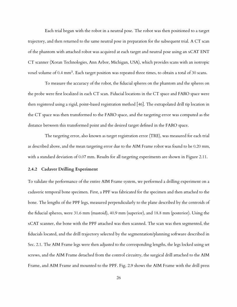
The targeting error, also known as target registration error (TRE), was measured for each trial

as described above, and the mean targeting error due to the AIM Frame robot was found to be 0.20 mm,

with a standard deviation of 0.07 mm. Results for all targeting experiments are shown in Figure 2.11.

2.4.2 Cadaver Drilling Experiment

To validate the performance of the entire AIM Frame system, we performed a drilling experiment on a

cadaveric temporal bone specimen. First, a PPF was fabricated for the specimen and then attached to the

bone. The lengths of the PPF legs, measured perpendicularly to the plane described by the centroids of

the fiducial spheres, were 31.6 mm (mastoid), 40.9 mm (superior), and 18.8 mm (posterior). Using the

xCAT scanner, the bone with the PPF attached was then scanned. The scan was then segmented, the

fiducials located, and the drill trajectory selected by the segmentation/planning software described in

Sec. 2.1. The AIM Frame legs were then adjusted to the corresponding lengths, the legs locked using set

screws, and the AIM Frame detached from the control circuitry, the surgical drill attached to the AIM

Frame, and AIM Frame and mounted to the PPF. Fig. 2.9 shows the AIM Frame with the drill press

26

Patient Number

TargetR

egistratio

nError(m

m)

1 2 3 4 5 6 7 8 9 100.05

0.1

0.15

0.2

0.25

0.3

0.35

0.4Trial 1Trial 2Trial 3

Figure 2.11: Results from free-space targeting trials using the CT phantom. In each trial, the robot wasaimed for drilling to cochlear targets planned for each of the ten patients in the clinical dataset. The trialwas repeated three times, for a total of thirty individual measurements.

attached to the bone.

The trajectory length of 148 mm determined by the control/planning software was then used

to set a mechanical stop on the drill press. A 5/64 inch (1.98 mm) diameter twist drill bit with a 118

point angle was locked into a surgical drill (Anspach Corporation, Palm Beach Gardens, FL, USA).

Drilling was performed at approximately 30,000 rpm, and was completed in 1 min, 26 s. A final CT scan

was acquired of the bone with the PPF still attached and with the drill bit in the drilled hole to evaluate

the drilling performed. In this post-drill CT, the spheres on the PPF were automatically localized and

the drill tip was manually identified. The sphere locations were used to register the pre-drill CT to this

post-drill CT via point registration [46]. The planned trajectory in the pre-drill CT was transformed to

the post-drill CT using this registration. The targeting error, which is the distance between the planned

cochlear target and the drill tip, was determined to be 0.38 mm.

27

drill bit

chorda tympani

facial nerve

ear canal

ossicle

scala tympani

facial nerve

chorda tympani

drill bit

Figure 2.12: Two views of the post-drill CT scan with segmented anatomy and the drill bit that wasguided by the AIM Frame.

2.5 Conclusion and Future Work

In this chapter, we investigated robot-assisted, minimally invasive cochlear implant surgery. Recently,

this surgery has been performed on cadavers using a serial robot that is fixed to the operating room

table [47], however this approach requires an external tracking system and fixation of the patient’s head

to the table. The bone-attached parallel robot approach described in this chapter does not require head

fixation or optical tracking, nor does it require attachment to the operating room table with a rigid and

28

obtrusive frame.

The system we have presented has comparable accuracy to a microstereotactic, but retains the

adjustability of a traditional stereotactic frames. The device simplifies the workflow of microstereotactic

surgery (and specifically PCI surgery), by eliminating the need for a machine shop in the hospital

or alternatively a delay between bone-implanted fiducial placement and surgery to have the fixture

fabricated o site. We believe this elimination of delay and infrastructure will be a key advancement for

widespread deployment of the PCI technique in the future.

However, some additional work is needed before the AIM Frame can be deployed clinically.

We are currently accruing additional clinical trajectories as human microtable cases are conducted, and

we intend to use these to evaluate the necessary workspace of the AIM Frame together with the optimal

number of PPFs. We will statistically evaluate these trajectories to modify the AIM Frame design to

account for patient-to-patient variability in both trajectory orientations and anchor positions. After

concluding this analysis, we intend to perform a clinical evaluation of the AIM Frame, using methods

similar to those presently being used in PCI clinical trials.

We believe that the AIM Frame concept will be advantageous for other intracranial procedures

requiring high positional accuracy. Examples include petrous apex drainage, mastoidectomy, and deep

brain simulation. Some of these (e.g. petrous apex drainage) will be similar to PCI in that they will

involve access to a specific point in image space via a straight-line drill trajectory, and in these an AIM

Frame would work in a conceptually similar way to what we have described in this chapter for PCI.

However, some future procedures (e.g. mastoidectomy and deep brain stimulation) may require that

the AIM Frame be actively moved during surgery to machine bone or realign a surgical tool based on

intraoperative feedback. These examples indicate the potential of the AIM Frame concept to assist with

diverse future clinical tasks in intracranial surgery. Thus we view the initial feasibility study for PCI

29

presented in this chapter to be a first step toward a family of highly accurate, yet adjustable, AIM Frame

guidance fixtures for a variety of intracranial image guided surgical procedures.

30

CHAPTER 3

ROBOTICALLY-ADJUSTABLE MICROSTEREOTACTIC FRAMES FOR

IMAGE-GUIDED NEUROSURGERY

Stereotactic frames are a standard tool for neurosurgical targeting, but are uncomfortable

for patients and obstruct the surgical field. Microstereotactic frames are more comfortable for patients,

provide better access to the surgical site, and have grown in popularity as an alternative to traditional

stereotactic devices. However, clinically available microstereotactic frames require either lengthy manu-

facturing delays or expensive image guidance systems. We introduce a robotically-adjusted, disposable

microstereotactic frame for deep brain stimulation surgery that eliminates the drawbacks of existing

microstereotactic frames. Our frame can be automatically adjusted in the operating room using a

preoperative plan in less than five minutes. A validation study on phantoms shows that our approach

provides a target positioning error of 0.14 mm, which exceeds the required accuracy for deep brain

stimulation surgery. This chapter was presented at the 2013 SPIE Medical Imaging conference [24].

3.1 Introduction

Deep-brain stimulation (DBS) is an FDA-approved treatment for individuals suering from certain

movement disorders that cannot be eectively treated with medications and for treatment of some

aective disorders. Preoperative imaging (MRI or CT) is used to identify a disease-specific target

structure in the brain, e.g., the subthalamic nucleus or globus pallidus interna, and plan an electrode

insertion trajectory. Then, electrodes are surgically implanted. Leads pass from the electrodes out

through the skull under the scalp to a generator under the skin that electrically stimulates the target

structures to alleviate symptoms. Accuracy of 2 mm or better is required when placing the electrodes to

31

achieve eective treatment and to avoid undesirable side eects [48].

The standard guide for implanting electrodes during DBS surgery is the stereotactic frame, a

rigid device surrounding the head and anchored to the skull by sharpened pins penetrating the scalp

and impinging on the skull, as shown in Figure 3.1(a). These devices are heavy and uncomfortable

for patients, a particular disadvantage for DBS surgery in which patients must remain awake during

the procedure to communicate with the surgeon during a two-hour interaction as electrode positions

and voltages are optimized while the eects on symptoms and side-eects are monitored. Stereotactic

frames are aimed by manual adjustment of several vernier scales, which may be aected by human error.

Flickinger et al. [8] found stereotactic frame adjustment errors in 12 percent of 200 clinical cases, and

recommended that two separate observers verify the coordinate settings.

To address the drawbacks of stereotactic frames, two miniature, bone-attached guidance

platforms are now available for clinical use. These “microstereotactic” frames are light and neither

surround the head nor require vernier adjustment. The first is the StarFix microTargeting Platform

(FHC Inc., Bowdoin, ME), shown in Figure 3.1(b), a rigid, lightweight, single-use fixture that is custom-

made by means of 3D printing technology [16] and has experienced exponential growth in clinical use

over the past decade. It is fabricated o-site causing a two day delay between pre-operative imaging and

electrode placement. The second is the NexFrame (Medtronic Inc., Fridely, MN), also a lightweight

guidance device that attaches to the skull [49]. The NexFrame imposes no manufacturing delay, but it

requires an expensive real-time optical tracking system.

An alternative called the Microtable, which combines the advantages of both StarFix and

NexFrame, has been developed at Vanderbilt University for cochlear implantation surgery. Cochlear

implantation surgery requires accuracy of better than 0.5 mm, which traditional stereotactic frames

cannot deliver [49,50]. This fixture also uses bone-attached markers as a reference for targeting a surgical

32

(a) (b)

Figure 3.1: (a) Traditional stereotactic frames are heavy and uncomfortable for patients. These framesrequire manual adjustment, which may lead to targeting errors (image source: Nuclear RegulatoryCommission) (b) Microstereotactic frames, such as the STarFix microTargeting Platform, are custom-manufactured at a special facility, which creates a delay between imaging and surgery.

target in a preoperative CT scan [27]. Like the StarFix, the Microtable is custom-made, but it can be

fabricated in under four minutes on a portable computer numerical control (CNC) milling machine.

Other approaches to making customized fixtures have been proposed. For example, Rajon et

al. [51] developed custom-manufactured biopsy guides for stereotactic neurosurgery. However, each

guide requires three hours to manufacture using a large four-axis milling machine, and it is less accurate

than the Microtable. Kobler et al. proposed a passive Gough-Stewart structure as a drill guide for

cochlear implantation surgery which requires manual adjustment of six micrometers that are attached to

the patient’s head [52]. Thiran et al. introduced an adjustable microstereotactic frame for brain biopsies

and DBS surgery, but this device relies on an external, manually-adjustable stage to aim the device [53].

Robots can perform positioning tasks with accuracy, speed, and precision, and may thus

be beneficial for reducing the time delays and adjustment errors associated with manually-adjusted

stereotactic devices. Bone-attached parallel robots have been proposed for neurosurgical procedures

by Joskowicz et al. [36], and we have developed a bone-attached robot as a microstereotactic frame for

33

cochlear implantation surgery [23]. Robotic frames promise rapid and accurate frame preparation, but

the costs of precision miniature components may be an obstacle to clinical deployment of such devices.

In this chapter, we introduce a microstereotactic frame that is adjusted by a robot, immobilized,

and then attached to a patient for DBS surgery. This approach enables passive frames to be prepared accu-

rately within minutes without manual adjustments, image guidance systems, or lengthy manufacturing

delays.

3.2 Microstereotactic Frame Design

Our proposed microstereotactic frame, which we call the “Freeze Frame”, is shown in Figure 3.2. The

Freeze Frame supports a microTargeting Drive System (FHC Inc.) that advances an electrode into the

brain during DBS surgery. The Freeze Frame comprises a circular plate with four legs that are adjusted

by a robot to align the frame to the correct trajectory and simultaneously to configure the legs for

attachment to four spherical fiducials implanted on a patient’s scalp. DBS electrodes may be implanted in

either hemisphere of the brain. The Freeze Frame is configurable for either left or right hemisphere

implantations.

We designed the Freeze Frame using a set of ten CT scans from patients who underwent

left-hemisphere DBS surgery using the STarFix platform at the Vanderbilt University Medical Center.

We analyzed these CT scans to characterize the range of trajectories and fiducial configurations that

result from variation in both patient anatomy and clinician implantation technique.

The CT scans were processed using WayPoint Planner software (FHC Inc.), which returns

coordinates of the titanium bone anchors (FHC Inc.) that serve as both mounting points and planning

fiducials for the STarFix platform, a vector along the threaded central hole in each anchor, a target point

at the subthalamic nucleus, and an entry point. Additionally, a vector along the anterior commissure-

posterior commissure line was manually identified in each patient CT.

34

FreezeFrame

microTargetingdrive system

(a) (b)

Figure 3.2: (a) The Freeze Frame supports a microTargeting Drive System (FHC, Inc.) that advances anelectrode into the brain during DBS surgery. (b) The frame attaches to four fiducial markers that areimplanted on the scalp.

Like the STarFix system, our system specifies each trajectory by a target point, an entry point

120 mm above the target point, and the anterior commissure-posterior commissure line. The entry

point represents the desired position for the microTargeting Drive System.

To examine the spatial disposition of the bone anchors with respect to each trajectory, we

constructed an orthonormal coordinate frame in each CT scan with an origin at the entry point and

one coordinate axis aligned with the trajectory vector, as shown in Figure 3.3(a). The cross product of

the anterior commissure-posterior commissure vector with the trajectory vector defines the direction

of one additional orthogonal axis which is crossed with the trajectory axis to complete to specify the

remaining orthogonal axis. We then rigidly registered the coordinate frames and transformed all the

spherical fiducial points points to a single coordinate frame located at the entry point origin.

35

electrode trajectory

anchor

spherical fiducial

extender

bone

x y

z

orthonormal frame

(c)

microTargeting Drive Unit

Freeze Frame

(a) (b)

DBS electrode trajectory

Anchor

Spherical fiducial

Extender

Bone

x y

zOrthonormal frame(a)

(a)

(b)

(c)

Figure 3.3: (a) Each patient in our dataset was implanted with four bone anchors for mounting aSTarFix Platform. We propose to add extenders with spherical fiducials for attachment of the FreezeFrame. (b) The STarFix planning software automatically localizes the anchors. We determined wherespherical fiducials would have been located if they were attached to the anchors, instead of a STarFixPlatform. (c) When the spherical fiducials are transformed to a single coordinate frame, their positionsare approximated by a spherical surface. The space of transformed fiducial spheres were used to specifythe dimensions of the Freeze Frame.

The Freeze Frame is designed for mounting to spherical fiducials that were previously developed

for the Microtable [27]. Each spherical fiducial has a threaded extender rod that screws into a STarFix

anchor. To determine where these spherical fiducials would have been located if extender rods were

attached to the anchors on each patient in our dataset, we projected a vector along the central axis of

each anchor, and identified points at the distance from the extender base to center of each sphere. In

the single coordinate frame, all sphere locations lie within 1 cm of a spherical surface found by the

least-squares method, with a radius of 94.5 mm, as shown in Figure 3.3(c). In the Appendix to this

36

chapter, we examine a larger clinical dataset from 1052 DBS surgeries, and find that the fiducials are also

approximated by a sphere for this separate dataset.

The single coordinate frame is convenient for design because all trajectories are transformed to

a single line, with patient variation completely represented by four clusters of fiducial points, as shown

in Figure 3.3(c). By designing a frame in this space with sucient adjustability to reach all fiducials,

the problem of adjusting to each trajectory in the set is solved implicitly without the need to separately

consider trajectory variation.

Four legs provide redundant mechanical support for the circular disc and allow it to be located

with six degrees of freedom. Five degrees of freedom are required to specify the position and orientation

of the trajectory vector, and a sixth degree of freedom is necessary to constrain the angle of an electrode

about its own axis. To achieve this targeting flexibility, each leg mechanism is adjustable for attachment

to a spherical fiducial occupying the three dimensional space beneath the circular disc.

The leg mechanisms are illustrated in Figure 3.4. The legs are seated in a circular track on the

top surface of the circular disc which allows them to rotate about the circumference of the disc. A slot

in each leg supports a block that translates in the radial direction. The sliding block has a cylindrical

hole that serves as a bearing for a shaft that translates in a direction transverse to the plane of the circular

disc and rotates about its own axis. Each shaft is bonded to a foot that supports a gripper mechanism

with a hemispherical cup that mates with a spherical fiducial. The gripper mechanisms were previously

developed for the Microtable [27], and have been validated in cochlear implantation surgery.

The length of each foot provides an oset distance from the shaft axis to the gripper attachment

point, allowing the leg to reach beneath the circular disc. Longer feet are used for the two anterior

fiducial locations. The angle of each foot about the axis of the shaft to which it is attached is fixed during

the adjustment process by a peg that fits into a hole on the bottom of each foot. The foot angles are

37

gripper mechanism

(a) (b)

(c) (d) (e)

footextenderanchorbone

circular track

spherical fiducial

shaft

sliding block

Figure 3.4: (a) Each leg of the Freeze Frame supports a gripper mechanism that fastens to a sphericalfiducial on the scalp. (b) A circular track allows each leg to rotate about the circumference of the circulardisc. (c) a sliding block translates radially in a slot and serves as a bearing for a shaft. The shaft allowsadjustment of the foot height (d) and angle (e).

chosen to align each leg’s range of motion with the expected fiducial positions and to space the legs

evenly about the circumference of the circular disc.

The design of our frame is conservative in the sense that its configuration space is larger than

would be required to reach the ten trajectories in our clinical dataset. As more patient data become

available, we can modify the slot and feet lengths to expand the range of our frame if necessary.

We designed the legs and circular disc to provide manual access to the microTargeting Drive

System and its mounting hardware. No configuration of the legs obstructs access to the thumbscrews or

38

adjustment dials of the Drive System. The thin circular disc also provides a gap underneath the Freeze

Frame for finger access to the incision site. The spaces between the legs provide several inches of lateral

access to this gap.

The Freeze Frame prototype is constructed from Ultem 1000, a biocompatible and autoclavable

thermoplastic (Sabic Innovative Plastics, Pittsfield, MA, USA). The vertical shafts are made of stainless

steel. The coupling ring and gripper mechanisms are anodized aluminum. The total mass of the frame

with the microTargeting Drive System attached is 0.83 kg.

3.3 Microstereotactic Frame Adjustment and Locking

To position the Freeze Frame, we sought a simple, compact, and reliable mechanism. Though all

legs could be simultaneously positioned with independent robot mechanisms, such an arrangement is

unnecessarily complex for our task. Instead, we use a three degree-of-freedom Cartesian robot to adjust

each leg independently. Adjusting the legs separately imposes no significant time delay since only a few

seconds are required for each leg. Since the adjustment robot requires only three motors, we believe it

can be made as compact as a microwave oven.

Prior to adjustment, the Freeze Frame is mounted to two cylindrical pegs that fix the position

and orientation of the circular disc during adjustment. A mounting peg mates with the mechanical

coupling at the center of the Freeze Frame, fitting into the space occupied by base of the microTargeting

Drive and fixing the origin and orientation of the trajectory. A second angular alignment peg fits into a

notch on the circular disc to constrain the angle of the Freeze Frame about the trajectory.

At the beginning of the adjustment process, each leg gripper is unattached. Next, the leg

that will be positioned to the shortest depth beneath the circular disc is fastened to an attachment post.

The attachment post has a spherical top of the same diameter as the spherical fiducials implanted on

the patient, and fits into the hemispherical cup at the bottom of a gripper mechanism. The gripping

39

mechanism is closed around the sphere, so that the cup is fixed on the sphere. The robot then translates

the attachment post such that the vector from the trajectory origin on the circular plate to the attachment

post matches the required vector computed in planning software. As this post is translated, the pieces

that connect the cup to the circular disk slide relative to each other, allowing the cup to remain fixed

while the attachment post translates. After this leg is permanently locked in the correct configuration by

the introduction of a low-viscosity, fast-curing cyanoacrylate adhesive, which rapidly enters the spaces

between the joints by capillary action and forms a very strong bond. The gripping mechanism is then

released, and this procedure is continued for each additional leg in order of increasing height.

At present we require that the gripper mechanisms be manually fastened and released during the

adjustment process, and that the adhesive be manually dispensed into each leg. These manual operations

require less skill than needed for adjusting traditional stereotactic frames. However, we propose two

additional features to fully automate these two operations in future designs, which are illustrated in

Figure 3.5.

First, to automate the fastening and release of the gripper mechanisms, we will provide a

motor-actuated clamp to press the attachment post into the hemispherical cup of a gripper mechanism.

When the Freeze Frame is placed into the robot adjustment chamber, the upper end of each leg shaft

will be inserted into an assigned hole on a plate that is rigidly connected to the mounting peg and

angular alignment peg. A notch on each leg shaft and a corresponding feature in each hole will ensure

that the shafts can be inserted at a specified angle in the correct hole, which will constrain the gripper

mechanisms to known locations within the chamber. The robot can then be programmed to guide the

attachment post to the hemispherical cup of each of the each gripper mechanism and then activate the

clamping mechanism to initiate leg adjustment.

Second, to apply adhesive to the joints, the Freeze Frame will be delivered with a cyanoacrylate

40

dispensing unit attached to the top of each leg. Each dispensing unit will contain an ampoule of 2-

octyl cyanoacrylate. The compound, 2-octyl cyanoacrylate is used clinically as a tissue adhesive (e.g.,

Dermabond) and also bonds mechanical parts with very high strength. After a leg has been adjusted to

the required configuration, a solenoid in the dispensing unit will rupture the cyanoacrylate ampoule with

a sharp pin. Cyanocrylate will flow through a filter to contain the ampoule debris, and then through

multiple nozzles that are aimed at gaps between each leg’s joints. Before the Freeze Frame is attached to

a patient, the dispensing units will be removed from break-away mountings and discarded.

clampingmechanism

cyanoacrylatedispenser

controlwire

end-eectorof 3-DOF robot

planned gripperposition

mountingpeg

sterilepouch

kinematicclamp

kinematicclamp

notch

Figure 3.5: Schematic diagram ofmechanisms proposed for fully automating the Freeze Frame adjustmentprocess and avoiding post-adjustment sterilization.

The Freeze Frame can be sterilized after adjustment, during which it contacts a non-sterile

robot. However, to expedite preparation of the frame, we propose delivering the Freeze Frame in a

41

sterile pouch with features that allow the frame to be adjusted by a non-sterile robot without opening the

pouch until adjustment is complete. The pouch will contain the clamping mechanism and a mounting

peg that mates with the ring on the Freeze Frame that supports the microTargeting drive system, shown

in Figure 3.7(c). The clamping mechanism will be mounted on a metal arm that crosses the boundary of

the pouch through a sealed polymer plate embedded in the flexible pouch material, where the non-sterile

end of the arm will attach to the robot end eector. Similarly, the cylindrical pegs will be mounted on a

second arm that will also cross a sealed polymer plate in the pouch to attach to a stationary point on the

frame of the adjustment robot. To ensure that the circular disc and mounting post are at known positions

within the robot workspace, the mating surfaces between the two arms and the robot will be kinematic

couplings, which can provide positioning repeatability of less than one micrometer [54,55].The two

halves of a kinematic clamp can be held together by an electromagnetic clamp during adjustment.

Electrical control wires for the clamping mechanism and the cyanoacrylate dispensing units will be

routed through the sealed polymer plates.

3.4 Proposed Clinical Workflow

Our proposed workflow for DBS surgery will begin with a preoperative CT scan. A surgeon will

manually select a target point and entry point in three orthogonal views. Prior to surgery, a pre-sterilized

Freeze Frame will be attached to the robot in its sterile pouch.

Surgery will begin with implantation of titanium screw anchors at four locations on the top of

the patient’s skull. We will use FDA-approved anchors manufactured by FHC for the StarFix platform,

and we will add custom extender rods with spherical tips that serve as fiducials [27]. The spherical

fiducials will be localized in an intraoperative CT scan and used to register the preoperatively-planned

trajectory to the intraoperative CT using the mutual information method.

Next, the registered targeting data will be transmitted to the robot, which will automatically

42

adjust and lock the Freeze Frame in the required configuration for guiding electrodes to the chosen

target. The frame will then be removed from its fabrication chamber and securely attached to the

spherical fiducials on the patient, where it will serve as a rigid guidance platform for the duration of

surgery. After surgery, the frame will be discarded.

3.5 Methods

Our experimental dataset consists of fiducial and trajectory data from ten DBS surgeries performed

at the Vanderbilt University Medical Center with the StarFix platform. The data was obtained using

the WayPoint Planner Software as described in Section 3.2 above. The goal of our experiments was to

measure the targeting accuracy of the Freeze Frame after adjustment for each of the ten patients in data

set.

To adjust the Freeze Frame, we used an Exact Jr. 3-axis CNC milling machine (Broussard

Enterprises, Inc., Santa Fe Springs, California, USA) with a Fagor 8040 M CNC controller (Fagor

automation, Elk Grove Village, IL), i.e., a three degree of freedom Cartesian robot, to automatically

adjust each leg. This CNC milling machine is considerably larger and more powerful than required to

adjust our frame, but it can be accurately positioned to ±0.005 mm. We attached a mounting peg and

angular alignment peg to the head of the milling machine to fix the location of the Freeze Frame during

adjustment, shown in Figure 3.6(b).

We embedded four attachment posts in an aluminum plate that was clamped to the mill vise,

shown in Figure 3.6(a). Though our final design will require only one attachment post, we assigned

a separate post to each leg to avoid a milling machine range of motion limitation introduced by the

hardware that we attached to the CNC machine for these experiments.

Prior to all adjustment experiments, the locations of the cylindrical pegs and the spherical

attachment posts were measured using a Faro GagePlus coordinate measuring machine (Faro Technolo-

43

gies Inc., Lake Mary, Florida, USA). To align the measurement coordinate frame axes with the milling

machine translation axes, the Faro device was attached to a pedestal on the bed of the milling machine.

The position of a conical divot mounted to the mill head was measured with the Faro after consecutive

displacements along the three coordinate axes of the milling machine, allowing the Faro’s measurement

frame to be registered to the milling machine’s axes of motion.

(a) (b)

angularalignment peg

mountingpeg

Figure 3.6: (a) The CNC milling machine used to adjust the Freeze Frame during experiments. Thered arrows show the three degrees of freedom of this machine. Attachment posts are embedded in theplate below the Freeze Frame. (b) A cylindrical mounting peg mates with a coupling ring in the circulardisc, and a second peg fits into a notch on the disc to constrain the angle of the Freeze Frame duringadjustment.

To program the CNC milling machine, we wrote a custom Matlab program (Mathworks,

Natick, MA) to automatically generate for each patient G-code (a programming language for CNC

machinery) from the fiducial, target, and entry points obtained from patient CT scans, and from the

peg and attachment post positions recorded with the Faro device. Beginning from a home position,

the program computes the milling machine translations required to position an attachment post at the

planned distance from the trajectory origin defined by the large mounting peg. For each patient, our

program allows us to choose a trajectory length of 110 mm, 120 mm, or 130 mm to provide the shortest

44

distance to the target while maintaining adequate access space beneath the circular disc for the surgeon’s

fingers during the subsequent adjustment process. We selected from these three trajectory lengths

because the same set of fixed lengths are used with the STarFix platform.

To lock the joints of the Freeze Frame, we applied an ethylene-vinyl acetate-based adhesive

(“hot-melt” adhesive) as a substitute for a cyanoacrylate adhesive. Cyanoacrylate adhesives are ideal for

permanent immobilization of the frame but are very dicult to fully remove. Removal of the adhesive

will not be required in practice, because the frame will be discarded after each use, but for our experiments

we reused one frame repeatedly. Though the ethylene-vinyl acetate adhesive provided considerably less

strength and stiness than a cyanoacrylate adhesive would have, the bonds were sucient to hold the

adjusted position of the frame for measurement.

After each frame adjustment, we removed the frame from the robot, fixed it into a vise, and

employed the Faro to measure the centers of the hemispherical cups of the four gripper mechanisms

and then rigidly registered these points to the corresponding planned positions. To find the trajectory

vector of the adjusted Freeze Frame, we measured the interior cylindrical hole of the coupling ring and

a reference surface on the ring using the Faro device. Measurements taken with the Faro are illustrated

in Figure 3.7. The electrode insertion trajectory is aligned with the axis of the cylindrical hole with

an origin at a fixed oset distance from the intersection of the cylindrical hole axis and the reference

surface. Therefore, from the hole and the surface, we could determine the target point in the Faro’s

measurement space by extrapolation. The angle of the trajectory about its own axis is indicated by a

reference divot on the coupling ring, which was also measured with the Faro device.

A rigid transformation was determined that placed the centers of the hemispherical cups as

measured in Faro space onto the centers of the fiducial spheres as measured in CT space with least-squares

error [56]. For each patient, we transformed the target position in the Faro measurement coordinate

45

(a) (b) (c)

Faro ball probe

cylindricalhole

referencedivot

reference surface

Figure 3.7: After the Freeze Frame was adjusted to a patient trajectory, a Faro portable coordinatemeasuring machine was used to measure features on the frame. (a) The four hemispherical cups of thefiducial gripper mechanisms were measured with a ball probe that was attached to the Faro. This probewas also used to measure features on the electrode driver coupling (b),(c). These features were used tofind the position and orientation of the electrode trajectory.

frame to the corresponding space of planned points, and subtracted the planned target from the measured

target to obtain the fabrication error at the target, et. The root mean square of et is calculated from the

mean et and standard deviation σt of et:

RMS(et) =√et2 + σ2

t (3.1)

The target registration error (TRE) of the Freeze Frame depends on et and the fiducial localization

error in image space. We estimate the root mean square value of fiducial localization error in image

space, 〈FLEimage〉, to be 0.11 mm. This estimate was obtained from CT scans of a phantom embedded

with the same spherical fiducials used with the Freeze Frame [57]. For the ith patient, we calculated the

expected TRE due to image localization error, 〈TREFLE(i)〉 from both the particular configuration of

fiducials implanted on that patient and our estimate for 〈FLEimage〉 [58]. The mean squared value of

46

〈TREFLE〉 for our dataset is given by the following:

⟨TRE2

FLE

⟩=

1

10

10∑i=1

⟨TRE2

FLE(i)⟩

(3.2)

By adding Equations 3.1 and 3.2 in quadrature, we calculate the expected value of the root mean square

TRE of the Freeze Frame using Equation 3.3:

〈RMS(TRE)〉 =

√RMS2(et) +

⟨TRE2

FLE

⟩(3.3)

We obtained the fabrication error in the angle of the trajectory about its own axis (henceforth called

the “angular fabrication error”), ea, by transforming the measured position of the angular reference

divot to the space of planned points and comparing it to the planned position of the divot. The mean

and standard deviation of ea are calculated using the directional versions of these statistics [59]. The

accuracy of this angle determines the accuracy of adjustments made during the surgical procedure to the

position of the electrode in response to changes in patient symptoms and side eects during stimulation.

In particular, when adjustments are made in a direction perpendicular to the trajectory, an error in

the angle will cause the actual adjustment to be dierent from the desired adjustment. Because of the

limitations of the electrode driver, the maximum distance of adjustment perpendicular to the trajectory

is 5 mm. The maximum error in electrode placement resulting from an adjustment of length r, when

the angular error is ∆θ, is equal to 2r sin(∆θ/2) radians. As pointed out above, the maximum error

in electrode placement is 2 mm. Inverting our expression for the maximum error for a given ∆θ, we

find that the maximum acceptable angular registration error, ea, is equal to 2 sin−1(2 mm/(2× 5 mm)),

which equals 0.4 radians or 23 degrees (we are omitting the contribution of the angular error resulting

from fiducial localization error, because the error is approximately equal to FLEimage divided by the

47

mean distance between fiducials : 0.11 mm/123.6 mm = 0.0009 radians, which is about 0.05 degrees and

is thus negligible.). We will consider ea values that are at least one order of magnitude below 23 degrees

to be acceptable.

3.6 Results

The results of the ten trials are summarized in Table 3.1. For all trials, the estimated target registration

error were an order of magnitude lower than the maximum 2 mm error considered acceptable for

DBS stimulation surgery. The angular fabrication error had a maximum absolute value of 0.08 degrees

(1.42× 10−3 radians), which is also much smaller than the maximum of 23 degrees that we consider to

be acceptable.

Table 3.1: The estimated target registration error and angular fabrication error for all ten trials werewithin safe limits for DBS surgery. Maximum values are indicated by bold text. The patient numbersindicate to the order in which the trials were performed.

TrajectoryLength (mm)

TargetFabricationError (mm)

AngularFabricationError (deg)

Estimated TargetRegistration Error

(mm)

Patient 1 120 0.06 0.055 0.13Patient 2 120 0.08 -0.034 0.13Patient 3 120 0.15 0.009 0.18Patient 4 110 0.12 0.081 0.16Patient 5 120 0.09 -0.041 0.14Patient 6 120 0.22 0.044 0.24Patient 7 120 0.14 -0.034 0.17Patient 8 110 0.14 -0.023 0.17Patient 9 130 0.11 -0.018 0.15Patient 10 130 0.24 -0.033 0.26

Root Mean Square 0.14 0.042 0.18Mean 0.13 0.001 0.17Standard Deviation 0.06 0.042 0.04

48

3.7 Conclusions

We have described a rapidly-adjustable microstereotactic frame for guiding intracranial targeting and

a validation that provides sucient targeting accuracy for DBS surgery. We have also introduced a

method for analyzing clinical data to specify the design of this frame, and have demonstrated a method

for adjusting a frame with six degrees of freedom using only a three degree of freedom robot.

Previously, we developed a model to predict the eects of external forces and torques on target

registration error [57] and plan to apply this model to the Freeze Frame in our future work. We expect

to find that that the small external forces and torques during surgery will contribute an insignificant

amount to the target registration error.

In this study, we considered only DBS surgery, but we also plan to explore the suitability of

the Freeze Frame for other stereotactic procedures, including biopsies, pallidotomies, thalamatomies,

shunt placement, and otologic procedures.

49

CHAPTER 4

MEASUREMENT AND PERCEPTION OF TRAUMATIC FORCES IN COCHLEAR

IMPLANTATION SURGERY

Tissue trauma is known to occur frequently in cochlear implantation (CI) surgery, but the

relationship between force, trauma, and surgeon’s perceptual capabilities is poorly understood. In this

chapter, we consider translocation of cochlear implant electrodes from the scala tympani (ST) to the

scala vestibuli (SV), which occurs frequently and may lead to suboptimal audiologic outcomes. Fresh

(postmortem < 120 h), nonfixed, never-frozen human temporal bones were prepared by surgically isolat-

ing the cochleae and exposing the osseous spiral laminae, basilar membranes, and Reissner’s membrane.

Each isolated cochlea was mounted to a force sensor using a poseable mounting platform and punctured

with a probe while concurrently recording forces and video. The mean force at rupture was 88 mN, and

ranged from 42 mN to 122 mN.

The perceptibility of rupture or other forces during CI surgery has not been studied. We

introduce a psychophysical testing procedure to estimate the threshold of perceptible force in CI surgery.

Semmes-Weinstein Monfilaments (SWM) are a standard clinical tool for quantifying tactile sensation.

We adapt these tools as a model of a grasped CI forceps, and use a two-alternative forced choice, staircase

procedure to measure force perception of ten otolaryngological surgeons (six residents, four attending).

We measure a mean threshold of 21 mN, which suggests that rupture forces are perceptible under some

circumstances. The contents of sections 4–4.4 of this chapter were accepted for publication in Otology &

Neurotology.

50

4.1 Introduction

Cochlear implantation (CI) is the standard of care for severe to profound sensorineural hearing loss. Rapid

progress in technology, from its inception in 1957 to U.S. Food and Drug Administration approval in

1984 to current multichannel devices with modern processing techniques, has led to a dramatic increase

in the number of patients who have benefitted from this technology [60]. Despite overwhelming success,

CI is not without complications. Estimates of complication rates in the literature range from 4 percent

to 40 percent [61]. One major subset of complications involves problems associated with CI electrode

insertion. In unusual cases, insertion of the electrode is not feasible because of anatomic considerations.

In most other instances, electrode insertion is not perceived to be dicult but damage to intracochlear

structures inadvertently occurs, potentially resulting in suboptimal hearing outcomes for patients.

The surgical technique for CI is typically via a standard mastoidectomy with facial recess

approach to the middle ear. This is followed by entering the cochlea, either via the round window or a

separate cochleostomy, and inserting an electrode array. The goal is to insert the array into the scala

tympani (ST) without damage to intracochlear structures. One major challenge is poor visualization.

The surgeon is able to visualize the cochleostomy itself, but intracochlear structures, such as the osseous

spiral lamina (OSL), Reissner’s membrane (RM), and the basilar membrane (BM), are only partially

visible via the cochleostomy, with the vast majority of the structure hidden by bone. The surgeon thus

performs the critical step of the procedure blind to intracochlear anatomy and guided mainly by tactile

feedback.

Translocation of the CI electrode array from the ST to the scala vestibuli (SV) with resultant

intracochlear damage represents one cause of suboptimal hearing outcomes in patients undergoing CI.

Multiple groups have documented poorer hearing outcomes should the electrode array cross from the

51

SV

ST

LCW LCW

indenter

indenter

ST

SV

(A) (B)

Figure 4.1: Cochlear schematic. (A) Cross-section of a right cochlea, with an indenter probe enteringthe scala tympani (ST) approximately 90 degrees along the basal turn. The schematic in the foregroundshows the interscalar partition (black arrow) exposed from below (bone underlying ST has been drilledaway) and above (removal of bone overlying the scala vestibuli [SV] is shown). LCW indicates lateralcochlear wall. (B) Orientation of cochlear specimen used during experimentation, which is upside down(flipped 180 degrees) from anatomic orientation, such that ST is above SV.

ST to the SV [62–65]. Although data exist comparing histopathologic changes of the cochlea with

varying insertion depths of CI electrodes [66], there are limited data estimating the amount of force

required for such translocation. The most relevant prior experimental results were reported by Ishii et

al. [67], who used a blunt needle to puncture the round window (RW), BM, and RM, each of which

was explanted from a single adult cochlea. The authors reported a BM rupture force of approximately

30 mN. The single RM tested had a rupture force of 4.2 mN. We propose to treat the OSL, BM, and

RM as one entity because most clinical translocations completely traverse from the ST to the SV, often

involving damage to all three structures. In doing so, we preserve the anatomic attachments of this group

52

of structures, which we refer to collectively as the interscalar partition, to both the lateral and medial

cochlear walls, which we hypothesize provide significant structural support. In addition, we sought to

develop a technique that could be used on multiple temporal bones to assess interspecimen variability.

In most circumstances, electrode insertion is not perceived by the surgeon to be dicult.

However, the relative ease with which most electrode arrays are inserted does not guarantee that this

portion of the procedure is carried out without undesired intracochlear trauma. In particular, damage to

the cochlea can occur even in the absence of perceived diculty with electrode insertion by the surgeon.

This potentially results in suboptimal hearing outcomes for patients. In Section 4.5, we shift the focus of

this chapter from the cochlea to the surgeon, and investigate the threshold of force perceptibility.

4.2 Materials and Methods

Twelve human temporal bones (six left, six right) were acquired from a tissue-harvesting service (Science

Care, Phoenix, AZ, USA). The temporal bones were harvested immediately postmortem, stored in saline,

and shipped cooled, but not frozen. All experimentation was carried out with bones no greater than

120 hours postmortem. Specimens were first prepared by isolating the cochlea without violating any

intracochlear structures. This was achieved using the following dissection technique:

1. Perform a canal wall down mastoidectomy, including removal of the incus and malleus and sacrifice

of the chorda tympani nerve.

2. Perform a labyrinthectomy.

3. Isolate the superior aspect of the cochlea by removing the horizontal (tympanic) segment of the

facial nerve and all bone superior to it with a 4 mm cutting drill bit.

4. Isolate the anterior aspect of the cochlea by drilling into the carotid artery and removing all bone

anterior to it.

53

(B)

indenter tip

poseable

piezoelectric motor

acrylic frame

force sensor

(A)

stage

platform

Figure 4.2: Experimental apparatus. (A) A sturdy acrylic frame supports a force sensor and piezolectricmotor. The piezoelectric motor advances in the direction of the arrow to contact the specimen, whichrests on a stage attached to the force sensor. (B) An enlarged view of the indenter, which is tipped witha 300 µm-diameter ruby sphere. The poseable mounting platform allows the specimen to be orientedsuch that the scala tympani is positioned just below the probe, with the basilar membrane, osseous spirallamina, and Reissner’s membrane approximately perpendicular to the insertion axis.

5. Isolate the cochlea from bone posterior to it by drilling away the pyramidal eminence, sinus

tympani, and vertical (mastoid) segment of the facial nerve.

6. Using hypotympanic air cells as an inferior landmark, cut away all remaining temporal bone with

a diamond band saw (Gryphon Corp, Sylmar, CA, USA), leaving an isolated cochlear specimen.

After the cochlea was isolated, a combination of microdissection instruments and 1 mm diamond

drill bit were used to manually expose the interscalar partition in the area approximately 90 degrees along

the basal turn of the cochlea. Care was taken to leave labyrinthine bone in place between the round

54

ruby ball

interscalar partition

scala tympani

scala vestibuli

Figure 4.3: Orientation of experimental setup. Left cochlear specimen showing orientation of indenterto the interscalar partition before rupture. Bone between round and oval windows in this specimenhas been removed to demonstrate the anatomy (pilot experiments, not included in data collection oranalysis). The interscalar partition can be seen dividing the cochlear chambers into scala tympani aboveand scala vestibuli below. The indenter moves in the direction of the green arrow.

and oval windows as a supporting structure. In addition, bone was left in place at the lateral cochlear

wall. Bone overlying the ST and the SV was removed under microscopy using a 1 mm diamond burr to

expose the interscalar partition from above and below, as illustrated in Figure 4.1.

55

lateral cochlear wall

oval window

labyrynthine bone

round window (approximate location)

indenter

Figure 4.4: Right fresh human cochlear specimen before rupture, viewed from the scala tympani.The indenter is positioned directly above the interscalar partition, which is supported by native bonyattachments. The dashed line indicates the approximate round window (RW) region before removingthe RW niche and the RW membrane.

The experimental apparatus, shown in Figure 4.2, consisted of a custom-built, rigid acrylic

frame. A Nano-17 force sensor (ATI Industrial Automation, Apex, NC, USA), was mounted to the base

of the frame, and a small stage was attached to the force sensor to support cochlear specimens. The

force sensor had a resolution of 1/320 N and was factory calibrated immediately before the experiments.

Each specimen was fixed with epoxy to a custom-built poseable mounting platform, which was placed

on the stage. The platform was adjusted such that the surface of the interscalar partition that faces the

ST was approximately orthogonal to the insertion axis, and then the mounting platform was locked

56

by application of cyanoacrylate adhesive. In the experimental position, ST was immediately below the

puncture probe and oriented above the SV. An SL-2060 piezoelectric linear motor with a displacement

resolution of 1 µm (SmarAct GmbH, Oldenberg, Germany) was attached to the frame and was used

to advance a rigid probe with a 300 µm diameter coordinate measurement machine ruby ball probe

(itpstyli, St. Louis, MO, USA), which was aligned with a single axis of the force sensor. With the

aid of an operating microscope (Carl Zeiss AG, Oberkochen, Germany), the specimen was manually

positioned directly underneath the tip of the probe, such that they were oriented orthogonal to the

insertion axis. The probe was advanced until it was approximately 200 µm from the tissue surface, as

shown in Figures 4.3 and 4.4. The probe was then advanced at a velocity of 1 mm/s from the ST to the

SV while concurrently recording force from the load cell and videomicroscopy of the rupture, as shown

in Figure 4.5.

(A) (B)

LCW LCW

LB LB

Figure 4.5: Right fresh human interscalar partition before and after rupture, viewed from scala vestibuli.Prerupture (A) and postrupture (B) view of the specimen. The bony structural support can be seen oneither side of the interscalar partition. LCW indicates lateral cochlear wall, and LB indicates labyrinthinebone between the round and oval windows. Note that the ruby ball punctures the interscalar partitionwithout detaching it from the surrounding bone.

57

Custom software written in the C programming language was used to simultaneously control

the motor and record data. The program was executed on a 2.66 GHz Intel Xeon processor running

an Ubuntu 12.04 Linux operating system that was configured for real-time operation. The data were

sampled at 5000 Hz and filtered using a fifth-order zero-phase Butterworth filter with a cuto frequency

of 25 Hz. The peak puncture forces were estimated by calculating the absolute maximum value in each

filtered data set. In addition, each video was reviewed to determine the type of rupture that occurred.

These were classified as either punctures or avulsions. A puncture was defined as the ruby ball penetrating

from the ST to the SV without tissue detachment from the lateral or the medial support, whereas an

avulsion was defined as a detachment from either the lateral or the medial bony attachments without

puncturing.

4.3 Results

Twelve temporal bones were obtained and prepared. A total of ten bones were included in the final

analysis. One of the excluded specimens was damaged during preparation and was not analyzed because

of its lack of structural integrity at the time of testing. In the second excluded specimen, the probe

was inadvertently advanced into the labyrinthine bone below the SV during experimentation, causing

a very large spike in force measurements from which we were unable to isolate the rupture forces.

Consequently, this specimen was excluded from the final analysis.

Force recordings for the ten analyzed bones are shown in Figure 4.6. Nine of the ten specimens

demonstrated an approximately linear increase in force, followed by a rapid release of force noted

immediately after puncture of an elastic surface. In one specimen, an avulsion from the medial wall

occurred. The rupture forces ranged from a minimum of 42 mN to a maximum of 122 mN, with a mean

of 88 mN and a sample standard deviation of 25 mN.

58

Distance (mm)

Force(m

N)

0 0.25 0.5 0.75 10

50

100

Distance (mm)

Force(m

N)

0 0.25 0.5 0.75 10

50

100

Distance (mm)

Force(m

N)

0 0.25 0.5 0.75 10

50

100

Distance (mm)

Force(m

N)

0 0.25 0.5 0.75 10

50

100

Distance (mm)

Force(m

N)

0 0.25 0.5 0.75 10

50

100

Distance (mm)

Force(m

N)

0 0.25 0.5 0.75 10

50

100

Distance (mm)

Force(m

N)

0 0.25 0.5 0.75 10

50

100

Distance (mm)

Force(m

N)

0 0.25 0.5 0.75 10

50

100

Distance (mm)

Force(m

N)

0 0.25 0.5 0.75 10

50

100

Distance (mm)

Force(m

N)

0 0.25 0.5 0.75 10

50

100

Figure 4.6: Forces recorded during translocation of test probe from scala tympani to scala vestibuli. Peakforces are identified by a dashed red line.

59

4.4 Discussion

Our measurements of the forces required to translocate a test probe from the ST to the SV have significant

clinical implications regarding CI surgery. Our test probe results are comparable to translocation of

electrode arrays. This represents perhaps the largest avoidable cause of failure to maintain residual hearing,

which has been shown to impact audiologic outcomes even in patients with little to no serviceable

preoperative hearing [68]. Before the work presented herein, there were few published results from

which to estimate unsafe forces during CI electrode array insertion. This information is useful as systems

and techniques for CI electrode array insertion are refined, including robotic systems that could be

programmed to insert electrodes up to a given force level below which intracochlear trauma would be

unlikely to occur.

To our knowledge, this is the first report of measured rupture forces associatedwith translocation

from the ST to the SV in situ (i.e., tissues left attached to their native bony attachments). Whereas

Ishii et al. [67] have previously performed experimentation to calculate the mechanical properties of

isolated human BM tissue, these experiments evaluated a single fixed and explanted specimen, divided

into three separate samples from dierent regions of the cochlea. This tissue lacked the in vivo support

that would resist the forces applied by an electrode during CI surgery, as it was fixed and explanted. To

overcome this limitation, we have developed a novel method of cochlear preparation in which the OSL,

BM, and RM of the cochlea are exposed approximately 90 degrees along the basal turn while maintaining

attachments to the medial and lateral cochlear walls. In addition, we performed the experiments on a

larger sample size (n = 10). The mean rupture force was 88 mN, supporting our hypothesis that the OSL,

BM, and RM complex, complete with native lateral and medial attachments, would have a larger rupture

force than ex vivo BM as tested in the 1995 study [67].

60

The experimental setup was designed to replicate the conditions relevant to puncture of the

interscalar partition. One aspect of this was the choice of the indenter used. The diameter of the

ruby ball-tipped indenter was 300 µm, which is similar in size to that of a CI electrode array tip. In

addition, its rounded shape eliminates the sharp edge used in prior work [67], which could cut tissue,

potentially falsely reducing the forces necessary to rupture it. The hard spherical indenter also provides a

well-defined contact condition for each trial. To mimic the in-vivo tissue as closely as possible, we used

fresh, less than 120 hours postmortem, tissue that was not fixed and had never been frozen. In addition,

we developed a method of exposing the OSL, BM, and RM complex approximately 90 degrees along the

basal turn from both the ST and the SV without disrupting its native bony attachments, allowing us to

closely simulate the clinical scenario of CI.

Although the work described here represents an important step in obtaining a better under-

standing of clinically relevant intracochlear trauma, more work is necessary to further characterize it.

Our work investigated normal forces (i.e., those perpendicular to the interscalar partition) exclusively to

faithfully replicate the rupture phenomenon and to characterize one fundamental type of loading. It is

hypothesized that clinical damage often occurs when the electrode array is deflected o the walls of the

ST in the basal turn, approximately 180 degrees from the insertion site, during which we believe normal

forces predominate. However, over the full length of insertion, punctures may occur at various angles

to the interscalar partition, and an understanding of the mechanisms of trauma may be improved by

investigation of combined normal and tangential loading at dierent locations along the cochlea in the

future.

As CI surgical techniques continue to improve, automated electrode insertion may hold the

potential to minimize trauma by inserting at a slow regulated velocity and stopping or altering the

insertion trajectory when real-time force feedback indicates forces high enough to cause trauma, for

61

example, translocation from the ST to the SV. Our group has studied robotic insertion and has shown

that electrodes inserted robotically have significantly less variation in force than those inserted by human

operators [69]. Furthermore, preliminary data on electrode insertion forces generated during robotic

insertion demonstrate significant dierences between standard insertion techniques and those guided

by stylets to avoid collision with the cochlear walls [70]. Before the work described herein, the clinical

significance of these findings was speculative at best. We conclude that minimizing insertion forces will

reduce the risk of translocation of a CI electrode array and lead to improved audiologic outcomes. Our

data suggest that an average of 88 mN is required for such translocation to occur, but they can occur

with forces as low as 42 mN. This leads to perhaps the most perplexing question generated by these data

can human surgeons perceive such forces? This question will be addressed in the following section.

4.5 Measurement of surgeon force perception thresholds in cochlear implantation

Insertion forces are not recorded during cochlear implantation surgery. Rather, they may or may not

be perceived by a surgeon, who alone decides whether or not corrective action should be taken to avoid

damaging the cochlea. To date, no study has investigated surgeons’ ability to perceive insertion forces

during CI surgery. There is a fundamental diculty in measuring perceptual thresholds: they relate

to mental states which cannot be directly observed. In this section, we adapt methods from the field of

psychophysics to the problem of measuring surgeons’ tactile thresholds.

Psychophysics studies the relationship between stimuli and the perceptibility of those stimuli [71,

72]. The study of perceptual thresholds began with the work of Fechner and Weber in the 19th

century [73], and has evolved into the testing procedures that are routinely used in audiometry and

optometry, for example.

In modern psychophysics, perception is viewed as a probabilistic process in which the ability

to perceive a fixed stimulus intensity varies with repeated application of the stimulus. Perception is

62

understood to occur in the presence of noise, including both external noise and the intrinsic noise of

the sensory system. As the intensity of a stimulus increases, the signal to noise ratio increases, and the

probability of correctly identifying the stimulus gradually increases according to a relationship described

by a psychometric function. Psychometric functions vary in shape according to the sensory modality and

nature of the stimulus. A typical psychometric function in illustrated in Figure 4.7 with contrived data.

A threshold can be chosen as a stimulus intensity (on the abscissa) corresponding to a certain percent

correct level on the curve, such as the level at which 50 percent of the stimuli are correctly identified.

Thus, a threshold is not a sudden step change from “not perceivable” to ‘’fully perceivable”, but is rather

a quantity derived from the psychometric function.

stimulus intensity

percentcorrect

1 3 5 7 9 11 130

50

100

psychometric function

experimental data

Figure 4.7: A psychometric function relates the intensity of stimuli to performance at a psychophysicaltask. The function can be estimated by fitting a curve to percent correct data at multiple stimuli level,but estimation of a single threshold stimulus is more eciently estimated by an adaptive method. In thecontrived example shown here, the 50 percent threshold corresponds to a stimulus intensity of 7.

A psychometric function can be approximated by fitting a curve to response data measured

over a range of stimulus levels, but this approach requires a large number of trials and is inecient

and tedious if only a threshold value is desired. An alternative is to use one of several adaptive testing

63

procedures, which adjust stimulus intensities according to correct or incorrect responses in order to

eciently target the data needed for computation of a threshold. In this study, we will use a staircase

adaptive procedure [74, 75]. Staircase trials begin with a large, easily perceivable stimulus intensity,

which is reduced by fixed increments until a participant responds incorrectly. Following the incorrect

response, the stimulus intensity is increased by graduated increments until the participant response

correctly, at which point the direction of increment is again reversed. The threshold is estimated by

averaging the reversal points. Often, an “n-down-1-up” rule is used in which n successive correct

responses are required before the stimulus can be decreased. The convergence properties of staircase

procedures depends on the stimulus intensities, step sizes, number of trials and other factors, and are

rigorously examined by Garcia-Perez [76]. Generally, adaptive procedures do not target the 50 percent

level on the psychometric curve. The three-down, one-up design that we will use in this study converges

on the 79.4 percent correct level [77], for example.

Results from psychophysical experiments are prone to errors caused by several cognitive biases.

For example, participants may arm the presence of a stimulus even when it is absent or below the actual

threshold from a desire to perform well. This bias is of particular concern in the present study, because

success at the experimental task may be interpreted as an indicator of occupational skill. A standard

method to eliminate bias in psychometric trials is the two-alternative forced choice (2AFC) method.

Rather than replying “yes” or “no”, a participant is forced to choose between randomly assigned noise

and stimulus alternatives.

There is a large body of psychophysical research relating to the hand and fingertips [78,79],

but few studies have examined absolute force perception thresholds under conditions comparable to CI

insertion. Force thresholds have been measured in the context of diabetic neuropathy testing [80,81],

but the point forces applied in neuropathy testing do not resemble the distribution of pressure across

64

a surgeon’s gloved palm and fingertips. Loads distributed across one or more fingertips have been

tested by developers of haptic devices. Dosher and Hannaford used a forced-choice, adaptive testing

protocol to measure forces applied to the fingertip with a haptic device [82], and reported average

detection thresholds ranging from 30.1 mN to 50.4 mN. Using a similar pyschophysical testing protocol,

King, Donlin, and Hannaford [83] applied forces to multiple combinations of fingertips, and reported a

threshold range of 27.8 mN to 34.0 mN. Baud-Bovy and Gatti transmitted force via a robot end eector

to a spherical handle grasped by a subject, and reported a minimum threshold of 49 mN when subjects

were allowed to move the handle to seek the direction of the force [84]. These studies advance our

understanding of the hand’s sensitivity, but the configurations of these devices did not resemble the

grasp and motion used in CI surgery.

In this study, we will test the force perception thresholds of a group of surgeons using equipment

designed to replicate the arm posture and forceps grasp used in CI surgery, using an adaptive staircase

psychophysical testing procedure.

4.5.1 Methods

Twelve participants were recruited via email, phone, and personal communications. Inclusion criteria

stipulated that all research participants must be otolaryngologists who actively perform CI surgery

in their clinical practice, or otolaryngology residents at a residency training program approved by

the Accreditation Council for Graduate Medical Education (ACGME). Postgraduate year 1 (PGY-1)

residents were excluded, as they have little to no training or experience in otologic surgery at this stage of

residency. Six participants were current residents or fellows at the time of testing, and four had completed

training and were practicing surgeons. Additional demographic information is shown in Table 4.5.1. All

participants signed informed consent after reviewing the risks and benefits of participation. This study

was approved by the Vanderbilt University Institutional Review Board.

65

Resident/Fellow Attending

GenderMale 6 4Female 0 0

Average Age (years) 29.67 55.0Fellowship Training Completed

Otology/Neurotology n/a 3Pediatrics n/a 1

Performs CI in Clinical Practice n/a 4Mean Number of CI Surgeries per Month n/a 5.25Handedness

Right 6 4Left 0 0

Table 4.1: Demographics of participants included in analysis of force perception thresholds.

To apply forces reliably andwith known intensities, we used Semmes-WeinsteinMonofilaments

(SWM). These devices consist of a handle with a nylon monofilament tip that is calibrated to buckle at a

particular force. SWMs are a standard clinical tool for cutaneous sensory function, and are used regularly

to evaluate diabetic peripheral neuropathy. They are recommended by the World Health Organization

as devices that can be used by health professionals for repeatable testing and measuring of the threshold

of cutaneous sensory perception [85], and their mechanical reliability has been rigorously evaluated [86].

In clinical usage, a physician grasps the SWM handle and presses the filament tip into a patient’s

skin until the filament buckles. To replicate electrode insertion in our experiments, participants held an

SWM handle between the thumb and index finger to model the grasp of CI forceps. By buckling the

filament, the calibrated force was applied to participants’ hands in a way that resembles the transmission

of force through CI forceps (we shall describe how the filaments were buckled shortly).

SWM filaments are manufactured in a standard set of buckling strengths. These buckling

strengths increase on an approximately logarithmic scale [87]. A logarithmic scale is used because the

perceived intensity is approximately linear with logarithmic increase of force. We selected a set of eight

66

SWM force intensities, listed in Table 4.2, to span the estimated perceptual range of participants.

Table 4.2: Semmes-Weinstein monofilaments were selected from the standard clinical set to span theexpected range for the force threshold during CI surgery.

Force (g) Force (mN)

0.4 3.90.6 5.91 9.81.4 13.72 19.64 39.26 58.88 78.510 98.115 147.1

We constructed a fixture, shown in Figure 4.8, to cause SWM filaments to buckle reliably over

multiple trials and to reduce variability in the motion of the SWM handles among participants. In the

intended clinical use of SWMs, a physician moves the handle and visualizes buckling of the filament

as it is pressed into a patient’s skin. The SWM is shielded from participants’ view in our experiments,

so the fixture constrains the handle to move between two fixed endpoints. Before commencing a trial,

the SWM handle is placed in a starting fixture, shown in Figure 4.8(a), that suspends the filament tip

above a target surface. The distance between the starting fixture and the target surface is fixed, but

the mutual height of these components above the tabletop is adjustable. The experimenter adjusts this

height, as shown in Figure 4.8(b), such that the SWM handle is approximately parallel to the tabletop

when held in the starting fixture. Without a means to adjust the height of the starting fixture, the SWM

handle would be initially inclined with respect to the target surface at an angle that is propotional to a

participant’s palm width. Such initial angulation of the handle is undesirable as it biases the filament to

contact the target surface at a steep angle and possibly skid or bend rather than buckle. To commence

a trial, the experimenter pulls a handle to release the SWM handle from the starting fixture, as shown

67

in Figure 4.8(c). The participant then lowers the handle until it contacts a stopping plate, in which

position the filament is buckled, as shown in Figure 4.8(d). The height of the stopping plate was chosen

to be slightly shorter than the average filament length amongst the SWM devices tested in order to stop

advancement just after buckling, preventing extreme bending or slippage of the filament on the target

surface.

handle

target surface

experimenter

participant

monofilament

(a) (b)

(c)

(d)

startingfixture

stoppingplate

adjustmentknob

Figure 4.8: (a) A custom-built testing device used to model the advancement of forceps and transmissionof electrode-basilar membrane contact forces during cochlear implantation surgery. In each trial, aparticipant lowers a Semmes-Weinstein Monofilament (SWM) handle from the starting fixture untilit contacts the stopping plate. If a monofilament is attached to the SWM handle (control trials omitthe monofilament), the monofilament will buckle against the target surface when the handle contactsthe stopping plate, causing a calibrated force to be applied to the participant’s hand. (b) Before testing,the device is adjusted to the height of each participants’ hand, such that the initial orientation of theSWM handle is approximately parallel to the tabletop (c). To begin each trial, the experimenter placesthe SWM handle in the starting fixture, which is at a fixed height above the stopping plate and targetsurface. The experimenter then retracts the starting fixture and instructs the participant to lower theSWM handle. (d) The handle rests on the stopping plate at the end of each trial.

Tracey, Greene, and Doty performed experiments to evaluate the test-retest reliability of

68

two alternative forced-choice (2AFC) staircase procedures for SWM testing of tactile thresholds, and

recommended a three-down, one-up (3D1U) rule for reversals [88]. The authors found that a test-retest

reliability coecient greater than 0.80 could be achieved with as few as two reversal pairs. Encouraged

by these results, we adapt the 2AFC-3D1U psychophysical testing procedure recommended by Tracey

et al. for our model of CI surgery.

Participants were seated behind an opaque curtain, shown in Figure 4.9, to prevent observation

of the testing apparatus and of the experimenter. Each participant donned an appropriately sized surgical

glove on the dominant hand and passed this hand through a slit in the curtain, which was covered by an

additional flap of fabric to prevent observation through the slit.

curtain

(a) (b)

curtainframe

additionalflap

monofilamenthandle

testingdevice

dominanthand

Figure 4.9: (a) An opaque curtain is placed between participants and the testing device to prevent visualobservation of the experimental apparatus and experimenter during trials. The curtain ensures thatparticipants experience only tactile feedback by avoiding visualization of either Semmes-Weinsteinmonofilament (SWM) buckling during experimental trials, and also obstructs visual observation of SWMhandles without attached monofilaments during control trials. (b) A top view of a seated participant.The participants’ dominant hand is inserted through a hole in the curtain, which is covered with anadditional flap of curtain fabric to prevent visualization through the opening in the main curtain. Theexperimenter (not shown) sits opposite to the participant. The curtain prevents the participant fromvisually observing the experimenter, who reads instructions to the participants from a prepared script.

Before commencing trials, each participant was read instructions from a prepared script which

69

is included in the Appendix to this chapter. To implement paired 2AFC trials, one SWM device was

modified by removing the filament entirely (a negative control). Each trial consisted of a pair of handles,

one with a standard SWM and the other with the modified control handle, in a random order. The

experimenter placed a SWM handle (either a filament or the negative control) in a participant’s hand,

and then guided the handle to rest in the starting fixture. Next, the experimenter retracted the starting

fixture and read a scripted notice to the participant to begin lowering the SWM handle. The participant

was then instructed to advance the SWM handle straight downward at a speed that he would normally

use to insert a CI electrode array, until the SWM handle contacted the stopping plate. This sequence

was then repeated with the second half of the pair (either a filament, or the negative control). Following

a 2AFC trial, participants were instructed to report which device (the first or the second) contained the

filament.

We implemented a 3D1U staircase testing procedure beginning with a filament buckling

strength of 39.2 mN which we believed would be 100 percent perceivable by all participants. After

three consecutive correct 2AFC trials, the filament strength was decreased by one increment in the

series of filaments. Conversely, an incorrect response, implying an inability to perceive the present

force, led to an increase in filament strength in the subsequent trial. All participants completed a total

of 25 pair of filaments. A force perception threshold for each surgeon using the arithmetic mean of

the log-transformed stimulus intensity values (thresholds are calculated in units in which the steps are

constant [76]). We show one staircase plot in Figure 4.10.

70

Trial

Force(m

N)

1 5 10 15 20 25

13.8

19.6

39.2

58.8correct responseincorrect response

Figure 4.10: A plot generated from the responses of a single participant demonstrating correct (black)and incorrect (red) responses, and the resulting staircase. Three correct responses were required beforedecreasing the stimulus intensity. This plot shows three reversal pairs consisting of six reversal points. Areversal point is defined as a change in direction of the plot.

4.5.2 Results

All twelve participants completed testing, but two participants were excluded from the final analysis

because their performance exceeded the range of SWM filaments given in Table 4.2 during staircase

testing. One participant exceeded the maximum strength filament in our set, and the other exceeded the

weakest filament. Thus, we were not able to compute thresholds for these two individuals. Threshold

statistics for the remaining ten participants are summarized in Table 4.3.

Table 4.3: Force perception threshold statistics from ten otolaryngological surgeons.

Resident/Fellow (n=6) Attending (n=4) All (n=10)

Mean (mN) 18.8 25.9 21.4Median (mN) 20.4 26.6 22.3Min (mN) 10.8 17.4 10.8Max (mN) 33.6 36.4 36.4

71

4.5.3 Discussion

An understanding of force perception thresholds is essential for further development of CI techniques

and devices. This study adapts well-established force threshold testing methods from the psychophysics

literature to the particular physical environment of CI surgery. To date, no study has experimentally

measured force perception thresholds using such a model of cochlear implantation. Force perception

thresholds have been considered for other surgical tasks [89], but to our knowledge, the present study

is the first to examine surgeon’s force perception thresholds using a forced-choice, adaptive testing

procedure.

Our model sacrificed some fidelity to the clinical environment of CI surgery in order to

standardize the test environment and to control the magnitudes of the applied forces. Forces vary

continuously during actual CI surgery, depend on the speed of insertion, and vary from surgery to

surgery. Applying a time-dependent force would require several assumptions about the speed of insertion

and shape of a representative curve. Furthermore, reliable haptic rendering of the small forces needed

for threshold testing is a non-trivial task that requires specialized equipment [90]. Instead, the SWM

devices we used applied an abrupt change in force magnitude. Rapidly changing forces may be easier to

perceive than gradually rising forces [79], so our model represents a somewhat idealized, limiting case of

rapid force onset.

Recently, force sensors have been used to continuously measure insertion forces in both cochlear

phantoms and cadavers [34]. An alternative approach to measuring thresholds might record forces while

performing an insertion with a standard clinical electrode, and rely on the tested surgeon to raise a signal

at the first perceivable force. By comparing force recordings to the time index of the force recording,

a threshold could, in principle, be established. However, the surgeon’s signal would be delayed by a

72

variable reaction time delay of approximately 100-200 ms, making it dicult to distinguish the perceived

force from adjacent values on a rapidly fluctuating recording of forces. Furthermore, this design would

be susceptible to the false positives that our 2AFC design guards against.

The challenges involved in measuring forces with a clinical electrode and cadaveric specimen

are perhaps surmountable. Our study provides a simple, easily replicable experimental model that could

be used to enlarge the available data while more elaborate testing methods are developed.

4.6 Conclusion

The reduction of electrode insertion forces has been a recurrent goal in the development of CI surgery.

Consideration of insertion forces has guided the design of electrodes, influenced surgical techniques,

and spurred recent development of robotic tools for CI surgery. However, the eects of insertion forces

on intracochlear tissue and the surgeon’s experience of these forces have been neglected by researchers.

We provided the first data on intracochlear puncture forces in fresh tissue, and the first measurements

surgeons’ ability to detect the small forces that occur during CI surgery.

We reported a minimum puncture force of 42 mN, which is larger than the maximum force

perception threshold of 36.4 mN we measured among a group of surgeons. Our results suggest that

surgeons can detect translocation of an electrode from the ST to the SV. However, during CI insertion,

the force transmitted through the electrode and forceps is believed to have several causes, with frictional

contact with the walls of the scala tympani predominating. The force required to cause puncture or

other severe damage to the basilar membrane may be transmitted to the surgeon in addition to a range

of forces of a relatively benign origin, i.e., it may be masked by noise, especially where the puncture

occurs deep within the cochlea, where parts of the electrode are likely to be in contact with the walls of

the scala tympani when the trauma occurs. Further work is needed to resolve the multiple causes of the

total force transmitted to the surgeon’s hand, and to relate these forces to trauma.

73

CHAPTER 5

GUIDING ELASTIC RODS WITH A PERMANENT MAGNET FOR MEDICAL

APPLICATIONS

A magnetic field can be applied through a patient’s body to steer a magnet-tipped rod such

as a catheter, needle, or electrode array. Magnet-tipped rods can be made very thin because they are

deflected without pull wires or other bulky internal mechanisms. Such rods could be beneficial for a

range of medical procedures, but the magnetic field sources in current clinical use are large and expensive.

Here, we describe use of a robot-manipulated permanent magnet to guide the tip of a rod. We solve

for rod deflections by combining permanent-magnet models with a Kirchho elastic rod model, and

use a resolved-rate approach to compute trajectories. Experiments demonstrate that three-dimensional

trajectories can be executed accurately in an open-loop configuration, and that the system’s redundancy

can be exploited to avoid obstacles. The manuscript of this chapter has been submitted to the journal

IEEE Transactions on Robotics.

5.1 Introduction

Catheters, needles, and other rod-shaped surgical instruments enable deep access to the interior of the

body without invasive surgical exposure. Forcefully manipulating the exposed end of a rod may provide

limited control over the tip, but fine control is often desirable to reach small targets, steer around sensitive

tissues, or to perform more dexterous tasks. A range of mechanisms have been introduced to deflect

surgical rods, including pull wires, shape-memory-alloy actuators, hydraulic actuators, and precurved

concentric tubes [91,92]. However, mechanisms that transmit force to the tip of a rod take up space that

could otherwise be used for therapeutically useful components, or removed to make a rod thinner.

74

A magnet–tipped rod is deflected without any bulky internal mechanisms. Instead, a magnetic

field that is passed through a patient’s body supplies the energy to bend the rod. The current clinical use

of magnet-tipped rods is mainly limited to cardiology, but these rods could be miniaturized for surgical

tasks aimed at the many small cavities of the body such as found in the ear, lungs, sinuses, skull base,

and heart. Applications could include ablation, sensing, endoscopy, targeted drug delivery, angioplasty,

guided electrode implantation, and other diagnostic and interventional tasks.

Three commercially available systems now use magnetic fields to guide cardiac catheters. The

Niobe ES system uses a pair of large, neodymium-iron-boron (NdFeB) magnets to create a magnetic field

across an operating table [93]. The pair of magnets are robotically positioned to guide a magnet-tipped

catheter within the heart using fluoroscopic visualization for real-time feedback. The Catheter Guidance

Control and Imaging [94] system and the Aeon Phocus [95] both use solenoid arrays that surround the

patient and create an adjustable field to guide cardiac catheters. Like the Niobe ES system, both systems

are large and immobile, require dedicated floor space, and restrict access to a patient. The large scale

of these systems is necessary for manipulating cardiac catheters, which have relatively wide diameters

of 2 mm to 4 mm [94]. Ullrich et al. [96] proposed guiding a microcatheter within the eye using the

compact OctoMag [97] system, which suggests that there are beneficial applications beyond cardiology

that do not require very large equipment.

The strong magnetic field in a magnetic resonance imaging (MRI) scanner also has been

considered for magnetic catheter guidance. Roberts et al. [98] placed orthogonal solenoids in the tip of a

catheter and adjusted the solenoid currents to control deflection in a MRI scanner. Others, including

Settecase et al. [99], Gudino et al. [100], Liu and Çavoşoglu [101], and Greigarn and Çavoşoglu [102]

contributed models and control techniques for solenoid-tipped catheters. However, MRI scanner time is

expensive, intraoperative MRI is practicable for only a narrow range of procedures, and many facilities

75

lack MRI scanners.

A single permanent magnet can serve as a compact and inexpensive magnetic field source.

Clark et al. [103] proposed a system for cochlear implantation surgery using a robot-manipulated

permanent magnet near a patient’s head to deflect a magnet-tipped electrode through the cochlea. Planar

bending was considered exclusively, which required only one rotation and one translation of the external

magnet. Mahoney and Abbott [104] presented a control method for five degree of freedom steering of

an untethered magnetic capsule by robotically manipulating a permanent magnet.

Tunay [105], [106] used Cosserat rod theory to model the three-dimensional static deflection

of a magnet-tipped catheter and simulated rotations of a uniform magnetic field to guide a catheter

around an obstacle, but tip trajectory control was not demonstrated in the simulation. Greigarn and

Çavoşoglu [102] presented a motion planning algorithm for a solenoid-embedded catheter modeled

as a chain of rigid links connected by springs, and showed with simulations that the method required

feedback to compensate for drift.

In this paper we study the previously unsolved problem of guiding a magnet-tipped rod along

arbitrary, three-dimensional trajectories. We propose a system in which an external robot manipulates a

large permanent magnet to steer a magnet-tipped rod. The rod is deployed by an advancer, which can

insert and possibly rotate it axially. We relate the motions of the advancer and robot to deflections of

the rod tip using a Kirchho rod model, and invert this model using a resolved-rate approach to follow

trajectories.

For conciseness, we will refer to the range of magnet-tipped elastic devices simply as “rods”

in the remainder of this article, but our methods apply to narrow elastic rods with any cross-sectional

profile, including solid rods and tubular cannulas.

76

5.2 Application : magnet-guided cochlear implantation surgery

To motivate the work that follows, this section will consider the problem of guiding a magnet-tipped

electrode array to reduce insertion forces during cochlear implantation surgery, an application for which

magnetic guidance is potentially beneficial.

Insertion of an electrode array causes trauma to several sensitive structures inside the cochlea,

such as the basilar membrane, osseous spiral lamina, spiral ligament, and vasculature [107–114]. Fre-

quently, this trauma is associated with translocation of the electrode from the scala tympani to the scala

vestibuli, as discussed in Chapter 4. Reducing insertion trauma helps preserve residual low frequency

hearing capability, which is important for electric-acoustic stimulation strategies which combine a

cochlear implant with an acoustic hearing aid [115]. Carlson et al. found that minimizing insertion

trauma improves perception of speech transmitted in a fully electric manner through a cochlear implant,

suggesting that the benefit of trauma reduction is not limited to residual hearing preservation [68].

Surgical techniques and electrode array designs have been progressively refined to reduce

intracochlear trauma, yet total preservation of residual hearing remains rare, especially for full-depth

insertions [116]. Cochlear implant electrode arrays are inserted manually using simple hand tools, and

surgeons lack the ability to visualize or directly control an electrode’s shape as it is pushed into the cochlea.

The velocity of insertion is believed to aect intracochlear forces [117], yet the extent to which surgeons

can control velocity is unknown. Also, the position of the cochleostomy depends on the surgeon’s visual

assessment of landmarks, and misplacement of this opening causes trauma [118,119].

Automating CI surgery using robotic insertion devices can potentially reduce trauma caused

by electrode insertion. Hussong et al. [120] and Rau et al. [121] constructed a motorized insertion tool to

insert a clinical, perimodiolar electrode array at a controlled speed using the advance o-stylet insertion

77

technique. Schurzig et al. modified the designs of Hussong et al. and Rau et al. to include a sensitive

force-sensing apparatus to measure insertion forces intraoperatively [31]. This tool is designed to attach

to the customized microstereotactic frame developed by Labadie et al [27], which is reviewed in Chapter

2. Insertion forces may be further reduced by using a robot with multiple degrees of freedom to perform

implantation. Zhang et al. designed an electrode array containing a string which was tensioned by an

actuator to control the electrode’s curvature [122]. The electrode and string actuator were mounted to a

three degree of freedom robot which controlled the electrode’s angle of approach into the scala tympani

and the depth of insertion. This arrangement was shown to reduce insertion forces in experiments

performed on a cochlea phantom. Pile et al. developed a three degree-of-freedom robot to insert a

standard perimodiolar electrode array using the advance o-stylet insertion technique, and demonstrated

reduced insertion forces during experiments performed on a cochlea phantom [123,124] .

In addition to the tensionable string described by Zhang et al., several other mechanisms have

been proposed to actively control the shape of an electrode array within the scala tympani. Arcand et

al. developed fluidic actuators to control the shape of an electrode [125]. Chen et al. embedded a nitinol

shape memory alloy rod into a model electrode array to eect deployment at the basal turn [126]. Wu et

al. introduced a polypyrrole actuator (a kind of electroactive polymer) to bend an array [127]. These

actuation methods hold potential for controlling the shape of electrodes, but significant work remains to

develop them into functioning electrode arrays, or to adapt them to existing clinical electrodes.

As mentioned in Section 5.1, Clark et al. proposed magnetic guidance to reduce trauma in

CI surgery. Magnetic guidance is advantageous for guiding CI electrodes because it does not require

mechanical alterations to the body of an electrode, only attachment of a magnet to the tip. Clinical CI

electrodes are the outcome of many years of engineering development [128], and have electrical and

mechanical properties that could be disturbed by introduction of mechanisms within the electrode body.

78

Currently, electrodes are embedded with up to 22 delicate platinum-iridium electrode lead wires.

Clark et al. performed experiments at 3:1 scale, but we believe that magnet-guided CI surgery

is feasible at 1:1 scale with clinical electrodes. In Figure 5.1(a), a 0.5 mm × 0.5 mm × 1 mm, a grade

N52 NdFeB magnet is shown attached to the tip of a clinical electrode (Med-El Flex28). This electrode

is shown with a slightly precurved initial shape, with no external magnetic field applied, and with a

deflected shape caused by application of an external magnetic field. The external field was applied by a

grade N52 NdFeB magnet, which is described in Section 5.6.2. The centroid of the external magnet

was placed approximately 125 mm from the tip of the electrode, and rotated about an axis perpendicular

to its moment vector to an angle that maximized deflection of the electrode.

The scala tympani is a three-dimensional, spiral-shaped cavity, as seen in Figure 5.1(b). There

is considerable patient-to-patient variation in the shape of the scala tympani [129–133]. To guide

an electrode through this structure with minimal contact force, we seek a mechanics-based model of

three-dimensional electrode bending, and a method to plan an electrode trajectory for the specific scala

tympany geometry of a patient.

Planning software previously developed by Noble et al. [29] for minimally invasive cochlear

implantation surgery computes a segmented volume of the scala tympani and also its medial axis. The

medial axis includes all points within a volume that each have at least two closest points on the boundary

of the volume [134]. Informally, the medial axis traces a central line that may be considered the “skeleton”

of an object. The medial axis is frequently used for robotic path planning, and several authors have used it

for planning navigation within lumens of the human body, including the bronchi [135] and colon [136].

Verbist et al. used a related method to identify pressure points in the scala tympani during electrode array

insertion [137], but the medial axis has not yet been applied for planning three-dimensional electrode

trajectories for CI surgery. In Figure 5.1(b) and (c), we show a segmented scala tympani volume from a

79

(a) (b) (c)

initial

deflected

tip magnet

Figure 5.1: (a) A cochlear implant electrode array (Med-El Flex28) with a small NdFeB magnet attachedto its tip. A superimposed image shows the electrode as deflected by the field of an external magnet (notshown) (b),(c) Minimally-invasive electrode insertion avoids contact with the walls of the scala tympani.The medial-axis of the scala tympani can be obtained from a pre-operative CT scan and could be usedas the basis for planning a trajectory for a magnet-guided insertion.

cadaveric specimen along with a trajectory constructed from the medial axis, which has been smoothed

with a smoothing spline [138]. We consider the medial axis to be an optimal position for an electrode

centerline in because the medial axis is as far as possible from the walls of the scala tympani.

We envision using the medial axis of the scala tympani as the basis for planning a three-

dimensional trajectory for a magnet-tipped electrode array. Using only a tip magnet, it is not possible to

fully control the shape of a deflected electrode to conform to medial axis, but by solving for a range of

reachable electrode shapes, a sequence of such shapes could be planned to conform as close as possible to

the medial axis curve. Previously, Zhang et al. [139] and Pile et al. [123,124] found optimal insertion

parameters for underactuated electrodes in a planar model of the scala tympani. We believe that a similar

optimization approach may be useful to find optimal parameters for three-dimensional, magnetically

80

guided electrode insertion. It is unlikely that electrode motion could be controlled to avoid all contact

with the walls of the scala tympani; a realistic model must also include the interaction forces between the

electrode and part of the scala tympani.

In the following sections, we describe a robotic system for guiding a general, magnet-tipped

rod. We begin by discussing magnetic field models and then introduce an elastic rod model. The models

described in this chapter are first steps toward a model-based approach magnet-guided CI insertion,

which we will not discuss further.

5.3 Permanent-Magnet Models

A permanent magnet sustains its own magnetic field B (in units T). The magnetic moment m (in units

A m2) is a vector1 that expresses a magnet’s strength. The magnitude of the moment is equal to the

torque on the magnet (in units N m) when a unit external field B is applied orthogonally to m. By

convention, m points from the “south pole” to the “north pole” of the magnet [140]. Magnetization M

(in units A/m) is the magnetic moment per unit volume V . In general, magnetization is a vector field

that varies over a magnet’s volume. The total magnetic moment is given by

m =

∫V

M dV (5.1)

Magnetization is nearly uniform in most commercially available magnets, the moment of which can be

approximated by m ≈MV .

5.3.1 Force and Torque on Tip Magnet

Figure 5.2 illustrates the arrangement of magnets that we will consider in this article, which includes an

external, permanent magnet with field B and a small magnet at the tip of a rod with magnetic moment1Boldface will be used to denote vectors. When the coordinate frame of a vector is important, it will be indicated by a

superscript Roman letter.

81

m. The force F and torque T applied by the external magnet to the tip magnet are given by

F = (m · ∇)B (5.2)

T = m×B (5.3)

These equations model the tip magnet as a point magnetic dipole, which is accurate provided that the

tip magnet is small enough that the field at its centroid accurately approximates the field over its entire

volume. We consider a single, external magnet as the source of B in this article, but Equations 5.2 and

5.3 can be used with any combination of magnetic field sources.

5.3.2 External Magnet Field Models

We require a model of the external magnet’s field B to calculate force and torque on the tip magnet.

The point dipole model is the simplest field model, and it becomes increasingly accurate with distance

from a magnet [141]. However, it may be necessary to place the external magnet as close as possible to

the tip magnet because field strength decreases rapidly with distance. Exact field models of permanent

magnets are accurate at both near and far distances, and have been derived in analytical form for simple

magnet shapes such as cylinders [142] and cuboids [143]. Fields of complex magnet shapes or magnet

assemblies can be numerically approximated using the finite-dierence or finite-element methods, for

example [144]. However, such methods have a high computational cost compared to analytical models.

To keep our results in this paper as general as possible, and because we foresee applications in which the

dipole model is no longer a good approximation, we used the exact field model for a cube-shaped magnet

presented by Furlani [143] in the experiments described later in this paper. Both the point-dipole field

model and cube field model are presented in the Appendix.

Field models are typically derived in a body-fixed coordinate frame at the centroid of a magnet.

82

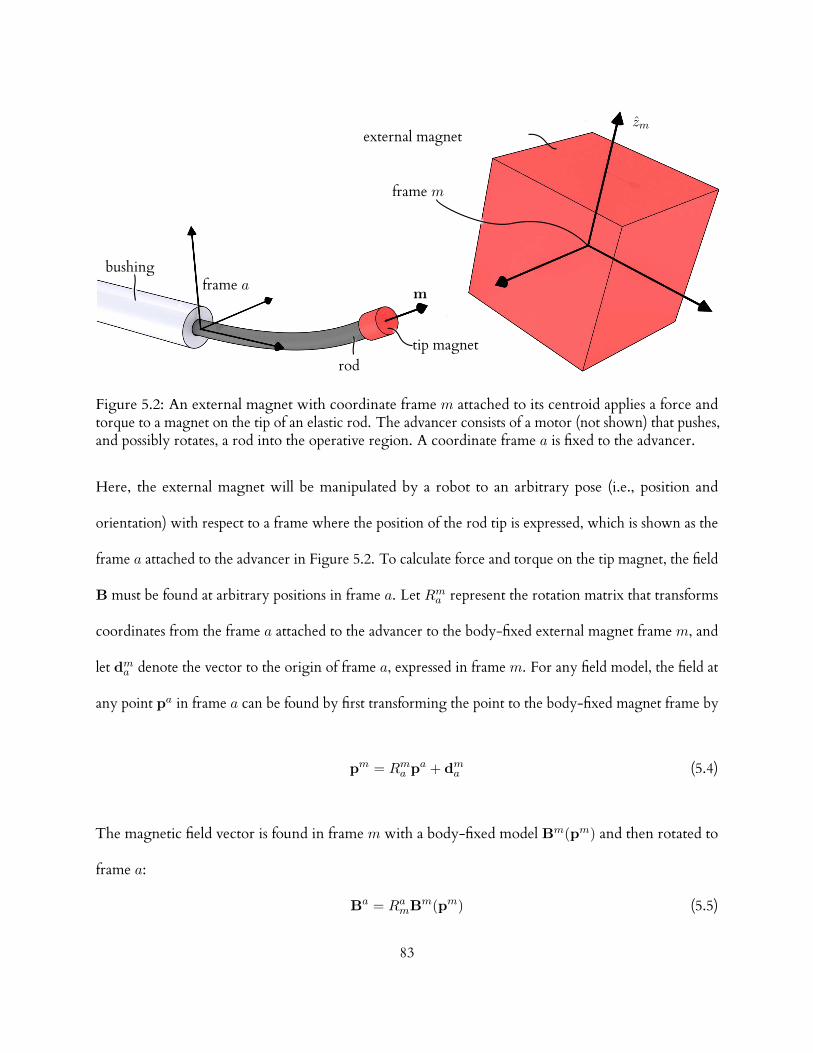
frame a

frame m

tip magnetrod

zmexternal magnet

bushing

m

Figure 5.2: An external magnet with coordinate frame m attached to its centroid applies a force andtorque to a magnet on the tip of an elastic rod. The advancer consists of a motor (not shown) that pushes,and possibly rotates, a rod into the operative region. A coordinate frame a is fixed to the advancer.

Here, the external magnet will be manipulated by a robot to an arbitrary pose (i.e., position and

orientation) with respect to a frame where the position of the rod tip is expressed, which is shown as the

frame a attached to the advancer in Figure 5.2. To calculate force and torque on the tip magnet, the field

B must be found at arbitrary positions in frame a. Let Rma represent the rotation matrix that transforms

coordinates from the frame a attached to the advancer to the body-fixed external magnet frame m, and

let dma denote the vector to the origin of frame a, expressed in frame m. For any field model, the field at

any point pa in frame a can be found by first transforming the point to the body-fixed magnet frame by

pm = Rma pa + dma (5.4)

The magnetic field vector is found in frame m with a body-fixed model Bm(pm) and then rotated to

frame a:

Ba = RamBm(pm) (5.5)

83

5.4 Magnet-Tipped Rod Model

We use the Kirchho rod model [145–149] to solve for large, three-dimensional deflections of a magnet-

tipped rod. This model represents a thin rod as a one-dimensional curve that can bend and twist under

load, but is assumed to be inextensible and unshearable2. The static Kirchho rod problem culminates

in a set of ordinary dierential equations, which we will treat as a two-point boundary value problem

(BVP). Our review of Kirchho’s rod theory in this section is inspired by [150].

5.4.1 Kinematics

The centerline of an undeflected rod is represented by an arc-length parameterized space curve p(s) ∈ R3,

expressed in some fixed frame. An orthonormal frame is attached to each point on p(s), and is represented

by a rotation matrix R(s), where the tilde symbol denotes association with the undeflected curve. Each

local coordinate frame represents the orientation of rod material at the point where it is attached. Under

load, p(s) deflects to a curve p(s), and the R(s) rotate to R(s), in general. Figure 5.3 illustrates the

deflection of a rod and the ensuing rotations of a few local frames.

We assign frames on the undeflected curve such that the z-axis of each frame is tangent to the

curve. Frames constrained in this way are called adapted frames. An arc-length parameterized curve

has a tangent vector of unit length [151, Ch. 2]. Using a prime symbol to denote dierentiation with

respect to s, the adapted frame constraint can be written as

p′(s) = R(s)ez (5.6)

in which ez =

[0 0 1

]T.

2These are reasonable assumptions provided that the rod is neither bent into sharp corners nor subjected to extreme lateralloads [149, Ch. 3, Sec. 7].

84

p(s)

p(s)

Figure 5.3: A rod is modeled in Kirchho’s theory as a space curve with a local coordinate frame attachedto each point. A few frames are shown at corresponding positions on an undeflected curve p(s) (whichmay be arbitrarily precurved), and on the deflected curve p(s) of the same rod.

The angle of rotation of each frame about a rod’s centerline is not constrained by Equation 5.6,

and must be chosen in some way. If the rod is initially straight and has a radially symmetric cross-section,

choosing all R(s) as identity matrices aligns them to the fixed frame. If the rod is precurved and has

asymmetric cross-sections, the x and y axes of each frame can be aligned to the principle axes of each

cross-section. If the rod is precurved and radially symmetric, any of several curve framing methods

based on the dierential geometry of the centerline can be used to assign adapted frames, such as the

Frenet-Serret formulas [151, Ch. 2] or the parallel transport method [152, Ch. 20], [153].

5.4.2 Constitutive Relations

The derivative of R(s) with respect to arc-length can be expressed as

R′(s) = R(s)U(s) (5.7)

85

in which U is a skew-symmetric matrix. Omitting the argument s for brevity,

U =

0 −uz uy

uz 0 −ux

−uy ux 0

(5.8)

The elements ux, uy, and uz can be seen as components of an axial vector u. Curvatures about the x and

y axes are given by ux and uy, respectively, and the torsional twist rate is denoted by uz. A vector u

is found in a similar fashion from R(s). Vectors can also be mapped to skew-symmetric matrices, an

operation we will denote by [·]×.

The vector ∆u(s) = u(s)− u(s) gives the strain at each material point s. The bending strains

about the local x and y axes are given by ∆ux(s) and ∆uy(s), respectively, and the torsional strain is

given by ∆uz(s).

We will assume that the rod material is linear-elastic and denote the elastic modulus function

by E(s) and the shear modulus function by G(s). The second moments of area about the principle

axes of the rod cross-section are denoted by Ix(s) and Iy(s). The polar moment of inertia about the

rod centerline, Jz(s), is found by Jz(s) = Ix(s) + Iy(s). Omitting the argument s for brevity, these

variables can be arranged into a stiness matrix

K =

EIx 0 0

0 EIy 0

0 0 GJz

(5.9)

The internal moment at any point is proportional to the internal strains. This constitutive

86

relationship can be written as

τ = RK∆u (5.10)

It will be useful to rearrange the above equation in the form

u = K−1RTτ + u (5.11)

5.4.3 Equilibrium Equations

f(σ)

l(σ)

−n(s)

−τ (s)

n(L)

τ (L)

Figure 5.4: Equilibrium equations are found by cutting the rod at an arbitrary point p(s) and summingall loads from this point to the rod tip. All loads act on the rod’s centerline, and include an internal forceand torque at s (n(s), τ (s)), distributed forces and torques along the segment (f(σ), l(σ)), and a forceand torque at the tip (n(L), τ (L)).

We show the forces and torques acting on an isolated segment of a rod in Figure 5.4. The

segment extends from an arbitrary point p(s) to the tip p(L). The internal force n(s) and internal

torque τ (s) act in a positive sense across the cut on the portion of rod that extends from the base of the

rod to s.

Distributed forces and torques that act along the rod are denoted by f(σ) and l(σ) respectively,

where σ is a dummy variable for integration. Such loads could be caused by tissue in contact with the

87

rod, for example. The sum of forces on the cut segment of rod is

−n(s) +

∫ L

sf(σ) dσ + n(L) = 0 (5.12)

The total moment on the segment, taken about the origin of the fixed frame, includes the

internal torque at p(s), the moment of the internal force at p(s), the integral of the distributed torque,

the integral of the moment of the distributed forces, the tip torque, and the moment of the tip force:

−τ (s)− p(s)× n(s) +

∫ L

s[l(σ) + p(σ)× f(σ)] dσ

+τ (L) + p(L)× n(L) = 0

(5.13)

Equilibrium dierential equations are found by dierentiating Equations 5.12 and 5.13 with

respect to s to obtain

n′(s) + f(s) = 0 (5.14)

τ ′(s) + p′(s)× n(s) + l(s) = 0 (5.15)

5.4.4 Boundary Conditions

Up to this point we have presented a general Kirchho rod model. Here, we will describe boundary

conditions through which the advancer and robot enter the model. We will specify boundary conditions

for a rod with and without a protective bushing, shown schematically in Figures 5.5 and 5.6. In both

configurations, a rigid post connects the base of the rod to actuators inside the advancer, which are not

shown.

The bushing is useful as a rigid conduit to guide a rod to an operative region. A fixed frame,

88

labelled a in Figure 5.5, is placed at the distal end of the bushing, oriented such that its z-axis is aligned

with the bushing’s centerline. The advancer translates the rod by a distance `(t) along the z-axis and

rotates it by an angle ψ(t) about the same axis (such rotation may be useful with a precurved rod, or if

the tip magnet axis is not aligned with the rod centerline). The time t is held constant when solving the

BVP and will be omitted as an argument in the remainder of this subsection. We will view the advancer

and robot joints as functions of time in Section 5.5, where the rod’s motion is planned as a succession of

equilibrium states.

ψ(t)

s = sas = L

`(t)

L

a

R(0)

post

bushing

Figure 5.5: A bushing, shown in section view, guides the rod to the operative region. The base of therod is actuated via a rigid post which translates the rod by a distance `(t) and rotates it by an angle ψ(t)relative to frame a. A two point boundary value problem is solved with endpoints at sa and L.

The material point that coincides with the origin of frame a is denoted by sa = L−`, whereL is

the total length of the rod. We will solve the BVP over the interval [sa, L], which spans the unconstrained

part of the rod.

If the rod is radially symmetric, it may twist within the bushing. We assume that the bushing

is frictionless and therefore cannot apply torque about the rod centerline. If the rod is precurved, the

bushing exerts reaction forces to conform the rod to the bushing’s centerline, but these transverse

forces cannot cause torsional deformation because the shear center of a Kirchho rod coincides with its

89

centerline [154]. Thus, deformation in the bushing consists solely of twisting around the local z-axis,

and is caused exclusively by τz(sa), the z-component of the internal moment at the distal end of the

bushing. The z-axes of the local frames are aligned within the bushing, thus the transposed rotation

matrix in Equation 5.11 does not aect the z-component of u(s), which becomes

uz(s) =τz(sa)

G(s)Jz(s)+ uz(s) (5.16)

The bushing constrains the position and direction of the rod centerline at p(sa), but the frame R(sa) is

rotated about the z-axis by an angle

φ = ψ +

∫ sa

0uz(s) ds (5.17)

Thus, the boundary conditions at sa are

p(sa) = 0 (5.18)

R(sa) = Rz(φ)

(5.19)

where Rz(·) is a rotation about the fixed z-axis. Note that the angle φ depends on the constant τz(sa),

which is unknown at the outset of solving the BVP. In the next subsection we will discuss methods for

finding τz(sa) and other unknown constants using a numerical BVP solver.

If a non-radially symmetric rod is used, a bushing may be designed to prevent the rod from

twisting or rotating (e.g., a “D”-shaped rod in a similarly shaped hole). For such a bushing, rotation by ψ

could be implemented as rotation of the entire bushing about the fixed z-axis, whereby conditions 5.18

and 5.19 can be applied by setting φ = ψ.

90

ψ(t)

s = 0 s = L

a

`(t)

L

a0

post

Figure 5.6: The bushing may be discarded to accommodate tapered or other unusual rod shapes. In thiscase, the BVP is solved over the fixed interval [0, L], and the advancer displacements `(t) and ψ(t) areinterpreted as parameters of a rigid transformation of frame a with respect to an initial pose a0.

The pose of the external magnet (frame m) is known, in general, with respect to the robot

base frame r from a forward kinematic function in the form

T rm = T rm (θ) (5.20)

in which T is a 4×4 homogeneous transformation matrix, and θ is a joint displacement vector. We assume

that the pose of the advancer frame a is known relative to the robot base frame r as a transformation T ra .

For a particular robot posture, the field B at position p(L) is found using Equations 5.4 and 5.5, obtaining

Rma and dma from Tma = Tmr Tra . The tip position p(L) depends on the equilibrium configuration of the

rod, and like τz(sa), this constant is unknown when beginning to solve the BVP.

It may sometimes be desirable to dispose of the bushing, as shown in Figure 5.6. This configu-

ration could be useful if the rod is tapered, for example. We embed frame a in the base of the rod in

this case, and interpret ` and ψ as displacements of frame a relative to the pose a0 at which T ra has been

91

measured. Thus, the pose of the advancer relative to the magnet now becomes

Tma = Tmr Tra

Rz(ψ) `ez

0 1

(5.21)

By setting sa = 0, boundary conditions 5.18 and 5.19 hold as stated above.

Next, we consider loads on the tip. The tip magnet may be attached in any orientation with

respect to the tip frame R(L), though it may often be convenient to align its magnetization vector with

the rod centerline. Let the unit vector d in frame R(L) denote the direction of the magnetization vector

with respect to the rod tip. The magnetization vector m can be factored as ‖m‖ m, where ‖m‖ may be

approximated as suggested in Section 5.3, and m is a unit vector expressed in the fixed frame as

m = R(L) d (5.22)

The vector m depends on the equilibrium tip frame orientation R(L), and is thus an additional unknown.

The force and torque exerted by the external magnet on the tip magnet are found using

Equations 5.2 and 5.3. We add a gravitational force G to prescribe the conditions

n(L) = (m · ∇) B + G (5.23)

τ (L) = m×B (5.24)

5.4.5 Numerical Solutions

Analytic solutions have been found for a few special Kirchho rod problems, but solutions for three-

dimensional deflection problems usually require numerical methods, such as the finite-dierence or

92

finite-element methods.

The magnet-tipped rod BVP is given by Equations 5.6, 5.7, 5.14, and 5.15, together with the

boundary conditions stated in Equations 5.18, 5.19, 5.23 and 5.24.

We use the bvp5c function in Matlab (The Mathworks, Natick, MA) by Kierzenka and

Shampine [155] to solve the BVP. This solver implements a finite-dierence method based on the

four-stage Lobatto IIIA collocation formula, and can find unknown parameters that appear in a BVP.

We use this capability to find the parameters

Π =

τz(sa)

p(L)

m

(5.25)

Many BVP solvers are not explicitly designed to solve for unknown constant parameters.

However, by augmenting the state equations with the trivial equations

Π′ = 0 (5.26)

any BVP solver can be used to solve the problem (see [156, Ch. 1]). Additional boundary conditions

follow from the definition of Π. For example, Π1(sa) = τz(sa), Π2(L) = px(L), etc.

Without a good initial guess, BVP solvers often fail to find a correct solution, or potentially

any solution at all. In the next section we will describe a method to incrementally displace a rod to follow

a trajectory, in which a solution obtained at step n furnishes a guess for the solution sought at step n+ 1.

The bvp5c solver returns and accepts a set of data that includes optimal collocation mesh points, the state

variables at those points, and the parameter values found at the end of an iteration. We pass all of this

93

data forward to the subsequent iteration as an initial guess.

5.5 Trajectory Following

5.5.1 Forward Kinematics

Each solution of the magnet-tipped rod BVP describes the full, deflected shape of the rod. To plan

trajectories, we limit our attention to the rod tip, and introduce the variable r(t) to represent the tip

position p(L) that is found by solving the BVP with the boundary conditions applied by the advancer

and robot at time t.

We group the advancer and robot joint variables as

q(t) =

ψ(t)

`(t)

θ(t)

(5.27)

Let p denote the advancer degrees of freedom, such that p = 1 if only `(t) is actuated, and p = 2 if ψ(t)

is also actuated. Thus, if the robot has j joints, then q has dimension p+ j.

With the variable q, the forward kinematics of the cooperative advancer-robot system can be

expressed as a function Ω : Rp+j → R3

r = Ω(q)

(5.28)

We wish to invert Ω to find a joint trajectory q(t) corresponding to some desired tip trajectory

r(t). However, Ω is not amenable to direct inversion because q may not be unique and Ω is found as a

solution of a dierential equation. We will find solutions to the inverse problem that use the Jacobian

matrix J ∈ R3×(p+j) of Ω. Using a raised dot symbol to denote dierentiation with respect to time, the

94

Jacobian J maps the control vector velocity q to the tip velocity r

J(q) =∂Ω(q)

∂q(5.29)

r = J(q) q (5.30)

5.5.2 Inversion and Redundancy Resolution

If J is square and full rank, then it can be inverted to solve for a unique q. If either p = 1 and j > 2 or if

p = 2 and j > 1, then the system is redundant to the tip control task, provided that J is full (row) rank.

The advancer and robot form a cooperative system in which the rod tip position is the output, and the

robot end-eector is analogous to an intermediate link in a more traditional robot structure. There are,

in general, multiple solutions for the external magnet pose. The Jacobian that maps the spatial velocity of

the external magnet to the force/torque wrench on the tip magnet is rank five for dipole magnets [104]

(rotations about the dipole axis leave the field unchanged). Thus, perturbations of the external magnet

pose alter the tip boundary conditions and change the shape of the rod.

Redundancy may be exploited to fulfill secondary goals. We will solve for q in the redundant

case using weighted generalized inverses [157] of the Jacobian, denoted by J#. A weighted norm of

joint rates is given by

‖q‖W =(qTW q

) 12 (5.31)

in whichW ∈ R(p+j)×(p+j) is a positive-definite weighting matrix. A vector q that minimizes Equa-

tion 5.31 and satisfies r = J q can be found by minimizing the cost function C

C(q, λ) =(qTW q

) 12

+ λT(r− J q) (5.32)

95

where λ is a vector of Lagrange multipliers. If J is full (row) rank, the weighted least norm solution to

Equation 5.32 for q is

q = W−1JT(JW−1JT

)−1r (5.33)

The productW−1JT(JW−1JT

)−1 will hence be denoted by J#.

A robot’s joints may include a combination of prismatic and revolute types, and may have

dierent joint limits, torque limits, etc. The matrixW can be chosen to emphasize the contribution of

certain joints to a weighted least norm solution. If the joint weight matrixW is diagonal, each entry

wi along the main diagonal independently weights one joint axis. Increasing a weight wi decreases the

contribution of the corresponding joint. If all joints are equally weighted (W = I), then J# reduces

to the Moore-Penrose pseudoinverse. We will denote an initial matrix of joint weights chosen for the

above considerations byW0, to distinguish it from a final matrixW , which we will describe shortly.

Joint weights can be varied during robot motion to fulfill secondary tasks with a redundant

robot. Chan and Dubey [158] employed a penalty function that increased as joints approached their

limits. Joint weights were calculated from the gradient of this function to push joints away from their

limits. Park et al. [159] and Xiang et al. [160] both presented formulations based on the weighted

generalized inverse for fulfilling multiple subtasks with a redundant robot.

5.5.3 Avoiding an Obstacle Using a Virtual Wall

Wewill adjustW to deflect the external magnet away from a virtual wall established between the external

magnet and the patient or other forbidden region, such as that surrounding a surgical instrument. We

represent the wall by an infinite plane, parameterized by a unit normal vector n pointed away from

the prohibited side of the wall, and by the shortest distance of the wall from the origin of the reference

frame, denoted by D. The position of the centroid of the external magnet in frame a is found using

96

Equation 5.20 and is denoted here by x. The shortest distance d from the center of the external magnet

to the plane is given by

d = n · x +D (5.34)

A function H is chosen to increase rapidly as the external magnet approaches the wall. We

adapt the following artificial potential field function from Khatib [161]

H (d) =

η(

1d −

1ε

)2, if d ≤ ε

0, if d > ε

(5.35)

The constant gain factor η scales the magnitude of H , and ε is an activation threshold distance.

Let v be a combination of the linear velocity of the advancer ˙, the angular (roll) velocity of

the rod ψ, the translational components of the robot end-eector velocity x, and the angular velocity

vector of the external magnet ω as

v =

ψ

˙

x

ω

(5.36)

The Jacobian of the advancer is a trivial identity matrix, because ˙ = dq1dt and ψ = dq2

dt . Using the robot’s

geometric Jacobian Jr, a combined advancer-robot Jacobian Jar can be expressed as

Jar =

Ip 0

0 Jr

(5.37)

97

such that

v = Jarq (5.38)

Whitney [162] observed that a weighted norm can be defined for the spatial velocity of a redundant

robot’s end-eector and then transformed into a corresponding joint norm. A positive-definite weighting

matrix W of dimension n×n, in which n are the degrees of freedom of the robot end-eector, establishes

the norm

‖v‖W =(vTWv

) 12 (5.39)

Substituting Equation 5.38 into Equation 5.39 yields

‖v‖W =(qTJT

arWJarq) 1

2 (5.40)

By comparing Equations 5.31 and 5.40, it is seen that W is obtainable from W by a congruence

transformation

W = JTarWJar (5.41)

in which it is assumed that Jar is nonsingular. We will choose W to be a diagonal matrix and, numbering

diagonal elements from the upper left corner, we will increase the elements wp+1 through wp+3 to

suppress corresponding components of x as the external magnet approaches the wall. Depending on the

direction of x, some of its components xi may cause H to increase at a faster rate than others and should

be attenuated proportionally. Inspired by [158], we will use the absolute values of the components of

∇H to weight the components of W corresponding to x.

The weighted Jacobian solution does not distinguish among the directions of the weighted

variables. No weighting should be used for components of x headed away from the wall, otherwise the

98

external magnet will tend to become “trapped” near the wall. The wall normal vector has components

n =

[n1 n2 n3

]T. If any component of x is directed away from the wall, its corresponding weight

wi is set to zero.

wp+i =

∣∣∂H(d)∂xi

∣∣, if xini ≤ 0

0, if xini > 0

(5.42)

The joint weights required for Equation 5.33 are then found by

W = W0 + JTarWJar (5.43)

Alternatively, an initial weight matrix W0 can be specified in the robot’s task space, perhaps using an

inertia tensor or other application-specific weighting. With this method, the joint weights are given by

W = JTar

(W0 + W

)Jar (5.44)

5.6 Experimental Methods

We assembled a magnet-tipped rod guidance system to execute experimental trajectories while measuring

the rod tip positions. The experimental apparatus was arranged on a benchtop as illustrated in Figure 5.7.

5.6.1 Advancer and Magnet-Tipped Rod

The rod was a straight, glass optical fiber (Item 57 062, Edmund Optics, NY, USA), 10 cm in length

with a diameter of 0.24 mm. Two NdFeB magnets (Cyl-0010, Engineered Concepts, Birmingham, AL,

USA) were attached coaxially to the tip of the rod using cyanoacrylate adhesive (Loctite 4014 Prism

Instant Adhesive, Henkel Corp., Rocky Hill, CT, USA). The magnets were cylinders, each 0.75 mm in

diameter and 1 mm long. Each magnet was grade N50, and was magnetized along its cylindrical axis.

99

robot

advancer

external magnet

rod

stereo cameras

benchtop

Figure 5.7: Experimental apparatus. A NdFeBmagnet was mounted to a six-degree-of-freedom (6-DOF)serial robot to guide a magnet-tipped rod along trajectories. The length of rod was varied by a 1-DOFadvancer. A stereo-camera pair was used to measure rod tip positions. The cameras were not used forfeedback.

The advancer, shown in Figure 5.8, consisted of a rigid acrylic frame that housed a piezoelectric

linear motor (SLC-1770, SmarAct GmbH, Oldenburg, Germany) which had an encoder resolution of

1 µm. The rod was attached to a vee-shaped clamp on the moving slide of the motor. This clamp applied

the boundary conditions stated in Equations 5.18 and 5.19, with ψ = 0, as we did not rotate the rod. A

low-friction bushing on the top surface of the acrylic was fabricated from a 3.2 mm thick sheet of acetal

polymer using a CO2 laser cutting machine.

5.6.2 Robot and External Magnet

A six-degree-of-freedom serial robot (Model RV-3S, Mitsubishi Electric US, Inc., Cypress, California)

was used to manipulate the external magnet. The position repeatability of the robot was 0.02 mm,

according to the manufacturer.

100

advancer

rod

external magnet

robot

tip magnet

bushing

(b)(a)

a

motor

Figure 5.8: (a) A cube-shaped NdFeB magnet was held in a fixture attached to the robot. (b) The rodwas an optical fiber, 0.24 mm in diameter, which had two small NdFeB magnets attached to its tip. Therod was pushed by a linear motor through a bushing that constrained the position and direction of therod.

The external magnet was a cube-shaped, grade N52 NdFeB magnet (NB064-N52, Applied

Magnets, Plano, TX, USA), with an edge length of 5.08 cm. The magnet was placed in a fixture attached

to the robot end-eector, which is shown in Figure 5.8. The magnet was oriented in the fixture with its

magnetization vector orthogonal to the robot’s sixth joint axis.

In order to position the external magnet to desired poses with respect to the advancer frame

(frame a in Figure 5.5 or frame a0 in Figure 5.6), a registration procedure was required to determine the

pose of the robot’s base frame with respect to the advancer frame. The relationship between these frames

101

is described by transformation T ra in Section 5.5, and could be obtained in many ways. For example,

in a clinical setting, one might attach optically tracked markers to both the robot and the advancer, to

continuously observe the position of each in a common reference frame. In our benchtop experiments,

neither the advancer nor robot base frame moved, so it was not necessary to continuously track their

positions (T ra was constant). Thus, we obtained transformation T ra by placing the robot’s end-eector

at a known pose with respect to the advancer by fitting a feature on the external magnet fixture to a

matching feature on the advancer housing.

5.6.3 Trajectory Computation and Control

We planned trajectories by numerically integrating Equation 5.33 using Matlab software. A central

dierence formula was used to approximate the Jacobian. The notation [J(q)]•,n signifies all rows of the

nth column of J , which were obtained by

[J(q)]•,n ≈Ω(q + hn)− Ω(q− hn)

2h(5.45)

in which h ∈ R is a small increment and hn ∈ Rp+j is a vector with h in the nth row and zeros in all

other rows. Small errors caused by discretization of the rate variables and numerical approximation of

the Jacobian tend to accumulate during numerical integration. We found that drift is eectively reduced

by a closed-loop inverse kinematics (CLIK) algorithm [163] of the form

q = J# (q) r + Γ (r− Ω(q)) (5.46)

in which the scalar Γ < 1 is a closed-loop gain constant.

We wrote a program in the C language to control the serial robot and advancer, and to trigger

102

acquisition of stereo images. The program executed pre-planned trajectories on a desktop computer

with a 2.67 GHz Intel Xeon processor, which ran a Linux Ubuntu 11.04 operating system.

5.6.4 Stereo Camera Measurements

Two digital cameras (XCD-X710, Sony Corporation, Japan) were mounted in a stereo configuration

to a rigid aluminum frame attached to the benchtop, approximately 40 cm from the advancer. Prior to

acquiring experimental images, we used the OpenCV library [164] to find stereo calibration parameters

from images of a checkerboard pattern. During trajectory execution, the control software automatically

triggered acquisition of image pairs. Each image measured 1024 × 768 pixels, and was processed to

correct lens distortion using the OpenCV library.

Tomeasure a three-dimensional point, image coordinates of the point were manually selected in

corresponding images. The three-dimensional point was then triangulated using an iterative least-squares

method that minimized the stereo reprojection error [165].

It was necessary to transform measured points, which were found in the camera frame c, to the

advancer frame a for comparison with planned trajectory points. To find the origin of frame a relative

to c, we measured the position of the advancer hole. The advancer frame was defined to be parallel to the

robot base frame r. An optical target was attached to the robot end-eector and translated along each

coordinate direction of frame r, and the endpoints of these translations were measured to find the axes

of frame r within frame c. With the position and orientation of frame a relative to c, we constructed a

transformation T ac to transform measured points to frame a.

5.6.5 Calibration

We calibrated our model by adjusting the small set of sensitive parameters listed in Table 5.1. Parameter

EIx is the bending stiness of the rod. The rod had a circular cross-section, therefore EIy = EIx. The

103

torsional stiness GJz was calculated to be 5.33× 10−6 N m2 from the calibrated value of EIx. The

magnetizations of the external magnet Mext and tip magnet Mtip have a large eect on accuracy because

the calculated forces and torques on the tip magnet depend on the magnitudes of these two quantities.

The mass of the tip magnet mtip determines the gravitational force G in Equation 5.23. The total

rod length L was initially measured to be 10 cm, but the process of manually clamping the rod to the

motor caused some uncertainty in this parameter. Parameters δx, δy, and δz are small corrections to

the translational components of T ra . Rotational components of T ra were excluded because frame a was

defined to be parallel to r in the registration process described above, and enabling rotation between

these frames did not significantly improve calibration results during initial sensitivity tests.

A set of 60 randomized q vectors were used for parameter calibration. They prescribed poses

for the robot and advancer at which images were acquired with the stereo cameras. The kth rod tip

position as measured from the stereo images is denoted by rk. The kth rod tip position found by solving

the BVP with controls qk and parameter vector γ is denoted by Ω(qk,γ). An initial guess for γ was

selected by coarse adjustment of nominal values. We used the fmincon function in Matlab to find the

parameters γcal that minimize the objective function

γcal = arg minγ

(60∑k=1

‖rk − Ω(qk;γ)‖

)(5.47)

This function computes the error between predicted and measured tip positions, summed over the

calibration set. We define tip error as the Euclidean norm of the dierence between a measured tip

position and a modeled tip position. After finding optimal calibration parameters, the mean tip error for

the calibration set was 0.62 mm.

104

Table 5.1: Calibrated values of model parameters

Parameter Value

EIx 6.17× 10−6 N m2

‖Mext‖ 1.21× 106 A/m

‖Mtip‖ 1.24× 106 A/m

mtip 3.65× 10−5 kg

L 98.75 mm

δx 2.00 mm

δy 0.43 mm

δz 1× 10−5 mm

5.7 Experiments

We executed several three-dimensional, open-loop rod tip trajectories planned using the methods

described in Section 5.5. The mean and standard deviation (SD) of tip error measurements for each

trajectory are presented in Table 5.2, which also lists the number n of tip measurements for each trajectory.

Advancer frame coordinate axes are shown in each figure below, where the positive x-axis points toward

the midpoint of the stereo cameras. With the exception of the trefoil knot trajectory discussed below,

we planned trajectories using all six joints of the robot. The pseudoinverse of J was used to plan all

trajectories except the virtual wall trajectory, in which a weighted generalized inverse was used.

Table 5.2: Rod tip error

Trajectory Mean (mm) SD (mm) n

Square, xy plane 0.98 0.22 199Square, zx plane 0.83 0.07 199Square, zy plane 0.96 0.25 199Concho-spiral 1.02 0.32 249Square, xy plane with obstacle 1.07 0.23 249Trefoil knot, 2-DOF robot 1.52 0.48 249

Figure 5.9(a) shows tip measurements from three square-shaped tip trajectories within mutually

orthogonal planes. This experiment tested the ability to track straight lines in various positions and

105

orientations. Each square had a planned edge length of 2 cm, and was executed with a tip velocity of

0.4 mm/s. The center of each square was located 6 cm above the origin of the advancer frame. The

full rod shape found by solving the BVP (i.e., the planned shape) is shown at the starting point of each

trajectory. A composite photograph of 40 sampled positions from a video recording of the zy-plane

trajectory is shown in Figure 5.9(b).

x (mm)y (mm)

z(m

m)

-100

10 -100

100

10

20

30

40

50

60

70

rod solutions

measured points

(a) (b)

Figure 5.9: (a) The tip of the rod was guided along three square-shaped trajectories, each with an edgelength of 2 cm. Measured tip positions are shown as dots, with the planned trajectories shown as solidlines next to the dots. Examples of rod solutions are shown at the starting point of each trajectory. (b)Composite photograph constructed from 40 sampled positions of the zy-plane square trajectory.

We next tested a curved trajectory, the concho-spiral, shown in Figure 5.10. The concho-spiral

is a logarithmic spiral wound around a cone, with a curvature inversely proportional to arc-length [166].

106

This trajectory tested tip accuracy for both small rod deflections (toward the apex of the cone), and large

deflections (toward the base). The trajectory is given in cylindrical coordinates by

r = β ϕµη (5.48)

θ = β η (5.49)

z = z0 + β ξ µη (5.50)

We solved for parameter η to plan a constant tip speed of 0.4 mm/s. Parameters µ, ϕ, and ξ control the

spiral’s shape, which we chose as 1.04, 0.08, 0.05, respectively. The scaling factor β = 0.0167 was chosen

to fit the shape into the rod tip workspace. The oset distance z0 is places the apex of the spiral 6 cm

above the origin of the advancer frame.

x (mm)y (mm)

z(m

m)

-150

15

-150

15

65

75

85

Figure 5.10: The concho-spiral trajectory tested accuracy over a range of rod deflections.

To test obstacle avoidance, we projected a virtual planar wall into the workspace of the external

magnet. The planned tip trajectory was a square in the xy plane of frame a, identical to that shown in

Figure 5.9, but now starting from the center of the square and following a diagonal line toward the first

107

corner. An initial weighting matrix W0 = I6 was used with Equation 5.43, as this was found to result

in smooth motion of the external magnet. Figure 5.11 shows both the rod tip measurements and the

planned motion of the external magnet centroid, which begins by tracking the diagonal line of the rod

tip but is deflected by the virtual wall. An external magnet trajectory planned without wall avoidance is

also shown as a dashed line, and violates the wall (the rod tip measurements for this unweighted external

magnet trajectory are those shown in Figure 5.9).

x (mm)

y (mm)

z(m

m)

-200

20-20

0

20

80

100

120

140(a)

(c)

(b)

(e)

(d)

Figure 5.11: The external magnet trajectory (a) violates a virtual wall (b) when used to guide the rod tipalong a square trajectory. By using an artificial potential function emanating from the wall to adjust aweighted Jacobian, the external magnet instead moved along trajectory (c). The measured tip positions(d) are shown for external magnet trajectory (c), with the planned trajectory shown as a solid line (e).

Although we believe that it will be useful to build some redundancy into a magnetic steering

system like the one we describe in this paper, inspection of Equation 5.28 suggests that a simple, two-

108

degree-of-freedom robot can be used to manipulate the external magnet (the advancer provides a third

DOF when enabled to translate). For example, the external magnet could be translated within a plane,

or gimbaled to rotate about two orthogonal axes.

To explore this, we planned a trajectory for a 2-DOF virtual robot restricted to translate the

external magnet in a plane parallel to the xy-plane of the advancer frame, at a height of 12 cm above the

origin of the advancer frame. The trajectory was a trefoil knot space curve, given by the parametric

equations

x = β[sin(t) + 2 sin(2t)]

y = β[cos(t)− 2 cos(2t)] (5.51)

z = z0 − β sin(3t)

in which t ranged from 0 to 205 seconds, β = 5× 10−3, and z0 = 6 cm. The 2-DOF trajectory of the

virtual robot was executed with our 6-DOF robot by solving the inverse kinematics of the 6-DOF robot

for the planar external magnet trajectory. Both rod tip position measurements and the planned motion

of the external magnet are shown in Figure 5.12.

5.8 Conclusion

Complex, three-dimensional tip trajectories of magnet-tipped rods are attainable by robotically manipu-

lating a permanent magnet. Our approach combined the kinematics of the robot and advancer with a

Kirchho rod model and a magnetic field model. We linearized the overall system model by computing

its Jacobian, and demonstrated accurate trajectory following and obstacle avoidance using resolved-rate

motion control.

Our experimental results suggest that open-loop trajectory following may provide sucient

109

x (mm) y (mm)

z(m

m)

-30-15

015

30 -30

-15

0

15

30

60

80

100

120

(a)

(b)

Figure 5.12: (a) To simulate a 2-DOF robot, the external magnet trajectory was restricted to translationswithin a plane. (b) The rod tip was guided along a trefoil knot trajectory, a three-dimensional spacecurve.

accuracy for clinical applications, though further analysis is necessary to establish accuracy requirements

for specific procedures. Medical imaging, such as fluoroscopy or computed tomography (CT), could

provide tip position feedback to improve accuracy using a closed-loop control scheme.

110

CHAPTER 6

CONCLUSIONS

This dissertation contributed methods, experimental results, and analysis to improve mini-

mally invasive electrode implantation. In this section, we consider the implications of our results, and

recommend directions for future work.

6.1 Improvements to Stereotactic Surgery Using Robots

Adjustment of a stereotactic device is a well-defined mechanical task that is suited to automation. The

task entails transfer of measurements from software to a physical device, and in this sense resembles many

other repetitive industrial tasks for which robots have supplanted human operators, with benefits to the

cost, safety, and time required for manufacturing. To realize similar benefits in the operating room, we

designed robotic stereotactic systems for the surgical workflows of minimally invasive cochlear implan-

tation surgery and deep brain stimulation surgery. In particular, we designed systems for compatibility

with existing trajectory planners and for the special implantation tools used in each surgery.

Prior to our work, miniature stereotactic devices were robotically manufactured by 3D printing

and CNC milling. Our designs shifted the robotic task from additive or subtractive manufacturing to

automated adjustment-and-locking of a kinematic structure. Both approaches result in what is essentially a

custom-shaped structure, but automated adjustment-and-locking requires less time and equipment than

manufacturing from bulk material.

In previous applications of robots to stereotactic surgery, the problem of relative motion

between the robot and patient was solved by either actively repositioning the robot to compensate for

patient motion or by securing the patient and robot to a common structure. We attach pre-adjusted

111

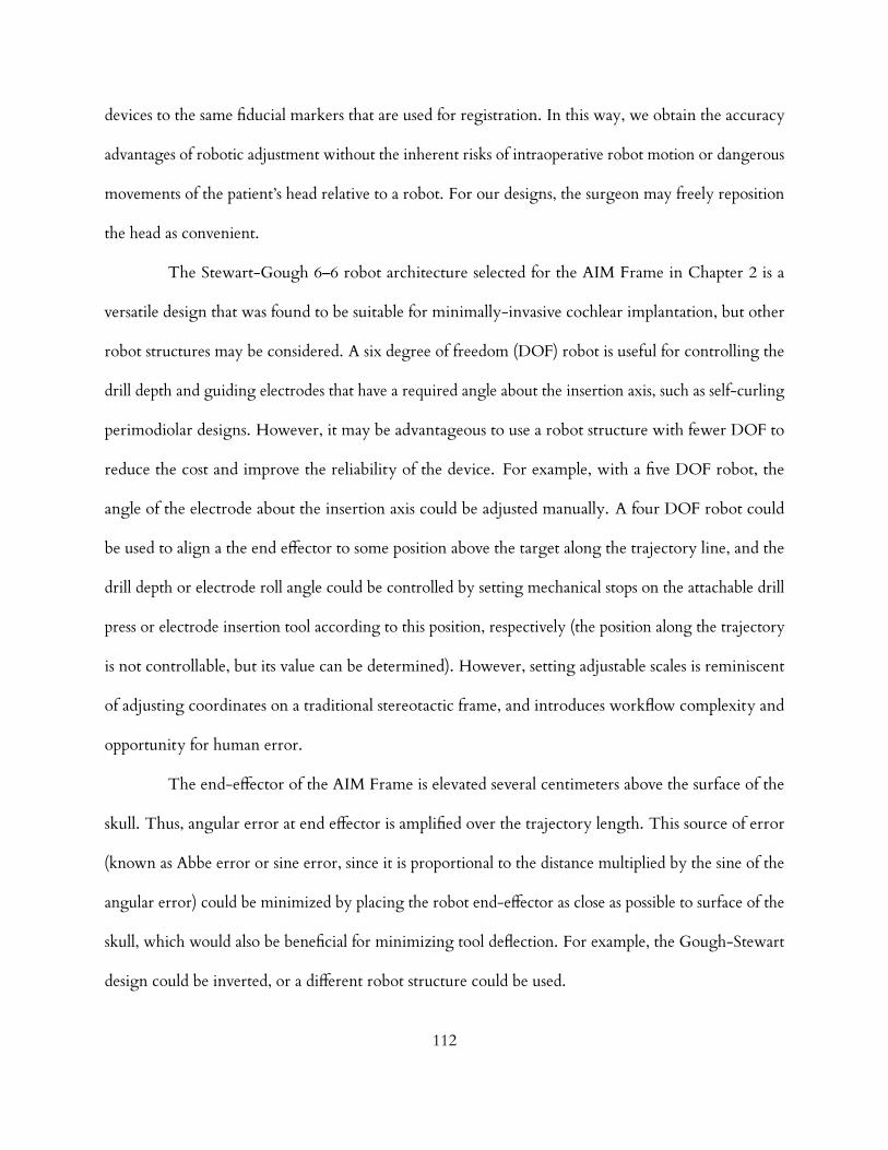
devices to the same fiducial markers that are used for registration. In this way, we obtain the accuracy

advantages of robotic adjustment without the inherent risks of intraoperative robot motion or dangerous

movements of the patient’s head relative to a robot. For our designs, the surgeon may freely reposition

the head as convenient.

The Stewart-Gough 6–6 robot architecture selected for the AIM Frame in Chapter 2 is a

versatile design that was found to be suitable for minimally-invasive cochlear implantation, but other

robot structures may be considered. A six degree of freedom (DOF) robot is useful for controlling the

drill depth and guiding electrodes that have a required angle about the insertion axis, such as self-curling

perimodiolar designs. However, it may be advantageous to use a robot structure with fewer DOF to

reduce the cost and improve the reliability of the device. For example, with a five DOF robot, the

angle of the electrode about the insertion axis could be adjusted manually. A four DOF robot could

be used to align a the end eector to some position above the target along the trajectory line, and the

drill depth or electrode roll angle could be controlled by setting mechanical stops on the attachable drill

press or electrode insertion tool according to this position, respectively (the position along the trajectory

is not controllable, but its value can be determined). However, setting adjustable scales is reminiscent

of adjusting coordinates on a traditional stereotactic frame, and introduces workflow complexity and

opportunity for human error.

The end-eector of the AIM Frame is elevated several centimeters above the surface of the

skull. Thus, angular error at end eector is amplified over the trajectory length. This source of error

(known as Abbe error or sine error, since it is proportional to the distance multiplied by the sine of the

angular error) could be minimized by placing the robot end-eector as close as possible to surface of the

skull, which would also be beneficial for minimizing tool deflection. For example, the Gough-Stewart

design could be inverted, or a dierent robot structure could be used.

112

(a) (b) (c) (d)

Figure 6.1: Miniature Freeze Frame concept, using pre-positioning frame (PPF) (a) Three captive spheressupport sliding rods with spherical tips. The spherical tips lock into gripper mechanisms attached to fixedpositions on the PPF. (b) The spherical rod tips are positioned to calculated points by an external robotto adjust the frame (c) Adhesive injection to lock ball and rod (d) Placement on patient for minimallyinvasive cochlear implantation surgery.

Reducing the size of the Freeze Frame could make it suitable for minimally invasive cochlear

implantation surgery or bilateral deep brain stimulation surgery, which uses a separate trajectory for each

brain hemisphere. The Freeze Frame was designed for attachment to anchors implanted for bilateral

STarFix platforms. The clinical STarFix anchors were spread widely on the top of the head, and there

is considerable variation in these anchor positions with respect to the trajectory, as described in the

Appendix to Chapter 3. The STarFix anchors were used to ground the design in clinical data, but future

iterations of the Freeze Frame concept could be attached to the patient using alternative mechanisms

that facilitate a smaller overall design. For example, the conceptual miniature Freeze Frame shown in

Figure 6.1 attached to a pre-positioning frame (PPF) similiar to that introduced in Chapter 2 for the

AIM Frame. The adjustable “legs” of this device are rods with spherical tips, which slide within captive

spheres that rotate within a platform. The spherical rod tips would be positioned by an external robot

and then locked into radiolucent gripper mechanisms built into the PPF (metal fiducial spheres, not

shown in Figure 6.1, would be embedded in the PPF for registration).

Adhesive locking was proposed for the Freeze Frame because mechanical locking devices,

113

such as the set screws found on a traditional stereotactic frame, are complicated to automate and rely

on forces that may warp a frame. Equipment for automated cyanoacrylate dispensing is widely used in

manufacturing, but assuring that the adhesive flows with clinically adequate reliability into joints of a

Freeze Frame in an arbitrary configuration will be challenging. Several polymer joining methods may

be adaptable to the Freeze Frame concept [167,168], and could be more convenient. For example, in

resistive implant welding [169], a conductive wire or mesh is trapped between two components to be

joined. The conductive element is heated by running a current through it, which causes the parts to bond

with the conductive mesh in place. Such meshes could be manufactured into the Freeze Frame joints.

Other possible methods include laser welding, heated tool welding, and ultrasonic welding. However,

several polymer joining methods create fumes and often require pressure to be applied between parts,

which could distort the frame and reduce its accuracy.

6.2 Force thresholds in CI surgery

As robotic tools for CI insertion become more viable for clinical use, the data to specify the design and

operation of these devices will grow in importance. The mechanical characteristics of intracochlear tissues

are dicult to observe without altering supporting structures. We described a protocol for excising

fresh cochlea and measuring the rupture force of the intact intracochlear partition. Our specimen

preparation method could be extended to test other forms of mechanical trauma, which will be necessary

to characterize the interaction of an electrode with intracochlear structures.

The biomechanics of the cochlea have been extensively studied prior to our work, but with

an aim of understanding sound transduction and disease, rather than the failure analysis that was the

focus of our work. Our empirical results could be given a broader interpretation by relating them to

mechanical models of tissues in the intracochlear partition.

Our results suggest that surgeons can perceive intracochlear rupture forces, but further research

114

is needed to understand perception under the more complicated force loadings than the sudden onset of

force applied by Semmes-Weinstein monofilaments in our experiments. Future experimental designs

could use haptic devices to apply force profiles that closely resemble a full cochlear implant insertion, but

the fatigue of participants should be considered. The staircase testing procedure we described required

approximately 30 minutes per participant, and the surgeons who participated expressed relief at the

conclusion of testing. A portable testing apparatus such as we have introduced will be useful for testing

at a site chosen by participants or at a professional gathering.

6.3 Guiding magnet-tipped electrodes

We described methods for guiding electrodes and other rod-shaped instruments along three-dimensional

trajectories using a robot-mounted external magnet as a field source. Our approach requires considerably

less equipment and energy than the large field sources that are now used clinically to guide magnetic

catheters. Furthermore, we have demonstrated the most accurate, open loop control of a magnet-tipped

rod to date.

One notable advantage of magnet-tipped electrodes is that no mechanical components are

required along the length of the electrode. Thus, existing electrodes can be adapted without modifying

their internal structures; only one magnet needs to be attached to the tip. This aspect facilitates use of

very thin rods, such as the 240 µm diameter optical fiber used in our experiments. Our approach could

be used with considerably thinner rods to perform dexterous procedures in previously inaccessible, small

cavities of the human body.

The Kirchho rod model we described could aid further design and analysis. This versatile

rod model can be extended to include eects such as forces from fluids or contacting tissues, as would

be useful to avoid trauma during electrode implantation, for example. In future work, our model may

serve as a benchmark for low-order rod models which may be suited to real-time planning and control

115

algorithms.

We demonstrated tip guidance using both redundant and non-redundant external robots.

Redundancy may be useful to fulfill several secondary goals. We focused on obstacle avoidance, but

the technique could be expanded to avoid joint limits or singularities of the external robot, for example.

Alternatively, we showed that a minimal, two-degree-of-freedom robot could be used, pointing the

way to range of simple and compact robot designs for manipulating the external magnet. We anticipate

that design choices such as we have noted here will be resolved by particular applications.

The glass optical fiber rod we used in experiments was chosen for its homogeneous material

properties and constant second moment of area. A constant second moment of area made the rod easy to

calibrate. Similar rods could be used for many magnetic guidance applications, such as biopsy needles or

steerable endoscopes. It will be more challenging to calibrate existing devices such as cochlear implant

electrode arrays, which are made of both silicone and a complicated structure of platinum-iridium

wires and individual electrodes. These devices can also exhibit elastic-plastic bending, which is not

considered in most expositions of Kirchho rod theory. Successful magnetic guidance of a cochlear

implant electrode array may benefit from closed-loop control that relies on fusion of multiple sources of

feedback, perhaps using a particle filter, unscented Kalman filter, or related probabilistic control method

that can handle uncertainty in both the Kirchho rod model and sensing channels. The feedback sources

could include intraoperative fluoroscopy, insertion force measurements, and intraoperative impedance.

6.4 Outlook

Our work extends the abilities of the surgeon, enabling greater control over the placement of an electrode

and simplifying the surgical workflow for implantation. We have added to the understanding of surgical

trauma, and taken first steps toward measuring and mitigating some of its causes. Work remains to

transform the concepts present here into tangible benefits for patients.

116

APPENDICES

Appendix to Chapter 3: Analysis of a Large Clinical Anchor Dataset

In Section 3.2, we analyzed anchor positions from ten surgeries performed with the STarFix platform to

choose design specifications for the Freeze Frame. After designing and testing the Freeze Frame, we

obtained planning data from 1052 DBS surgeries performed with the STarFix microstereotactic frame.

In this Appendix, we test if the Freeze Frame can be adjusted to fit the planning data in this set, and

examine if the spherical pattern of fiducials described in Section 3.2 is evident in this large dataset.

Table 6.1: The dataset was divided into six subsets, and a sphere was fit to each subset using a least-squares(LS) method. The standard deviation (SD) of the residual distributions describes the variation in fiducialpositions in the radial direction. All dimensions are in mm.

FrameDesign

Side n TrajectoryLength

LS sphereradius

SD ofresiduals

Freeze Frame% reached

a Left 307 130 96.09 5.77 100.0a Right 307 130 95.94 5.80 99.7b Left 555 120 100.38 7.30 95.3b Right 555 120 97.44 6.87 93.7b Left 190 130 93.05 7.28 94.7b Right 190 130 93.05 7.26 97.5

The dataset was provided by FHC corporation, manufacturer of the STarFix frame. The

basic element of the dataset was a frame, which included all of the de-identified information from the

WayPoint Planner software that we analyzed in Section 3.2, namely anchor positions, the directions of

the anchors, the ACPC line, the target, and the electrode trajectory. However, each frame in the dataset

includes two trajectories and two targets, as these frames were designed for bilateral electrode insertion,

with an attachment port for an electrode insertion device on both the left and right sides of the head.

We are presently concerned with designing adjustable frames for unilateral electrode insertion, which is

the predominate method in DBS surgery. To relate the data to unilateral frame design, we duplicated

117

the anchor positions for each frame, and assigned the left trajectory to one set of duplicated anchors, and

the right to the other. Thus, we analyze the data as if 2104 unilateral surgeries were performed. We

further subdivided the data according to the frame design and the electrode length used in the surgeries.

The two frame designs included in the dataset are shown in Figure 6.2, and the six subsets we analyzed

are listed in Table 6.1.

To prepare the data for analysis, we transformed all the patient data to the single coordinate

system described in Section 3.2, and determined where the spherical fiducials that we described in Section

3.2 would be located with respect to the anchors. The Freeze Frame was then virtually adjusted to attach

to each fiducial subset. We assumed that the cylindrical shaft component of the leg was 15 cm (5 cm

longer than the Freeze Frame shown in Chapter 3). The percent of frames that were in reach of the

Freeze Frame are also listed in Table 6.1.

(a) (b)

Figure 6.2: Anchor positions in the dataset were recorded from surgeries performed with two dierentSTarFix frame designs. Design (a): two anchors lie approximately on the sagittal plane, two on thecoronal. Design (b): two anterior anchors are spread away from the sagittal plane, as are two posterioranchors.

We observed in Section 3.2 that fiducials appeared to lie close to a spherical surface when

transformed to single coordinate system. To test if this pattern holds for the larger data set, we fit a

sphere to all the fiducial positions in each subset, which are grouped into xi ∈ R3, where i = 1 . . . 4n

118

(there are four implantation regions on the skull). Let c ∈ R3 denote the position of the sphere center

and r ∈ R denote the sphere’s radius. The least-squares objective function [170]

arg minc,r

(4n∑i=1

‖xi − c‖ − r

)2

(6.1)

was minimized to find c and r using the Matlab function lsqnonlin with a Levenberg-Marquardt

algorithm. Results of this nonlinear least squares sphere fit are summarized in Table 6.1. The least

squares sphere fits for all six subsets are shown in 6.3. The positions of the spherical fiducials are closely

approximated by a spherical surface.

119

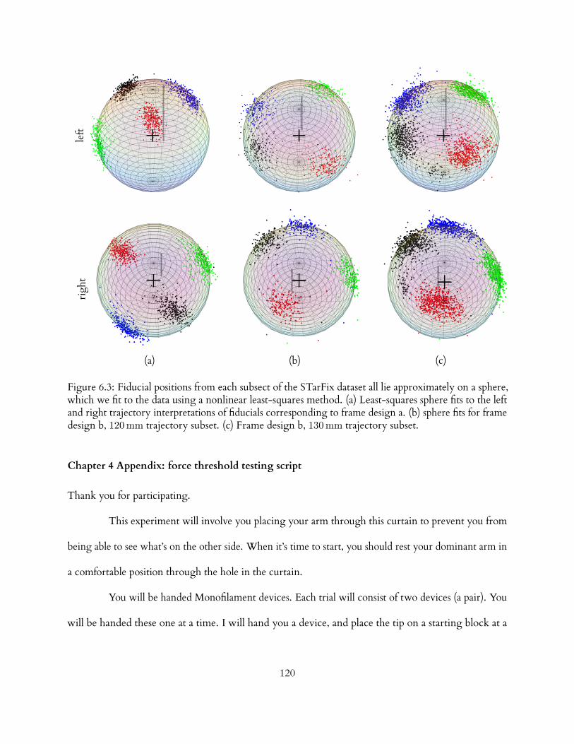
left

righ

t

(a) (b) (c)

Figure 6.3: Fiducial positions from each subsect of the STarFix dataset all lie approximately on a sphere,which we fit to the data using a nonlinear least-squares method. (a) Least-squares sphere fits to the leftand right trajectory interpretations of fiducials corresponding to frame design a. (b) sphere fits for framedesign b, 120 mm trajectory subset. (c) Frame design b, 130 mm trajectory subset.

Chapter 4 Appendix: force threshold testing script

Thank you for participating.

This experiment will involve you placing your arm through this curtain to prevent you from

being able to see what’s on the other side. When it’s time to start, you should rest your dominant arm in

a comfortable position through the hole in the curtain.

You will be handed Monofilament devices. Each trial will consist of two devices (a pair). You

will be handed these one at a time. I will hand you a device, and place the tip on a starting block at a

120

fixed height. This will ensure correct positioning and orientation. When you are ready, I will slide

the starting block away so that you are holding the device without support. At this time, you should

advance the filament straight down, at a speed that you would normally insert a cochlear implant into a

cochleostomy. You should advance continuously downward, without stopping or backing up, until you

reach a mechanical stop that prevents you from advancing any further. While you are advancing, you

should make note of whether or not you feel the filament tip touch the surface prior to reaching the stop.

You should not tell me whether or not you feel anything.

I will then take the first device from your hand, and hand you the second device of the trial. I

will again place it on the starting block. You will perform the exact same task, moving downward at a

continuous speed until hitting the mechanical stop, and take note of whether or not you feel a filament

touch prior to stopping.

In each pair, one of the devices will contain a filament that does touch, and the other will have

no filament, and therefore not make any contact at all. After you complete the pair, I will ask you,“which

one did you feel, the first one, or the second one?”. You must decide (even if it’s a guess), which one you

think you felt, and which one you didn’t.

Do you have any questions about the experiment or what you’ll be asked to do?

We will then repeat this with several other pairs of filaments. Each pair will be done in a random

order. For example, sometimes the first device will have no filament, and sometimes the second device

will have no filament.

Communication between us during the experiment will be limited. I will speak only to tell

you information about the tasks being performed (i.e., “now I’m going to hand you the next filament”),

121

and to ask which filament you felt. You should only answer my questions. I will not be able to answer

any additional questions for you during the experiment, so if you have any questions prior to starting,

please let me know now.

Do you have any additional questions?

You’ll now have 30 seconds to see one of the filaments and practice compressing it on a flat surface. This

is so that you can have an idea of what you’re feeling for.

If you don’t have any further questions, we’ll begin.

122

Chapter 5 Appendix: Permanent Magnet Field Models

A permanent magnet establishes a three-dimensional magnetic field B. To approximate B with the

point-dipole model, a coordinate frame is placed at the magnet center. Let a be a vector from the dipole

to the point of observation, and a a unit vector in the direction of a, then

B(a) =µ0

4π

(3a(a ·m)−m

‖a‖3

)(6.2)

in which µ0 = 4π × 10−7 H/m is the vacuum permeability constant, and m is the magnet’s dipole

moment. See [171, Ch. 5] for derivation.

‖B‖(T)

Distance along x-axis of Magnet (m)0 0.05 0.1 0.15 0.2

0

0.02

0.04

0.06

0.08

0.1Point-dipole modelCube modelMagnetometer

(a) (b)

measurements

Figure 6.4: (a) A planar slice of the three-dimensional vector field of a cube magnet, shown as streamlines.(b) Measurements of the magnitude ‖Bx‖ of the cube magnet used in experiments, taken with a Hall-eect magnetometer, are shown with the field magnitude simulated using the point-dipole and cubemodels.

Furlani [143, Ch. 4] presented a closed-form solution for the magnetic field of a cuboid magnet.

A Cartesian coordinate system is fixed at the centroid of the magnet volume, with the faces of the

magnet orthogonal to the coordinate axes. The distances of the faces from the origin are given in

123

pairs, where subscript 1 denotes a negative distance and subscript 2 denotes a positive distance: (x1, x2),

(y1, y2), (z1, z2). The volume is uniformly magnetized along the z-axis, and has a residual magnetization

M = ‖M‖. At a point (x, y, z), the x component of the field is given by

Bx(x, y, z) =2∑

k=1

2∑m=1

µ0M

4π(−1)k+m ln (F ) (6.3)

in which

F (x, y, z, xm, y1, y2, zk) =(y − y1) + [(x− xm)2 + (y − y1)2 + (z − zk)2]1/2

(y − y2) + [(x− xm)2 + (y − y2)2 + (z − zk)2]1/2(6.4)

The y component is given by

By(x, y, z) =

2∑k=1

2∑m=1

µ0M

4π(−1)k+m ln (H) (6.5)

in which

H(x, y, z, x1, x2, ym, zk) =(x− x1) + [(x− x1)2 + (y − ym)2 + (z − zk)2]1/2

(x− x2) + [(x− x2)2 + (y − ym)2 + (z − zk)2]1/2(6.6)

and the z component is given by

Bz(x, y, z) =µ0M

4π

2∑k=1

2∑n=1

2∑m=1

(−1)k+n+m × tan−1[(x− xn)(y − ym)

(z − zk)G]

(6.7)

in which

G(x, y, z, xn, ym, zk) =1

[(x− xn)2 + (y − ym)2 + (z − zk)2]1/2(6.8)

124

BIBLIOGRAPHY

[1] B. S. Wilson and M. F. Dorman, “Cochlear implants: current designs and future possibilities,”

Journal of Rehabilitation Research & Development, vol. 45, no. 5, pp. 695–730, 2008.

[2] B. K. Swenor, P. Y. Ramulu, J. R. Willis, D. Friedman, and F. R. Lin, “The prevalence of

concurrent hearing and vision impairment in the united states,” JAMA internal medicine, vol. 173,

no. 4, pp. 312–313, 2013.

[3] P. Gildenberg, “General concepts of stereotactic surgery,” in Modern Stereotactic Neurosurgery

(L. Lunsford, ed.), vol. 1 of Topics in neurological surgery, pp. 3–11, Springer US, 1988.

[4] M. Rahman, G. J. Murad, and J. Mocco, “Early history of the stereotactic apparatus in neuro-

surgery,” Neurosurgical focus, vol. 27, no. 3, p. E12, 2009.

[5] A. M. Lozano, P. L. Gildenberg, and R. R. Tasker, Textbook of stereotactic and functional neurosurgery,

vol. 1. Springer Berlin, 2009.

[6] M. Schulder, Handbook of stereotactic and functional neurosurgery, vol. 58. Informa Healthcare, 2003.

[7] S. H. Greenblatt, A history of neurosurgery: in its scientific and professional contexts. Amer Assn of

Neurological Surgeons, 1997.

[8] J. Flickinger, L. Lunsford, D. Kondziolka, and A. Maitz, “Potential human error in setting

stereotactic coordinates for radiosurgery: implications for quality assurance,” International Journal

of Radiation Oncology Biology Physics, vol. 27, no. 2, pp. 397–401, 1993.

[9] G. Widmann, P. Schullian, M. Ortler, and R. Bale, “Frameless stereotactic targeting devices:

125

technical features, targeting errors and clinical results,” The International Journal of Medical Robotics

and Computer Assisted Surgery, vol. 8, no. 1, pp. 1–16, 2012.

[10] D. A. Orringer, A. Golby, and F. Jolesz, “Neuronavigation in the surgical management of brain

tumors: current and future trends,” Expert Review of Medical Devices, vol. 9, no. 5, pp. 491–500,

2012.

[11] Y. Kwoh, I. Reed, J. Chen, H. Shao, T. Truong, and E. Jonckheere, “A new computerized

tomographic-aided robotic stereotaxis system,” Robotics Age, vol. 7, no. 6, pp. 17–22, 1985.

[12] Y. S. Kwoh, J. Hou, E. A. Jonckheere, and S. Hayati, “A robot with improved absolute positioning

accuracy for ct guided stereotactic brain surgery,” Biomedical Engineering, IEEE Transactions on,

vol. 35, no. 2, pp. 153–160, 1988.

[13] J. Troccaz, ed., Medical Robotics. John Wiley & Sons, 2012.

[14] R. A. Beasley, “Medical robots: Current systems and research directions,” Journal of Robotics,

vol. 2012, 2012.

[15] M. Shoham, M. Burman, E. Zehavi, L. Joskowicz, E. Batkilin, and Y. Kunicher, “Bone-mounted

miniature robot for surgical procedures: concept and clinical applications,” IEEE Transactions on

Robotics and Automation, vol. 19, no. 5, pp. 893–901, 2003.

[16] J. M. Fitzpatrick, P. E. Konrad, C. Nickele, E. Cetinkaya, and C. Kao, “Accuracy of customized

miniature stereotactic platforms,” Stereotactic and functional neurosurgery, vol. 83, no. 1, pp. 25–31,

2005.

[17] R. J. Maciunas, R. L. J. Galloway, J. Latimer, C. Cobb, E. Zaccharias, A. Moore, and V. R.

Mandava Stereotactic Funct. Neurosurg., vol. 58, pp. 103–107, 1992.

126

[18] R. J. Maciunas, R. L. Galloway Jr, and J. W. Latimer, “The application accuracy of stereotactic

frames,” Neurosurgery, vol. 35, no. 4, pp. 682–695, 1994.

[19] T. Varma and P. Eldridge, “Use of the neuromate stereotactic robot in a frameless mode for

functional neurosurgery,” The International Journal of Medical Robotics and Computer Assisted

Surgery, vol. 2, no. 2, pp. 107–113, 2006.

[20] S. Ferrand-Sorbets, M. Delphine Taussig, M. Fohlen, C. Bulteau, G. Dorfmuller, and

O. Delalande, “Frameless stereotactic robot-guided placement of depth electrodes for stereo-

electroencephalography in the presurgical evaluation of childrenwith drug-resistant focal epilepsy,”

in CNS Annual Meeting, 2010.

[21] D. P. Devito, L. Kaplan, R. Dietl, M. Pfeier, D. Horne, B. Silberstein, M. Hardenbrook,

G. Kiriyanthan, Y. Barzilay, A. Bruskin, et al., “Clinical acceptance and accuracy assessment of

spinal implants guided with spineassist surgical robot: retrospective study,” Spine, vol. 35, no. 24,

pp. 2109–2115, 2010.

[22] R. Balachandran, J. E. Mitchell, B. M. Dawant, and J. M. Fitzpatrick, “Accuracy evaluation of

microTargeting platforms for deep-brain stimulation using virtual targets,” IEEE Transactions on

Biomedical Engineering, vol. 56, pp. 37–44, January 2009.

[23] L. B. Kratchman, G. S. Blachon, T. J. Withrow, R. Balachandran, R. F. Labadie, and R. J. Webster

III, “Design of a bone-attached parallel robot for percutaneous cochlear implantation,” Biomedical

Engineering, IEEE Transactions on, vol. 58, no. 10, pp. 2904–2910, 2011.

[24] L. B. Kratchman and J. M. Fitzpatrick, “Robotically-adjustable microstereotactic frames for image-

127

guided neurosurgery,” in SPIE Medical Imaging, pp. 86711U–86711U, International Society for

Optics and Photonics, 2013.

[25] R. F. Labadie, R. Balchandran, J. E. Mitchell, J. H. Noble, O. Majdani, D. S. Haynes, M. L.

Bennett, B. M. Dawant, and J. M. Fitzpatrick, “Clinical validation study of percutaneous cochlear

access using patient-customized microstereotactic frames,” Otology & Neurotology, vol. 31(1), no. 1,

pp. 94–99, 2010.

[26] R. Balachandran, J. E. Mitchell, G. S. Blachon, J. H. Noble, B. M. Dawant, J. M. Fitzpatrick, and

R. F. Labadie, “Percutaneous cochlear implant drilling via customized frames: An in vitro study,”

Otolaryngology-Head and Neck Surgery, vol. 142, no. 3, pp. 421–426, 2010.

[27] R. F. Labadie, J. E.Mitchell, R. Balachandran, and J.M. Fitzpatrick, “Customized, rapid-production

microstereotactic table for surgical targeting: description of concept and in vitro validation,”

International Journal of Computer Assisted Radiology and Surgery, vol. 4, no. 3, pp. 273–280, 2009.

[28] J. H. Noble, B. M. Dawant, F. M. Warren, and R. F. Labadie, “Automatic identification and 3D

rendering of temporal bone anatomy,” Otology & Neurotology, vol. 30, no. 4, pp. 436–442, 2009.

[29] J. H. Noble, F. M. Warren, R. F. Labadie, and B. M. Dawant, “Automatic segmentation of the

facial nerve and chorda tympani in ct images using spatially dependent feature values,” Medical

Physics, vol. 35, no. 12, pp. 5375–5384, 2008.

[30] J. H. Noble, F. M. Warren, R. F. Labadie, B. Dawant, and J. M. Fitzpatrick, “Determination of

drill paths for percutaneous cochlear access accounting for target positioning error,” in Proceedings

of SPIE, vol. 6509, pp. 251–263, 2007.

[31] D. Schurzig, R. F. Labadie, A. Hussong, T. S. Rau, and R. J. Webster III, “Design of a Tool

128

Integrating Force Sensing with Automated Insertion in Cochlear Implantation,” IEEE/ASME

Transactions on Mechatronics, vol. 17, no. 2, pp. 381–389, 2012.

[32] L. B. Kratchman, D. Schurzig, T. R. McRackan, R. Balachandran, J. H. Noble, R. J. Webster III,

and R. F. Labadie, “A Manually-Operated, Advance O-Stylet Insertion Tool for Image-Guided,

Minimally Invasive Cochlear Implantation Surgery,” IEEE Transactions on Biomedical Engineering,

vol. 59, no. 10, pp. 2792–2800, 2012.

[33] T. McRackan, R. Balachandran, J. H. Noble, D. Schurzig, G. S. Blachon, J. E. Mitchell, B. M.

Dawant, J. M. Fitzpatrick, and R. F. Labadie, “In-vitro validation of percutaneous cochlear

implantation,” in 2011 Association for Research in Otolaryngology, (Baltimore, MD), Feb. 2011.

[34] O. Majdani, T. A. Schuman, D. S. Haynes, M. S. Dietrich, M. Leinung, T. Lenarz, and R. F.

Labadie, “Time of cochlear implant surgery in academic settings,” Otolaryngology - Head and Neck

Surgery, vol. 142, no. 2, pp. 254–259, 2010.

[35] W. Sukovich, S. Brink-Danan, and M. Hardenbrook, “Miniature robotic guidance for pedicle

screw placement in posterior spinal fusion: early clinical experience with the SpineAssist®,” The

International Journal of Medical Robotics and Computer Assisted Surgery, vol. 2, no. 2, pp. 114–122,

2006.

[36] L. Joskowicz, R. Shamir, M. Freiman, M. Shoham, E. Zehavi, F. Umansky, and Y. Shoshan,

“Image-guided system with miniature robot for precise positioning and targeting in keyhole

neurosurgery,” Computer Aided Surgery, vol. 11, no. 4, p. 181, 2006.

[37] R. Shamir, Z. Israel, M. Shoham, L. Joskowicz, and Y. Shohan, “Renaissance robotic system for

129

keyhole cranial neurosurgery: in vitro accuracy study,” International Journal of Computer Assisted

Radiology and Surgery, vol. 6, pp. 82–89, 2011.

[38] C. Plaskos, P. Cinquin, S. Lavallee, and A. J. Hodgson, “Praxiteles: a miniature bone-mounted

robot for minimal access total knee arthroplasty,” International Journal of Medical Robotics and

Computer Assisted Surgery, vol. 1, no. 4, pp. 67–79, 2005.

[39] S. Song, A. Mor, and B. Jaramaz, “HyBAR: hybrid bone-attached robot for joint arthroplasty,”

The International Journal of Medical Robotics and Computer Assisted Surgery, vol. 5, no. 2, pp. 223–231,

2009.

[40] A. Wolf, B. Jaramaz, B. Lisien, and A. M. DiGioia, “MBARS: mini bone-attached robotic system

for joint arthroplasty,” The International Journal of Medical Robotics and Computer Assisted Surgery,

vol. 1, no. 2, pp. 101–121, 2005.

[41] F. Maes, A. Collignon, D. Vandermeulen, G. Marchal, and P. Suetens, “Multimodality image

registration by maximization of mutual information,” IEEE Transactions on Medical Imaging, vol. 16,

no. 2, pp. 187–198, 1997.

[42] D. Henderson, “Simple Ceramic Motor . . . Inspiring Smaller Products,” in Actuator 2006: 10th

International Conference on New Actuators, (Bremen, Germany), pp. 1–4, 2006.

[43] J. Merlet, Parallel robots. Springer-Verlag New York Inc, 2006.

[44] J.-P. Merlet and D. Daney, “Legs interference checking of parallel robots over a given workspace

or trajectory,” in Robotics and Automation, 2006. Proceedings 2006 IEEE International Conference on,

pp. 757–762, IEEE, 2006.

[45] L. Tsai, Robot analysis: the mechanics of serial and parallel manipulators. Wiley-Interscience, 1999.

130

[46] J. M. Fitzpatrick, D. L. G. Hill, and C. R. Maurer, “Image registration,” in Handbook of Medical

Imaging (M. Sonka and J. Fitzpatrick, eds.), vol. II, ch. 8, pp. 447–513, Bellingham, WA: SPIE,

2000.

[47] B. Bell, N. Gerber, T. Williamson, K. Gavaghan, W. Wimmer, M. Caversaccio, and S. Weber,

“In vitro accuracy evaluation of image-guided robot system for direct cochlear access,” Otology &

Neurotology, vol. 34, no. 7, pp. 1284–1290, 2013.

[48] B. Schrader, W. Hamel, D. Weinert, and H. Mehdorn, “Documentation of electrode localization,”

Movement disorders, vol. 17, no. S3, pp. S167–S174, 2002.

[49] H. Bjartmarz and S. Rehncrona, “Comparison of accuracy and precision between frame-based

and frameless stereotactic navigation for deep brain stimulation electrode implantation,” Stereotactic

and functional neurosurgery, vol. 85, no. 5, pp. 235–242, 2007.

[50] K. Holloway, S. Gaede, P. Starr, J. Rosenow, V. Ramakrishnan, and J. Henderson, “Frameless

stereotaxy using bone fiducial markers for deep brain stimulation,” Journal of neurosurgery, vol. 103,

no. 3, pp. 404–413, 2005.

[51] D. Rajon, F. Bova, and W. Friedman, “Rapid fabrication of custom patient biopsy guides,” Journal

of Applied Clinical Medical Physics, vol. 10, no. 4, pp. 260–272, 2009.

[52] J. Kobler, J. Kotlarski, J. Öltjen, S. Baron, and T. Ortmaier, “Design and analysis of a head-

mounted parallel kinematic device for skull surgery,” International journal of computer assisted

radiology and surgery, vol. 7, no. 1, pp. 137–149, 2012.

[53] J. P. Thiran, R. Charrier, and D. Haag, “The stereopod: an accurate guidance system for frameless

stereotactic neurosurgery,” in CARS 2010, 2010.

131

[54] A. Slocum, “Kinematic couplings for precision fixturing, part 1: Formulation of design parameters,”

Precision Engineering, vol. 10, no. 2, pp. 85–91, 1988.

[55] A. Slocum and A. Donmez, “Kinematic couplings for precision fixturing, part 2: Experimental

determination of repeatability and stiness,” Precision engineering, vol. 10, no. 3, pp. 115–122, 1988.

[56] M. Sonka and J. M. Fitzpatrick, Medical Image Processing and Analysis, Volume II of the Handbook of

Medical Imaging. SPIE Press, 2000.

[57] J. M. Fitzpatrick, R. Balachandran, and G. S. Blachon, “Accuracy validation of waypoint planner

localization for microtable locator spheres,” tech. rep., Vanderbilt University, Dec 2012.

[58] J. M. Fitzpatrick, J. B. West, and C. R. Maurer Jr., “Predicting error in rigid-body point-based

registration,” Medical Imaging, IEEE Transactions on, vol. 17, no. 5, pp. 694–702, 1998.

[59] K. Mardia and P. Jupp, Directional statistics, vol. 494. Wiley, 2009.

[60] B. Mangus, A. Rivas, B. S. Tsai, D. S. Haynes, and J. T. Roland Jr, “Surgical techniques in cochlear

implants,” Otolaryngologic Clinics of North America, vol. 45, no. 1, pp. 69–80, 2012.

[61] R. Brito, T. A. Monteiro, A. F. Leal, R. K. Tsuji, M. H. Pinna, and R. F. Bento, “Surgical

complications in 550 consecutive cochlear implantation,” Brazilian journal of otorhinolaryngology,

vol. 78, no. 3, pp. 80–85, 2012.

[62] A. Aschendor, J. Kromeier, T. Klenzner, and R. Laszig, “Quality control after insertion of

the nucleus contour and contour advance electrode in adults,” Ear and Hearing, vol. 28, no. 2,

pp. 75S–79S, 2007.

[63] M. W. Skinner, T. A. Holden, B. R. Whiting, A. H. Voie, B. Brunsden, J. G. Neely, E. A. Saxon,

T. E. Hullar, and C. C. Finley, “In vivo estimates of the position of advanced bionics electrode

132

arrays in the human cochlea.,” The Annals of otology, rhinology & laryngology. Supplement, vol. 116(4),

pp. 2–24, 2007.

[64] C. C. Finley, T. A. Holden, L. K. Holden, B. R. Whiting, R. A. Chole, G. J. Neely, T. E. Hullar,

and M. W. Skinner, “Role of electrode placement as a contributor to variability in cochlear

implant outcomes,” Otology & Neurotology, vol. 29, no. 7, pp. 920–928, 2008.

[65] G. B. Wanna, J. H. Noble, M. L. Carlson, R. H. Giord, M. S. Dietrich, D. S. Haynes, B. M.

Dawant, and R. F. Labadie, “Impact of electrode design and surgical approach on scalar location

and cochlear implant outcomes,” The Laryngoscope, vol. 124, no. S6, pp. S1–S7, 2014.

[66] O. Adunka and J. Kiefer, “Impact of electrode insertion depth on intracochlear trauma,”

Otolaryngology-Head and Neck Surgery, vol. 135, no. 3, pp. 374–382, 2006.

[67] T. Ishii, M. Takayama, and Y. Takahashi, “Mechanical properties of human round window, basilar

and reissner’s membranes,” Acta Oto-Laryngologica, vol. 115, no. S519, pp. 78–82, 1995.

[68] M. Carlson, C. Driscoll, R. Giord, N. Tombers, B. Hughes-Borst, B. Ne, C. Beatty, et al., “Impli-

cations of minimizing trauma during conventional cochlear implantation,” Otology & Neurotology,

vol. 32, no. 6, pp. 962–968, 2011.

[69] O. Majdani, D. Schurzig, A. Hussong, T. Rau, J. Wittkopf, T. Lenarz, and R. F. Labadie, “Force

measurement of insertion of cochlear implant electrode arrays in vitro: comparison of surgeon to

automated insertion tool,” Acta oto-laryngologica, vol. 130, no. 1, pp. 31–36, 2010.

[70] D. Schurzig, R. J. Webster III, M. S. Dietrich, and R. F. Labadie, “Force of cochlear implant

electrode insertion performed by a robotic insertion tool: comparison of traditional versus advance

o-stylet techniques,” Otology & Neurotology, vol. 31, no. 8, pp. 1207–1210, 2010.

133

[71] L. A. Jones and H. Z. Tan, “Application of psychophysical techniques to haptic research,” Haptics,

IEEE Transactions on, vol. 6, no. 3, pp. 268–284, 2013.

[72] F. Kingdom and N. Prins, “Psychophysics: a practical introduction,” 2010.

[73] G. A. Gescheider, Psychophysics: the fundamentals. Psychology Press, 2013.

[74] N. Prins et al., Psychophysics: a practical introduction. Academic Press, 2009.

[75] M. R. Leek, “Adaptive procedures in psychophysical research,” Perception & psychophysics, vol. 63,

no. 8, pp. 1279–1292, 2001.

[76] M. A. Garcia-Perez, “Forced-choice staircases with fixed step sizes: asymptotic and small-sample

properties,” Vision research, vol. 38, no. 12, pp. 1861–1881, 1998.

[77] H. Levitt, “Transformed up-down methods in psychoacoustics,” The Journal of the Acoustical society

of America, vol. 49, no. 2B, pp. 467–477, 2005.

[78] L. A. Jones, “Perception of force and weight: theory and research.,” Psychological bulletin, vol. 100,

no. 1, p. 29, 1986.

[79] L. A. Jones and S. J. Lederman, Human hand function. Oxford University Press, 2006.

[80] J. Bell-Krotoski and E. Tomancik, “The repeatability of testing with semmes-weinstein monofila-

ments,” The Journal of hand surgery, vol. 12, no. 1, pp. 155–161, 1987.

[81] V. F. Voerman, J. van Egmond, and B. J. Crul, “Normal values for sensory thresholds in the

cervical dermatomes: A critical note on the use of semmes-weinstein monofilaments,” American

journal of physical medicine & rehabilitation, vol. 78, no. 1, pp. 24–29, 1999.

134

[82] J. Dosher and B. Hannaford, “Human interaction with small haptic eects,” Presence: Teleoperators

and Virtual Environments, vol. 14, no. 3, pp. 329–344, 2005.

[83] H. H. King, R. Donlin, and B. Hannaford, “Perceptual thresholds for single vs. multi-finger haptic

interaction,” in Haptics Symposium, 2010 IEEE, pp. 95–99, IEEE, 2010.

[84] G. Baud-Bovy and E. Gatti, “Hand-held object force direction identification thresholds at rest and

during movement,” in Haptics: Generating and Perceiving Tangible Sensations, pp. 231–236, Springer,

2010.

[85] W. E. C. on Leprosy andW. H. Organization,WHO Expert Committee on Leprosy: Seventh Report,

vol. 874. World Health Organization, 1998.

[86] M. H. Haloua, I. Sierevelt, and W. J. Theuvenet, “Semmes-weinstein monofilaments: influence of

temperature, humidity, and age,” The Journal of hand surgery, vol. 36, no. 7, pp. 1191–1196, 2011.

[87] M. J. Mueller, “Identifying patients with diabetes mellitus who are at risk for lower-extremity

complications: use of semmes-weinstein monofilaments,” Physical Therapy, vol. 76, no. 1, pp. 68–71,

1996.

[88] E. H. Tracey, A. J. Greene, and R. L. Doty, “Optimizing reliability and sensitivity of semmes–

weinstein monofilaments for establishing point tactile thresholds,” Physiology & behavior, vol. 105,

no. 4, pp. 982–986, 2012.

[89] M. Zhou, J. Perreault, S. Schwaitzberg, and C. Cao, “Eects of experience on force perception

threshold in minimally invasive surgery,” Surgical endoscopy, vol. 22, no. 2, pp. 510–515, 2008.

[90] N. Gurari and G. Baud-Bovy, “Customization, control, and characterization of a commercial

135

haptic device for high-fidelity rendering of weak forces,” Journal of neuroscience methods, vol. 235,

pp. 169–180, 2014.

[91] N. van de Berg, D. van Gerwen, J. Dankelman, and J. van den Dobbelsteen, “Design choices in

needle steering;a review,” IEEE/ASME Transactions on Mechatronics, In Press.

[92] Y. Fu, H. Liu, W. Huang, S. Wang, and Z. Liang, “Steerable catheters in minimally invasive

vascular surgery,” The International Journal of Medical Robotics and Computer Assisted Surgery, vol. 5,

no. 4, pp. 381–391, 2009.

[93] F. Carpi and C. Pappone, “Stereotaxis niobe magnetic navigation system for endocardial catheter

ablation and gastrointestinal capsule endoscopy.,” Expert Review of Medical Devices, vol. 6, no. 5,

pp. 487–498, 2009.

[94] B. L. Nguyen, J. L. Merino, and E. S. Gang, “Remote navigation for ablation procedures – a

new step forward in the treatment of cardiac arrhythmias,” European Cardiology, vol. 6, no. 3,

pp. 50–56, 2010.

[95] Aeon scientific. [Online]. March, 2015. URL: http://www.aeon-scientific.com

[96] F. Ullrich, S. Schuerle, R. Pieters, A. Dishy, S. Michels, and B. J. Nelson, “Automated capsulorhexis

based on a hybrid magnetic-mechanical actuation system,” in Robotics and Automation (ICRA),

2014 IEEE International Conference on, pp. 4387–4392, IEEE, 2014.

[97] M. P. Kummer, J. J. Abbott, B. E. Kratochvil, R. Borer, A. Sengul, and B. J. Nelson, “Octomag:

An electromagnetic system for 5-DOF wireless micromanipulation,” Robotics, IEEE Transactions

on, vol. 26, no. 6, pp. 1006–1017, 2010.

136

[98] T. Roberts, W. Hassenzahl, S. Hetts, and R. Arenson, “Remote control of catheter tip deflection:

An opportunity for interventional MRI,” Magnetic Resonance in Medicine, vol. 48, no. 6, pp. 1091–

1095, 2002.

[99] F. Settecase, M. S. Sussman, M. W. Wilson, S. Hetts, R. L. Arenson, V. Malba, A. F. Bernhardt,

W. Kucharczyk, and T. P. Roberts, “Magnetically-assisted remote control (MARC) steering of

endovascular catheters for interventional MRI: a model for deflection and design implications,”

Medical physics, vol. 34, no. 8, pp. 3135–3142, 2007.

[100] N. Gudino, J. Heilman, J. Derakhshan, J. Sunshine, J. Duerk, and M. Griswold, “Control of

intravascular catheters using an array of active steering coils,” Medical physics, vol. 38, no. 7,

pp. 4215–4224, 2011.

[101] T. Liu and M. Çavoşoglu, “Three dimensional modeling of an MRI actuated steerable catheter

system,” in 2014 IEEE International Conference on Robotics and Automation (ICRA), pp. 4393–4398,

May 2014.

[102] T. Greigarn and M. C. Çavoşoglu, “Task-space motion planning of MRI-actuated catheters for

catheter ablation of atrial fibrillation,” in 2014 IEEE/RSJ International Conference on Intelligent

Robots and Systems, pp. 3476–3482, IEEE, 2014.

[103] J. R. Clark, L. Leon, F. M. Warren, and J. J. Abbott, “Magnetic guidance of cochlear implants:

Proof-of-concept and initial feasibility study,” Journal of Medical Devices, vol. 6, pp. 035002–035002,

Aug. 2012.

[104] A. W. Mahoney and J. J. Abbott, “5-DOF manipulation of an untethered magnetic device in fluid

using a single permanent magnet,” in Proceedings of Robotics : Science and Systems, July 2014.

137

[105] I. Tunay, “Distributed parameter statics of magnetic catheters,” in 2011 Annual International

Conference of the IEEE Engineering in Medicine and Biology Society, pp. 8344–8347, Aug. 2011.

[106] I. Tunay, “Spatial continuum models of rods undergoing large deformation and inflation,” IEEE

Transactions on Robotics, vol. 29, no. 2, pp. 297–307, 2013.

[107] A. A. Eshraghi, N. W. Yang, and T. J. Balkany, “Comparative study of cochlear damage with

three perimodiolar electrode designs,” The Laryngoscope, vol. 113, no. 3, pp. 415–419, 2003.

[108] C. A. Buchman, J. Joy, A. Hodges, F. F. Telischi, and T. J. Balkany, “Vestibular eects of cochlear

implantation,” The Laryngoscope, vol. 114, no. S103, pp. 1–22, 2004.

[109] P. S. Roland, W. Gstöttner, and O. Adunka, “Method for hearing preservation in cochlear implant

surgery,” Operative Techniques in Otolaryngology-Head and Neck Surgery, vol. 16, no. 2, pp. 93–100,

2005.

[110] P. Roland and C. Wright, “Surgical aspects of cochlear implantation: mechanisms of insertional

trauma,” Advances in Otorhinolaryngology, vol. 64, no. R, p. 11, 2006.

[111] P. Wardrop, D. Whinney, S. J. Rebscher, J. T. Roland, W. Luxford, and P. A. Leake, “A

temporal bone study of insertion trauma and intracochlear position of cochlear implant electrodes.

i: Comparison of nucleus banded and nucleus contour electrodes,” Hearing research, vol. 203, no. 1,

pp. 54–67, 2005.

[112] P. Wardrop, D. Whinney, S. J. Rebscher, W. Luxford, and P. Leake, “A temporal bone study of

insertion trauma and intracochlear position of cochlear implant electrodes. ii: comparison of spiral

clarion and hifocus ii electrodes,” Hearing research, vol. 203, no. 1, pp. 68–79, 2005.

138

[113] O. F. A. H. C. Pillsbury and C. A. Buchman, “Minimizing intracochlear trauma during cochlear

implantation,” Cochlear Implants and Hearing Preservation, vol. 67, pp. 96–107, 2009.

[114] C. G. Wright, P. S. Roland, et al., “Vascular trauma during cochlear implantation: A contributor

to residual hearing loss?,” Otology & neurotology: ocial publication of the American Otological Society,

American Neurotology Society [and] European Academy of Otology and Neurotology, 2012.

[115] C. A. von Ilberg, U. Baumann, J. Kiefer, J. Tillein, and O. F. Adunka, “Electric-acoustic stim-

ulation of the auditory system: a review of the first decade,” Audiology and Neurotology, vol. 16,

no. supplement 2, pp. 1–30, 2011.

[116] O. Adunka, H. Pillsbury, and C. Buchman, “Minimizing intracochlear trauma during cochlear

implantation,” Advances in Otorhinolaryngoly, vol. 67, pp. 96–107, 2010.

[117] J. Zhang, J. T. Roland, S. Manolidis, and N. Simaan, “Optimal path planning for robotic insertion

of steerable electrode arrays in cochlear implant surgery,” Journal of medical devices, vol. 3, no. 1,

2009.

[118] X. Meshik, T. A. Holden, R. A. Chole, and T. E. Hullar, “Optimal cochlear implant insertion

vectors,” Otology & neurotology: ocial publication of the American Otological Society, American

Neurotology Society [and] European Academy of Otology and Neurotology, vol. 31, no. 1, p. 58, 2010.

[119] M. Cosetti and J. T. Roland Jr, “Cochlear implant electrode insertion,” Operative Techniques in

Otolaryngology-Head and Neck Surgery, vol. 21, no. 4, pp. 223–232, 2010.

[120] A. Hussong, T. S. Rau, T. Ortmaier, B. Heimann, T. Lenarz, and O. Majdani, “An automated

insertion tool for cochlear implants: another step towards atraumatic cochlear implant surgery,”

International journal of computer assisted radiology and surgery, vol. 5, no. 2, pp. 163–171, 2010.

139

[121] T. Rau, A. Hussong, M. Leinung, T. Lenarz, and O. Majdani, “Automated insertion of preformed

cochlear implant electrodes: evaluation of curling behaviour and insertion forces on an artificial

cochlear model,” International Journal of Computer Assisted Radiology and Surgery, vol. 5, no. 2,

pp. 173–181, 2010.

[122] J. Zhang, W. Wei, J. Ding, J. T. Roland Jr, S. Manolidis, and N. Simaan, “Inroads toward robot-

assisted cochlear implant surgery using steerable electrode arrays,” Otology & Neurotology, vol. 31,

no. 8, pp. 1199–1206, 2010.

[123] J. Pile, M. Y. Cheung, J. Zhang, and N. Simaan, “Algorithms and design considerations for robot

assisted insertion of perimodiolar electrode arrays,” in Robotics and Automation (ICRA), 2011 IEEE

International Conference on, pp. 2898–2904, IEEE, 2011.

[124] J. Pile and N. Simaan, “Modeling, design, and evaluation of a parallel robot for cochlear implant

surgery (in press),” IEEE Transactions on Mechatronics.

[125] B. Arcand, P. Bhatti, N. Butala, J. Wang, C. Friedrich, and K. Wise, “Active positioning device

for a perimodiolar cochlear electrode array,”Microsystem technologies, vol. 10, no. 6-7, pp. 478–483,

2004.

[126] B. Chen, H. Kha, and G. Clark, “Development of a steerable cochlear implant electrode array,” in

3rd Kuala Lumpur International Conference on Biomedical Engineering 2006, pp. 607–610, Springer,

2007.

[127] J. Wu, L. Yan, H. Xu, W. C. Tang, and F.-G. Zeng, “A curvature-controlled 3d micro-electrode

array for cochlear implants,” in Solid-State Sensors, Actuators and Microsystems, 2005. Digest of

140

Technical Papers. TRANSDUCERS’05. The 13th International Conference on, vol. 2, pp. 1636–1639,

IEEE, 2005.

[128] F. Zeng, S. Rebscher, W. Harrison, X. Sun, and H. Feng, “Cochlear implants: System design,

integration, and evaluation,” IEEE Reviews in Biomedical Engineering, vol. 1, pp. 115–142, 2008.

[129] E. Erixon, H. Högstorp, K. Wadin, and H. Rask-Andersen, “Variational anatomy of the human

cochlea: implications for cochlear implantation,” Otology & Neurotology, vol. 30, no. 1, pp. 14–22,

2009.

[130] J. H. Noble, R. B. Rutherford, R. F. Labadie, O. Majdani, and B. M. Dawant, “Modeling and

segmentation of intra-cochlear anatomy in conventional ct,” in SPIE Medical Imaging, pp. 762302–

762302, International Society for Optics and Photonics, 2010.

[131] R. Martinez-Monedero, J. K. Niparko, and N. Aygun, “Cochlear coiling pattern and orientation

dierences in cochlear implant candidates,” Otology & Neurotology, vol. 32, no. 7, pp. 1086–1093,

2011.

[132] E. Avci, T. Nauwelaers, T. Lenarz, V. Hamacher, and A. Kral, “Variations in microanatomy of

the human cochlea,” Journal of Comparative Neurology, vol. 522, no. 14, pp. 3245–3261, 2014.

[133] K. S. van der Marel, J. J. Briaire, R. Wolterbeek, J. Snel-Bongers, B. M. Verbist, and J. H. Frijns,

“Diversity in cochlear morphology and its influence on cochlear implant electrode position,” Ear

and hearing, vol. 35, no. 1, pp. e9–e20, 2014.

[134] D. Attali, J.-D. Boissonnat, and H. Edelsbrunner, “Stability and computation of medial axes-a

state-of-the-art report,” in Mathematical foundations of scientific visualization, computer graphics, and

massive data exploration, pp. 109–125, Springer, 2009.

141

[135] M.Negahdar, A. Ahmadian, N.Navab, andK. Firouznia, “Path planning for virtual bronchoscopy,”

in Engineering in Medicine and Biology Society, 2006. EMBS’06. 28th Annual International Conference

of the IEEE, pp. 156–159, IEEE, 2006.

[136] D. S. Paik, C. F. Beaulieu, R. B. Jerey, G. D. Rubin, and S. Napel, “Automated flight path

planning for virtual endoscopy,” Medical Physics, vol. 25, p. 629, 1998.

[137] B. M. Verbist, L. Ferrarini, J. J. Briaire, A. Zarowski, F. Admiraal-Behloul, H. Olofsen, J. H.

Reiber, and J. H. Frijns, “Anatomic considerations of cochlear morphology and its implications for

insertion trauma in cochlear implant surgery,” Otology & Neurotology, vol. 30, no. 4, pp. 471–477,

2009.

[138] C. H. Reinsch, “Smoothing by spline functions,”Numerische mathematik, vol. 10, no. 3, pp. 177–183,

1967.

[139] J. Zhang andN. Simaan, “Design of underactuated steerable electrode arrays for optimal insertions,”

Journal of Mechanisms and Robotics, vol. 5(1), p. 011008, January 2013.

[140] D. C. Jiles, Introduction to Magnetism and Magnetic Materials. CRC Press, 1998.

[141] A. Petruska and J. Abbott, “Optimal permanent-magnet geometries for dipole field approximation,”

Magnetics, IEEE Transactions on, vol. 49, no. 2, pp. 811–819, 2013.

[142] N. Derby and S. Olbert, “Cylindrical magnets and ideal solenoids,” American Journal of Physics,

vol. 78, no. 3, pp. 229–235, 2010.

[143] E. P. Furlani, Permanent Magnet and Electromechanical Devices: Materials, Analysis, and Applications.

Academic Press, 2001.

142

[144] H. E. Knoepfel, Magnetic Fields: a Comprehensive Theoretical Treatise for Practical Use. John Wiley

& Sons, 2008.

[145] G. Kirchho, “Über das gleichgewicht und die bewegung eines unendlich dünnen elastischen

stabes.,” Journal für die reine und angewandte Mathematik, vol. 56, pp. 285–313, 1859.

[146] G. Kirchho, Vorlesungen uber Mathematische Physik. Mechanik, vol. 28. Druck und verlag von BG

Teubner, 1876.

[147] E. H. Dill, “Kirchho’s theory of rods,” Archive for History of Exact Sciences, vol. 44, no. 1, pp. 1–23,

1992.

[148] S. S. Antman, Nonlinear Problems of Elasticity. Springer New York, 2 ed., 2005.

[149] B. Audoly and Y. Pomeau, Elasticity and geometry: From Hair Curls to the Nonlinear Response of

Shells. Oxford Univ. Press, 2010.

[150] D. C. Rucker, B. A. Jones, and Robert J Webster III, “A geometrically exact model for externally

loaded concentric-tube continuum robots,” IEEE Transactions on Robotics, vol. 26, pp. 769–780,

Oct. 2010.

[151] B. O’neill, Elementary dierential geometry. Academic press, 2006.

[152] A. J. Hanson, Visualizing Quaternions. Morgan Kaufmann Series in Interactive 3D Technology,

Morgan Kaufmann/Elsevier, 1 ed., 2005.

[153] W. Wang, B. Jüttler, D. Zheng, and Y. Liu, “Computation of rotation minimizing frames,” ACM

Transactions on Graphics (TOG), vol. 27, no. 1, p. 2, 2008.

143

[154] E. H. Dill, “The shear center and kirchho’s theory of rods,” tech. rep., Rutgers University,

Center for Computational Modeling of Aircraft Structures, December 1993.

[155] J. Kierzenka and L. F. Shampine, “A BVP solver that controls residual and error,” Journal of

Numerical Analysis, Industrial and Applied Mathematics, vol. 3, pp. 27–41, 2008.

[156] U. M. Ascher, R. M. Mattheij, and R. D. Russell, Numerical solution of boundary value problems for

ordinary dierential equations. Series in Computational Mathematics, Prentice-Hall, 1988.

[157] A. Ben-Israel and T. N. Greville, Generalized Inverses, vol. 13. Springer, 2003.

[158] T. F. Chan and R. V. Dubey, “A weighted least-norm solution based scheme for avoiding joint

limits for redundant joint manipulators,” Robotics and Automation, IEEE Transactions on, vol. 11,

no. 2, pp. 286–292, 1995.

[159] J. Park, Y. Choi, W. K. Chung, and Y. Youm, “Multiple tasks kinematics using weighted pseudo-

inverse for kinematically redundant manipulators,” in International Conference on Robotics and

Automation, pp. 4041–4047, 2001.

[160] J. Xiang, C. Zhong, andW.Wei, “A varied weights method for the kinematic control of redundant

manipulators with multiple constraints,” Robotics, IEEE Transactions on, vol. 28, no. 2, pp. 330–340,

2012.

[161] O. Khatib, “Real-time obstacle avoidance for manipulators and mobile robots,” The international

journal of robotics research, vol. 5, no. 1, pp. 90–98, 1986.

[162] D. E. Whitney, “Resolved motion rate control of manipulators and human prostheses.,” IEEE

Transactions on man-machine systems, 1969.

144

[163] P. Chiacchio, S. Chiaverini, L. Sciavicco, and B. Siciliano, “Closed-loop inverse kinematics

schemes for constrained redundant manipulators with task space augmentation and task priority

strategy,” The International Journal of Robotics Research, vol. 10, no. 4, pp. 410–425, 1991.

[164] G. Bradski, “OpenCV,” Dr. Dobb’s Journal of Software Tools, 2000.

[165] R. I. Hartley and P. Sturm, “Triangulation,” Computer vision and image understanding, vol. 68, no. 2,

pp. 146–157, 1997.

[166] H. S. M. Coxeter, Introduction to Geometry. New York, London, 1961.

[167] M. J. Troughton, Handbook of plastics joining: a practical guide. William Andrew, 2008.

[168] R. J. Wise, Thermal welding of polymers. Woodhead Publishing, 1999.

[169] D. Stavrov and H. Bersee, “Resistance welding of thermoplastic composites-an overview,” Com-

posites Part A: Applied Science and Manufacturing, vol. 36, no. 1, pp. 39–54, 2005.

[170] C. M. Shakarji, “Least-squares fitting algorithms of the NIST algorithm testing system,” Journal

of Research–National Institute of Standards and Technology, vol. 103, pp. 633–641, 1998.

[171] J. D. Jackson, Classical Electrodynamics, vol. 3. Wiley New York etc., 1962.

145