Embed Size (px)
Citation preview
www.iap.uni-jena.de
Imaging and Aberration Theory
Lecture 12: Zernike polynomials
2014-01-30
Herbert Gross
Winter term 2013

2
Preliminary time schedule
1 24.10. Paraxial imaging paraxial optics, fundamental laws of geometrical imaging, compound systems
2 07.11. Pupils, Fourier optics, Hamiltonian coordinates
pupil definition, basic Fourier relationship, phase space, analogy optics and mechanics, Hamiltonian coordinates
3 14.11. Eikonal Fermat Principle, stationary phase, Eikonals, relation rays-waves, geometrical approximation, inhomogeneous media
4 21.11. Aberration expansion single surface, general Taylor expansion, representations, various orders, stop shift formulas
5 28.11. Representations of aberrations different types of representations, fields of application, limitations and pitfalls, measurement of aberrations
6 05.12. Spherical aberration phenomenology, sph-free surfaces, skew spherical, correction of sph, aspherical surfaces, higher orders
7 12.12. Distortion and coma phenomenology, relation to sine condition, aplanatic sytems, effect of stop position, various topics, correction options
8 19.12. Astigmatism and curvature phenomenology, Coddington equations, Petzval law, correction options
9 09.01. Chromatical aberrations
Dispersion, axial chromatical aberration, transverse chromatical aberration, spherochromatism, secondary spoectrum
10 16.01. Further reading on aberrations sensitivity in 3rd order, structure of a system, analysis of optical systems, lens contributions, Sine condition, isoplanatism, sine condition, Herschel condition, relation to coma and shift invariance, pupil aberrations, relation to Fourier optics
11 23.01. Wave aberrations definition, various expansion forms, propagation of wave aberrations, relation to PSF and OTF
12 30.01. Zernike polynomials special expansion for circular symmetry, problems, calculation, optimal balancing, influence of normalization, recalculation for offset, ellipticity, measurement
13 06.02. Miscellaneous Intrinsic and induced aberrations, Aldi theorem, vectorial aberrations, partial symmetric systems

1. Definition
2. Properties
3. Calculation
4. Application in optical performance description
5. Aberration balancing
6. Sampling
7. Relation to power expansion
8. Change influences
9. High NA case
10. Miscellaneous
3
Contents

Zernike Polynomials
+ 6
+ 7
- 8
m = + 8
0 5 8764321n =
cos
sin
+ 5
+ 4
+ 3
+ 2
+ 1
0
- 1
- 2
- 3
- 4
- 5
- 6
- 7
Expansion of wave aberration surface into elementary functions / shapes
Zernike functions are defined in circular coordinates r,
Ordering of the Zernike polynomials by indices:
n : radial
m : azimuthal, sin/cos
Mathematically orthonormal function on unit circle for a constant weighting function
Direct relation to primary aberration types
n
n
nm
m
nnm rZcrW ),(),(
01
0)(cos
0)(sin
)(),(
mfor
mform
mform
rRrZ m
n
m
n
4

Zernike Polynomials
Alternative representation
5
+ 6
+ 7
- 8
m = + 8
0 5 8764321n =
cos
sin
+ 5
+ 4
+ 3
+ 2
+ 1
0
- 1
- 2
- 3
- 4
- 5
- 6
- 7
yp
xp

Zernike Polynomials
Advantages of the Zernike polynomials:
1. usually good match of circular symmetry to most optical systems
2. de-coupling of coefficients due to orthogonality
3. stable numerical computation 4. direct measurement by interferometry possible
5. direct relation of lower orders to classical aberrations
6. optimale balancing of lower orders (e.g. best defocus for spherical aberration)
7. fast calculation of Wrms and Strehl ratio in approximation of Marechal
Problems and disadvantages of the Zernike polynomials:
1. computation on discrete grids
2. non circular pupils often occur in practice
3. different conventions can be found, conversion is quite confusing
4. calculation not stable for very high orders
5. Zernike functions are no eigenfunctions of wave propagation,
if the measurement is not made exactly in the pupil, the coefficients are erroneous
6

Indexing and Azimuthal Periodicity
azimuthal index m
radial
index n
same
spatial
frequency
rotational
symmetry:
defocus
spherical
in cosq
linear :
tilt, coma
in cos2q
quadratic :
astigmatisms
empty
in cos3q of
3rd power :
trefoil
Index m: azimuthal periodicity
Constant spatial frequency: sum of n+|m|
7

Nr Cartesian representation Circular representation
1 1 1
2 x r sin
3 y r cos
4 2 x2 + 2 y
2 - 1 2 r² - 1
5 2 x y r² sin 2
6 y2 - x
2 r² cos 2
7 ( 3x2 + 3 y
2 - 2 ) x ( 3r
3 - 2r ) sin
8 ( 3x2 + 3 y
2 - 2 ) y ( 3r
3 - 2r ) cos
9 6 (x2+y
2)2-6 (x
2+y
2) +1 6r
4 - 6r² + 1
10 ( 3y2-x
2 ) x r³ sin 3
11 ( y2-3x
2) y r³ cos 3
12 (4x2+4y
2-3) 2xy ( 4r
4 - 3r² ) sin 2
13 (4x2+4y
2-3) (y
2 - x
2) ( 4r
4 - 3r² ) cos 2
14 [10(x2+y
2)2-12(x
2+y
2)+3] x ( 10r
5 - 12r³ + 3r ) sin
15 [10(x2+y
2)2-12(x
2+y
2)+3] y ( 10r
5 - 12r³ + 3r ) cos
16 20 (x2+y
2)3 - 30 (x
2+y
2)2 + 12 (x
2+y
2) - 1 20r
6 - 30r
4 + 12r² - 1
17 (y2-x
2) 4xy R
4 sin 4
18 y4+x
4-6x
2y
2 R
4 cos 4
Zernike Polynomials: Fringe Convention
8

19 (5x2+5y
2-4) (3y
2-x
2)x ( 5r
5 - 4r³ ) sin 3
20 (5x2+5y
2-4) (y
2-3x
2)y ( 5r
5 - 4r³ ) cos 3
21 [15(x2+y
2)2-20(x
2+y
2)+6] 2xy ( 15r
6 - 20r
4 + 6r² ) sin 2
22 [15(x2+y
2)2-20(x
2+y
2)+6] (y
2-x
2) ( 15r
6 - 20r
4 + 6r² ) cos 2
23 [35(x2+y
2)3-60(x
2+y
2)2+30(x
2+y
2)-4] x ( 35r
7 - 60r
5 + 30r³ - 4r ) sin
24 [35(x2+y
2)3-60(x
2+y
2)2+30(x
2+y
2)-4] y ( 35r
7 - 60r
5 + 30r³ - 4r ) cos
25 70(x2+y
2)4-140(x
2+y
2)3+90(x
2+y
2)2-20(x
2+y
2)+1 70r
8 - 140r
6 + 90r
4 - 20r² + 1
26 (5y4-10x
2y
2+x
4)x R
5 sin 5
27 (y4-10x
2y
2+5x
4)y R
5 cos 5
28 (6x2+6y
2-5) (y
2-x
2)2xy ( 6r
6 - 5r
4 ) sin 4
29 (6x2+6y
2-5) (y
4-6x
2y
2+x
4) ( 6r
6 - 5r
4 ) cos 4
30 [21(x2+y
2)2-30(x
2+y
2)+10] (3y
2-x
2)x ( 21r
7 - 30r
5 + 10r
3 ) sin 3
31 [21(x2+y
2)2-30(x
2+y
2)+10] (y
2-3x
2)y ( 21r
7 - 30r
5 + 10r
3 ) cos 3
32 [ 56(x2+y
2)3-105(x
2+y
2)2+60(x
2+y
2)-10] 2xy ( 56r
8 – 105r
6 + 60r
4 - 10r
2 ) sin 2
33 [ 56(x2+y
2)3-105(x
2+y
2)2+60(x
2+y
2)-10] (y
2-x
2) ( 56r
8 – 105r
6 + 60r
4 - 10r
2 ) cos 2
34 [ 126(x2+y
2)4-280(x
2+y
2)3+210(x
2+y
2)2-60(x
2+y
2)+5] x ( 126r
9 – 280r
7 + 210r
5 – 60r
3 + 5r ) sin
35 [ 126(x2+y
2)4-280(x
2+y
2)3+210(x
2+y
2)2-60(x
2+y
2)+5] y ( 126r
9 – 280r
7 + 210r
5 – 60r
3 + 5r ) cos
36 252(x2+y
2)5-630(x
2+y
2)4+560(x
2+y
2)3-
210(x2+y
2)2+30(x
2+y
2)-1
( 252r10
– 630r8 + 560r
6 – 210r
4 + 30r
2 - 1 )
Zernike Polynomials: Fringe Convention
9

Zernike Polynomials: Meaning of Lower Orders
n m Polar coordinates
Interpretation
0 0 1 1 piston
1 1 r sin x
Four sheet 22.5°
1 - 1 r cos y
2 2 r 2
2 sin 2 xy
2 0 2 1 2
r 2 2 1 2 2
x y +
2 - 2 r 2
2 cos y x 2 2
3 3 r 3
3 sin 3 2 3
xy x
3 1 ( ) 3 2 3
r r sin 3 2 3 3 2
x x xy +
3 - 1 ( ) 3 2 3
r r cos 3 2 3 3 2
y y x y +
3 - 3 r 3
3 cos y x y 3 2
3
4 4 r 4
4 sin 4 4 3 3
xy x y
4 2 ( ) 4 3 2 4 2
r r sin 8 8 6 3 3
xy x y xy +
4 0 6 6 1 4 2
r r + 6 6 12 6 6 1 4 4 2 2 2 2 x y x y x y + + +
4 - 2 ( ) 4 3 2 4 2
r r cos 4 4 3 3 4 4 4 2 2 2 2
y x x y x y +
4 - 4 r 4
4 cos y x x y 4 4 2 2
6 +
Cartesian coordinates
tilt in y
tilt in x
Astigmatism 45°
defocussing
Astigmatism 0°
trefoil 30°
trefoil 0°
coma x
coma y
Secondary astigmatism
Secondary astigmatism
Spherical aberration
Four sheet 0°
10

Radial Zernike Polynomials
11
1901980184809009025225242042041184021879048620)(
172126092403465072072840845148012870)(
15675642001155016632120123432)(
142420168031502772924)(
130210560630252)(
1209014070)(
1123020)(
166)(
12)(
24681012141618
100
246810121416
81
2468101214
64
24681012
49
246810
36
2468
25
246
16
24
9
2
4
++++
++++
+++
+++
++
++
+
+
rrrrrrrrrrZ
rrrrrrrrrZ
rrrrrrrrZ
rrrrrrrZ
rrrrrrZ
rrrrrZ
rrrrZ
rrrZ
rrZ
Radial polynomial functions
Oscillating signs corresponds to compensating effects
Large coefficients for higher orders cause numerical inaccuracies for explicite calculations in particular for points near to the edge
Recurence formulas preferred, but residual errors are propagated

Indices of Zernike Fringe Polynomials
Indexing of Fringe polynomials
Principle: growing spatial frequency of variations
1. radial
2. azimuthal
Meaningful: truncation at quadratic numbers
4: image location
9: 4th order, primary aberrations
16: 6th order, secondary aberrations
.....
Indexing:
1. starting with m=0
2. growing absolute value of m
Running index
2
)sgn(121
2
2
mm
mnj
+
+
+
12

Indices of Zernike Fringe Polynomials
13

Zernike Standard Polynomials
Normalization of standard Zernike
polynomials
Orthogonality
Constant rms-value for all terms
easy estimation possible
Indexing of standard polynomials:
1. increasing radial index n
2. increasing absolut value of azimuthal index |m|
Therefore irregulary
growing spatial
frequency
''
'*
'
1
0
2
0
),(),( mmnn
m
n
m
n drrdrZrZ
( )( )
+
+
01
0cos
0sin
)(1
)1(2),(
0mfor
mform
mform
rRn
rZ m
n
m
m
n q
q
q
k
n
n
nm
nmrms cW1
22
sin cos
n/m -10 -9 -8 -7 -6 -5 -4 -3 -2 -1 0 1 2 3 4 5 6 7 8 9 10
0 1
1 2 3
2 5 4 6
3 9 7 8 10
4 14 12 11 13 15
5 20 18 16 17 19 21
6 27 25 23 22 24 26 28
7 35 33 31 29 30 32 34 36
8 44 42 40 38 37 39 41 43 45
14
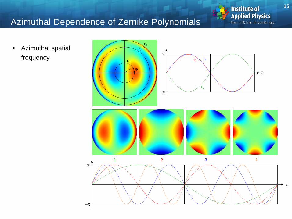
Azimuthal Dependence of Zernike Polynomials
Azimuthal spatial
frequency
r1
r3
r2
r1r3
r2
31
2 4
15

( )''
0'*
'
1
0
2
0)1(2
1),(),( mmnn
mm
n
m
nn
drrdrZrZ
+
+
n
n
nm
m
nnm rZcrW ),(),(
( ) +
+
1
0
*
2
00
),(),(1
)1(2drrdrZrW
nc m
n
m
nm
Orthogonality
Expansion of the wave aberration on a circular area
Orthonormality for Fringe
convention
Orthogonality of radial functions
Determination of coefficients
Necessary requirements for orthogonality:
1. pupil shape circular
2. uniform illumination of pupil (corresponds to constant weighting)
3. no discretization effects (finite number of points, boundary)
Orthogonality perturbed in reality by:
1. real non-circular boundary (vignetting)
2. apodization (laser illumination)
3. discretization (calculation by a discrete finite ray set) ,
16
R r R r r drn
n
m
n
m nn( ) ( )( )
''
+
2 10
1

Orthogonality
Usual found new sets of orthogonal functions:
1. discretized finite sampling grid
2. apodization due to gaussian illumination (Mahajan)
3. elliptical deformed pupil shape (Dai)
4. ring-shaped pupil (Tatian)
5. rectangular pupil (2D Legendre)
General orthogonalization of polynomials by Gram-Schmidt algorithm from Zernikes
possible:
- Definition of inner product of two functions
- first new function Y, normalized
- second new function, linear combination of
old function and lower order new functions
normalized
- general step, analogoues
17
rdrdFFFF 2121
1,
11' ZY 11
11
,
'
YY
YY
YYZZYTZY + 12212122 ,'
22
22
,
'
YY
YY
+1
1
1
1
,'n
m
mmnn
n
m
mnmnn YYZZYTZY
nn
nn
YY
YY
,
'

Mathematical Properties
Recurrence formulas
Explicite formula
Symmetry
Value at the edge
Value range:
18
1
1
1
1 )()2()1(2 +
+
+ ++++ m
n
m
n
m
n RmnRmnRrn
+
+
++
+
+ +
m
n
m
n
m
n Rn
mnR
n
mn
n
mnrn
mn
nR 2
22222
2222
)2()()1(4
)2(
2
qn
mn
q
qm
n r
qmn
qmn
q
qnrR 2
2
0 !2
!2
!
)!()1()(
+
R Rn
m
n
m
Rn
m( )1 1
1...1)1( +m
nZ

Mathematical Properties
Fourier transform relationship:
frequency spectrum of Zernike
functions
Distributed frequency
content
Higher radial order polynomials
has higher spatial frequency
support
In the spatial domain, the high
frequency are located at the
edge
19
( )
( )
( )
+
0)1(
0sin)1(
0cos)1(
)2(,),(ˆ
2
2
2
1
mfor
mformi
mformi
k
kJkUrZF
n
mn
m
mn
m
nnmnm
0 2 4 6 8 10 12-0.2
-0.1
0
0.1
0.2
0.3
0.4
0.5
0.6
0.7
n = 2
n = 6
n = 10
n = 16
n = 24

Different standardizations used concerning:
1. indexing
2. scaling / normalization
3. sign of coordinates (orientation for off-axis field points)
Fringe - representation
1. CodeV, Zemax, interferometric test of surfaces
2. Standardization of the boundary to ±1
3. no additional prefactors in the polynomial
4. Indexing according to m (Azimuth), quadratic number terms have circular symmetry
5. coordinate system invariant in azimuth
Standard - representation
- CodeV, Zemax, Born / Wolf
- Standardization of rms-value on ±1 (with prefactors), easy to calculate Strehl ratio
- coordinate system invariant in azimuth
Original - Nijboer - representation
- Expansion:
- Standardization of rms-value on ±1
- coordinate system rotates in azimuth according to field point
+++k
n
n
gerademn
m
m
nnm
k
n
n
gerademn
m
m
nnm
k
n
nn mRbmRaRaarW0 10 10
0
000 )sin()cos(2
1),(
Zernikepolynomials: Different Conventions
20
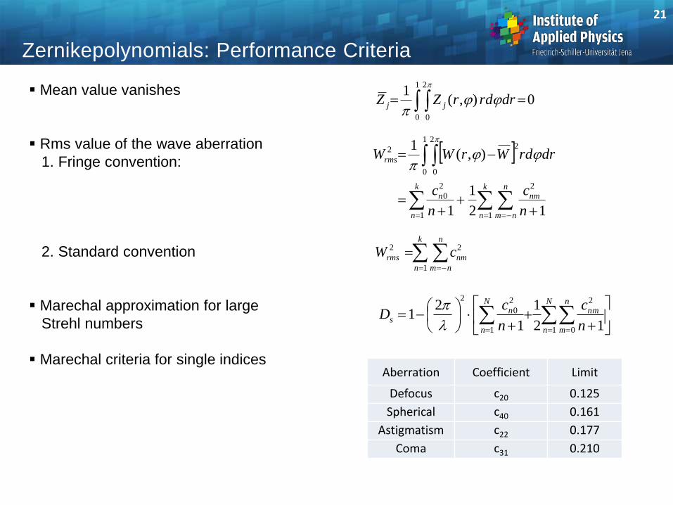
Mean value vanishes
Rms value of the wave aberration 1. Fringe convention:
2. Standard convention
Marechal approximation for large Strehl numbers
Marechal criteria for single indices
Zernikepolynomials: Performance Criteria
21
++
+
k
n
n
nm
nmk
n
n
rms
n
c
n
c
drdrWrWW
1
2
1
2
0
1
0
2
0
22
12
1
1
),(1
k
n
n
nm
nmrms cW1
22
0),(1
1
0
2
0
drdrrZZ jj
++
+
N
n
n
m
nmN
n
ns
n
c
n
cD
1 0
2
1
2
0
2
12
1
1
21
Aberration Coefficient Limit
Defocus c20 0.125
Spherical c40 0.161
Astigmatism c22 0.177
Coma c31 0.210

W
rp1
4th order
(Seidel)
4th and 2nd order
4th, 2nd and 0th order
(Zernike) rms is minimal
4
1
-1
3
2
0_
++ +
_
-2
166)( 24 + ppp rrrW
Balance of Lower Orders by Zernike Polynomials
Mixing of lower orders to get the minimal Wrms
Example spherical aberration:
1. Spherical 4th order according to
Seidel
2. Additional quadratic expression:
Optimal defocussing for edge
correction
3. Additional absolute term
Minimale value of Wrms
Special case of coma: Balancing by tilt contribution, corresponds to shift between peak and centroid
22

drrdrZrWc jj
),(*),(1
1
0
2
0
min)(
2
1 1
i
ijj
N
j
i rZcW
( ) WZZZcTT 1
Calculation of Zernike Polynomials
Assumptions:
1. Pupil circular
2. Illumination homogeneous
3. Neglectible discretization effects /sampling, boundary)
Direct computation by double integral:
1. Time consuming
2. Errors due to discrete boundary shape
3. Wrong for non circular areas
4. Independent coefficients
LSQ-fit computation:
1. Fast, all coefficients cj simultaneously obtained
2. Better total approximation
3. Non stable for different numbers of coefficients,
if number too low
4. Stable for non circular shape of pupil
Calculation by Fourier transform
23
1
22),(),(r
kri rderWkA
q
1
0
*
2
),(),(1 N
l
nmlnm kUkAc qq
rderZkU kri
nmnm
22),(),( q

Radial Sampling
Spatial frequency grows towards the edge of the pupil radius
The outer zeros are denser distributed and grows with index n
The sampling is dominated at the edge
Possible maximum radial order for a given equidistant sampling number N
24
00.
1
0.
2
0.
3
0.
4
0.
5
0.
6
0.
7
0.
8
0.
91
-
1
-
0.8
-
0.6
-
0.4
-
0.2
0
0.
2
0.
4
0.
6
0.
8
1
r
0 0.1 0.2 0.3 0.4 0.5 0.6 0.7 0.8 0.9 10
5
10
15
20
25
30
n = 30
Z(r)
rn
r
zeros
2
)( 1
nr zero
N over
radius
N over
diameter n
32 64 4
64 128 5
128 256 8
256 512 11
512 1024 16

Truncation Error
If the series expansion is truncated before convergence is obtained: - errors in wavefront description - errors of lower order coefficients for NLSQ-calculation:
balancing to minimize the rms-error
Example: - circular symmetric wavefront
- coefficients c4=c9=c16=... = 0.2
- error of lower order coefficients c9, c16 for growing number of terms
25
c/c
0 2 4 6 8 10 12 140
0.1
0.2
0.3
c9
c16

drrdrZrZC jjjj
),(*),(1
1
0
2
0
''
Calculation of Zernike Polynomials
Correlation of modes
Numerical residual errors due to discretization
Main errors are caused by the corrugated boundary
Largest errors for same symmetry: no cancellation
26
log Cjj'
j'
j

Conversion to Monomials
Cartesian representation of Zernike functions
Equalization of two expansion representations
gives mapping matrix T for conversion of coefficients explicit
27
)(2)(2
0
2
0
2
0 !2
!2
!
)!(2
2)1(
cos
kjinkiq
i
mn
j
jmn
k
ji
m
n
m
n
yx
jmn
nmn
j
jn
k
jmn
i
m
mRZ
+++
+
oddnifm
evennifm
q
2
1
2
12
0
),(),(n
n
nm
m
nnm yxZcyxW
0 0
),(p
p
q
qpq
pq yxayxW
0 0p
p
q
pqnmpqnm Tac
+++
+
2/)(
0
0 0'
!2/)(!2/)()22(!
)!(1)1(
)!'(!'
)',,,,(
)!(!
1
2
!)!(
mn
s
s
q
t
qp
tppqnm
smnsmnspns
snn
tqpt
ttmqpg
tqt
qqpT
+
+
++
+
+
+
+
+
0)1(2
0)1(
0)1(2
)',,,,(
)'222()'222(
'2/)1(
)'222(0)'22(0
'2/)(
)'222()'22(
'2/)(
mif
mif
mif
ttmqpg
ttpqmttqpm
tqp
ttqpttp
tqp
ttqpmttpm
tqp

Conversion to Monomials
Matrix H for linear indexed functions
Matrix is sparse
28
n m
1 2 3 4 5 6 7 8 9 10 11 12 13 14 15 16 17 18 19 20 21 22
1 1 -1 1 2 1 -2 3 3 1 -2 3 4 2 1 -6 -3 5 2 -6 6 2 -1 -6 3 7 3 1 -12 -4 8 3 3 -12 -12 9 3 -3 -12 12
10 -1 3 4 -12 11 6 4 1 12 4 8 13 12 -4 -6 14 -4 8 15 6 -4 1 16 10 5 1 17 5 15 10 18 20 -15 -10 19 -10 -5 20 20 10 -15 5 21 1 -5 10 22 23 6
24 25 -20
26 27 6

Cartesian Derivatives of Zernikes
Cartesian derivatives of the Zernike function according to x, y
Most measuring techniques: Primary the gradients of the wave are measured
Direct fit of derivatives is appropriate
Calculation / integration of coefficients via expansion
29
+
0)sin(cos)cos(sin'
0)cos(cos)sin(sin'
0sin'
mfürmr
mRmR
mfürmr
mRmR
mfürR
Z x
+
0)sin(sin)cos(cos'
0)cos(sin)sin(cos'
0cos'
mfürmr
mRmR
mfürmr
mRmR
mfürR
Z y
Z
Zx
Z
Zy
Zx
Zy
1 52 3 4 6 7 8 9
10 11 12 13 14 15 16 17 18

Vectorial Zernike Functions
Composition of the gradients in a vectorial function
Normalization and expansion into original functions
Describes elementary decomposition of orientation fields
Applications: polarization aberrations
30
jyyjxxj ZeZeS +
'
+j
jjy
j
jjxj ZbeZaeS
( )
( )
( )
( )
( ) 5648
6457
326
235
324
13
12
22
1
22
1
2
1
2
1
2
1
ZeZZeS
ZZeZeS
ZeZeS
ZeZeS
ZeZeS
ZeS
ZeS
yx
yx
yx
yx
yx
y
x
++
+
+
+
S2 S4
S5 S7
S3
S6

Changes of conditions changes the Zernike coefficients
Special small changes of practical relevance can be calculated analytically by expansion: 1. change of radius of normalization 2. ellipticity of the aperture 3. lateral shift of the pupil center 4. azimuthal rotation 5. change of exact z-position of the pupil
Point 5. corresponds to the propagation changes of Zernikes: 1. Zernikes are no invariant eigenfunctions 2. Linear approach: - direction vector s depends on position - change of wavefront in geometrical approximation
3. Problem: additional change of pupil size due to convergence/divergence needs re-normalization
Zernike Coefficients for Changed Conditions
31
22),(),(
),(
+
y
yxW
x
yxWyxs
),(2
),(2
),()','('
12
2
yxPbr
za
yxsr
zyxWyxW
j
j
jj
+
+
++
N
j
j
s
s
jsjs
sjsjjc
r
zrr
1
1
020,2
)!(!
)!2)(()1()122'

Changes of z-distance changes Zernikes
Relevant applications: 1. Human eye, iris pupil not accessible 2. Microscopic lens, exit pupil not accessible
Possible solution to determine the exact pupil phase front: 1. Calculation of Zernike changes by numerical propagation 2. Pupil transfer relay optical system
For a phase preserving transfer, a well corrected 4f-system is necessary A simple one-lens imaging generates a quadratic phase in the image plane
Zernike Coefficients in Different z-Planes
32
chief
ray
exit
pupil
rear
stopobject
plane
pupil
retina
fovea
cornea
iris
optical disc
blind spotcrystalline lens
lens capsule
anterior
chamber
posterior
chamber
vitreous
humor
temporal
nasal
final
plane
starting
plane
f1
f1
f2
f2
d'd

Change of normalization radius, Problem, if pupil edge is not well known or badly defined
Deviation in the radius of normalization of the pupil size:
1. wrong coefficients
2. mixing of lower orders during fit-calculation, symmetry-dependent
Example primary spherical aberration:
polynomial:
Stretching factor of the radius
New Zernike expansion on basis of r
166)( 24
9 + Z
r
( )( )
14
24
44
2
949
23
)(13
)(1
Z
rZrZZ
+
+
+
0.9 0.91 0.92 0.93 0.94 0.95 0.96 0.97 0.98 0.99 10
0.1
0.2
0.3
0.4
0.5
0.6
0.7
0.8
0.9
c4
c1
c9 / c
9
Zernike Coefficients for Change of Radius
33

Change pupil center position, lateral shift a
Mixing of Zernike coefficients
Example: 1. initially spherical aberration 2. finally: - coma, grows linear with a - astigmatism, grows quadratic with a - defocus, grows quadratic with a - tilt, grows linear with a
Zernike Coefficients for Pupil Decenter
34
axx
( ) ( ) 166),( 22222
9 +++ yxyxyxZ
( ) 1
2
2
3
6
2
4
2
799
12424
12128
ZaZaa
ZaZaZaZZ
+++
++
a0 0.02 0.04 0.06 0.08 0.1
coma c7
tilt c2
astigmatism
and defocus
c4 / c6
0
0.1
0.2
0.3
0.4
0.5
0.6
0.7
0.8

Zernike Expansion of Local Deviations
Small Gaussian bump in
the topology of a surface
Spectrum of coefficients
for the last case
model
error
N = 36 N = 64 N = 100 N = 144 N = 225 N = 324 N = 625
original
Rms = 0.0237 0.0193 0.0149 0.0109 0.00624 0.00322 0.00047
PV = 0.378 0.307 0.235 0.170 0.0954 0.0475 0.0063
0 100 200 300 400 500 6000
0.01
0.02
0.03
0.04
35

Zernike Representation of a Spherical Wave
Defocus coefficient of Zernike c4: parabolic approximation
Exact expansion of a sphere:
Important aspect for high numerical aperture
22)( rRRrz R
aNA
2
11)(a
NAr
NA
arz
++++
+++++
...65536
715
32768
429
2048
33
1024
21
256
7
128
5
16
1
8
1
2
1)(
181614
12108642
xxx
xxxxxxNA
arz
a
NArx
exact
spherical
wave
parabolic
approximation
by Z4
z
r
a
correction
z by
higher
orders
36
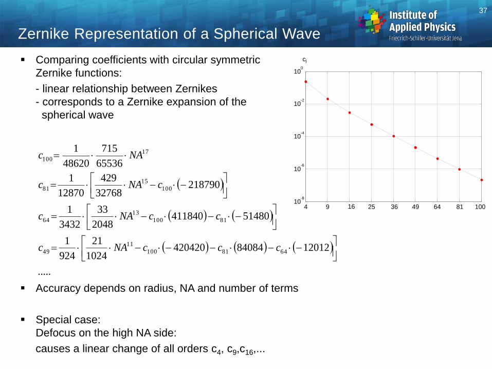
Zernike Representation of a Spherical Wave
Comparing coefficients with circular symmetric
Zernike functions:
- linear relationship between Zernikes
- corresponds to a Zernike expansion of the
spherical wave
Accuracy depends on radius, NA and number of terms
Special case:
Defocus on the high NA side:
causes a linear change of all orders c4, c9,c16,...
( )
( ) ( )
( ) ( ) ( )
.....
12012840844204201024
21
924
1
514804118402048
33
3432
1
21879032768
429
12870
1
65536
715
48620
1
6481100
11
49
81100
13
64
100
15
81
17
100
cccNAc
ccNAc
cNAc
NAc
4 9 16 25 36 49 64 81 10010
-8
10-6
10-4
10-2
100
cj
37

Zernike Representation of a Spherical Wave
Example:
Accuracy as a function of NA and
radius for 7 terms as a function of
position
NA = 0.8
z
r
NA = 0.9
NA = 0.6
-1 -0.5 0 0.5 110
-
10
10-8
10-6
10-4
10-2
38

Axial Intensity for Circular Symmetric Zernikes
Circular symmetric Zernikes:
- corresponds to a chirped radial phase grating
Increasing Talbot-effect along the axis causes a split of the axial intensity into
separated peaks
Effect grows with order and size of coefficient
The spreading of the side-lobes increases with the order
Corresponds to a multi-focus image
zRE
I(z)I(z)
-60 -40 -20 0 20 40 600
0.5
1
c = 0.3 n = 10
n = 14
n = 18
n = 24
n = 30
-60 -40 -20 0 20 40 600
0.5
1
c = 0.7 n = 10
n = 14
n = 18
n = 24
n = 30
zRE
I(z)
-60 -40 -20 0 20 40 600
0.5
1
c = 0.5 n = 10
n = 14
n = 18
n = 24
n = 30
39

Zernike Expansion of a Vignetted Pupil
Direct numerical (SVD optimization) expansion
of a vignetted amplitude in the pupil.
Apodization due to surface vignetting:
24% relative area.
Modelling of this profile by N Zernike
coefficients on a 128x128 grid
Errors in Apodization and corresponding Psf:
xM
rV
r
24%
Nzern Apod Rms
Apod PV Psf Rms Psf PV Psf Peak error [%]
36 0.1268 0.593 0.00113 0.0185 1.8
64 0.1083 0.568 6.4 10-4
0.0108 1.1
100 0.0962 0.531 3.8 10-4
0.0064 0.63
225 0.0765 0.512 6.2 10-5
8.5 10-4
0.13
40

Zernike Expansion of a Vignetted Pupil
N = 225N = 64N = 36 N = 100
Apodization
Error of
apodization
Error of
Psf
41

Zernike Expansion of a Vignetted Pupil
rms
50 100 150 200 25010
-5
10-4
10-3
10-2
10-1
100
Nzern
apodization
Psf
The improvement of the apodization itself grows slowly with the number of terms
The accuracy of the Psf in increased quite better
42

Zernike Expansion of a Vignetted Pupil
Cross section of the modelled apodization
amplitude A(y) and corresponding error
Poor convergence of the Zernike coefficients
cj
50 100 150 200 2500
0.1
0.2
0.3
0.4
0.5
-1 -0.5 0 0.5 1-0.4
-0.2
0
0.2
0.4
0.6
0.8
1
1.2
Apodization
A(y)
error A(y)
y
43

Performance Description by Zernike Expansion
Vector of cj
linear sequence with runnin g index
Sorting by symmetry
0 1 2 3 4 -1 -2 -3 -4
-0.2
-0.1
0
0.1
0.2
0.3
0.4
0.5
circular
symmetric
m = 0cos terms
m > 0
sin terms
m < 0
cj
m
44

Field Dependence of Zernike Coefficients
Usually the system quality changes with the field position
The natural behavior is
a decrease in quality from
the center to the edge
For spatial variant PSF
deconvolution or image
calculation applications,
a robust interpolation for
arbitrary field points is desirable
An interpolation of the PSF-intensity
distribution is nearly impossible
The individual Zernike coefficients vary
rather smoothly with the field location
An interpolation of the individual
Zernike coefficients therefore is quite
good -2
-1
0
1
2
3
4
0 0.1 0.2 0.3 0.4 0.5 0.6 0.7 0.8 0.9 1
cj in
relative
field
position
c4 defocus
c5 astigmatism
c8 coma
c9 spherical
c11
trefoil
c12
astigmatism 5. order
c15
coma 5. order
c16
spherical 5. order
x = 0 x = 20% x = 40% x = 60 % x = 80 % x = 100 %
45

Conventional usage of Zernike coefficients: - description of wave front in pupil - determines the PSF intensity in the reference plane
More general approach due to Braat (2005) according to an old idea of Zernike (1930) - expansion of the intensity I(x,y,z) in the image domain in all dimensions - lateral expansion into Zernikes - axial Taylor expansion with coefficients
cnm: classical Zernike coefficients
This gives an analytical representation of the volume distribution of intensity
Extended Zernike Approach
( )
++
+
++++
l
jlq
jp
l
l
lj
l
ljmjlmb pnm
lj
1
1
1
1
12)1(
22
mnq
mnp
+
( ) ( ) ( )
++
+
p
jl
jlmnm
lj
l
liz
mn
m
nmrl
rJbizemici
r
rJzrE
0
2
1
1
0,
1)(
2cos4)(2
2,,
46

Example: - intensity z-stack for coma - calculation with diffraction integral / extended Zernike approach - nearly perfect result without differences
Extended Zernike Approach
z = -1.5 -1.0 -0.5 0 0.5 1.0 1.5
ccoma = 0.05
diffraction
integral
extended
Nijboer-
Zernike
47

Extended Zernike Accuracy
Problems with extended Zernikes: 1. circular coordinates 2. no apodization 3. truncation of expansion critical, in particular along z finite range of convergence
Example calculation: accuracy as a function of growing coefficients for fixed number of terms
0
0.1
0.2
0.3
0.4
0.5
0 0.2 0.4 0.6 0.8 1
Irms
cj
defocus
astigmatism
coma
spherical
defocus
astigmatism
coma
spherical
0 0.2 0.4 0.6 0.8 1
correlation
cj0.5
0.6
0.7
0.8
0.9
1
48