Embed Size (px)
Citation preview
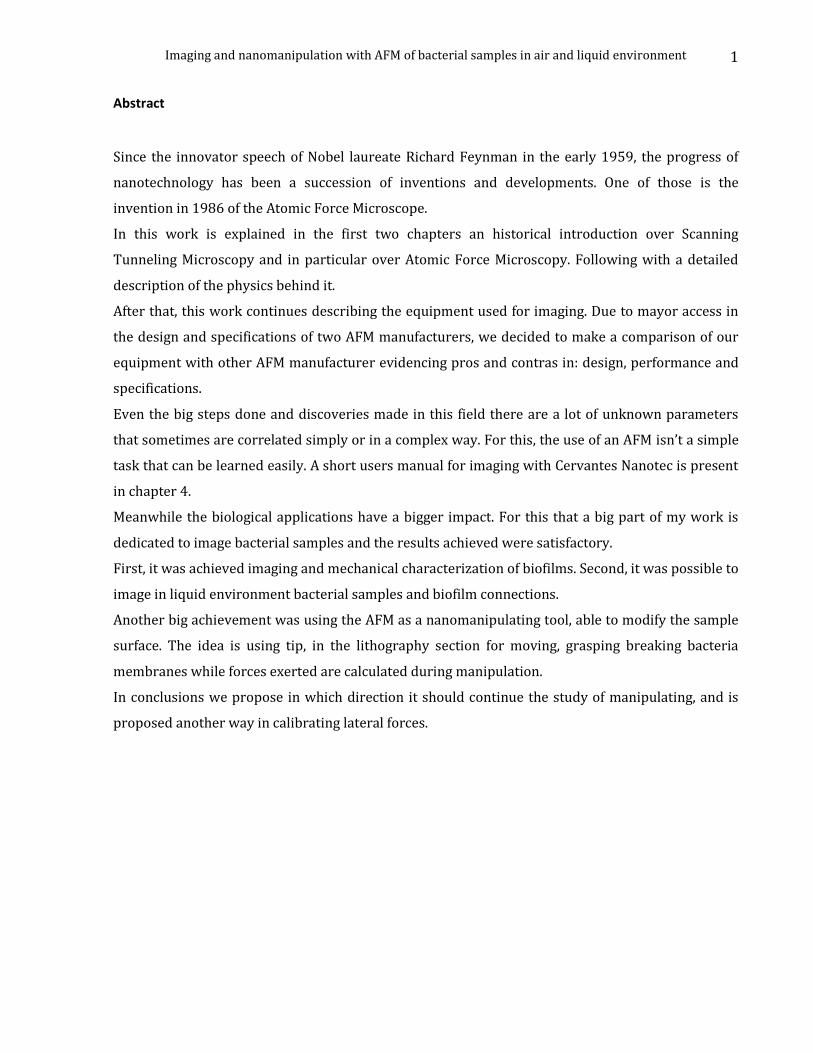
Imaging and nanomanipulation with AFM of bacterial samples in air and liquid environment
1
Abstract
Since the innovator speech of Nobel laureate Richard Feynman in the early 1959, the progress of
nanotechnology has been a succession of inventions and developments. One of those is the
invention in 1986 of the Atomic Force Microscope.
In this work is explained in the first two chapters an historical introduction over Scanning
Tunneling Microscopy and in particular over Atomic Force Microscopy. Following with a detailed
description of the physics behind it.
After that, this work continues describing the equipment used for imaging. Due to mayor access in
the design and specifications of two AFM manufacturers, we decided to make a comparison of our
equipment with other AFM manufacturer evidencing pros and contras in: design, performance and
specifications.
Even the big steps done and discoveries made in this field there are a lot of unknown parameters
that sometimes are correlated simply or in a complex way. For this, the use of an AFM isn’t a simple
task that can be learned easily. A short users manual for imaging with Cervantes Nanotec is present
in chapter 4.
Meanwhile the biological applications have a bigger impact. For this that a big part of my work is
dedicated to image bacterial samples and the results achieved were satisfactory.
First, it was achieved imaging and mechanical characterization of biofilms. Second, it was possible to
image in liquid environment bacterial samples and biofilm connections.
Another big achievement was using the AFM as a nanomanipulating tool, able to modify the sample
surface. The idea is using tip, in the lithography section for moving, grasping breaking bacteria
membranes while forces exerted are calculated during manipulation.
In conclusions we propose in which direction it should continue the study of manipulating, and is
proposed another way in calibrating lateral forces.

Imaging and nanomanipulation with AFM of bacterial samples in air and liquid environment
2
Resumen
Desde el discurso innovador del premio Nobel Richard Feynman en los principios de 1959, el
progreso de la nanotecnología ha sido una sucesión de invenciones y desarrollos. Uno de estas
invenciones es el Microscopio a Fuerzas Atómicas (AFM) en el 1986 por Binning.
En éste trabajo se explica en los primeros dos capítulos una breve historia sobre las Scanning
Tunneling Microscopy y más en particular sobre el AFM, seguido de una descripción detallada de las
leyes físicas que están detrás de esta invención.
Después de esto, se continua con una descripción del equipo usado y debido a mayor acceso en el
diseño y las especificaciones de dos productores de AFM, se ha decidido hacer una comparación
entre los dos evidenciando los pros y los contras sobre el diseño, actuación y especificaciones.
Aunque la grande invención, hay muchos parámetros que aún no se sabe como están relacionados
entre ellos, algunos sencillamente y otros en manera más complicada. Por esto que se ha pensado de
hacer un pequeño manual de uso para los principiantes, que es el capítulo 4.
Mientras que las aplicaciones biológicas del AFM tienen un mayor impacto debido a la cantidad de
información que se puede sacar. En el capítulo 5 se han conseguido dos resultados muy buenos.
Primero, se ha hecho posible hacer imágenes y caracterizar mecánicamente biofilms. Segundo, se ha
conseguido hacer imágenes en ambiente liquido de biofilms.
Otro gran resultado es el utilice del AFM como una herramienta para la manipulación de superficies
y membranas. Básicamente ha sido usada la punta de AFM como una nano-herramienta capaz de
mover, rascar y romper membranas de bacterias.
En conclusión, proponemos unas futuras direcciones de estudio, y una innovadora manera de
calibrar la fuerza lateral.
Imaging and nanomanipulation with AFM of bacterial samples in air and liquid environment
3
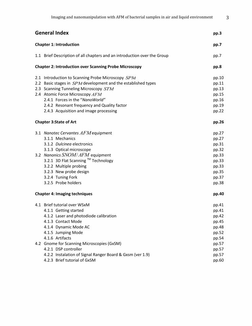
General Index pp.3
Chapter 1: Introduction pp.7 1.1 Brief Description of all chapters and an introduction over the Group pp.7 Chapter 2: Introduction over Scanning Probe Microscopy pp.8 2.1 Introduction to Scanning Probe Microscopy SPM pp.10 2.2 Basic stages in SPM development and the established types pp.11 2.3 Scanning Tunneling Microscopy STM pp.13 2.4 Atomic Force Microscopy AFM pp.15
2.4.1 Forces in the “NanoWorld” pp.16 2.4.2 Resonant frequency and Quality factor pp.19 2.4.3 Acquisition and image processing pp.22
Chapter 3:State of Art pp.26 3.1 Nanotec Cervantes AFM equipment pp.27
3.1.1 Mechanics pp.27 3.1.2 Dulcinea electronics pp.31 3.1.3 Optical microscope pp.32
3.2 Nanonics SNOM /AFM equipment pp.33 3.2.1 3D Flat Scanning TM Technology pp.33 3.2.2 Multiple probing pp.33 3.2.3 New probe design pp.35 3.2.4 Tuning Fork pp.37 3.2.5 Probe holders pp.38
Chapter 4: Imaging techniques pp.40 4.1 Brief tutorial over WSxM pp.41
4.1.1 Getting started pp.41 4.1.2 Laser and photodiode calibration pp.42 4.1.3 Contact Mode pp.45 4.1.4 Dynamic Mode AC pp.48 4.1.5 Jumping Mode pp.52 4.1.6 Artifacts pp.54
4.2 Gnome for Scanning Microscopies (GxSM) pp.57 4.2.1 DSP controller pp.57 4.2.2 Instalation of Signal Ranger Board & Gxsm (ver 1.9) pp.57 4.2.3 Brief tutorial of GxSM pp.60
Imaging and nanomanipulation with AFM of bacterial samples in air and liquid environment
4
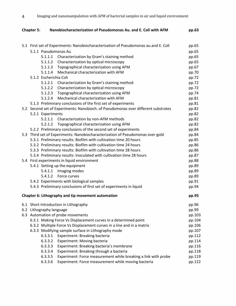
Chapter 5: Nanobiocharacterization of Pseudomonas Au. and E. Coli with AFM pp.63
5.1 First set of Experiments: Nanobiocharacterization of Pseudomonas au.and E. Coli pp.65
5.1.1 Pseudomonas Au pp.65 5.1.1.1 Characterization by Gram’s staining method pp.65 5.1.1.2 Characterization by optical microscopy pp.65 5.1.1.3 Topographical characterization using AFM pp.67 5.1.1.4 Mechanical characterization with AFM pp.70
5.1.2 Escherichia Coli pp.72 5.1.2.1 Characterization by Gram’s staining method pp.72 5.1.2.2 Characterization by optical microscopy pp.72 5.1.2.3 Topographical characterization using AFM pp.74 5.1.2.4 Mechanical characterization with AFM pp.81
5.1.3 Preliminary conclusions of the first set of experiments pp.81 5.2 Second set of Experiments: Nanobioch. of Pseudomonas over different substrates pp.82
5.2.1 Experiments pp.82 5.2.1.1 Characterization by non-AFM methods pp.82 5.2.1.2 Topographical characterization using AFM pp.82
5.2.2 Preliminary conclusions of the second set of experiments pp.84 5.3 Third set of Experiments: Nanobiocharacterization of Pseudomonas over gold pp.84
5.3.1 Preliminary results: Biofilm with cultivation time 20 hours pp.85 5.3.2 Preliminary results: Biofilm with cultivation time 24 hours pp.86 5.3.3 Preliminary results: Biofilm with cultivation time 28 hours pp.86 5.3.4 Preliminary results: Inoculated with cultivation time 28 hours pp.87
5.4 First experiments in liquid environment pp.88 5.4.1 Setting up the equipment pp.89
5.4.1.1 Imaging modes pp.89 5.4.1.2 Force curves pp.89
5.4.2 Experiments with biological samples pp.91 5.4.3 Preliminary conclusions of first set of experiments in liquid pp.94
Chapter 6: Lithography and tip movement automation pp.95
6.1 Short Introduction in Lithography pp.96 6.2 Lithography language pp.99 6.3 Automation of probe movements pp.103
6.3.1 Making Force Vs Displacement curves in a determined point pp.104 6.3.2 Multiple Force Vs Displacement curves in a line and in a matrix pp.106 6.3.3 Modifying sample surface in Lithography mode pp.107
6.3.3.1 Experiment: Breaking bacteria pp.112 6.3.3.2 Experiment: Moving bacteria pp.114 6.3.3.3 Experiment: Breaking bacteria’s membrane pp.116 6.3.3.4 Experiment: Breaking through a bacteria pp.118 6.3.3.5 Experiment: Force measurement while breaking a link with probe pp.119 6.3.3.6 Experiment: Force measurement while moving bacteria pp.122
Imaging and nanomanipulation with AFM of bacterial samples in air and liquid environment
5
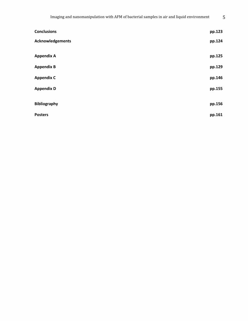
Conclusions pp.123
Acknowledgements pp.124
Appendix A pp.125 Appendix B pp.129 Appendix C pp.146 Appendix D pp.155
Bibliography pp.156 Posters pp.161
Imaging and nanomanipulation with AFM of bacterial samples in air and liquid environment
6
Imaging and nanomanipulation with AFM of bacterial samples in air and liquid environment
7
Chapter 1: Introduction
On the evening of December 29, 1959, Nobel Laureate Richard Feynman [1] delivered a visionary
7000 word after-dinner talk to a meeting of the American Physical Society at the California Institute
of Technology. It was entitled “There’s Plenty of Room at the Bottom”. It was the defining moment
for nanoscience and the future of nanotechnology.
“I would like to describe a field in which little has been done, but in which an enormous amount can be
done in principle…What I want to talk about is the problem of manipulating and controlling things on
a small scale.” Richard Feynman.
In the course of his lecture, Feynman made this prediction: “In the year 2000, when they look back
at this age, they will wonder why it was not until the year 1960 that anybody began seriously to
move in this direction.” But there’s a simple reason people didn’t immediately begin working at
the nanoscale. They didn’t have the tools. The scanning tunneling microscope and the atomic force
microscope were the two most important tools at the beginning of the nanoscale revolution, but
now there’s an expanding toolkit of devices used to observe, measure, and manipulate nanoscale
structures. And as we learn more about the nanoscale world, we’ll be able to make even better tools.
We had to wait till 1981 that Nobel Laureate Binning, invents Scanning Tunneling Microscope; a
modern tool for studying the morphology and the local properties of the solid body surfaces with a
high spatial resolution.
In chapter 2 we are going to speak about the physics that stays behind the SPM and more in
particular of Atomic Force Microscope. Through some simple passages we will discover the forces
that stays behind and some simplified models of AFM feedback and cantilever motion equations.
Instead in chapter 3 we discuss the state of art in manufacturing AFM. And more in
particular on Nanotec Electrónica and Nanonics. The first one is the producer of our own microscope
and the second one are the manufacturers of Multiprobe 4000 explained more in detail further.
Chapter 4 is a short AFM manual for beginners. Briefly introducing WSxM (software
controlling AFM electronics), we describe how to use the microscope in the three main modes:
contact (DC), dynamic (AC) and Jumping (JM). The equivalent open source code is named GxSM, and
in this chapter we describe another open source solution to SPM.
Chapter 5 includes a good biological study over two main types of bacteria: Pseudomonas
aeruginosa and Escherichia Coli as among the most popular and of relevant study interest. We pass
through an optical phase, later a topographical and mechanical characterization of their
Imaging and nanomanipulation with AFM of bacterial samples in air and liquid environment
8
membranes. The main interest in characterizing these two groups of bacteria is: their ability to
survive in extreme conditions (good for our experiments in air), their ability to form biofilms
presenting resistance to antibiotics (as different studies have been observing).
We conclude this chapter with two main achievings:
1. Mechanical and topographical characterization of biofilm over Pseudomonas and E.Coli.
2. Topographical characterization of biofilms in liquid environment.
Chapter 6 gives another optics of AFM. Till now we have been customized to see at an AFM
as a proximity microscope; good for discovering rigid body surface properties. But here we use AFM
probes for manipulating surfaces, moving bacteria, breaking links between them and more
important is the ability to record forces the probe is experimenting during manipulation.
In this chapter are exposed some simple manipulations like: grasping surface, moving bacteria,
breaking membranes, calculating forces exerted over the probe. Some simple tasks but really
important regarding information we get. Till now, only few research groups have been able to
measure forces exerted over bacterial membranes using AFM.
“Are you having trouble imagining a nanometer? If you are, don't feel bad. You aren't alone.”
Imaging and nanomanipulation with AFM of bacterial samples in air and liquid environment
9
Chapter 2: Introduction over Scanning Probe Microscopy pp.9 Chapter Index 2.1 Introduction to Scanning Probe Microscopy SPM pp.10 2.2 Basic stages in SPM development and the established types pp.11 2.3 Scanning Tunneling Microscopy STM pp.13 2.4 Atomic Force Microscopy AFM pp.15
2.4.1 Forces in the “NanoWorld” pp.16 2.4.2 Resonant frequency and Quality factor pp.19 2.4.3 Acquisition and image processing pp.22
Imaging and nanomanipulation with AFM of bacterial samples in air and liquid environment
10
2.1 Introduction to SPM
The concept of the atom has been around in one form or another since the ancient Greeks. Yet at the
beginning of the twentieth century, there were still some scientists who doubted the atom’s
existence. To them, an atom was simply a useful fiction. It took Albert Einstein, in a 1905 paper, to
explain the indirect evidence for the existence of atoms and to show that the sizes of atoms and
molecules could be determined. Nonetheless, scientists doubted that we’d ever be able to observe
an atom, or anything else smaller than a few hundred nanometers, because of diffraction limits
imposed by the nature of the light, until (SPM)invention in 1981.
The Scanning Probe Microscopy (SPM) is one of the powerful modern research techniques that
allow investigating the morphology and the local properties of the solid body surface with high
spatial resolution. During last decades the scanning probe microscopy has turned from an exotic
technique accessible only to a limited number of research groups, to a widespread and successfully
used research tool of surface properties. Currently, practically every research in the field of surface
physics and thin-film technologies applies the SPM techniques. The scanning probe microscopy has
formed also a basis for development of new methods in nanotechnology, i.e. the technology of
creation of structures at nanometric scales.
The Scanning Tunneling Microscope (STM) is the first in the probe microscopes family; invented in
1981 by the Swiss scientists G. Binnig and H. Rohrer [2][3]. In their works they have shown, that this
is a quite simple and rather effective way to study a surface with spatial resolution down to atomic
one. Their technique was fully acknowledged after visualization of the atomic structure of the
surface of some materials and, particularly, the reconstructed surface of silicon. In 1986, G. Binnig
and H. Rohrer were awarded the Nobel Prize in physics for invention of the tunneling microscope.
After the tunneling microscope creation, Atomic Force Microscope (AFM ) , Magnetic Force
Microscope (MFM) , Electric Force Microscope (EFM ), Scanning Near-field Optical Microscope
(SNOM) and many other devices having similar working principles and named as scanning probe
microscopes have been created within a short period of time.
Working principle: By using specially prepared tips in the form of needles is performed the analysis
of a surface and of its local properties. The size of the working part of such tips (the apex) is about
ten nanometers. The usual tip - surface distance in probe microscopes is about 0.1 – 10 nanometers.
Imaging and nanomanipulation with AFM of bacterial samples in air and liquid environment
11
Various types of interaction of the tip with the surface are exploited in different types of probe
microscopes. For example the tunnel microscope is based on the phenomenon of a tunneling
current between a metal needle and a conducting sample.
2.2 Basic stages in SPM development and the established types
Since 1981, there have been developed several techniques and here bellow we are going to list the
most important ones in a chronologic order.
1981 - Scanning tunneling microscope. G. Binnig, H. Rohrer.
Atomic resolution images of conducting surfaces.
1982 - Scanning near-field optical microscope. D. W. Pohl.
Resolution of 50 nanometers in optical images.
1984 - Scanning capacitive microscope. J. R. Matey, J. Blanc.
500 nm (lateral resolution) images of capacitance variation.
1985 - Scanning thermal microscope. C. C. Williams, H. K. Wickramasinghe.
Resolution of 50 nm in thermal images.
1986 - Atomic-force microscope. G. Binnig, C. F. Quate, Ch. Gerber.
Atomic resolution on non-conducting (and conducting) samples.
1987 - Magnetic-force microscope. Y. Martin, H. K. Wickramasinghe.
Resolution of 100 nanometers in magnetic images.
″Frictional″force microscope. C. M. Mate, G. M. McClelland, S. Chiang.
Atomic-scale images of lateral (″frictional″) forces.
Electric force microscope. Y. Martin, D. W. Abraham, H. K. Wickramasinghe.
Detecting of single charges on a sample surface.
Inelastic tunneling STM spectroscopy. D. P. E. Smith, D. Kirk, C. F. Quare.
Detection of phonon spectra of molecules in STM.
Laser driven STM. L. Arnold, W. Krieger, H. Walther.
Imaging by non-linear mixing of optical waves in STM.
1988 - Ballistic electron emission microscope. W. J. Kaiser.
Schottky barriers investigation with nanometer resolution.
Inverse photoemission microscope. J. H. Coombs, J. K. Gimzewski, B. Reihl et al
Detection of luminescence spectra on nanometer scales.
1989 – Near-field acoustic microscope. K. Takata, T. Hasegawa, S. Hosaka, S. Hosoki.
Imaging and nanomanipulation with AFM of bacterial samples in air and liquid environment
12
Low-frequency acoustic measurements with the resolution of 10 nm.
Scanning noise microscope. R. Moller A. Esslinger, B. Koslowski.
Detection of tunnel current without voltage bias.
Scanning spin - precession microscope. Y. Manassen, R. Hamers, J. Demuth
Visualization of spin in a paramagnetics with 1 nm resolution.
Scanning ion-conductance microscope. P. Hansma, B. Drake, O. Marti, S. Gould
Imaging in electrolyte with 500 nm resolution.
Scanning electrochemical microscope. O. E. Husser, D. H. Craston, A. J. Bard.
1990 - Scanning chemical potential microscope. C. C. Williams, H. K. Wickramasinghe.
Atomic scale images of chemical potential variation.
Photovoltage STM. R. J. Hamers, K. Markert.
Photovoltage images on nanometer scale.
1991 - Kelvin probe force microscope.N. Nonnenmacher, M. P. O'Boyle
1994 – Apertureless near-field optical microscope.
F. Zenhausern, M. P. O'Boyle, H. K. Wickramasinghe.
Optical microscopy with 1 nm resolution.
Many other microscopy techniques have been developed based upon SPM. The followings are the
established types:
(AFM ) Atomic force microscopy consists of a micro scale cantilever with a sharp tip at its
end that is used to scan the specimen surface.
(BEEM) Ballistic electron emission microscopy, studies ballistic electron transport through
variety of materials and material interfaces.
(EFM ) Electrostatic force microscopy plots the locally charged domains of the sample
surface; similar to how MFMplots the magnetic domains of the sample surface.
(ESTM)Electrochemical scanning tunneling microscopy, studies the structure of the
electrochemical processes at molecular or atomic level.
(FMM) Force modulation microscopy, is an extension of AFM imaging that includes
characterization of a sample's mechanical properties. Like LFMand MFM,FMM allows
simultaneous acquisition of both topographic and material-properties data.
(KPFM)Kelvin probe force microscopy is based on the measurement of the electrostatic
forces between the small conducting AFM tip and the sample.
Imaging and nanomanipulation with AFM of bacterial samples in air and liquid environment
13
(MFM) Magnetic force microscopy, measures magnetic force between the tip and sample.
(MRFM)Magnetic resonance force microscopy combines the ideas of magnetic resonance
imaging (MRI) and AFM.
(NSOM)Near-Field scanning optical microscopy or (SNOM) , breaks the far field resolution
limit by exploiting the properties of evanescent waves.
(PDM)Phase detection microscopy, is another technique that can be used to map
variations in surface properties such as elasticity, adhesion, and friction.
(PSTM)Photon scanning tunneling microscopy.
(PTMS)Photothermal microscopy is derived from two parent instrumental techniques:
infrared spectroscopy and AFM.
(SECM)Scanning electrochemical microscopy.
(SCM)Scanning capacitance microscopy, images spatial variations in capacitance by
inducing a voltage between the tip and the sample. Characterizes sample surface using
information obtained from electrostatic capacitance changes between surface and probe.
(SGM)Scanning gate microscopy, with an electrically conductive tip used as a movable gate
that couples with a capacitance the sample and probes electrical transport.
(SICM)Scanning ion-conductance microscopy, maps local ion currents above the surface.
(SPSM)Spin polarized microscopy.
(SThM)Scanning thermal microscopy, measures sample’s surface thermal conductivity.
(STM) Scanning tunneling microscopy studies local electronic structure of a sample.
(SVM)Scanning voltage microscopy is based in obtaining an electric potential map of the
raster surface with the use of conductive probes.
(SHPM) Scanning Hall probe microscopy helps creating a magnetic induction map by
coupling STM with a semiconductor Hall sensor.
2.3 Scanning Tunneling Microscopy
Historically, the first microscope in the family of probe microscopes is the scanning tunneling
microscope. The working principle of STM is based on the phenomenon of electrons tunneling
through a narrow potential barrier between a metal tip and a conducting sample in an external
electric field.
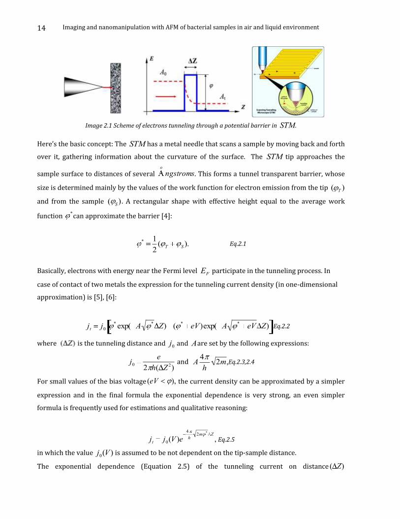
Imaging and nanomanipulation with AFM of bacterial samples in air and liquid environment
14
Image 2.1 Scheme of electrons tunneling through a potential barrier in STM.
Here’s the basic concept: The STM has a metal needle that scans a sample by moving back and forth
over it, gathering information about the curvature of the surface. The STM tip approaches the
sample surface to distances of several o
ngstroms. This forms a tunnel transparent barrier, whose
size is determined mainly by the values of the work function for electron emission from the tip ( T )
and from the sample ( S ) . A rectangular shape with effective height equal to the average work
function *can approximate the barrier [4]:
* 1
2( T S ). Eq.2.1
Basically, electrons with energy near the Fermi level EF participate in the tunneling process. In
case of contact of two metals the expression for the tunneling current density (in one-dimensional
approximation) is [5], [6]:
jt j0
* exp( A * Z) ( * eV)exp( A * eV Z) ,Eq.2.2
where is the tunneling distance and j0 and Aare set by the following expressions:
j0
e
2 h( Z 2) and A
4
h2m,Eq.2.3,2.4
For small values of the bias voltage (eV ), the current density can be approximated by a simpler
expression and in the final formula the exponential dependence is very strong, an even simpler
formula is frequently used for estimations and qualitative reasoning:
jt j0(V )e4
h2m * Z
, Eq.2.5
in which the value j0(V ) is assumed to be not dependent on the tip-sample distance.
The exponential dependence (Equation 2.5) of the tunneling current on distance ( Z)
Imaging and nanomanipulation with AFM of bacterial samples in air and liquid environment
15
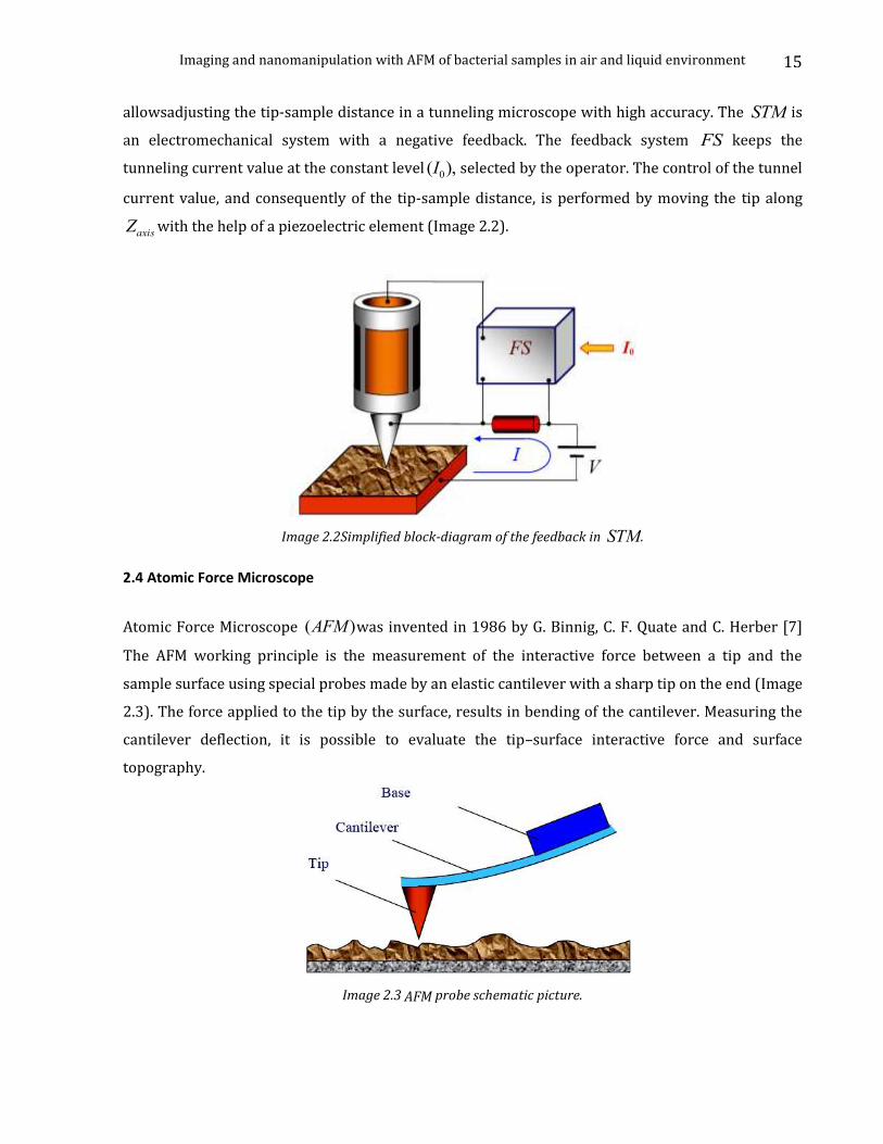
allowsadjusting the tip-sample distance in a tunneling microscope with high accuracy. The STM is
an electromechanical system with a negative feedback. The feedback system FS keeps the
tunneling current value at the constant level (I0), selected by the operator. The control of the tunnel
current value, and consequently of the tip-sample distance, is performed by moving the tip along
Zaxis with the help of a piezoelectric element (Image 2.2).
Image 2.2Simplified block-diagram of the feedback in STM.
2.4 Atomic Force Microscope
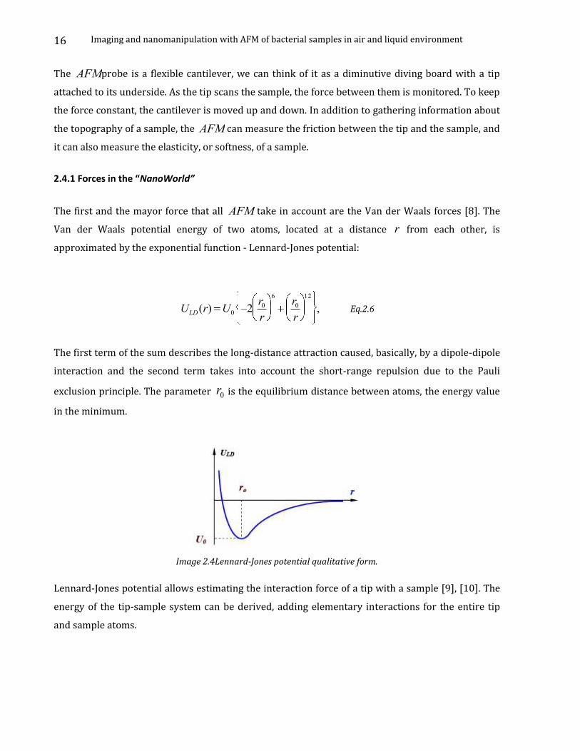
Atomic Force Microscope (AFM )was invented in 1986 by G. Binnig, C. F. Quate and C. Herber [7]
The AFM working principle is the measurement of the interactive force between a tip and the
sample surface using special probes made by an elastic cantilever with a sharp tip on the end (Image
2.3). The force applied to the tip by the surface, results in bending of the cantilever. Measuring the
cantilever deflection, it is possible to evaluate the tip–surface interactive force and surface
topography.
Image 2.3 AFM probe schematic picture.
Imaging and nanomanipulation with AFM of bacterial samples in air and liquid environment
16
The AFMprobe is a flexible cantilever, we can think of it as a diminutive diving board with a tip
attached to its underside. As the tip scans the sample, the force between them is monitored. To keep
the force constant, the cantilever is moved up and down. In addition to gathering information about
the topography of a sample, the AFM can measure the friction between the tip and the sample, and
it can also measure the elasticity, or softness, of a sample.
2.4.1 Forces in the “NanoWorld”
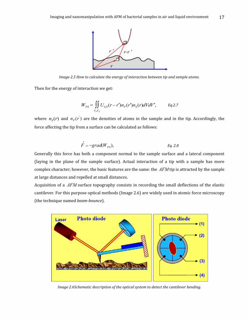
The first and the mayor force that all AFM take in account are the Van der Waals forces [8]. The
Van der Waals potential energy of two atoms, located at a distance r from each other, is
approximated by the exponential function - Lennard-Jones potential:
ULD(r) U0 2r0
r
6r0
r
12
, Eq.2.6
The first term of the sum describes the long-distance attraction caused, basically, by a dipole-dipole
interaction and the second term takes into account the short-range repulsion due to the Pauli
exclusion principle. The parameter r0 is the equilibrium distance between atoms, the energy value
in the minimum.
Image 2.4Lennard-Jones potential qualitative form.
Lennard-Jones potential allows estimating the interaction force of a tip with a sample [9], [10]. The
energy of the tip-sample system can be derived, adding elementary interactions for the entire tip
and sample atoms.
Imaging and nanomanipulation with AFM of bacterial samples in air and liquid environment
17
Image 2.5 How to calculate the energy of interaction between tip and sample atoms.
Then for the energy of interaction we get:
WPS ULD(r r )nP (r )nS (r)VPVS
dVdV , Eq.2.7
where nS(r) and nP (r') are the densities of atoms in the sample and in the tip. Accordingly, the
force affecting the tip from a surface can be calculated as follows:
F grad(WPS), Eq. 2.8
Generally this force has both a component normal to the sample surface and a lateral component
(laying in the plane of the sample surface). Actual interaction of a tip with a sample has more
complex character; however, the basic features are the same: the AFM tip is attracted by the sample
at large distances and repelled at small distances.
Acquisition of a AFM surface topography consists in recording the small deflections of the elastic
cantilever. For this purpose optical methods (Image 2.6) are widely used in atomic force microscopy
(the technique named beam-bounce).
Image 2.6Schematic description of the optical system to detect the cantilever bending.
Imaging and nanomanipulation with AFM of bacterial samples in air and liquid environment
18
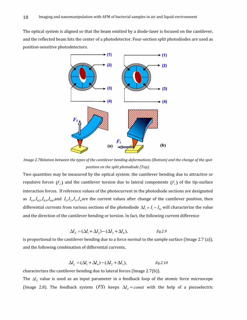
The optical system is aligned so that the beam emitted by a diode-laser is focused on the cantilever,
and the reflected beam hits the center of a photodetector. Four-section split photodiodes are used as
position-sensitive photodetectors.
Image 2.7Relation between the types of the cantilever bending deformations (Bottom) and the change of the spot
position on the split photodiode (Top).
Two quantities may be measured by the optical system: the cantilever bending due to attractive or
repulsive forces FZ and the cantilever torsion due to lateral components FL
of the tip-surface
interaction forces. If reference values of the photocurrent in the photodiode sections are designated
as I01,I02,I03,I04,and I1,I2,I3,I4are the current values after change of the cantilever position, then
differential currents from various sections of the photodiode Ii Ii I0i will characterize the value
and the direction of the cantilever bending or torsion. In fact, the following current difference
IZ ( I1 I2) ( I3 I4), Eq.2.9
is proportional to the cantilever bending due to a force normal to the sample surface (Image 2.7 (a)),
and the following combination of differential currents,
IL ( I1 I4) ( I2 I3), Eq.2.10
characterizes the cantilever bending due to lateral forces (Image 2.7(b)).
The IZ value is used as an input parameter in a feedback loop of the atomic force microscope
(Image 2.8). The feedback system (FS) keeps IZ const with the help of a piezoelectric
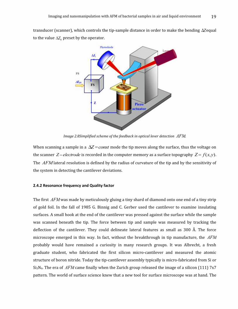
Imaging and nanomanipulation with AFM of bacterial samples in air and liquid environment
19
transducer (scanner), which controls the tip-sample distance in order to make the bending Zequal
to the value Z0 preset by the operator.
Image 2.8Simplified scheme of the feedback in optical lever detection AFM.
When scanning a sample in a Z const mode the tip moves along the surface, thus the voltage on
the scanner Z electrode is recorded in the computer memory as a surface topography Z f (x,y) .
The AFM lateral resolution is defined by the radius of curvature of the tip and by the sensitivity of
the system in detecting the cantilever deviations.
2.4.2 Resonance frequency and Quality factor
The first AFM was made by meticulously gluing a tiny shard of diamond onto one end of a tiny strip
of gold foil. In the fall of 1985 G. Binnig and C. Gerber used the cantilever to examine insulating
surfaces. A small hook at the end of the cantilever was pressed against the surface while the sample
was scanned beneath the tip. The force between tip and sample was measured by tracking the
deflection of the cantilever. They could delineate lateral features as small as 300 Å. The force
microscope emerged in this way. In fact, without the breakthrough in tip manufacture, the AFM
probably would have remained a curiosity in many research groups. It was Albrecht, a fresh
graduate student, who fabricated the first silicon micro-cantilever and measured the atomic
structure of boron nitride. Today the tip-cantilever assembly typically is micro-fabricated from Si or
Si3N4. The era of AFM came finally when the Zurich group released the image of a silicon (111) 7x7
pattern. The world of surface science knew that a new tool for surface microscope was at hand. The

Imaging and nanomanipulation with AFM of bacterial samples in air and liquid environment
20
interaction force F of a tip with the surface can be estimated from the Hooke law:
F k Z, Eq. 2.11
where k is the cantilever elastic constant; Zis the tip displacement corresponding to the bending
produced by the interaction with the surface. The k values vary in the range 10 3 10N /m
depending on the cantilever material and geometry. The cantilever resonant frequency is important
during AFM operation in oscillating modes. Self-frequencies of cantilever oscillations are
determined by the following formula (see, for example, [11]):
rii
l2
EJ
S, Eq.2.12
where lis the cantilever length; E the Young’s modulus; J the inertia moment of the cantilever
cross-section; the material density; Sthe cross section; a numerical coefficient (in the range
1 100), depending on the oscillations mode.
Image 2.9Main cantilever oscillations modes.
Frequencies of the main modes are usually in the 10 1000kHz range. The quality factor Q of
cantilevers mainly depends on the media in which they operate.
Typical Q values are represented in Table 2.1.
In Vacuum In Air In Liquid
Q 103 104 300 500 10 100
Table 2.1 Q values achieved with the beam bounce method in three medias.
The exact description of the AFM cantilever oscillations is a complex mathematical task. However,
the basic features of the processes occurring during interaction of an oscillating cantilever with a
surface can be understood on the basis of elementary models, in particular, using the approximation
of a localized mass model [12]. Let us approximate the cantilever as an elastic mass less beam (with
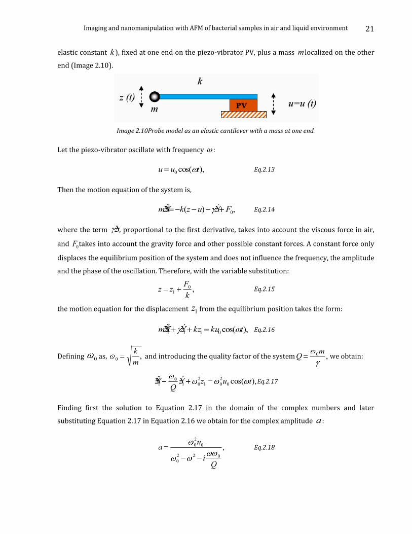
Imaging and nanomanipulation with AFM of bacterial samples in air and liquid environment
21
elastic constant k ), fixed at one end on the piezo-vibrator PV, plus a mass m localized on the other
end (Image 2.10).
Image 2.10Probe model as an elastic cantilever with a mass at one end.
Let the piezo-vibrator oscillate with frequency :
u u0 cos( t), Eq.2.13
Then the motion equation of the system is,
mÝ Ý z k(z u) Ý z F0, Eq.2.14
where the term Ý z , proportional to the first derivative, takes into account the viscous force in air,
and F0takes into account the gravity force and other possible constant forces. A constant force only
displaces the equilibrium position of the system and does not influence the frequency, the amplitude
and the phase of the oscillation. Therefore, with the variable substitution:
z z1
F0
k, Eq.2.15
the motion equation for the displacement z1 from the equilibrium position takes the form:
mÝ Ý z 1 Ý z 1 kz1 ku0 cos( t), Eq.2.16
Defining 0 as, 0
k
m, and introducing the quality factor of the system Q 0m , we obtain:
Ý Ý z 10
QÝ z 1 0
2z1 0
2u0 cos( t),Eq.2.17
Finding first the solution to Equation 2.17 in the domain of the complex numbers and later
substituting Equation 2.17 in Equation 2.16 we obtain for the complex amplitude a :
a 0
2u0
0
2 2 i 0
Q
, Eq.2.18
Imaging and nanomanipulation with AFM of bacterial samples in air and liquid environment
22
The module of ais the forced oscillations amplitude A( ) :
A( )u0 0
2
( 0
2 2)2
2
0
2
Q2
, Eq.2.19
The phase of the complex amplitude ais the phase difference ( ) between the system oscillation
and the forcing term u u0 cos( t) :
( ) arctg 0
Q( 0
2 2), Eq.2.20
From equation 2.19 it follows, that the tip oscillation amplitude A( 0) Qu0, at the frequency 0,
is proportional to the quality factor. Besides that, the presence of dissipation ( 0, i.e. Q ) in
the system results in a decrease of the resonant frequency of the cantilever oscillations. Indeed,
differentiating the radicand with respect to 2in equation 2.19 and equating the derivative to zero,
we obtain for the resonant frequency rd :
rd
2
0
2 11
2Q2, Eq.2.21
Equation 2.21 shows the real dependency of the resonant frequency from the Quality factor, where
high Q values imply rd 0 . In this way there are needed smaller forces for achieving resonant
frequencies. As several works show [13], [14], is important of increase system’s quality factor as it
avoids sample deterioration. In future works there are a lot of groups which intent to increase the
quality factor by hardware (by using two or more Lock-in amplifiers, MAC mode of Agilent
Technologies [15]) for augmenting Q .
2.4.3 Acquisition and image processing
Scanning a surface with AFM is like moving an electronic beam on the screen in the cathode ray tube
of a TV. The tip goes along a (row) first in forward, and then in the reverse direction (horizontal
scanning), then passes to the next line (frame scanning). Tip movement is done in small steps by the
scanner that is driven by a saw tooth voltage produced by digital-to-analog converters. The surface
topographic information can be stored during forward/backward pass. (Image 2.11)
The information collected by the scanning probe microscope, is stored as a two-dimensional file of
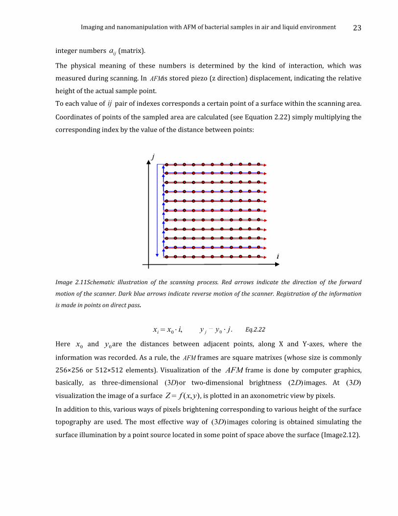
Imaging and nanomanipulation with AFM of bacterial samples in air and liquid environment
23
integer numbers aij (matrix).
The physical meaning of these numbers is determined by the kind of interaction, which was
measured during scanning. In AFMis stored piezo (z direction) displacement, indicating the relative
height of the actual sample point.
To each value of ij pair of indexes corresponds a certain point of a surface within the scanning area.
Coordinates of points of the sampled area are calculated (see Equation 2.22) simply multiplying the
corresponding index by the value of the distance between points:
Image 2.11Schematic illustration of the scanning process. Red arrows indicate the direction of the forward
motion of the scanner. Dark blue arrows indicate reverse motion of the scanner. Registration of the information
is made in points on direct pass.
xi x0 i, y j y0 j. Eq.2.22
Here x0 and y0are the distances between adjacent points, along X and Y-axes, where the
information was recorded. As a rule, the AFM frames are square matrixes (whose size is commonly
256×256 or 512×512 elements). Visualization of the AFM frame is done by computer graphics,
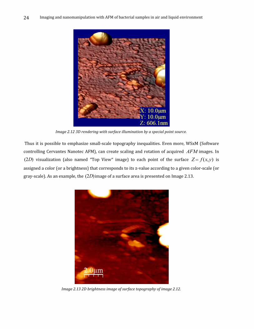
basically, as three-dimensional (3D)or two-dimensional brightness (2D) images. At (3D)
visualization the image of a surface Z f (x,y), is plotted in an axonometric view by pixels.
In addition to this, various ways of pixels brightening corresponding to various height of the surface
topography are used. The most effective way of (3D) images coloring is obtained simulating the
surface illumination by a point source located in some point of space above the surface (Image2.12).
Imaging and nanomanipulation with AFM of bacterial samples in air and liquid environment
24
Image 2.12 3D rendering with surface illumination by a special point source.
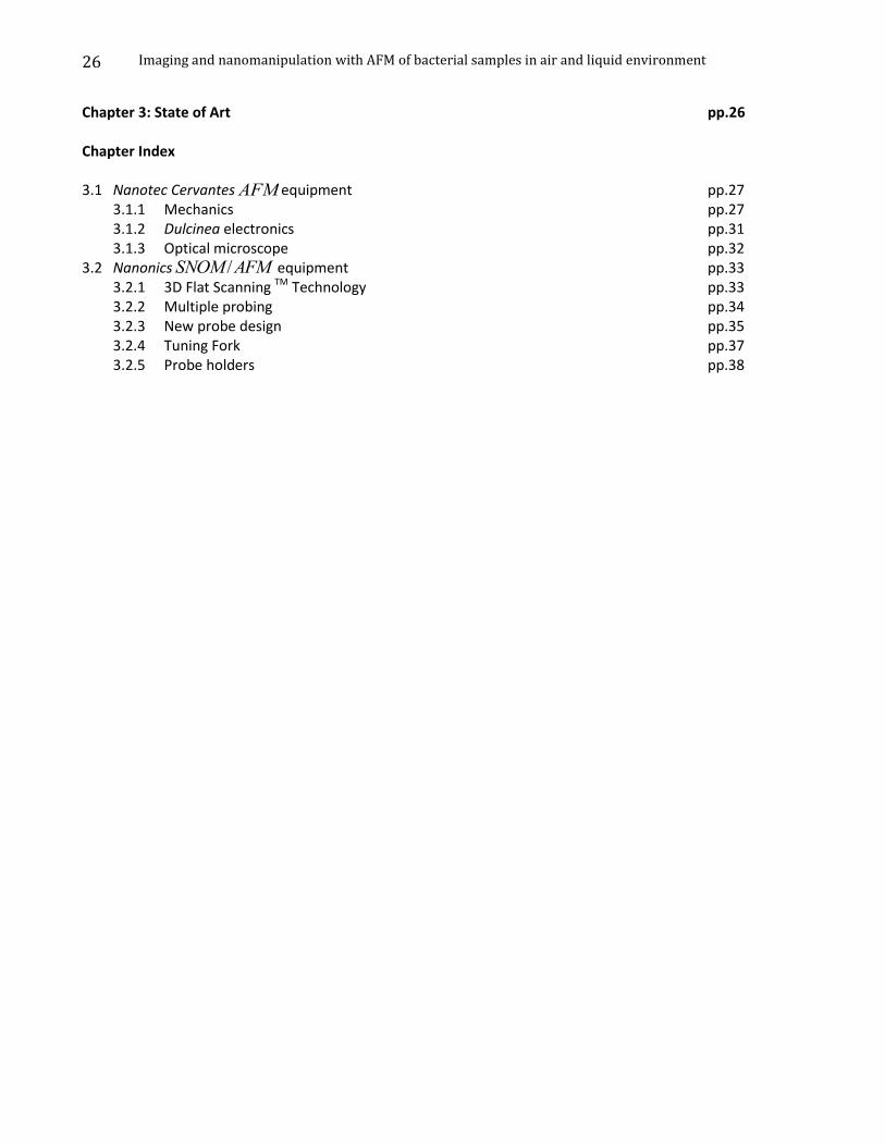
Thus it is possible to emphasize small-scale topography inequalities. Even more, WSxM (Software
controlling Cervantes Nanotec AFM), can create scaling and rotation of acquired AFM images. In
(2D) visualization (also named ″Top View″ image) to each point of the surface Z f (x,y) is
assigned a color (or a brightness) that corresponds to its z-value according to a given color-scale (or
gray-scale). As an example, the (2D)image of a surface area is presented on Image 2.13.
Image 2.13 2D brightness image of surface topography of image 2.12.

Imaging and nanomanipulation with AFM of bacterial samples in air and liquid environment
25
In general, the physical meaning of the SPM images depend on the parameter that is used in the
feedback loop. For example, the values stored in the Z f (x,y)matrix may depend on:
The electric current value flowing through the tip-surface contact with constant applied
voltage (STM) .
The main tip-surface interactive force in case is electric than is EFM, and in case is magnetic
is called MFM.
Besides these “maps” of the tip-sample interaction over the scanned area, a different type of
information may be retrieved using SPM. For example, on a single point of the sample surface we
may collect the dependence of the tunneling current on the applied voltage, the dependence of the
interactive force on the tip-sample distance, etc.
This information is stored as vector files or as matrixes of 2 N dimension, that may be displayed or
printed using a set of standard tools for graphic presentation provided by the generic AFM /SPM
software that we are using. SPM images, alongside with the helpful information, contain also a lot
of secondary information affecting the data and appearing as image distortions. Possible distortions
in SPM images caused by imperfection of the equipment and by external parasitic influences can be
eliminated by some general treatments like: subtraction of a constant component or constant
inclination, elimination of the distortions due to scanner imperfection, median filtering, line
averaging and Fourier filtration of the SPM images, surface restoration using a known tip shape, etc.
Imaging and nanomanipulation with AFM of bacterial samples in air and liquid environment
26
Chapter 3: State of Art pp.26 Chapter Index 3.1 Nanotec Cervantes AFM equipment pp.27
3.1.1 Mechanics pp.27 3.1.2 Dulcinea electronics pp.31 3.1.3 Optical microscope pp.32
3.2 Nanonics SNOM /AFM equipment pp.33 3.2.1 3D Flat Scanning TM Technology pp.33 3.2.2 Multiple probing pp.34 3.2.3 New probe design pp.35 3.2.4 Tuning Fork pp.37 3.2.5 Probe holders pp.38
Imaging and nanomanipulation with AFM of bacterial samples in air and liquid environment
27
Is normal that during your training period, there is need for participating in meetings, workshops,
congresses etc. Because in this ambient you find people working in the same field as you. People
with more o less the same interests as you but the most important thing is that there will be always
a researcher who has been in the same difficulties as you.
So, what a perfect moment for exchanging ideas and frustrations! But, despite jokes, these meetings
are really important and can give a solution or redirect your research line in the proper direction, as
happened to me.
The International SPMuser meeting organized by Scientec (Agilent Technologies) [16] gave me the
possibility to meet different firms producing near field microscopes like: Nanonics [17], Agilent
Technologies [18] and NanoSurf [19].Leaders in :optical, near field, and SPM.
3.1 Nanotec Cervantes AFM equipment
3.1.1 Mechanics
Nanotec AFM mechanical system can be divided into two main parts: chassis and head. Image 3.1
(gentle courtesy of Nanotec Electronica[20]) represents the AFM chassis, a general view of the
different elements that integrate the mechanics, pointing out their different components:
Image 3.1 Chassis
Imaging and nanomanipulation with AFM of bacterial samples in air and liquid environment
28
Let’s explain shortly each part’s function:
Beneath the motor base stands the micrometric motor, which rotates the micrometric
screws for approaching and withdrawing the AFM head from the sample. In this way the
cantilever holder, held in the AFM head, approaches the sample carried on the top of piezo
scanner.
Piezo scanner is the place where is situated the piezoresistive part of scanner. Is a cylindrical
space where is introduced the piezo as shown in Image 3.5.
The micrometric screws are used to move the whole chassis with micrometric precision
during the optical phase. Depending on the optical microscope sometimes isn’t possible to
move it laterally with micrometric precision. In this way the chassis design permits us to go
through optical microscope limitations for a better optical visualization of the tip/sample.
Image 3.2 is an upper vision of the chassis, and it’s interconnections with Dulcinea electronics.
Image 3.2 AFM Chassis.
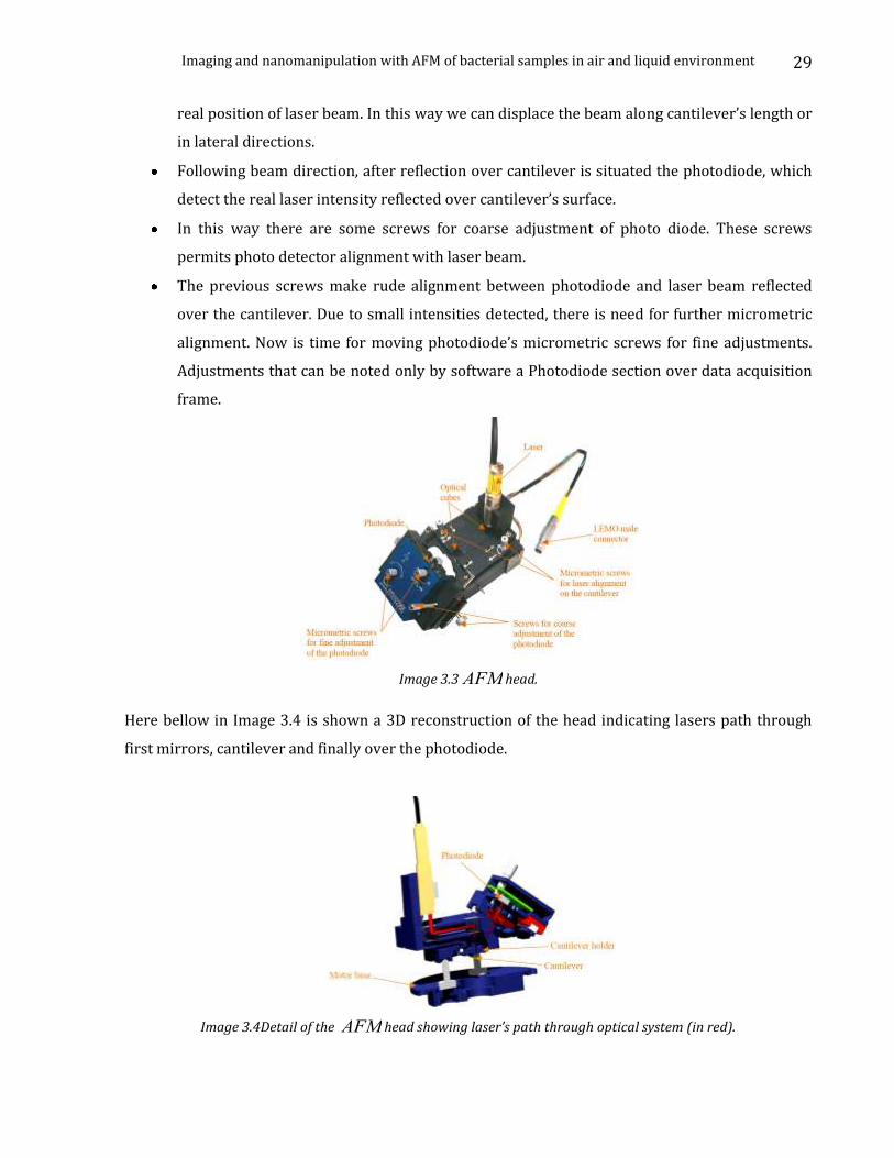
Meanwhile the other important part of AFM mechanics is illustrated in Image 3.3. AFM head hold
the cantilever and is situated over three micrometric screws. Two of them are in a frontal position
and ensures the planar holder collocation respect to the sample. The third one is controlled by
software and is moved from the motor.
With arrows are represented the main important parts of the head:
The laser is situated in vertical direction injecting its beam directly to a couple of mirrors
redirecting it over the cantilevers holder (See Image 3.4).
There are micrometric screws for laser alignment on the cantilever. Useful for detecting the
Imaging and nanomanipulation with AFM of bacterial samples in air and liquid environment
29
real position of laser beam. In this way we can displace the beam along cantilever’s length or
in lateral directions.
Following beam direction, after reflection over cantilever is situated the photodiode, which
detect the real laser intensity reflected over cantilever’s surface.
In this way there are some screws for coarse adjustment of photo diode. These screws
permits photo detector alignment with laser beam.
The previous screws make rude alignment between photodiode and laser beam reflected
over the cantilever. Due to small intensities detected, there is need for further micrometric
alignment. Now is time for moving photodiode’s micrometric screws for fine adjustments.
Adjustments that can be noted only by software a Photodiode section over data acquisition
frame.
Image 3.3 AFM head.
Here bellow in Image 3.4 is shown a 3D reconstruction of the head indicating lasers path through
first mirrors, cantilever and finally over the photodiode.
Image 3.4Detail of the AFM head showing laser’s path through optical system (in red).

Imaging and nanomanipulation with AFM of bacterial samples in air and liquid environment
30
The piezo scanners are responsible for movement of the sample in x, y and z directions.
Image 3.5 Piezo scanners (long and short).
Image 3.6 is a photo of a generic Cervantes Nanotecholder. In the central channel is situated
cantilevers deposit. In this demo is collocated a cantilever for demonstrating it’s correct placement
(Orange circle).
Image 3.6 Cantilever holder.
With the system is also provided a glass cover, which allows covering all the system to protect from
acoustic and environmental noises, as well as to perform atmosphere control as: humidity,
temperature, gas concentrations etc.
Image 3.7 AFM head glass cover and cantilever exchange bay.
In Image 3.8 is shown the metallic base and fork for an easy cantilever placing or removal when
using the elastic stripes to fix it to the cantilever holder.
Once correctly placed the microchip over the holder, it’s time to situate holder in the AFM head. In
Image 3.8 is a photo of the AFM head with holder correctly placed. Is easy to detect if is correctly
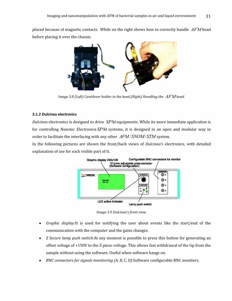
Imaging and nanomanipulation with AFM of bacterial samples in air and liquid environment
31
placed because of magnetic contacts. While on the right shows how to correctly handle AFM head
before placing it over the chassis.
Image 3.8 (Left) Cantilever holder in the head.(Right) Handling the AFM head.
3.1.2 Dulcinea electronics
Dulcinea electronics is designed to drive SPM equipments. While its more immediate application is
for controlling Nanotec Electronica SPM systems, it is designed in an open and modular way in
order to facilitate the interfacing with any other AFM /SNOM /STM system.
In the following pictures are shown the front/back views of Dulcinea’s electronics, with detailed
explanation of use for each visible part of it.
Image 3.9 Dulcinea’s front view.
Graphic display:It is used for notifying the user about events like the start/end of the
communication with the computer and the gains changes.
Z Secure lamp push switch:At any moment is possible to press this button for generating an
offset voltage of +150V to the Z piezo voltage. This allows fast withdrawal of the tip from the
sample without using the software. Useful when software hangs on.
BNC connectors for signals monitoring (A, B, C, D):Software configurable BNC monitors.
Imaging and nanomanipulation with AFM of bacterial samples in air and liquid environment
32
Image 3.10 Dulcinea’s back view.
BNC connectors:target specific BNC monitors and BNCs for external inputs:
VCO Out:Driving signal for cantilever oscillation (+/-10V).
I. Out:Driving signal for magnetic cantilever oscillation. It is an AC current source with the
same frequency as the VCO Out (selected in the WSxM tapping menu).
Ext. In: [Input signal].Allows introducing an external signal as the dynamic mode reference
signal (+/- 10V).
3.1.3 Optical microscope
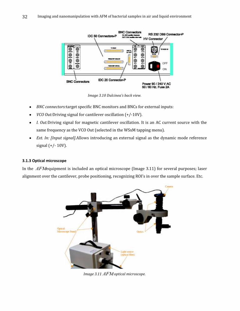
In the AFMequipment is included an optical microscope (Image 3.11) for several purposes; laser
alignment over the cantilever, probe positioning, recognizing ROI’s in over the sample surface. Etc.
Image 3.11 AFM optical microscope.
Imaging and nanomanipulation with AFM of bacterial samples in air and liquid environment
33
3.2 Nanonics NSOM /AFM equipment
Nanonics equipment integrates AFM /SNOM microscopes. There is the intent to include more
than one microscopy technologies in one compound microscope, the so-called Multiple Probe
SNOM/SPM systems. They have achieved several good results and we are going to list some of
them:
No need for a laser beam monitoring cantilevers deflection (tuning fork principle).
3D Flat Scanning TM Technology.
Ability to integrate up to four probes in one microscope.
Their huge flexibility in different types of probes.
Complete integration of SEM /SPM .
Simultaneous On-Line AFM and Confocal microscopy.
The first to integrate AFM /Raman microscopy (patented).
Possibility to follow optically above and bellow the sample.
In the following paragraphs we will illustrate the solutions adopted from Nanonics (All the images of
MultiVew4000 are a gentle courtesy of Dr. David Lewis, Nanonics vice-president).
3.2.1 3D Flat Scanning TM Technology
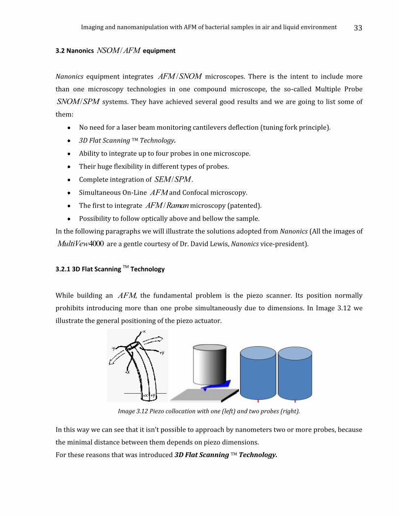
While building an AFM, the fundamental problem is the piezo scanner. Its position normally
prohibits introducing more than one probe simultaneously due to dimensions. In Image 3.12 we
illustrate the general positioning of the piezo actuator.
Image 3.12 Piezo collocation with one (left) and two probes (right).
In this way we can see that it isn’t possible to approach by nanometers two or more probes, because
the minimal distance between them depends on piezo dimensions.
For these reasons that was introduced 3D Flat Scanning TM Technology.

Imaging and nanomanipulation with AFM of bacterial samples in air and liquid environment
34
Nanonicssolution was, developing a scanner with a geometry that allow great flexibility in multi-
probe design, while providing optically and electron/ion optically friendly systems that can fit any
optically based technique such as Raman [21] or electron optically based techniques such as a SEM
[22] or ion optical technique such as an FIB [23] or for that matter even in SEM /FIB systems.
This technology provides:
A novel planar, folded-piezo, flexible scan design with their advantages.
Allows large simultaneous lateral and axial sample scanning.
Ultrathin scanner can be incorporated into systems where conventional scan stages are too
bulky and geometrically limiting
The minimal stage height of 7 mm allows for easy access with high-powered microscope
objectives from either above or below the scanning stages.
The large vertical (axial) displacement of up to 100 microns allows for multiple probes and
allows for tracking of structures with very large topographical features.
Image 3.13 3D FlatScan™ technology.
Its main features are:
>20 mm clear axis.
7 mm thin scanners.
100 micron 3D fine scanning in X, Y and Z directions.
3.2.2 Multiple probing
In Image 3.14 is shown MultiVew4000 with one, two and four probes installed. It has a geometry
directed toward an open architecture, and for scattering NSOMexperiments with piezo control of
the tip while the tip is scanning for ultra-accurate positioning of the tip in a laser beam and in
addition sample scanning.
As we mentioned above, it has a completely free optical axis from above and below and with open
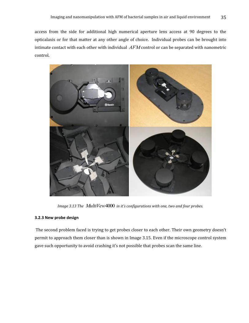
Imaging and nanomanipulation with AFM of bacterial samples in air and liquid environment
35
access from the side for additional high numerical aperture lens access at 90 degrees to the
opticalaxis or for that matter at any other angle of choice. Individual probes can be brought into
intimate contact with each other with individual AFM control or can be separated with nanometric
control.
Image 3.13 The MultiVew4000 in it’s configurations with one, two and four probes.
3.2.3 New probe design
The second problem faced is trying to get probes closer to each other. Their own geometry doesn’t
permit to approach them closer than is shown in Image 3.15. Even if the microscope control system
gave such opportunity to avoid crashing it’s not possible that probes scan the same line.

Imaging and nanomanipulation with AFM of bacterial samples in air and liquid environment
36
Image 3.14 Distance between tips approaching each other.
Nanonics has developed spatially and optically friendly glass based probes that allow a close
approach of the probe tips, crucial for multi-probe imaging systems. Also these probes offer good
imaging not only in AFM modes but as will be indicated further, specialized glass probes also
allow; singular electrical imaging, thermal imaging and chemical writing. The probes have
unparalleled aspect ratios and allow for deep trench imaging and even sidewall imaging. Tip
geometry and parameters are illustrated in Image 3.16.
Image 3.15 Glass tip dimensions.
But this firm has been producing too, other types of probes like: thermal conductivity probes; wired
electrical probes, glass probes, tuning fork probes etc.
Image 3.16 NSOM, wired, glass and thermal conductivity probes.
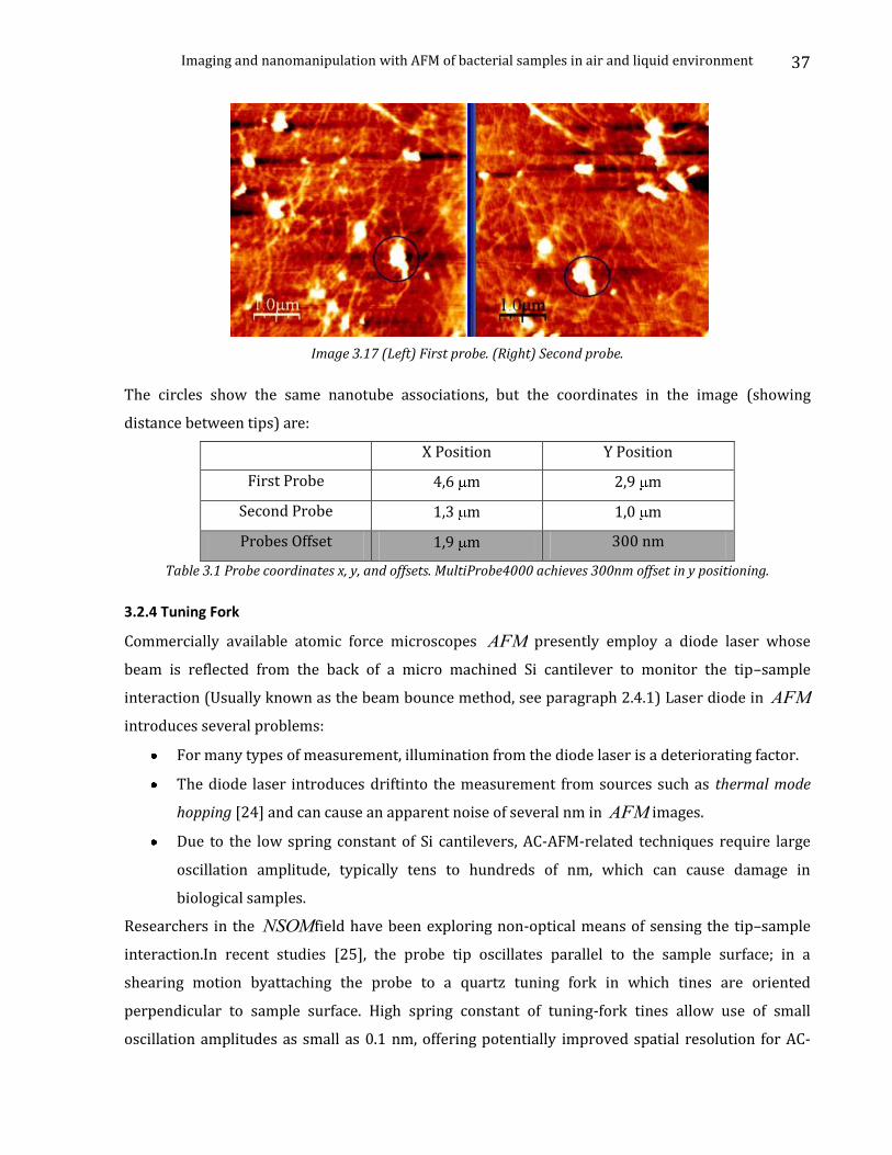
In the following, (Image 3.18) are two images presenting simultaneous imaging of carbon nanotubes
with two probes. On the left there is an image taken from the first probe and on the right the image
taken from the second probe.
Imaging and nanomanipulation with AFM of bacterial samples in air and liquid environment
37
Image 3.17 (Left) First probe. (Right) Second probe.
The circles show the same nanotube associations, but the coordinates in the image (showing
distance between tips) are:
X Position Y Position
First Probe 4,6 m 2,9 m
Second Probe 1,3 m 1,0 m
Probes Offset 1,9 m 300 nm
Table 3.1 Probe coordinates x, y, and offsets. MultiProbe4000 achieves 300nm offset in y positioning.
3.2.4 Tuning Fork
Commercially available atomic force microscopes AFM presently employ a diode laser whose
beam is reflected from the back of a micro machined Si cantilever to monitor the tip–sample
interaction (Usually known as the beam bounce method, see paragraph 2.4.1) Laser diode in AFM
introduces several problems:
For many types of measurement, illumination from the diode laser is a deteriorating factor.
The diode laser introduces driftinto the measurement from sources such as thermal mode
hopping [24] and can cause an apparent noise of several nm in AFM images.
Due to the low spring constant of Si cantilevers, AC-AFM-related techniques require large
oscillation amplitude, typically tens to hundreds of nm, which can cause damage in
biological samples.
Researchers in the NSOMfield have been exploring non-optical means of sensing the tip–sample
interaction.In recent studies [25], the probe tip oscillates parallel to the sample surface; in a
shearing motion byattaching the probe to a quartz tuning fork in which tines are oriented
perpendicular to sample surface. High spring constant of tuning-fork tines allow use of small
oscillation amplitudes as small as 0.1 nm, offering potentially improved spatial resolution for AC-
Imaging and nanomanipulation with AFM of bacterial samples in air and liquid environment
38
AFM-related techniques.In AFM, the great advantage of using such smaller oscillating amplitudes
is when imaging biological samples. Small excitation amplitudes imply less force applied to the
sample. In this way is possible to measure the real dimensions or at the worst case to avoid
destroying soft samples as: proteins, DNA etc.
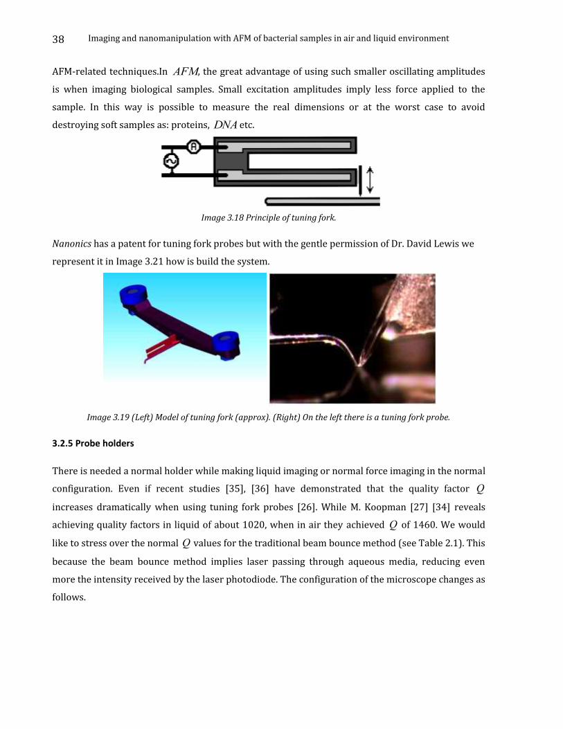
Image 3.18 Principle of tuning fork.
Nanonics has a patent for tuning fork probes but with the gentle permission of Dr. David Lewis we
represent it in Image 3.21 how is build the system.
Image 3.19 (Left) Model of tuning fork (approx). (Right) On the left there is a tuning fork probe.
3.2.5 Probe holders
There is needed a normal holder while making liquid imaging or normal force imaging in the normal
configuration. Even if recent studies [35], [36] have demonstrated that the quality factor Q
increases dramatically when using tuning fork probes [26]. While M. Koopman [27] [34] reveals
achieving quality factors in liquid of about 1020, when in air they achieved Q of 1460. We would
like to stress over the normal Q values for the traditional beam bounce method (see Table 2.1). This
because the beam bounce method implies laser passing through aqueous media, reducing even
more the intensity received by the laser photodiode. The configuration of the microscope changes as
follows.
Imaging and nanomanipulation with AFM of bacterial samples in air and liquid environment
39
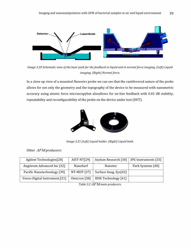
Image 3.20 Schematic view of the laser path for the feedback in liquid and in normal force imaging. (Left) Liquid
imaging. (Right) Normal force.
In a close up view of a mounted Nanonics probe we can see that the cantilevered nature of the probe
allows for not only the geometry and the topography of the device to be measured with nanometric
accuracy using atomic force microscopybut alsoallows for on-line feedback with 0.02 dB stability,
repeatability and reconfigurability of the probe on the device under test (DUT).
Image 3.21 (Left) Liquid holder. (Right) Liquid bath.
Other AFM producers:
Agilent Technologies[28] AIST-NT[29] Asylum Research [30] JPK Instruments [33]
Angstrom Advanced Inc [32] NanoSurf Nanotec Park Systems [40]
Pacific Nanotechnology [39] NT-MDT [37] Surface Imag. Sys[42]
Veeco-Digital Instrument.[31] Omicron [38] RHK Technology [41]
Table 3.2 AFM main producers.
Imaging and nanomanipulation with AFM of bacterial samples in air and liquid environment
40
Chapter 4: Imaging techniques pp.40 Chapter Index 4.1 Brief tutorial over WSxM pp.41
4.1.1 Getting started pp.41 4.1.2 Laser and photodiode calibration pp.42 4.1.3 Contact Mode pp.45 4.1.4 Dynamic Mode AC pp.48 4.1.5 Jumping Mode pp.52 4.1.6 Artifacts pp.54
4.2 Gnome for Scanning Microscopy (GxSM) pp.57 4.2.1 DSP controller pp.57 4.2.2 Instalation of Signal Ranger Board & Gxsm (ver 1.9) pp.57 4.2.3 Brief tutorial of GxSM pp.60
Imaging and nanomanipulation with AFM of bacterial samples in air and liquid environment
41
4.1 Brief tutorial over WSxM
In the following paragraphs it will be described, as a compound number of steps, how to start an
imaging section. We refer to WSxM ver.12.1 (September 2008).
4.1.1 Getting started
The following steps illustrate how to get started using the WSxM software.
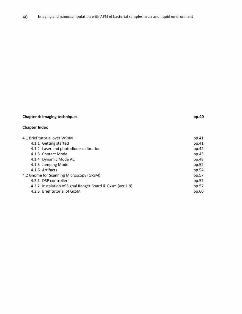
Turn on the Computer for data acquisition.
Turn on the Dulcinea Control unit. (Turn on the red switch at rear part)
Start control-program WSxM.
The first screen shows whether all parts of the system are properly connected and ready to work.
The program can also be started in simulation mode without AFM and control unit.
Image 4.1 First frame of WSxM.
Imaging and nanomanipulation with AFM of bacterial samples in air and liquid environment
42
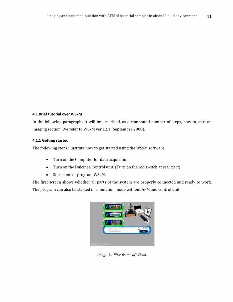
Click onto the symbol “DA” – Data acquisition and afterwards the button “Go” in the upper control
bar. The acquisition process is started now. The following window (or similar) should be displayed:
Image 4.2 Screening of the Acquisition mode of WSxM.
On the left side we see a control panel that shows the parameters of the scanning process. Let’s have
a closer look onto this panel and see what the meaning of these parameters is.
Image 4.3 Main Control Panel.
4.1.2 Laser and photodiode calibration
Size: in nm of the squared zone that is scanned.
Freq: number of lines that is scanned per second in x direction.
Points: number of lines that contain the square
X/Y/Z off: offset
Angle: in x-y plane the scan is performed, in order to get a good
scan, angle should be modified so that each scan line is in a
plane.
Bias: Voltage applied between tip an sample.
Set Point: feedback is performed to adjust the feedback
parameter to this value.
Z Gain: defines the margin in which the z-piezo can extend.
Imaging and nanomanipulation with AFM of bacterial samples in air and liquid environment
43
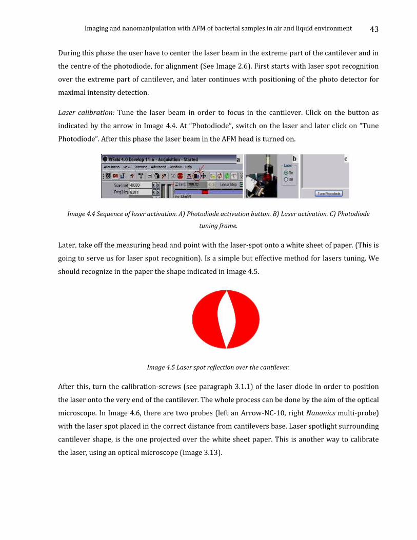
During this phase the user have to center the laser beam in the extreme part of the cantilever and in
the centre of the photodiode, for alignment (See Image 2.6). First starts with laser spot recognition
over the extreme part of cantilever, and later continues with positioning of the photo detector for
maximal intensity detection.
Laser calibration: Tune the laser beam in order to focus in the cantilever. Click on the button as
indicated by the arrow in Image 4.4. At “Photodiode”, switch on the laser and later click on “Tune
Photodiode”. After this phase the laser beam in the AFM head is turned on.
Image 4.4 Sequence of laser activation. A) Photodiode activation button. B) Laser activation. C) Photodiode
tuning frame.
Later, take off the measuring head and point with the laser-spot onto a white sheet of paper. (This is
going to serve us for laser spot recognition). Is a simple but effective method for lasers tuning. We
should recognize in the paper the shape indicated in Image 4.5.
Image 4.5 Laser spot reflection over the cantilever.
After this, turn the calibration-screws (see paragraph 3.1.1) of the laser diode in order to position
the laser onto the very end of the cantilever. The whole process can be done by the aim of the optical
microscope. In Image 4.6, there are two probes (left an Arrow-NC-10, right Nanonics multi-probe)
with the laser spot placed in the correct distance from cantilevers base. Laser spotlight surrounding
cantilever shape, is the one projected over the white sheet paper. This is another way to calibrate
the laser, using an optical microscope (Image 3.13).
Imaging and nanomanipulation with AFM of bacterial samples in air and liquid environment
44
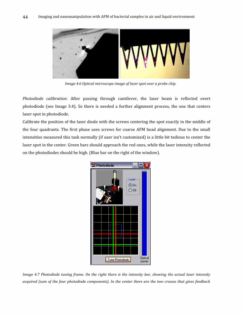
Image 4.6 Optical microscope image of laser spot over a probe chip.
Photodiode calibration: After passing through cantilever, the laser beam is reflected overt
photodiode (see Image 3.4). So there is needed a further alignment process, the one that centers
laser spot in photodiode.
Calibrate the position of the laser diode with the screws centering the spot exactly in the middle of
the four quadrants. The first phase uses screws for coarse AFM head alignment. Due to the small
intensities measured this task normally (if user isn’t customized) is a little bit tedious to center the
laser spot in the center. Green bars should approach the red ones, while the laser intensity reflected
on the photodiodes should be high. (Blue bar on the right of the window).
Image 4.7 Photodiode tuning frame. On the right there is the intensity bar, showing the actual laser intensity
acquired (sum of the four photodiode components). In the center there are the two crosses that gives feedback

Imaging and nanomanipulation with AFM of bacterial samples in air and liquid environment
45
over the coarse movements induced to photodiode. In this way, when both red crosses are inside square, appear
green crosses. They help for fine adjustments and should overlap the red ones.
This is as a result of the following configuration a disposition of the photodiode.
As the photodiode is compound of four pieces (lets call them 1,2,3 and 4), the resulting intensity of
the laser beam is a composition of the four intensities of each piece. In Image 4.8, is shown how is
calculated the resulting intensity. While linear combinations of them gives more information
regarding Normal and Lateral forces.
Hint: The total intensity received at the photodiode (blue bar), depends on different factors such as
geography of cantilever, dimensions of cantilever etc… As a consequence, not always will be
possible to have maximum height of the bar. Is considered god one, which is higher than 2/3 of
maximum height.
Image 4.8 Calculation of Normal and lateral force from laser photodiode sections.
4.1.3 Contact Mode
In contact mode the feedback is performed on the normal force that is the vertical deflection of the
laser spot in the photodiode. When the tip gets into contact with the surface, the cantilever will bend
and deflect the laser beam into this direction.
Approach: Click onto the button “Approach” and open the approach-menu. Choose a Set Point
slightly higher (10-20 %) than the actual normal-force value.
Imaging and nanomanipulation with AFM of bacterial samples in air and liquid environment
46
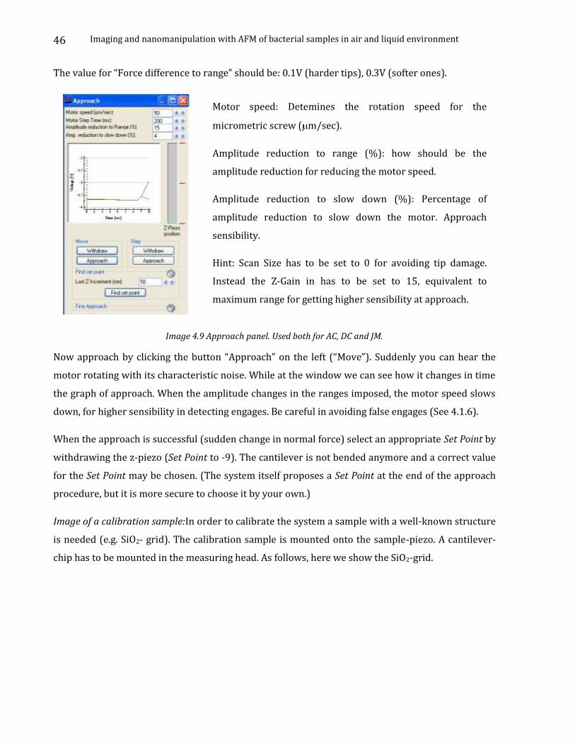
The value for “Force difference to range” should be: 0.1V (harder tips), 0.3V (softer ones).
Image 4.9 Approach panel. Used both for AC, DC and JM.
Now approach by clicking the button “Approach” on the left (“Move”). Suddenly you can hear the
motor rotating with its characteristic noise. While at the window we can see how it changes in time
the graph of approach. When the amplitude changes in the ranges imposed, the motor speed slows
down, for higher sensibility in detecting engages. Be careful in avoiding false engages (See 4.1.6).
When the approach is successful (sudden change in normal force) select an appropriate Set Point by
withdrawing the z-piezo (Set Point to -9). The cantilever is not bended anymore and a correct value
for the Set Point may be chosen. (The system itself proposes a Set Point at the end of the approach
procedure, but it is more secure to choose it by your own.)
Image of a calibration sample:In order to calibrate the system a sample with a well-known structure
is needed (e.g. SiO2- grid). The calibration sample is mounted onto the sample-piezo. A cantilever-
chip has to be mounted in the measuring head. As follows, here we show the SiO2-grid.
Motor speed: Detemines the rotation speed for the
micrometric screw ( m/sec).
Amplitude reduction to range (%): how should be the
amplitude reduction for reducing the motor speed.
Amplitude reduction to slow down (%): Percentage of
amplitude reduction to slow down the motor. Approach
sensibility.
Hint: Scan Size has to be set to 0 for avoiding tip damage.
Instead the Z-Gain in has to be set to 15, equivalent to
maximum range for getting higher sensibility at approach.
Imaging and nanomanipulation with AFM of bacterial samples in air and liquid environment
47
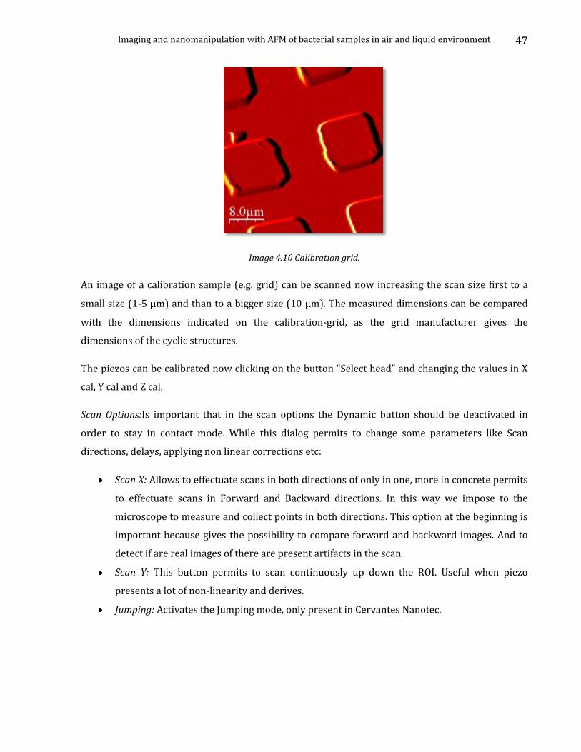
Image 4.10 Calibration grid.
An image of a calibration sample (e.g. grid) can be scanned now increasing the scan size first to a
small size (1-5 m) and than to a bigger size (10 m). The measured dimensions can be compared
with the dimensions indicated on the calibration-grid, as the grid manufacturer gives the
dimensions of the cyclic structures.
The piezos can be calibrated now clicking on the button “Select head” and changing the values in X
cal, Y cal and Z cal.
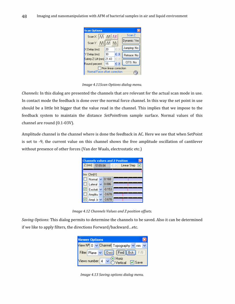
Scan Options:Is important that in the scan options the Dynamic button should be deactivated in
order to stay in contact mode. While this dialog permits to change some parameters like Scan
directions, delays, applying non linear corrections etc:
Scan X: Allows to effectuate scans in both directions of only in one, more in concrete permits
to effectuate scans in Forward and Backward directions. In this way we impose to the
microscope to measure and collect points in both directions. This option at the beginning is
important because gives the possibility to compare forward and backward images. And to
detect if are real images of there are present artifacts in the scan.
Scan Y: This button permits to scan continuously up down the ROI. Useful when piezo
presents a lot of non-linearity and derives.
Jumping: Activates the Jumping mode, only present in Cervantes Nanotec.
Imaging and nanomanipulation with AFM of bacterial samples in air and liquid environment
48
Image 4.11Scan Options dialog menu.
Channels: In this dialog are presented the channels that are relevant for the actual scan mode in use.
In contact mode the feedback is done over the normal force channel. In this way the set point in use
should be a little bit bigger that the value read in the channel. This implies that we impose to the
feedback system to maintain the distance SetPointfrom sample surface. Normal values of this
channel are round (0.1-03V).
Amplitude channel is the channel where is done the feedback in AC. Here we see that when SetPoint
is set to -9, the current value on this channel shows the free amplitude oscillation of cantilever
without presence of other forces (Van der Waals, electrostatic etc.)
Image 4.12 Channels Values and Z position offsets.
Saving Options: This dialog permits to determine the channels to be saved. Also it can be determined
if we like to apply filters, the directions Forward/backward…etc.
Image 4.13 Saving options dialog menu.
Imaging and nanomanipulation with AFM of bacterial samples in air and liquid environment
49
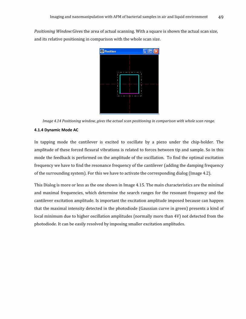
Positioning Window:Gives the area of actual scanning. With a square is shown the actual scan size,
and its relative positioning in comparison with the whole scan size.
Image 4.14 Positioning window, gives the actual scan positioning in comparison with whole scan range.
4.1.4 Dynamic Mode AC
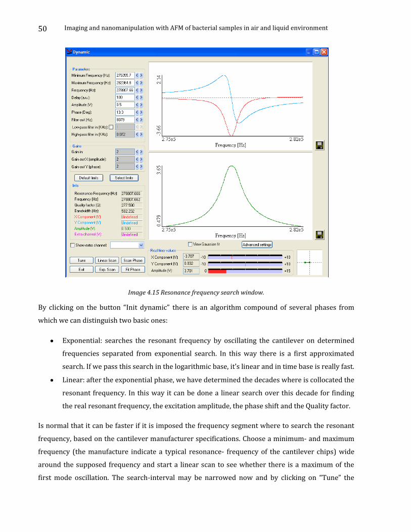
In tapping mode the cantilever is excited to oscillate by a piezo under the chip-holder. The
amplitude of these forced flexural vibrations is related to forces between tip and sample. So in this
mode the feedback is performed on the amplitude of the oscillation. To find the optimal excitation
frequency we have to find the resonance frequency of the cantilever (adding the damping frequency
of the surrounding system). For this we have to activate the corresponding dialog (Image 4.2).
This Dialog is more or less as the one shown in Image 4.15. The main characteristics are the minimal
and maximal frequencies, which determine the search ranges for the resonant frequency and the
cantilever excitation amplitude. Is important the excitation amplitude imposed because can happen
that the maximal intensity detected in the photodiode (Gaussian curve in green) presents a kind of
local minimum due to higher oscillation amplitudes (normally more than 4V) not detected from the
photodiode. It can be easily resolved by imposing smaller excitation amplitudes.
Imaging and nanomanipulation with AFM of bacterial samples in air and liquid environment
50
Image 4.15 Resonance frequency search window.
By clicking on the button “Init dynamic” there is an algorithm compound of several phases from
which we can distinguish two basic ones:
Exponential: searches the resonant frequency by oscillating the cantilever on determined
frequencies separated from exponential search. In this way there is a first approximated
search. If we pass this search in the logarithmic base, it’s linear and in time base is really fast.
Linear: after the exponential phase, we have determined the decades where is collocated the
resonant frequency. In this way it can be done a linear search over this decade for finding
the real resonant frequency, the excitation amplitude, the phase shift and the Quality factor.
Is normal that it can be faster if it is imposed the frequency segment where to search the resonant
frequency, based on the cantilever manufacturer specifications. Choose a minimum- and maximum
frequency (the manufacture indicate a typical resonance- frequency of the cantilever chips) wide
around the supposed frequency and start a linear scan to see whether there is a maximum of the
first mode oscillation. The search-interval may be narrowed now and by clicking on “Tune” the

Imaging and nanomanipulation with AFM of bacterial samples in air and liquid environment
51
resonance-frequency will be determined automatically and applied on the system for
measurements. Close the window by pressing “Exit”.
Hint: Is good practice to control the phase shifts; if too big, press “Fit phase” for getting round zero
the phase shift.
Add the panel “Dynamic Settings” to the control panel. The excitation amplitude (V) has to be
chosen in a way that the cantilever swing just with an amplitude of some nanometers (5-10nm). The
system gets more sensitive the lower the amplitude of the oscillation is. When approaching the
sample surface the interactions between tip and sample lead to decreasing amplitude. So when
there is already small amplitude the detection of small force changes is easier. (To find out about the
oscillation amplitude see “force curves”.)
Since the amplitude is always displayed as a negative value the SetPoint in this mode has to be set
always to a negative value. High values (close to zero) mean a lot of applied force on the sample; low
values (e.g. -9) make the piezo to withdraw. It is dangerous to set a positive setpoint as the system
will probably damage the cantilever trying to get to this setpoint.
The feedback: - values in this mode are usually higher than in contact mode. The P.I corrections are
linear corrections and are implemented by the Lock-In amplifier present in the Dulcinea Electronics.
The correct values are relative depending on a lot of factors like: higher scan sizes (decreases P.I),
number of points per line (decreases P.I), Sample surface (the more rougher is the sample the less
adaptable to the changes is the system). It can bee changed the channel where is done the feedback
for different types of AFM (Contact, non contact, lateral force).
Image 4.16 Feedback control wondow.
Dynamic settings:In this dialog is possible to change the dynamic values like: Ampliude of oscillation,
frequency of oscillation activating PLL…etc.

Imaging and nanomanipulation with AFM of bacterial samples in air and liquid environment
52
Image 4.17 Dynamic settings dialog.
Force curves
Force curves may deliver some important information about the sample, the current operation
mode and the chosen parameters. In order to find the best operating parameters the different
scanning modes it may be suggestive to do a force curve on a sample point.
In our equipment it was possible to make Force Vs. Displacement curves only in the middle of the
actual scan line. This means that it’s not possible to determine the exact point where to make FZ.
This is one of the topics studied in chapter 6 where we, by means of Lithography section scripting,
determine the exact point where to make FZ curves.
First should be activated the “FZ”- dialog. In the force curve the deflection of the cantilever is
recorded in function of distance between sample and tip (z-position). In the picture such a force
curve for an approach and withdraw of the tip of 200nm is shown.
The FZ dialog has a lot of menus for higher performances, but we would like to emphasis over the
most used like: First Forward/Backward selection (Selects the direction of the FZ curve, if it
withdraws first the tip of approaches), Initial Z; explains the distance in nanometers of the first step,
and Oscillation Off; quits oscillation during FZ curves (results in the curves may vary the slope in the
linear stage).
While it can be modified the quantity of FZ curves done at once, and at the final result can be an
averaging of the N FZ curves done.
After “Do FZ”, in the Viewer, is shown the channels selected like; normal Vs. displacement, lateral Vs.
displacement, … etc. The channels can be selected from a pop up menu.
Imaging and nanomanipulation with AFM of bacterial samples in air and liquid environment
53
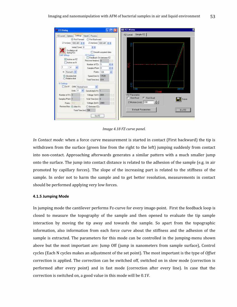
Image 4.18 FZ curve panel.
In Contact mode: when a force curve measurement is started in contact (First backward) the tip is
withdrawn from the surface (green line from the right to the left) jumping suddenly from contact
into non-contact. Approaching afterwards generates a similar pattern with a much smaller jump
onto the surface. The jump into contact distance is related to the adhesion of the sample (e.g. in air
promoted by capillary forces). The slope of the increasing part is related to the stiffness of the
sample. In order not to harm the sample and to get better resolution, measurements in contact
should be performed applying very low forces.
4.1.5 Jumping Mode
In jumping mode the cantilever performs Fz-curve for every image-point. First the feedback loop is
closed to measure the topography of the sample and then opened to evaluate the tip sample
interaction by moving the tip away and towards the sample. So apart from the topographic
information, also information from each force curve about the stiffness and the adhesion of the
sample is extracted. The parameters for this mode can be controlled in the jumping-menu shown
above but the most important are: Jump Off (jump in nanometers from sample surface), Control
cycles (Each N cycles makes an adjustment of the set point). The most important is the type of Offset
correction is applied. The correction can be switched off, switched on in slow mode (correction is
performed after every point) and in fast mode (correction after every line). In case that the
correction is switched on, a good value in this mode will be 0.1V.
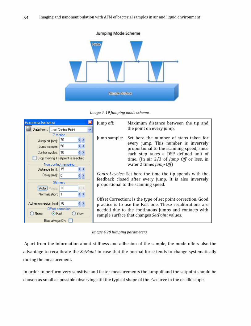
Imaging and nanomanipulation with AFM of bacterial samples in air and liquid environment
54
Image 4. 19 Jumping mode scheme.
Image 4.20 Jumping parameters.
Apart from the information about stiffness and adhesion of the sample, the mode offers also the
advantage to recalibrate the SetPoint in case that the normal force tends to change systematically
during the measurement.
In order to perform very sensitive and faster measurements the jumpoff and the setpoint should be
chosen as small as possible observing still the typical shape of the Fz-curve in the oscilloscope.
Jump off: Maximum distance between the tip and the point on every jump.
Jump sample: Set here the number of steps taken for every jump. This number is inversely proportional to the scanning speed, since each step takes a DSP defined unit of time. (In air 2/3 of Jump Off or less, in water 2 times Jump Off)
Control cycles: Set here the time the tip spends with the feedback closed after every jump. It is also inversely proportional to the scanning speed.
Offset Correction: Is the type of set point correction. Good practice is to use the Fast one. These recalibrations are needed due to the continuous jumps and contacts with sample surface that changes SetPoint values.
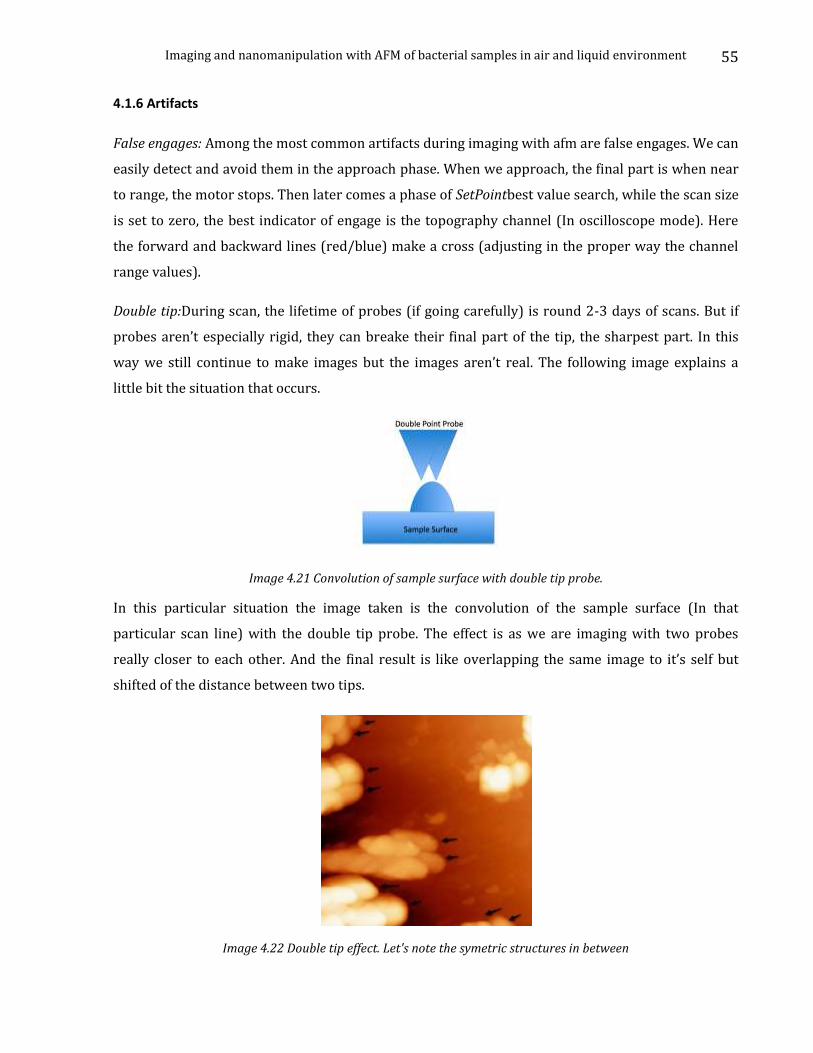
Imaging and nanomanipulation with AFM of bacterial samples in air and liquid environment
55
4.1.6 Artifacts
False engages: Among the most common artifacts during imaging with afm are false engages. We can
easily detect and avoid them in the approach phase. When we approach, the final part is when near
to range, the motor stops. Then later comes a phase of SetPointbest value search, while the scan size
is set to zero, the best indicator of engage is the topography channel (In oscilloscope mode). Here
the forward and backward lines (red/blue) make a cross (adjusting in the proper way the channel
range values).
Double tip:During scan, the lifetime of probes (if going carefully) is round 2-3 days of scans. But if
probes aren’t especially rigid, they can breake their final part of the tip, the sharpest part. In this
way we still continue to make images but the images aren’t real. The following image explains a
little bit the situation that occurs.
Image 4.21 Convolution of sample surface with double tip probe.
In this particular situation the image taken is the convolution of the sample surface (In that
particular scan line) with the double tip probe. The effect is as we are imaging with two probes
really closer to each other. And the final result is like overlapping the same image to it’s self but
shifted of the distance between two tips.
Image 4.22 Double tip effect. Let's note the symetric structures in between
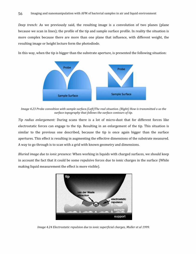
Imaging and nanomanipulation with AFM of bacterial samples in air and liquid environment
56
Deep trench: As we previously said, the resulting image is a convolution of two planes (plane
because we scan in lines); the profile of the tip and sample surface profile. In reality the situation is
more complex because there are more than one plane that influence, with different weight, the
resulting image or height lecture form the photodiode.
In this way, when the tip is bigger than the substrate aperture, is presented the following situation:
Image 4.23 Probe convoltion with sample surface.(Left)The real situation. (Right) How is transmitted o us the surface topography that follows the surface contours of tip.
Tip radius enlargement: During scans there is a lot of micro-dust that for different forces like
electrostatic forces can engage to the tip. Resulting in an enlargement of the tip. This situation is
similar to the previous one described, because the tip is once again bigger than the surface
apertures. This effect is resulting in augmenting the effective dimensions of the substrate measured.
A way to go through is to scan with a grid with known geometry and dimensions.
Bluried image due to ionic presence: When working in liquids with charged surfaces, we should keep
in account the fact that it could be some repulsive forces due to ionic charges in the surface (While
making liquid measurement the effect is more visible).
Image 4.24 Electrostatic repulsion due to ionic superficial charges, Muller et al 1999.
Imaging and nanomanipulation with AFM of bacterial samples in air and liquid environment
57
Trouble Shooting:
Low resolution. Everything seems to be quite blurred.
In this case, both in contact DC and jumping JM is better to increase the SetPoint in order to apply
more force between tip and sample, for gaining the repulsive forces. Be careful whether piezo is still
moving when varying the SetPoint.And as usual is good to make an Fz-curve. In tapping mode
increasing the excitation amplitude might help to get into contact with the sample. Once a stable
image is achieved the amplitude may be reduced again.
Water measurements: Apart from the advantage to do an image in a biological friendly
environment doing AFM-measurements in water (buffers) may also increase the resolution of the
images, as the influence of surface charges is reduced.
Mounting the tip holder for liquid measurements
A different tip holder has to be used for measurements in water. The disadvantages of this holder
are that vibrations performed by the small piezo in the holder for tapping-mode are noisier and in
general alignment of the laser-spot onto the tip is more complicated.
1. First, the tip should be cleaned the holder and putting a drop of vacuum fat onto the holder.
2. Take a new cantilever chip and “glue” it now onto the sample holder. The adhesion will be
strong enough to perform measurements.
The tip holder may be mounted onto the measuring-head and a rough alignment of the laser can be
done. The readily prepared sample has to be put onto the sample-holder. Wet the sample with a
(big) drop of buffer. Wet the tip-holder carefully from above to get a drop of buffer surrounding the
cantilever and protecting when approaching later to the sample. Mount the tip holder.
Approach the sample and tip manually (micrometer screws) until both drops (from tip and sample)
band together. The vertical alignment of the laser has changed now. So the laser has to be
recalibrated looking at the tip itself (throw the crystal-window in the tipholder) and the reflection
from the tip (typical refraction pattern when calibrated). Fine adjustment is done as usual with
intensity-meter of the photodiode in the software.
In general in water the whole measuring-setup has to equilibrate much more time than in
air. But with increasing time the risk of “tip-contamination” is also increasing, what will lead
to lower resolution. So in contrast to measurements in air there is a smaller time frame to
perform qualitatively high measurements.
Imaging and nanomanipulation with AFM of bacterial samples in air and liquid environment
58
Beginning measurements with a freshly mounted sample it maybe favorable to start in
jumping mode, as the automatic recalibration (SetPoint-correction) tends to be less harmless
for the sample.
For measurements in water the jump off may get as low as 20 nm. The value for the sample
rate should be twice the one of the jump off to stabilize the system.
In stable conditions measurements in contact mode may deliver the highest resolutions. It is
important to apply the lowest amount of force possible (also choosing the right tip).
4.2 GxSM
The GXSM is the Gnome X Scanning Microscopy project [43], [44] is SPM control and data analysis
software. It provides a solution for all homemade SPM; especially new prototypes intended to
invent new modes of operation, where the development of a complete new software system from
scratch would be too expensive and time consuming. Since GXSM is licensed under the GNU general
public license the full source code is published and everyone is allowed to use and modify the
software package for his own needs. The GXSM project has been developed under the GNU/Linux
operating system to a full-featured SPM software. The user interface is based on the modern
Gnome/Gtk1 library
4.2.1 DSP Controller
Using the PCI32 data acquisition board with the TMS320C32 [45] floating point DSP running at 60
MHz specialized DSP software is used to operate STM, AFM, and similar instruments. The design of
the DSP program is similar to a state machine and able to do quasimultitasking. All time dependent
tasks such as the feedback loop and certain signal generations are performed via hardware timer
driven interrupt subroutines to ensure proper timings.
Due to slightly different needs (e.g., logarithmic or linear feedback signals for STM or AFM,
respectively) optimized DSP codes are available for each supported instrument type. The DSP
source code (written almost completely in the ANSI C programming language) and precompiled DSP
binaries for several hardware configurations (ready to launch) are freely available.
4.2.2 Installation of Signal Ranger Board & GxSM (ver. 1.9)
Is important to have an updated linux kernel.
At the moment is used version (2.6.20).
For knowing your kernel version, you may prompt in a terminal the following command:

Imaging and nanomanipulation with AFM of bacterial samples in air and liquid environment
59
root@ijoni-desktop:/SRanger# uname -r {the following line is the message text, given...}
2.6.20-16-generic
In case the kernel version is rather old (previous than 2.4), is needed a kernel update.
Than later if it is needed, there should be an update of the following packages by using the
command: apt-get install <package_name> (allways as root, :# sudo su -> pass -> :/# )
ex: apt-get install cvs {is installing the cvs package}
During our instalation we used the following packages:
cvs, libtool, libgtkglext-dev, autoconf, automake1.9, libglib2.0-dev, libglib2.0-data, intltool,
libgtk2.0-dev, libgnomeui, dev, libgtkglext, gnome-common, g++, libnetcdf3, netcdfg-dev,
freeglut3-dev, fftw3-dev, libquicktime-dev, libncurses5-dev, linux-headers-generic
You might also want to install these ones:
kate, anjuta, crossvc, doxygen-gui, ddd, devhelp
As follows, the gtkdatabox pakage has to be downloaded and compiled.
1. Download the *.tar.gz file form:
http://www.eudoxos.net/gtk/gtkdatabox/download/gtkdatabox-0.2.4.7.tar.gzThe version of
the gtkdatabox is important because is related with kernel version.
2. For unpacking: tar zxvf gtkdatabox-0.2.4.7.tar.gz
3. Enter at the directory: cd gtkdatabox-0.2.4.7
4. Execute the configure program: ./configure –prefix=/usr
5. Executing make:make
6. And make install. Will create the Makefiles.m
Next step is downloading the programs Gxsm & SRanger.
There are two ways of downloading it:
1.by coneccting to the server in an anonimuos way, with the following
command:/home/ijoni# cvs -z3 -
d:pserver:[email protected]:/cvsroot/gxsm login
after this, we have the following notification:
Logging in to :pserver:[email protected]:2401/cvsroot/gxsm
CVS password: (Simply press Enter)
Imaging and nanomanipulation with AFM of bacterial samples in air and liquid environment
60
Later with the following, is possible to download the source code: cvs -z3 -
d:pserver:[email protected]:/cvsroot/gxsm co Gxsm-2.0
wich will be saved in the directory of work.(Identical for downloading SRanger)
2.The simplest way is downloading directly from the web page of SourceForge.net. at this link:
http://sourceforge.net/projects/gxsm
Then we will need to compile the programs, (Compiling)
1.Change into the Gxsm-2.0 directory and type (if you have the “stow” utility installed and
liketo sort your local soft enter the optional prefix like below in brackets):
$ ./autogen.sh [−−prefix=/usr/local/stow/gxsm2]
This should finally create all Makefiles in several sub-directories.
2.Type make in the Gxsm-2.0 directory:
$ make
This command will compile everything, if you want to compile it step by step, you can run
this command in the src sub-directory first separately to see if all works OK. But later you
want to compile all plug-ins and tools as well – if it works in src it is most likely works for
the rest, so try make in the Gxsm-2.0 dir again.
Hint: To speed the make process up on multi core systems, use $ make -j2, $ make -j4... for
spawning multiple compile jobs.
3.Simetrical situation for SRanger, while the list of commands is as follows:
a) $ ./autogen
b) change into directory Sranger/modules and run$ ./make
c) To create the dev/sranger0 $./make install
Later there is needed to load the firmware, by loading the firmawareloader.
Installation Manual of nvidiaglx
During the installation of Gxsm2 we encountered serious problems concerning the video
CardNVIDIA GeForce 6600.This was because GxSM installation (in a step) consists on rewriting
thekernel modules, as consequence, probably rewrites something concerning the video card.As a
result, the system wasn't able to start in normal mode, because the graphical environmentXwindow
gave few errors.
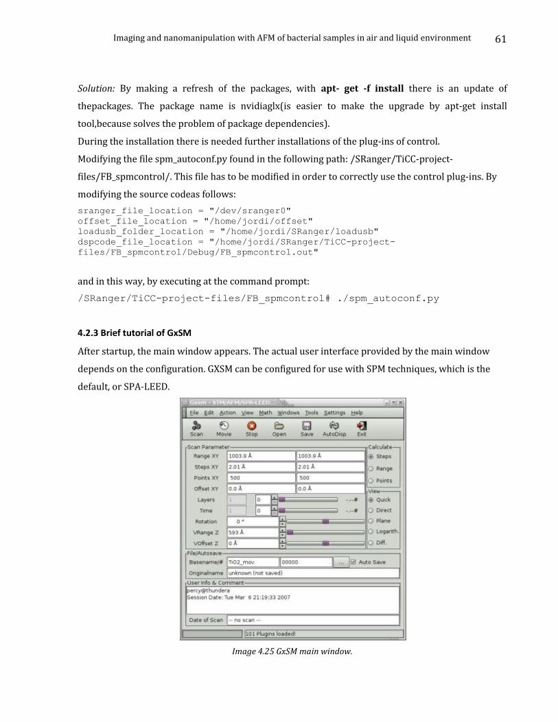
Imaging and nanomanipulation with AFM of bacterial samples in air and liquid environment
61
Solution: By making a refresh of the packages, with apt- get -f install there is an update of
thepackages. The package name is nvidiaglx(is easier to make the upgrade by apt-get install
tool,because solves the problem of package dependencies).
During the installation there is needed further installations of the plug-ins of control.
Modifying the file spm_autoconf.py found in the following path: /SRanger/TiCC-project-
files/FB_spmcontrol/. This file has to be modified in order to correctly use the control plug-ins. By
modifying the source codeas follows:
sranger_file_location = "/dev/sranger0"
offset_file_location = "/home/jordi/offset"
loadusb_folder_location = "/home/jordi/SRanger/loadusb"
dspcode_file_location = "/home/jordi/SRanger/TiCC-project-
files/FB_spmcontrol/Debug/FB_spmcontrol.out"
and in this way, by executing at the command prompt:
/SRanger/TiCC-project-files/FB_spmcontrol# ./spm_autoconf.py
4.2.3 Brief tutorial of GxSM
After startup, the main window appears. The actual user interface provided by the main window
depends on the configuration. GXSM can be configured for use with SPM techniques, which is the
default, or SPA-LEED.
Image 4.25 GxSM main window.
Imaging and nanomanipulation with AFM of bacterial samples in air and liquid environment
62
The main window provides two different functions: Firstly, it has a menu bar with pulldown menus.
These menus provide the user with the usual File and Help menus that can be found in practically
every mouse-driven software piece. Some of these pull-down menus interact with (Math) or start-
up (Windows) other windows. Secondly, the main menu contains a large number of control fields,
which can be used, e.g., to control an instrument, or just display certain parameters. These control
fields are described in the following two sections.
The main window contains from top to bottom the menubar, a taskbar, the scan parameter, view
mode, file, and info/comment sections, and a status and progress bar. The scan parameter and info
sections of the main window are used both for entering parameters during data taking and
displaying them after loading data.
Scan parameters: Each scan or image is characterized by its size and resolution. The size, or Range
XY, gives the scale of the image like the scale of a city map and denotes the height and width of the
scanned area. The resolution is determined by either the distance between the single scan
points/pixels given by Steps XY or the number of points in X and Y direction given by Points XY.
Given two of these parameters, the third one can be computed. The check box Calculate determines,
which of them is calculated by GXSM. For instance, if Steps is checked, a change of Range XY results
automatically in a new value for Steps XY.
The parameter Offset XY determines the distance of the zero-point of the image coordinates from
the center of the physical scanrange. The actual location of the zero-point within the scan depends
on the source of the data. If the data was acquired using GXSM, the zero-point is the middle of the
topmost line. Using Rotation, the imaged area can be rotated. Both inputs using numeric values and
the scrollbar are possible.
GXSM can be used to do spatially resolved spectroscopy (“probing”) measurements. Channels
containing probing data are essentially three-dimensional (3D) datasets. In these 3D datasets the X
and Y coordinates correspond to the 2D position like in conventional SPM images. The third
dimension, V, can contain spectroscopic information, such as I/V curves for scanning tunneling
spectroscopy. GXSM displays only one slice corresponding to one V value at a time. A layer denotes
the number of points in the V direction. Using Select, one of these slices corresponding to one V
value can be selected for visualization. VRange Z and VOffset Z are used for the visualization of the
scan data. They do not influence the data itself.
Problems faced with: During these months passed in installing the program, there have been spent a
lot a time in understanding the structure and hierarchy of the program. The impossibility to spend
more time in understanding it, have made us renounce.
Imaging and nanomanipulation with AFM of bacterial samples in air and liquid environment
63

Imaging and nanomanipulation with AFM of bacterial samples in air and liquid environment
64
Chapter 5: Nanobiocharacterization of Pseudomonas Au. and E. Coli with AFM pp.63
Chapter Index
5.5 First set of Experiments: Nanobiocharacterization of Pseudomonas au.and E. Coli pp.65
5.5.1 Pseudomonas Au pp.65 5.5.1.1 Characterization by Gram’s staining method pp.65 5.5.1.2 Characterization by optical microscopy pp.65 5.5.1.3 Topographical characterization using AFM pp.67 5.5.1.4 Mechanical characterization with AFM pp.70
5.5.2 Escherichia Coli pp.72 5.5.2.1 Characterization by Gram’s staining method pp.72 5.5.2.2 Characterization by optical microscopy pp.72 5.5.2.3 Topographical characterization using AFM pp.74 5.5.2.4 Mechanical characterization with AFM pp.81
5.5.3 Preliminary conclusions of the first set of experiments pp.81 5.6 Second set of Experiments: Nanobioch. of Pseudomonas over different substrates pp.82
5.6.1 Experiments pp.82 5.6.1.1 Characterization by non-AFM methods pp.82 5.6.1.2 Topographical characterization using AFM pp.82
5.6.2 Preliminary conclusions of the second set of experiments pp.84 5.7 Third set of Experiments: Nanobiocharacterization of Pseudomonas over gold pp.84
5.7.1 Preliminary results: Biofilm with cultivation time 20 hours pp.85 5.7.2 Preliminary results: Biofilm with cultivation time 24 hours pp.86 5.7.3 Preliminary results: Biofilm with cultivation time 28 hours pp.86 5.7.4 Preliminary results: Inoculated with cultivation time 28 hours pp.87
5.8 First experiments in liquid environment pp.88 5.8.1 Setting up the equipment pp.89
5.8.1.1 Imaging modes pp.89 5.8.1.2 Force curves pp.89
5.8.2 Experiments with biological samples pp.91 5.8.3 Preliminary conclusions of first set of experiments in liquid pp.94
Imaging and nanomanipulation with AFM of bacterial samples in air and liquid environment
65
In this chapter, I represent that part of work dedicated to scanning different biological samples over
different substrates. During these months there have been scanned three sets of samples, as are
presented in the index. They were gently prepared from Dr. Rosa Carmen Baños(Post doctoral
researcher at Institut de Bioenginyeria de Catalunya, IBEC). Bacteria like Escherichia Coli (E. Coli see
Appendix C) and Pseudomonas aeruginosa (Pseudomonas au. see Appendix C) were selected in base
of: their widespread in daily life (relevance as a pathogen), recognized as emerging opportunistic
pathogens of clinical relevance due to their increasing resistance to antibiotics (in isolated cases) as
recent studies [46] have noted persistence of E. Coli and Pseudomonas au. biofilms. (More over
biofilms, see Appendix A)
At first there is an optical phase, which helps to give an idea of bacterial aggregations and later
follows AFM mechanical and topographical characterization.
In this work is important to note that the whole is concluded with two main and satisfactory results:
1. Mechanical and topographical characterization of E. Coli and Pseudomonas au. biofilms,
especially of the links found between them.
2. Topographical characterization of biofilms in liquid environment.
The first one is of mayor importance as for our group and the one that we collaborate (Prof. Dr.
Antonio Juárez, Group Leader Biotecnologia microbiana i interacció hoste-patògen. IBEC) are the first
experiments making possible biofim characterization with AFM.
The second one is a big achievement for our group as the first time to characterize bacterial samples
in liquid environment. And more, we found once again links between bacteria, showing that liquid
imaging gives similar results to air imaging and establishes the basis for further dynamic studies of
bacteria’s in their habitat. Studies that give more realistic results, in comparison to the ones shown
here, as bacteria are fixed in the substrate.
Fixing bacteria implies, loosing information regarding bacteria-substrate surface adhesion forces. In
the sixth chapter we establish the basis for calculating these forces.
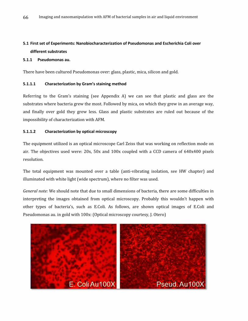
Imaging and nanomanipulation with AFM of bacterial samples in air and liquid environment
66
5.1 First set of Experiments: Nanobiocharacterization of Pseudomonas and Escherichia Coli over
different substrates
5.1.1 Pseudomonas au.
There have been cultured Pseudomonas over: glass, plastic, mica, silicon and gold.
5.1.1.1 Characterization by Gram’s staining method
Referring to the Gram’s staining (see Appendix A) we can see that plastic and glass are the
substrates where bacteria grew the most. Followed by mica, on which they grew in an average way,
and finally over gold they grew less. Glass and plastic substrates are ruled out because of the
impossibility of characterization with AFM.
5.1.1.2 Characterization by optical microscopy
The equipment utilized is an optical microscope Carl Zeiss that was working on reflection mode on
air. The objectives used were: 20x, 50x and 100x coupled with a CCD camera of 640x400 pixels
resolution.
The total equipment was mounted over a table (anti-vibrating isolation, see HW chapter) and
illuminated with white light (wide spectrum), where no filter was used.
General note: We should note that due to small dimensions of bacteria, there are some difficulties in
interpreting the images obtained from optical microscopy. Probably this wouldn’t happen with
other types of bacteria’s, such as E.Coli. As follows, are shown optical images of E.Coli and
Pseudomonas au. in gold with 100x: (Optical microscopy courtesy, J. Otero)
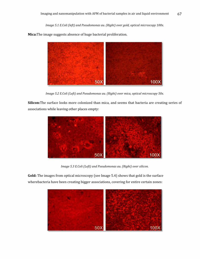
Imaging and nanomanipulation with AFM of bacterial samples in air and liquid environment
67
Image 5.1 E.Coli (left) and Pseudomonas au. (Right) over gold, optical microscopy 100x.
Mica:The image suggests absence of huge bacterial proliferation.
Image 5.2 E.Coli (Left) and Pseudomonas au. (Right) over mica, optical microscopy 50x.
Silicon:The surface looks more colonized than mica, and seems that bacteria are creating series of
associations while leaving other places empty:
Image 5.3 E.Coli (Left) and Pseudomonas au. (Right) over silicon.
Gold: The images from optical microscopy (see Image 5.4) shows that gold is the surface
wherebacteria have been creating bigger associations, covering for entire certain zones:
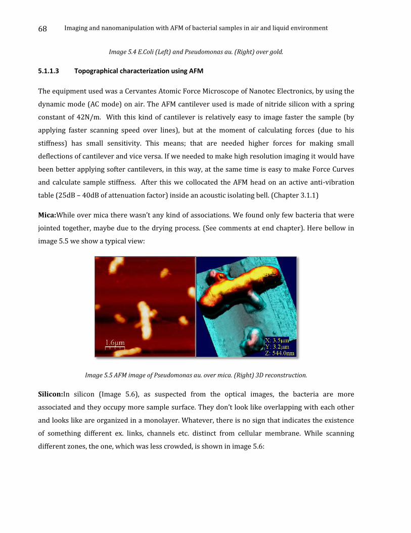
Imaging and nanomanipulation with AFM of bacterial samples in air and liquid environment
68
Image 5.4 E.Coli (Left) and Pseudomonas au. (Right) over gold.
5.1.1.3 Topographical characterization using AFM
The equipment used was a Cervantes Atomic Force Microscope of Nanotec Electronics, by using the
dynamic mode (AC mode) on air. The AFM cantilever used is made of nitride silicon with a spring
constant of 42N/m. With this kind of cantilever is relatively easy to image faster the sample (by
applying faster scanning speed over lines), but at the moment of calculating forces (due to his
stiffness) has small sensitivity. This means; that are needed higher forces for making small
deflections of cantilever and vice versa. If we needed to make high resolution imaging it would have
been better applying softer cantilevers, in this way, at the same time is easy to make Force Curves
and calculate sample stiffness. After this we collocated the AFM head on an active anti-vibration
table (25dB – 40dB of attenuation factor) inside an acoustic isolating bell. (Chapter 3.1.1)
Mica:While over mica there wasn’t any kind of associations. We found only few bacteria that were
jointed together, maybe due to the drying process. (See comments at end chapter). Here bellow in
image 5.5 we show a typical view:
Image 5.5 AFM image of Pseudomonas au. over mica. (Right) 3D reconstruction.
Silicon:In silicon (Image 5.6), as suspected from the optical images, the bacteria are more
associated and they occupy more sample surface. They don’t look like overlapping with each other
and looks like are organized in a monolayer. Whatever, there is no sign that indicates the existence
of something different ex. links, channels etc. distinct from cellular membrane. While scanning
different zones, the one, which was less crowded, is shown in image 5.6:
Imaging and nanomanipulation with AFM of bacterial samples in air and liquid environment
69
Image 5.6 AFM image of Pseudomonas au. over silicon.
For a better understanding of this region, we liked to make further zooms and a line of profile over
few bacteria as is shown in Image 5.7:
Image 5.7 3D profiling of a previous section of Pseudomonas. (Left) Profile of the line visible in 3D reconstruction.
Gold:The substrate, as we can see from the optical images in image 5.1, is covered with bacteria. We
can definitely say that here bacteria form a monolayer, as in general they aren’t deposed one upon
the others forming higher aggregations.
Imaging and nanomanipulation with AFM of bacterial samples in air and liquid environment
70
Image 5.8 Pseudomonas au. over gold. (Left) In circles are evidenced interconnections between bacteria. (Right)
3D reconstruction of zone of interest.
Remarkable is the appearance of interconnections (normally simples, and sometimes doubles)
between bacteria (but not in general, only between few of them). Links with dimensions of about
100nm in height and 200nm in width:
Image 5.9 Pseudomonas over gold. Zoom in over interconnections. (Left) Profiling of double interconnections
between two Pseudomonas. (Right) 3D reconstruction.
Imaging and nanomanipulation with AFM of bacterial samples in air and liquid environment
71
5.1.1.4 Mechanical characterization with AFM
The links appeared in the images seems to be specific and different from the bacterial membrane.
For demonstrating this, it’s important to make some mechanical test over them (Force Vs
Displacement curves) in order to compare with tests made over bacteria membranes.
We used the same AFM microscope as in the topographical characterization measurements, but
with a cantilever that has higher resolution when making mechanical tests. This implies using a
cantilever with smaller spring constant k (we used Olympus cantilevers)
More in detail, it was a cantilever made of silicon nitride with spring constant around 0.76 N/m. The
images, previous to mechanical tests (essential for localizing the working points) were made in air
using dynamical mode. This kind of cantilever isn’t the proper one for these requirements, but
working slowly (40min/image) and leaving the whole system stabilizing (round 1-2 days), is
possible to get images of similar quality than the previous ones. And here bellow in Image 5.10 is
shown the result of the choices made at the time when to image the sample:
Image 5.10 Pseudomonas au. over gold.
Later there have been tests (force curves: force vs. displacement):
20 force curves over the “channel”.
20 force curves over the central part of bacteria.
Imaging and nanomanipulation with AFM of bacterial samples in air and liquid environment
72
Image 5.11 Force curves over channel between two Pseudomonas and over membrane.
From the analysis of the average 20 curves (Image 5.11) there is a clear difference between channel
composition and bacterial membrane composition. We can see more adhesion (need of 8nN force to
unhook from the “channel” in comparison of the 6nN to uncouple from the membrane).
At the same time if we focus on the graph at bottom left in image 5.11, there are slope differences
between forward (green) and backward (red) curves. In this way bridges presents’ higher
viscoelastic behaviour than membranes, which in turn presents more elastic behaviour.
For each displacement in one of the curves at the contact zone (slope part of FZ graph), let’s say -20
nm, the applied force over the bacteria almost doubles the force over the channel. This shows that
the channel is more easily deformable (for same Z movements, the channel sinks more, so the
cantilever deflexion is smaller), having smaller elastic module (softer material).
We should note the necessity of a calibration process of the whole AFM, regarding the photodiode
calibration, piezo calibration, and at the end comparison of these slopes with a slope over sample
surface where aren’t present membranes. This further step will permit us to compare different
slopes between membrane and rigid surface.
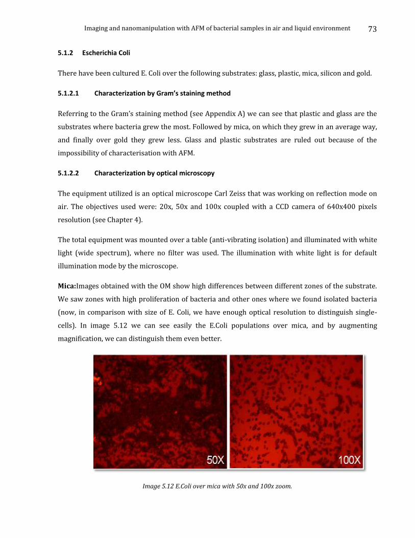
Imaging and nanomanipulation with AFM of bacterial samples in air and liquid environment
73
5.1.2 Escherichia Coli
There have been cultured E. Coli over the following substrates: glass, plastic, mica, silicon and gold.
5.1.2.1 Characterization by Gram’s staining method
Referring to the Gram’s staining method (see Appendix A) we can see that plastic and glass are the
substrates where bacteria grew the most. Followed by mica, on which they grew in an average way,
and finally over gold they grew less. Glass and plastic substrates are ruled out because of the
impossibility of characterisation with AFM.
5.1.2.2 Characterization by optical microscopy
The equipment utilized is an optical microscope Carl Zeiss that was working on reflection mode on
air. The objectives used were: 20x, 50x and 100x coupled with a CCD camera of 640x400 pixels
resolution (see Chapter 4).
The total equipment was mounted over a table (anti-vibrating isolation) and illuminated with white
light (wide spectrum), where no filter was used. The illumination with white light is for default
illumination mode by the microscope.
Mica:Images obtained with the OM show high differences between different zones of the substrate.
We saw zones with high proliferation of bacteria and other ones where we found isolated bacteria
(now, in comparison with size of E. Coli, we have enough optical resolution to distinguish single-
cells). In image 5.12 we can see easily the E.Coli populations over mica, and by augmenting
magnification, we can distinguish them even better.
Image 5.12 E.Coli over mica with 50x and 100x zoom.
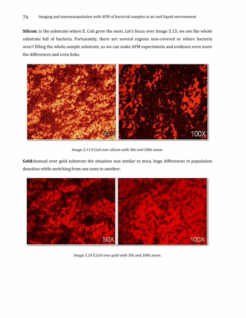
Imaging and nanomanipulation with AFM of bacterial samples in air and liquid environment
74
Silicon: is the substrate where E. Coli grew the most. Let’s focus over Image 5.13; we see the whole
substrate full of bacteria. Fortunately, there are several regions non-covered or where bacteria
aren’t filling the whole sample substrate, so we can make AFM experiments and evidence even more
the differences and even links.
Image 5.13 E.Coli over silicon with 50x and 100x zoom.
Gold:Instead over gold substrate the situation was similar to mica, huge differences in population
densities while switching from one zone to another:
Image 5.14 E.Coli over gold with 50x and 100x zoom.
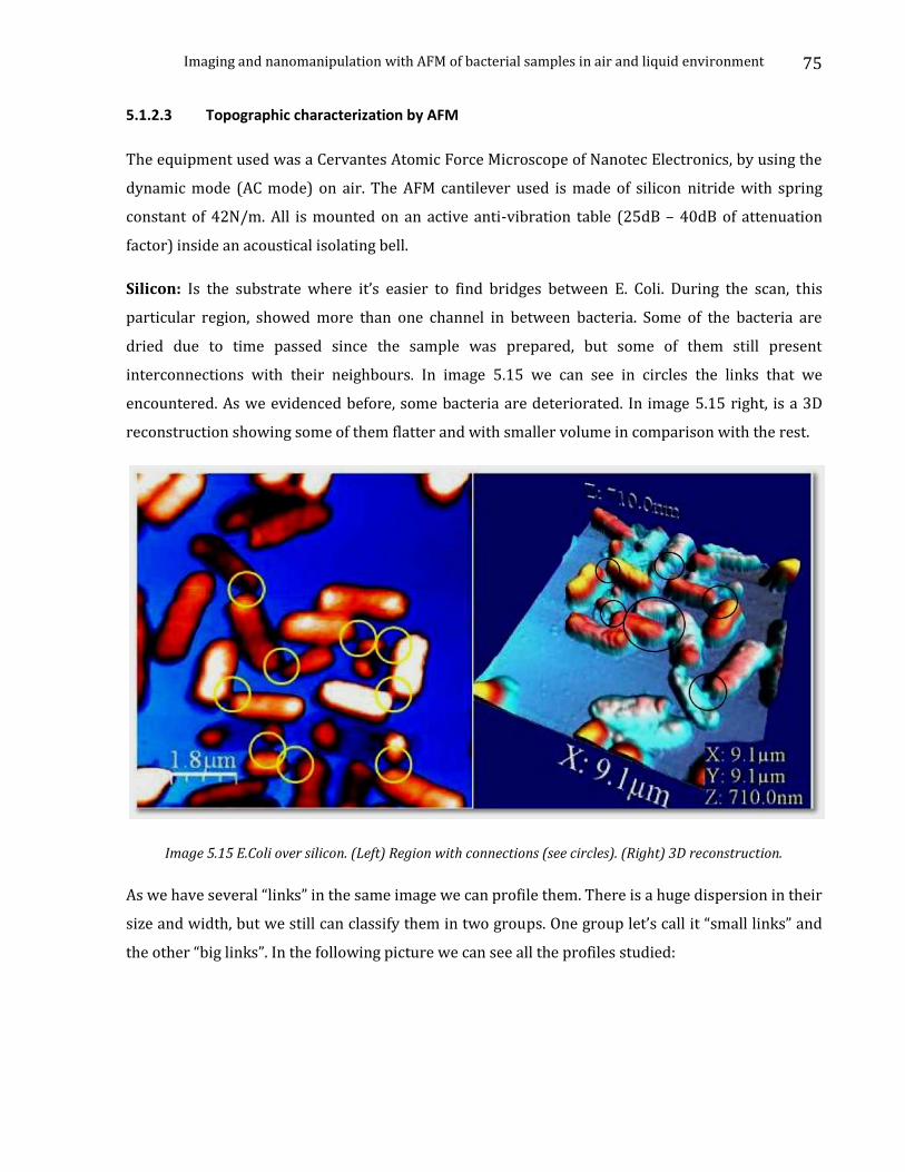
Imaging and nanomanipulation with AFM of bacterial samples in air and liquid environment
75
5.1.2.3 Topographic characterization by AFM
The equipment used was a Cervantes Atomic Force Microscope of Nanotec Electronics, by using the
dynamic mode (AC mode) on air. The AFM cantilever used is made of silicon nitride with spring
constant of 42N/m. All is mounted on an active anti-vibration table (25dB – 40dB of attenuation
factor) inside an acoustical isolating bell.
Silicon: Is the substrate where it’s easier to find bridges between E. Coli. During the scan, this
particular region, showed more than one channel in between bacteria. Some of the bacteria are
dried due to time passed since the sample was prepared, but some of them still present
interconnections with their neighbours. In image 5.15 we can see in circles the links that we
encountered. As we evidenced before, some bacteria are deteriorated. In image 5.15 right, is a 3D
reconstruction showing some of them flatter and with smaller volume in comparison with the rest.
Image 5.15 E.Coli over silicon. (Left) Region with connections (see circles). (Right) 3D reconstruction.
As we have several “links” in the same image we can profile them. There is a huge dispersion in their
size and width, but we still can classify them in two groups. One group let’s call it “small links” and
the other “big links”. In the following picture we can see all the profiles studied:
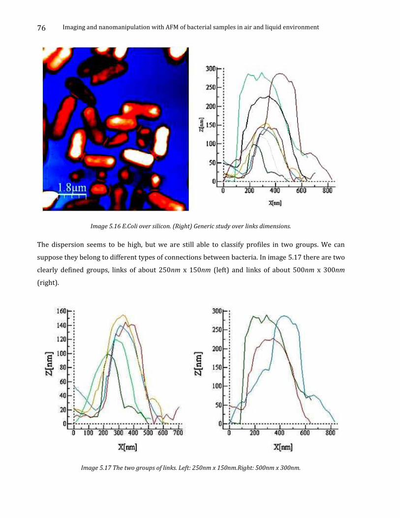
Imaging and nanomanipulation with AFM of bacterial samples in air and liquid environment
76
Image 5.16 E.Coli over silicon. (Right) Generic study over links dimensions.
The dispersion seems to be high, but we are still able to classify profiles in two groups. We can
suppose they belong to different types of connections between bacteria. In image 5.17 there are two
clearly defined groups, links of about 250nm x 150nm (left) and links of about 500nm x 300nm
(right).
Image 5.17 The two groups of links. Left: 250nm x 150nm.Right: 500nm x 300nm.
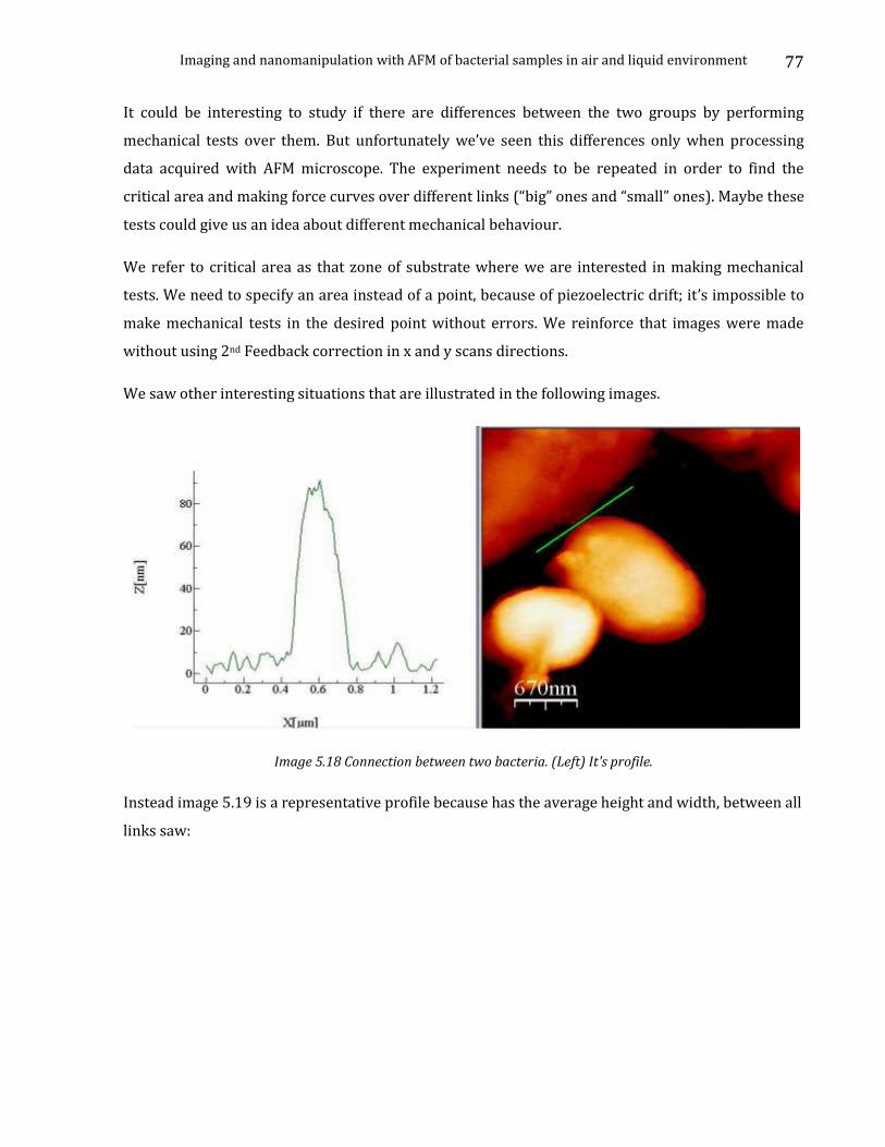
Imaging and nanomanipulation with AFM of bacterial samples in air and liquid environment
77
It could be interesting to study if there are differences between the two groups by performing
mechanical tests over them. But unfortunately we’ve seen this differences only when processing
data acquired with AFM microscope. The experiment needs to be repeated in order to find the
critical area and making force curves over different links (“big” ones and “small” ones). Maybe these
tests could give us an idea about different mechanical behaviour.
We refer to critical area as that zone of substrate where we are interested in making mechanical
tests. We need to specify an area instead of a point, because of piezoelectric drift; it’s impossible to
make mechanical tests in the desired point without errors. We reinforce that images were made
without using 2nd Feedback correction in x and y scans directions.
We saw other interesting situations that are illustrated in the following images.
Image 5.18 Connection between two bacteria. (Left) It's profile.
Instead image 5.19 is a representative profile because has the average height and width, between all
links saw:

Imaging and nanomanipulation with AFM of bacterial samples in air and liquid environment
78
Image 5.19 Representative link. (Left) It's profile.
While in image 5.20 we had the border effects probably due to drift problems or because we didn’t
control in the right way set point, scan speed and feedback values.
Image 5.20 Interesting link between two E.Coli. (Left) It's profile.
Further zoom in and 3D reconstruction of this link is shown in image 5.21.
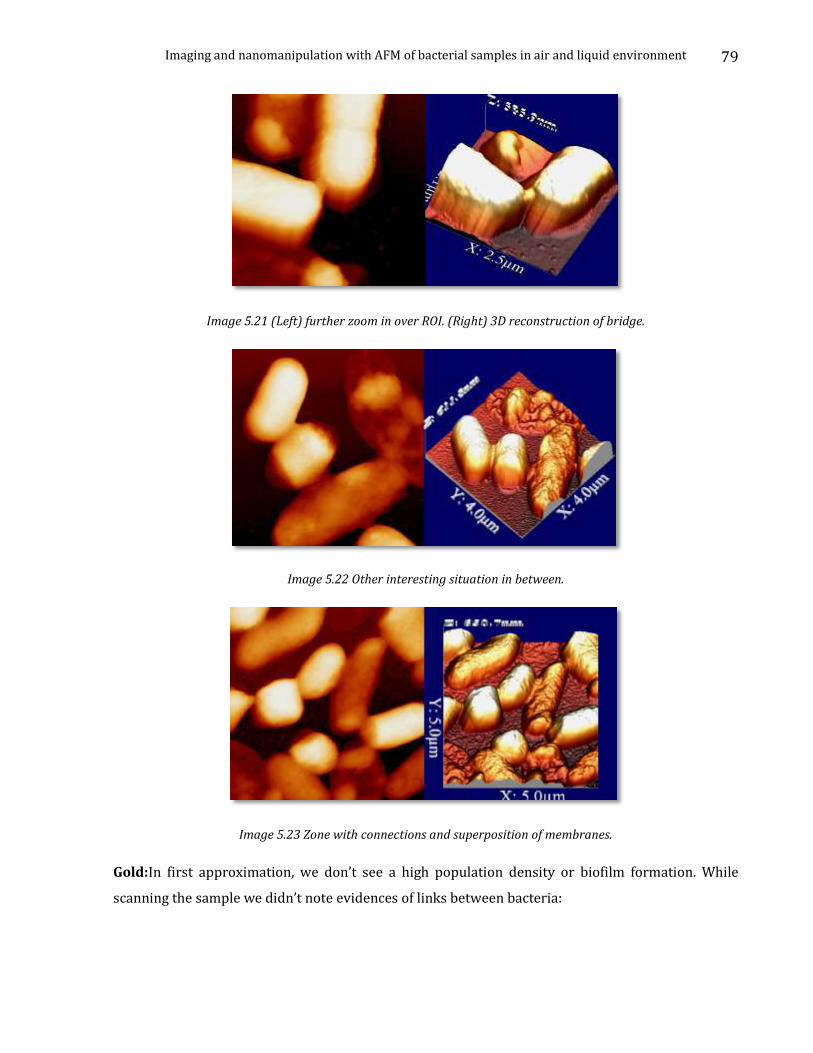
Imaging and nanomanipulation with AFM of bacterial samples in air and liquid environment
79
Image 5.21 (Left) further zoom in over ROI. (Right) 3D reconstruction of bridge.
Image 5.22 Other interesting situation in between.
Image 5.23 Zone with connections and superposition of membranes.
Gold:In first approximation, we don’t see a high population density or biofilm formation. While
scanning the sample we didn’t note evidences of links between bacteria:
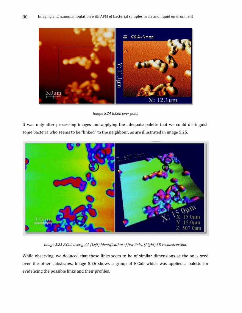
Imaging and nanomanipulation with AFM of bacterial samples in air and liquid environment
80
Image 5.24 E.Coli over gold.
It was only after processing images and applying the adequate palette that we could distinguish
some bacteria who seems to be “linked” to the neighbour, as are illustrated in image 5.25.
Image 5.25 E.Coli over gold. (Left) Identification of few links. (Right) 3D reconstruction.
While observing, we deduced that these links seem to be of similar dimensions as the ones seed
over the other substrates. Image 5.26 shows a group of E.Coli which was applied a palette for
evidencing the possible links and their profiles.

Imaging and nanomanipulation with AFM of bacterial samples in air and liquid environment
81
Image 5.26 E.Coli over gold. (Right) Profiling of selected links.
Mica: Here we found similar situation that over gold substrate. There aren’t much links or bacterial
structures that are different from simply two bacterial membranes attached together because of
being closer to each other. In image 5.27 are shown some bacteria that possibly have created biofim.
Image 5.27 E.Coli over mica. (Right) 3D reconstruction.
Image 5.28 Link of “big” dimensions. Image 5.29 Link of “small” dimensions.

Imaging and nanomanipulation with AFM of bacterial samples in air and liquid environment
82
5.1.2.4 Mechanical characterization with AFM
Due to few problems and mistakes in the procedure followed, the results of mechanical tests over E.
Coli’s links aren’t valid. This because it was difficult to find these links between E. Coli when using a
cantilever with enough sensitivity (“softer” cantilever) to perform these tests, we decide not to
repeat them and leave this study for the near future.
A “softer” cantilever implies smaller k values (Olympus SiN, k=0.76 N/m); this means there are
needed smaller force values to bend. Implying smaller forces exerted over substrate. But at the same
time introduces more noise and is difficult to distinguish between real obstacles (bacterial
membranes) and fictitious obstacles (noise). Typical artefacts when of using softer cantilevers are:
False engages. At approach time, while getting closer to substrate with motors due to higer
deflections of cantilever for small displacements; is easy to get a false engage. The
“sensation” of overcoming the percentual cantilever deflection ranges that we consider
approach (See for more in detail use of approach tool in chapter 4.1.3).
Blurried images. Where from the topography backward and forward channels they seem
like following each other, but the real situation is: cantilever floating over the surface. This is
more evidences when makin FZ curves over the substrate; cantilever “feels” the surface
much before we have real contact with surface. This efect is more evidenced when there is
presence of ionic double layer (See chapter 4.1.6).
5.1.3 Preliminary conclusions of the first set of experiments
Is possible that the results over mica could be erroneous because it seems there were few
problems at the moment of separation from the culture due to exfoliation. In future studies
of E.Coli's behaviour, it should be taken in consideration.
The tests were made in the following order: mica, silicon and gold. Without previous
experience in imaging pseudomonas with AFM, we consider that the ones taken in gold are
the best. This because in gold we saw the connections perfectly this doesn't discard the
possibility of other substrates.
In case is needed more information over the material (Young module, etc.), experiments
should be repeated in nitrogen ambient or liquid. Air results are important and can serve us
in making compared analysis, “fast one”, an can be the principle for detecting differences
between those materials.
We choose to follow with a second set of experiments only with pseudomonas over different
substrates.
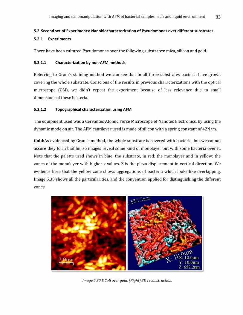
Imaging and nanomanipulation with AFM of bacterial samples in air and liquid environment
83
5.2 Second set of Experiments: Nanobiocharacterization of Pseudomonas over different substrates
5.2.1 Experiments
There have been cultured Pseudomonas over the following substrates: mica, silicon and gold.
5.2.1.1 Characterization by non-AFM methods
Referring to Gram’s staining method we can see that in all three substrates bacteria have grown
covering the whole substrate. Conscious of the results in previous characterizations with the optical
microscope (OM), we didn’t repeat the experiment because of less relevance due to small
dimensions of these bacteria.
5.2.1.2 Topographical characterization using AFM
The equipment used was a Cervantes Atomic Force Microscope of Nanotec Electronics, by using the
dynamic mode on air. The AFM cantilever used is made of silicon with a spring constant of 42N/m.
Gold:As evidenced by Gram’s method, the whole substrate is covered with bacteria, but we cannot
assure they form biofilm, so images reveal some kind of monolayer but with some bacteria over it.
Note that the palette used shows in blue: the substrate, in red: the monolayer and in yellow: the
zones of the monolayer with higher z values. Z is the piezo displacement in vertical direction. We
evidence here that the yellow zone shows aggregations of bacteria which looks like overlapping.
Image 5.30 shows all the particularities, and the convention applied for distinguishing the different
zones.
Image 5.30 E.Coli over gold. (Right) 3D reconstruction.
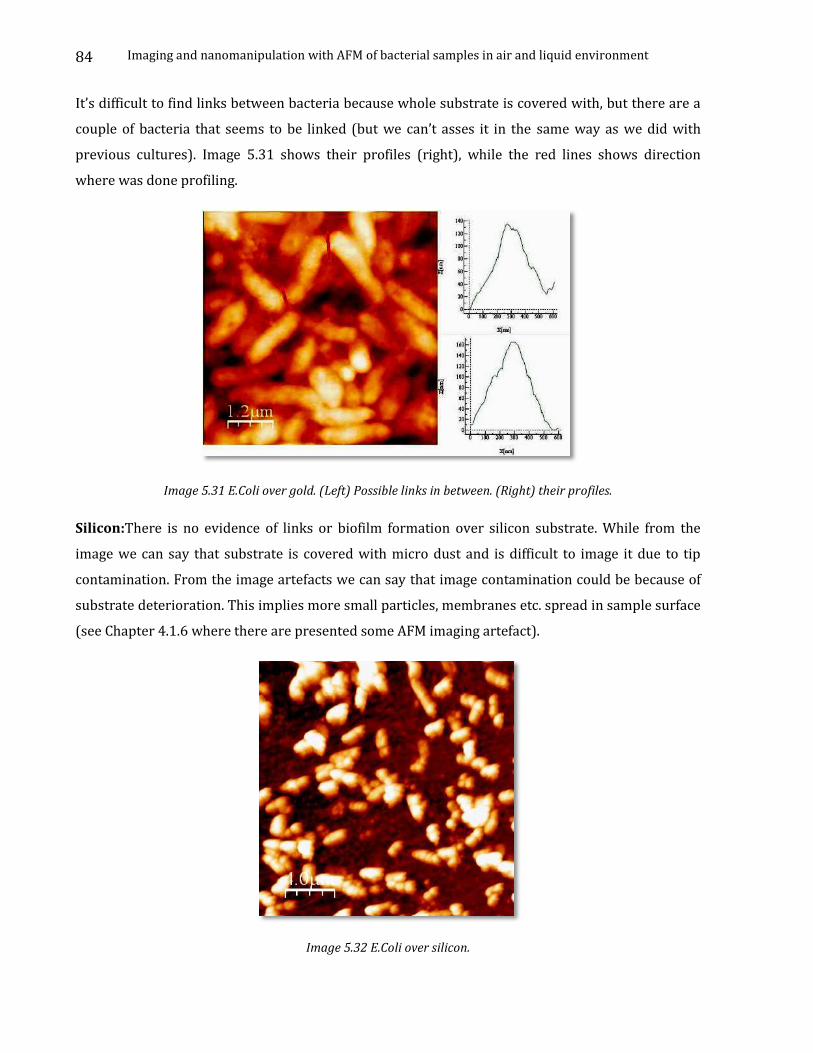
Imaging and nanomanipulation with AFM of bacterial samples in air and liquid environment
84
It’s difficult to find links between bacteria because whole substrate is covered with, but there are a
couple of bacteria that seems to be linked (but we can’t asses it in the same way as we did with
previous cultures). Image 5.31 shows their profiles (right), while the red lines shows direction
where was done profiling.
Image 5.31 E.Coli over gold. (Left) Possible links in between. (Right) their profiles.
Silicon:There is no evidence of links or biofilm formation over silicon substrate. While from the
image we can say that substrate is covered with micro dust and is difficult to image it due to tip
contamination. From the image artefacts we can say that image contamination could be because of
substrate deterioration. This implies more small particles, membranes etc. spread in sample surface
(see Chapter 4.1.6 where there are presented some AFM imaging artefact).
Image 5.32 E.Coli over silicon.

Imaging and nanomanipulation with AFM of bacterial samples in air and liquid environment
85
Mica:Bacteria seem to occupy whole mica substrate and they look like forming monolayer. But due
to high population density of substrate, we’re not able to find bridges between them. Is interesting
to note that the relief is rougher and this is an index of les monolayer creation. More in specific, a
monolayer looks like more planar and this one isn’t so planar.
Image 5.33 E. Coli over mica. Image 5.34 Its 3D reconstruction.
5.2.2 Preliminary conclusions of second set of experiments
Bacteria have occupied the whole substrate and it increases the difficulty of experiments.
Samples seem to be quite different from the ones of the first set of experiments.
This second set of experiments may confirm gold as the proper one for further experiments.
5.3 Third set of Experiments: Nanobiocharacterization of Pseudomonas over gold
In this third set of experiments we used the following samples:
Pseudomonas over gold substrate forming biofilm. There have been prepared three sets of Petri
dishes with cultivation time corresponding to: 20,24 and 28 hours.
Inoculated bacteria of same cultures (in 20, 24 and 28h) dropped and dried over gold, without
further treatments.
We didn’t pass through Gram’s method and optical characterization phase as we did in previous
sections. The main reasons were: firstly, for getting fresh cultivations directly under observation.
And secondly, because membrane properties and biofilm formation depends on time, we wanted to
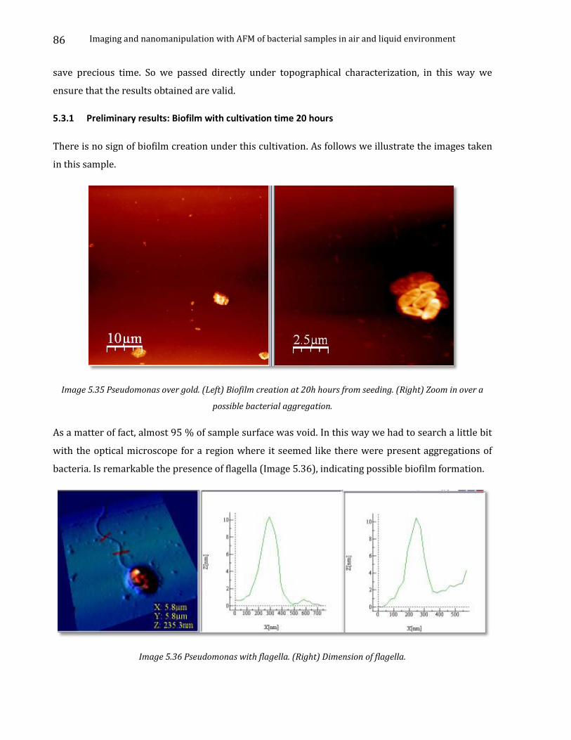
Imaging and nanomanipulation with AFM of bacterial samples in air and liquid environment
86
save precious time. So we passed directly under topographical characterization, in this way we
ensure that the results obtained are valid.
5.3.1 Preliminary results: Biofilm with cultivation time 20 hours
There is no sign of biofilm creation under this cultivation. As follows we illustrate the images taken
in this sample.
Image 5.35 Pseudomonas over gold. (Left) Biofilm creation at 20h hours from seeding. (Right) Zoom in over a
possible bacterial aggregation.
As a matter of fact, almost 95 % of sample surface was void. In this way we had to search a little bit
with the optical microscope for a region where it seemed like there were present aggregations of
bacteria. Is remarkable the presence of flagella (Image 5.36), indicating possible biofilm formation.
Image 5.36 Pseudomonas with flagella. (Right) Dimension of flagella.
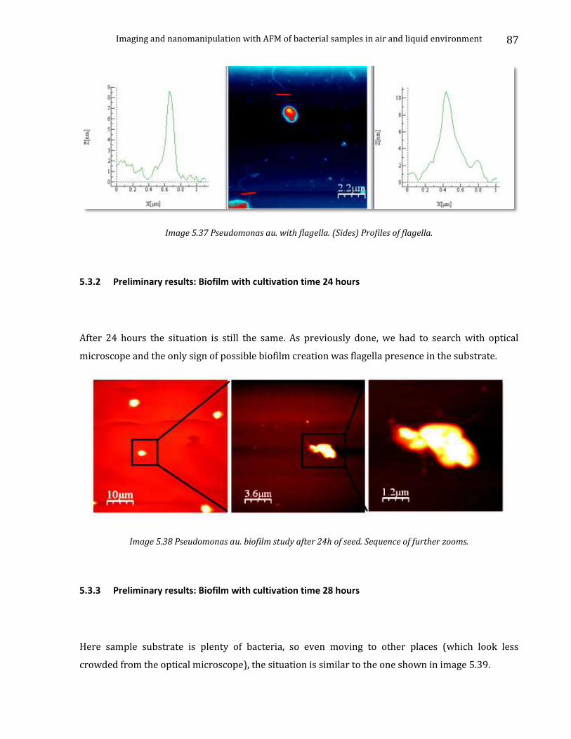
Imaging and nanomanipulation with AFM of bacterial samples in air and liquid environment
87
Image 5.37 Pseudomonas au. with flagella. (Sides) Profiles of flagella.
5.3.2 Preliminary results: Biofilm with cultivation time 24 hours
After 24 hours the situation is still the same. As previously done, we had to search with optical
microscope and the only sign of possible biofilm creation was flagella presence in the substrate.
Image 5.38 Pseudomonas au. biofilm study after 24h of seed. Sequence of further zooms.
5.3.3 Preliminary results: Biofilm with cultivation time 28 hours
Here sample substrate is plenty of bacteria, so even moving to other places (which look less
crowded from the optical microscope), the situation is similar to the one shown in image 5.39.
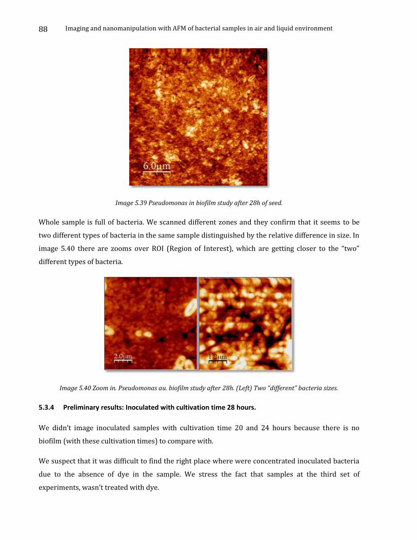
Imaging and nanomanipulation with AFM of bacterial samples in air and liquid environment
88
Image 5.39 Pseudomonas in biofilm study after 28h of seed.
Whole sample is full of bacteria. We scanned different zones and they confirm that it seems to be
two different types of bacteria in the same sample distinguished by the relative difference in size. In
image 5.40 there are zooms over ROI (Region of Interest), which are getting closer to the “two”
different types of bacteria.
Image 5.40 Zoom in. Pseudomonas au. biofilm study after 28h. (Left) Two “different” bacteria sizes.
5.3.4 Preliminary results: Inoculated with cultivation time 28 hours.
We didn’t image inoculated samples with cultivation time 20 and 24 hours because there is no
biofilm (with these cultivation times) to compare with.
We suspect that it was difficult to find the right place where were concentrated inoculated bacteria
due to the absence of dye in the sample. We stress the fact that samples at the third set of
experiments, wasn’t treated with dye.
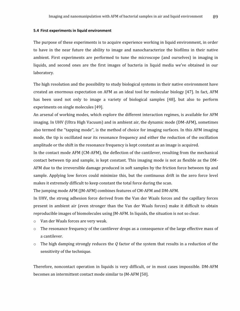
Imaging and nanomanipulation with AFM of bacterial samples in air and liquid environment
89
5.4 First experiments in liquid environment
The purpose of these experiments is to acquire experience working in liquid environment, in order
to have in the near future the ability to image and nanocharacterize the biofilms in their native
ambient. First experiments are performed to tune the microscope (and ourselves) in imaging in
liquids, and second ones are the first images of bacteria in liquid media we’ve obtained in our
laboratory.
The high resolution and the possibility to study biological systems in their native environment have
created an enormous expectation on AFM as an ideal tool for molecular biology [47]. In fact, AFM
has been used not only to image a variety of biological samples [48], but also to perform
experiments on single molecules [49].
An arsenal of working modes, which explore the different interaction regimes, is available for AFM
imaging. In UHV (Ultra High Vacuum) and in ambient air, the dynamic mode (DM-AFM), sometimes
also termed the ‘‘tapping mode’’, is the method of choice for imaging surfaces. In this AFM imaging
mode, the tip is oscillated near its resonance frequency and either the reduction of the oscillation
amplitude or the shift in the resonance frequency is kept constant as an image is acquired.
In the contact mode AFM (CM-AFM), the deflection of the cantilever, resulting from the mechanical
contact between tip and sample, is kept constant. This imaging mode is not as flexible as the DM-
AFM due to the irreversible damage produced in soft samples by the friction force between tip and
sample. Applying low forces could minimize this, but the continuous drift in the zero force level
makes it extremely difficult to keep constant the total force during the scan.
The jumping mode AFM (JM-AFM) combines features of CM-AFM and DM-AFM.
In UHV, the strong adhesion force derived from the Van der Waals forces and the capillary forces
present in ambient air (even stronger than the Van der Waals forces) make it difficult to obtain
reproducible images of biomolecules using JM-AFM. In liquids, the situation is not so clear.
o Van der Waals forces are very weak.
o The resonance frequency of the cantilever drops as a consequence of the large effective mass of
a cantilever.
o The high damping strongly reduces the Q factor of the system that results in a reduction of the
sensitivity of the technique.
Therefore, noncontact operation in liquids is very difficult, or in most cases impossible. DM-AFM
becomes an intermittent contact mode similar to JM-AFM [50].

Imaging and nanomanipulation with AFM of bacterial samples in air and liquid environment
90
In liquids, the most appropriate imaging mode depends on the sample characteristics and
preparation methods [51]. Contact or dynamic modes are the best choices for imaging molecular
assemblies arranged as crystals such as the purple membrane. In this case, the advantage of image
acquisition speed predominates over the disadvantage of high lateral or normal force. For imaging
individual macromolecules, which are weakly bonded to the substrate, lateral and normal forces are
the relevant factors, and hence the jumping mode, an imaging mode that minimizes lateral and
normal forces, is preferable to other imaging modes.
5.4.1 Setting up the equipment
5.4.1.1 Imaging modes
There are three different imaging modes in which AFM can work in liquid environment: dynamic
(AC mode, oscillating the cantilever), contact (DC mode, constant force over the sample) and
jumping (JM mode, approaching and withdrawing the tip from the sample in different points and
calculating the contact point). We use a grid (PMMA) of known geometry to set up the system, and
after obtaining optimal parameters for the imaging settings we obtain images in the three modes:
Image 5.41 Grid scanned from left to right in: Contact, Dynamic and Jumping.
5.4.1.2 Force curves
The experiments in liquid require controlling the pH. Due to ionic double layer forces the tip “feels”
surface at long distances. While hydrophobic forces attract water molecules to the tip increasing it’s
effective radius (and consequently the convolution surface) increases, decreasing resolution. Image
5.41 represents generic force curves when working in distilled water. Let’s note that we start feeling
substrate since 1 m far from surface. This is visible in the graph because the forces are different
from zero. We would like to add that normal ranges of contact distance in AC mode are definitely
smaller than this one.
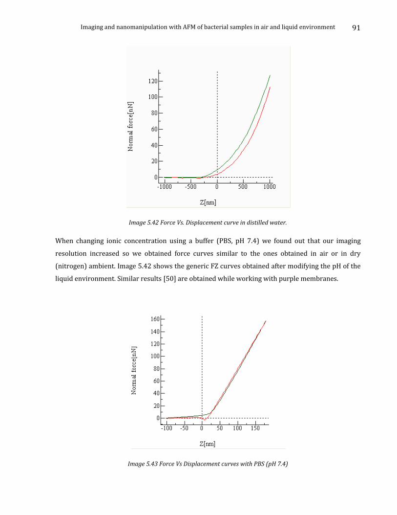
Imaging and nanomanipulation with AFM of bacterial samples in air and liquid environment
91
Image 5.42 Force Vs. Displacement curve in distilled water.
When changing ionic concentration using a buffer (PBS, pH 7.4) we found out that our imaging
resolution increased so we obtained force curves similar to the ones obtained in air or in dry
(nitrogen) ambient. Image 5.42 shows the generic FZ curves obtained after modifying the pH of the
liquid environment. Similar results [50] are obtained while working with purple membranes.
Image 5.43 Force Vs Displacement curves with PBS (pH 7.4)
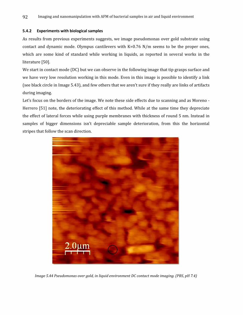
Imaging and nanomanipulation with AFM of bacterial samples in air and liquid environment
92
5.4.2 Experiments with biological samples
As results from previous experiments suggests, we image pseudomonas over gold substrate using
contact and dynamic mode. Olympus cantilevers with K=0.76 N/m seems to be the proper ones,
which are some kind of standard while working in liquids, as reported in several works in the
literature [50].
We start in contact mode (DC) but we can observe in the following image that tip grasps surface and
we have very low resolution working in this mode. Even in this image is possible to identify a link
(see black circle in Image 5.43), and few others that we aren’t sure if they really are links of artifacts
during imaging.
Let’s focus on the borders of the image. We note these side effects due to scanning and as Moreno -
Herrero [51] note, the deteriorating effect of this method. While at the same time they depreciate
the effect of lateral forces while using purple membranes with thickness of round 5 nm. Instead in
samples of bigger dimensions isn’t depreciable sample deterioration, from this the horizontal
stripes that follow the scan direction.
Image 5.44 Pseudomonas over gold, in liquid environment DC contact mode imaging. (PBS, pH 7.4)

Imaging and nanomanipulation with AFM of bacterial samples in air and liquid environment
93
In a second intent, we tried to image the sample in AC mode (Tapping) and achieved getting higher
resolution in comparison with DC mode. Bellow we show the results obtained (see black circles in
Image 5.45). While scanning sample we had to apply slower scan speed (time for scanning one
single line). Then we change to dynamic mode and we can see more clearly the sample, and even
distinguish some (Image 5.44) links between bacteria:
Image 5.45 Pseudomonas au. over gold. AC mode, in circles are evidenced the links found in the sample.

Imaging and nanomanipulation with AFM of bacterial samples in air and liquid environment
94
Image 5.46 Pseudomonas over gold in tapping mode. Evidence of links (circle left). 3D reconstruction (right).
While zooming and profiling, effectively it looks similar to the ones found in air:
Image 5.47 Zone of interest. (Left) Link profile. (Right) Link.
Imaging and nanomanipulation with AFM of bacterial samples in air and liquid environment
95
5.4.3 Preliminary conclusions of first set of experiments in liquid
Biofilm imaging in liquid with the AFM is possible, so we’re working in the proper direction
towards “living cells studies”.
Experimental results give us a starting point to continue:
o Using a pH 7.4 with normal PBS
o Softer cantilevers k=0.7 N/m or less
o Over gold substrate
o Better with pseudomonas
Due to the time spent for imaging only one substrate (several days for one sample), we focused
more over gold especially with one sample/cultivation. The sample choice is of high importance
in the near future.
More tests are required, for a better performance in imaging procedure and in sample
“construction”.
Imaging and nanomanipulation with AFM of bacterial samples in air and liquid environment
96
Chapter 6: Lithography and tip movement automation pp.95
Chapter Index
6.4 Short Introduction in Lithography pp.96 6.5 Lithography language pp.99 6.6 Automation of probe movements pp.103
6.6.1 Making Force Vs Displacement curves in a determined point pp.104 6.6.2 Multiple Force Vs Displacement curves in a line and in a matrix pp.106 6.6.3 Modifying sample surface in Lithography mode pp.107
6.6.3.1 Experiment: Breaking bacteria pp.112 6.6.3.2 Experiment: Moving bacteria pp.114 6.6.3.3 Experiment: Breaking bacteria’s membrane pp.116 6.6.3.4 Experiment: Breaking through a bacteria pp.118 6.6.3.5 Experiment: Force measurement while breaking a link with probe pp.119 6.6.3.6 Experiment: Force measurement while moving bacteria pp.122
Imaging and nanomanipulation with AFM of bacterial samples in air and liquid environment
97
During previous chapters we have seen AFM as a microscope, a really good instrument for making
good imaging, but the reality is that that’s not enough. While thinking over the microscope
construction, is easy to think that the tip can be used booth for imaging and even as a
nanomanipulating tool.
In this way the same tip does imaging and manipulation sections. And one of these processes is the
automation of tip movement.
By tip movement automations we mean the joint of different small built-in movements for achieving
a bigger and more complex tip movement. These built-ins are defined by microscope constructors
and we can se them as the universe of discussion, as the whole “AFM dictionary”, and by these
“words” that we can build more complex and meaningful “sentences”.
This metaphor explains and describes a little bit the limitations in movement and automation
complexity imposed by these built-ins, because there is always dependence by the given dictionary.
And in the following paragraphs will be showed how we achieved solving these limitations.
6.1 Short Introduction in Lithography
Lithography is a part of the WSxM program. In this frame is possible to draw on a sample, define the
tip motion and write on a sample (More exhaustive in Appendix B)
WSxM Lithography section allows moving the tip over the sample performing different actions. We
can think in the tip as a pen, and the sample as a paper. If we can somehow define what does “draw”
mean, we can “draw” with our tip over the sample, as it was a pen.
And vice versa, if the pen point is far away from the paper surface, it will draw nothing. In a
symmetric way it can be done with WSxM Lithography if is defined previously what “do not draw”
means in our tip-sample system.
In this way there is the possibility to decide what “draw” stands for and what “do not draw” stands
for.But we still need another concept; move. So we can make a workflow describing how it works
lithography.
Here “draw” can be at the same time a single one instruction or a set of instructions that compose
the complex concept of draw.To explain it better we can illustrate some examples of what a draw
instruction can be.
Imaging and nanomanipulation with AFM of bacterial samples in air and liquid environment
98
Oxidation process
In our equipment is possible to apply a voltage between tip and sample without contact
between them. These voltage differences induce surface oxidation, a process that deposit a
layer of samples oxide due to electron exchanges occurring bellow the tip.
Nanotec Electrónica S.L developers have made oxidation experiments.
In the Image 6.1 was induced a bias voltage between tip and silicon surface following a
pattern. These images are 3D reconstructions of the topographical images. The relief is
obtained by SiO2 deposition over Si substrate. Here the tip moves with voltage applied over
the surface following patterns already established in the lithography section.
So, the “Draw process” here is: Set Bias voltages between tip and sample. In this way the
previous flow diagram can be specified like this:
Image 6.1 (Left) Logo Nanotec 1um x 1um. (Right) Don Quijote and Sancho 1.3um x 1.3um.
Surface modification process.
Surface modifications can be obtained as a collection of more than one “Draw Instructions” like:
Zmove, Line, DoRamp…etc. These kind of manipulations will be the aim of my work in the
following chapter, and will be explained more carefully.
If we take a closer look to WSxM diagram, it could be represented with the diagram of Image 6.2.
There are three main sub-trees:
Data acquisition.
Lithography.
Data processing.
Imaging and nanomanipulation with AFM of bacterial samples in air and liquid environment
99
Image 6.2 Diagram of WSxM.
Lithography and Data acquisition sessions are closely related when we are making real lithography.
When there is need for making nanomanipulations over the sample acquired in the Data acquisition,
we need to switch between the two modules. This switching is facilitated from the software by
activating the main lithography frame in the data acquisition main frame.
Performing a real lithography session can be illustrated in the following flow diagram. First, there is
need for sample scanning to individualize the ROI (Region of Interest). Second, for making real
modifications we need to pass at the lithography session to make the modifications to the sample.
Third, there is need for a further scan to se if it was effective the nanomanipulation.
So in the diagram of above, it can happen the following:
Image 6.3 (Left) Flow diagram passing from Lithography to DA and vice-versa. (Right) Main Lithography frame.
There are two constrains for activation: a) if there is a lithography pattern in the main lithography
frame, b) the scan size is different from 0.
Imaging and nanomanipulation with AFM of bacterial samples in air and liquid environment
100
6.2 Lithography language
Lithography is a language defined from the constructors of WSxM. As a consequence, there is lack of
a lot of constructs found in normal high-level languages like C/C++, Java, FORTRAN etc.
The constructors have defined on their own way the basics constructs, like variable declaration, flow
control instructions (do, for, while if).
Variable declaration.
o Format:
1. Float identifier
2. Integer identifier
3. Boolean identifier
4. Numeric identifier
This will declare a variable, of the specified type, while variables must be declared
before using them. Is possible to declare variables only in the main block and before
any otherinstruction.
Integer variables can hold integers in the range –2147483648 to 2147483647
Boolean variables can hold the logical values true and false.
Optionally, it can be declared a constant variable, by writing the const keyword
before its name. In such case, it must be provided its constant value in an assignment
expression.
Assignment instruction.
The generic assignment instruction is done as in all other programming languages, following
the same pattern:
variable-ident = math-expression ;
We should stress the fact that is possible to declare variables only at the beginning of the
main block.
Later they should be followed by an assignment instruction. For example:
begin
// Main block
Float x
Boolean flag
// Assignment
flag = true;
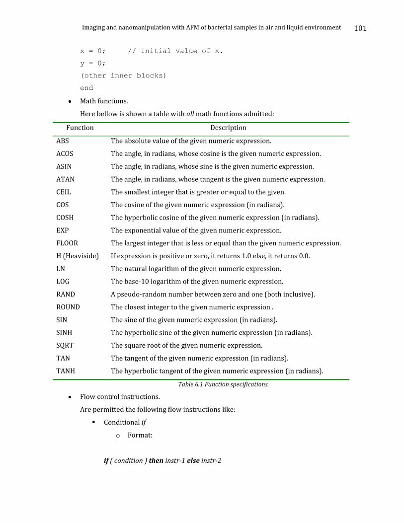
Imaging and nanomanipulation with AFM of bacterial samples in air and liquid environment
101
x = 0; // Initial value of x.
y = 0;
(other inner blocks)
end
Math functions.
Here bellow is shown a table with all math functions admitted:
Function Description
ABS The absolute value of the given numeric expression.
ACOS The angle, in radians, whose cosine is the given numeric expression.
ASIN The angle, in radians, whose sine is the given numeric expression.
ATAN The angle, in radians, whose tangent is the given numeric expression.
CEIL The smallest integer that is greater or equal to the given.
COS The cosine of the given numeric expression (in radians).
COSH The hyperbolic cosine of the given numeric expression (in radians).
EXP The exponential value of the given numeric expression.
FLOOR The largest integer that is less or equal than the given numeric expression.
H (Heaviside) If expression is positive or zero, it returns 1.0 else, it returns 0.0.
LN The natural logarithm of the given numeric expression.
LOG The base-10 logarithm of the given numeric expression.
RAND A pseudo-random number between zero and one (both inclusive).
ROUND The closest integer to the given numeric expression .
SIN The sine of the given numeric expression (in radians).
SINH The hyperbolic sine of the given numeric expression (in radians).
SQRT The square root of the given numeric expression.
TAN The tangent of the given numeric expression (in radians).
TANH The hyperbolic tangent of the given numeric expression (in radians).
Table 6.1 Function specifications.
Flow control instructions.
Are permitted the following flow instructions like:
Conditional if
o Format:
if ( condition ) then instr-1 else instr-2
Imaging and nanomanipulation with AFM of bacterial samples in air and liquid environment
102
The else part is optional.
Instr-1 will be executed if condition is true, else instr-2 will do.
Both, instr-1 and instr-2 can be instruction blocks.
for and while
o for (var = init to end step s) do inst
Var: a valid variable identifier. It cannot be assigned in the instruction inst (it can be
read, of course)
Init and end must be either numeric constants or numeric constant variables, and
end must be greater or equal than init. (if not, step s must be negative).
Inst: an instruction or block to be executed.
o While (condition) do inst
Inst: an instruction or block to be executed.
Operators.
All the basic operators can be used for simple mathematical operations. The table bellow
classifies them in three categories.
Arithmetic Relational Logical
Exponentiation (^) Less than (<) Or
Negation (-) Less than or equal to (<=) And
Product (*) Greater than (>) Xor
Division (/) Greater than or equal to (>=) Not
Modulus (%) Equality (==)
Addition subtraction (+, -) Inequality (!=)
Table 6.2 Operators used in lithography section.
Drawing instruction.
The constructors of lithography session have defined a drawing instruction as bellow: ”A
drawing instruction is an instruction that just moves the tip in the XY direction.”
So the drawing instructions available are:
1. Point, plots a point in the desired X, Y coordinates.
Point (point = (X nm, Y nm))
Where Xnm, Y nm are the absolute coordinates of the point in nanometers.
Imaging and nanomanipulation with AFM of bacterial samples in air and liquid environment
103
2. Line, draws a single line.
Line (begin = (NanometersX1, NanometersY1), end =
(NanometersX2, NanometersY2),InputChannels = (“IChn1”,
“IChn2”,…, “IChnn” ), NumPoints = NumPoints, Smooth = bool)
NanometersXi and NanometersYi are absolute coordinates of a point.
IChn1,…IChnn: list with input channel names.
NumPoints: number of points to acquire.
Smooth: whether the acquired curve must be smoothed (optional).
3. Text, draws a single line of text defined in the pattern.
Text (text = “Text”, position = (XNm, YNm), size = Size,
font = Font, stretch = Stretch)
“Text”: text to put in the view.
Size: height of the text in nanometers.
Font: name of the font used when drawing the text. If omitted, default font.
Non-drawing instructions.
Instead the non-drawing instructions are more and differ in their use and functionality, like
piezo movements, DA parameters change etc. Are defined from the constructor simply as: “A
non drawing instruction is an instruction that perform an action different from moving the tip in
the XY direction.”
o SetValue
o SetFeedback
o SetMovementSpeed
o SetPlaneScan
o Sleep
o ZMove
o DoRamp
o GetValue
o ReadDigitalBit
o ReadDigitalByte
o WriteDigitalBit
o WriteDigitalByte
o SetDynamic
o SetDrawingConfig
We aren’t going to describe all of them here but we would like to describe the most used.
o SetFeedback(Index=feedback_index,active=bool,P=Pvalue,I=Ival
ue,SetPoint=setpointvalue,InputChannel=“IChn”)
In this inststruction all arguments are optional.
active (true or false): turns feedback on/off.
Pvalue, Ivalue: feedback proportional and integral parameters.
Imaging and nanomanipulation with AFM of bacterial samples in air and liquid environment
104
setpointvalue: set point value in the feedback loop. Same
units as in acquisition frame.
InputChannel: feedback channel name.
Index is a number specifying the feedback type.
Pvalue,Ivalue: when using feedback_index_xy.
Pvalue: represents the Power feedback parameter. In such a case, the Ivalue is
ignored. When using other feedback type, these values are mutually inclusive: omit
both of them or set the two values.
SetPoint: this value is ignored when using feedback_index_xy.
o ZMove (height = nm, speed = nm/sec)
nm: height change of the tip from the current position. For negative values tip moves
away from the sample. Positive values are allowed but should be used with care.
speed: average movement speed in nm/sec (optional).
o DoRamp(InputChannels=(“IChn1”,“IChn2”,…,“IChnn”),
OutputChannel=“OChn”, NumPoints=numPoints,
InitialValue=iVal, RampAmplitude=amp, Speed=speed,
point=(XNm,YNm), SaveData=bool, Smooth=boolean,
LimitChannel=“LChn”, LimitValue=lval, RelativeLimit=bool,
OutputChannel2=“OChn2”, InitialValue2=iVal2,
RampAmplitude2=amp2)
Applies a ramp through an output channel while acquires through an Input channel.
Example: force vs distance (force→input, distance →output) or current vs voltage
(current→input, voltage →output) where:
numPoints: number of points that will be acquired (from 2 and 4096).
iVal: initial ramp value in real units of the ramp.
amp: ramp amplitude in real units. A negative value means an inversion in directions.
6.3 Automation of probe movements
While thinking over tip movement automation immediately comes in mind FZ curves. This because
while using the software given by the microscope producers is normal to make FZ curves after tip
approaches sample surface. This because can be present artefacts (see chapter 4.1.6).
Due to drift problems present in all piezoelectric actuators, normally isn’t possible to eliminate
error in positioning even when is possible to determine the correct coordinates of point. For this

Imaging and nanomanipulation with AFM of bacterial samples in air and liquid environment
105
reason that sometimes is interesting to make FZ curves in a ROI, that includes the desired point.
There are few jobs done by different groups who have practiced this technique for determining
Young’s modules
6.3.1 Making Force Vs Displacement curves in a determined point
WSxM software includes a function for making FZ curves over the sample, which is under
acquisition. There is an inconvenience; it isn’t possible to define the exact coordinates where FZ
curve is done. In this way when FZ dialog activates, the microscope makes a FZ curve in the middle
of the line where is scanning.
This is really a big limitation for two main reasons:
It’s not possible to make FZ curve in a point different from the middle one.
For making FZ curve, there is needed to wait until the desired line is under acquisition and
later activate the FZ dialog.
In the following we have defined scrip that makes FZ curves over the sample under acquisition in
the specified coordinates introduced by the AFM user in lithography section.
This is a first version of FZcurves function and the substrate used was Pseudomonas over gold.
Image 6.4 is acquired in AC mode and shows how it looks like the surface before applying the script.
We can distinguish clearly two types of substrates: pseudomonas membranes and clean gold surface
exempt form residues.
Image 6.4 Pseudomonas Au. over gold,(Left) topography (Right) 3D Reconstruction.
Imaging and nanomanipulation with AFM of bacterial samples in air and liquid environment
106
The related source code applied was(See Appendix D).In the whole begin-end block we can
distinguish three phases:
Control instructions like: Feedback switched off and dynamic switched off.
Effective movement composed from: Zmove and DoRamp.
Re-establishing previous parameters like: feedback dynamic and positioning.
Over gold substrate the F-Z curve was:
Image 6.5 (Right) FZ curve over gold substrate. (Left) Green cross showing position were FZ applied.
Over Pseudomonas au. membrane, the F-Z curve was like above. Here we note the adhesion of tip
with the membrane gives the classical V shape of the curve in the final state where the tip uncouples
from the membrane. This V shape isn’t present in the previous image were the forces of coupling
between tip and gold surface are practically inexistent.
Image 6.6 (Right) FZ curve over membrane. (Left) Green cross, positioned in the left side of the picture.
Imaging and nanomanipulation with AFM of bacterial samples in air and liquid environment
107
Meanwhile, in another situation, we could get the FZ curve of Image 6.7.Is important to note that a
possible automation could be repeatedly make FZ curves over the same substrate following some
criteria like:
FZ curves in a horizontal/vertical line.
FZ curves over a matrix (Important for making Force Volume).
Image 6.7 Other FZ curve over membrane.
6.3.2 Multiple Force Vs Displacement curves in a line and in a matrix
As remarked before, there is the possibility to automate the process of making FZ curves even in
different points. In this way are going to show a short script for making an arbitrary number of FZ
curves in a line. In image 6.8 is illustrated a series of FZ curves over a PMMA grid. While over a
matrix there is needed a nested loop like is shown:
begin
numeric x
numeric y
for (x = -500 to 500 step 100) do
begin
for (y =-500 to 500 step 100) do
Point (point = (x, y))
end
end
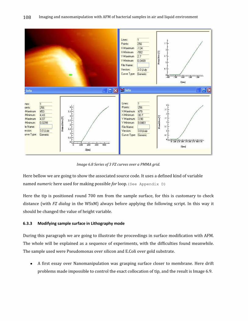
Imaging and nanomanipulation with AFM of bacterial samples in air and liquid environment
108
Image 6.8 Series of 3 FZ curves over a PMMA grid.
Here bellow we are going to show the associated source code. It uses a defined kind of variable
named numeric here used for making possible for loop.(See Appendix D)
Here the tip is positioned round 700 nm from the sample surface, for this is customary to check
distance (with FZ dialog in the WSxM) always before applying the following script. In this way it
should be changed the value of height variable.
6.3.3 Modifying sample surface in Lithography mode
During this paragraph we are going to illustrate the proceedings in surface modification with AFM.
The whole will be explained as a sequence of experiments, with the difficulties found meanwhile.
The sample used were Pseudomonas over silicon and E.Coli over gold substrate.
A first essay over Nanomanipulation was grasping surface closer to membrane. Here drift
problems made impossible to control the exact collocation of tip, and the result is Image 6.9.
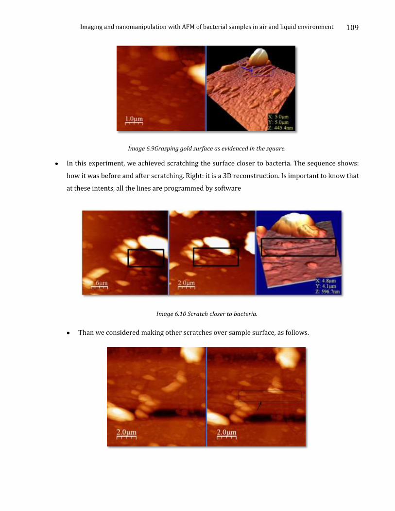
Imaging and nanomanipulation with AFM of bacterial samples in air and liquid environment
109
Image 6.9Grasping gold surface as evidenced in the square.
In this experiment, we achieved scratching the surface closer to bacteria. The sequence shows:
how it was before and after scratching. Right: it is a 3D reconstruction. Is important to know that
at these intents, all the lines are programmed by software
Image 6.10 Scratch closer to bacteria.
Than we considered making other scratches over sample surface, as follows.
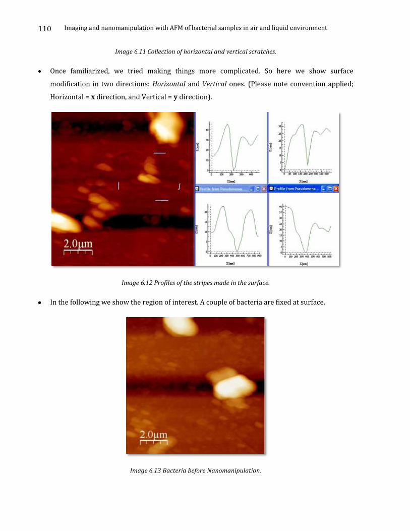
Imaging and nanomanipulation with AFM of bacterial samples in air and liquid environment
110
Image 6.11 Collection of horizontal and vertical scratches.
Once familiarized, we tried making things more complicated. So here we show surface
modification in two directions: Horizontal and Vertical ones. (Please note convention applied;
Horizontal = x direction, and Vertical = y direction).
Image 6.12 Profiles of the stripes made in the surface.
In the following we show the region of interest. A couple of bacteria are fixed at surface.
Image 6.13 Bacteria before Nanomanipulation.
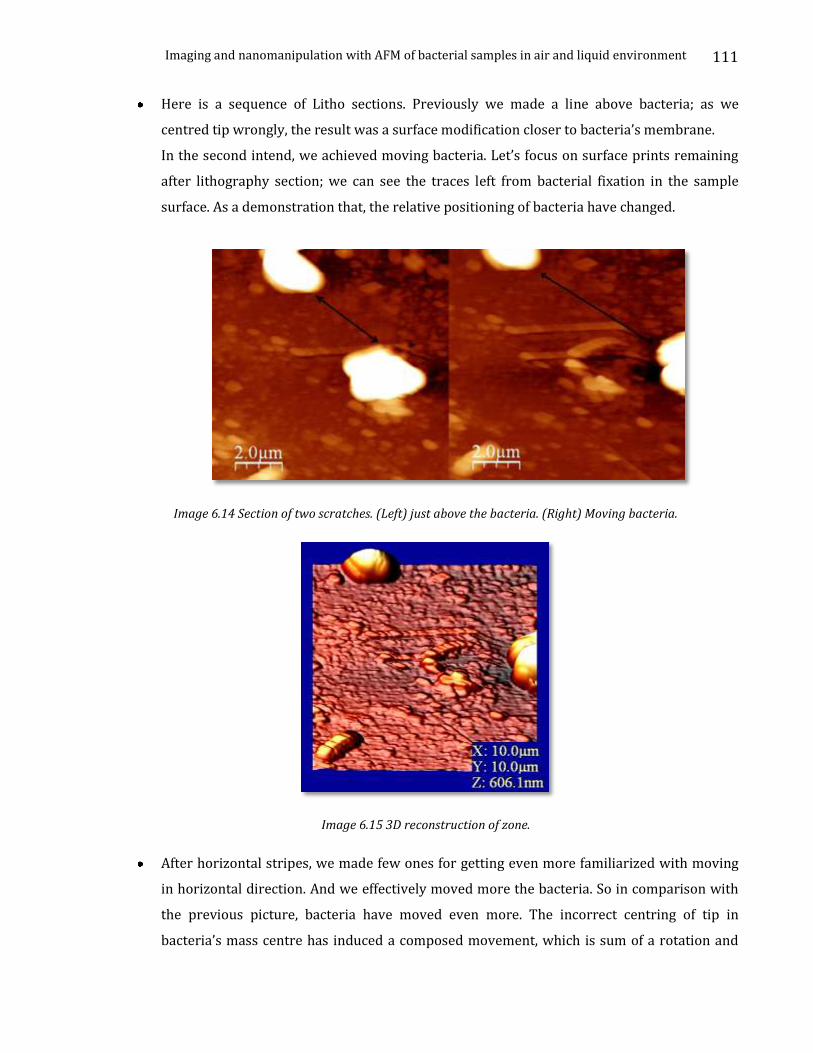
Imaging and nanomanipulation with AFM of bacterial samples in air and liquid environment
111
Here is a sequence of Litho sections. Previously we made a line above bacteria; as we
centred tip wrongly, the result was a surface modification closer to bacteria’s membrane.
In the second intend, we achieved moving bacteria. Let’s focus on surface prints remaining
after lithography section; we can see the traces left from bacterial fixation in the sample
surface. As a demonstration that, the relative positioning of bacteria have changed.
Image 6.14 Section of two scratches. (Left) just above the bacteria. (Right) Moving bacteria.
Image 6.15 3D reconstruction of zone.
After horizontal stripes, we made few ones for getting even more familiarized with moving
in horizontal direction. And we effectively moved more the bacteria. So in comparison with
the previous picture, bacteria have moved even more. The incorrect centring of tip in
bacteria’s mass centre has induced a composed movement, which is sum of a rotation and
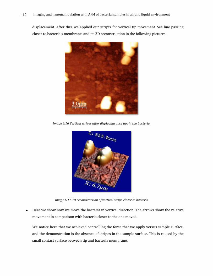
Imaging and nanomanipulation with AFM of bacterial samples in air and liquid environment
112
displacement. After this, we applied our scripts for vertical tip movement. See line passing
closer to bacteria’s membrane, and its 3D reconstruction in the following pictures.
Image 6.16 Vertical stripes after displacing once again the bacteria.
Image 6.17 3D reconstruction of vertical stripe closer to bacteria
Here we show how we move the bacteria in vertical direction. The arrows show the relative
movement in comparison with bacteria closer to the one moved.
We notice here that we achieved controlling the force that we apply versus sample surface,
and the demonstration is the absence of stripes in the sample surface. This is caused by the
small contact surface between tip and bacteria membrane.
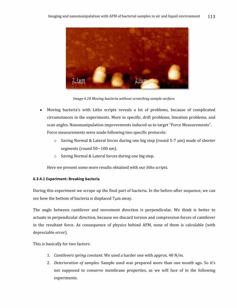
Imaging and nanomanipulation with AFM of bacterial samples in air and liquid environment
113
Image 6.18 Moving bacteria without scratching sample surface.
Moving bacteria’s with Litho scripts reveals a lot of problems, because of complicated
circumstances in the experiments. More in specific, drift problems, lineation problems, and
scan angles. Nanomanipulation improvements induced us to target “Force Measurements”.
Force measurements were made following two specific protocols:
o Saving Normal & Lateral forces during one big step (round 5-7 m) made of shorter
segments (round 50~100 nm).
o Saving Normal & Lateral forces during one big step.
Here we present some more results obtained with our litho scripts.
6.3.4.1 Experiment: Breaking bacteria
During this experiment we scrape up the final part of bacteria. In the before-after sequence, we can
see how the bottom of bacteria is displaced 7 m away.
The angle between cantilever and movement direction is perpendicular. We think is better to
actuate in perpendicular direction, because we discard torsion and compression forces of cantilever
in the resultant force. As consequence of physics behind AFM, none of them is calculable (with
depreciable error).
This is basically for two factors:
1. Cantilevers spring constant. We used a harder one with approx. 40 N/m.
2. Deterioration of samples. Sample used was prepared more than one month ago. So it’s
not supposed to conserve membrane properties, as we will face of in the following
experiments.
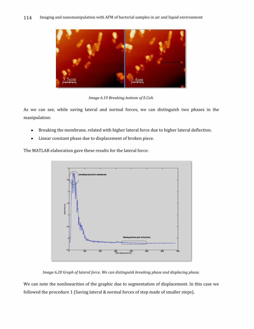
Imaging and nanomanipulation with AFM of bacterial samples in air and liquid environment
114
Image 6.19 Breaking bottom of E.Coli.
As we can see, while saving lateral and normal forces, we can distinguish two phases in the
manipulation:
Breaking the membrane, related with higher lateral force due to higher lateral deflection.
Linear constant phase due to displacement of broken piece.
The MATLAB elaboration gave these results for the lateral force:
Image 6.20 Graph of lateral force. We can distinguish breaking phase and displacing phase.
We can note the nonlinearities of the graphic due to segmentation of displacement. In this case we
followed the procedure 1 (Saving lateral & normal forces of step made of smaller steps).
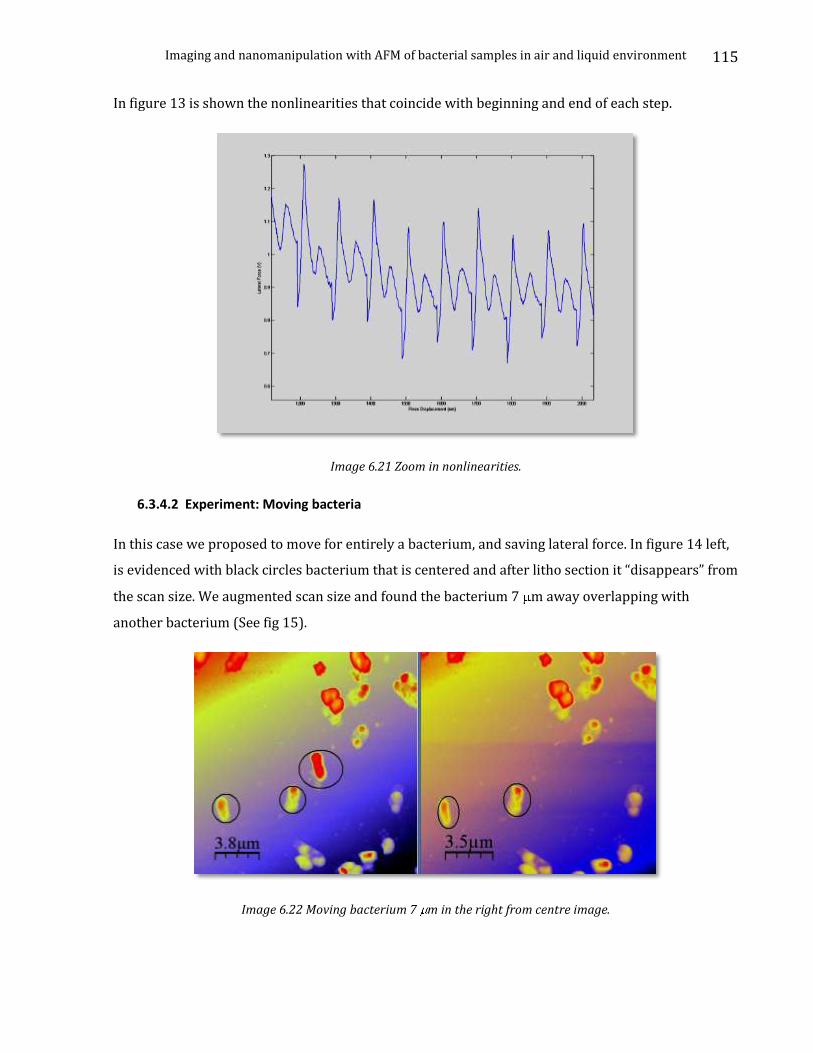
Imaging and nanomanipulation with AFM of bacterial samples in air and liquid environment
115
In figure 13 is shown the nonlinearities that coincide with beginning and end of each step.
Image 6.21 Zoom in nonlinearities.
6.3.4.2 Experiment: Moving bacteria
In this case we proposed to move for entirely a bacterium, and saving lateral force. In figure 14 left,
is evidenced with black circles bacterium that is centered and after litho section it “disappears” from
the scan size. We augmented scan size and found the bacterium 7 m away overlapping with
another bacterium (See fig 15).
Image 6.22 Moving bacterium 7 m in the right from centre image.
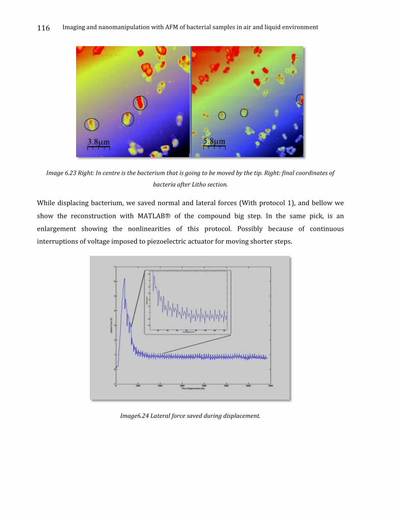
Imaging and nanomanipulation with AFM of bacterial samples in air and liquid environment
116
Image 6.23 Right: In centre is the bacterium that is going to be moved by the tip. Right: final coordinates of
bacteria after Litho section.
While displacing bacterium, we saved normal and lateral forces (With protocol 1), and bellow we
show the reconstruction with MATLAB of the compound big step. In the same pick, is an
enlargement showing the nonlinearities of this protocol. Possibly because of continuous
interruptions of voltage imposed to piezoelectric actuator for moving shorter steps.
Image6.24 Lateral force saved during displacement.
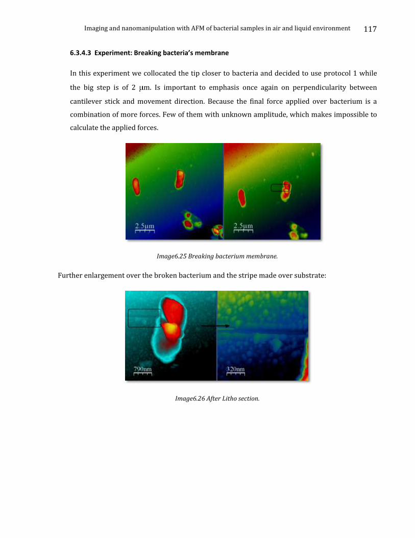
Imaging and nanomanipulation with AFM of bacterial samples in air and liquid environment
117
6.3.4.3 Experiment: Breaking bacteria’s membrane
In this experiment we collocated the tip closer to bacteria and decided to use protocol 1 while
the big step is of 2 m. Is important to emphasis once again on perpendicularity between
cantilever stick and movement direction. Because the final force applied over bacterium is a
combination of more forces. Few of them with unknown amplitude, which makes impossible to
calculate the applied forces.
Image6.25 Breaking bacterium membrane.
Further enlargement over the broken bacterium and the stripe made over substrate:
Image6.26 After Litho section.

Imaging and nanomanipulation with AFM of bacterial samples in air and liquid environment
118
Image6.27 3D reconstruction of scratch.
MATLAB post elaboration of lateral forces saved during lithography section. Is important this kind
of experiment because the pendent of the graph shows stiffness of bacterium membrane, despite
the fact that here bacteria’s are dry and deteriorated.
Image 6.28 Lateral force while breaking the membrane.
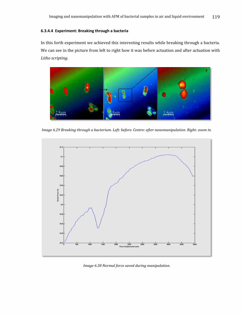
Imaging and nanomanipulation with AFM of bacterial samples in air and liquid environment
119
6.3.4.4 Experiment: Breaking through a bacteria
In this forth experiment we achieved this interesting results while breaking through a bacteria.
We can see in the picture from left to right how it was before actuation and after actuation with
Litho scripting.
Image 6.29 Breaking through a bacterium. Left: before. Centre: after nanomanipulation. Right: zoom in.
Image 6.30 Normal force saved during manipulation.
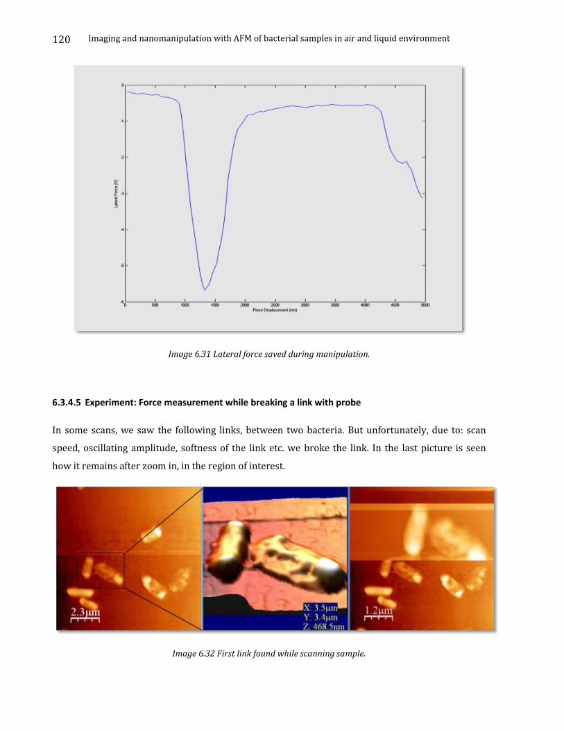
Imaging and nanomanipulation with AFM of bacterial samples in air and liquid environment
120
Image 6.31 Lateral force saved during manipulation.
6.3.4.5 Experiment: Force measurement while breaking a link with probe
In some scans, we saw the following links, between two bacteria. But unfortunately, due to: scan
speed, oscillating amplitude, softness of the link etc. we broke the link. In the last picture is seen
how it remains after zoom in, in the region of interest.
Image 6.32 First link found while scanning sample.
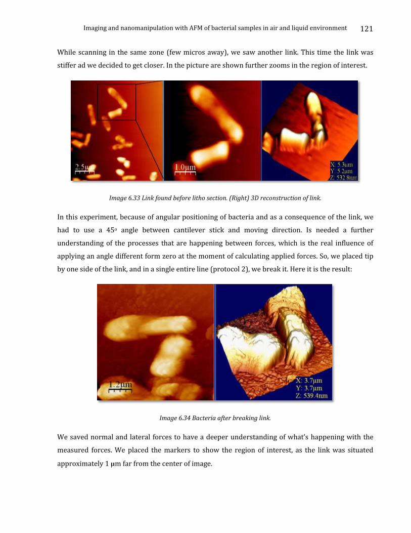
Imaging and nanomanipulation with AFM of bacterial samples in air and liquid environment
121
While scanning in the same zone (few micros away), we saw another link. This time the link was
stiffer ad we decided to get closer. In the picture are shown further zooms in the region of interest.
Image 6.33 Link found before litho section. (Right) 3D reconstruction of link.
In this experiment, because of angular positioning of bacteria and as a consequence of the link, we
had to use a 45o angle between cantilever stick and moving direction. Is needed a further
understanding of the processes that are happening between forces, which is the real influence of
applying an angle different form zero at the moment of calculating applied forces. So, we placed tip
by one side of the link, and in a single entire line (protocol 2), we break it. Here it is the result:
Image 6.34 Bacteria after breaking link.
We saved normal and lateral forces to have a deeper understanding of what’s happening with the
measured forces. We placed the markers to show the region of interest, as the link was situated
approximately 1 m far from the center of image.
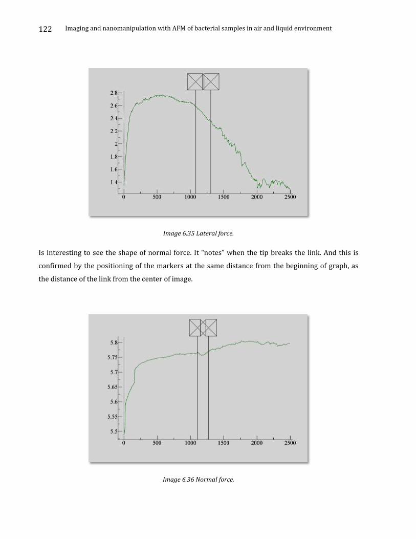
Imaging and nanomanipulation with AFM of bacterial samples in air and liquid environment
122
Image 6.35 Lateral force.
Is interesting to see the shape of normal force. It “notes” when the tip breaks the link. And this is
confirmed by the positioning of the markers at the same distance from the beginning of graph, as
the distance of the link from the center of image.
Image 6.36 Normal force.
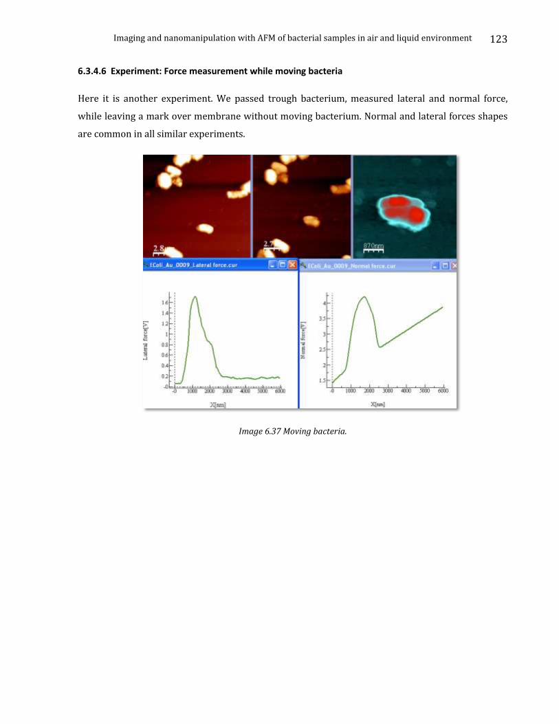
Imaging and nanomanipulation with AFM of bacterial samples in air and liquid environment
123
6.3.4.6 Experiment: Force measurement while moving bacteria
Here it is another experiment. We passed trough bacterium, measured lateral and normal force,
while leaving a mark over membrane without moving bacterium. Normal and lateral forces shapes
are common in all similar experiments.
Image 6.37 Moving bacteria.
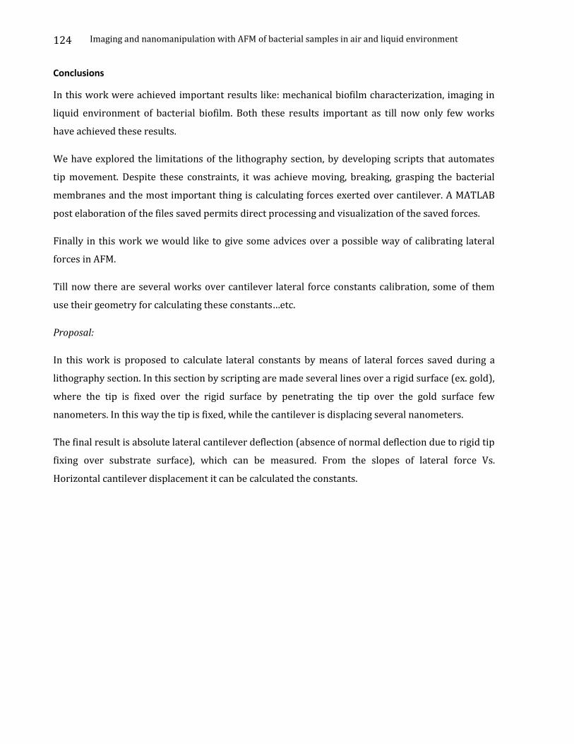
Imaging and nanomanipulation with AFM of bacterial samples in air and liquid environment
124
Conclusions
In this work were achieved important results like: mechanical biofilm characterization, imaging in
liquid environment of bacterial biofilm. Both these results important as till now only few works
have achieved these results.
We have explored the limitations of the lithography section, by developing scripts that automates
tip movement. Despite these constraints, it was achieve moving, breaking, grasping the bacterial
membranes and the most important thing is calculating forces exerted over cantilever. A MATLAB
post elaboration of the files saved permits direct processing and visualization of the saved forces.
Finally in this work we would like to give some advices over a possible way of calibrating lateral
forces in AFM.
Till now there are several works over cantilever lateral force constants calibration, some of them
use their geometry for calculating these constants…etc.
Proposal:
In this work is proposed to calculate lateral constants by means of lateral forces saved during a
lithography section. In this section by scripting are made several lines over a rigid surface (ex. gold),
where the tip is fixed over the rigid surface by penetrating the tip over the gold surface few
nanometers. In this way the tip is fixed, while the cantilever is displacing several nanometers.
The final result is absolute lateral cantilever deflection (absence of normal deflection due to rigid tip
fixing over substrate surface), which can be measured. From the slopes of lateral force Vs.
Horizontal cantilever displacement it can be calculated the constants.
Imaging and nanomanipulation with AFM of bacterial samples in air and liquid environment
125
Acknowledgments
The author of this master thesis would like to give special thanksto all of them who in a way or
another sustained and collaborated in this work:
University of Padua, for the double degree exchange program.
Dr. Antóni Juárez and Dr. Rosa Banyos, for biological sample preparation.
Dr. Manel Puig I Vidal for his supervision.
Phd.thesis student Jorge Otero Díaz for its constant help during first stages in imaging with
AFM, and with the optical microscopy.
Dr. David Lewis, from Nanonics, for the images of MultiView4000.
My family how has always supported me morally.

Imaging and nanomanipulation with AFM of bacterial samples in air and liquid environment
126
Appendix A
Gram staining (or Gram's method) is an empirical method of differentiating bacterial species into two
large groups (Gram-positive and Gram-negative) based on the chemical and physical properties of
their cell walls.A cell wall is: A fairly
rigid layer surrounding a cell, located external to the cell membrane, which provides the cell with
structural support, protection, and acts as a filtering mechanism. The cell wall also prevents over-
expansion when water enters the cell. They are found in plants, bacteria, archaea, fungi, and algae.
Animals and most protists do not have cell walls.
The material in a cell wall varies between species. In plants, the strongest component of the complex
cell wall is a carbohydratepolymer called cellulose.
The wall gives cells rigidity and strength, offering protection against mechanical stress. In
multicellular organisms, it permits the organism to build and hold its shape (morphogenesis). The
cell wall also limits the entry of large molecules that may be toxic to the cell. It further permits the
creation of a stable osmotic environment by preventing osmotic lysis and helping to retain water. In
figure A.1 is shown in left a generic cell wall, and on the right a schematic representation of it.
Appendix A.1 (Left) Cellular wall. (Right) Schematic representation of cell.
The Gram’s method is named after its inventor, the Danish scientist Hans Christian Gram (1853 –
1938), who developed the technique in 1884 to discriminate between pneumococci and Klebsiella
pneumoniae bacteria.
Uses in Research
The Gram stain is not an infallible tool for diagnosis, identification, or phylogeny, however. It is of
extremely limited use in environmental microbiology, and has been largely superseded by
molecular techniques even in the medical microbiology lab. Given that some organisms are Gram-
variable (i.e. they may stain either negative or positive), and that some organisms are not
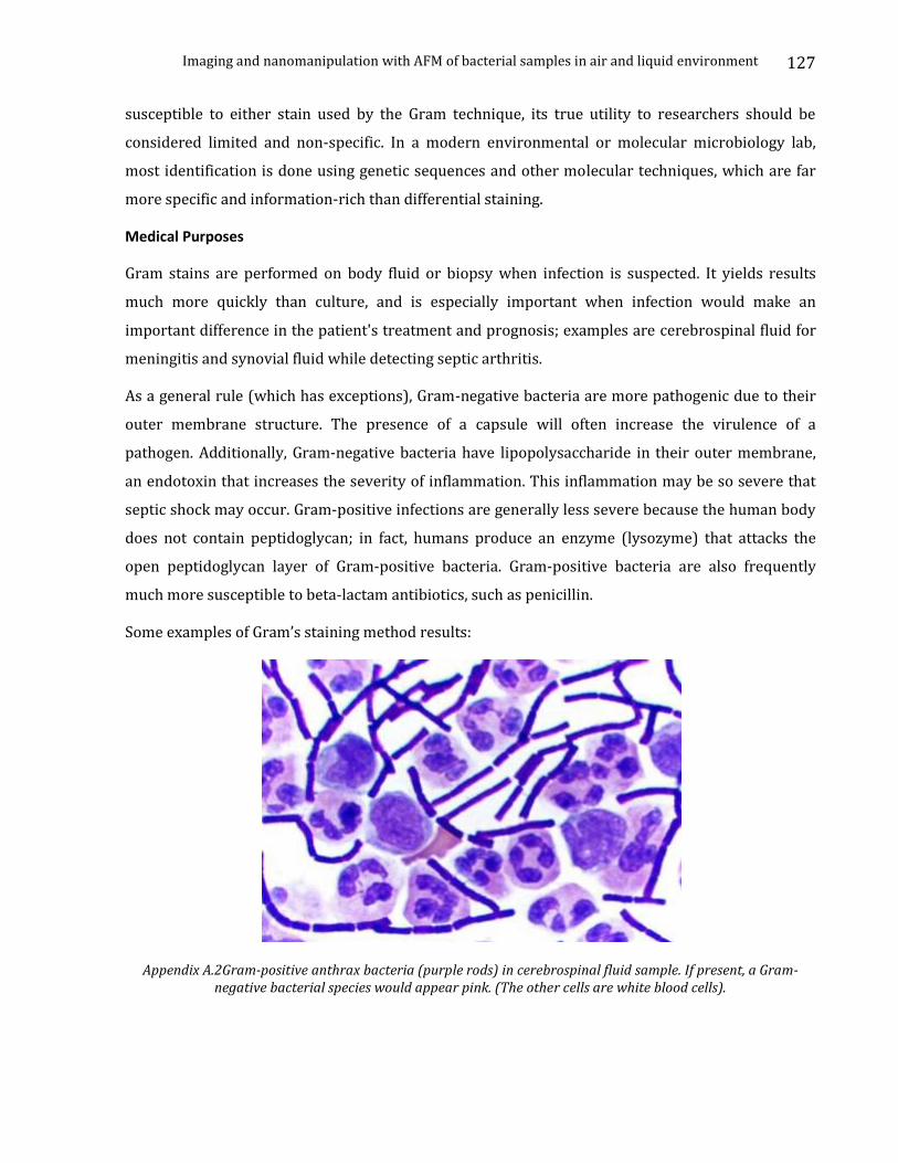
Imaging and nanomanipulation with AFM of bacterial samples in air and liquid environment
127
susceptible to either stain used by the Gram technique, its true utility to researchers should be
considered limited and non-specific. In a modern environmental or molecular microbiology lab,
most identification is done using genetic sequences and other molecular techniques, which are far
more specific and information-rich than differential staining.
Medical Purposes
Gram stains are performed on body fluid or biopsy when infection is suspected. It yields results
much more quickly than culture, and is especially important when infection would make an
important difference in the patient's treatment and prognosis; examples are cerebrospinal fluid for
meningitis and synovial fluid while detecting septic arthritis.
As a general rule (which has exceptions), Gram-negative bacteria are more pathogenic due to their
outer membrane structure. The presence of a capsule will often increase the virulence of a
pathogen. Additionally, Gram-negative bacteria have lipopolysaccharide in their outer membrane,
an endotoxin that increases the severity of inflammation. This inflammation may be so severe that
septic shock may occur. Gram-positive infections are generally less severe because the human body
does not contain peptidoglycan; in fact, humans produce an enzyme (lysozyme) that attacks the
open peptidoglycan layer of Gram-positive bacteria. Gram-positive bacteria are also frequently
much more susceptible to beta-lactam antibiotics, such as penicillin.
Some examples of Gram’s staining method results:
Appendix A.2Gram-positive anthrax bacteria (purple rods) in cerebrospinal fluid sample. If present, a Gram-negative bacterial species would appear pink. (The other cells are white blood cells).
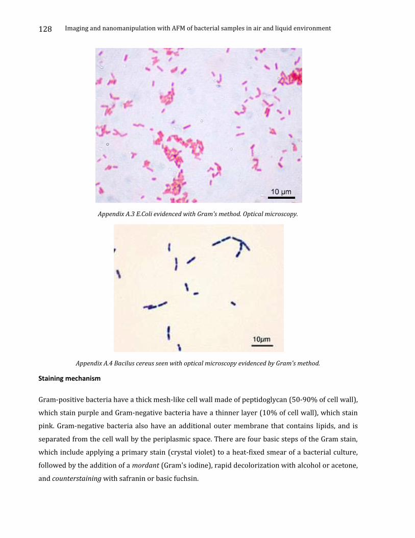
Imaging and nanomanipulation with AFM of bacterial samples in air and liquid environment
128
Appendix A.3 E.Coli evidenced with Gram's method. Optical microscopy.
Appendix A.4 Bacilus cereus seen with optical microscopy evidenced by Gram's method.
Staining mechanism
Gram-positive bacteria have a thick mesh-like cell wall made of peptidoglycan (50-90% of cell wall),
which stain purple and Gram-negative bacteria have a thinner layer (10% of cell wall), which stain
pink. Gram-negative bacteria also have an additional outer membrane that contains lipids, and is
separated from the cell wall by the periplasmic space. There are four basic steps of the Gram stain,
which include applying a primary stain (crystal violet) to a heat-fixed smear of a bacterial culture,
followed by the addition of a mordant (Gram's iodine), rapid decolorization with alcohol or acetone,
and counterstaining with safranin or basic fuchsin.
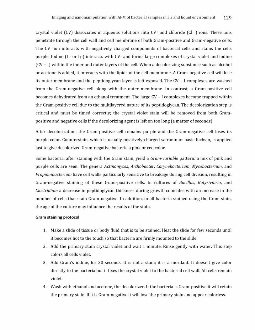
Imaging and nanomanipulation with AFM of bacterial samples in air and liquid environment
129
Crystal violet (CV) dissociates in aqueous solutions into CV+ and chloride (Cl –) ions. These ions
penetrate through the cell wall and cell membrane of both Gram-positive and Gram-negative cells.
The CV+ ion interacts with negatively charged components of bacterial cells and stains the cells
purple. Iodine (I – or I3–) interacts with CV+ and forms large complexes of crystal violet and iodine
(CV – I) within the inner and outer layers of the cell. When a decolorizing substance such as alcohol
or acetone is added, it interacts with the lipids of the cell membrane. A Gram-negative cell will lose
its outer membrane and the peptidoglycan layer is left exposed. The CV – I complexes are washed
from the Gram-negative cell along with the outer membrane. In contrast, a Gram-positive cell
becomes dehydrated from an ethanol treatment. The large CV – I complexes become trapped within
the Gram-positive cell due to the multilayered nature of its peptidoglycan. The decolorization step is
critical and must be timed correctly; the crystal violet stain will be removed from both Gram-
positive and negative cells if the decolorizing agent is left on too long (a matter of seconds).
After decolorization, the Gram-positive cell remains purple and the Gram-negative cell loses its
purple color. Counterstain, which is usually positively-charged safranin or basic fuchsin, is applied
last to give decolorized Gram-negative bacteria a pink or red color.
Some bacteria, after staining with the Gram stain, yield a Gram-variable pattern: a mix of pink and
purple cells are seen. The genera Actinomyces, Arthobacter, Corynebacterium, Mycobacterium, and
Propionibacterium have cell walls particularly sensitive to breakage during cell division, resulting in
Gram-negative staining of these Gram-positive cells. In cultures of Bacillus, Butyrivibrio, and
Clostridium a decrease in peptidoglycan thickness during growth coincides with an increase in the
number of cells that stain Gram-negative. In addition, in all bacteria stained using the Gram stain,
the age of the culture may influence the results of the stain.
Gram staining protocol
1. Make a slide of tissue or body fluid that is to be stained. Heat the slide for few seconds until
it becomes hot to the touch so that bacteria are firmly mounted to the slide.
2. Add the primary stain crystal violet and wait 1 minute. Rinse gently with water. This step
colors all cells violet.
3. Add Gram's iodine, for 30 seconds. It is not a stain; it is a mordant. It doesn't give color
directly to the bacteria but it fixes the crystal violet to the bacterial cell wall. All cells remain
violet.
4. Wash with ethanol and acetone, the decolorizer. If the bacteria is Gram-positive it will retain
the primary stain. If it is Gram-negative it will lose the primary stain and appear colorless.
Imaging and nanomanipulation with AFM of bacterial samples in air and liquid environment
130
Appendix B
Manual of Lithography
This support note shows how to use lithography section of WSxM program. It will describe each one of
the menus that appear in the subprogram.
Lithography is a part of the WSxM program. In this frame you can draw on a sample, define the tip
motion and write on a sample.
Introduction
WSxM Lithography section allows you to move the tip over the sample performing different actions.
You can think in the tip as a pen, and the sample as a paper. If you can somehow define what does
“draw” mean, you can “draw” with your tip over your sample, (like) as it was a pen. When you have
a pen, you can move it far away from the paper and it will draw nothing. The same can be done with
WSxM Lithography if you can define what “do not draw” means in your tip-sample system.
When you plot a simple figure, like a line or a set of concatenated lines, the tip will go to the desired
starting point. Once reached that point, if you have defined what “draw” means in your system,
these actions will be performed. This is what we have called “Start drawing actions”(we will see this
feature in more detail in a few lines). In our pen-paper example, this is like moving the pen to the
paper until they contact. Then, the tip will move following a path, drawing. When the figure is
complete, the system will perform “Finish drawing actions”. In the pen-paper example the pen goes
out from the paper. Now the tip will move to the first point of the next figure, without drawing.
Drawing a new lithography pattern
There are two ways to input a lithography pattern:
1. Graphically. This is the easiest way and the one that we recommend.
1. 1. First of all, if the design Window is not open, you have to open it by pressing the Design
command in the View menu or its associated button in the toolbar.
1. 2. In the settings dialog-bar you can change the size of the drawing area. This dialog contains
some figure editing and simulating information, such as the size of the drawing area, the speed
of the movements during the simulation process and a check-box that allows showing or hiding
the position of the tip.
Imaging and nanomanipulation with AFM of bacterial samples in air and liquid environment
131
1.3. Now you can plot figures by pressing the Plot menu or the appropriate toolbar command.
2. Editing the associated code.
2. 1. You can see the code associated to the designed pattern by opening the code Window. You
can add lines by typing new code, changing the existing, coping and pasting the existing and so
on.
2. 2. To make effective the changes made in the code window, you may press the Apply button (a
check mark) or select this command in the Code menu.
2. 3. If you do not see the effect of the changes you did, you can verify the compilation results
window. This window will tell you if there is any syntactic error in your code. You can open it by
pressing the toolbar button or the command in the View menu.
You can select a background image for your lithography pattern. When you open an image from
the lithography main frame, this image will be placed in the background of the design window
and the size in the settings will change. If you want to auto-fit the pattern to the image, you have
to check this option in the browser settings. When you go to the new lithography main frame
from the acquisition main frame, the image in the selected channel will be placed in the
background.
You can save your session or open a saved one with the image browser, but always in the
lithography main frame.
If you are editing some code and it has syntactic errors but you want to save it, you can do this
by pressing Save Code or the button in the toolbar of the code window. If you save it by pressing
Save, it will save the pattern in the design window.
Simulating the lithography session
After you have finished drawing your lithography pattern you can simulate it. The movement
speed of the tip will be the one in the settings dialog. You can execute the whole session, only a
single block (i.e. a multiline) or a single simple instruction (i.e. single line in a multilane). The
real tip position will not vary while simulating, but there will be a simulated tip position.
Doing a real lithography session
There is a dialog-bar in the data acquisition main frame. If you open it, you will see a button to
activate/deactivatethe lithography session (in green if it is active and in gray if it is not) and
some buttons to select the execution mode, described bellow.
If there is a lithography pattern in the main lithography frame and your scan size Is different
from 0, you can activate the lithography session in the acquisition main frame. To do this, press
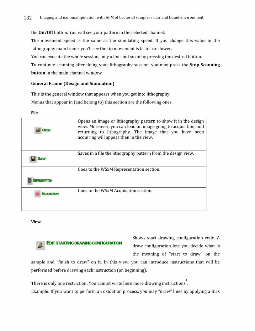
Imaging and nanomanipulation with AFM of bacterial samples in air and liquid environment
132
the On/Off button. You will see your pattern in the selected channel.
The movement speed is the same as the simulating speed. If you change this value in the
Lithography main frame, you'll see the tip movement is faster or slower.
You can execute the whole session, only a line and so on by pressing the desired button.
To continue scanning after doing your lithography session, you may press the Stop Scanning
button in the main channel window.
General Frame (Design and Simulation)
This is the general window that appears when you get into lithography.
Menus that appear in (and belong to) this section are the following ones.
File
Opens an image or lithography pattern to show it in the design view. Moreover, you can load an image going to acquisition, and returning to lithography. The image that you have been acquiring will appear then in the view.
Saves in a file the lithography pattern from the design view.
Goes to the WSxM Representation section.
Goes to the WSxM Acquisition section.
View
Shows start drawing configuration code. A
draw configuration lets you decide what is
the meaning of “start to draw” on the
sample and “finish to draw” on it. In this view, you can introduce instructions that will be
performed before drawing each instruction (on beginning).
There is only one restriction: You cannot write here more drawing instructions1.
Example: If you want to perform an oxidation process, you may “draw” lines by applying a Bias
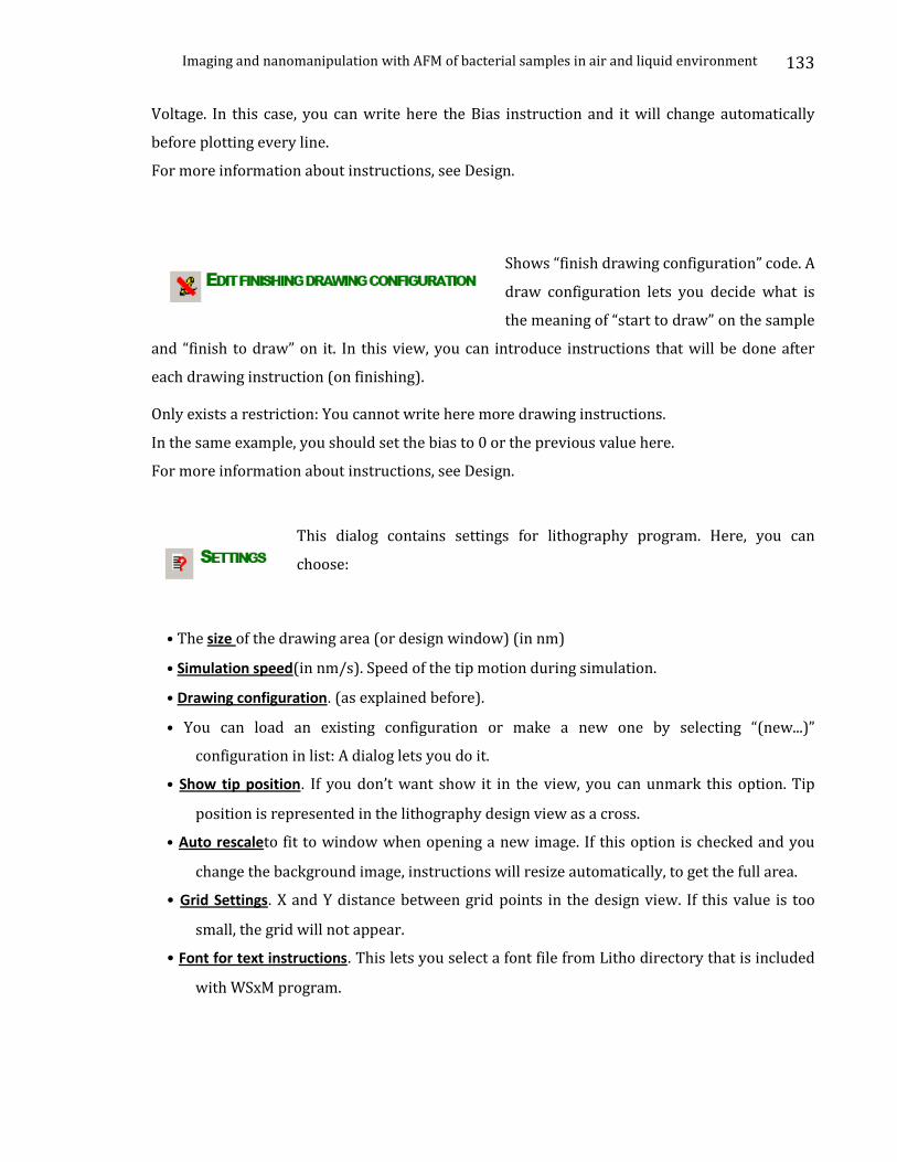
Imaging and nanomanipulation with AFM of bacterial samples in air and liquid environment
133
Voltage. In this case, you can write here the Bias instruction and it will change automatically
before plotting every line.
For more information about instructions, see Design.
Shows “finish drawing configuration” code. A
draw configuration lets you decide what is
the meaning of “start to draw” on the sample
and “finish to draw” on it. In this view, you can introduce instructions that will be done after
each drawing instruction (on finishing).
Only exists a restriction: You cannot write here more drawing instructions.
In the same example, you should set the bias to 0 or the previous value here.
For more information about instructions, see Design.
This dialog contains settings for lithography program. Here, you can
choose:
• The size of the drawing area (or design window) (in nm)
• Simulation speed(in nm/s). Speed of the tip motion during simulation.
• Drawing configuration. (as explained before).
• You can load an existing configuration or make a new one by selecting “(new...)”
configuration in list: A dialog lets you do it.
• Show tip position. If you don’t want show it in the view, you can unmark this option. Tip
position is represented in the lithography design view as a cross.
• Auto rescaleto fit to window when opening a new image. If this option is checked and you
change the background image, instructions will resize automatically, to get the full area.
• Grid Settings. X and Y distance between grid points in the design view. If this value is too
small, the grid will not appear.
• Font for text instructions. This lets you select a font file from Litho directory that is included
with WSxM program.
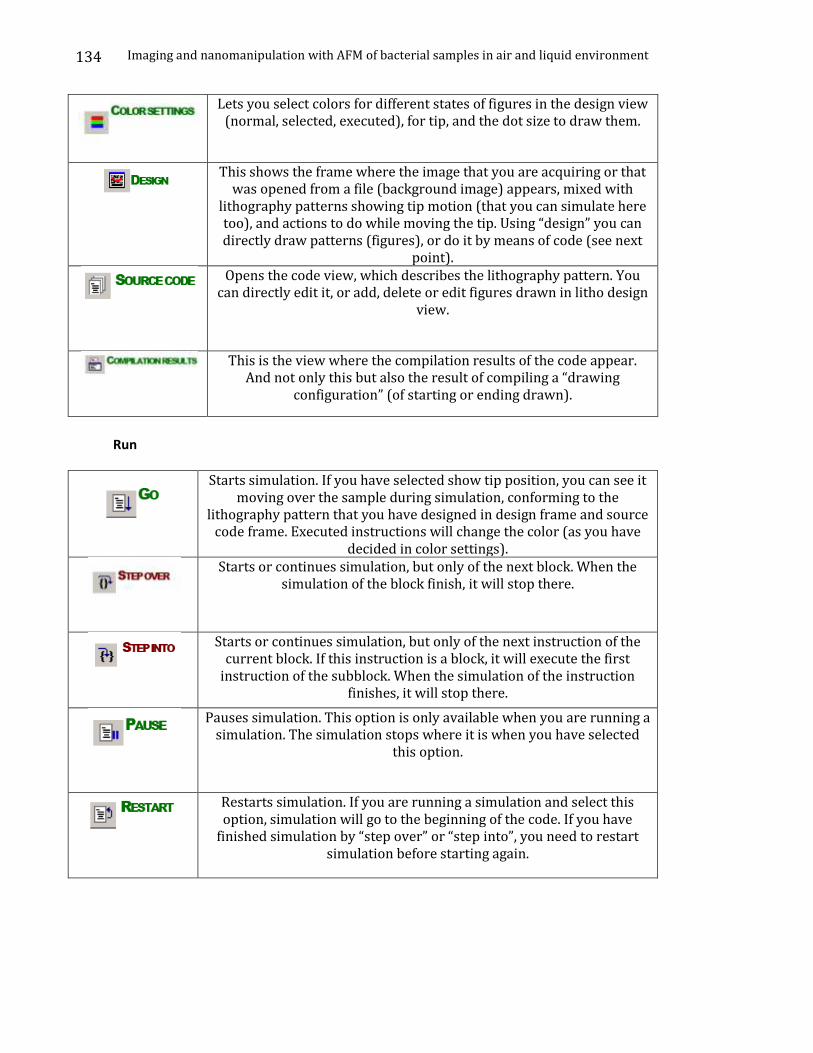
Imaging and nanomanipulation with AFM of bacterial samples in air and liquid environment
134
Lets you select colors for different states of figures in the design view (normal, selected, executed), for tip, and the dot size to draw them.
This shows the frame where the image that you are acquiring or that was opened from a file (background image) appears, mixed with
lithography patterns showing tip motion (that you can simulate here too), and actions to do while moving the tip. Using “design” you can directly draw patterns (figures), or do it by means of code (see next
point).
Opens the code view, which describes the lithography pattern. You can directly edit it, or add, delete or edit figures drawn in litho design
view.
This is the view where the compilation results of the code appear.
And not only this but also the result of compiling a “drawing configuration” (of starting or ending drawn).
Run
Starts simulation. If you have selected show tip position, you can see it moving over the sample during simulation, conforming to the
lithography pattern that you have designed in design frame and source code frame. Executed instructions will change the color (as you have
decided in color settings).
Starts or continues simulation, but only of the next block. When the simulation of the block finish, it will stop there.
Starts or continues simulation, but only of the next instruction of the current block. If this instruction is a block, it will execute the first
instruction of the subblock. When the simulation of the instruction finishes, it will stop there.
Pauses simulation. This option is only available when you are running a simulation. The simulation stops where it is when you have selected
this option.
Restarts simulation. If you are running a simulation and select this option, simulation will go to the beginning of the code. If you have
finished simulation by “step over” or “step into”, you need to restart simulation before starting again.
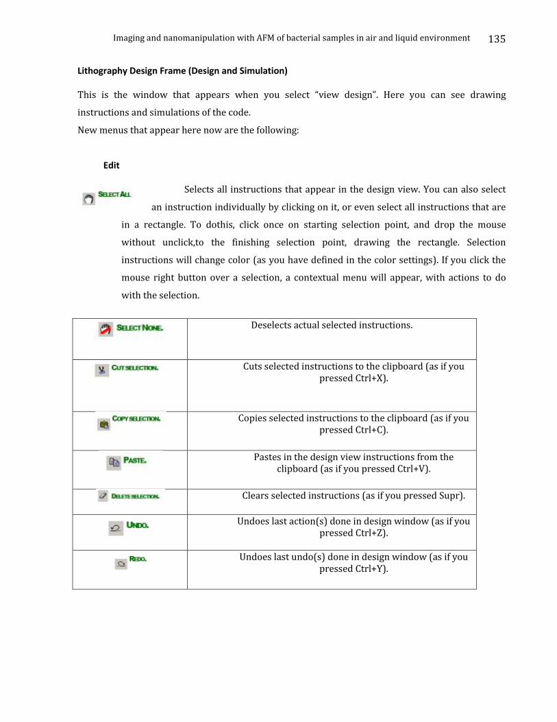
Imaging and nanomanipulation with AFM of bacterial samples in air and liquid environment
135
Lithography Design Frame (Design and Simulation)
This is the window that appears when you select “view design”. Here you can see drawing
instructions and simulations of the code.
New menus that appear here now are the following:
Edit Selects all instructions that appear in the design view. You can also select
an instruction individually by clicking on it, or even select all instructions that are
in a rectangle. To dothis, click once on starting selection point, and drop the mouse
without unclick,to the finishing selection point, drawing the rectangle. Selection
instructions will change color (as you have defined in the color settings). If you click the
mouse right button over a selection, a contextual menu will appear, with actions to do
with the selection.
Deselects actual selected instructions.
Cuts selected instructions to the clipboard (as if you pressed Ctrl+X).
Copies selected instructions to the clipboard (as if you pressed Ctrl+C).
Pastes in the design view instructions from the clipboard (as if you pressed Ctrl+V).
Clears selected instructions (as if you pressed Supr).
Undoes last action(s) done in design window (as if you pressed Ctrl+Z).
Undoes last undo(s) done in design window (as if you pressed Ctrl+Y).

Imaging and nanomanipulation with AFM of bacterial samples in air and liquid environment
136
Plot
Draws a dot in the design view. When you select it, you can click on a point of the view to select the position of the dot.
Draws a line in the design view. When you select it, you can click on a point of the view to select the start position of the line, and click again
to select the end position.
Draws a multiline in the design view. When you select it, you can click on a point of the view to select the start position of the multiline, and
click again to select the end position of each partial line.
This option shows a dialog to write a text in the design window. You can decide the height of text. After you select OK on this dialog, the
position of the text has to be defined by clicking at the corresponding location in the design view. Font can be selected in lithography
settings frame.
Source Code Frame (Design and Simulation)
Here, you can see the instructions represented in the design view, and add new instructions or
modify the existing ones. The language is not case sensitive, that is, you can type LINE or line and it
will threat both words as if they were the same one.
Instructions available are the following ones:
Assignment Instruction
Description
Assigns a value to a variable. Format
variable-ident = math-expression ;
Block
Description
Let you organize code, and simulates it as you want, using step over and step into options.
Format

Imaging and nanomanipulation with AFM of bacterial samples in air and liquid environment
137
begin
(....)
end
• Where (...) are more blocks or other instructions (without any limit).
DoRamp Instruction
Description
Acquires from the specified input channel while applying a ramp in the specified output
channel. Optionally, it can apply ramps in two different output channels simultaneously.
Format
DoRamp(InputChannels = (“IChnList”),
OutputChannel = “OChn”,
NumPoints = numPoints,
InitialValue = Unit,
RampAmplitude = Unit,
Speed = UnitPerSecond,
Point = (NanometersX, NanometersY),
SaveData = bool,
Smooth = bool,
LimitChannel = “LChn”,
LimitValue = Unit,
RelativeLimit = bool,
OutputChannel2 = “OChn2”,
InitialValue2 = Unit,
RampAmplitude2 = Unit)
• IChnList: list with input channel names.
• OChn: output channel name.
• NumPoints: number of points to acquire. It must be between 0 and 4096.
• InitialValue: initial value for acquiring the curve (optional).
• RampAmplitude: ramp amplitude.
• Speed: acquisition speed.
• NanometersX, NanometersY: coordinates where ramp will be applied.
• SaveData: whether or not the curve must be saved.
Imaging and nanomanipulation with AFM of bacterial samples in air and liquid environment
138
• Smooth: whether or not the acquired curve must be smoother.
• LChannel: limit channel name.
• LimitValue: limit value (in LimitChannel unit)
• RelativeLimit: whether or not the LimitValue is a relative limit
• OChn2: second output channel (optional).
• InitialValue2: initial value for the second output channel
• RampAmplitude2: ramp amplitude for the second output channel
Remarks
• The Unit for InitialValue, RampAmplitude and Speed is the one selected as default
unit for the specified output channel in the Output Channels Manager. The Unit
for InitialValue, RampAmplitude also applies for the second output channel, if
specified. Speed is only referred to the main output channel.
• IChnList must go between parentheses.
• Channel names must be written between quotes.
• If either OChn2 or InitialValue2 or RampAmplitude2 is specified, OChn2 and
RampAmplitude2 are then required. If limit channel and limit value are specified,
ramp acquisition will stop when the value measured in limit channel is greater
than the limit value. This limit can be either relative or absolute. These values are
mutually inclusive: you must either omit both or set the two values.
For Instruction
Description
Repeats an instruction a specified number of times.
Format
for (var = init to end step s) do instruction
Imaging and nanomanipulation with AFM of bacterial samples in air and liquid environment
139
• Var must be a valid variable identifier.
• Both, ‘init’ and ‘end’ must be either numeric constants or numeric constant
variables, and ‘end’ must be greater or equal than ‘init’
• Instruction can be a block.
• Var cannot be assigned in instruction (it can be read, of course).
• Step is optional. If not present, its value is either 1 or -1, depending on the
loop limits).
GetValue Instruction
Description
Reads a value from a channel. This instruction can be used as a numeric value (as a part of any other
instruction).
Format
GetValue (InputChannel = “IChn”, SaveData = bool)
• IChn: input channel name.
• SaveData: whether or not the value must be saved (optional). The value in
“Saving Options” will be used if omitted.
If Instruction
Description
Executes an instruction only if a certain condition evaluates to true.
Format
if ( condition ) then instr-1 [else instr-2]
• The ‘else’ part is optional.
• Both, instr-1 and instr-2 can be instruction blocks.
Line Instruction
Description
Draws a single line. This is a drawing instruction.
Format
Imaging and nanomanipulation with AFM of bacterial samples in air and liquid environment
140
Line (begin = (NanometersX1, NanometersY1),
end = (NanometersX2, NanometersY2) , InputChannels = (“IChnList”),
NumPoints = NumPoints,
Smooth = bool).
• NanometersXi and NanometersYi are absolute coordinates of a point.
• IChn: list with input channel names.
• NumPoints: number of points to acquire. It must be between 2 and 4096.
• Smooth: whether or not the acquired curve must be smoothed (optional). This argument is
false by default.
Remarks
• Begin argument is optional. If it is not specified, the beginning of the line will be the actual
tip position (it can be the finishing point of the previous line).
• IChnList, NumPoints and Smooth are optional.
Point Instruction
Description
Plots a point. This is a drawing instruction.
Format
Point (point = (NanometersX, NanometersY))
• NanometersX and NanometersY are absolute coordinates of a point.
ReadDigitalBit Instruction
Description
Reads a single bit from the user input digital signals port. This instruction can be used as a
numeric value (as a part of any other instruction).
Format
ReadDigitalBit (BitIndex = idx).
• idx is the bit index, from 0 to 7 (7 is the most significant bit)
• This instruction is only available to Dulcinea Electronics users.
ReadDigitalByte Instruction
Description
Imaging and nanomanipulation with AFM of bacterial samples in air and liquid environment
141
Reads the byte in the user input digital signals port. This instruction can be used as a numeric value
(as a part of any other instruction).
Format
ReadDigitalByte ()
• This instruction is only available to Dulcinea Electronics users.
SetDrawingConfig Instruction
Description
Changes the current drawing configuration
Format
SetDrawingConfig (Name = “ConfigName”).
• ConfigName is the configuration name. It must be written between quotes.
SetDynamic Instruction
Description
Activates or deactivates the oscillation on the dynamic card and changes the PLL state.
Format
SetDynamic (Oscillation = Bool, SwitchRelay = Bool, PLLActive = Bool,
Index = BoardIndex)
• Oscillation is stopped or restarted depending on the value of parameter Oscillation (false /
true), if present.
• When PLLActive parameter is present, it activates / deactivates the PLL on the specified
dynamic board.
• When SwitchRelay is true, the oscillation is started / stopped by changing the
corresponding bit in the digital channel. When it is false, it just resets / restores the
amplitude channel value. Default value for this parameter is false.
• BoardIndex determines over which dynamic board the changes are made. It can be either 1
(for the first dynamic board) or 2 (for the second dynamic board). Its default value is 1.
SetFeedBack Instruction
Imaging and nanomanipulation with AFM of bacterial samples in air and liquid environment
142
Description
Activates or deactivates feedback loop and set feedback parameters.
Format
SetFeedback (Index = feedback_index,
active = Bool, P = PValue, I = IValue,
setPoint = SetPointValue, InputChannel = iChn)
• All arguments are optional.
• Active (true or false) determines feedback to be turned on/off.
• PValue is the feedback proportional parameter (P).
• IValue is the feedback integral parameter (I).
• SetPointValue is value of the set point in the feedback loop. Units are the
same as you have decided in the corresponding panel of the WSxM
acquisition frame.
• InputChannel is the feedback channel.
• Index is a number specifying the feedback type. You can choose among the
following constant values:
feedback_index_main (1)
feedback_index_2nd (2)
feedback_index_3rd (3)
feedback_index_4th (4)
feedback_index_xy (10)
feedback_index_z (11)
You can use either the number or the constant.
• The meaning and need of some arguments may vary depending on the
feedback chosen:
• PValue,IValue: when using either feedback_index_xy or feedback_index_z, •
PValue represents the Power feedback parameter. In such a case, the IValue
is ignored.
When using other feedback type, these values are mutually inclusive: you
must either omit both or set the two values.
• SetPoint: this value is ignored when using either feedback_index_xy or
feedback_index_z.
Imaging and nanomanipulation with AFM of bacterial samples in air and liquid environment
143
• InputChannel: this argument is ignored when using feedback_index_xy.
SetMovementSpeed Instruction
Description
Sets the tip motion speed.
Format
SetMovementSpeed (horizontal = nm/sec, vertical = nm/sec);
• Units are in nm/sec.
• Both arguments are optional.
SetPlaneScan Instruction
Description
Activates or deactivates the planescan.
Format
SetPlaneScan(active = Bool);
SetValue Instruction
Description
Sets a value in a channel, as discussed below.
Format
SetValue (Bias = BValue); or
SetValue (OutputChannel = “OChn”, Value = OValue);
• OChn: output channel name, between quotes. Don’t use the following
channels: “X scan”, “Y scan”, “Z”.
• OValue: value to set in the specified output channel, in channel default unit.
• BValue: voltage to set in the bias output. Value must be specified in
millivolts.
Sleep Instruction
Imaging and nanomanipulation with AFM of bacterial samples in air and liquid environment
144
Description
Waits for a specified time in milliseconds.
Format
Sleep (milliseconds = msec);
• msec is time to wait.
Text Instruction
Description
Draws a single line of text. This is a drawing instruction.
Format
Text (text = “Text”, position = (NanometersX, NanometersY), size =
Size, font = Font, stretch = Stretch));
• Text is the text to put in the view.
• NanometersX and NanometersY are coordinates of the position.
• Size, is the height of the text in nanometers.
• Font is the name of the font used when drawing the text. If omitted, default.
• Stretch, is the stretching factor (optional) Its default value is 1.
Variable declaration
Description
Declares a variable with the name ‘ident’.
Format
Float identifier;
Integer identifier;
Boolean identifier;
• This will declare a new variable, of the specified type.
• Variables must be declared before using them.
• You can declare variables only in the main block and before any other
instruction.
• Float variables can hold rational numbers. You can use “Numeric”
instead of “Float” to declare this kind of variables.
Imaging and nanomanipulation with AFM of bacterial samples in air and liquid environment
145
• Integer variables can hold integers in the range -2147483648 to
2147483647.
• Boolean variables can hold the logical values true and false.
• Optionally, you can declare a const variable, by writing the const.
keyword before its name. In such case, you must provide its constant
value as in an assignment expression.
While instruction
Description
Repeats an instruction until the specified condition is false.
Format
While (condition) do instr
• Instr can be a block.
WriteDigitalBit Instruction
Description
Writes a single bit to the user output digital signals port.
Format
WriteDigitalBit (BitIndex = idx, Value = val);
• idx is the bit index, from 0 to 7 (7 is the most significant bit).
• val can be either 0 or 1.
WriteDigitalByte Instruction
Description
Writes a byte to the user output digital signals port.
Format
WriteDigitalByte (Value = val);
• val must be in the range 0 .. 255.
ZMove Instruction
Imaging and nanomanipulation with AFM of bacterial samples in air and liquid environment
146
Description
Moves tip to a given height.
Format
Zmove (height = Nanometers, speed = nm/sec);
• Nanometers is height to move the tip. Positive value goes away from the
sample, that is tip-sample distance is increased. Negative values are allowed
but should be used with care.
• nm/sec is average movement speed (optional) .
Commands available for this frame are:
Opens a code from a file, and puts it in the lithography code frame, but without loading. You can also load a Bitmap File (*.BMP). In this case, you will be asked to select the distance between the points of the bitmap (in nanometers). A new Lithography pattern made of Point instructions will be created. There will be points only in the dark zones of the bitmap.
Saves code from the frame in the actual file as is, without checking it. If code is totally new, and you have not loaded it from a file, this option will ask you for a file name.
Saves code from the frame in a new file, without checking it.
Applies code changes to the design view. Instructions are compiled, and results appear in the lithography compilation results view. If it was successful, new code will be represented in the lithography design view, and it can be simulated. During simulation the next line ready to execute will change colour. If there are errors, instruction won’t appear in the view. Warnings only indicate that something can be wrong, in spite of code compile and will be shown in the view.
Lithography Dialog – Bar
Activates/deactivates the lithography session. Activation will stop the scan (as if pressed in the selected channel acquisition window) shows the lithography pattern over the acquired image.
Appendix C
Pseudomonas aeruginosa
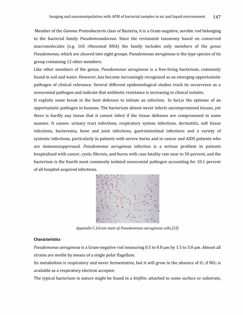
Imaging and nanomanipulation with AFM of bacterial samples in air and liquid environment
147
Member of the Gamma Proteobacteria class of Bacteria, it is a Gram-negative, aerobic rod belonging
to the bacterial family Pseudomonadaceae. Since the revisionist taxonomy based on conserved
macromolecules (e.g. 16S ribosomal RNA) the family includes only members of the genus
Pseudomonas, which are cleaved into eight groups. Pseudomonas aeruginosa is the type species of its
group containing 12 other members.
Like other members of the genus, Pseudomonas aeruginosa is a free-living bacterium, commonly
found in soil and water. However, has become increasingly recognized as an emerging opportunistic
pathogen of clinical relevance. Several different epidemiological studies track its occurrence as a
nosocomial pathogen and indicate that antibiotic resistance is increasing in clinical isolates.
It exploits some break in the host defenses to initiate an infection. In fact,is the epitome of an
opportunistic pathogen in humans. The bacterium almost never infects uncompromised tissues, yet
there is hardly any tissue that it cannot infect if the tissue defenses are compromised in some
manner. It causes: urinary tract infections, respiratory system infections, dermatitis, soft tissue
infections, bacteremia, bone and joint infections, gastrointestinal infections and a variety of
systemic infections, particularly in patients with severe burns and in cancer and AIDS patients who
are immunosuppressed. Pseudomonas aeruginosa infection is a serious problem in patients
hospitalized with cancer, cystic fibrosis, and burns with case fatality rate near to 50 percent, and the
bacterium is the fourth most commonly isolated nosocomial pathogen accounting for 10.1 percent
of all hospital-acquired infections.
Appendix C.1Gram stain of Pseudomonas aeruginosa cells.[53]
Characteristics
Pseudomonas aeruginosa is a Gram-negative rod measuring 0.5 to 0.8 µm by 1.5 to 3.0 µm. Almost all
strains are motile by means of a single polar flagellum.
Its metabolism is respiratory and never fermentative, but it will grow in the absence of O2 if NO3 is
available as a respiratory electron acceptor.
The typical bacterium in nature might be found in a biofilm, attached to some surface or substrate,

Imaging and nanomanipulation with AFM of bacterial samples in air and liquid environment
148
or in a planktonic form, as a unicellular organism, actively swimming by means of its flagellum, is
considered one of the most vigorous, fast-swimming bacteria seen in hay infusions and pond water
samples.
In its natural habitat is not particularly distinctive as a pseudomonad, but it does have a
combination of physiological traits that are noteworthy and may relate to its pathogenesis. Some
properties:
• Has very simple nutritional requirements and it is often observed "growing in distilled water",
which is evidence of its minimal nutritional needs. In the laboratory, the simplest medium for
growth consists of acetate as a source of carbon and ammonium sulfate as a source of nitrogen.
• Possesses the metabolic versatility for which pseudomonads are so renowned. Organic growth
factors are not required, and it can use more than seventy-five organic compounds for growth.
• Optimum temperature for growth is 37 degrees, and it is able to grow at temperatures as high as
42 degrees.
• Is tolerant to a wide variety of physical conditions, including temperature variations. It is resistant
to high concentrations of salts and dyes, weak antiseptics, and many commonly used antibiotics.
• Predilection for growth in moist environments, which is probably a reflection of its natural
existence in soil and water.
These natural properties of the bacterium undoubtedly contribute to its ecological success as an
opportunistic pathogen. They also help explain the ubiquitous nature of the organism and its
prominence as a nosocomial pathogen.
May produce three colony types. Natural isolates from soil or water typically produce a small, rough
colony. Clinical samples, in general, yield one or another of two smooth colony types. One type has a
fried-egg appearance, which is large, smooth, with flat edges, and an elevated appearance. Another
type, frequently obtained from respiratory and urinary tract secretions, has a mucoid appearance,
which is attributed to the production of alginate slime. The smooth and mucoid colonies are
presumed to play a role in colonization and virulence.
Appendix C.2Pseudomonas aeruginosa colonies on agar[54]
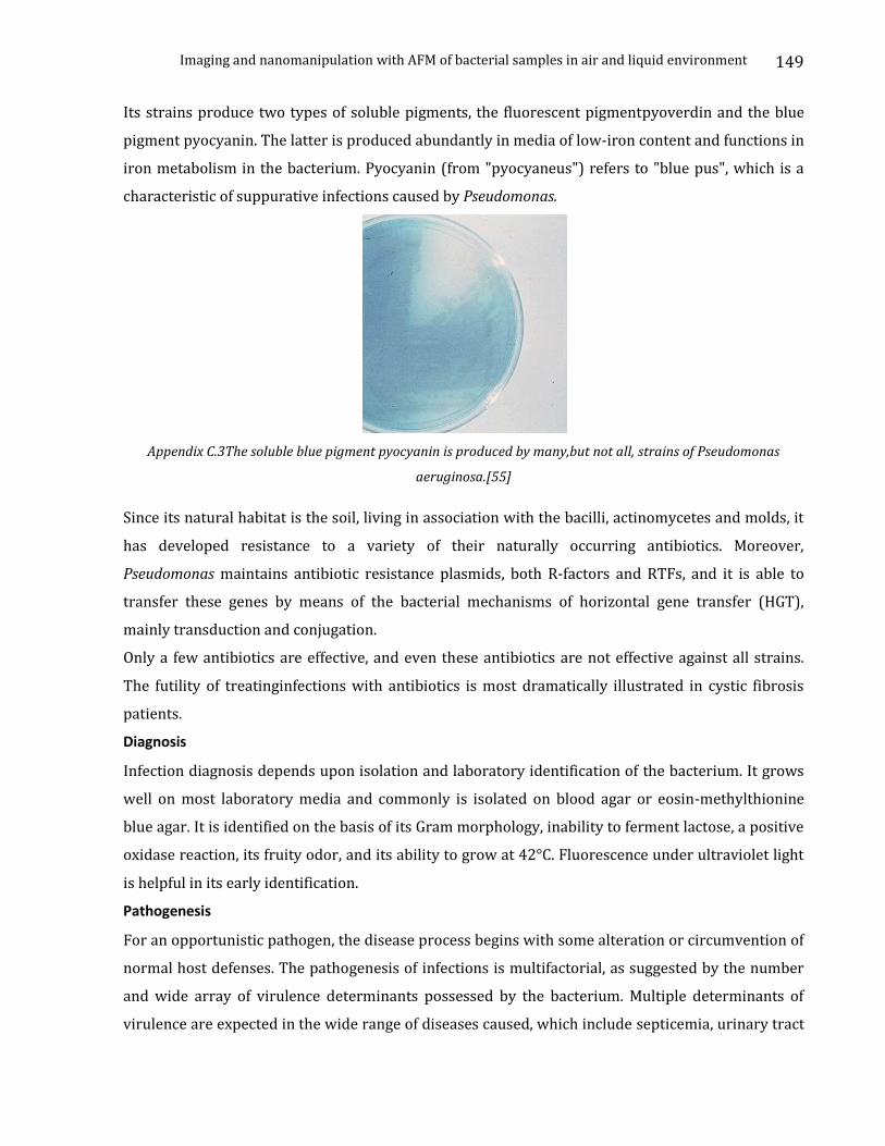
Imaging and nanomanipulation with AFM of bacterial samples in air and liquid environment
149
Its strains produce two types of soluble pigments, the fluorescent pigmentpyoverdin and the blue
pigment pyocyanin. The latter is produced abundantly in media of low-iron content and functions in
iron metabolism in the bacterium. Pyocyanin (from "pyocyaneus") refers to "blue pus", which is a
characteristic of suppurative infections caused by Pseudomonas.
Appendix C.3The soluble blue pigment pyocyanin is produced by many,but not all, strains of Pseudomonas
aeruginosa.[55]
Since its natural habitat is the soil, living in association with the bacilli, actinomycetes and molds, it
has developed resistance to a variety of their naturally occurring antibiotics. Moreover,
Pseudomonas maintains antibiotic resistance plasmids, both R-factors and RTFs, and it is able to
transfer these genes by means of the bacterial mechanisms of horizontal gene transfer (HGT),
mainly transduction and conjugation.
Only a few antibiotics are effective, and even these antibiotics are not effective against all strains.
The futility of treatinginfections with antibiotics is most dramatically illustrated in cystic fibrosis
patients.
Diagnosis
Infection diagnosis depends upon isolation and laboratory identification of the bacterium. It grows
well on most laboratory media and commonly is isolated on blood agar or eosin-methylthionine
blue agar. It is identified on the basis of its Gram morphology, inability to ferment lactose, a positive
oxidase reaction, its fruity odor, and its ability to grow at 42°C. Fluorescence under ultraviolet light
is helpful in its early identification.
Pathogenesis
For an opportunistic pathogen, the disease process begins with some alteration or circumvention of
normal host defenses. The pathogenesis of infections is multifactorial, as suggested by the number
and wide array of virulence determinants possessed by the bacterium. Multiple determinants of
virulence are expected in the wide range of diseases caused, which include septicemia, urinary tract
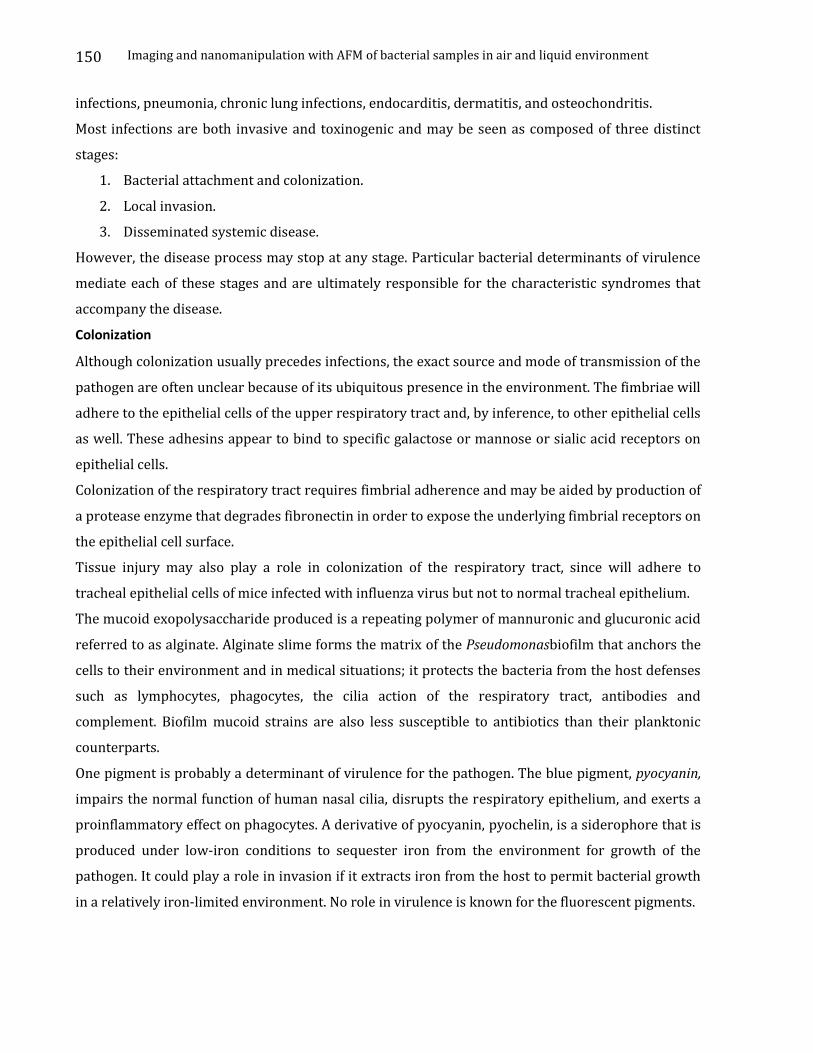
Imaging and nanomanipulation with AFM of bacterial samples in air and liquid environment
150
infections, pneumonia, chronic lung infections, endocarditis, dermatitis, and osteochondritis.
Most infections are both invasive and toxinogenic and may be seen as composed of three distinct
stages:
1. Bacterial attachment and colonization.
2. Local invasion.
3. Disseminated systemic disease.
However, the disease process may stop at any stage. Particular bacterial determinants of virulence
mediate each of these stages and are ultimately responsible for the characteristic syndromes that
accompany the disease.
Colonization
Although colonization usually precedes infections, the exact source and mode of transmission of the
pathogen are often unclear because of its ubiquitous presence in the environment. The fimbriae will
adhere to the epithelial cells of the upper respiratory tract and, by inference, to other epithelial cells
as well. These adhesins appear to bind to specific galactose or mannose or sialic acid receptors on
epithelial cells.
Colonization of the respiratory tract requires fimbrial adherence and may be aided by production of
a protease enzyme that degrades fibronectin in order to expose the underlying fimbrial receptors on
the epithelial cell surface.
Tissue injury may also play a role in colonization of the respiratory tract, since will adhere to
tracheal epithelial cells of mice infected with influenza virus but not to normal tracheal epithelium.
The mucoid exopolysaccharide produced is a repeating polymer of mannuronic and glucuronic acid
referred to as alginate. Alginate slime forms the matrix of the Pseudomonasbiofilm that anchors the
cells to their environment and in medical situations; it protects the bacteria from the host defenses
such as lymphocytes, phagocytes, the cilia action of the respiratory tract, antibodies and
complement. Biofilm mucoid strains are also less susceptible to antibiotics than their planktonic
counterparts.
One pigment is probably a determinant of virulence for the pathogen. The blue pigment, pyocyanin,
impairs the normal function of human nasal cilia, disrupts the respiratory epithelium, and exerts a
proinflammatory effect on phagocytes. A derivative of pyocyanin, pyochelin, is a siderophore that is
produced under low-iron conditions to sequester iron from the environment for growth of the
pathogen. It could play a role in invasion if it extracts iron from the host to permit bacterial growth
in a relatively iron-limited environment. No role in virulence is known for the fluorescent pigments.
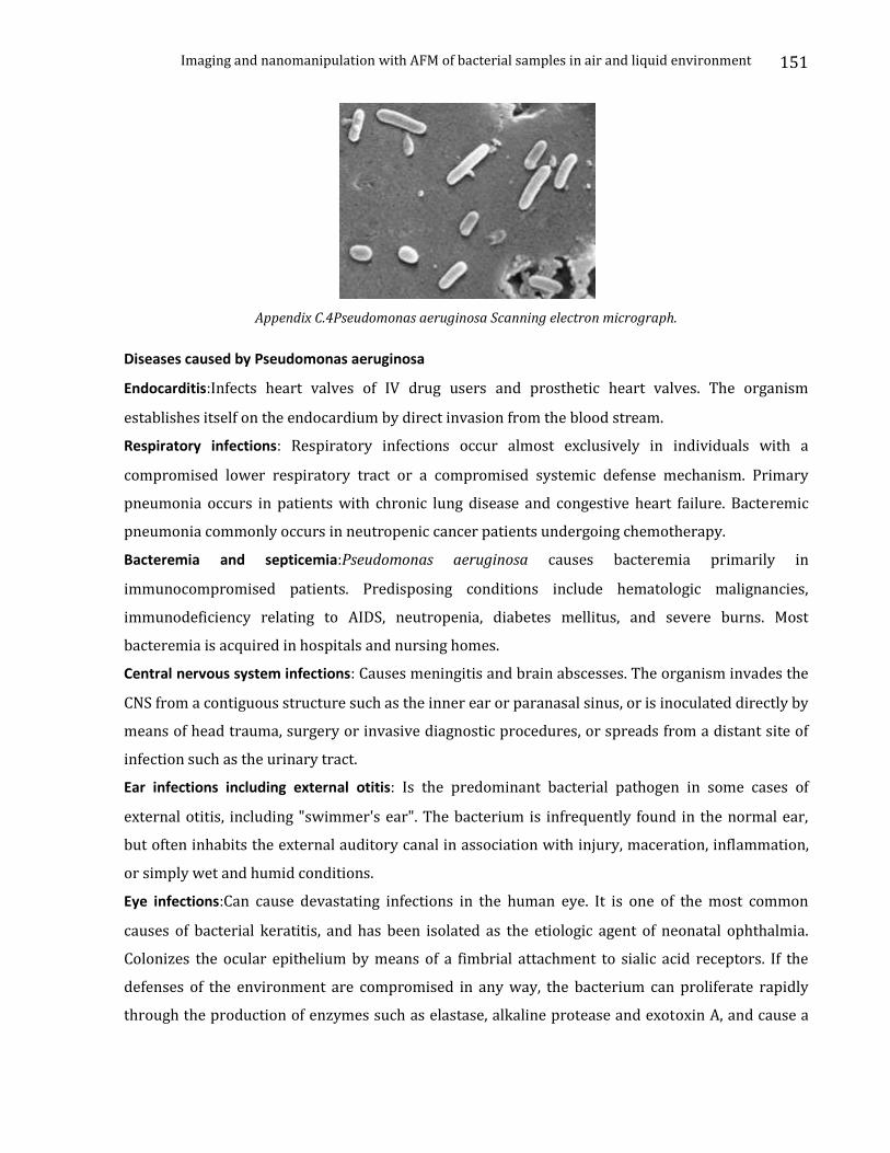
Imaging and nanomanipulation with AFM of bacterial samples in air and liquid environment
151
Appendix C.4Pseudomonas aeruginosa Scanning electron micrograph.
Diseases caused by Pseudomonas aeruginosa
Endocarditis:Infects heart valves of IV drug users and prosthetic heart valves. The organism
establishes itself on the endocardium by direct invasion from the blood stream.
Respiratory infections: Respiratory infections occur almost exclusively in individuals with a
compromised lower respiratory tract or a compromised systemic defense mechanism. Primary
pneumonia occurs in patients with chronic lung disease and congestive heart failure. Bacteremic
pneumonia commonly occurs in neutropenic cancer patients undergoing chemotherapy.
Bacteremia and septicemia:Pseudomonas aeruginosa causes bacteremia primarily in
immunocompromised patients. Predisposing conditions include hematologic malignancies,
immunodeficiency relating to AIDS, neutropenia, diabetes mellitus, and severe burns. Most
bacteremia is acquired in hospitals and nursing homes.
Central nervous system infections: Causes meningitis and brain abscesses. The organism invades the
CNS from a contiguous structure such as the inner ear or paranasal sinus, or is inoculated directly by
means of head trauma, surgery or invasive diagnostic procedures, or spreads from a distant site of
infection such as the urinary tract.
Ear infections including external otitis: Is the predominant bacterial pathogen in some cases of
external otitis, including "swimmer's ear". The bacterium is infrequently found in the normal ear,
but often inhabits the external auditory canal in association with injury, maceration, inflammation,
or simply wet and humid conditions.
Eye infections:Can cause devastating infections in the human eye. It is one of the most common
causes of bacterial keratitis, and has been isolated as the etiologic agent of neonatal ophthalmia.
Colonizes the ocular epithelium by means of a fimbrial attachment to sialic acid receptors. If the
defenses of the environment are compromised in any way, the bacterium can proliferate rapidly
through the production of enzymes such as elastase, alkaline protease and exotoxin A, and cause a
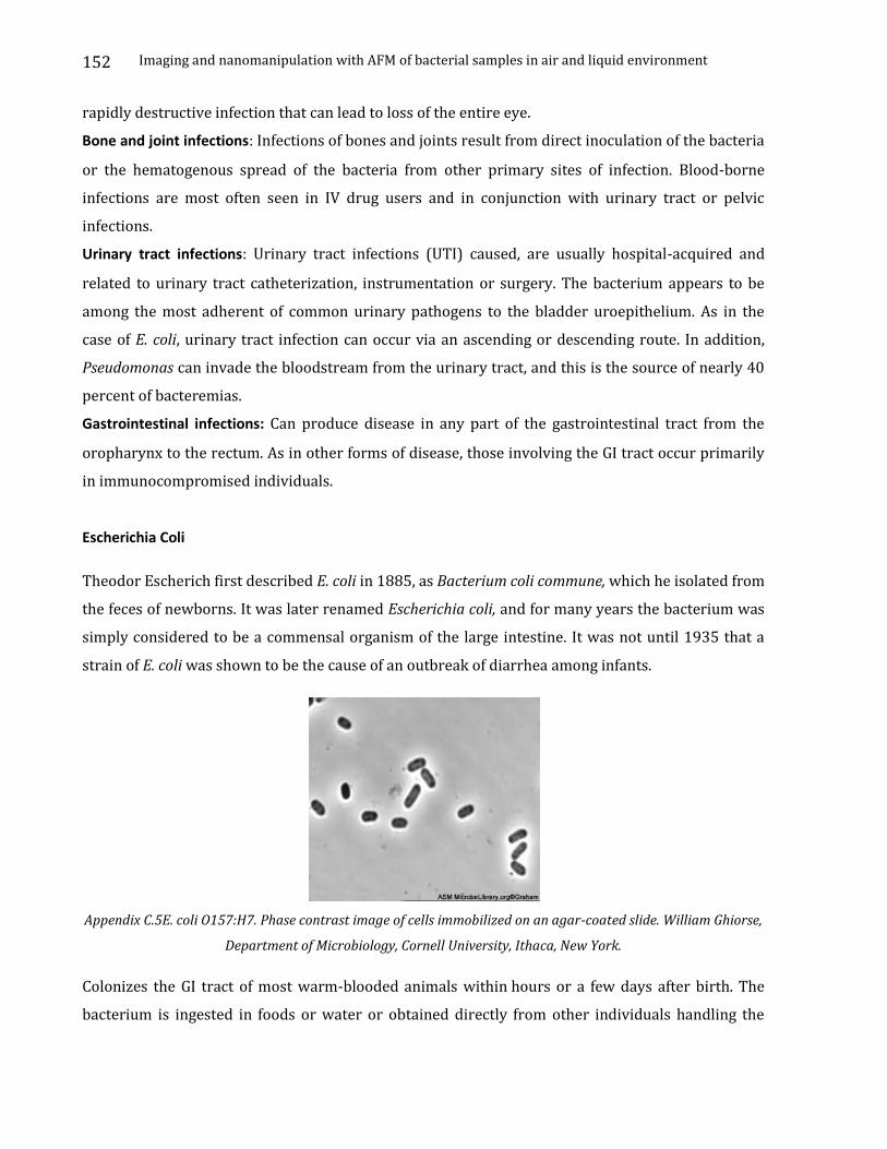
Imaging and nanomanipulation with AFM of bacterial samples in air and liquid environment
152
rapidly destructive infection that can lead to loss of the entire eye.
Bone and joint infections: Infections of bones and joints result from direct inoculation of the bacteria
or the hematogenous spread of the bacteria from other primary sites of infection. Blood-borne
infections are most often seen in IV drug users and in conjunction with urinary tract or pelvic
infections.
Urinary tract infections: Urinary tract infections (UTI) caused, are usually hospital-acquired and
related to urinary tract catheterization, instrumentation or surgery. The bacterium appears to be
among the most adherent of common urinary pathogens to the bladder uroepithelium. As in the
case of E. coli, urinary tract infection can occur via an ascending or descending route. In addition,
Pseudomonas can invade the bloodstream from the urinary tract, and this is the source of nearly 40
percent of bacteremias.
Gastrointestinal infections: Can produce disease in any part of the gastrointestinal tract from the
oropharynx to the rectum. As in other forms of disease, those involving the GI tract occur primarily
in immunocompromised individuals.
Escherichia Coli
Theodor Escherich first described E. coli in 1885, as Bacterium coli commune, which he isolated from
the feces of newborns. It was later renamed Escherichia coli, and for many years the bacterium was
simply considered to be a commensal organism of the large intestine. It was not until 1935 that a
strain of E. coli was shown to be the cause of an outbreak of diarrhea among infants.
Appendix C.5E. coli O157:H7. Phase contrast image of cells immobilized on an agar-coated slide. William Ghiorse,
Department of Microbiology, Cornell University, Ithaca, New York.
Colonizes the GI tract of most warm-blooded animals within hours or a few days after birth. The
bacterium is ingested in foods or water or obtained directly from other individuals handling the
Imaging and nanomanipulation with AFM of bacterial samples in air and liquid environment
153
infant. The human bowel is usually colonized within 40 hours of birth. Can adhere to the mucus
overlying the large intestine and once established, a strain may persist for months or years.
Resident strains shift over a long period (weeks to months), and more rapidly after enteric infection
or antimicrobial chemotherapy that perturbs the normal flora. The basis for these shifts and the
ecology in the intestine of humans are poorly understood despite the vast amount of information on
almost every other aspect of the organism's existence. The entire DNA base sequence of genome has
been known since 1997.
E. coli is the head of the large bacterial family, Enterobacteriaceae, the enteric bacteria, which are
facultatively anaerobic Gram-negative rods that live in the intestinal tracts of animals in health and
disease. A number of genera within the family are human intestinal pathogens (e.g. Salmonella,
Shigella, Yersinia). Several others are normal colonists of the human gastrointestinal tract (e.g.
Escherichia, Enterobacter, Klebsiella), but these bacteria, as well, may occasionally be associated
with diseases of humans. Physiologically, E. coli is versatile and well adapted to its characteristic
habitats. It can grow in media with glucose as the sole organic constituent. A wild type has no
growth factor requirements, and metabolically can transform glucose into all of the macromolecular
components that make up the cell. The bacterium can grow in the presence or absence of O2. Under
anaerobic conditions it will grow by means of fermentation, producing characteristic "mixed acids
and gas" as end products. However, it can also grow by means of anaerobic respiration, since it is
able to utilize NO3, NO2 or fumarate as final electron acceptors for respiratory electron transport
processes. In part, this adapts it to its intestinal (anaerobic) and its extraintestinal (aerobic or
anaerobic) habitats.
E. Coli can respond to environmental signals such as chemicals, pH, temperature, osmolarity, etc., in
a number of very remarkable ways considering it is a unicellular organism. For example, it can sense
the presence or absence of chemicals and gases in its environment and swim towards or away from
them. Or it can stop swimming and grow fimbriae that will specifically attach it to a cell or surface
receptor. In response to change in temperature and osmolarity, it can vary the pore diameter of its
outer membrane porins to accommodate larger molecules (nutrients) or to exclude inhibitory
substances. With its complex mechanisms for regulation of metabolism the bacterium can survey
the chemical contents in its environment in advance of synthesizing any enzymes that metabolize
these compounds. It does not wastefully produce enzymes for degradation of carbon sources unless
they are available, and it does not produce enzymes for synthesis of metabolites if they are available
as nutrients in the environment.

Imaging and nanomanipulation with AFM of bacterial samples in air and liquid environment
154
As a consistent inhabitant of the human intestinal tract, and it is the predominant facultative
organism in the human GI tract; however, it makes up a very small proportion of the total bacterial
content. The anaerobic Bacteroides species in the bowel outnumber E. coli by at least 20:1. However,
the regular presence of E. coli in the human intestine and feces has led to tracking the bacterium in
nature as an indicator of fecal pollution and water contamination. As such, it is taken to mean that,
wherever is found, there may be fecal contamination by intestinal parasites of humans.
Appendix C.6 Unstained cells of E. coli viewed by phase microscopy. about 1000X magnification. CDC.
Escherichia coli in the Gastrointestinal Tract
The commensal E. coli strains that inhabit the large intestine of all humans and warm-blooded
animals comprise no more than 1% of the total bacterial biomass.
Pathogenesis of E. coli
Over 700 antigenic types (serotypes) of E. coli are recognized based on O, H, and K antigens. At one
time serotyping was important in distinguishing the small number of strains that actually cause
disease. Thus, the serotype O157:H7 (O refers to somatic antigen; H refers to flagellar antigen) is
uniquely responsible for causing HUS (hemolytic uremic syndrome). Nowadays, particularly for
diarrheagenic strains (those that cause diarrhea) pathogenic E. coli are classified based on their
unique virulence factors and can only be identified by these traits. Hence, analysis for pathogenic E.
coli usually requires that the isolates first be identified as E. coli before testing for virulence
markers.
Pathogenic strains of E. coli are responsible for three types of infections in humans: urinary tract
Imaging and nanomanipulation with AFM of bacterial samples in air and liquid environment
155
infections (UTI), neonatal meningitis, and intestinal diseases (gastroenteritis). The diseases caused
(or not caused) by a particular strain of E. coli depend on distribution and expression of an array of
virulence determinants, including adhesins, invasins, toxins, and abilities to withstand host
defenses.
Appendix D
For more information over the AFM source code, matlab scripts…etc. Please contact by mail at:
Imaging and nanomanipulation with AFM of bacterial samples in air and liquid environment
156
Bibliography
Books
V. L. Marinov, Fundamentals of Scanning Probe Microscopy, (NT-MDT, 2004)
R. Howland, L. Benatar, A practical guide to Scanning Probe Microscopy
(ThermoMicroscopes, 2000)
[1] Richard Feynman - There’s Plenty of Room at the Bottom—An Invitation to Enter a New Field of
Physics. Speech, 1959. URL:http://www.its.caltech.edu/~feynman/plenty.html (January, 2008)
[2] G. Binnig, C.F. Quate, C. Gerber - Scanning Tunneling Microscopy. Phys. Rev. Lett. 56 (1986) 930.
[3] G. Binnig, H. Rohrer, Ch. Gerber, E.Weibel - Tunneling through a controllable vacuum gap. Appl.
Phys. Lett., vol. 40, p. 178 (1982).
[4] Book:V. L. Marinov, Fundamentals of Scanning Probe Microscopy, (NT-MDT, 2004)
Imaging and nanomanipulation with AFM of bacterial samples in air and liquid environment
157
[5] J. G. Simons – Generalized formula for the electric tunnel effect between similar electrodes
separated by a thin insulating film. J. Appl. Phys., 34, 1793 (1963).
[6] J. G. Simons - Electric tunnel effect between dissimilar electrodes separated by a thin insulating
film. J. Appl. Phys., 34, 2581 (1963).
[7] Atomic Force Microscopy
URL: http://www.chembio.uoguelph.ca/educmat/chm729/afm/firstpag.htm (12.08.2008)
[8] J.S.Barash - Van der Waals forces. Moscow, Nauka, 1988.
[9] Lennard-Jones, J. E. - Cohesion. Proceedings of the Physical Society, 43, 461-482 (1931).
[10] M.Saint Jean, S.Hudlet, C.Guthmann, J.Berger – Van der Waals and capacitive forces in atomic
force microscopies. J. Appl. Phys., vol. 86 (9), p. 5245 – 5248 (1999).
[11] I.A.Birger, B.F.Shorr, G.B.Iosilevich – Calculation on strength of details of machines.
Mashinostroenie, Moscow, 1979.
[12] D.Sarid - Exploring Scanning Probe Microscopy with mathematics. Wiley & Sons, 1997.
[13]A. D. L. Humphris, J. Tamayo,and M. J. Miles - Active Quality Factor Control in Liquids for Force
Spectroscopy. Langmuir, 16, 7891-7894.2000
[14]Tomás R. Rodríguez and Ricardo García - Theory of Q control in atomic force microscopy. Appl.
Phys. Lett.82, 4821 (2003); DOI:10.1063/1.1584790
[15] V. Ph. Pastushenko, P. Hinterdorfer, F. Kienberger, C. Rankl, C. Borken, G. Kada, C. Riener, H.
Schindler - Cantilever Oscillations in MAC-Mode AFM: Inertiality and Viscosity Effects of Cantilever -
Sample Interaction. Single Molecules. Vol.3 Iss.2-3 p.155-158. 2002
[16] International SPM users meeting Scientec
URL: http://usermeeting2008.scientec.fr/
[17] Nanonics
URL: http://www.nanonics.co.il/
[18] SCIENTEC
URL: http://www.scientec.fr/
[19] NanoSurf
URL:http://www.nanosurf.com/

Imaging and nanomanipulation with AFM of bacterial samples in air and liquid environment
158
[20] Nanotec Electrónica
URL:http://www.nanotec.es/
[21] C. V. Raman, K. S. Krishnan - A New Type of Secondary Radiation Nature121, 501-502 (31
March 1928)
[22] Manfred von Ardenne, Manfred (1938b). "Das Elektronen-Rastermikroskop. Praktische
Ausführung" (in German). Zeitschrift für technische Physik19: 407–416.
[23] [3.14] Futamoto, Masaaki et al., - Development of Technologies for 2-Gb/in2 Areal Density
Recording. Electronics and Communications in Japan, Part II-Electronics, vol. 76, No. 3 (Mar. 1993)
pp. 94-103
[24] T. Acsente - Laser diode intensity noise induced by mode hopping. Romanian Reports in Physics,
Vol. 59, No. 1, P. 87–92, 2007
[25] H. Edwards, L. Taylor, W. Duncan and A. J. Melmed. Fast, high-resolution atomic force
microscopy using a quartz tuning fork as actuator and sensor. J. Appl. Phys. 82 (3), 1997.
[26] W. H. J. Rensen, N. F. van Hulst,S. B. Kämmer - Imaging soft samples in liquid with tuning fork
based shear force microscopy. Appl. Phys. Lett. 77, 1557 (2000).
[27] M. Koopman, B. I. de Bakker, M. F. Garcia-Parajo, and N. F. van Hulst - Shear force imaging of
soft samples in liquid using a diving bell concept. Appl. Phys. Lett. 83, 24 (2003)
[28] Agilent Technologies.
URL:http://www.home.agilent.com/agilent/home.jspx?cc=US&lc=eng&cmpid=5443 (24.08.2008)
[29] Aist-Nt
URL: http://www.aist-nt.com/ (24.08.2008)
[30] Asylum Research
URL: http://www.asylumResearch.com/ (24.08.2008)
[31] Veeco
URL:http://www.veeco.com/Products/metrology_and_instrumentation/AFM_SPM/index.aspx
(24.08.2008)
[32] Angstrom Advanced Inc.
Imaging and nanomanipulation with AFM of bacterial samples in air and liquid environment
159
URL: http://www.angstrom-advanced.com/ (April 2008)
[33] JPK Instruments
URL: http://www.jpk.com/index.2.html (May 2008)
[34] Tomás R. Rodríguez and Ricardo García. Theory of Q control in atomic force microscopy.Appl.
Phys. Lett. 82, 4821 (2003)
[35] Q Control
URL:http://www.nanoanalytics.com/en/hardwareproducts/qcontrol/howitworks/index.php
[36] Q Control application from Nanoscience Instruments
URL: http://www.nanoscience.com/products/qcontrol_applications.html
[37] NT-MDT
URL: http://www.ntmdt.com/ (June 2008)
[38] Omicron
URL: http://www.omicron.de/ (May 2008)
[39] Pacific Nanotechnology
URL: http://www.pacificnanotech.com/ (June 2008)
[40] Park Systems
URL: http://www.parkafm.com/New_html/main.php(Agust 2008)
[41] RHK Technology
URL: http://www.rhk-tech.com/scanhead.php (July 2008)
[42] Surface Imaging Systems
URL: http://www.surface-imaging.com/ (Agust 2008)
[43] Gnome X Scanning Microscopy project
URL: http://gxsm.sourceforge.net/ (September 2007)
[44] The GNOME desktop environment
URL: http://www.gnome.org (Miguel de Icaza).
[45] TMS320C32 of Texas Instruments (Newer version available)
URL: http://focus.ti.com/docs/prod/folders/print/tms320c32.html (January 2008)
[46] N. Banning, S. Toze and B. J. Mee -Persistence of biofilm-associated Escherichia coli and
Pseudomonas aeruginosa in groundwater and treated effluent in a laboratory model system.
Microbiology 149, 47-55 (2003).
Imaging and nanomanipulation with AFM of bacterial samples in air and liquid environment
160
[47] G. Yang, S. H. Leuba, C. Bustamante, J. Zlatanove, K. Holde- Role of linker histones in extended
chromatin fibre structure.Nature Structural Biology1,761-763 (1994)
[48] Carlos Bustamante, Claudio Rivetti, David J Keller - Scanning force microscopy under aqueous
solutions. Current Opinion in Structural BiologyVolume 7, Issue 5, Pages 709-716,October 1997.
[49] Matthias Rief, Mathias Gautel, Filipp Oesterhelt, Julio M. Fernandez, Hermann E. Gaub -
Reversible Unfolding of Individual Titin Immunoglobulin Domains by AFM.Science Vol.276 no.
5315, pp. 1109 – 1112, 16 May 1997.
[50] D. J. Müller, D. Fotiadis, S. Scheuring, Sh. A. Müller, A. Engel - Electrostatically balanced sub-
nanometer imaging of biological specimens by AFM. Biophysical Journal. Volume 76, 1101–1111,
February 1999.
[51] F. Moreno-Herrero, J. Colchero,J. Gómez-Herrero,A. M. Baró - Atomic force microscopy contact,
tapping, and jumping modes for imaging biological samples in liquids. Physical Review. 69, 2004.
[52] NISE Network
URL: http://www.nisenet.org/publicbeta/articles/seeing_atoms/index.html (12.08.2008)
[53] www.wikipedia.com (November, 2007)
[54] Pseudomonas aeruginosas (September 4, 2008)
URL:http://www.textbookofbacteriology.net/pseudomonas.html
[55] Escherichia Coli (September 4, 2008)
URL:http://www.textbookofbacteriology.net/e.coli.html
[56] WikipediaURL: http://www.wikipedia.org/ (September 4, 2008)
[57] Liwei Chen, Xuechun Yu, Dan Wang. - Cantilever dynamics and quality factor control in AC
mode AFMheight measurements. Ultramicroscopy, 107, 275–280 (2007)
[58] Y. Z. Liu, S. H. Leuba, S. M. Lindsay -Relationship between Stiffness and Force in
Single Molecule Pulling Experiments. Langmuir, 15, 8547-8548, 1999.
[59] P. Zahl, M. Bierkandt, S. Schröder - The flexible and modern open source scanning probe
microscopy software package GXSM. Review of scientific instruments, Vol.74-3 (2003).
[60] William F. Heinz and Jan H. Hoh - Spatially resolved force spectroscopy of biological surfaces
using the atomic force microscope. Nanotechnology,Vol. 17, (1999)
[61] S. M. Deupree, M. H. Schoenfisch - Quantitative Method for Determining the Lateral Strength of
Bacterial Adhesion and Application for Characterizing Adhesion Kinetics. Langmuir 2008, 24, 4700.
Imaging and nanomanipulation with AFM of bacterial samples in air and liquid environment
161
[62] R. J. Cannara, M. Eglin, R. W. Carpick -Lateral force calibration in atomic forcemicroscopy: A
new lateral forcecalibration method and generalguidelines for optimization. Review of Scientific
Instruments 77, 053701 (2006)
[63] Elena T. Herruzo and Ricardo Garcia - Frequency response of an atomic force microscope in
liquids and air: Magnetic versus acoustic excitation. Applied Physics Letters91, 143113 (2007)
[64] A. Asenjo, M. Jaafar - Dislocation mechanisms in the first stage of plasticity of nanoindented Au
(111) surfaces. Physical Review B 73, 075431 (2006)


![[49] Single-Molecule DNA Nanomanipulation: Detection of](https://img.pdfslide.net/doc/110x75/617358589073e71ea24d792e/49-single-molecule-dna-nanomanipulation-detection-of-.jpg)