IMEX Schemes for Advection-Diffusion EquationsDoktorandenseminar WS 14/15

Serena Keller

Institute of Aerodynamics and Gas Dynamics, University Stuttgart

27. January 2015

Outline

Motivation

Stability Conditions for Advection-Diffusion EquationsExplicit RKIMEX RK

IMEX Runge-Kutta SchemeAlgorithm

Benchmark ProblemsSinus Transport in 2DSingular Perturbation Problem in 1D

Summary - Outlook

Motivation

I Explicit Scheme: Time step restriction due to stabilityconditions

I IMEX schemes: Weaker time step restriction(Implicit discretization of the diffusion part)

⇒ Usage of greater time steps⇒ Saving computing time

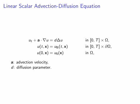
Linear Scalar Advection-Diffusion Equation

ut + a · ∇u = d∆u in [0,T ]× Ω,

u(t, x) = uB(t, x) in [0,T ]× ∂Ω,

u(0, x) = u0(x) in Ω,

a: advection velocity,d : diffusion parameter.

Stability Conditions of Explicit Schemes

For explicit time discretizations the following stability conditionshave to be satisfied:

|a|∆t

∆x< 1

d∆t

∆x2<

1

2.

Thus ∆t has to be chosen so that

∆t < min

∆x

|a|,

∆x2

2d

.

Stability Condition of IMEX Runge-Kutta Schemes

The idea of IMEX (Implicit-Explicit) schemes is to dispose of thediffusion stability condition

H

HHHHH

d∆t

∆x2<

1

2.

by discretizing the diffusion part F d(u) := d∆u implicitly and theadvective part F a(u) := −a · ∇u explicitly :

ut = F a(u) + F d(u).

So the convection stability condition remains:

|a|∆t

∆x< 1.

IMEX Algorithm

ut = F a(u) + F d(u).

Explicit

F a(u) := −a · ∇u

Butcher Tables:

A, b and c of an explicit(s + 1)-stage ERK

Implicit

F d(u) := d∆u

Butcher Tables:

A =

[0 0∗ A

], b =

[0b

]and

c =

[0c

].

A, b and c are the Butchertables of a s-stage DIRK

IMEX Algorithm

Let un be given and un+1 wanted.

1 k1 = Fd (tn, un)

2 k1 = F a(tn, un)

3 DO i=2,...σ

4 Solve for ki : ki = Fd (tn + ci∆t, ui )

with ui = un + ∆t (∑i

j=1 aij kj +∑i−1

j=1 aij kj )5 Evaluate ki : ki = F a(tn + ci∆t, ui )

6 END DO

7 un+1 = un + ∆t (∑σ

j=1 bj kj +∑σ

j=1 bj kj )

Implicit equation:

ki = F d(tn + ci∆t, un + ∆t

( i∑j=1

aij kj +i−1∑j=1

aij kj))

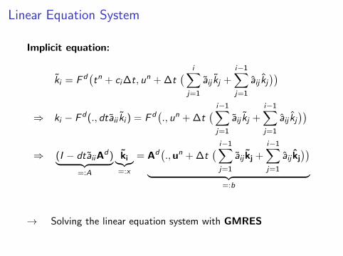
Linear Equation System

Implicit equation:

ki = F d(tn + ci∆t, un + ∆t

( i∑j=1

aij kj +i−1∑j=1

aij kj))

⇒ ki − F d(., dtaii ki ) = F d(., un + ∆t

( i−1∑j=1

aij kj +i−1∑j=1

aij kj))

⇒ (I − dtaiiAd)︸ ︷︷ ︸

=:A

ki︸︷︷︸=:x

= Ad(.,un + ∆t

( i−1∑j=1

aij kj +i−1∑j=1

aij kj))

︸ ︷︷ ︸=:b

→ Solving the linear equation system with GMRES

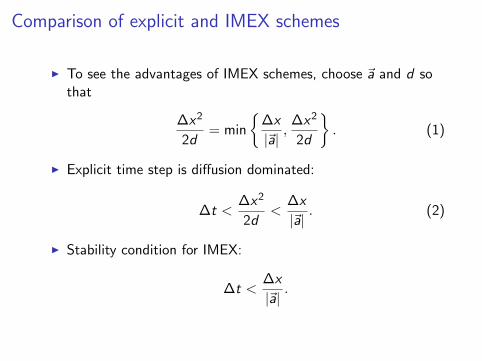
Comparison of explicit and IMEX schemes

I To see the advantages of IMEX schemes, choose ~a and d sothat

∆x2

2d= min

∆x

|~a|,

∆x2

2d

. (1)

I Explicit time step is diffusion dominated:

∆t <∆x2

2d<

∆x

|~a|. (2)

I Stability condition for IMEX:

∆t <∆x

|~a|.

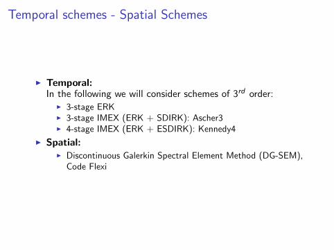
Temporal schemes - Spatial Schemes

I Temporal:In the following we will consider schemes of 3rd order:

I 3-stage ERKI 3-stage IMEX (ERK + SDIRK): Ascher3I 4-stage IMEX (ERK + ESDIRK): Kennedy4

I Spatial:I Discontinuous Galerkin Spectral Element Method (DG-SEM),

Code Flexi

Sinus Transport in 2DI Exact solution of the linear scalar advection-diffusion equation

in 2D

u(x , y , t) = sin(ω(x − a1 − t)) sin(ω(y − a2 − t))e−2dω2t .

where ~a = (a1, a2) = (1, 1).

CoordinateX

Co

ord

inat

eY

-1 -0.5 0 0.5 1-1

-0.5

0

0.5

1

Solution

0.90.80.70.60.50.40.30.20.10

-0.1-0.2-0.3-0.4-0.5-0.6-0.7-0.8-0.9

t=0

CoordinateX

Co

ord

inat

eY

-1 -0.5 0 0.5 1-1

-0.5

0

0.5

1

Solution

0.90.80.70.60.50.40.30.20.10

-0.1-0.2-0.3-0.4-0.5-0.6-0.7-0.8-0.9

t=2

CoordinateX

Co

ord

inat

eY

-1 -0.5 0 0.5 1-1

-0.5

0

0.5

1

Solution

0.90.80.70.60.50.40.30.20.10

-0.1-0.2-0.3-0.4-0.5-0.6-0.7-0.8-0.9

t=4

CoordinateX

Co

ord

inat

eY

-1 -0.5 0 0.5 1-1

-0.5

0

0.5

1

Solution

0.90.80.70.60.50.40.30.20.10

-0.1-0.2-0.3-0.4-0.5-0.6-0.7-0.8-0.9

t=6

Parameter Standard ValuesType of nodes Gauss

Polynomial Order 8Mesh size 8x8

εGMRES truncation 10−4

d

Comparison of Explicit and IMEX schemes

d

tim

e st

ep

10-2 10-1 100 101 10210-7

10-6

10-5

10-4

10-3

10-2

Explicit ERK3IMEX Ascher3IMEX Kennedy4

d

L2

erro

r

10-2 10-1 100 101 10210-18

10-16

10-14

10-12

10-10

10-8

10-6

10-4

Explicit ERK3IMEX Ascher3IMEX Kennedy4

d

CP

U t

ime

10-2 10-1 100 101 10210-1

100

101

102

103

Explicit ERK3IMEX Ascher3IMEX Kennedy4

Singular Perturbation Problem in 1D

I Singular Perturbation Problem (SPP) can be seen as a modelfor the formation of a boundary layer

I Consider the linear scalar advection diffusion equation in 1Dwith a singular perturbation of the boundary values:

ut + a ux = d uxx in [0,T ]× [0, 1],

u(0, t) = 0 in [0,T ],

u(1, t) = 1 in [0,T ],

u(x , 0) = u0(x) in [0, 1].

I Consider the stationary limit of the problem with a = −1.∣∣∣‖uh(tn+1)− uex‖L2([0,1]) − ‖uh(tn)− uex‖L2([0,1])

∣∣∣ < c .

x

u

0 0.2 0.4 0.6 0.8 10

0.2

0.4

0.6

0.8

1

d=0.075d=0.1d=0.115

Parameter Standard ValuesType of nodes Gauss

Polynomial Order 8Mesh size 8

εGMRES truncation 10−2

Stationary truncation c 10−12

Comparison of Explicit and IMEX schemes

d

tim

e st

ep d

t

0.025 0.05 0.075 0.110-4

10-3

10-2

Explicit ERK3IMEX Ascher3IMEX Kennedy4

d

L2

erro

r

0.01 0.03 0.05 0.07 0.09 0.11 0.1310-8

10-7

10-6

10-5

10-4

10-3

10-2

Explicit ERK3IMEX Ascher3IMEX Kennedy4

d

CP

U t

ime

0.01 0.03 0.05 0.07 0.09 0.11 0.13

5

10

15

20 Explicit ERK3IMEX Ascher3IMEX Kennedy4

Summary

I For the Sinus transport: Kennedy4 and Ascher3 are fasterthan the explicit scheme, but less accurate.

I For the convergence to the stationary limit: Kennedy4 is thefastest scheme

I Although Kennedy4 has 4 stages, it needs less or the sametime than Ascher3 with the same L2 accuracy for theconsidered test cases

Outlook

I Preconditioning of the implicit part

I Implementing IMEX schemes for Navier Stokes with a nonlinear solver (Newton)