Immigration, Matching, and Inequality

Jaerim Choi Jihyun ParkUniversity of California, Davis KISDI

March 2017

Abstract

What are the distributional impacts of immigration on native workers? To an-swer this question, we develop a model of worker-establishment matching with a log-supermodular production function and study the impact of low-skilled immigration onnative workers where immigration is defined as a matching between immigrant workersand establishments. Immigration will increase the relative supply of workers, inten-sifying competition among workers within establishment, and thereby reducing wagespaid to native workers (matching ratio channel). However, native workers are nowpushed up to be matched with establishment with higher productivity, which leadsto an increase in wages for native workers (matching quality channel). The modelpredicts that inequality among native workers widens as more skilled native workersbenefit more from this re-matching. Using Census and IPUMS American CommunitySurvey over the period 1980-2010, we test the model’s predictions by exploiting thevariation of stock of immigration across commuting zone-year. We demonstrate thatthe immigration increases inequality among native workers in the local labor marketsas predicted by the model. Next, to test the matching quality channel, we decomposeworker’s wage into components related to observable worker characteristics, establish-ment heterogeneity, other unobservable fixed effects, and residual variation. Using theestimated establishment heterogeneity as a proxy for native worker’s matching counter-parts, we find that immigration induces native workers to match with more productiveestablishment.

Jaerim Choi, Department of Economics, University of California, Davis, jrchoi@ucdavis.edu,Jihyun Park, Korea Information Society Development Institute, jhnpark@kisdi.re.kr

1

1. Introduction

What are the distributional effects of immigration in the U.S.? This paper proposes a

new framework, a matching between workers and establishments, to think about the impacts

of immigration on inequality.

Immigrants in the U.S. labor market are characterized by bimodal skill distribution -

there are relatively more immigrants at the higher and lower end of the skill distribution.

Also, in terms of tasks, immigrants are relatively more specializing in production tasks

than establishmential tasks (Peri and Sparber, 2009). Thus, the influx of immigrants may

differently affect natives with heterogeneous skills and heterogeneous tasks, which leads to a

change on inequality in the U.S. Therefore, it is essential to incorporate heterogeneous skills

and tasks into the theortical immigration model, not based on representative agent model,

to analyze the impact of immigration on inequality. In addition to heterogeneity in inflows

of immigrants, U.S. labor markets are characterized by positive assortative matching (PAM)

between workers and establishments and both log salary function and log wage function are

increasing and convex in education levels (Lemieux, 2006, 2008). This leads us to specify

log supermodular production function in the model to replicate these two observations.

Based on the observations in the U.S. labor market, we build a theoretical immigration

framework with a matching between heterogeneous workers and heterogeneous establish-

ments in which the production function is log supermodular. In the model, immigration

changes the factor endowment and factor distribution in the local labor market, which leads

to the change in matching between workers and establishments. The model predicts that im-

migrant inflow would affect both the match ratio (the number of workers per establishment)

and the match quality (the skill level of matching counterparts). This would differently im-

pact natives with different skill levels and tasks. For instance, influx of low-skilled immigrants

can increase the match ratio, which generates competition effect for native workers, thereby

lowering wages for native workers. However, native workers can be paired up with estab-

lishments with higher skills, which leads to increases in wages for native workers. Moreover,

the model predicts that inequality within native workers rises with the inflow of low-skilled

immigrants as better workers benefit more through the increase in match quality due to the

assumption of log supermodular production function.

After explaining the theoretical framework, we empirically test whether the theory applies

to the U.S. local labor markets in 1980-2010. Especially, we focus on the inflow of low-skilled

immigration as foreing-born share of the U.S. population by less educated group (high-

school or less) is overrepresented than other groups (Peri, 2016) and the absolute number of

immigrants in this group outweighs the number of other groups. Thus, it is easy to identify

1

low-skilled immigration in the data. To implement empirical procedure, we construct a

shift-share instrument for the stock of low-skilled immigrants. Using this instrument, we

demonstrate that the influx of low-skilled immigrants increases the relative supply of workers

(matching ratio channel) and induces native workers to match with more able native-born

establishments (matching quality channel) in the local labor markets. Combining these two

channels, the distributional impacts of the influx of low-skilled immigration in the U.S. are

heterogeneous across different skills of native workers. Especially, inequality among native-

born workers widens as more skilled workers benefit more from re-matching in the local labor

markets.

This research contributes to three strands of literature. First, there is a rich literature on

the impact of immigrants on wages in the destination country. Previous studies have shown

mixed results, and researchers investigated various channels – such as complementarity, sub-

stitutability, and specialization – that immigrants can affect natives. This study introduces

a novel channel, a matching between workers and establishments, to the literature. Our

theory and empirical work supports that workers with heterogeneous skills can be differen-

tially affected by the influx of low-skilled immigration through the changes in the matching

between workers and establishments in the local labor market. Second, we contribute to

the immgration literature by studying the effect of immigration on inequality. As many of

previous research only focus on the average wage of native workers, we expand the scope

of the impact of immigration on local labor market by exploring inequality consequences of

immigration. Third, there is an extensive literature on the effect of trade on inequality using

assignment model with heterogeneous worker framework. To the best of our knowledge, this

paper is the first application of assignment model to the immigration literature.

The remainder of this paper is organized as follows. Section 2 provides an overview of the

related literature and Section 3 provides some observations in the U.S. labor market. Sec-

tion 4 presents the theoretical model. Section ?? presents numerical simulations. Section 6

tests whether the model fits to the local labor markets in the U.S., and Section 7 concludes.

2. Previous Literature

There has been an extensive literature on the effect of immigrants on the wages of natives

(Borjas, 2003; Card, 2009; Ottaviano and Peri, 2012; Basso and Peri, 2015). However,

studies in this research arena have not come to a unique conclusion as to the direction

of the impact of immigration on the wages of native workers. Borjas (2003) argues that

immigration adversely affects the wages of competing native workers. The author assumes

that workers with same education and different work experience in a national market are

2

not perfect substitutes and uses this variations in schooling-experience groups to measure

the wage impact of immigration. This study adopts national-level approach, instead of

exploiting differences in local labor markets, because the latter approach is problematic in

that immigrants can move across cities and regions. On the contrary, Ottaviano and Peri

(2012) find a small positive effect on native wages. Using the national approach as in Borjas

(2003), this study estimates elasticity of substitution across different group of workers and

uses the estimated elasticities to calculate the total wage effect of immigration. They find

a small but significant degree of imperfect substitutability between natives and immigratns

under the same education-experience cell, which leads to the overall positive wage effect of

immigration. Similar to Ottaviano and Peri (2012), Basso and Peri (2015) find a zero to

positive effect of immigration on the wages of native workers using 2SLS method with a

shift-share instrument. Card (2009) explores the impact of immigration on wage inequality

using cross-city variations in the U.S. The author finds that immigration had small impact

on wage inequality among natives. However, considering immigrants are counted in total

population, the effect of immigration on total wage inequality becomes positive as immigrants

tend to locate in the upper and lower tails of the skill distribution. We contribute to this

literature by building a new immigration framework to analyze the impact of immigration

on the wages and inequality of native workers. The model framework bases on two tasks

(establishments and workers) with continuum of skills which allows us to analyze diverse

aspects of immigration on natives. Rich predictions from the model sheds some light on the

impact of immigration on the wages of native workers, which is a hotly debated topic in this

literature.

Researchers have also studied more micro-founded mechanisms for the impact of immi-

gration on the wages of native-born workers. Peri and Sparber (2009) argue that native-born

workers and foreign-born workers specialize in different production tasks so that large influx

of less-educated immigrants may not necessarily substitute less-educated native workers. In

the model, immigration will re-allocate task supply in which foreign-born workers would

specialize in manual tasks while native workers would specialize in communication tasks.

The task specialization mechanism attenuates negative wage impact of immigration on na-

tive workers. Hunt and Gauthier-Loiselle (2010) find an evidence of the positive spillovers of

skilled immigration on boosting innovation in the U.S. As immigrants are more concentrated

in science and engineering occupations than natives in those occupations, immigrants increase

innovation as measured by US patents per capital. Since scientific and engineering knowledge

transfers occur easily, this positive spillover makes native workers better off. Ortega and Peri

(2014) show that openness to immigration leads to higher income per capita. This positive

effect operates through an increased total factor productivity from increased diversity and

3

ideas in the host country. We introduce a new mechanism, “worker-establishment matching”

and complementary effect between two, to explain the effect of immigrants on the natives.

As immigration can be seen as a matching between immigrants and natives, we incorporate

matching framework into the model and analyze how different types of immigration affect

the matching function in the host country. Through the change in the matching function

and relative factor endowments from immigration, native workers are paired up with new

establishments, thereby affecting the wages of native workers and inequality among native

workers.

Our insight on immigration, defined as a matching between immigrants and natives, is

adopted from the concept of globalization in Kremer and Maskin (1996, 2006). Kremer and

Maskin (1996) propose a model of production by workers of different skills with comple-

mentarity between two tasks. In a closed economy setting, they argue that segregation of

high-skilled and low-skilled workers into separate firms will lead to wage inequality. Kre-

mer and Maskin (2006) extend the analysis to a two-country framework and analyze the

impact of globalization, which is defined as workers from different countries being able to

form a team in the same firm. Globalization enables high-skilled workers in poor countries

to be matched with more skilled workers in rich countries. Low skilled workers in the poor

countries are marginalized due to globalization because their skill levels are so low that rich

country workers do not want to match with them.

Our theoretical framework is also closely related to the burgeoning literature in interna-

tional trade that uses an assignment model with heterogeneous workers (Antras et al., 2006;

Ohnsorge and Trefler, 2007; Costinot and Vogel, 2010; Grossman et al., 2013; Choi, 2016).

Antras et al. (2006) propose a knowledge-based hierarchy model to analyze the impact of

cross-counry team formation on the structure of wages. Ohnsorge and Trefler (2007) study

the implication of two-dimensional worker heterogeneity and worker sorting on international

trade. Costinot and Vogel (2010) develops tools and techniques to analyze the factor allo-

cation and factor prices in a Roy-like assignment model with a continuum of workers and

a contiuum of tasks. Grossman et al. (2013) develop one country, two industries and two

heterogeneous factors of production framework in which they study the distributional ef-

fects of international trade. Choi (2016) extends Grossman et al. (2013)’s framework to two

countries to analyze the distributional impact of offshoring on heterogeneous agents in each

country. In this paper, we base our model upon Grossman et al. (2013) and Choi (2016)’s

framework and extend it to incorporate two population groups (immigrants and natives) and

analyze the distributional impact of immigration on native workers. The theoretial model

develped in this paper, to the best of our knowledge, is the first application of the assignment

model with heteregeneous workers in immigration literature.

4

3. Some Observations in the U.S. Labor Market

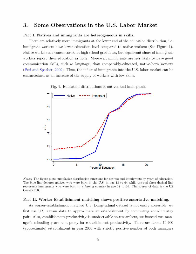
Fact I. Natives and immigrants are heterogeneous in skills.

There are relatively more immigrants at the lower end of the education distribution, i.e.

immigrant workers have lower education level compared to native workers (See Figure 1).

Native workers are concentrated at high school graduates, but significant share of immigrant

workers report their education as none. Moreover, immigrants are less likely to have good

communication skills, such as language, than comparably-educated, native-born workers

(Peri and Sparber, 2009). Thus, the influx of immigrants into the U.S. labor market can be

characterized as an increase of the supply of workers with low skills.

Fig. 1. Education distributions of natives and immigrants

Notes: The figure plots cumulative distribution functions for natives and immigrants by years of education.The blue line denotes natives who were born in the U.S. in age 18 to 64 while the red short-dashed linerepresents immigrants who were born in a foreing country in age 18 to 64. The source of data is the USCensus 2000.

Fact II. Worker-Establishment matching shows positive assortative matching.

As worker-establishment matched U.S. Longitudinal dataset is not easily accessible, we

first use U.S. census data to approximate an establishment by commuting zone-industry

pair. Also, establishment productivity is unobservable to researchers, we instead use man-

ager’s schooling years as a proxy for establishment productivity. There are about 19,400

(approximate) establishment in year 2000 with strictly positive number of both managers

5

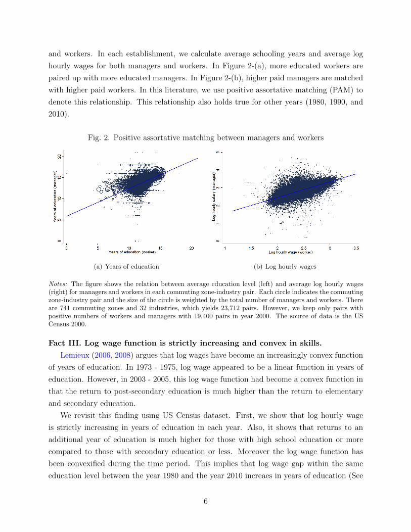
and workers. In each establishment, we calculate average schooling years and average log

hourly wages for both managers and workers. In Figure 2-(a), more educated workers are

paired up with more educated managers. In Figure 2-(b), higher paid managers are matched

with higher paid workers. In this literature, we use positive assortative matching (PAM) to

denote this relationship. This relationship also holds true for other years (1980, 1990, and

2010).

Fig. 2. Positive assortative matching between managers and workers

(a) Years of education (b) Log hourly wages

Notes: The figure shows the relation between average education level (left) and average log hourly wages(right) for managers and workers in each commuting zone-industry pair. Each circle indicates the commutingzone-industry pair and the size of the circle is weighted by the total number of managers and workers. Thereare 741 commuting zones and 32 industries, which yields 23,712 pairs. However, we keep only pairs withpositive numbers of workers and managers with 19,400 pairs in year 2000. The source of data is the USCensus 2000.

Fact III. Log wage function is strictly increasing and convex in skills.

Lemieux (2006, 2008) argues that log wages have become an increasingly convex function

of years of education. In 1973 - 1975, log wage appeared to be a linear function in years of

education. However, in 2003 - 2005, this log wage function had become a convex function in

that the return to post-secondary education is much higher than the return to elementary

and secondary education.

We revisit this finding using US Census dataset. First, we show that log hourly wage

is strictly increasing in years of education in each year. Also, it shows that returns to an

additional year of education is much higher for those with high school education or more

compared to those with secondary education or less. Moreover the log wage function has

been convexified during the time period. This implies that log wage gap within the same

education level between the year 1980 and the year 2010 increaes in years of education (See

6

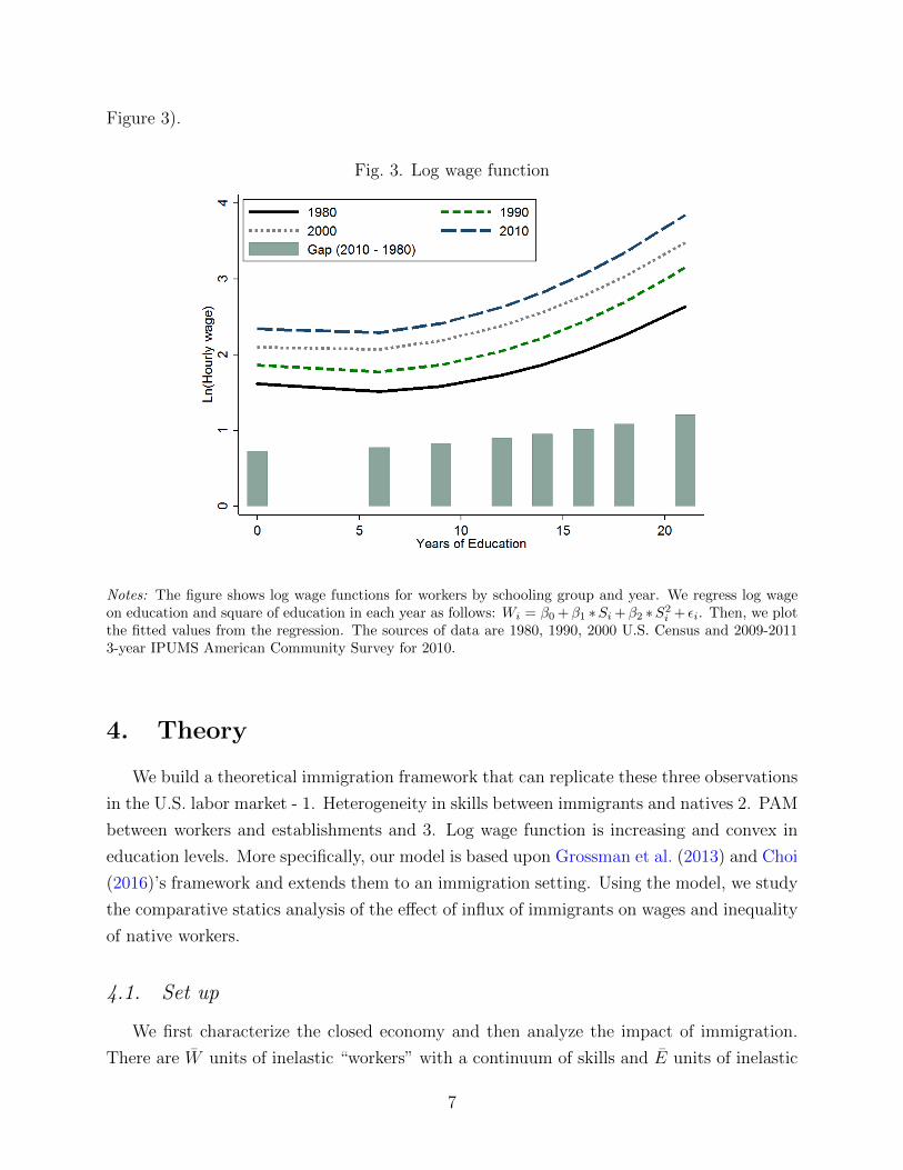
Figure 3).

Fig. 3. Log wage function

Notes: The figure shows log wage functions for workers by schooling group and year. We regress log wageon education and square of education in each year as follows: Wi = β0 +β1 ∗Si +β2 ∗S2

i + εi. Then, we plotthe fitted values from the regression. The sources of data are 1980, 1990, 2000 U.S. Census and 2009-20113-year IPUMS American Community Survey for 2010.

4. Theory

We build a theoretical immigration framework that can replicate these three observations

in the U.S. labor market - 1. Heterogeneity in skills between immigrants and natives 2. PAM

between workers and establishments and 3. Log wage function is increasing and convex in

education levels. More specifically, our model is based upon Grossman et al. (2013) and Choi

(2016)’s framework and extends them to an immigration setting. Using the model, we study

the comparative statics analysis of the effect of influx of immigrants on wages and inequality

of native workers.

4.1. Set up

We first characterize the closed economy and then analyze the impact of immigration.

There are W units of inelastic “workers” with a continuum of skills and E units of inelastic

7

“establishments” with a continuum of productivities. Workers are indexed by their skill level

zW ∈ W ⊂ R++ and establishments are indexed by their productivity level zE ∈ E ⊂ R++.

The probability density functions for workers and establishments, φW (zW ) and φE(zE), are

both continuous and strictly positive on the compact subsets, W = [zW,min, zW,max] and

E = [zE,min, zE,max].

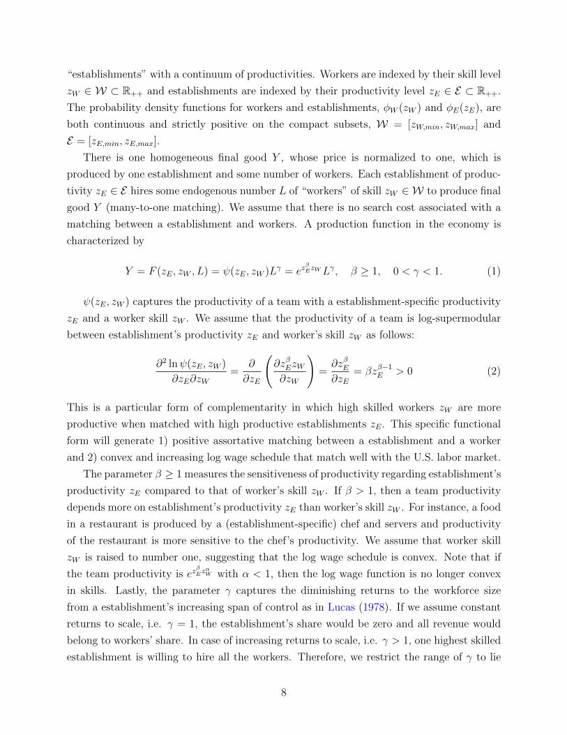
There is one homogeneous final good Y , whose price is normalized to one, which is

produced by one establishment and some number of workers. Each establishment of produc-

tivity zE ∈ E hires some endogenous number L of “workers” of skill zW ∈ W to produce final

good Y (many-to-one matching). We assume that there is no search cost associated with a

matching between a establishment and workers. A production function in the economy is

characterized by

Y = F (zE, zW , L) = ψ(zE, zW )Lγ = ezβEzWLγ, β ≥ 1, 0 < γ < 1. (1)

ψ(zE, zW ) captures the productivity of a team with a establishment-specific productivity

zE and a worker skill zW . We assume that the productivity of a team is log-supermodular

between establishment’s productivity zE and worker’s skill zW as follows:

∂2 lnψ(zE, zW )

∂zE∂zW=

∂

∂zE

(∂zβEzW∂zW

)=∂zβE∂zE

= βzβ−1E > 0 (2)

This is a particular form of complementarity in which high skilled workers zW are more

productive when matched with high productive establishments zE. This specific functional

form will generate 1) positive assortative matching between a establishment and a worker

and 2) convex and increasing log wage schedule that match well with the U.S. labor market.

The parameter β ≥ 1 measures the sensitiveness of productivity regarding establishment’s

productivity zE compared to that of worker’s skill zW . If β > 1, then a team productivity

depends more on establishment’s productivity zE than worker’s skill zW . For instance, a food

in a restaurant is produced by a (establishment-specific) chef and servers and productivity

of the restaurant is more sensitive to the chef’s productivity. We assume that worker skill

zW is raised to number one, suggesting that the log wage schedule is convex. Note that if

the team productivity is ezβEz

αW with α < 1, then the log wage function is no longer convex

in skills. Lastly, the parameter γ captures the diminishing returns to the workforce size

from a establishment’s increasing span of control as in Lucas (1978). If we assume constant

returns to scale, i.e. γ = 1, the establishment’s share would be zero and all revenue would

belong to workers’ share. In case of increasing returns to scale, i.e. γ > 1, one highest skilled

establishment is willing to hire all the workers. Therefore, we restrict the range of γ to lie

8

between 0 and 1.

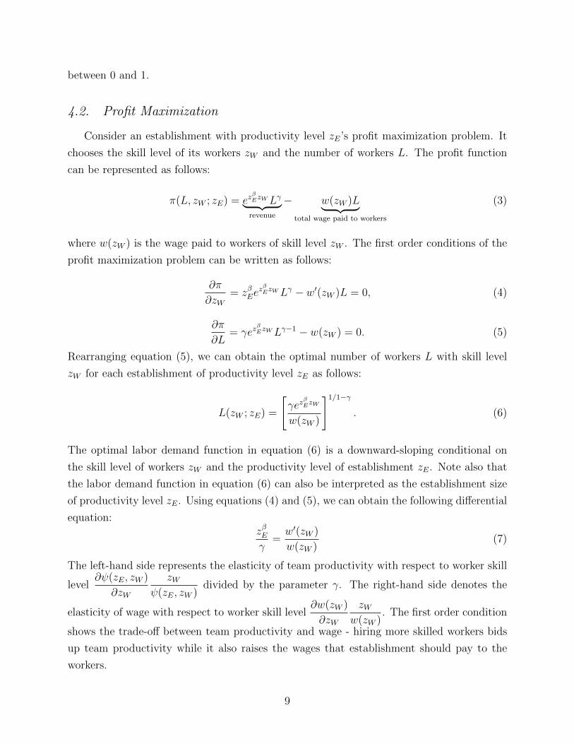
4.2. Profit Maximization

Consider an establishment with productivity level zE’s profit maximization problem. It

chooses the skill level of its workers zW and the number of workers L. The profit function

can be represented as follows:

π(L, zW ; zE) = ezβEzWLγ︸ ︷︷ ︸

revenue

− w(zW )L︸ ︷︷ ︸total wage paid to workers

(3)

where w(zW ) is the wage paid to workers of skill level zW . The first order conditions of the

profit maximization problem can be written as follows:

∂π

∂zW= zβEe

zβEzWLγ − w′(zW )L = 0, (4)

∂π

∂L= γez

βEzWLγ−1 − w(zW ) = 0. (5)

Rearranging equation (5), we can obtain the optimal number of workers L with skill level

zW for each establishment of productivity level zE as follows:

L(zW ; zE) =

[γez

βEzW

w(zW )

]1/1−γ

. (6)

The optimal labor demand function in equation (6) is a downward-sloping conditional on

the skill level of workers zW and the productivity level of establishment zE. Note also that

the labor demand function in equation (6) can also be interpreted as the establishment size

of productivity level zE. Using equations (4) and (5), we can obtain the following differential

equation:zβEγ

=w′(zW )

w(zW )(7)

The left-hand side represents the elasticity of team productivity with respect to worker skill

level∂ψ(zE, zW )

∂zW

zWψ(zE, zW )

divided by the parameter γ. The right-hand side denotes the

elasticity of wage with respect to worker skill level∂w(zW )

∂zW

zWw(zW )

. The first order condition

shows the trade-off between team productivity and wage - hiring more skilled workers bids

up team productivity while it also raises the wages that establishment should pay to the

workers.

9

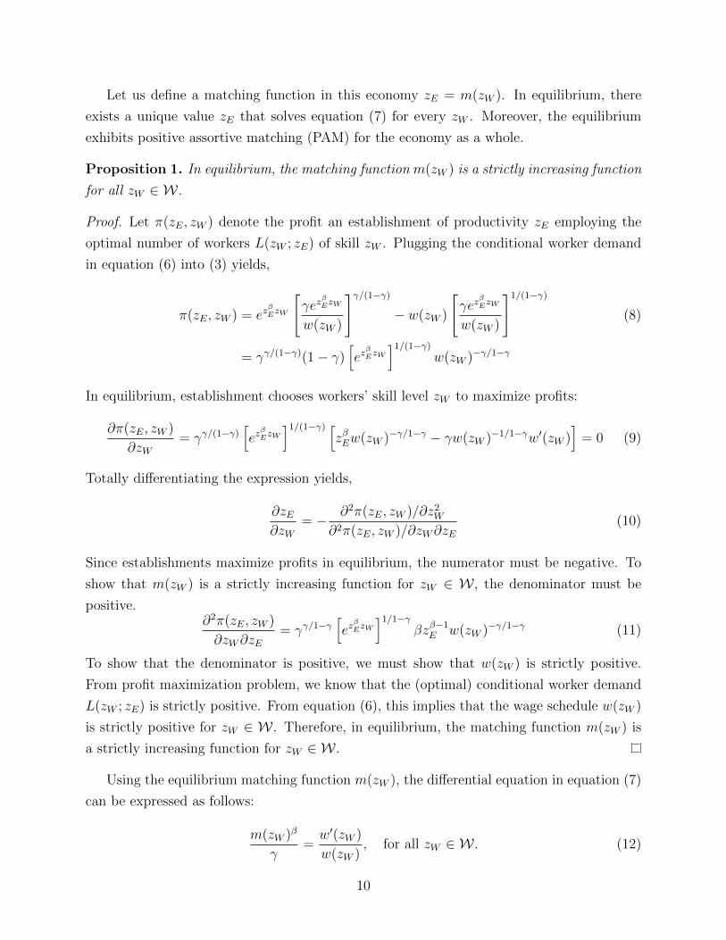
Let us define a matching function in this economy zE = m(zW ). In equilibrium, there

exists a unique value zE that solves equation (7) for every zW . Moreover, the equilibrium

exhibits positive assortive matching (PAM) for the economy as a whole.

Proposition 1. In equilibrium, the matching function m(zW ) is a strictly increasing function

for all zW ∈ W.

Proof. Let π(zE, zW ) denote the profit an establishment of productivity zE employing the

optimal number of workers L(zW ; zE) of skill zW . Plugging the conditional worker demand

in equation (6) into (3) yields,

π(zE, zW ) = ezβEzW

[γez

βEzW

w(zW )

]γ/(1−γ)

− w(zW )

[γez

βEzW

w(zW )

]1/(1−γ)

(8)

= γγ/(1−γ)(1− γ)[ezβEzW

]1/(1−γ)

w(zW )−γ/1−γ

In equilibrium, establishment chooses workers’ skill level zW to maximize profits:

∂π(zE, zW )

∂zW= γγ/(1−γ)

[ezβEzW

]1/(1−γ) [zβEw(zW )−γ/1−γ − γw(zW )−1/1−γw′(zW )

]= 0 (9)

Totally differentiating the expression yields,

∂zE∂zW

= − ∂2π(zE, zW )/∂z2W

∂2π(zE, zW )/∂zW∂zE(10)

Since establishments maximize profits in equilibrium, the numerator must be negative. To

show that m(zW ) is a strictly increasing function for zW ∈ W , the denominator must be

positive.∂2π(zE, zW )

∂zW∂zE= γγ/1−γ

[ezβEzW

]1/1−γβzβ−1

E w(zW )−γ/1−γ (11)

To show that the denominator is positive, we must show that w(zW ) is strictly positive.

From profit maximization problem, we know that the (optimal) conditional worker demand

L(zW ; zE) is strictly positive. From equation (6), this implies that the wage schedule w(zW )

is strictly positive for zW ∈ W . Therefore, in equilibrium, the matching function m(zW ) is

a strictly increasing function for zW ∈ W .

Using the equilibrium matching function m(zW ), the differential equation in equation (7)

can be expressed as follows:

m(zW )β

γ=w′(zW )

w(zW ), for all zW ∈ W . (12)

10

Solving the above differential equation and taking logs yields,

lnw(zW ) = ln w +

∫ zW

zW,min

m(z)β

γdz (13)

where w is the wage of the least skilled workers w = w(zW,min).

Proposition 2. The log wage schedule lnw(zL) is strictly increasing and convex in worker

skills1.

Proof. To show that the log wage schedule lnw(zW ) is strictly increasing, differentiating

lnw(zW ) with respect to zW results in

∂ lnw(zW )

∂zW=m(zW )β

γ> 0, for all zW ∈ W . (14)

Next, to prove that the log wage schedule lnw(zW ) is convex in skills, differentiating∂ lnw(zW )

∂zWwith respect to zW yields

∂2 lnw(zW )

∂z2W

= βm(zW )β−1m′(zW )

γ> 0, for all zW ∈ W . (15)

where the last inequality follows from positive assortative matching property of the matching

function m(zW ).

4.3. Factor Market Clearing

Consider a set of workers [zWa, zWb] and the set of establishments [m(zWa),m(zWb)] that

matched with these workers in the equilibrium. Factor market clearing condition can be

expressed as

E

∫ m(zWb)

m(zWa)

[γez

βm−1(z)

w(m−1(z))

]1/1−γ

φE(z)dz = W

∫ zWb

zWa

φW (z)dz (16)

where the left-hand side is the demand for workers by establishments with skill level between

m(zWa) and m(zWb) and the right-hand side is the supply of workers matched with those

establishments. After differentiating the factor market clearing condition with respect to

1Mincer (1958, 1974) models the logarithm of earnings as a function of years of education and experience,known as “The Mincer earnings function.” Following his insight, we focus on the log wage schedule ratherthan the wage schedule. Moreover, most empirical studies in this literature arena have analyzed the log wageschedule. Therefore, we use the log wage schedule as our benchmark analysis.

11

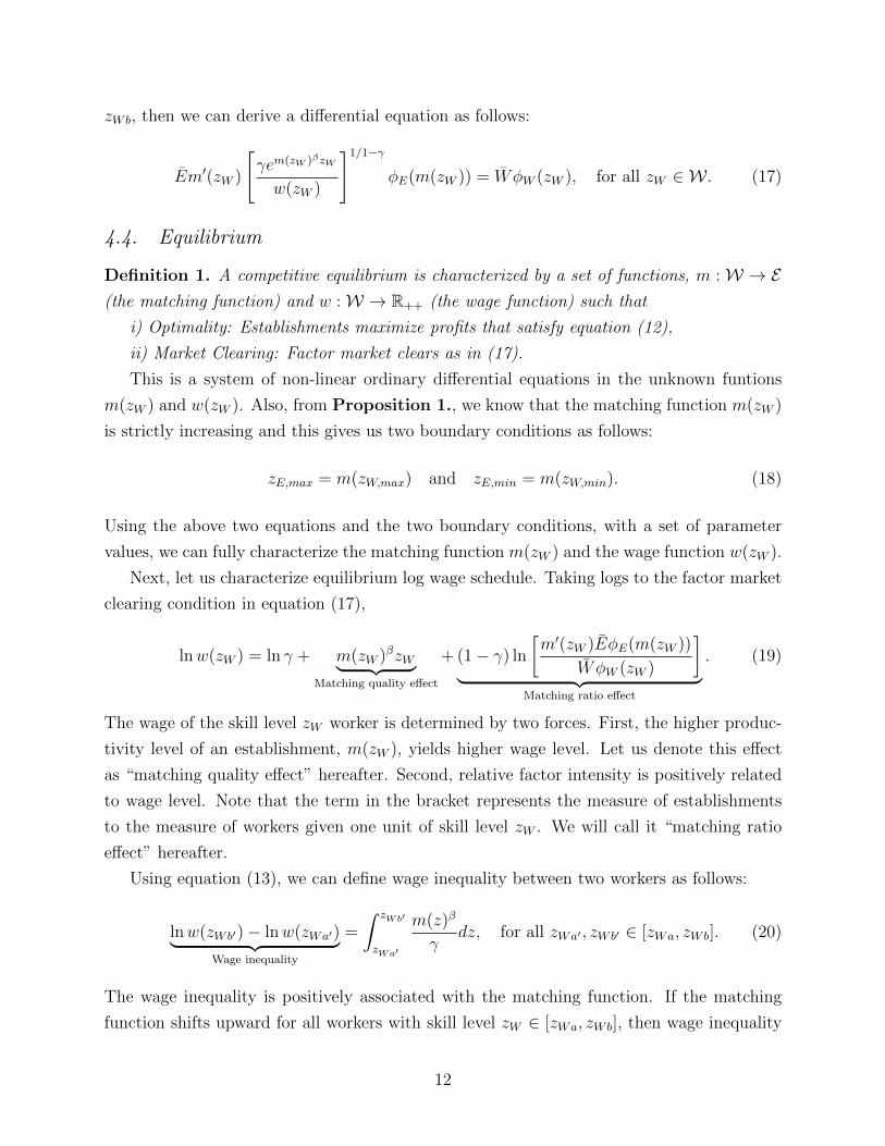
zWb, then we can derive a differential equation as follows:

Em′(zW )

[γem(zW )βzW

w(zW )

]1/1−γ

φE(m(zW )) = WφW (zW ), for all zW ∈ W . (17)

4.4. Equilibrium

Definition 1. A competitive equilibrium is characterized by a set of functions, m :W → E(the matching function) and w :W → R++ (the wage function) such that

i) Optimality: Establishments maximize profits that satisfy equation (12),

ii) Market Clearing: Factor market clears as in (17).

This is a system of non-linear ordinary differential equations in the unknown funtions

m(zW ) and w(zW ). Also, from Proposition 1., we know that the matching function m(zW )

is strictly increasing and this gives us two boundary conditions as follows:

zE,max = m(zW,max) and zE,min = m(zW,min). (18)

Using the above two equations and the two boundary conditions, with a set of parameter

values, we can fully characterize the matching function m(zW ) and the wage function w(zW ).

Next, let us characterize equilibrium log wage schedule. Taking logs to the factor market

clearing condition in equation (17),

lnw(zW ) = ln γ + m(zW )βzW︸ ︷︷ ︸Matching quality effect

+ (1− γ) ln

[m′(zW )EφE(m(zW ))

WφW (zW )

]︸ ︷︷ ︸

Matching ratio effect

. (19)

The wage of the skill level zW worker is determined by two forces. First, the higher produc-

tivity level of an establishment, m(zW ), yields higher wage level. Let us denote this effect

as “matching quality effect” hereafter. Second, relative factor intensity is positively related

to wage level. Note that the term in the bracket represents the measure of establishments

to the measure of workers given one unit of skill level zW . We will call it “matching ratio

effect” hereafter.

Using equation (13), we can define wage inequality between two workers as follows:

lnw(zWb′)− lnw(zWa′)︸ ︷︷ ︸Wage inequality

=

∫ zWb′

zWa′

m(z)β

γdz, for all zWa′ , zWb′ ∈ [zWa, zWb]. (20)

The wage inequality is positively associated with the matching function. If the matching

function shifts upward for all workers with skill level zW ∈ [zWa, zWb], then wage inequality

12

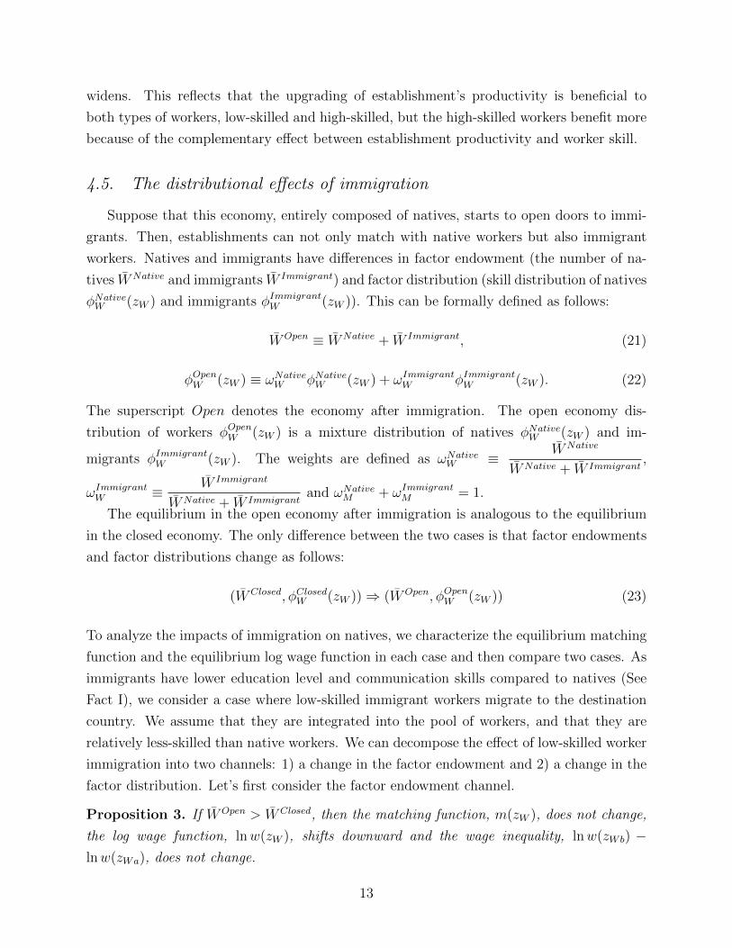
widens. This reflects that the upgrading of establishment’s productivity is beneficial to

both types of workers, low-skilled and high-skilled, but the high-skilled workers benefit more

because of the complementary effect between establishment productivity and worker skill.

4.5. The distributional effects of immigration

Suppose that this economy, entirely composed of natives, starts to open doors to immi-

grants. Then, establishments can not only match with native workers but also immigrant

workers. Natives and immigrants have differences in factor endowment (the number of na-

tives WNative and immigrants W Immigrant) and factor distribution (skill distribution of natives

φNativeW (zW ) and immigrants φImmigrantW (zW )). This can be formally defined as follows:

WOpen ≡ WNative + W Immigrant, (21)

φOpenW (zW ) ≡ ωNativeW φNativeW (zW ) + ωImmigrantW φImmigrantW (zW ). (22)

The superscript Open denotes the economy after immigration. The open economy dis-

tribution of workers φOpenW (zW ) is a mixture distribution of natives φNativeW (zW ) and im-

migrants φImmigrantW (zW ). The weights are defined as ωNativeW ≡ WNative

WNative + W Immigrant,

ωImmigrantW ≡ W Immigrant

WNative + W Immigrantand ωNativeM + ωImmigrantM = 1.

The equilibrium in the open economy after immigration is analogous to the equilibrium

in the closed economy. The only difference between the two cases is that factor endowments

and factor distributions change as follows:

(WClosed, φClosedW (zW ))⇒ (WOpen, φOpenW (zW )) (23)

To analyze the impacts of immigration on natives, we characterize the equilibrium matching

function and the equilibrium log wage function in each case and then compare two cases. As

immigrants have lower education level and communication skills compared to natives (See

Fact I), we consider a case where low-skilled immigrant workers migrate to the destination

country. We assume that they are integrated into the pool of workers, and that they are

relatively less-skilled than native workers. We can decompose the effect of low-skilled worker

immigration into two channels: 1) a change in the factor endowment and 2) a change in the

factor distribution. Let’s first consider the factor endowment channel.

Proposition 3. If WOpen > WClosed, then the matching function, m(zW ), does not change,

the log wage function, lnw(zW ), shifts downward and the wage inequality, lnw(zWb) −lnw(zWa), does not change.

13

Proof. Prove first that the matching function m(zW ) does not change. Rearranging equation

(17) yields,

lnw(zW )

1− γ=

ln γ

1− γ+ ln

[E

W

]+

lnα

1− γ+m(zW )βzW

1− γ+ lnφE(m(zW ))− lnφW (zW ) + lnm′(zW ).

(24)

By differentiating equation (24) with respect to zW and substituting (12) into the result, we

get the following second-order differential equation for the matching function m(zW ):

m′′(zW )

m′(zW )=m(zW )β

γ− βm(zW )β−1m′(zW )zW

1− γ+φ′W (zW )

φW (zW )− φ′E(m(zW ))m′(zW )

φE(m(zW )). (25)

The matching function does not depend on the factor endowments E and W , implying that

the matching function does not change. From equation (20), we know that wage inequality

do not change when the matching function stands still. From equation (24), one percent

increase in W decreases w(zW ) by 1− γ percent.

In this case, native establishments are now matched with more workers (both natives and

immigrants), thereby increasing the match ratio (the number of workers per establishment).

This will lead to more competition for native workers and the wages of native workers

decrease. However, in this case, the matching function m(zL) does not change so that there

is no inequality implications.

Next, let us analyze the effect of second channel in which the factor distribution changes

after immigration holding the factor endowment fixed. To analyze this case, we use the

concept of monotone likelihood ratio property as in Milgrom (1981) and Costinot and Vogel

(2010). The following definition is the monotone likelihood property and it extends the idea

of skill abundance in a two-factor model into a continuum of skill framework.

Definition 2. There are relatively more low-skilled workers after immigration ifφOpenW (z′W )

φOpenW (zW )≤

φClosedW (z′W )

φClosedW (zW )for all z′W ≥ zW .

Proposition 4. IfφOpenW (z′W )

φOpenW (zW )≤ φClosedW (z′W )

φClosedW (zW )for all z′W ≥ zW , then the matching function,

m(zW ), shifts upward and the wage inequality, lnw(zWb)− lnw(zWa), increases.

Proof. Suppose that there exists zW ∈ WOpen∩WClosed such that mOpen(zW ) < mClosed(zW ).

SinceφOpenW (z′W )

φOpenW (zW )≤ φClosedW (z′W )

φClosedW (zW ), we know that WOpen ∩ WClosed = [zClosedW,min, z

OpenW,max]. Posi-

tive assortative matching property of the matching function implies that mClosed(zClosedW,min) =

zM,min ≤ mOpen(zClosedW,min) and mOpen(zOpenW,max) = zM,max ≥ mClosed(zOpenW,max). So there must exist

14

zClosedW,min ≤ z1W ≤ z2

W ≤ zOpenW,max and zM,min ≤ z1M ≤ z2

M ≤ zM,max such that i) mClosed(z1W ) =

mOpen(z1W ) = z1

M and mClosed(z2W ) = mOpen(z2

W ) = z2M , ii) mClosed′(z1

W ) ≥ mOpen′(z1W )

and mOpen′(z2W ) ≥ mClosed′(z2

W ), and iii) mClosed(zW ) > mOpen(zW ) for all zW ∈ (z1W , z

2W ).

mClosed′(z1W ) ≥ mOpen′(z1

W ) and mOpen′(z2W ) ≥ mClosed′(z2

W ) implies that:

mClosed′(z1W )

mClosed′(z2W )≥ mOpen′(z1

W )

mOpen′(z2W )

(26)

Using equation (17), we can derive the following inequality:

φOpenW (z2W )

φOpenW (z1W )

[wOpen(z2

W )

wOpen(z1W )

]1/1−γ

≥ φClosedW (z2W )

φClosedW (z1W )

[wClosed(z2

W )

wClosed(z1W )

]1/1−γ

(27)

φOpenW (z2W )

φOpenW (z1W )≤ φClosedW (z2

W )

φClosedW (z1W )

requires that:

wOpen(z2W )

wOpen(z1W )≥ wClosed(z2

W )

wClosed(z1W )

(28)

However, this is a contradiction. Since mOpen(zW ) < mClosed(zW ), it must be that

wOpen(z2W )

wOpen(z1W )

<wClosed(z2

W )

wClosed(z1W )

(29)

Consequently, ifφOpenW (z′W )

φOpenW (zW )≤ φClosedW (z′W )

φClosedW (zW ), then mOpen(zW ) ≥ mClosed(zW ) for all WOpen ∩

WClosed.

Using equations (20) and (30), when the matching function m(zW ) shifts upward, it is

straightforward to see that the wage inequality, lnw(zWb)− lnw(zWa), increases.

Since immigrant workers are less-skilled than native workers, the lower part of the

worker’s skill distribution thickens. This induces native workers to be matched with higher

productive establishments, which is as an upward shift of the matching function m(zW ). The

match quality (the productivity level of matching counterparts) increases for native workers.

Due to the complementary effect, this raises native workers’ productivity and wages of native

workers increase conditional on the same matching ratio effect. By the log-supermodularity

of the production function, better workers benefit more from an increase in match quality

than other workers. Therefore, wage inequality within workers rises.

In sum, in the case of low-skilled worker immigrantion, the model predicts that immigrant

worker inflows would affect both the match ratio (the number of workers per establishment)

15

and the match quality (the skill level of matching counterparts). The match ratio effect would

lower the wage of native workers while the match quality effect would raise it. Through the

match quality channel, the inflow of low-skilled immigrants raises the wage inequality.

5. Numerical Simulations

This section reports simulation results of the equilibrium. In order to do so, we have

to set parameter values and functional forms defined in the equilibrium. First, using US

Census Bureau’s Statistics of U.S. Businesses in 2011, we can obtain both the number of

establishments and the number of workers in the U.S. (See Table 1). Second, we specify

functional forms of the distributions of establishment and worker φE(zE) and φW (zW ). As

our comparative static analysis relies on the definition of monotone likelihood ratio, we use

bounded pareto distributions with shape parameters ξE and ξW among distributions that

satifying this property:

φE(zE) =ξE(zE,min)ξE(zE)−ξE−1

1−(zE,minzE,max

)ξE and φW (zW ) =ξW (zW,min)ξW (zW )−ξW−1

1−(zW,minzW,max

)ξW . (30)

We choose a set of establishment productivity level E , a set of worker skill level W , and

shape parameters ξE and ξW as in Table 1. Third, we set the parameter β to be 1.25. In

Kremer and Maskin (1996, 2006)’s production function z2EzW , establishment productivity is

raised to number 2, however, our team productivity is ezβEzW . In our case, β = 1.25, team

productivity ranges from 2.72 (the lowest) to 116.38 (the highest). Lastly, following Atkeson

and Kehoe (2005), the share paid to workers within establishment is set to be 65 percent.

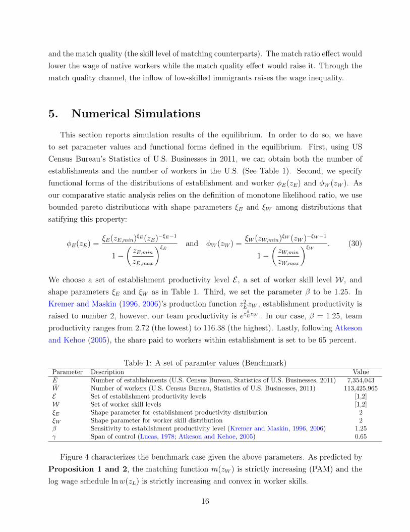
Table 1: A set of paramter values (Benchmark)Parameter Description ValueE Number of establishments (U.S. Census Bureau, Statistics of U.S. Businesses, 2011) 7,354,043W Number of workers (U.S. Census Bureau, Statistics of U.S. Businesses, 2011) 113,425,965E Set of establishment productivity levels [1,2]W Set of worker skill levels [1,2]ξE Shape parameter for establishment productivity distribution 2ξW Shape parameter for worker skill distribution 2β Sensitivity to establishment productivity level (Kremer and Maskin, 1996, 2006) 1.25γ Span of control (Lucas, 1978; Atkeson and Kehoe, 2005) 0.65

Figure 4 characterizes the benchmark case given the above parameters. As predicted by

Proposition 1 and 2, the matching function m(zW ) is strictly increasing (PAM) and the

log wage schedule lnw(zL) is strictly increasing and convex in worker skills.

16

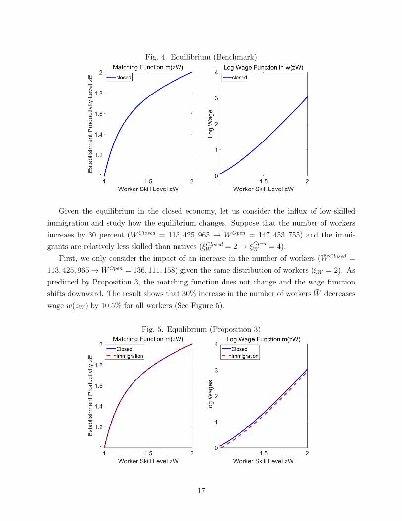
Fig. 4. Equilibrium (Benchmark)

Given the equilibrium in the closed economy, let us consider the influx of low-skilled

immigration and study how the equilibrium changes. Suppose that the number of workers

increaes by 30 percent (WClosed = 113, 425, 965 → WOpen = 147, 453, 755) and the immi-

grants are relatively less skilled than natives (ξClosedW = 2→ ξOpenW = 4).

First, we only consider the impact of an increase in the number of workers (WClosed =

113, 425, 965→ WOpen = 136, 111, 158) given the same distribution of workers (ξW = 2). As

predicted by Proposition 3, the matching function does not change and the wage function

shifts downward. The result shows that 30% increase in the number of workers W decreases

wage w(zW ) by 10.5% for all workers (See Figure 5).

Fig. 5. Equilibrium (Proposition 3)

17

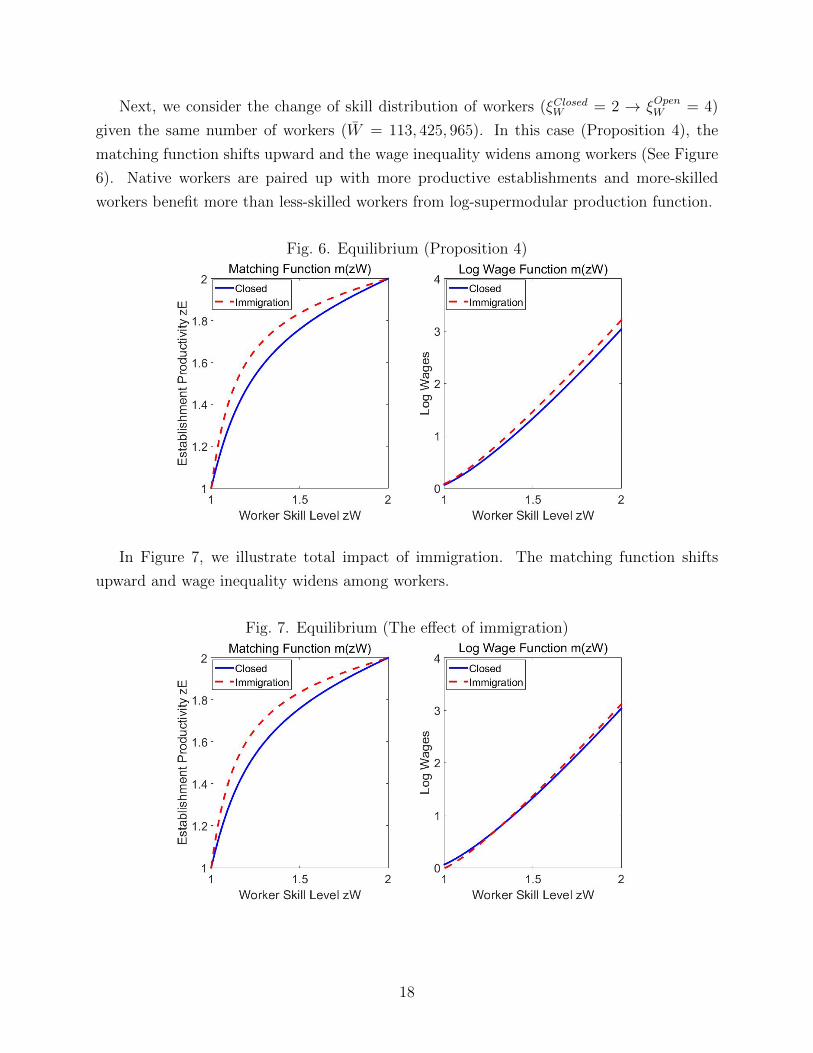
Next, we consider the change of skill distribution of workers (ξClosedW = 2 → ξOpenW = 4)

given the same number of workers (W = 113, 425, 965). In this case (Proposition 4), the

matching function shifts upward and the wage inequality widens among workers (See Figure

6). Native workers are paired up with more productive establishments and more-skilled

workers benefit more than less-skilled workers from log-supermodular production function.

Fig. 6. Equilibrium (Proposition 4)

In Figure 7, we illustrate total impact of immigration. The matching function shifts

upward and wage inequality widens among workers.

Fig. 7. Equilibrium (The effect of immigration)

18

6. Empirical Analysis

In this section, we analyze whether our theoretical model can explain the effect of influx

of immigrants on natives in the U.S. from 1980 through 2010. First, we give an overview

of our dataset and construct key variables. Then we empirically show that the immigrant

inflow increases the inequality among natives, consistent with our theory, and show that the

worker-firm matching channel exists. Lastly, we further analyze the mechanism to show that

the data fits the details of the theoretical model.

6.1. Data and variables

6.1.1. Data overview

Our primary datasets are 5% 1980, 1990, 2000 U.S. Census and 2009-2011 3-year IPUMS

American Community Survey for 2010. Samples are restricted to all individuals in age 18 to

64. ‘Immigrants’ refer to individuals who were born in a foreign country, and ‘natives’ refer

to those who were born in the U.S.2 We use commuting zones as geographical unit following

Autor and Dorn (2013) and Basso and Peri (2015) (section 6.1.2). An instrumental variable

for share of immigrants in each year and commuting zone is estimated by shift-share method

based on the foreign born population in the 1% 1950 U.S. Census (section 6.1.3).

Hourly wages are calculated by dividing the wage and salary income by weeks worked

and usual hours worked per week. Hourly wages in the lowest and highest 1% of the distri-

bution and those of less than one dollar are dropped. Managers and workers are grouped

by the occupation as in [Table 2]. Industries are grouped as [Table 3]. There are 28,434,461

observations, including 25,213,125 natives and 3,221,336 immigrants.

6.1.2. Commuting zone

We use commuting zones as primary geographical unit following Autor and Dorn (2013)

and Basso and Peri (2015). States are too large to represent local labor markets, and counties

are too small and often do not overlap with labor market regions. Metropolitan areas include

regions around urban areas, and have limitation representing rural areas. Commuting Zones

are developed by Tolbert and Sizer (1996) to approximate local labor markets and they

can be consistently constructed over full period of our analysis. Application of commuting

zones require some complexity, however, since commuting zones are not directly provided by

Census data and since some geographical units are matched to multiple commuting zones.

2U.S. territories are excluded.

19

The U.S. Census and American Community Survey files provide geographical units that

are smaller than states –State Economic Areas (1950), Country Groups (1980), and Public

Use Micro Area (PUMA, 1990, 2000, 2009-2011).3 These geographical units are mapped to

commuting zones using the mapping file (http://ddorn.net/). While many units fall into a

single CZ, some geographical units are matched to several CZs with each probability. For

example, 20% of workers in a PUMA commute to the first CZ and 80% to the second CZ.

Each observations in that PUMA is now split into two CZs with probability .2 and .8, and

personal weights are also split by .2 and .8 (Autor and Dorn, 2013).

6.1.3. Share of immigrants

The number of immigrants in each commuting zone is endogenously determined by pull

factors of each region, such as labor market condition. To remove the endogeneity, we

construct an instrumental variable for share of immigrants (ImmigShareRAWg,t ) by shift-share

method based on the foreign born population in 1950 US Census.

P opg,o,t = Popg,o,1950 ∗PopUS,o,tPopUS,o,1950

(o = US and other origin countries)

ImmigShareIVg,t =

∑o 6=US P opg,o,t∑o P opg,o,t

(31)

We group origin countries into 16 origin regions.4 For each origin region o, immigrant

population in 1950 in commuting zone g (Popg,o,1950) is increased by the national increase

rate between 1950 and year t (PopUS,o,t

PopUS,o,1950). Stock of native population in each commuting

zone and year is estimated similarly and noted as o = US. We calculate the stock of all

immigrants in each commuting zone aggregating the number of immigrants over all origin

regions, excluding the U.S. Share of immigrants in commuting zone g and year t is calculated

by the stock of all immigrants (∑

o 6=US P opg,o,t) divided by the sum of both immigrants and

natives (∑

o P opg,o,t).

First stage regression verifies that ImmigShareIVg,t is a strong instrumental variable for

ImmigShareRAWg,t . ...

3PUMA in 1960 Census was recently released, but we have not used the data yet.4Sixteen origin regions are United States, Other North America, Central America and Caribbean,

South America, Northern Europe, United Kingdom and Ireland, Western Europe, Southern Europe, Cen-tral/Eastern Europe, Russian Empire, East Asia, Southeast Asia, India/Southwest Asia, Middle East/AsiaMinor, Africa, and Oceania.

20

6.1.4. Worker quality and firm quality

To test the worker-firm matching, we need to define the unit of firm and the measure of

firm quality. Previous papers investigating worker-firm matching (or worker-establishment

matching, worker-job matching) used datasets that could identify the actual establishment

and that could track workers moving across establishments through the years (REF). How-

ever, our dataset does not include establishment or firm information, and we cannot track

workers since it is cross-sectional data. Instead we define commuting zone - industry as a

proxy for “firm”. Industry is categorized into 00 groups (Table 3) and each firm (commut-

ing zone - industry - year) hires 00 individuals on average. We use individual observable

characteristics to isolate firm effects, and use distribution of workers to estimate the move

of workers across firms.

Following REF, Firm quality, or firm productivity, is estimated as firm fixed effects from

log hourly wage of each individual. We control for individual characteristics, which include

sex, age, age square, level of education dummies (less than high school, high school, some

college, more than college), immigrant dummy, manager dummy, and year fixed effects.

Higher firm quality represents that the firm has higher productivity and it can pay workers

higher wages since it shares some of the profit with workers. [Table 4] summarizes the effect

of observable characteristics on log wage, and [Figure 9] shows the distribution of estimated

firm quality in a sample commuting zone-year.

Ln(HourlyWage)i,g,j,t = α0 + α1Sexi + α2Agei + α3Age2i + α4Edui + α5Immigranti

+ α6Manageri + α7FirmQualityg,j + φt + εi,g,j,t (32)

Worker quality is assumed as either level of education, or imputed wage from observable

characteristics with the firm quality set at the mean. [Figure 10] shows the distribution of

worker quality in both measures.

6.2. Check assumptions

Using the U.S. Census 2010 dataset, we present some features of the U.S. labor market,

which validates the model’s equilibrium features.

6.2.1. Positive assortative matching

In the theoretical model, we assumed that better workers are matched with firms with

higher productivity (positive assortative matching). From the measure drawn from 6.1.4,

21

we draw [Figure 11] which shows the positive relation with worker quality and firm quality.

Figure (a) and figure (b) shows level of education and imputed wage of workers, respectively.

6.2.2. Log Supermodularity

In the theoretical model, we assumed that better workers benefit more from being

matched with better firms (log supermodularity, or complementarity with workers and firms).

To verify the assumption, we test whether the interaction between worker quality (level of

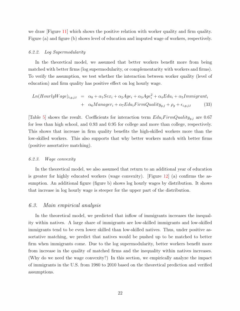
education) and firm quality has positive effect on log hourly wage.

Ln(HourlyWage)i,g,j,t = α0 + α1Sexi + α2Agei + α3Age2i + α4Edui + α5Immigranti

+ α6Manageri + α7EduiFirmQualityg,j + ρg + εi,g,j,t (33)

[Table 5] shows the result. Coefficients for interaction term EduiFirmQualityg,j are 0.67

for less than high school, and 0.93 and 0.95 for college and more than college, respectively.

This shows that increase in firm quality benefits the high-skilled workers more than the

low-skilled workers. This also supports that why better workers match with better firms

(positive assortative matching).

6.2.3. Wage convexity

In the theoretical model, we also assumed that return to an additional year of education

is greater for highly educated workers (wage convexity). [Figure 12] (a) confirms the as-

sumption. An additional figure (figure b) shows log hourly wages by distribution. It shows

that increase in log hourly wage is steeper for the upper part of the distribution.

6.3. Main empirical analysis

In the theoretical model, we predicted that inflow of immigrants increases the inequal-

ity within natives. A large share of immigrants are low-skilled immigrants and low-skilled

immigrants tend to be even lower skilled than low-skilled natives. Thus, under positive as-

sortative matching, we predict that natives would be pushed up to be matched to better

firm when immigrants come. Due to the log supermodularity, better workers benefit more

from increase in the quality of matched firms and the inequality within natives increases.

(Why do we need the wage convexity?) In this section, we empirically analyze the impact

of immigrants in the U.S. from 1980 to 2010 based on the theoretical prediction and verified

assumptions.

22

6.3.1. The effect of immigrant inflow on inequality

First, we test whether inflow of immigrants increases the inequality within natives.

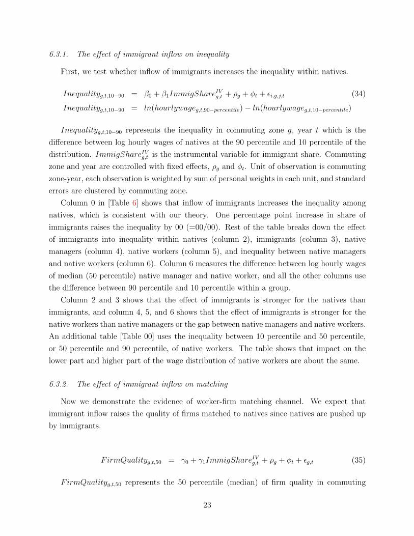
Inequalityg,t,10−90 = β0 + β1ImmigShareIVg,t + ρg + φt + εi,g,j,t (34)

Inequalityg,t,10−90 = ln(hourlywageg,t,90−percentile)− ln(hourlywageg,t,10−percentile)

Inequalityg,t,10−90 represents the inequality in commuting zone g, year t which is the

difference between log hourly wages of natives at the 90 percentile and 10 percentile of the

distribution. ImmigShareIVg,t is the instrumental variable for immigrant share. Commuting

zone and year are controlled with fixed effects, ρg and φt. Unit of observation is commuting

zone-year, each observation is weighted by sum of personal weights in each unit, and standard

errors are clustered by commuting zone.

Column 0 in [Table 6] shows that inflow of immigrants increases the inequality among

natives, which is consistent with our theory. One percentage point increase in share of

immigrants raises the inequality by 00 (=00/00). Rest of the table breaks down the effect

of immigrants into inequality within natives (column 2), immigrants (column 3), native

managers (column 4), native workers (column 5), and inequality between native managers

and native workers (column 6). Column 6 measures the difference between log hourly wages

of median (50 percentile) native manager and native worker, and all the other columns use

the difference between 90 percentile and 10 percentile within a group.

Column 2 and 3 shows that the effect of immigrants is stronger for the natives than

immigrants, and column 4, 5, and 6 shows that the effect of immigrants is stronger for the

native workers than native managers or the gap between native managers and native workers.

An additional table [Table 00] uses the inequality between 10 percentile and 50 percentile,

or 50 percentile and 90 percentile, of native workers. The table shows that impact on the

lower part and higher part of the wage distribution of native workers are about the same.

6.3.2. The effect of immigrant inflow on matching

Now we demonstrate the evidence of worker-firm matching channel. We expect that

immigrant inflow raises the quality of firms matched to natives since natives are pushed up

by immigrants.

FirmQualityg,t,50 = γ0 + γ1ImmigShareIVg,t + ρg + φt + εg,t (35)

FirmQualityg,t,50 represents the 50 percentile (median) of firm quality in commuting

23

zone g and year t where firm quality matched to each native constructs the distribution.

ImmigShareIVg,t is the instrumental variable for immigrant share. Commuting zone and year

are controlled with fixed effects, ρg and φt. Unit of observation is commuting zone-year, and

each observation is weighted by sum of personal weights in each unit.

We expect γ1 to be positive and [Table 7] column 3 shows that the result is consistent

with our prediction. One percentage point increase in immigrant share raises the median

firm quality by 00 (=00/00). We later analyze this with different percentiles of firm quality

to see the impact on natives other than the median.

6.3.3. Contribution of matching channel on inequality

Did the change in inequality (section 6.3.1) occur through the worker-firm matching

channel (section 6.3.2)? We decompose the impact of immigrants on inequality into a portion

due to commuting zone and year fixed effects, a portion through the matching channel, and

a portion that is unrelated to the matching channel.

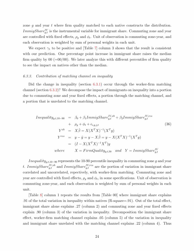
Inequalityg,t,10−90 = β0 + β1ImmigShareIV,xbg,t + β2ImmigShare

IV,resg,t

+ ρg + φt + εi,g,j,t (36)

Y xb = Xβ = X(XTX)−1(XTy)

Y res = y − y = y −Xβ = y −X(XTX)−1(XTy)

= (I −X(XTX)−1XT )y

where X = FirmQualityg,t,50 and Y = ImmigShareIVg,t

Inequalityg,t,10−90 represents the 10-90 percentile inequality in commuting zone g and year

t. ImmigShareIV,xbg,t and ImmigShareIV,resg,t are the portion of variation in immigrant share

correlated and uncorrelated, repectively, with worker-firm matching. Commuting zone and

year are controlled with fixed effects, ρg and φt, in some specifications. Unit of observation is

commuting zone-year, and each observation is weighted by sum of personal weights in each

unit.

[Table 8] column 1 repeats the results from [Table 00] where immigrant share explains

.91 of the total variation in inequality within natives (R-square=.91). Out of the total effect,

immigrant share alone explains .27 (column 2) and commuting zone and year fixed effects

explain .90 (column 3) of the variation in inequality. Decomposition the immigrant share

effect, worker-firm matching channel explains .05 (column 5) of the variation in inequality

and immigrant share unrelated with the matching channel explains .22 (column 4). Thus

24

the matching channel explains around 00 (=.05/.27) of the immigrant effect on inequality.

An additional table [Table 00] also shows similar results. Worker-firm matching channel

together with commuting zone and year fixed effects explains .90 of the variation in inequality

(column 2), and matching channel alone explains .05 (column 3).

6.4. Channels

In previous section, we showed that when immigrants – who tend to have lower-skilled

than natives – come, they are likely to change the worker-firm matching of natives, and this

increases the inequality within natives due to the log supermodularity. In this section, we

investigate further into the channels of how immigrants affect the inequality.

6.4.1. Linear and convex effect

Section 6.3.2 shows that immigrants raises the match quality – quality of the matched

firm – for median native. How about the natives at the lower and higher part of the wage

distribution? Does inequality increase because better workers experience greater increase in

the match quality? Or is it because better workers benefit more from the same increase in

the match quality – due to log supermodularity – even they experience the same amount of

increase in the match quality?

First, we test whether natives at the higher part of the wage distribution experience

greater increase in the match quality. We repeat (eq 35) replacing the 50-percentile with

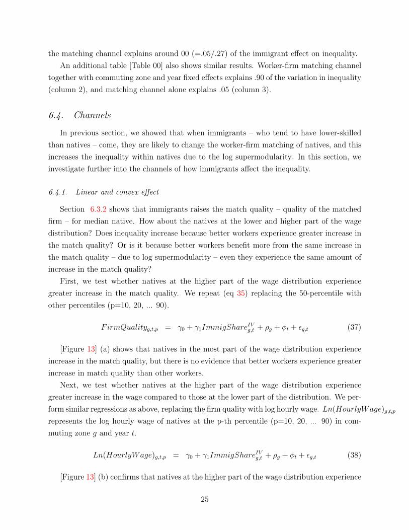
other percentiles (p=10, 20, ... 90).

FirmQualityg,t,p = γ0 + γ1ImmigShareIVg,t + ρg + φt + εg,t (37)

[Figure 13] (a) shows that natives in the most part of the wage distribution experience

increase in the match quality, but there is no evidence that better workers experience greater

increase in match quality than other workers.

Next, we test whether natives at the higher part of the wage distribution experience

greater increase in the wage compared to those at the lower part of the distribution. We per-

form similar regressions as above, replacing the firm quality with log hourly wage. Ln(HourlyWage)g,t,p

represents the log hourly wage of natives at the p-th percentile (p=10, 20, ... 90) in com-

muting zone g and year t.

Ln(HourlyWage)g,t,p = γ0 + γ1ImmigShareIVg,t + ρg + φt + εg,t (38)

[Figure 13] (b) confirms that natives at the higher part of the wage distribution experience

25

greater increase in wage compared to the native at the lower part. Especially, natives at

the 10th- and 20th-percentile show significant decrease in wage with the immigrant inflow.

Together with the log supermodularity and wage convexity shown in section 6.2.2 and 6.2.3,

this supports that inequality increase due to the nonlinear attribute.

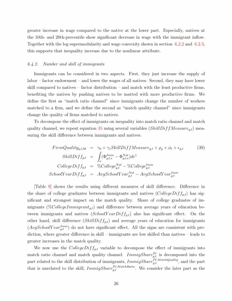
6.4.2. Number and skill of immigrants

Immigrants can be considered in two aspects. First, they just increase the supply of

labor – factor endowment – and lower the wages of all natives. Second, they may have lower

skill compared to natives – factor distribution – and match with the least productive firms,

benefiting the natives by pushing natives to be matted with more productive firms. We

define the first as “match ratio channel” since immigrants change the number of workers

matched to a firm, and we define the second as “match quality channel” since immigrants

change the quality of firms matched to natives.

To decompose the effect of immigrants on inequality into match ratio channel and match

quality channel, we repeat equation 35 using several variables (SkillDiffMeasureg,t) mea-

suring the skill difference between immigrants and natives.

FirmQualityg,t,50 = γ0 + γ1SkillDiffMeasureg,t + ρg + φt + εg,t (39)

SkillDiffg,t =

∫e

(ΦImmg,t,e − ΦNat

g,t,e)de5

CollegeDiffg,t = %CollegeNatg,t −%CollegeImmg,t

SchoolY earDiffg,t = AvgSchoolY earNatg,t − AvgSchoolY earImmg,t

[Table 9] shows the results using different measures of skill difference. Difference in

the share of college graduates between immigrants and natives (CollegeDiffg,t) has sig-

nificant and strongest impact on the match quality. Share of college graduates of im-

migrants (%CollegeImmigrantg,t) and difference between average years of education be-

tween immigrants and natives (SchoolY earDiffg,t) also has significant effect. On the

other hand, skill difference (SkillDiffg,t) and average years of education for immigrants

(AvgSchoolY earImmg,t ) do not have significant effect. All the signs are consistent with pre-

diction, where greater difference in skill – immigrants are low skilled than natives – leads to

greater increases in the match quality.

We now use the CollegeDiffg,t variable to decompose the effect of immigrants into

match ratio channel and match quality channel. ImmigShareIVg,t is decomposed into the

part related to the skill distribution of immigrants, ImmigShareIV,MatchQualityg,t , and the part

that is unrelated to the skill, ImmigShareIV,MatchRatiog,t . We consider the later part as the

26

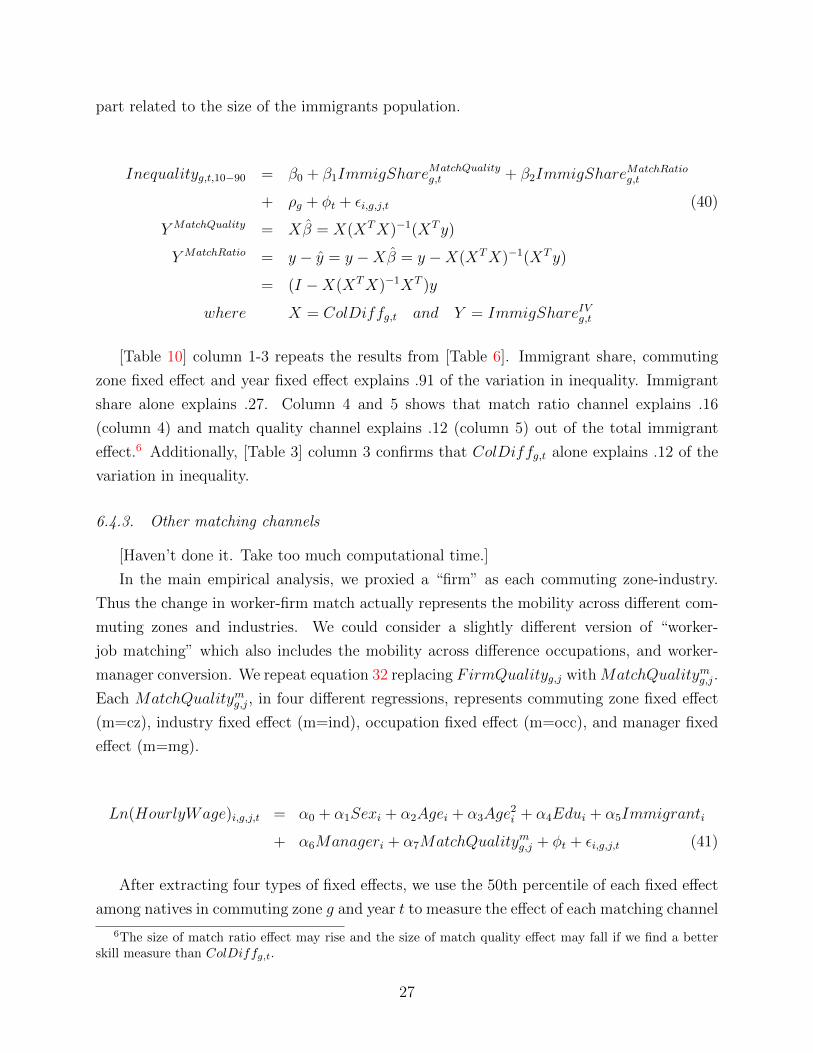
part related to the size of the immigrants population.

Inequalityg,t,10−90 = β0 + β1ImmigShareMatchQualityg,t + β2ImmigShare

MatchRatiog,t

+ ρg + φt + εi,g,j,t (40)

Y MatchQuality = Xβ = X(XTX)−1(XTy)

Y MatchRatio = y − y = y −Xβ = y −X(XTX)−1(XTy)

= (I −X(XTX)−1XT )y

where X = ColDiffg,t and Y = ImmigShareIVg,t

[Table 10] column 1-3 repeats the results from [Table 6]. Immigrant share, commuting

zone fixed effect and year fixed effect explains .91 of the variation in inequality. Immigrant

share alone explains .27. Column 4 and 5 shows that match ratio channel explains .16

(column 4) and match quality channel explains .12 (column 5) out of the total immigrant

effect.6 Additionally, [Table 3] column 3 confirms that ColDiffg,t alone explains .12 of the

variation in inequality.

6.4.3. Other matching channels

[Haven’t done it. Take too much computational time.]

In the main empirical analysis, we proxied a “firm” as each commuting zone-industry.

Thus the change in worker-firm match actually represents the mobility across different com-

muting zones and industries. We could consider a slightly different version of “worker-

job matching” which also includes the mobility across difference occupations, and worker-

manager conversion. We repeat equation 32 replacing FirmQualityg,j withMatchQualitymg,j.

Each MatchQualitymg,j, in four different regressions, represents commuting zone fixed effect

(m=cz), industry fixed effect (m=ind), occupation fixed effect (m=occ), and manager fixed

effect (m=mg).

Ln(HourlyWage)i,g,j,t = α0 + α1Sexi + α2Agei + α3Age2i + α4Edui + α5Immigranti

+ α6Manageri + α7MatchQualitymg,j + φt + εi,g,j,t (41)

After extracting four types of fixed effects, we use the 50th percentile of each fixed effect

among natives in commuting zone g and year t to measure the effect of each matching channel

6The size of match ratio effect may rise and the size of match quality effect may fall if we find a betterskill measure than ColDiffg,t.

27

on inequality.

Inequalityg,t,10−90 = β0 + β1MatchQualityczg,j,50 + β2MatchQualityindg,j,50

+ β3MatchQualityoccg,j,50 + β4MatchQualitymgg,j,50 + ρg + φt + εi,g,j,t(42)

7. Conclusion

This paper introduces a novel channel - a matching between workers and establishments

- to the literature on the effect of immigrants on wages and inequality of natives in the

destination country. Based on a worker-establishment matching framework adopted from

the assignment model in trade literature, we expect that the influx of immigrants affects

natives through two channels - match ratio and match quality. Since heterogeneous workers

and establishments are differently affected by immigrants, change in inequality within native

workers and native establishments depends on the skill distribution of incoming immigrants.

Data show that low-skilled immigrants in the U.S. tend to have lower skills than native

workers. Using the U.S. data from 1980 to 2010 and exploiting the variation in immigrant

share across states and years, we investigate whether our theoretical model can explain the

change in the inequality of natives from the inflow of low-skilled immigration. We also track

through the channels to identify whether the immigrant inflow operated through the match

quality channel. Results show that the change in match quality is consistent with our model’s

prediction where native workers are paired up with higher skilled establishments from the

low-skilled immigration. Moreover, immigrant inflows tend to push some native workers to

switch to a establishment. Inequality within native workers, which is our primary interest,

increases by low-skilled immigrants as predicted in the model.

We further pursue the following research agendas in the future. First, we plan to enhance

the theoretical model by relaxing the assumption of the exogeneity of factor endowments

of establishments and workers. Agents can then endogenously choose their tasks, i.e. a

establishment and a worker, depending on the local labor market conditions. Second, we

seek to implement empirical analysis using better dataset, such as firm-level dataset, to test

our model. As we do not have firm-level dataset our empirical apporoach is an approximation.

If we have firm-level dataset, we can figure out more detailed determinants of the matching

between workers and establishments. Lastly, we seek to include measures of match ratio and

probability of being a establishment in the inequality regression, thereby decomposing the

effect of each channel and isolating the effect of match quality channel.

28

References

Acemoglu, D. and D. Autor (2011): “Skills, tasks and technologies: Implications foremployment and earnings,” Handbook of labor economics, 4, 1043–1171.

Acemoglu, D., D. Dorn, G. H. Hanson, B. Price, et al. (2014): “Import compe-tition and the Great US Employment Sag of the 2000s,” Tech. rep., National Bureau ofEconomic Research.

Aitken, B., A. Harrison, and R. E. Lipsey (1996): “Wages and foreign ownership Acomparative study of Mexico, Venezuela, and the United States,” Journal of internationalEconomics, 40, 345–371.

Antras, P., L. Garicano, and E. Rossi-Hansberg (2006): “Offshoring in a KnowledgeEconomy,” The Quarterly Journal of Economics, 121, 31–77.

Atkeson, A. and P. J. Kehoe (2005): “Modeling and measuring organization capital,”Journal of Political Economy, 113, 1026–1053.

Autor, D. H. and D. Dorn (2013): “The Growth of Low-Skill Service Jobs and thePolarization of the US Labor Market,” American Economic Review, 103, 1553–97.

Basso, G. and G. Peri (2015): “The Association between Immigration and Labor MarketOutcomes in the United States,” .

Bloom, N., M. Draca, and J. Van Reenen (2011): “Trade induced technical change?The impact of Chinese imports on innovation, IT and productivity,” Tech. rep., NationalBureau of Economic Research.

Bloom, N., B. Eifert, A. Mahajan, D. McKenzie, and J. Roberts (2013): “DoesManagement Matter? Evidence from India,” The Quarterly Journal of Economics, 128,1–51.

Borjas, G. J. (2003): “The Labor Demand Curve Is Downward Sloping: Reexaminingthe Impact of Immigration on the Labor Market,” The Quarterly Journal of Economics,1335–1374.

Card, D. (1990): “The impact of the Mariel boatlift on the Miami labor market,” Industrial& Labor Relations Review, 43, 245–257.

——— (2009): “Immigration and Inequality,” The American economic review, 99, 1–21.

Choi, J. (2016): “Offshoring and inequality: A matching and sorting model of offshoring,”.

Costinot, A. and J. Vogel (2010): “Matching and Inequality in the World Economy,”Journal of Political Economy, 118, 747–786.

29

Earle, J. S., A. Telegdy, and G. Antal (2013): “FDI and Wages: Evidence fromFirm-Level and Linked Employer-Employee Data in Hungary, 1986-2008,” GMU Schoolof Public Policy Research Paper.

Ebenstein, A., A. Harrison, M. McMillan, and S. Phillips (2014): “Estimatingthe impact of trade and offshoring on American workers using the current populationsurveys,” Review of Economics and Statistics, 96, 581–595.

Elsby, M. W., B. Hobijn, and A. Sahin (2010): “The labor market in the GreatRecession,” Tech. rep., National Bureau of Economic Research.

Feenstra, R. C. and G. H. Hanson (1996): “Foreign Investment, Outsourcing, and Rel-ative Wages,” The political economy of trade policy: papers in honor of Jagdish Bhagwati,89–127.

——— (1997): “Foreign direct investment and relative wages: Evidence from Mexico’smaquiladoras,” Journal of international economics, 42, 371–393.

——— (1999): “The impact of outsourcing and high-technology capital on wages: estimatesfor the United States, 1979-1990,” Quarterly Journal of Economics, 907–940.

Feenstra, R. C. and J. B. Jensen (2012): “Evaluating Estimates of Materials Offshoringfrom US Manufacturing,” Tech. rep., National Bureau of Economic Research.

Freeman, R. B. and R. Oostendorp (2000): “Wages around the world: pay acrossoccupations and countries,” Tech. rep., National Bureau of Economic Research.

Fukase, E. (2014): “Foreign wage premium, gender and education: Insights from Vietnamhousehold surveys,” The World Economy, 37, 834–855.

Gandal, N., G. H. Hanson, and M. J. Slaughter (2004): “Technology, trade, andadjustment to immigration in Israel,” European Economic Review, 48, 403–428.

Garicano, L. (2000): “Hierarchies and the Organization of Knowledge in Production,”Journal of political economy, 108, 874–904.

Grossman, G. M., E. Helpman, and P. Kircher (2013): “Matching and sorting in aglobal economy,” Tech. rep., National Bureau of Economic Research.

Grossman, G. M. and G. Maggi (2000): “Diversity and Trade,” American EconomicReview, 90, 1255–1275.

Grossman, G. M. and E. Rossi-Hansberg (2008): “Trading Tasks: A Simple Theoryof Offshoring,” The American Economic Review, 1978–1997.

Hijzen, A., P. S. Martins, T. Schank, and R. Upward (2013): “Foreign-owned firmsaround the world: A comparative analysis of wages and employment at the micro-level,”European Economic Review, 60, 170–188.

30

Hunt, J. and M. Gauthier-Loiselle (2010): “How Much Does Immigration BoostInnovation?” American Economic Journal: Macroeconomics, 31–56.

Kremer, M. (1993): “The O-ring theory of economic development,” The Quarterly Journalof Economics, 551–575.

Kremer, M. and E. Maskin (1996): “Wage inequality and segregation by skill,” Tech.rep., National Bureau of Economic Research.

——— (2006): “Globalization and inequality,” .

Lemieux, T. (2006): “Postsecondary Education and Increasing Wage Inequality,” TheAmerican Economic Review, 195–199.

——— (2008): “The changing nature of wage inequality,” Journal of Population Economics,21, 21–48.

Lipsey, R. E. and F. Sjoholm (2004): “Foreign direct investment, education and wagesin Indonesian manufacturing,” Journal of Development Economics, 73, 415–422.

Lucas, R. E. (1978): “On the size distribution of business firms,” The Bell Journal ofEconomics, 508–523.

Milgrom, P. R. (1981): “Good news and bad news: Representation theorems and appli-cations,” The Bell Journal of Economics, 380–391.

Mincer, J. (1958): “Investment in human capital and personal income distribution,” Jour-nal of Political Economy, 281–302.

Mincer, J. A. (1974): “Schooling, Experience, and Earnings,” .

Monte, F. (2011): “Skill bias, trade, and wage dispersion,” Journal of International Eco-nomics, 83, 202–218.

Ohnsorge, F. and D. Trefler (2007): “Sorting It Out: International Trade with Het-erogeneous Workers,” Journal of Political Economy, 115, 868–892.

Ortega, F. and G. Peri (2014): “Openness and income: The roles of trade and migra-tion,” Journal of International Economics, 92, 231–251.

Ottaviano, G. I. and G. Peri (2012): “Rethinking the effect of immigration on wages,”Journal of the European economic association, 10, 152–197.

Peri, G. (2016): “Immigrants, Productivity, and Labor Markets,” The Journal of EconomicPerspectives, 30, 3–29.

Peri, G. and C. Sparber (2009): “Task Specialization, Immigration, and Wages,” Amer-ican Economic Journal: Applied Economics, 1, 135–69.

Piketty, T. and E. Saez (2003): “Income Inequality in the United States, 1913-1998,”The Quarterly Journal of Economics, 1–39.

31

Sampson, T. (2014): “Selection into trade and wage inequality,” American Economic Jour-nal: Microeconomics, 6, 157–202.

Stolper, W. F. and P. A. Samuelson (1941): “Protection and real wages,” The Reviewof Economic Studies, 9, 58–73.

Teulings, C. N. (1995): “The wage distribution in a model of the assignment of skills tojobs,” Journal of political Economy, 280–315.

Tolbert, C. M. and M. Sizer (1996): “US commuting zones and labor market areas: A1990 update,” .

32

Table 2: Managers and workers

Group Occupation ShareManager

Executive, administrative, and managerial occupations

WorkerProfessional specialty occupationsTechnical, sales, and administrative support occupationsService occupationsFarming, forestry, and fishing occupationsPrecision production, craft, and repair occupationsOperators, fabricators, and laborersMilitary occupationsExperienced unemployed not classified by occupation

Total 1Note: Data from 2010 US Census.

Tables and Figures

33

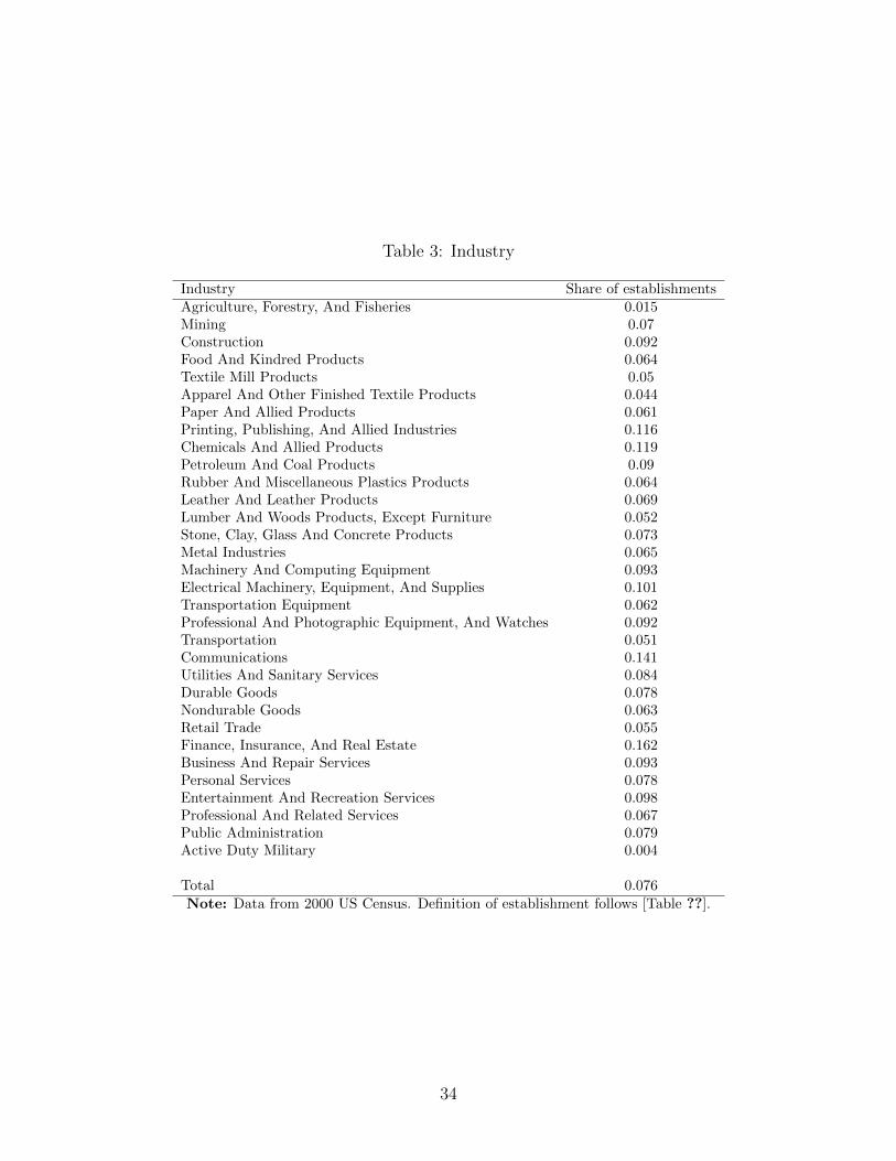
Table 3: Industry

Industry Share of establishmentsAgriculture, Forestry, And Fisheries 0.015Mining 0.07Construction 0.092Food And Kindred Products 0.064Textile Mill Products 0.05Apparel And Other Finished Textile Products 0.044Paper And Allied Products 0.061Printing, Publishing, And Allied Industries 0.116Chemicals And Allied Products 0.119Petroleum And Coal Products 0.09Rubber And Miscellaneous Plastics Products 0.064Leather And Leather Products 0.069Lumber And Woods Products, Except Furniture 0.052Stone, Clay, Glass And Concrete Products 0.073Metal Industries 0.065Machinery And Computing Equipment 0.093Electrical Machinery, Equipment, And Supplies 0.101Transportation Equipment 0.062Professional And Photographic Equipment, And Watches 0.092Transportation 0.051Communications 0.141Utilities And Sanitary Services 0.084Durable Goods 0.078Nondurable Goods 0.063Retail Trade 0.055Finance, Insurance, And Real Estate 0.162Business And Repair Services 0.093Personal Services 0.078Entertainment And Recreation Services 0.098Professional And Related Services 0.067Public Administration 0.079Active Duty Military 0.004

Total 0.076

Note: Data from 2000 US Census. Definition of establishment follows [Table ??].

34

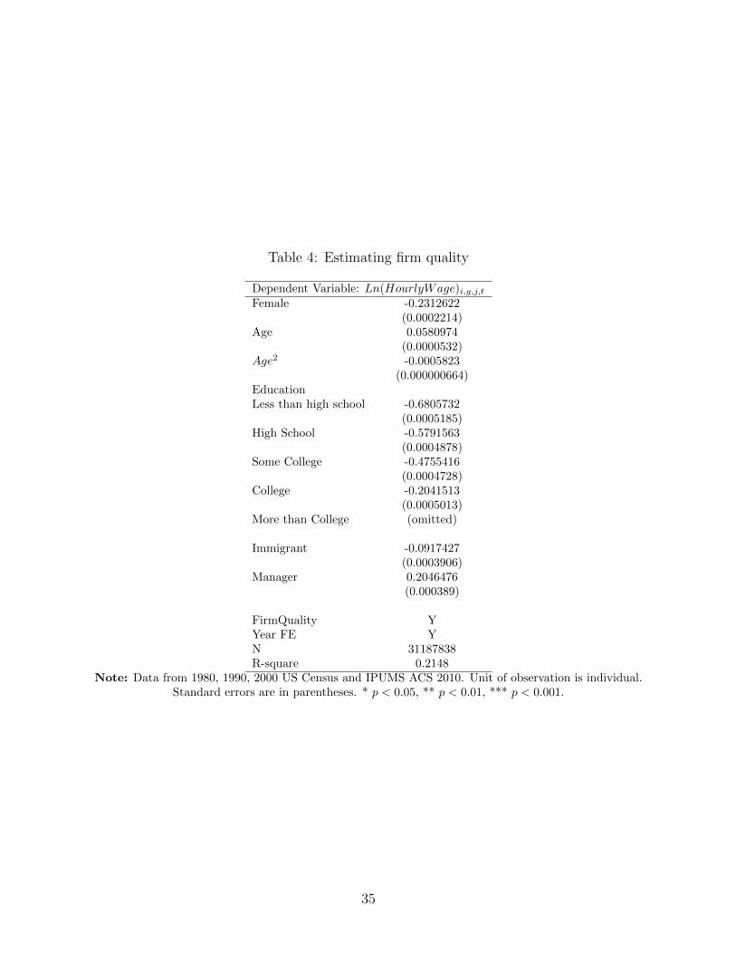
Table 4: Estimating firm quality

Dependent Variable: Ln(HourlyWage)i,g,j,tFemale -0.2312622

(0.0002214)Age 0.0580974

(0.0000532)Age2 -0.0005823

(0.000000664)EducationLess than high school -0.6805732

(0.0005185)High School -0.5791563

(0.0004878)Some College -0.4755416

(0.0004728)College -0.2041513

(0.0005013)More than College (omitted)

Immigrant -0.0917427(0.0003906)

Manager 0.2046476(0.000389)

FirmQuality YYear FE YN 31187838R-square 0.2148

Note: Data from 1980, 1990, 2000 US Census and IPUMS ACS 2010. Unit of observation is individual.Standard errors are in parentheses. * p < 0.05, ** p < 0.01, *** p < 0.001.

35

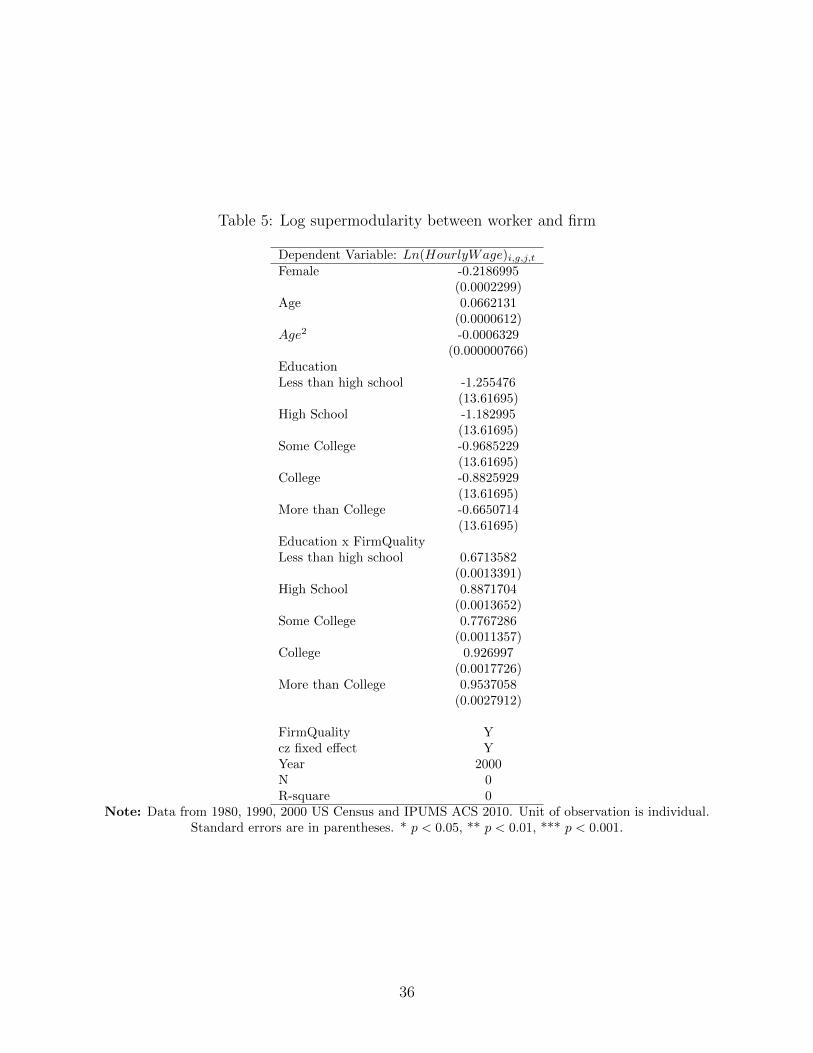
Table 5: Log supermodularity between worker and firm

Dependent Variable: Ln(HourlyWage)i,g,j,tFemale -0.2186995

(0.0002299)Age 0.0662131

(0.0000612)Age2 -0.0006329

(0.000000766)EducationLess than high school -1.255476

(13.61695)High School -1.182995

(13.61695)Some College -0.9685229

(13.61695)College -0.8825929

(13.61695)More than College -0.6650714

(13.61695)Education x FirmQualityLess than high school 0.6713582

(0.0013391)High School 0.8871704

(0.0013652)Some College 0.7767286

(0.0011357)College 0.926997

(0.0017726)More than College 0.9537058

(0.0027912)

FirmQuality Ycz fixed effect YYear 2000N 0R-square 0

Note: Data from 1980, 1990, 2000 US Census and IPUMS ACS 2010. Unit of observation is individual.Standard errors are in parentheses. * p < 0.05, ** p < 0.01, *** p < 0.001.

36

Table 6: Effect of immigrant on inequality

Dependent Variable: Inequalityg,t,10−90

Total Native Immigrant Native Manager Native WorkerImmigShareIV 0.3743*** 0.4571*** 0.2474* 0.1869* 0.4854***

(0.0861) (0.0806) (0.1212) (0.0903) (0.0875)

cz fixed effect Y Y Y Y Yyear fixed effect Y Y Y Y YN 2880 2880 2880 2880 2880R-square 0.9083 0.9114 0.7031 0.5411 0.9082

Note: Data from 1980, 1990, 2000 US Census and IPUMS ACS 2009-2011. Unit of observation iscommuting zone-industry-year. Observations are weighted, standard errors are clustered by commuting

zone, and standard errors are in parentheses. * p < 0.05, ** p < 0.01, *** p < 0.001.

Table 7: Effect of immigrant on match quality

Dependent Variable: FirmQualityg,t,pPercentile 10 30 50 70 90ImmigShareIV 0.028*** -0.039*** 0.083*** 0.030** 0.072***

(0.005) (0.008) (0.01) (0.009) (0.014)

cz fixed effect Y Y Y Y Yyear fixed effect Y Y Y Y YN 2880 2880 2880 2880 2880R-square 0.992 0.987 0.978 0.982 0.957

Note: Data from 1980, 1990, 2000 US Census and IPUMS ACS 2009-2011. Unit of observation iscommuting zone-industry-year. Observations are weighted, and standard errors are in parentheses. *

p < 0.05, ** p < 0.01, *** p < 0.001.

37

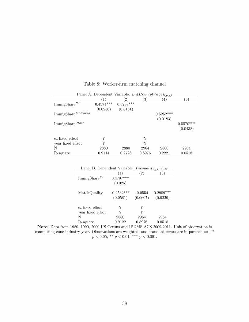
Table 8: Worker-firm matching channel

Panel A. Dependent Variable: Ln(HourlyWage)i,g,j,t(1) (2) (3) (4) (5)

ImmigShareIV 0.4571*** 0.5298***(0.0256) (0.0161)

ImmigShareMatching 0.5252***(0.0183)

ImmigShareOther 0.5570***(0.0438)

cz fixed effect Y Yyear fixed effect Y YN 2880 2880 2964 2880 2964R-square 0.9114 0.2728 0.8976 0.2221 0.0518

Panel B. Dependent Variable: Inequalityg,t,10−90

(1) (2) (3)ImmigShareIV 0.4797***

(0.026)

MatchQuality -0.2532*** -0.0554 0.2909***(0.0581) (0.0607) (0.0229)

cz fixed effect Y Yyear fixed effect Y YN 2880 2964 2964R-square 0.9122 0.8976 0.0518

Note: Data from 1980, 1990, 2000 US Census and IPUMS ACS 2009-2011. Unit of observation iscommuting zone-industry-year. Observations are weighted, and standard errors are in parentheses. *

p < 0.05, ** p < 0.01, *** p < 0.001.

38

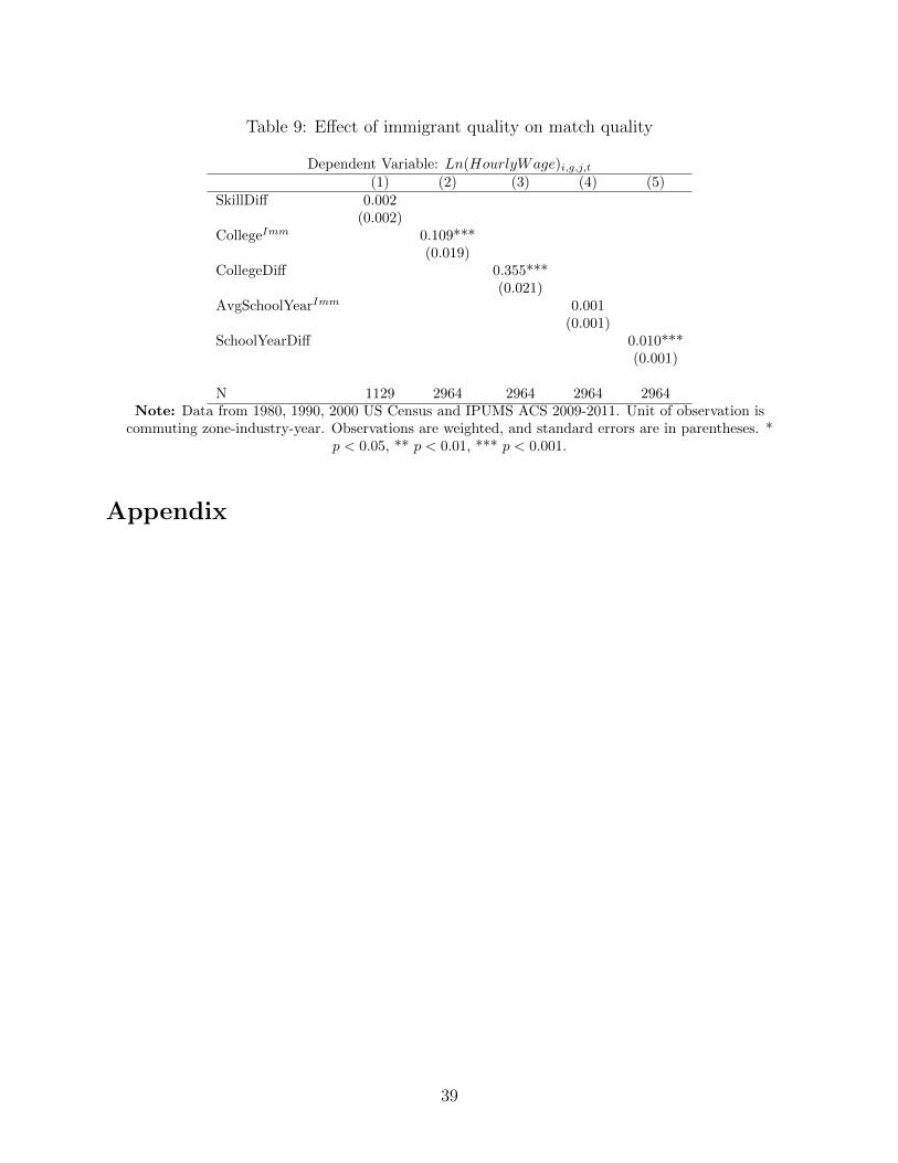
Table 9: Effect of immigrant quality on match quality

Dependent Variable: Ln(HourlyWage)i,g,j,t(1) (2) (3) (4) (5)

SkillDiff 0.002(0.002)

CollegeImm 0.109***(0.019)

CollegeDiff 0.355***(0.021)

AvgSchoolYearImm 0.001(0.001)

SchoolYearDiff 0.010***(0.001)

N 1129 2964 2964 2964 2964Note: Data from 1980, 1990, 2000 US Census and IPUMS ACS 2009-2011. Unit of observation is

commuting zone-industry-year. Observations are weighted, and standard errors are in parentheses. *p < 0.05, ** p < 0.01, *** p < 0.001.

Appendix

39

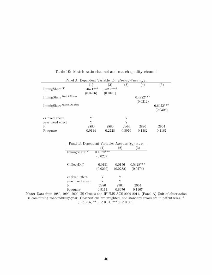
Table 10: Match ratio channel and match quality channel

Panel A. Dependent Variable: Ln(HourlyWage)i,g,j,t(1) (2) (3) (4) (5)

ImmigShareIV 0.4571*** 0.5298***(0.0256) (0.0161)

ImmigShareMatchRatio 0.4922***(0.0212)

ImmigShareMatchQuality 0.6052***(0.0306)

cz fixed effect Y Yyear fixed effect Y YN 2880 2880 2964 2880 2964R-square 0.9114 0.2728 0.8976 0.1582 0.1167

Panel B. Dependent Variable: Inequalityg,t,10−90

(1) (2) (3)ImmigShareIV 0.4579***

(0.0257)

CollegeDiff -0.0151 0.0156 0.5428***(0.0266) (0.0282) (0.0274)

cz fixed effect Y Yyear fixed effect Y YN 2880 2964 2964R-square 0.9114 0.8976 0.1167

Note: Data from 1980, 1990, 2000 US Census and IPUMS ACS 2009-2011. (Panel A) Unit of observationis commuting zone-industry-year. Observations are weighted, and standard errors are in parentheses. *

p < 0.05, ** p < 0.01, *** p < 0.001.

40

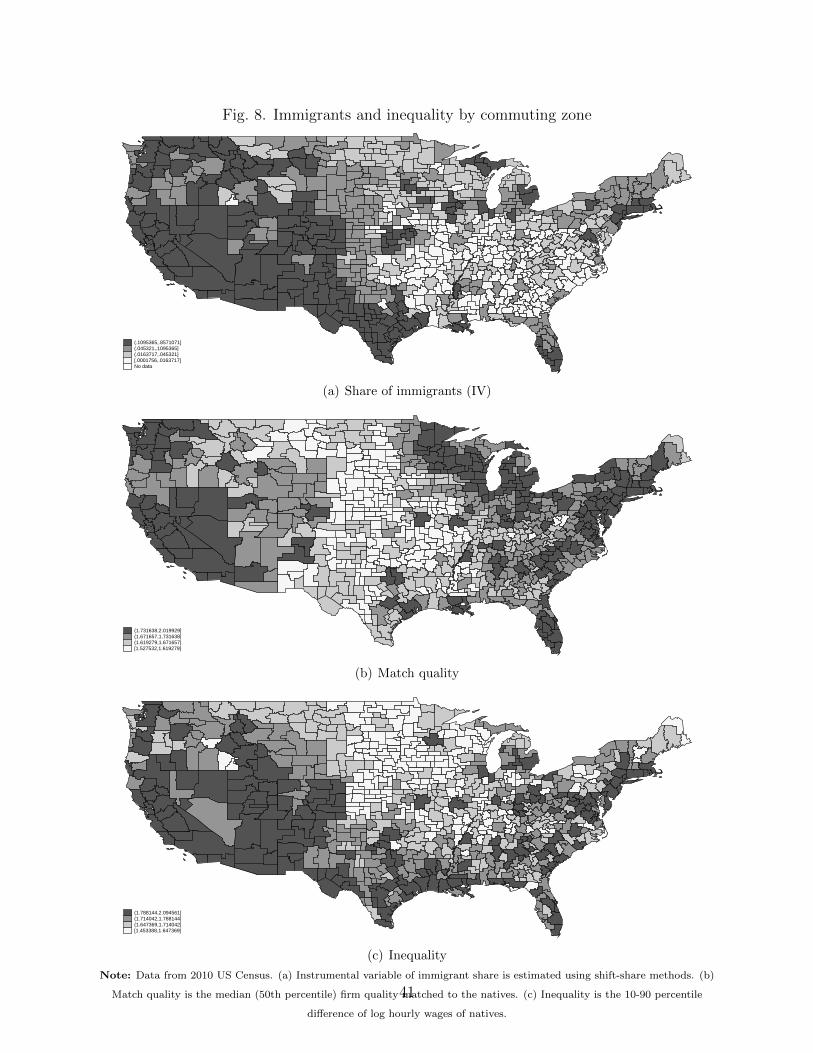
Fig. 8. Immigrants and inequality by commuting zone

(.1095365,.8571071](.045321,.1095365](.0163717,.045321][.0001756,.0163717]No data

(a) Share of immigrants (IV)

(1.731638,2.019929](1.671657,1.731638](1.619279,1.671657][1.527532,1.619279]

(b) Match quality

(1.788144,2.094561](1.714042,1.788144](1.647369,1.714042][1.453388,1.647369]

(c) Inequality

Note: Data from 2010 US Census. (a) Instrumental variable of immigrant share is estimated using shift-share methods. (b)

Match quality is the median (50th percentile) firm quality matched to the natives. (c) Inequality is the 10-90 percentile

difference of log hourly wages of natives.

41

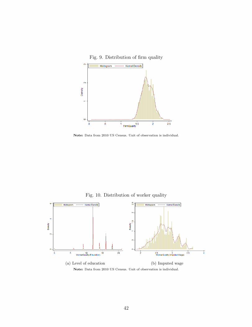
Fig. 9. Distribution of firm quality

Note: Data from 2010 US Census. Unit of observation is individual.

Fig. 10. Distribution of worker quality

(a) Level of education (b) Imputed wage

Note: Data from 2010 US Census. Unit of observation is individual.

42

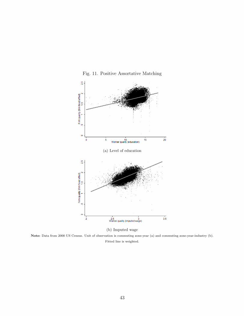
Fig. 11. Positive Assortative Matching

(a) Level of education

(b) Imputed wage

Note: Data from 2000 US Census. Unit of observation is commuting zone-year (a) and commuting zone-year-industry (b).

Fitted line is weighted.

43

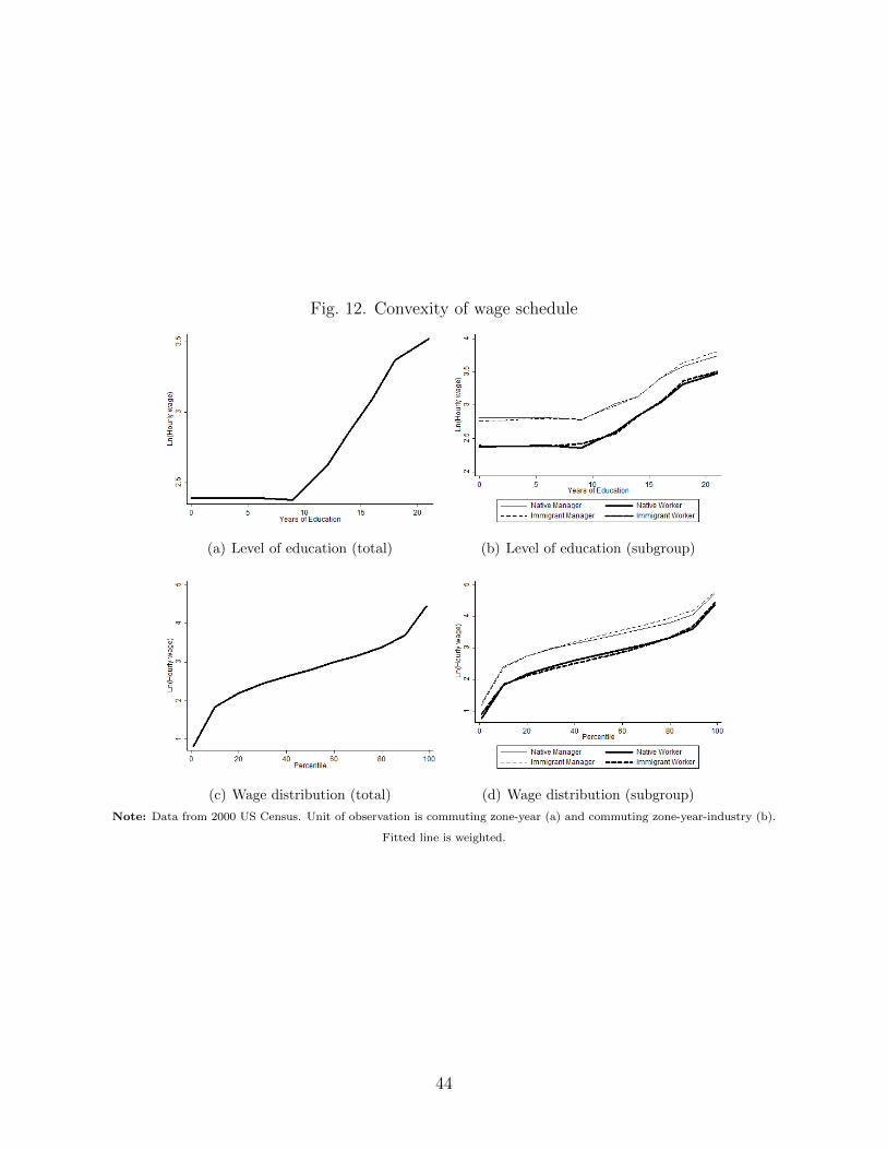
Fig. 12. Convexity of wage schedule

(a) Level of education (total) (b) Level of education (subgroup)

(c) Wage distribution (total) (d) Wage distribution (subgroup)

Note: Data from 2000 US Census. Unit of observation is commuting zone-year (a) and commuting zone-year-industry (b).

Fitted line is weighted.

44

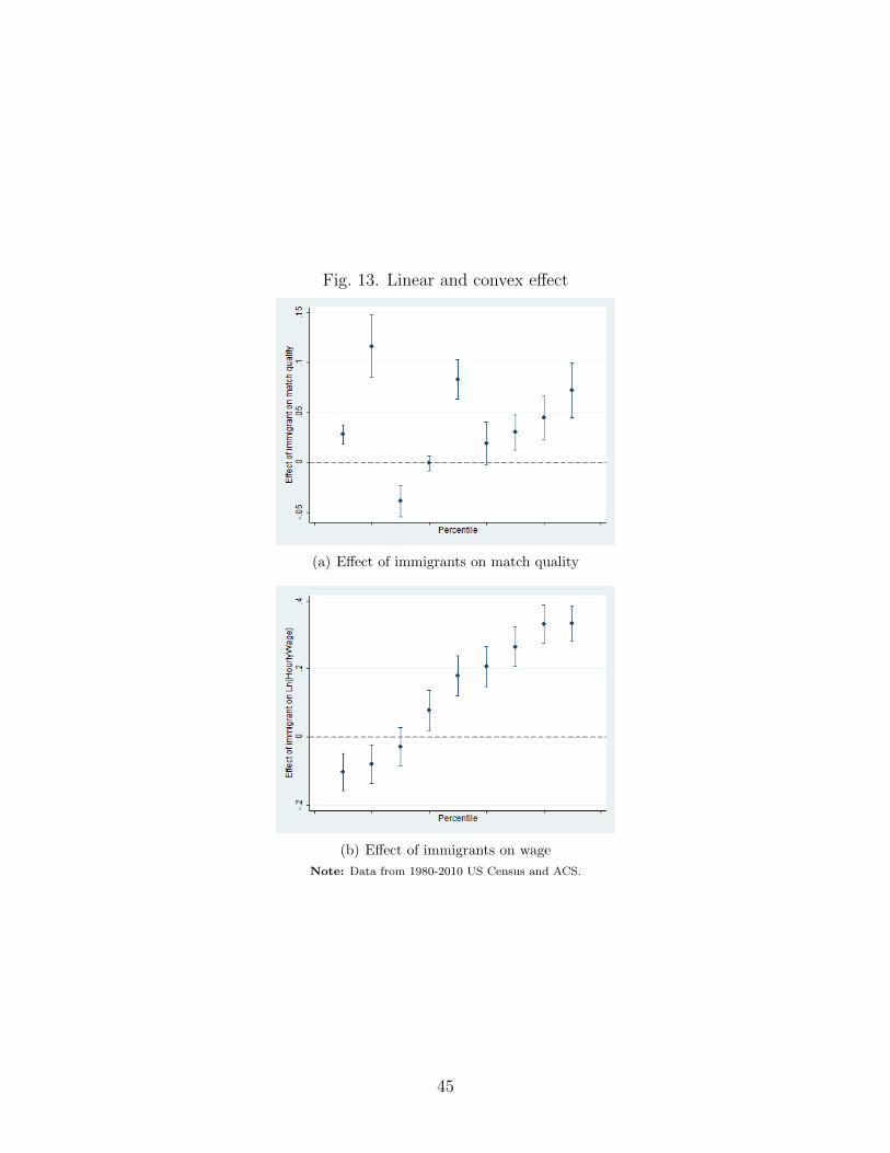
Fig. 13. Linear and convex effect

(a) Effect of immigrants on match quality

(b) Effect of immigrants on wage

Note: Data from 1980-2010 US Census and ACS.

45