Embed Size (px)
Citation preview
Impact of Financial Development
on Economic growth
Evidence from Latin America
341129
June 14, 2013
Mary-Rose G. Rosalia
Supervisor: Dr. Lorenzo Pozzi
ERASMUS UNIVERSITY ROTTERDAM
Erasmus School of Economics
Department of Economics
2
Table of Contents
Abstract .......................................................................................................................................... 5
Chapter 1 Introduction ................................................................................................................. 6
Chapter 2 Literature Review ........................................................................................................ 9
Economic Growth ..................................................................................................................... 9
Development of the Financial Sector .................................................................................... 11
Financial Sector Interaction with Economic Growth .......................................................... 13
The Case of Latin America .................................................................................................... 15
Evidence on Economic Growth and Financial Development ............................................. 17
Measurement financial development ........................................................................................ 17
Impact relationship ................................................................................................................. 18
Causal relationship ................................................................................................................. 19
Chapter 3 Methodology .............................................................................................................. 24
Empirical Specification ........................................................................................................... 24
Data .......................................................................................................................................... 25
Estimators ................................................................................................................................. 29
Fixed effects (FE) model .......................................................................................................... 29
Instrumental variables ............................................................................................................ 30
Chapter 4 Results......................................................................................................................... 32
Descriptive Statistics ............................................................................................................... 32
Fixed Effects ............................................................................................................................ 34
Instrumental Variables ............................................................................................................ 36
Robustness Analysis ................................................................................................................ 38
Chapter 5 Conclusions ................................................................................................................ 46
3
References .................................................................................................................................... 49
Appendix ...................................................................................................................................... 53
Table 9: List of Countries ....................................................................................................... 53
Table 10: Growth percentages Developed Countries ........................................................... 54
Table 11: Correlation matrix growth rates Developed Countries ....................................... 54
Table 12: FE developed countries .......................................................................................... 55
Table 13: FE-IV (1) Developed countries .............................................................................. 56
Table 14: FE-IV (2) Developed countries, G_GDP as the dependent variable ................. 57
Table 15: FE-IV (3), G_GDP as the dependent variable ..................................................... 58
Table 16: FE-IV (2), G_GNI as the dependent variable ...................................................... 59
Table 17: FE-IV (3), G_GNI as the dependent variable ...................................................... 60

4
Table of tables
Table 1: Growth percentages Latin America ............................................................................ 32
Table 2: Correlation Matrix Growth Rates Latin America ..................................................... 33
Table 3: FE Latin America, G_GDP as the dependent variable ............................................. 35
Table 4: FE-IV (1) Latin America, G_GDP as the dependent variable.................................. 36
Table 5: FE Latin America, G_GNI as the dependent variable .............................................. 39
Table 6: FE-IV (1) Latin America, G_GNI as the dependent variable................................... 40
Table 7: FE-IV (2) Latin America, G_GDP as the dependent variable.................................. 42
Table 8: Overview support for the Supply-Leading phenomenon................................................ 44
Table 9: List of Countries ........................................................................................................... 53
Table 10: Growth percentages Developed Countries ............................................................... 54
Table 11: Correlation matrix growth rates Developed Countries ........................................... 54
Table 12: FE developed countries .............................................................................................. 55
Table 13: FE-IV (1) Developed countries .................................................................................. 56
Table 14: FE-IV (2) Developed countries, G_GDP as the dependent variable ..................... 57
Table 15: FE-IV (3), G_GDP as the dependent variable ......................................................... 58
Table 16: FE-IV (2), G_GNI as the dependent variable .......................................................... 59
Table 17: FE-IV (3), G_GNI as the dependent variable .......................................................... 60
5
Abstract
In this thesis I analyze the relationship between financial development and economic growth in
Latin America. The main objective is to find evidence of the supply-leading phenomenon in the
region. The financial sector is expected to influence economic growth through its main functions
that facilitate business transactions that have a positive impact on economic growth. The analysis
is conducted with growth equations including two different financial development indicators
estimated by the fixed effects model and its extension including instrumental variables. The issue
of endogeneity is corrected for, which then allows for the proper analysis of the impact and
causal relationship between economic growth and financial development in the Latin American
countries. Data from the developing countries in Latin America and developed countries of the
OECD are used in the estimations allowing for comparisons between the two. The findings of
this study suggest that there is no considerable support for the supply-leading phenomenon in the
region which indicates a case for the demand-following phenomenon in Latin America. This
slightly differs from the findings for the developed countries where more support is found for the
supply-leading phenomenon. Moreover, the two different financial development indicators point
towards the opposite conclusion regarding the relationship between financial development and
economic growth.
Keywords: Financial development, economic growth, supply-leading phenomenon

6
Chapter 1 Introduction
The financial sector of a country is rarely mentioned as one of the major areas of improvement
for a country’s overall development. Simple transactions such as the payment of bills due occurs
probably through the financial sector. Other more complex transactions where the financial
sector is crucial for are business transactions and investments that occur through the financial
sector. Here is where the most impact could be inflicted by the financial sector’s development on
the growth of the economy (Levine, 1997).
The events in 2008 after the crash of the financial markets around the world and the added threat
of much more distress gave national governments motivation to act. They provided buyouts
larger than ever previously seen to prevent additional disasters in the financial markets that could
show spillover effects over their domestic economies and trading partners’ economies (Ivashina
& Scharfstein, 2008). These actions of the governments reflected that the financial sector should
not be ignored as it can surely impact a country’s economy. The financial sector’s development
can assist in impeding its limitation to have negative effects on their domestic economies. Thus,
the importance of the financial sector of developed countries for their economies is clear as they
experienced a recession in the periods after the global financial crisis (Reinhart & Rogoff, 2009).
There are understandable differences between developing and developed economies. It would be
interesting to assess if these differences also account for the relationship between financial
development and economic growth. The developing countries I chose to focus on are those
located in Latin America. This particular group of countries has experienced a continued increase
in the growth of their economies in the last decade. This was as a result of better policies aimed
at improving macroeconomic conditions and the positive external conditions which were the
surrounding markets (Sosa, Tsounta & Kim, 2013). According to Torre, Ize and Schmukler
(2011) the financial sector in the Latin American countries has improved considerably. It would
be interesting to know if financial development has an added value related to the growth of their
economies.
The theory regarding the relationship between economic growth and financial development has
its foundation from the main functions of the financial sector’s influence on capital accumulation

7
and the development of technologies. The financial sector facilitates business transactions that
contribute to the growth of economies (Levine, 1997). The development of the financial sector is
considered as an improvement of its main functions or additionally the reduction of barriers set
by national governments that have a negative impact on the amount of transactions conducted in
the economy (McKinnon, 1973). The theory suggested by Patrick (1966) is usually used to
describe the expectation about the causal relationship between economic growth and financial
development. The supply-leading and the demand-following phenomena are described as the
causal effect of the financial development increasing the economic growth and the economic
growth increasing the financial development respectively.
Quite a few studies were previously conducted about financial development and its possible
relationship with economic growth. Some studies focused separately on the causal relationship
and the most common evidence is from a bidirectional causal relationship between the economic
growth and the financial development of a country (Luintel & Khan, 1999; Khalifa Al-Yousif,
2002). The findings regarding the potential impact of financial development on economic growth
differ where Odedokun (1994) and Dawson (2008) found that financial development plays a
positive role in determining the economic growth. In contrast, Demetriades and Hussein (1996)
and Shan (2005) concluded that financial development has no significant effect on economic
growth. Xu (2000) and Ghirmay (2005) added more confusion on the subject by suggesting that
the financial sector’s development impact on economic growth cannot be ignored as it is vital.
Previous research conducted focusing on the Latin American region found support for both a
negative and a positive impact of financial development on economic growth. Additionally,
support was also found for both the supply-leading and the demand-following phenomena in the
previous studies (De Gregorio, 1995; Blanco, 2009). This ambiguity in the results also provided
some motivation to reassess the relationship in this region. The objective of this study is to
identify if financial development has an impact on economic growth in Latin America. Also by
making use of two different financial development indicators in the analysis of this relationship
allows for either confirming or discrediting the notion that the results are influenced by which
particular financial development indicators are used.
8
The methodology employed to analyze the problem at hand differed from the bivariate and the
multivariate Granger causality tests which are often used in the previous studies that analyzed the
relationship between financial development and economic growth. Data from 18 Latin American
countries and data from 18 developed countries for comparison purposes were used to estimate
panel regressions. I used a fixed effects model which controls for country effects for the
estimation of the growth equations that were used to analyze the impact relationship between
financial development and economic growth. An adjustment was made to account for the matter
of the suspicion of financial development’s endogeneity. This alleged endogeneity is based on
the evidence found of the bidirectional causal relationship between financial development and
economic growth from previous studies. Whether there is a case for the support of the supply-
leading phenomenon was analyzed via the fixed effects models including instrumental variables
that allowed for a one way causal relationship from financial development to economic growth.
The main findings of this study point out to some support for the supply-leading phenomenon
even though not an overwhelming one. More support nevertheless was found for the demand-
following phenomenon in the Latin American countries. The developed countries showed
slightly more evidence of the supply-leading phenomenon suggesting that there may be indeed a
difference in the relationship between financial development and economic growth for countries
at different levels of development. The use of different financial development indicators has an
influence on the results where depending on which financial development indicator is used the
conclusion regarding the supply-leading phenomenon changes. Thus, the choice of financial
development indicators should not be taken lightly.
The thesis is structured as follows; the next chapter describes the theoretical basis for the
empirical tests and summarizes the outcome of several previously conducted studies regarding
the subject. The third chapter includes the empirical specification, the description of the data and
the chosen methodology used to investigate the relationship. Subsequently, in the fourth chapter
I note the results including a robustness analysis. To finish, in the fifth chapter I conclude and
note recommendations regarding the financial development and economic growth relationship
for the Latin American region and I also note the limitations of this study.

9
Chapter 2 Literature Review
This section is regarding the relevant theory and evidence typically referred to when assessing
the relationship between financial development and economic growth. It starts with a description
of economic growth and its possible sources and continues with an outline of theories about
financial development and the possible association with economic growth. There is some focus
on Latin American countries on the subject. Next, I outline several papers by highlighting the
different methods used for analyzing these variables throughout the years. Finally, I summarize
the most notable and relevant aspects of the theory and methods relating to this relationship.
Economic Growth
Major strategic decisions and activities are carried out with the sole purpose of enhancing a
country’s economic growth. Substantial research is conducted to get a sense to what actually can
cause a country’s economy to experience a maintained growth spurt. The knowledge of the
determinants of economic growth can specify areas where should be invested in by all
stakeholders. Economic growth is a result of several different macroeconomic policies and
institutional conditions of a country. The characteristics of the economic environment where
companies engage in business transactions are determinant factors for the development of an
economy (OECD, 2004).
The aggregate production function also referred to as the neoclassical production function
developed by Solow (1957) is used to develop a source of growth equation. Total output (Y) is a
function of technology (A) usually known as total factor productivity (TFP), physical capital (K)
and labor (L). The way TFP enters the production function is known as Hicks-neutral where an
increase in the level of technological progress has no impact on the marginal products of labor
and capital (Ansari & Ahmed, 1998). Total output is the total production in a country which is
usually approximated with the gross domestic product (GDP) (Kormendi & Meguire, 1985).
(1)
Assume a Cobb Douglass function in the form of:

10
(2)
Taking natural logs and differencing with respect to time we get the equation in growth rates.
This allows for analysis of the changes in output and the contribution of physical capital and
labor to these developments. Basically changes in the level of physical capital and labor are
expected to influence changes in output. Equation (3) states that the economic growth can in
some part be explained by the growth of TFP, physical capital and labor. Here and are
elasticity measures of physical capital and labor with respect to the growth rate of the economy.
(3)
This model is used in studies attempting to analyze the determinants of economic growth. The
next step is usually estimating regression equations based on this model including other variables
that may play a significant role for economic growth depending on theories and assumptions.
The concept of economic growth is comprehensive and it is likely a result of several factors
together with what the accumulation of physical capital and labor contribute. Certain variables
that are included in the growth equation and have been found to influence economic growth
either positively or negatively are the level of education, the government’s involvement in the
economy, trade openness, legal framework and political risk (Barro, 1996, 2003).
Studies aiming to analyze financial development’s importance for economic growth use this
model including a financial development variable (F) which represents that the development of
the financial sector in some way can account for economic growth (Ansari & Ahmed, 1998;
Odedokun, 1996; Dawson, 2008). The basic model including added control variables allow for
capturing what financial development adds to economic growth, this while controlling for other
likely contributors to economic growth. Equation (6), where is the elasticity measure of the
financial development with respect to the economic growth, is crucial and it serves as basis for
empirical tests.
(4)
(5)
(6)
11
Development of the Financial Sector
The financial sector is part of the economic environment and provides a framework for carrying
out several transactions. The financial sector consists according to the International Monetary
Fund (2012) of the central bank, national banks, stock and securities markets, pension funds and
insurers. The development of these financial institutions and their services is thought to be of
great importance for a country’s development.
Ang (2008) stated that financial institutions arise as a response to transaction and information
costs in the market. Financial resources are supplied and demanded, respectively by savers and
borrowers. The act of identifying suitable savers and borrowers is costly as the matching process
without a trustworthy organization or individual to intermediate is complex. Individuals who are
willing to invest encounter difficulties when attempting to identify credible investment projects.
They are reluctant to invest before reaching reasonable agreements regarding future payouts, this
process can be time consuming and expensive. Project leaders in need of funding therefore reach
an impasse to accumulate the amount necessary for the successful advancement of their projects.
With the use of financial institutions there is a great possibility of reducing these costs. The
institutions that comprise the financial sector possess the ability to assist with the activities and
reduce costs. The specific manner in which they reduce costs is through their functions.
The financial sector main functions according to Levine (1997) are the mobilization of savings
that focuses on the collection of capital from savers intended for investments. This function is
crucial as without the efficient mobilization of savings there would be a clear constraint in the
way of the development of projects that depend on the access to these funds. Also, the financial
institutions have the ability to evaluate investment projects and point out reliable and profitable
investment opportunities. The use of financial institutions reduces the costs associated with the
selection of possible future investments which then improves the allocation of resources.
Additionally, costs are once more reduced through the use financial institutions that serve as a
middle man to lessen costs to be incurred regarding the collection of information and related to
corporate control activities after getting access to the resources. In addition, the financial sector
assists with risk management. The access of investors to different financial resources enables the
possibility of diversifying risk and this at a lower cost compared to other methods. Furthermore,

12
it helps in reducing complications for organizations and individuals that could arise when
exchanging goods, services and financial contracts.
The functions of the financial sector have in common that their objective is to reduce the costs in
activities that foster the accumulation of capital and new technologies. The development of the
financial sector entails an improvement in the quality of the functions previously mentioned. The
legal framework within which these services are provided also undergoes changes for example as
a result of new regulatory rules mandated by the government and these are also taken into
account. According to Levine (2005) modifications in the legal framework could influence the
quantity and quality of the financial services and institutions.
Ahmed and Ansari (1998) indicated that financial development can refer to financial widening
and financial deepening. The first term entails the increasing amount of financial services and
financial institutions available in a country. The second term is when there is an increase of
financial services and institutions per capita or an increase in the ratio of financial assets to
income. Financial development is also referred to as financial liberalization. McKinnon (1973)
described it as the act of minimizing distortions in the financial system. For example, prices of
the financial services provided by the financial institutions should be left up to the market
mechanism as those set by national authorities tend to be either overpriced or underpriced. The
incorrect pricing hampers the proper functioning of the financial markets. These distortions are
obstacles that clearly stand in the way of the development of the financial sector. As a result of
these distortions in the market, the amount of savings and capital accumulation decrease. This
has direct negative effects on the allocation of resources and it is not done efficiently. These
issues suggest that with financial liberalization, market transactions in the financial sector will
improve.
The financial sector’s fundamental role in the economy is becoming undeniable through the
years. Its functions’ crucial part in reducing investment costs contributes directly and indirectly
to the development of the economy as a whole. Specifically, it is expected that the benefits of
having a well-developed financial sector could positively influence the development of an
economy.
13
Financial Sector Interaction with Economic Growth
The expectation is that the financial sector is related to the economic growth through the belief
that it is essential in providing funds for capital accumulation and the development of innovative
technologies. The accumulation of capital and these technologies are fundamental drivers of the
growth of an economy. The improved or worsened characteristics of the financial sector could
have an effect on economic growth (OECD, 2004). Another major organization, the IMF (2004),
state that a dysfunctional financial sector can have effects on the function of the economy. It can
destabilize the expected effect of the chosen monetary policy, have an expansionary effect on
economic recessions and significant costs are incurred by the government when trying to save
financial institutions in financial distress. Moreover, the interdependence of countries through
finance and trade indicate that the financial crisis can have spill-over effects which were evident
after the latest financial crisis. For the reasons mentioned above the well-functioning of the
financial sector is essential for economic and financial stability.
The notable effects of financial development are the decrease of investing and saving transaction
costs as stated by Zingales (1996). This implies that the cost of capital is reduced in the domestic
economy. The financial sector assists in selection procedures by minimizing moral hazard and
adverse selection difficulties for companies. Transactions are conducted through the financial
institutions with the goal of channeling savings into profitable investments. These investments
support and lead to economic growth (Lynch, 1996). The development of the financial sector is
encouraged as one of the drivers of economic efficiency by multinational agencies and national
governments.
That there is a relationship between the growth of an economy and the development of the
financial sector may be clear but another issue arises where if in fact financial development may
lead to economic growth. This implies a causal relationship, which could either be that financial
development promotes economic growth or the opposite where economic growth promotes
financial development. The direction of the relationship could influence policies that are chosen
by local authorities. This is specifically one of the main reasons why so much time is vested in
trying to point out which one it is.
14
Patrick (1966) named the case where financial development promotes economic growth as the
supply-leading and the reverse as the demand-following phenomena. He explained further that
the demand–following phenomenon indicates that the financial sector develops in response to the
demands of the population for financial services. Thus, the development of financial services
available in the economy is a reaction to what is demanded by borrowers, investors and savers of
the population. This reflects that the financial sector is modeled after the behavior of economic
growth. This approach suggests that the financial sector is not a proactive factor in economic
growth, however it is the opposite and just manifests where the demand lies.
Furthermore, Patrick (1966) acknowledged the supply-leading phenomenon by referring to it as
the development of the financial sector before the actual demand from the population. The role
that the financial development can play according to this view is vital at the beginning of the
process. It provides a chance to stimulate growth with the aid of financial institutions. The
establishment of financial institutions and their financial services will serve as stimulation for
their use by the population to save and invest. This will in turn lead to economic growth.
Therefore, the supply of financial services by these financial institutions will stimulate economic
transactions that can lead to economic growth.
Patrick (1966) also pointed toward the possibility where the demand-following and supply-
leading phenomena would interact in practice. He suggested that an interaction between the two
is expected as the market is not static and these two views can change at any point in time as a
reaction to developments in the market transactions. The order in which these would interact is
where supply-leading would be followed by demand-following. The reason behind this order is
with the supply-leading financial institutions start up the growth process, as more transactions
are conducted and more consumers become involved, there will be an alteration to where
financial transactions are demanded. Here the shift is observed from supply-leading to demand-
following, from financial development leading economic growth to economic growth leading
financial development.

15
The Case of Latin America
The Latin American financial systems have been characterized by Stallings and Studart (2006) as
bank-based systems. These systems are set apart by the important role played by banks and the
negligible part played by capital markets for example bond markets and stock markets.
Advantages of bank-based system as explained by Diamond (1984) are that it improves the
allocation of resources and the ability of exercising corporate control is also enhanced. This is
accomplished through the use of banks who aid in reducing costs involved in monitoring and
selection procedures of firms and managers. Stulz (2000) advocated that banks assist local
companies that are in need of funding by phase of production by giving them access to external
resources. Banks and entrepreneurs engage in long term relationships where the banks commit to
give access to financial resources for future stages of the projects.
A shortcoming of these bank-based systems mentioned by Rajan (1996) is that the role played by
the banks comes with significant market power that hinders the market mechanism to function
properly. Companies’ expected profits from investments decrease considerably by the share that
belongs to the banks. Their motivation to pursue profitable investments along with lower
expected profits decreases considerably. In the absence of these projects there is a significant
shortage in a notable contribution to economic growth. Another shortcoming pointed out by
Rajan and Zingales (2001) is that the market economy might lack efficiency where prices do not
accurately reflect the costs. Specifically, banks might continue to finance projects based on
biased expectations.
A study conducted by Arestes, Demetriades and Luintel (2001) attempted to back up the
preference of one system over the other when it comes to exhibiting more influence on economic
growth. Developed countries typically have market-based financial systems. They provide the
perfect setting to compare the expected effect of market-based and bank-based financial systems
on economic growth. Their results from 10 developing countries indicate that bank-based
systems compared to market-based systems have a more significant impact on economic growth.
On the other hand, Ndikumana (2005) suggested that the two systems are complements rather
than substitutes. The results of the sample of 99 countries while controlling for country-specific
16
factors showed that the structure of the financial system has no influence on the level of impact
of financial development on economic growth.
The expectation of financial liberalization having a positive impact on economic growth did not
come through for Latin American countries. Gregorio and Guidotti (1995) investigated the
relationship between the two variables for Latin American countries around 1970’s and 1980’s.
They used panel data and growth equations including the credit level as the measurement of
financial liberalization. The results indicated that financial liberalization and economic growth
had a negative relationship for Latin American countries in that period. Thus, the elimination of
barriers in the financial markets does not have a positive impact on economic growth. They
considered that the cause of the negative effect was that the process of financial liberalization
without proper regulatory framework can impede the expected positive effects and even further
lead to a financial crisis. Alternatively, a study by Bittencourt (2012) that covered four major
countries in Latin America for the period of 1980-2007 did support the positive role of financial
development for economic growth in that region. However, this was achieved after controlling
for notable macroeconomic conditions such as government involvement in the economy and
trade openness. He noted that the positive role could have been enhanced if the national
governments took better control and avoided the hyperinflationary periods that the countries
experienced by having their institutional framework at that time improved.
The Latin American region went through some severe financial crises during the eighties and the
nineties. These crises, as any other significant financial crisis, had any significant negative
impact on the growth of the domestic economies. After these development actions were taken
with the goal to reduce the chances of these disturbances to happen again. The financial sector in
the Latin American countries has become more reliable through more variety and depth. They
experienced an increase in available banking systems and a development of the local currency
bond markets and stock markets. The financial sector is thought to be more differentiated and
complex emphasizing that institutional investors have become more significant compared with
banks. The dependability and resilient feature of the financial sector for the majority of the
countries is apparent from their reaction to the recent financial crises where they managed it
quite well (De la Torre, Ize & Schmukler, 2011).
17
Evidence on Economic Growth and Financial Development
The theory suggests that there is a relationship between financial development and economic
growth. This in essence is that development of the financial sector should have an influence on
economic growth. Furthermore, the theory proposes that an improvement in the financial
services provided by the financial institutions could lead to even more growth of the economy or
the opposite where economic growth would be the driver behind the development of the financial
sector.
Several studies were conducted attempting to find empirical proof for these ideas. The studies
are aimed at analyzing the causal and impact relationship and some researchers add the long run
view to their study by also analyzing a possible cointegrating relationship. The most recent
studies employ panel data to test these hypotheses. A clear shift is seen from using cross-
sectional data to using time series data in the analyses. This shift is a consequence of advantages
of panel data according to Levine, Loayza and Beck (2000) that are that it allows for analyzing
the financial development effect on economic growth through time for the countries. Cross-
sectional regressions tend to exhibit biased coefficient estimates, which indicate the presence of
unobserved country-specific effects that are captured in the error term. Panel data estimations are
considered superior because they control for unobserved country specific estimations. The
coefficient estimates are found to be more accurate. The use of panel data also allows for
comparisons between groups which are defined by income level or location.
Measurement financial development
The choice for the financial development variable in the relevant studies varies depending on the
countries and regions included in the study. The type of the financial system in a country,
market-based or bank-based financial systems, can be used as guidance to which financial
development indicators should be included in the analysis. For instance, when it is obvious that
the countries’ financial sector are market-based systems then an indicator capturing stock and
bond market development are included along with the usual indicators capturing the performance
of bank-based systems. The amount of financial development indicators chosen also differs
across the studies. Some researchers qualify that one variable is sufficient to capture the expected
effect of financial development in the economy. Others believe that one indicator may not

18
properly capture the level of the financial development in the country and decide to use more
than one indicator and aggregate them into one comprehensive indicator. Another option is to
make use of more than one indicator and used them to test whether having different financial
development measurement variables can influence the results. Some measurement variables that
are common to several studies are the amount of credit in the economy and the relative amount
of liquid liabilities, in some cases they are chosen as sole indicator of financial development in a
country. These two indicators measure the depth and size of the financial sector. (Gregorio &
Guidetti, 1995; see also Khadraoui & Smida, 2012).
Impact relationship
Many researchers estimate equations to determine if a particular variable has an impact on the
dependent variable. In the relevant studies a financial development variable is included as an
independent variable. This is in order to analyze the impact of the development of the financial
sector on economic growth, the dependent variable. The significance of the coefficient of the
financial development variable in these equations provides clarifications on if and what financial
development contributes to economic growth. The hypothesis of financial development not
having an impact on economic growth is widely rejected by several studies comprising of
different sample sizes, methodologies and time span.
For instance, Odedukon (1994) estimated growth equations with Ordinary Least Squares (OLS)
and Generalized Least Squares method to correct for autocorrelation when necessary. He found
that financial development plays a positive role in determining the economic growth using data
from 71 least developing countries covering the period 1964-1989. Furthermore, the equation
estimates provided support for financial development’s equal importance to economic growth
compared with other determinants of growth such as trade openness and investment share of the
economy. This contradicts the belief by some that financial development’s contribution to
economic growth is considered negligible. Additionally, Khan and Senhadji (2003) noted that
financial development has an impact on economic growth for 159 developing and industrial
countries covering the 1960-1999 period. The growth equations were also estimated by OLS
method for cross-section data and Two Stage Least Squares (TSLS) method for panel data. In
19
addition, they advise caution when choosing financial development indicators as each indicator
can display a different size effect on economic growth.
Instead of using one growth equation, Dawson’s (2008) analysis was conducted with the use of
three different growth equations. Two of the growth equations were derived from the theory of
Solow (1956) and included an investment share in the economy, the level of physical capital and
the level of labor as control variables. Each equation included a different financial development
measurement variable. The first equation includes a growth rate of the financial development
which is the growth rate of credit and the second equation includes the share of the credit in the
economy used as a proxy for its growth rate. These two equations are proved to be empirically
superior to the third equation which was not theoretically consistent. The results show that
financial development has an impact on economic growth from panel data estimations for a
group of 44 developing countries covering 1974-2001.
Khadraoui and Smida (2012) using panel data for 70 developing and developed countries over
the period of 1970-2009 estimated equations by the usual OLS, but also used the generalized
method of moments in difference and in system estimators for dynamic panel data. Their results
provided support for the notion of financial development’s positive impact on economic growth
with the use of five different measures of financial development that included two variables that
capture the credit level in the economy, liquid liabilities, market capitalization size and financial
system assets to GDP. Even with the use of a diverse choice of financial development indicators,
they still managed to conclude that financial development has a positive impact on economic
growth.
Causal relationship
Studies that attempt to analyze the causal relationship between the variables have failed to
provide unanimous support for a single hypothesis. The empirical method employed in most of
the studies is the Granger causality test. These tests employ a bivariate test framework. Some
studies’ methodology is centered on estimating the equations in vector auto-regression (VAR)
framework and from there the causal relation is deduced. The objective of verifying financial
development’s importance to economic growth has not been fulfilled by many as the common
20
result of previously conducted research is a bidirectional relationship between economic growth
and financial development. It only clarifies that there certainly is a causal relationship but the
direction is not one way, this hampers the ability of researchers to influence national policies
toward investing in the development of their financial sector with the promise of economic
growth as a result.
For instance, the study conducted by Hussein and Demetriades (1996) failed to find strong
support for financial development’s role in leading to economic growth for 16 developing
countries using a Granger causality test. They made use of two different measures of financial
development, which were both attempting to capture the level of financial intermediation in the
economy. Their conclusion was overwhelming support for bi-directionality and some for reverse
causation from their sample. Similarly, Khalifa Al-Yousif (2002) does not find convincing
support for neither supply-leading nor demand-following phenomena using Granger causality
tests in an error correction model. His different methodological approach is an attempt to deal
with the misspecification problem of models used in the studies analyzing the two variables. He
found vast proof of a bidirectional relationship between financial development and economic
growth using panel data covering 30 developing countries for the period of 1970-1999.
Then again, Christopoulos and Tsionas (2004) did find support for one of the hypotheses, the
supply-leading. Their method of choice was threshold panel cointegration tests. The threshold is
included as the level where financial development begins to have an effect on economic growth.
As the level of financial development in a country increases and reaches the threshold, then there
is a case of financial development having an impact on economic growth. Their test outcomes
suggest a one way causality relationship between financial development and economic growth, a
unidirectional relationship from financial development to economic growth. Moreover, their data
exhibited a cointegrating relationship between the variables using panel data comprising 10
developing countries for the period 1970-2000.
Developments in the methods of analyzing relationships have led to the next step in testing the
causal relationship from pairwise causality tests for testing the whole relationship in a VAR
framework. This entails estimating the financial development, economic growth and its control
21
variables in a multivariate model. The choice for analyzing a relationship in a VAR framework is
motivated by possible dynamic interrelationship between the variables (Verbeek, 2008). The
preference is to analyze macroeconomic variables in a VAR setting, this as a response to the
expected dynamic relationship between the respective variables. In the study of economic growth
and financial development, theory suggests that they exhibit a dynamic relationship where both
the supply-leading and demand-following hypotheses are possible.
Luintel and Khan’s (1999) decision to assess the relationship in a multivariate VAR followed
from their understanding shortcomings of cross-country regressions and bivariate causality tests.
Their method corrects for miss-specification problems and single equation bias from using
bivariate tests is also removed. They also found support for the bidirectional causality from the
sample employed. It is relevant to note that they found support for the same direction of the
relationship in all 10 developing countries in their sample, which is quite uncommon result in
studies of the causal association between the two variables.
Additionally, Gries, Kraft and Meierrieks (2011) contributed to the results of rejecting the notion
of financial development leading to economic growth with a sample of 13 developing countries
covering the period 1960-2003 for the majority of the countries. They found support for the
majority of the countries for the demand-following hypothesis. Adapted Granger causality tests
in a VAR and an error correction model framework were used that allowed for different lags of
the variables included in the model. They included three variables in the model specification,
trade openness together with financial development and economic growth. Regarding the
connection between the financial sector and trade they failed to find compelling support for this
relationship in promoting economic growth.
Another study that did not succeed in providing support for the supply-leading hypothesis was
conducted by Shan, Morris and Sun (2001). The hypothesis that financial development leads
economic growth is rejected with their sample of 10 developed countries for a time span of at
least 12 years. They test both the demand-following and supply-leading hypotheses with the use
of VAR that allows for controlling for possible effects of other variables that can influence both
the economic growth and financial development variables. They also found evidence of a

22
bidirectional relationship in five countries and three countries show evidence of reverse
causation. On the other hand, Xu’s (2000) study used data from 41 developing countries
covering the period 1960-1993 in a multivariate VAR framework and he discredits the notion
that financial is trivial to economic growth. The choice for analyzing the relationship in a VAR
framework allows for detection of long run total effects of financial development on economic
growth through the dynamic interactions. The level of domestic investment is included in the
estimation as a control variable. He concluded further that financial development is crucial for
economic growth and that through investments is where the most value is added from financial
development to economic growth.
An additional study by Blanco (2009) indicated no support for the supply-leading hypothesis.
The analysis was carried out using both a bivariate VAR and a multivariate VAR. The option to
perform the causality tests additionally in the multivariate VAR is to account for the possibility
of omitted variable bias in the bivariate VAR. Evidence is found for the demand-following
hypothesis for 18 countries in Latin America for the period 1962-2005. This result is supported
with the use of three financial development measurements. In order to understand this result
further the sample was divided by income levels and quality of the domestic institutional
framework. The results from tests conducted on these groups exhibited a bidirectional causality
relationship for the middle income countries and countries with a high quality institutional
framework.
Shan (2005) conducted an assessment of financial development and economic growth that
similarly provided no conclusive support for the supply-leading hypothesis in the period of 1985-
1998. If indeed the association between the two variables can be described from a causality point
of view the strength and direction is not unanimous for a group of countries. His sample
consisted of 10 OECD countries and China. The results were obtained from a VAR framework
using total credit as the sole measurement of financial development. They propose that financial
development is not one of the main drivers of economic growth as suggested by many but just a
contributing factor. Instead, Ghirmay (2004) results highlighted the case of the supply-leading
phenomenon in eight countries. He also concluded that there is a co-integrating relationship
between the two variables with the use of 13 developing countries over a time span of at least 30

23
years. The relationship was investigated in a VAR framework together with cointegration tests
and the error correction model. This supports the policy that developing countries should
improve their financial sector institutions and expect this to have an increase in the growth of
their economies as a response. Evidence is again found for a bi-directional causal relationship in
six countries from the sample.
The importance of economic growth leads to the curiosity of finding out its determinants and
whether the development of the financial sector could be one of them. The financial sector adds
value to the economy in the form of decreasing transaction and information costs associated with
carrying out investments. The financial sector of the Latin American countries has undergone
some improvement over the years but the impact of this development on economic growth is
unclear. The relationship of financial development and economic growth is analyzed mostly via
causality tests and growth equations. The studies concur that financial development has a
positive impact on economic growth. In regards to the causality, the most common result of
previous research studies with different methodologies is that both the demand-following and
supply-leading phenomena are observed from the data. It points out to a clear causal relationship
between financial development and economic growth. The aim of this study is assessing the
relationship for the Latin American region comprised of developing countries. I intend to
identify possible causal and impact relationships between the two variables and attempt to find
evidence in favor of the supply-leading phenomenon.

24
Chapter 3 Methodology
This section outlines the empirical specification, the data and the estimators used to find
evidence for the supply-leading phenomenon in Latin America. To begin with, I describe the
empirical specification with a start off point the Solow growth model mentioned in the literature
review chapter. Next, I mention and define the financial development indicators I chose for this
study. The other relevant variables included in the analysis are described. After that, I explain the
fixed effects model and its extension including instrumental variables correcting for endogeneity
that I used in the analysis.
Empirical Specification
In contrast to the preference shown in previous research for studying the relationship between
financial development and economic growth with Granger causality tests in either a bivariate or
multivariate framework, I choose to analyze the relationship with a fixed effects model with
instrumental variables. By estimating the growth equations with fixed effects, I will be able to
identify if there is any impact of financial development on economic growth while controlling
for country effects. The reason for using the instrumental variables is that they are a method for
controlling for endogeneity and making it possible to conclude in which direction the causal
relationship is. Given that the purpose of this thesis is to find evidence of the supply-leading
phenomenon which indicates that the causal relationship should be from financial development
leading economic growth.
(6)
For the analysis equation (6) which states that the growth of output also referred to as economic
growth can be explained by the growth of TFP, the growth of physical capital, the growth of
labor and the growth of financial development. First two control variables whose motivation for
being chosen are explained in the next section, (G) for the government’s involvement in the
economy and (TO) for a country’s trade openness, are added to the equation along with labor,
physical capital and the financial development variables. The growth of the government’s
involvement in the economy and the growth of a country’s openness to trade are variables that
25
are expected to have an influence on economic growth. Thus, in total five explanatory variables
are included in the model. These are expected to have some influence on economic growth. In
regards to this study, the TFP is considered as part of the residual also known in these sources of
growth equations as the Solow Residual. The Solow Residual captures all the unexplained
contributions of other sources of economic growth that cannot be identified. Several other factors
in a country could have an impact on economic growth. There are several sources of growth that
for research purposes cannot reliably be quantified. These are then captured in the error term,
which is the unexplained part in economic growth. After the inclusion of the two control
variables, government’s involvement in the economy (G) and a country’s trade openness (TO),
the error term which includes the TFP and replacing the elasticity measures with ’s we get the
following:
(7)
In the equation (7) there is the economic growth which is explained by the growth rate of several
variables. These include the growth rate of physical capital, the growth rate of labor, the growth
rate of financial development, the growth rate of the government’s involvement in the economy,
the growth rate of a country’s openness to trade and the error term that captures the unexplained
part of economic growth including in this case TFP.
Data
Subsequently, I continue with a description of the data and relevant motivation for the chosen
explanatory variables. The sample consists of 18 countries classified in the group of Latin
American countries by the World Bank. The sample also includes a group of 18 OECD countries
which are of course developed countries to use in the comparison process (see appendix table 9).
The time frame employed in this study is 1980-2011. All the annual data were collected from the
World Bank databases. The economic growth is measured by the growth rates of real GDP per
capita and real GNI per capita. Gross National Income (GNI) is considered as GDP plus receipts
from abroad for investment owned by the domestic population minus receipts owed to foreigners
from their investment in the domestic economy. Its use can be seen as complementary where it is

26
a more comprehensive account of a country’s income and therefore more suitable for comparing
countries income level (Bowen, Hollander & Viaene, 2012). Nonetheless, the use of GNI is
limited by the availability of data for the countries included in the sample.
As seen from the literature review the choice of measurements of financial development differs
between the studies and the different financial development indicators can have an impact on the
results (see Khan & Senhadji, 2003; McCaig & Stengos, 2005). In this study I chose to use two
different financial development indicators. I believe that they can truly capture the level of
development of the financial sector and also the use of two financial development indicators
allows for a comparison of the two financial development indicators on the results. The countries
in the sample are considered developing countries and have mostly bank-based financial systems
and this provided a starting point for the choice of financial development indicators (Stallings &
Studdart, 2006).
The first financial development indicator I use is the growth rate of the ratio of broad money to
GDP (G_M2). This ratio shows the extent of monetization as any other monetary aggregate. The
narrowest version of these, the M1, is considered that they fail to capture the effect of the
functions of the financial sector on the growth of an economy (Calderón & Lui, 2003). Instead,
the use of a broader version of monetary aggregates is advocated by many as the ratio quantifies
the size of the financial sector of an economy where money is used for paying and saving
purposes (Kar & Pentecost, 2000; Khalifa Al-Yousif, 2002) The ratio also refers to the financial
deepening where an increase in the ratio resembles somewhat the increase in financial services in
the economy (Odhiambo, 2008). It includes bank deposits that finance credit thus it represents
the degree of financial intermediation in the economy (Lynch, 1996).
The second financial development indicator is the growth rate of the ratio of domestic credit to
the private sector to GDP (G_DCPS). This ratio represents the section of financial development
measuring the activity of financial intermediaries where they channel resources from savers to
borrowers (Bittencourt, 2012; Beck, Demirguc-Kunt & Levine, 2000). The credit to the public
sector is not included so this ratio then represents the actions carried out by the private market
participants. Recalling that this function reduces the costs involved in investments for the
27
population, the increase in this ratio implies a direct impact on the level of investments. It then
captures directly the financial sector expected impact on economic growth (De Gregorio &
Guidetti, 1995; Khan & Senhadji, 2003). This ratio captures one activity of several from the
financial sector which could be considered a weakness, but its impact in developing countries
where it can capture the fact that domestic credit is widely used for financing local company’s
investments. These investments enhance productivity that lead to economic growth indicate that
it still is a valuable measurement of financial development (Ghirmay, 2004; King & Levine,
1993).
The other explanatory variables were selected following the literature regarding determinants of
economic growth and the availability of data (De Gregorio, 1992; De Gregorio & Guidetti, 1995;
Blanco, 2009; Bittencourt 2012). Physical capital and labor are included following the Solow
growth model and the government’s involvement in the economy and a country’s trade openness
are included additionally to capture some of the unexplained part of economic growth.
One of the most significant contributors to economic growth is the capital accumulation. This is
captured with the growth rate of physical capital (G_INV) which is measured as the growth rate
of the share of gross capital formation of GDP. This is expected to have a positive relationship
with economic growth. Physical capital also known as investment is considered crucial for the
growth of output as it assists in several ways to increasing the level of output and therefore
economic growth. Also, the increase of the productivity of workers through the more physical
capital in the form of better machines for productions that leads to lower costs of production
which can lead to an increase in the amount of production and total output in the economy
(Morgan, 1969) . An increase in the investment level can impact the level of productive labor
and this added value in facilitating and enhancing the production level leads to economic growth
(Swan, 1956).
In addition, the growth rate of labor (G_POP) is another major factor that has shown to have an
impact on countries’ economic growth. It is measured with the growth rate of the population
level following Ansari and Ahmed (1998). In the Cobb-Douglas production function derived
from the Solow growth model, an interaction between the levels of labor and physical capital
28
leads to production. The workers use the physical capital that is at their disposal in their daily
duties to produce goods and provide services. This way labor exercises influence on the level of
output and therefore economic growth. The growth rate of labor is expected to have a negative
relationship with economic growth (Mankiw, Romer & Weil, 1992). An increase in the growth
rate of labor (G_POP) which is an increase in the population implies that the available physical
capital in the domestic economy must now be spread between more individuals (Barro, 1996). It
is therefore decreasing economic growth (G_GDP) which is measured per capita.
Additionally, national governments can impact economic growth of their countries. Decisions
made by them can influence business transactions in their domestic economic environment. The
growth rate of the government’s involvement in the economy (G_GOV,) which is one of the two
control variables, is used in the attempt to capture some of the impact of the government’s
involvement in the economy. This is measured with the growth rate of the share of general
government consumption expenditure of GDP (Ergungor, 2004). It includes the costs of products
and services acquired by the government. Salaries of employees in the service of the government
and expenses for national security and defense excluding military related costs are also included
in this expenditure. An increase in government rules and regulations are expected to have a
negative relationship with economic growth. The government can through its policies, exercise
significant influence on the economic environment. Measures such as an increase in corporate
income tax taken following taxation policies can have a negative impact on business transactions
in the economy. Moreover, government spending is seen sometimes as decreasing productivity
of the domestic market instead of enhancing it for example with policies regarding international
trade that can have opposite effects reducing economic growth (Barro, 1996).
Finally, the growth rate of the degree of the country’s openness to trade (G_TO) is the other
control variable chosen and it is expected to positively influence the level of economic growth
(Khadraoiuh & Smida, 2012; Bittencourt, 2012). It is measured as the growth rate of the share of
exports plus imports to GDP (Moral-Benito, 2009). There are gains of engaging in international
trade signifying the mutual engagement in trading products and services between countries will
lead to benefits for every country involved captured in the growth of their economies. However,
certain groups within the engaging countries can also lose. A country’s openness to trade may

29
influence the domestic distribution of income where there are winners and losers from trade. The
relevant part here is with the redistribution of the gains of trade where the losers of trade can be
compensated and therefore allowing the final result to be a positive one for the economy as a
whole (Krugman & Obstfelt, 2009)
Estimators
Next, I describe the two estimators, fixed effects and fixed effects with instrumental variables,
used in the analysis.
Fixed effects (FE) model
This model is used to analyze the impact of variables over time. It analyzes the relationship
between the explanatory variables and the dependent variable within a cross-section, in this case
a country. The sample consists of several cross-sections, 18 countries to be exact in this analysis.
It is quite reasonable that individual characteristics of each cross-section could and will influence
the dependent variable. This influence creates bias on the dependent variable and the coefficient
estimates if not taken into account. This is corrected for by introducing fixed effects in the OLS
estimation. Equation (7) which includes the economic growth as the dependent variable, and the
growth rates of the five variables as the independent variables, this equation is transformed to
include the fixed effects resulting in equation (8).
(8)
The intercept term is varies per cross-section but not per time. It captures all observable and
unobservable time-invariant differences across the individual countries. is the dependent
variable economic growth. is a vector of the explanatory variables which include the growth
rate of the financial development indicators, growth rate of broad money as share of GDP
(G_M2) or the growth rate of the ratio of the domestic credit to the private sector as share of
GDP (G_DCPS). The vector includes also the growth rates of the other explanatory variables,
growth rate of physical capital (G_INV), growth rate of labor (G_POP), the growth rate of the

30
government’s involvement in the economy (G_GOV) and the country’s openness to trade
(G_TO).
Equation (8) is supposed to serve for analyzing the impact of financial development on economic
growth. However, finding evidence for the supply-leading phenomenon necessitates one more
adjustment in order to be certain that the estimation is capturing the desired relationship from
financial development influencing economic growth and not the opposite. This is possible when
correcting for endogeneity with instrumental variables.
Instrumental variables
In order for the equation (8) to provide consistent and unbiased coefficients a key requirement is
that the explanatory variables should be exogenous [ E ( )=0] . The use of instrumental
variables (IV) is suggested to correct for the correlation between the independent variables and
the error term and reduce the bias on the estimated coefficients induced by endogeneity. The
independent variables should not be correlated with the error term as this implies a bi-directional
causal relationship between the independent variables and the dependent variable.
Quite some evidence is found of the bi-directional causality relationship between financial
development and economic growth in the previous studies (see Hussein & Demetriades, 1996;
Luintel & Khan, 1999; Khalifa Al-Yousif, 2002; Shan, Morris & Sun, 2001). This suggests that
the estimation of the growth equations based solely on the supply-leading phenomenon without
correcting for the endogeneity of the financial development’s variable would have as a result
biased and inconsistent coefficients. The financial development’s variable endogeneity brings
along shortcomings to the growth equations if not properly controlled for. A case can also be
made for the endogeneity of the other explanatory variables. If this is so this must also be
controlled for.
When the independent variables are correlated with the error term , they are considered
endogenous. In order to correct for this endogeneity the option is to find other variables that
are correlated with the independent variables but not correlated with the error term , these
variables are then considered exogenous.

31
(9)
(10)
A regression is estimated with the endogenous variables as the dependent variable and the IV’s
as the independent variables. The fitted values of this regression are then included in the
original regression instead of the endogenous variables. This method is known as TSLS. This
estimation method allows for analyzing the intended relationship with consistent and unbiased
coefficient estimates according to OLS.
The regression equation becomes:
(11)
The economic growth is now explained by the fitted values of the growth rates of the
independent variables and an error term. The TSLS estimation method provides a way to
estimate the relevant growth equation based on the supply-leading phenomenon. The results
from this estimation could either verify or reject this hypothesis. The endogeneity of the financial
development variable is controlled for and so making sure that the analyzed impact is only from
financial development leading economic growth. By including IV’s for the other explanatory
variables other possibilities of endogeneity are also taken care off.
The search for proper IV’s is quite challenging because of the threat of using weak or invalid
instruments that will have inefficient estimates than OLS as a result. A common option in the
literature is the use of lagged values of explanatory variables as the instruments (Barbosa &
Eiriz, 2009). These values from previous periods are not expected to be correlated with the
current error term and their relations to the explanatory variables are basic reasons why they are
chosen as IV’s. In this study I choose to use lagged values as IV’s and I will use three different
instrument sets (Cheng & Kwan, 2002).
32
Chapter 4 Results
In this section I present the outcome of the estimations assessing the financial development and
economic growth relationship. Some descriptive statistics are stated with the purpose of shining
some light on financial development and economic growth of the Latin American countries.
Subsequently, I continue with the different growth equations and their estimations using IV’s.
Similar projections are carried out with data from the developed countries whose tables are
available in the appendix. These are done in order to provide a benchmark for the Latin
American countries. To finish, a different measure of economic growth and different instrument
sets are used for the estimations with the purpose of analyzing the robustness of the findings.
Descriptive Statistics
Table 1: Growth percentages Latin America
G_DCPS G_M2 G_GDP G_GNI G_INV G_POP G_TO G_GOV
Mean 0.009 0.016 0.011 0.011 -0.001 0.017 0.011 0.003
Maximum 1.175 0.827 0.151 0.142 1.006 0.035 1.094 1.513
Minimum -1.110 -1.298 -0.164 -0.256 -0.895 -0.009 -0.558 -0.854
Std. Dev. 0.191 0.171 0.043 0.052 0.172 0.008 0.132 0.134 Note: This table includes the summary values including the mean and standard deviation of the growth rate of the
ratio of domestic credit to the private sector to GDP (G_DCPS), the growth rate of the ratio of broad money to GDP
(G_M2), the growth rate of real Gross Domestic Product per capita (G_GDP), the growth rate of real Gross National
Income per capita, the growth rate of physical capital (G_INV), the growth rate of labor (G_POP) and the growth
rate of government’s involvement in the economy (G_GOV). These values are calculated from the common sample
of 18 Latin American countries.
In table 1 it is seen that every variable has a positive mean percentage of growth except for
physical capital which is not growing at all. The growth percentages are less than one percent per
year for both the developing and the developed countries’ sample. The growth of labor has the
highest mean growth percentage of all the variables to be included in the model. From the two
financial development indicators, G_M2 has the highest mean growth percentage. The financial
development indicators and GDP growth for the developed countries (see appendix table 10)
show higher mean growth percentages compared to the Latin American countries. Additionally,
the G_DCPS financial development indicator has the highest mean percentage of the variables to
be included in the model for the developed economies.

33
The summary statistics above provide a start for the assessment of the relationship and possible
differences between countries with different levels of development. The differences in economic
growth were expected which is one of the criteria used by the World Bank in the classification of
the countries in groups by level of development. In addition, the higher growth percentages of
the financial development indicators for the developed countries also corroborate their status as
countries with a higher level of development. The next step is to explore if there is the possibility
of an existing linear relationship between financial development and economic growth. This can
provide some insight regarding a possible impact relationship. The correlation values and their
potential statistical significance can at least verify the presence of a linear relationship.
Table 2: Correlation Matrix Growth Rates Latin America
G_DCPS G_M2 G_GDP G_GNI G_INV G_POP G_TO G_GOV
G_DCPS 1
G_M2 0.582*** 1
G_GDP 0.100** 0.036 1
G_GNI 0.123*** 0.086* 0.908*** 1
G_INV 0.100** 0.107** 0.461*** 0.401*** 1
G_POP -0.031 -0.005 -0.158*** -0.189*** -0.027 1
G_TO -0.007 0.043 -0.001 -0.155*** 0.255*** -0.056 1
G_GOV 0.311*** 0.297*** 0.057 0.076 0.055 -0.020 -0.022 1
Note: *, **, ***, reflects significance at the 10%, 5% and 1% level. These are the Pearson correlation values of the
variables to be included in the models with each other. The variables are the growth rate of the ratio domestic credit
to the private sector to GDP (G_DCPS), the growth rate of the ratio of broad money to GDP (G_M2), the growth
rate of real GDP per capita (G_GDP), the growth rate of real GNI per capita, the growth rate of physical capital
(G_INV), the growth rate of labor (G_POP) and the growth rate of the government’s involvement in the economy
(G_GOV).
The relevant figures in the matrix above suggest that there is a linear relationship between
financial development and economic growth. Nonetheless, from the size of the correlation
statistic this linear relationship is considered a weak one. Both financial development indicators
are positively correlated with G_GDP, but for only G_DCPS this correlation is statistically
significant. The strength of the positive linear relationship between G_DCPS and G_GDP is
weak. Both financial development indicators have a statistically significant correlation with GDP
growth in the developed countries (see appendix table 11). Both the growth of the country’s
openness to trade and the growth of the government’s participation in the economy have no

34
statistically significant linear relationship with economic growth in Latin America. In the case of
the developed countries there is evidence of a highly statistically significant linear relationship
with the G_GDP for both financial development indicators. A statistically significant positive
linear relationship between economic growth and physical capital growth is seen for both the
developing and the developed countries. This points out once again to their positive association.
Regarding the linear relationship between the growth of labor and economic growth there is no
difference for the developed and developing countries where both groups exhibit a statistically
significant negative one as suggested by Solow (1956).
Fixed Effects
Consequently, I proceed with the estimations based on equation (9). A total of three models are
estimated which include the two basic estimations, each time including one of the financial
development indicators and the third one including both of the financial development indicators.
The equations were estimated when necessary with White robust standard errors to account for
autocorrelation which is not unusual in regressions estimated with time series data.
In table 3 on the following page it is seen that in all three models that financial development has
no statistically significant impact on economic growth in Latin America. None of the financial
development indicators are found to be statistically significant. The models estimated with the
developed countries' data (see appendix table 12) show not statistically significant coefficients
for all the financial development indicators included in the three models. Instead, the growth of
physical capital has a statistically significant positive impact on economic growth in all the
models for both the developed and the developing countries which support the importance of
capital accumulation for economic growth for all countries at different levels of development. An
increase in the growth of labor has a statistically significant negative impact on economic growth
for both the developing and the developed countries. The growth of a country’s openness to trade
is not statistically significant in both the developing and the developed countries. The growth of
the government’s involvement in the economy has no statistically significant impact on the
growth of developing economies, but it does have a highly statistically significant negative
impact on the growth of the developed economies.

35
Table 3: FE Latin America, G_GDP as the dependent variable
I II III
G_DCPS 0.007
(0.55)
0.015
(1.07)
G_M2 -0.007
(-0.50)
-0.015
(-1.01)
G_INV 0.122***
(6.85)
0.123***
(7.10)
0.122***
(6.94)
G_POP -2.271***
(-3.36)
-2.276***
(-3.39)
-2.261***
(-3.38)
G_GOV 0.002
(0.14)
0.008
(0.63)
0.005
(0.32)
G_TO -0.048
(-1.48)
-0.049
(-1.56)
-0.047
(-1.46)
2 0.28 0.28 0.31
F-statistic 10.53 10.56 10.16
DW-statistic 1.36 1.35 1.36
N 538 541 538
Note: *, **, ***, reflects significance at the 10%, 5% and 1% level, t-statistic based on White standard errors given
in parenthesis. The adjusted R squared, the F-statistic, the Durbin Watson statistic and the amount of observations
are stated. Economic growth measured with the real GDP per capita (G_GDP) is the dependent variable. The
explanatory variables in all the estimations are the growth rates of the following variables, physical capital (G_INV),
labor (G_POP), the government’s involvement in the economy (G_GOV) and the country’s trade openness (G_TO).
The growth rates of these financial development indicators are included; in model (I) the ratio of the domestic credit
to the private sector to GDP (G_DCPS), in model (II) the ratio of broad money to GDP (G_M2); in model (III) both
(G_DCPS) and (G_M2)
Based on the results stated, I fail to reject the hypothesis of financial development growth having
no impact on economic growth. This suggests that the development of the financial sector in
Latin American countries has no statistically significant influence on economic growth. The
financial sector’s development similarly has no statistically significant impact on economic
growth in the developed countries, suggesting that regarding this matter there is no obvious
difference between the developed and the developing countries. These results of the financial
development having no impact on economic growth are not encouraging for the next step of
finding evidence of the supply-leading phenomenon however biased caused by endogeneity in
the equations could have been one reason for this matter where not statistically significant
coefficients were found for the financial development indicators.

36
Instrumental Variables
Next, the equations were re-estimated with IV’s to control for the alleged endogeneity present in
the equations. So, allowing the focus to lie on investigating the presence of the supply-leading
phenomenon in this region.
Table 4: FE-IV (1) Latin America, G_GDP as the dependent variable
I II III
G_DCPS 0.139
(1.20)
0.138
(1.33)
G_M2 -0.040
(-0.72)
-0.128**
(-2.31)
G_INV 0.123***
(2.96)
0.111***
(3.11)
0.122***
(3.25)
G_POP -1.472
(-1.57)
-1.937**
(-2.02)
-1.326
(-1.44)
G_GOV 0.019
(0.23)
0.084
(1.28)
0.132
(1.80)
G_TO -0.151
(-0.73)
-0.144
(-1.16)
-0.128
(-0.70)
F-statistic 3.21 2.89 3.47
DW-statistic 1.94 1.60 1.89
N 497 502 497
Note: *, **, ***, reflects significance at the 10%, 5% and 1% level, t-statistics based on White standard errors are
given in parenthesis. The F-statistic, Durbin Watson statistic and number of observations are stated. Economic
growth measured by the growth of real GDP per capita (G_GDP) is the dependent variable. The first instrument set
lagged values of the explanatory variables (-1 to -2) is used. The explanatory variables in all the estimations are the
growth rates of the following variables, physical capital (G_INV), labor (G_POP), government’s involvement in the
economy (G_GOV) and the country’s trade openness (G_TO). The growth rates of these financial development
indicators are included; in model (I) the ratio of the domestic credit to the private sector to GDP (G_DCPS), in
model (II) the ratio of broad money to GDP (G_M2); in model (III) both (G_DCPS) and (G_M2)
To begin with, I note that from table 4 above it is clear that in the developing countries the
growth of the government’s involvement in the economy and the growth of a country’s openness
to trade are again not statistically significant. In addition, the growth of physical capital in the
developing countries has once more a statistically significant impact on economic growth in the
estimations using IV’s. The growth of labor now only has a statistically significant negative
impact in model (II). Additionally to these there is now the growth of financial development also
37
having a statistically significant impact on economic growth. Model (III) has a statistically
significant financial development indicator however its minus sign suggests a negative impact
from financial development on economic growth. Model (III) included both G_DCPS and G_M2
but only the latter was statistically significant. If G_M2 increases by 1% this causes a decrease of
0.13% growth of the economy on average.
I find that there is no support for the supply-leading phenomenon in this region based on two
models with not statistically significant coefficient for the financial development indicators and
the third one with a negative statistically significant coefficient which show no support for the
hypothesis of financial development leading economic growth. The negative relationship
between financial development and economic growth is also found in a study by Gregorio and
Guidetti (1995). The negative impact of the developments in the financial sector could be seen as
a result of non-well-functioning set of financial institutions and organizations. The functions of
the financial sector are not well carried out and then it obstructs smoothing business transactions
aimed to increase the amount of investments and technologies that can enhance economic growth
in the Latin American countries. From the developed countries sample (see appendix table 13)
there is a slight support for the supply-leading phenomenon. Model (I) has a slight statistically
significant positive coefficient for the G_DCPS financial development indicator. The three
models now only show a statistically significant role of the physical capital growth for the
growth of the developed economies. The growth of labor and the growth of the government’s
participation in the economy are not statistically significant anymore.
The results of the FE-IV estimations do not provide support for the supply-leading phenomenon
in Latin America. The financial development indicators have not statistically significant
coefficients in all the estimations. Therefore financial development is not leading economic
growth in Latin America. There seems to be a slight difference between the developing and the
developed countries regarding the relationship between financial development and economic
growth. For the developed countries support is found for the supply-leading phenomenon from
one third of the models. Thus, in the developed countries the development of the financial sector
has a statistically significant impact on economic growth and leads to a higher GDP per capita
whereas in the group of developing countries in Latin America there is less evidence for this
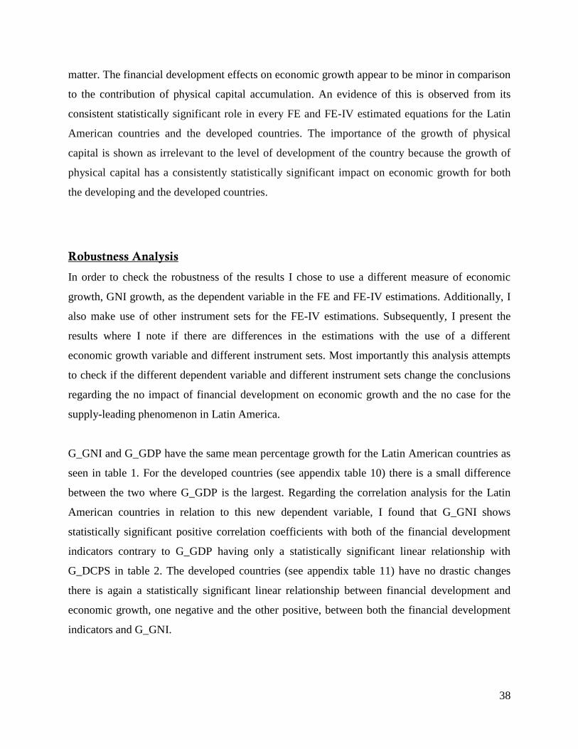
38
matter. The financial development effects on economic growth appear to be minor in comparison
to the contribution of physical capital accumulation. An evidence of this is observed from its
consistent statistically significant role in every FE and FE-IV estimated equations for the Latin
American countries and the developed countries. The importance of the growth of physical
capital is shown as irrelevant to the level of development of the country because the growth of
physical capital has a consistently statistically significant impact on economic growth for both
the developing and the developed countries.
Robustness Analysis
In order to check the robustness of the results I chose to use a different measure of economic
growth, GNI growth, as the dependent variable in the FE and FE-IV estimations. Additionally, I
also make use of other instrument sets for the FE-IV estimations. Subsequently, I present the
results where I note if there are differences in the estimations with the use of a different
economic growth variable and different instrument sets. Most importantly this analysis attempts
to check if the different dependent variable and different instrument sets change the conclusions
regarding the no impact of financial development on economic growth and the no case for the
supply-leading phenomenon in Latin America.
G_GNI and G_GDP have the same mean percentage growth for the Latin American countries as
seen in table 1. For the developed countries (see appendix table 10) there is a small difference
between the two where G_GDP is the largest. Regarding the correlation analysis for the Latin
American countries in relation to this new dependent variable, I found that G_GNI shows
statistically significant positive correlation coefficients with both of the financial development
indicators contrary to G_GDP having only a statistically significant linear relationship with
G_DCPS in table 2. The developed countries (see appendix table 11) have no drastic changes
there is again a statistically significant linear relationship between financial development and
economic growth, one negative and the other positive, between both the financial development
indicators and G_GNI.
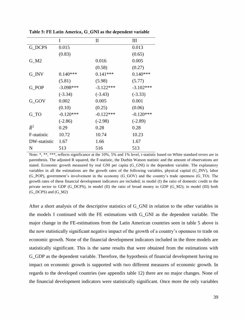
39
Table 5: FE Latin America, G_GNI as the dependent variable
I II III
G_DCPS 0.015
(0.83)
0.013
(0.65)
G_M2 0.016
(0.58)
0.005
(0.27)
G_INV 0.140***
(5.81)
0.141***
(5.98)
0.140***
(5.77)
G_POP -3.098***
(-3.34)
-3.122***
(-3.43)
-3.102***
(-3.33)
G_GOV 0.002
(0.10)
0.005
(0.25)
0.001
(0.06)
G_TO -0.120***
(-2.86)
-0.122***
(-2.98)
-0.120***
(-2.89)
2 0.29 0.28 0.28
F-statistic 10.72 10.74 10.23
DW-statistic 1.67 1.66 1.67
N 513 516 513
Note: *, **, ***, reflects significance at the 10%, 5% and 1% level, t-statistic based on White standard errors are in
parenthesis. The adjusted R squared, the F-statistic, the Durbin Watson statistic and the amount of observations are
stated. Economic growth measured by real GNI per capita (G_GNI) is the dependent variable. The explanatory
variables in all the estimations are the growth rates of the following variables, physical capital (G_INV), labor
(G_POP), government’s involvement in the economy (G_GOV) and the country’s trade openness (G_TO). The
growth rates of these financial development indicators are included; in model (I) the ratio of domestic credit to the
private sector to GDP (G_DCPS), in model (II) the ratio of broad money to GDP (G_M2); in model (III) both
(G_DCPS) and (G_M2)
After a short analysis of the descriptive statistics of G_GNI in relation to the other variables in
the models I continued with the FE estimations with G_GNI as the dependent variable. The
major change in the FE-estimations from the Latin American countries seen in table 5 above is
the now statistically significant negative impact of the growth of a country’s openness to trade on
economic growth. None of the financial development indicators included in the three models are
statistically significant. This is the same results that were obtained from the estimations with
G_GDP as the dependent variable. Therefore, the hypothesis of financial development having no
impact on economic growth is supported with two different measures of economic growth. In
regards to the developed countries (see appendix table 12) there are no major changes. None of
the financial development indicators were statistically significant. Once more the only variables
40
that have a statistically significant impact on economic growth are the growth of physical capital,
the growth of labor and the growth of the government’s involvement in the economy.
Next the FE IV’s were estimated with G_GNI as the dependent variable allowing for finding
evidence for the supply-leading phenomenon in Latin America. The IV-estimations results noted
in table 6 below indicate no support for the supply-leading phenomenon in the Latin American
region. This finding is similar to the results found with G_GDP as the dependent variable.
Table 6: FE-IV (1) Latin America, G_GNI as the dependent variable
I II III
G_DCPS 0.142
(1.48)
0.104
(1.26)
G_M2 0.046
(0.60)
-0.008
(-0.09)
G_INV 0.144***
(2.73)
0.175***
(2.62)
0.166***
(3.16)
G_POP -2.105
(-1.11)
-3.054
(-1.25)
-2.096
(1.14)
G_GOV 0.088
(0.56)
0.167
(1.18)
0.156
(-1.19)
G_TO -0.481**
(-2.08)
-0.641**
(-2.49)
-0.488**
(-2.39)
F-statistic 3.93 3.59 3.87
DW-statistic 2.02 2.08 2.07
N 474 479 474
Note: *, **, ***, reflects significance at the 10%, 5% and 1% level, t-statistic based on White standard errors are
given in parenthesis. The F-statistic, Durbin Watson statistic and amount of observations are noted. Economic
growth measured by real GNI per capita (G_GNI) is the dependent variable. The instrument set is lagged values of
the explanatory variables (-1 to -2). The explanatory variables in all the estimations are the growth rates of the
following variables, physical capital (G_INV), labor (G_POP), government’s involvement in the economy
(G_GOV) and the country’s trade openness (G_TO). The growth rates of these financial development indicators are
included; in model (I) the ratio of the domestic credit to the private sector to GDP (G_DCPS), in model (II) the ratio
of broad money to GDP (G_M2); in model (III) both (G_DCPS) and (G_M2)
All the financial development indicators in the models have coefficients that are not statistically
significant. The growth of physical capital, the growth of labor and the growth of a country’s
trade openness remain having a statistically significant impact on economic growth in the region.
For the developed countries (see appendix table 13) there is now no support from the models for
41
the supply-leading phenomenon. None of the coefficients for the financial development
indicators were statistically significant. The growth of labor is slightly statistically significant in
model (I). The only variable to have a statistically significant impact on economic growth in all
the three models is the growth of physical capital.
In short, the first attempt of a robustness check showed that the result of financial development
having no impact on economic growth is supported with two different economic growth
variables. The lack of support for the supply-leading phenomenon in Latin America is supported
by the use of two different economic growth measures. In order to investigate further the supply-
leading phenomenon in Latin America, the models were estimated with IV’s using two more
instrument sets. First, the instrument sets were used in the FE-IV with economic growth
measured by G_GDP as the dependent variable. Then, the same is done but this time economic
growth is measured by G_GNI as the dependent variable. These results can provide additional
backup to conclusions regarding the supply-leading phenomenon in the Latin American region
and apparent differences with the group of the developed countries.
The outcomes of the models estimated with G_GDP as the dependent variable and the second
instrument set lagged values of the explanatory variables (-1 to -3) showed no evidence of the
supply-leading phenomenon in Latin America. Model (III) in table 7 on the following page
shows a statistically significant negative impact of financial development on economic growth.
A 1% increase in G_M2 causes a 0.09% decrease in economic growth. This is the opposite of the
supply-leading phenomenon because the financial development is influencing the growth of the
economy but it results in a decrease instead of an increase of its growth level. The growth of
physical capital is the only variable that is statistically significant in all the three models. The
growth of labor, the growth of a country’s trade openness and the growth of the government
participation in the economy are not statistically significant in all models. Therefore, no support
is found for the supply-leading phenomenon in Latin America with G_GDP as the dependent
variable and the two different instrument sets. In all the three models for the developed countries
support is shown for the supply-leading phenomenon (see appendix table 14). The growth of
physical capital is once more statistically significant in all the three models whereas the growth
of labor has only a slightly statistically significant impact on economic growth in model (II). The

42
growth of the government’s participation in the economy has no statistically significant impact
on economic growth in the three models and the growth of a country’s trade openness has a
statistically significant impact which is negative in model (III).
Table 7: FE-IV (2) Latin America, G_GDP as the dependent variable
I II III
G_DCPS 0.107
(1.04)
0.084
(1.00)
G_M2 -0.039
(-0.81)
-0.094*
(-1.79)
G_INV 0.116**
(2.17)
0.102**
(2.52)
0.117**
(2.72)
G_POP -1.910
(-1.36)
-2.182
(-1.51)
-1.802
(-1.43)
G_GOV -0.033
(-0.50)
0.016
(0.18)
0.055
(0.80)
G_TO -0.312
(-1.51)
-0.303
(-1.61)
-0.256
(-1.54)
F-statistic 3.19 3.27 3.28
DW-statistic 1.94 1.76 1.83
N 477 483 477
Note: *, **, ***, reflects significance at the 10%, 5% and 1% level, t-statistics based on White standard errors given
in parenthesis. The F-statistic, Durbin Watson statistic and amount of observations are noted. Economic growth
measured by real GDP per capita (G_GDP) is the dependent variable. The instrument set used is lagged values of
the explanatory variables (-1 to -3). The explanatory variables in all estimations are the growth rates of the following
variables: physical capital (G_INV), labor (G_POP), government’s involvement in the economy (G_GOV) and the
country’s trade openness (G_TO). The growth rates of these financial development indicators are included; in model
(I) the ratio of the domestic credit to the private sector to GDP (G_DCPS), in model (II) the ratio of broad money to
GDP (G_M2); in model (III) both (G_DCPS) and (G_M2)
The models were estimated with FE-IV’s using a third instrument set which was lagged values of
the explanatory variables (-1 to -4) and G_GDP as the dependent variable. The results (see
appendix table 15) show support for the supply-leading phenomenon. Two of the three models
include a statistically significant positive coefficient for the G_DCPS financial development
indicator. The G_DCPS financial development indicator in model (I) has the largest positive
impact on economic growth. A 1% increase in financial development causes a 0.16% increase in
economic growth on average. Thus, now with G_GDP as the dependent variable and the use of
43
three different instrument sets there is support for the supply-leading phenomenon from only two
models with the use of the third instrument set. The other statistically significant variables are the
growth of physical capital, the growth of labor and the growth of a country’s trade openness
which are yet again the other statistically significant variables in all three models. For the
developed countries (see appendix table 15) there is also support from two of the three models
for the supply-leading phenomenon. The growth of physical capital and the growth of labor are
the only other factors to have a statistically significant impact on economic growth.
Subsequently, I carry on with the results from the FE-IV’s with G_GNI as the dependent variable
and using the second instrument set lagged values of the explanatory variables (-1 to -3). There is
some support for the supply-leading phenomenon in Latin America (see appendix table 16)
where model (I) has a statistically significant positive coefficient for the financial development
indicator for G_DCPS. It suggests that a 1% increase in financial development causes a 0.13%
increase in economic growth on average. The growth of physical capital and the growth of a
country’s trade openness are the only two other statistically significant variables in all models.
The same model that shows support for the supply-leading phenomenon in Latin America also
shows some support for the supply-leading phenomenon in the developed countries but the
coefficient of the financial development indicators is smaller than the one of the Latin American
countries suggesting perhaps the minor impact of financial development on economic growth in
the developed countries. Similar to some of the previous results with G_GDP as dependent
variable, the growth of physical capital and the growth of labor are the only two variables that
have a statistically significant impact on economic growth.
The results of the FE-IV’s using the third instrument set lagged values (-1 to -4) with G_GNI as
the dependent variable (see appendix table 17) for the Latin American countries displayed that
most of the models show support for the supply-leading phenomenon. The financial development
indicator G_DCPS in model (I) has the largest statistically significant impact on the growth of
the Latin American economies. A 1% increase in financial development causes a 0.16% increase
in economic growth in this region. The growth of physical capital and the growth of a country’s
openness to trade are again the only other variables to have a statistically significant impact on
economic growth in all three models. The growth of labor has a statistically significant negative

44
impact on economic growth in all models except model (II). For the developed countries there is
a slight support for financial development leading economic growth where model (I) includes a
slight statistically significant positive coefficient for G_DCPS. Once more the growth of physical
capital and the growth of labor are the only other variables that exercise a statistically significant
impact on the growth of the developed economies.
The robustness analysis indicated that there are certain differences between the use of different
dependent variables and instrument sets when concluding if the supply-leading phenomenon is
evidenced in Latin America. The results confirm that financial development has no statistically
significant impact on economic growth when failing to control for endogeneity. In regards to the
supply-leading phenomenon there is a contradiction where support is found from some of the
models that included statistically significant positive coefficients for financial development
indicators.
Table 8: Overview support for the Supply-Leading phenomenon
Latin America Developed countries
Instrument sets G_GDP G_GNI G_GDP G_GNI
1 0 0 1 0
2 0 1 3 2
3 2 2 2 1 Note: the numbers are the number of models that included a statistically significant coefficient for at least one of the
financial development indicators supporting financial development leading economic growth. Instrument sets which
were used for the FE_IV estimation; 1) lagged values explanatory variables (-1 to -2); 2) lagged values explanatory
variables (-1 to -3); 3) lagged values explanatory variables (-1 to -4).
A total of 18 models were estimated with IV’s with either GDP growth or GNI growth as the
dependent variable. Less than one third of the models showed support for the supply-leading
phenomenon in Latin America as summarized in table 8. Half of the models for the developed
countries supported the case of the development of the financial sector leading economic growth
in the developed countries. The G_DCPS financial development indicator is mostly the one with
the statistically significant positive impact on economic growth. This is common with previous
literature where there is a slight preference for this financial development indicator capturing the
level of credit in the economy. The studies by Ansari and Ahmed (1998), Bittencourt (2012) and

45
Ghirmay (2004) found a statistically significant positive relationship between the two variables
which leads to the conclusion of the importance of financial development to economic growth.
The results stated differently suggest that more than two thirds of the models may support the
other phenomenon described by Patrick (1966). This signals some deeper issue which is that in
Latin America the other phenomenon mentioned by Patrick (1966), demand-following may be in
place. Blanco (2009) study found exactly this and rejected the presence of the supply-leading
hypothesis for this region. Her conclusion was that the financial sector is actually developing
following the demand of the population. The case here is where a product is not developed until
there is significant demand for its use. The financial sector itself is a complex set of institutions
and organizations and development is considered complicated. The development of the financial
sector may not be a priority if the domestic population needs for them is not clear. The Latin
American countries have several structural issues that have to be dealt with and the financial
sector’s development may not be one that receives the most attention as other matters are seen as
a priority by the national authorities (Smulovitz & Peruzzotti, 2000; Lora & Barrera, 1997).
46
Chapter 5 Conclusions
In order to assess if financial development has an impact on a country’s economic growth in
Latin America I estimated several growth equations with economic growth as the dependent
variable. These were estimated with the fixed effects model and instrumental variables which
corrected for the alleged endogeneity in the equations. Data from sources of economic growth
such as physical capital, labor, trade openness and the government’s involvement in the economy
from 18 Latin American countries were collected for the analysis. Moreover, a group comprised
of 18 developed countries included in the analysis provided the opportunity for a comparison
where I could analyze if the relationship is different for developing and developed countries. The
use of two financial development indicators allowed for analyzing whether the indicators of the
development of the financial sector can influence the outcome.
The analysis of the relationship focused both on the impact and the causal relationship between
financial development and economic growth for the Latin American region. The results showed
no evidence of the impact from financial development on economic growth in these countries
from the FE models. Regarding this matter there is no difference with the developed countries
because the financial development also has no impact on economic growth as seen from the FE
models. After finding no support from the data for financial development influencing the growth
of the Latin American economies, I proceeded with finding evidence of the supply-leading
phenomenon. This is done after controlling for the endogeneity present in the equations. The
results pointed out to some support for the supply-leading phenomenon from the FE-IV models
where the financial development has a positive impact on economic growth. The majority of the
models estimated in the analysis however pointed towards the presence of the demand-following
phenomenon in the Latin American region. The developed countries showed more evidence of
the presence of the supply-leading phenomenon than the Latin American countries. Both groups
of countries had quite a number of models supporting the demand-following phenomenon. This
suggests that financial development’s impact on economic growth may not differ significantly
between countries at different levels of development. Thus, the countries at different levels of
development slightly differ regarding the relationship between financial development and
economic growth.
47
The findings also suggested that the financial development indicators chosen can influence the
observed relationship between financial development and economic growth. The domestic credit
to the private sector to GDP ratio had a positive relationship with economic growth and the ratio
of broad money to GDP had a negative relationship with economic growth. Therefore, depending
on the choice of financial development indicator the conclusions drawn can change. In this case
the conclusion can change from a statistically significant negative relationship to a statistically
significant positive relationship between economic growth and financial development. The latter
is supporting the supply-leading phenomenon and the former the demand–following in the
estimations were the endogeneity was controlled for. The results of this study may not be a clear
display of the development of the financial sector’s role for economic growth for this region but
it does provide some insight. One point suggested by the findings of this study is noting that the
financial sector’s development is not completely irrelevant in regards to the growth of their
economies. Its relevancy suggested that perhaps the development of the financial sector should
not be ignored by the national governments. This along with the recent developments of the
financial sector’s impact on the economy should be a sign for the national governments in order
to take the development of their financial sector into consideration.
Further research is recommended to further clarify financial development’s impact on economic
growth in Latin America. This analysis focused on the fact of the Latin America economies as
bank-based financial system for the selection of financial development indicators. Another
option would be the inclusion of other financial development indicators capturing the impact of a
market-based financial system. This could complement what the financial development
indicators that were chosen aimed at capturing the impact of the financial development of the
bank based systems in on the growth of the economies. The financial systems in the Latin
American countries may be considered mainly bank-based financial system but that may not
entirely exclude market-based financial system impact on economic growth as minor as it is. The
impact of the market-based financial system together with the bank-based financial system may
have a different impact size on economic growth. A start of point for further research can be the
slight difference found between the developing countries located in Latin America and the
developed countries regarding financial development and economic growth. This time by using
the developing countries located in other continents for example Africa and Asia could help

48
shine some light on whether the slight difference is specific to the location of the developing
countries in Latin America or not. Additionally a comparison of the developing countries located
in different continents could add to the study of the impact of financial development on
economic growth. If the location, which suggests differences in the financial sector and the
economic environment, of both groups of developing countries impacts the relationship between
financial development and economic growth.
The limitations of this study are mostly caused by the lack of data of this region that firstly lead
to the use of an unbalanced panel which may have influenced the results. In addition, the
inclusion of additional control variables for example human capital or education could have
changed the results but there was not enough data for their inclusion. By controlling for other
sources of economic growth this analysis could have been more accurate in capturing financial
development’s impact on economic growth. There is a need of better data collection in the Latin
American region which would allow for improved analysis. Furthermore, relating back to the
matter of financial development indicators this study was limited to the impact of the chosen
financial development indicators on economic growth. Even though I believe in the suitability of
the financial development indicators that were used, other financial development indicators used
together with the two financial development indicators that were used in this study may provide
another relevant view of the relationship between financial development and economic growth.
49
References
Ang, J. B. (2008). A Survey of Recent Developments in the Literature of Finance and Growth.
Journal of Economic Surveys, 22 (3), 536-576.
Ahmed, S. M., & Ansari, M. I. (1998). Financial Sector Development and Economic Growth:
The South-Asian Experience. Journal of Asian Economics, 9 (3), 503-517.
Arestis, P., Demetriades, P. O., & Luintel, K. B. (2001). Financial Development and Economic
Growth: The Role of Stock Markets. Journal of Money, Credit and Banking, 16-41.
Barbosa, N., & Eiriz, V. (2009). Linking Corporate Productivity to Foreign Direct Investment:
An Empirical Assessment. International Business Review, 18(1), 1-13.
Barro, R. J. (1996). Determinants of Economic Growth: a Cross-Country Empirical Study (No.
w5698). National Bureau of Economic Research.
Barro, R. J. (2003). Determinants of Economic Growth in a Panel of Countries. Annals of
economics and finance, 4, 231-274.
Beck, T., Demirgüç-Kunt, A., & Levine, R. (2000). A New Database on the Structure and
Development of the Financial Sector. The World Bank Economic Review, 14 (3), 597-
605.
Bittencourt, M. (2012). Financial Development and Economic Growth in Latin America: Is
Schumpeter Right? Journal of Policy Modeling, 34, 341–355
Blanco, L. (2009). The Finance-Growth Link in Latin America. Southern Economic Journal, 76
(1), 224-248.
Bowen, H., Hollander, A. & Viaene, J. M. (2012). Applied International Trade. Palgrave
Macmillan
Calderón, C., & Liu, L. (2003). The Direction of Causality between Financial Development and
Economic Growth. Journal of development economics, 72 (1), 321-334.
Cheng, L. K., & Kwan, Y. K. (2000). What are the Determinants of the Location of Foreign
Direct Investment? The Chinese Experience. Journal of international economics, 51(2),
379-400.
Christopoulos, D. K., & Tsionas, E. G. (2004). Financial Development and Economic Growth:
Evidence From Panel Unit Root and Cointegration Tests. Journal of development
Economics, 73 (1), 55-74.
Dawson, P. J. (2008). Financial Development and Economic Growth in Developing Countries.
Progress in Development Studies, 8 (4), 325-331.
50
Diamond, D. W. (1984). Financial Intermediation and Delegated Monitoring. The Review of
Economic Studies, 51 (3), 393-414.
De la Torre, A., Ize, A., & Schmukler, S. L. (2011). Financial Development in Latin America
and The Caribbean: The Road Ahead. World Bank Publications.
Demetriades, P. O., & Hussein, K. A. (1996). Does Financial Development Cause Economic
Growth? Time-series Evidence from 16 Countries. Journal of development economics, 51
(2), 387-411.
De Gregorio, J. (1992). Economic Growth in Latin America. Journal of Development
Economics, 39(1), 59-84.
De Gregorio, J., & Guidotti, P.E. (1995). Financial Development and Economic Growth. World
development, 23(3), 433-448.
Ergungor, O. E. (2004). Market-vs. Bank-Based Financial Systems: Do Rights and Regulations
Really Matter?. Journal of Banking & Finance, 28(12), 2869-2887
Ghirmay, T. (2004). Financial Development and Economic Growth in Sub‐Saharan African
Countries: Evidence from Time Series Analysis. African Development Review, 16(3),
415-432.
Gries, T., Kraft, M., & Meierrieks, D. (2009). Linkages between Financial Deepening, Trade
Openness, and Economic Development: Causality Evidence from Sub-Saharan Africa.
World Development, 37(12), 1849-1860.
Hassan, M. K., Sanchez, B., & Yu, J. S. (2011). Financial Development and Economic Growth:
New evidence from panel data. The Quarterly Review of Economics and Finance, 51(1),
88-104.
Ivashina, V., & Scharfstein, D. (2010). Bank Lending During the Financial Crisis Of 2008.
Journal of Financial Economics, 97(3), 319-338.
Kar, M., & Pentecost, E. J. (2000). Financial Development and Economic Growth in Turkey:
Further Evidence on the Causality Issue. Economic Research Paper, 27.
Khadraoui, N., & Smida, M. (2012). Financial Development and Economic Growth: Static and
Dynamic Panel Data Analysis. International Journal of Economics and Finance, 4(5),
94-104.
Khalifa Al-Yousif, Y. (2002). Financial Development and Economic Growth: Another Look at
the Evidence from Developing Countries. Review of Financial Economics, 11(2), 131-
150.
51
Khan, M. S., & Senhadji, A. S. (2003). Financial Development and Economic Growth: A
Review and New Evidence. Journal of African Economies, 12(suppl 2), ii89-ii110.
King, R. G., & Levine, R. (1993). Finance and Growth: Schumpeter Might Be Right. The
Quarterly Journal of Economics, 108 (3), 717-737.
Kormendi, R. C., & Meguire, P. G. (1985). Macroeconomic Determinants of Growth: Cross-
Country Evidence. Journal of Monetary economics, 16 (2), 141-163.
Krugman, P., Obstfeld, M. (2009). International Economics: Theory and Policy. Boston et al.:
Pearson, Addison Wesley, 8th edition
Levine, R. (1997). Financial Development and Economic Growth: Views and Agenda. Journal
of economic literature, 35(2), 688-726.
Levine, R. (2005). Finance and Growth: Theory and Evidence. Handbook of economic growth, 1,
865-934.
Levine, R., Loayza, N., & Beck, T. (2000). Financial Intermediation and Growth: Causality and
Causes. Journal of monetary Economics, 46 (1), 31-77.
Luintel, K. B., & Khan, M. (1999). A Quantitative Reassessment of the Finance–Growth Nexus:
Evidence from a Multivariate VAR. Journal of Development Economics, 60 (2), 381-405.
Lynch, D. (1996). Measuring Financial Sector Development: A Study of Selected Asia-Pacific
Countries. The Developing Economies, 34 (1), 1-27.
Mankiw, N. G., Romer, D., & Weil, D. N. (1992). A Contribution to the Empirics of Economic
Growth. The quarterly journal of economics, 107(2), 407-437.
McCaig, B., & Stengos, T. (2005). Financial Intermediation and Growth: Some Robustness
Results. Economics Letters, 88 (3), 306-312.
Moral-Benito, E. (2009). Determinants of Economic Growth: A Bayesian Panel Data Approach.
Research Working papers, 1(1), 1-33
Morgan, T. (1969). Investment versus Economic Growth. Economic Development and Cultural
Change, 17(3), 392-414.
Ndikumana, L. (2005). Financial development, Financial Structure, and Domestic Investment:
International Evidence. Journal of International Money and Finance, 24 (4), 651-673.
Odedokun, M. O. (1996). Alternative Econometric Approaches for Analyzing the Role of the
Financial Sector in Economic Growth: Time-Series Evidence from LDCS. Journal of
Development Economics, 50 (1), 119-146.

52
OECD (2004), Understanding Economic Growth: A Macro-level, Industry-level, and Firm-level
Perspective, OECD Publishing.
Odhiambo, N. M. (2008). Financial Depth, Savings and Economic Growth in Kenya: A Dynamic
Causal Linkage. Economic Modelling, 25 (4), 704-713.
Patrick, H. T. (1966). Financial Development and Economic Growth in Underdeveloped
Countries. Economic Development and Cultural Change, 14 (2), 174-189.
Rajan, R. G. (1996). Insiders and Outsiders: The Choice between Informed and Arm's‐Length
Debt. The Journal of Finance, 47 (4), 1367-1400.
Rajan, R. G., & Zingales, L. (2001). Financial Systems, Industrial Structure, and Growth. Oxford
review of economic Policy, 17 (4), 467-482.
Reinhart, C. M., & Rogoff, K. S. (2009). The Aftermath of Financial Crises (No. w14656).
National Bureau of Economic Research.
Shan, J. (2005). Does Financial Development ‘Lead' Economic Growth? A Vector Auto-
Regression Appraisal. Applied Economics, 37 (12), 1353-1367.
Shan, J. Z., Morris, A. G., & Sun, F. (2001). Financial Development and Economic Growth: An
Egg‐and‐Chicken Problem?. Review of International Economics, 9 (3), 443-454.
Solow, R. M. (1956). A Contribution to the Theory of Economic Growth. The quarterly journal
of economics, 70 (1), 65-94.
Sosa, S., Tsounta, E., & Kim, H. S. (2013). Is the Growth Momentum in Latin America
Sustainable?. FMI Working Paper,
Stallings, B., & Studart, R. (2006). Finance for Development: Latin America in Comparative
Perspective. Brookings Inst Press.
Stulz, R. M. (2000). Financial Structure, Corporate Finance and Economic Growth. International
Review of Finance, 1 (1), 11-38.
Swan, T. W. (1956). Economic Growth and Capital Accumulation. Economic record, 32(2), 334-
361.
Verbeek, M. (2008). A Guide to Modern Econometrics. Wiley.
Xu, Z. (2000). Financial Development, Investment, and Economic Growth. Economic Inquiry,
38 (2), 331-344.

53
Appendix
Table 9: List of Countries
Latin America (developing) OECD (developed)
Argentina Australia
Bolivia Canada
Brazil Denmark
Chile Finland
Colombia Hungary
Costa Rica Iceland
Ecuador Ireland
El Salvador Israel
Guatemala Italy
Guyana Japan
Honduras Korea, Rep.
Mexico Netherlands
Nicaragua New Zealand
Panama Norway
Paraguay Sweden
Peru Switzerland
Uruguay United Kingdom
Venezuela United States
Note: Latin America (developing) Classification from the World Bank in the Latin American
region and as developing countries, OECD(developed) Part of the OECD and classification
developed countries from the World Bank.

54
Table 10: Growth percentages Developed Countries
G_DCPS G_M2 G_GDP G_GNI G_GOV G_INV G_POP G_TO
Mean 0.032 0.027 0.019 0.018 0.002 -0.010 0.007 0.009
Maximum 1.356 1.364 0.096 0.105 0.876 0.370 0.060 0.328
Minimum -0.841 -0.378 -0.127 -0.194 -0.777 -0.572 -0.011 -0.342
Std. Dev. 0.123 0.108 0.027 0.031 0.062 0.085 0.007 0.068
Note: This table includes the summary values from the common sample including the mean and standard deviation
of the growth rate of the ratio of domestic credit to the private sector to GDP (G_DCPS), the growth rate of the ratio
of broad money to GDP (G_M2), the growth rate of real Gross Domestic Product per capital (G_GDP), the growth
rate of real Gross National Income per capita, the growth rate of physical capital (G_INV), the growth rate of labor
(G_POP) and the growth rate of government’s involvement in the economy (G_GOV). These values are calculated
from the common sample of 18 OECD countries.
Table 11: Correlation matrix growth rates Developed Countries
G_DCPS G_M2 G_GDP G_GNI G_INV G_POP G_TO G_GOV
G_DCPS 1
G_M2 0.410*** 1
G_GDP 0.075* -0.089** 1
G_GNI 0.118*** -0.092** 0.892*** 1
G_INV 0.139*** -0.049 0.662*** 0.618*** 1
G_POP 0.030 0.064 -0.032 -0.067 -0.035 1
G_TO -0.067 -0.127*** 0.155*** 0.089** 0.159*** -0.060 1
G_GOV -0.028 0.104** -0.516*** -0.448*** -0.389*** -0.008 -0.179*** 1
Note: *, **, ***, reflects significance at the 10%, 5% and 1% level. These are the Pearson correlation values of the
variables to be included in the models with each other from the common sample. The variables are the growth rate
of the ratio of the domestic credit to the private sector to GDP (G_DCPS), the growth rate of the ratio of broad
money to GDP (G_M2), the growth rate of real GDP per capita (G_GDP), the growth rate of real Gross National
Income per capita, the growth rate of physical capital (G_INV), the growth rate of labor (G_POP) and the growth
rate of government’s involvement in the economy (G_GOV).
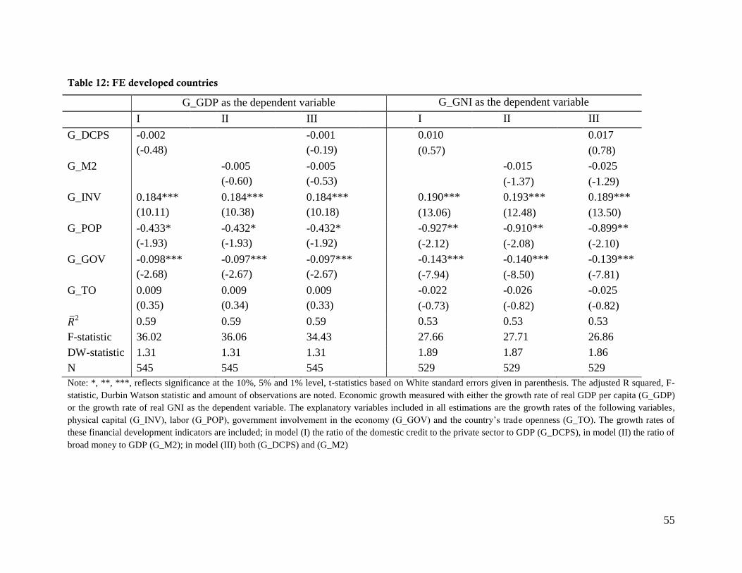
55
Table 12: FE developed countries
G_GDP as the dependent variable G_GNI as the dependent variable
I II III I II III
G_DCPS -0.002
(-0.48)
-0.001
(-0.19)
0.010
(0.57)
0.017
(0.78)
G_M2 -0.005
(-0.60)
-0.005
(-0.53)
-0.015
(-1.37)
-0.025
(-1.29)
G_INV 0.184***
(10.11)
0.184***
(10.38)
0.184***
(10.18)
0.190***
(13.06)
0.193***
(12.48)
0.189***
(13.50)
G_POP -0.433*
(-1.93)
-0.432*
(-1.93)
-0.432*
(-1.92)
-0.927**
(-2.12)
-0.910**
(-2.08)
-0.899**
(-2.10)
G_GOV -0.098***
(-2.68)
-0.097***
(-2.67)
-0.097***
(-2.67)
-0.143***
(-7.94)
-0.140***
(-8.50)
-0.139***
(-7.81)
G_TO 0.009
(0.35)
0.009
(0.34)
0.009
(0.33)
-0.022
(-0.73)
-0.026
(-0.82)
-0.025
(-0.82)
2 0.59 0.59 0.59 0.53 0.53 0.53
F-statistic 36.02 36.06 34.43 27.66 27.71 26.86
DW-statistic 1.31 1.31 1.31 1.89 1.87 1.86
N 545 545 545 529 529 529
Note: *, **, ***, reflects significance at the 10%, 5% and 1% level, t-statistics based on White standard errors given in parenthesis. The adjusted R squared, F-
statistic, Durbin Watson statistic and amount of observations are noted. Economic growth measured with either the growth rate of real GDP per capita (G_GDP)
or the growth rate of real GNI as the dependent variable. The explanatory variables included in all estimations are the growth rates of the following variables,
physical capital (G_INV), labor (G_POP), government involvement in the economy (G_GOV) and the country’s trade openness (G_TO). The growth rates of
these financial development indicators are included; in model (I) the ratio of the domestic credit to the private sector to GDP (G_DCPS), in model (II) the ratio of
broad money to GDP (G_M2); in model (III) both (G_DCPS) and (G_M2)

56
Table 13: FE-IV (1) Developed countries
G_GDP as the dependent variable G_GNI as the dependent variable
I II III I II III
G_DCPS 0.163*
(1.72)
- 0.199
(0.93)
0.098
(1.47)
- 0.096
(0.60)
G_M2 - 0.308
(1.27)
-0.067
(-0.15)
- 0.195
(1.42)
0.038
(0.16)
G_INV 0.158*
(1.83)
0.173*
(1.78)
0.159*
(1.96)
0.226***
(3.56)
0.242***
(5.77)
0.215***
(3.85)
G_POP -0.716
(-1.19)
-1.314
(-1.14)
-0.515
(-0.43)
-1.174*
(-1.75)
-1.493
(-1.54)
-1.294
(-1.63)
G_GOV -0.140
(-0.66)
0.029
(0.14)
-0.127
(-0.51)
-0.085
(-0.40)
-0.010
(-0.05)
-0.079
(-0.35)
G_TO -0.203
(-1.03)
0.035
(0.12)
-0.203
(-0.61)
-0.144
(-0.89)
-0.026
(-0.13)
-0.117
(-0.64)
F-statistic 5.76 5.60 5.51 4.97 5.11 4.82
DW-statistic 1.97 1.87 1.99 2.10 2.11 2.09
N 507 507 507 493 493 493
Note: *, **, ***, reflects significance at the 10%, 5% and 1% level, t-statistics based on White standard errors given in parenthesis. The F-statistic, Durbin
Watson statistic and amount of observations are noted. Economic growth measured either with the growth rate of real GDP per capita (G_GDP) or the growth
rate of real GNI per capita (G_GNI) as the dependent variable. The instrument set used is lagged values of the explanatory variables (-1 to -2). The explanatory
variables in all estimations are the growth rates of the following variables, physical capital (G_INV), labor (G_POP), government’s involvement in the economy
(G_GOV) and the country’s trade openness (G_TO). The growth rates of these financial development indicators are included; in model (I) the ratio of the
domestic credit to the private sector to GDP (G_DCPS), in model (II) the ratio of broad money to GDP (G_M2); in model (III) both (G_DCPS) and (G_M2)
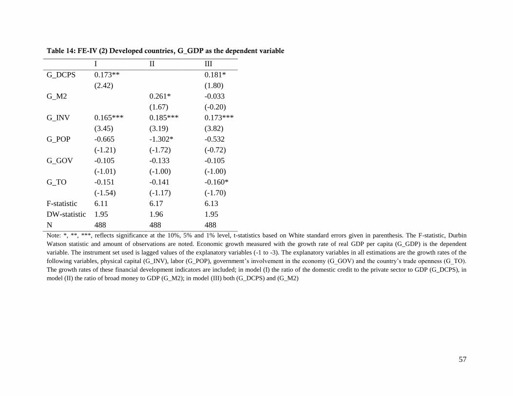
57
Table 14: FE-IV (2) Developed countries, G_GDP as the dependent variable
I II III
G_DCPS 0.173**
(2.42)
0.181*
(1.80)
G_M2 0.261*
(1.67)
-0.033
(-0.20)
G_INV 0.165***
(3.45)
0.185***
(3.19)
0.173***
(3.82)
G_POP -0.665
(-1.21)
-1.302*
(-1.72)
-0.532
(-0.72)
G_GOV -0.105
(-1.01)
-0.133
(-1.00)
-0.105
(-1.00)
G_TO -0.151
(-1.54)
-0.141
(-1.17)
-0.160*
(-1.70)
F-statistic 6.11 6.17 6.13
DW-statistic 1.95 1.96 1.95
N 488 488 488
Note: *, **, ***, reflects significance at the 10%, 5% and 1% level, t-statistics based on White standard errors given in parenthesis. The F-statistic, Durbin
Watson statistic and amount of observations are noted. Economic growth measured with the growth rate of real GDP per capita (G_GDP) is the dependent
variable. The instrument set used is lagged values of the explanatory variables (-1 to -3). The explanatory variables in all estimations are the growth rates of the
following variables, physical capital (G_INV), labor (G_POP), government’s involvement in the economy (G_GOV) and the country’s trade openness (G_TO).
The growth rates of these financial development indicators are included; in model (I) the ratio of the domestic credit to the private sector to GDP (G_DCPS), in
model (II) the ratio of broad money to GDP (G_M2); in model (III) both (G_DCPS) and (G_M2)

58
Table 15: FE-IV (3), G_GDP as the dependent variable
Latin America Developed countries
I II III I II III
G_DCPS 0.156**
(2.20)
- 0.141*
(1.72)
0.110**
(2.58)
0.122
(1.59)
G_M2 0.004
(0.12)
-0.053
(-1.01)
0.115**
(2.12)
-0.015
(-0.16)
G_INV 0.135***
(2.87)
0.129***
(2.98)
0.141***
(3.61)
0.185***
(4.84)
0.206***
(4.96)
0.186***
(5.35)
G_POP -2.137**
(-2.20)
-2.785*
(-1.84)
-2.168**
(-2.20)
-0.443
(-1.02)
-0.658
(-1.33)
-0.375
(-0.87)
G_GOV -0.082
(-1.46)
0.001
(0.01)
-0.022
(-0.41)
-0.078
(-1.20)
-0.078
(-0.93)
-0.074
(-1.09)
G_TO -0.215*
(-1.94)
-0.328***
(-2.82)
-0.217**
(-2.26)
-0.088
(-1.20)
-0.102
(-1.33)
-0.082
(-1.06)
F-statistic 3.70 3.54 3.63 6.13 6.15 6.11
DW-statistic 1.97 1.91 1.92 1.78 1.74 1.80
N 457 464 457 469 469 469
Note: *, **, ***, reflects significance at the 10%, 5% and 1% level, t-statistics based on White standard errors given in parenthesis. The F-statistic, DW-statistic
and amount of observations are noted. Economic growth measured with the growth rate of real GDP per capita (G_GDP) is the dependent variable. The
instrument set used is lagged values of the explanatory variables (-1 to -4). The explanatory variables in all estimations are the growth rates of the following
variables, physical capital (G_INV), labor (G_POP), government involvement in the economy (G_GOV) and the country’s trade openness (G_TO). The growth
rates of these financial development indicators are included; in model (I) the ratio of the domestic credit to the private sector to GDP (G_DCPS), in model (II) the
ratio of broad money to GDP (G_M2); in model (III) both (G_DCPS) and (G_M2)
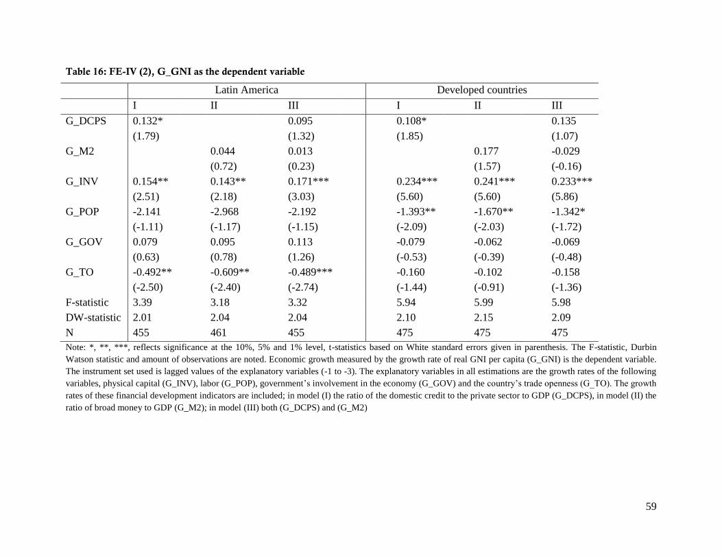
59
Table 16: FE-IV (2), G_GNI as the dependent variable
Latin America Developed countries
I II III I II III
G_DCPS 0.132*
(1.79)
0.095
(1.32)
0.108*
(1.85)
0.135
(1.07)
G_M2 0.044
(0.72)
0.013
(0.23)
0.177
(1.57)
-0.029
(-0.16)
G_INV 0.154**
(2.51)
0.143**
(2.18)
0.171***
(3.03)
0.234***
(5.60)
0.241***
(5.60)
0.233***
(5.86)
G_POP -2.141
(-1.11)
-2.968
(-1.17)
-2.192
(-1.15)
-1.393**
(-2.09)
-1.670**
(-2.03)
-1.342*
(-1.72)
G_GOV 0.079
(0.63)
0.095
(0.78)
0.113
(1.26)
-0.079
(-0.53)
-0.062
(-0.39)
-0.069
(-0.48)
G_TO -0.492**
(-2.50)
-0.609**
(-2.40)
-0.489***
(-2.74)
-0.160
(-1.44)
-0.102
(-0.91)
-0.158
(-1.36)
F-statistic 3.39 3.18 3.32 5.94 5.99 5.98
DW-statistic 2.01 2.04 2.04 2.10 2.15 2.09
N 455 461 455 475 475 475
Note: *, **, ***, reflects significance at the 10%, 5% and 1% level, t-statistics based on White standard errors given in parenthesis. The F-statistic, Durbin
Watson statistic and amount of observations are noted. Economic growth measured by the growth rate of real GNI per capita (G_GNI) is the dependent variable.
The instrument set used is lagged values of the explanatory variables (-1 to -3). The explanatory variables in all estimations are the growth rates of the following
variables, physical capital (G_INV), labor (G_POP), government’s involvement in the economy (G_GOV) and the country’s trade openness (G_TO). The growth
rates of these financial development indicators are included; in model (I) the ratio of the domestic credit to the private sector to GDP (G_DCPS), in model (II) the
ratio of broad money to GDP (G_M2); in model (III) both (G_DCPS) and (G_M2)
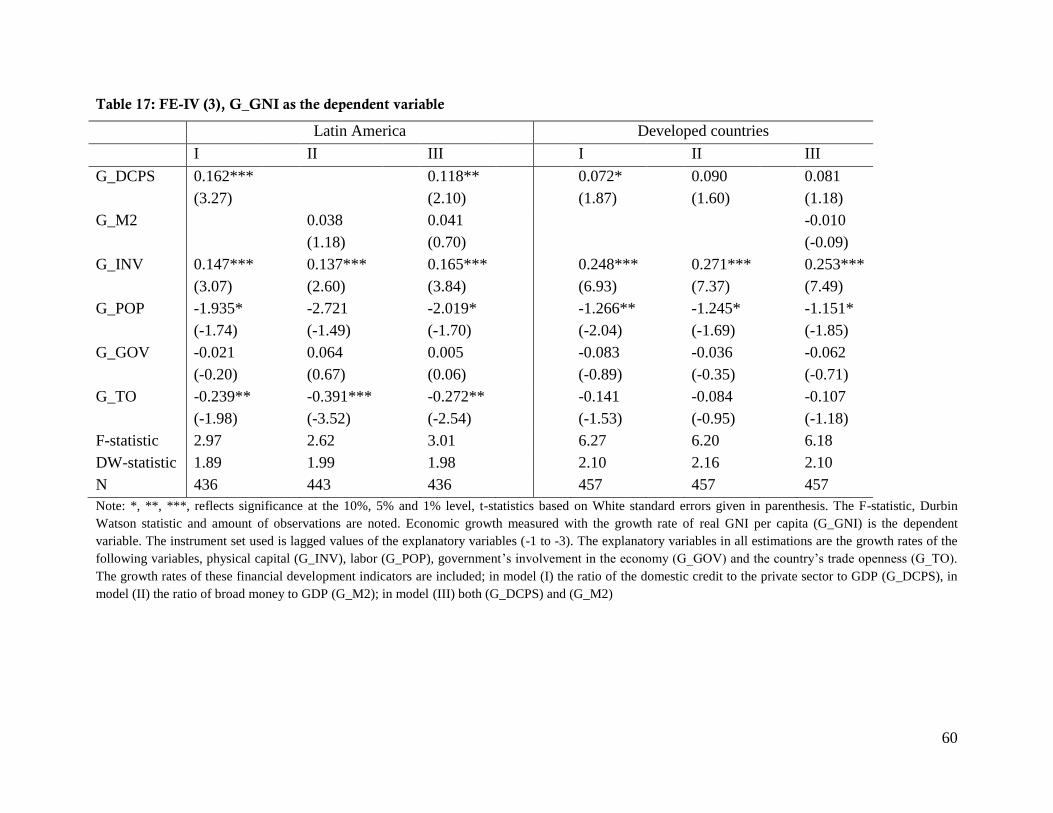
60
Table 17: FE-IV (3), G_GNI as the dependent variable
Latin America Developed countries
I II III I II III
G_DCPS 0.162***
(3.27)
0.118**
(2.10)
0.072*
(1.87)
0.090
(1.60)
0.081
(1.18)
G_M2 0.038
(1.18)
0.041
(0.70)
-0.010
(-0.09)
G_INV 0.147***
(3.07)
0.137***
(2.60)
0.165***
(3.84)
0.248***
(6.93)
0.271***
(7.37)
0.253***
(7.49)
G_POP -1.935*
(-1.74)
-2.721
(-1.49)
-2.019*
(-1.70)
-1.266**
(-2.04)
-1.245*
(-1.69)
-1.151*
(-1.85)
G_GOV -0.021
(-0.20)
0.064
(0.67)
0.005
(0.06)
-0.083
(-0.89)
-0.036
(-0.35)
-0.062
(-0.71)
G_TO -0.239**
(-1.98)
-0.391***
(-3.52)
-0.272**
(-2.54)
-0.141
(-1.53)
-0.084
(-0.95)
-0.107
(-1.18)
F-statistic 2.97 2.62 3.01 6.27 6.20 6.18
DW-statistic 1.89 1.99 1.98 2.10 2.16 2.10
N 436 443 436 457 457 457
Note: *, **, ***, reflects significance at the 10%, 5% and 1% level, t-statistics based on White standard errors given in parenthesis. The F-statistic, Durbin
Watson statistic and amount of observations are noted. Economic growth measured with the growth rate of real GNI per capita (G_GNI) is the dependent
variable. The instrument set used is lagged values of the explanatory variables (-1 to -3). The explanatory variables in all estimations are the growth rates of the
following variables, physical capital (G_INV), labor (G_POP), government’s involvement in the economy (G_GOV) and the country’s trade openness (G_TO).
The growth rates of these financial development indicators are included; in model (I) the ratio of the domestic credit to the private sector to GDP (G_DCPS), in
model (II) the ratio of broad money to GDP (G_M2); in model (III) both (G_DCPS) and (G_M2)