Impact of Removing Covariance Localization in an Ensemble Kalman Filter :Experiments with 10240 Members Using an Intermediate AGCM

KEIICHI KONDO

RIKEN Advanced Institute for Computational Science, Kobe, Japan

TAKEMASA MIYOSHI

RIKEN Advanced Institute for Computational Science, Kobe, Japan, and Department of Atmospheric and Oceanic

Science, University of Maryland, College Park, College Park, Maryland, and Japan Agency for Marine-Earth

Science and Technology, Yokohama, Japan

(Manuscript received 4 November 2015, in final form 7 September 2016)

ABSTRACT

The ensemble Kalman filter (EnKF) with high-dimensional geophysical systems usually employs up to 100

ensemble members and requires covariance localization to reduce the sampling error in the forecast error

covariance between distant locations. The authors’ previous work pioneered implementation of an EnKF

with a large ensemble of up to 10 240 members, but this method required application of a relatively broad

covariance localization to avoid memory overflow. This study modified the EnKF code to save memory and

enabled for the first time the removal of completely covariance localization with an intermediate AGCM.

Using the large sample size, this study aims to investigate the analysis and forecast accuracy, as well as the

impact of covariance localization when the sampling error is small. A series of 60-day data assimilation cycle

experiments with different localization scales are performed under the perfect model scenario to investigate

the pure impact of covariance localization. The results show that the analysis and 7-day forecasts are much

improved by removing covariance localization and that the long-range covariance between distant locations

plays a key role. The eigenvectors of the background error covariance matrix based on the 10 240 ensemble

members are explicitly computed and reveal long-range structures.

1. Introduction

The ensemble Kalman filter (EnKF; Evensen 1994) is

an advanced data assimilation method and approxi-

mates the Kalman filter (KF; Kalman 1960) by esti-

mating the forecast error covariance from a limited

number of samples or ensemble forecasts. In recent

EnKF studies using atmospheric models, the ensemble

size was usually limited to about 100 to balance the ac-

curacy of the EnKF and the model’s computational

complexity such as its resolution and physics schemes.

The limited ensemble size causes spurious sam-

pling errors, which contaminate the estimates of the

background error covariance and degrade the analysis

accuracy. Therefore, covariance localization plays an

essential role in limiting the influence of the observa-

tions within a prescribed distance and reduces the im-

pact of spurious sampling errors between distant

locations (e.g., Houtekamer and Mitchell 1998; Hamill

et al. 2001). The choice of the localization functional

shape is a tuning parameter, and this study employs two

types: the step function, which becomes zero at a certain

distance, and the Gaussian function, which is forced to

be zero at and beyond a distance of 2(10/3)1/2 standard

deviations (or simply SD hereafter) from the center of

localization. If we fit the Gaussian function to the widely

used Gaspari–Cohn function with compact support

(Gaspari and Cohn 1999), the Gaspari–Cohn function

becomes zero at this distance. In this study, the locali-

zation scale is defined as the distance at which the lo-

calization function becomes zero (i.e., the radius of

influence). Although optimal localization was explored

theoretically (Perianez et al. 2014; Flowerdew 2015;

Corresponding author address: Keiichi Kondo, RIKEN Ad-

vanced Institute for Computational Science, 7-1-26 Minatojima-

minami-machi, Chuo-ku, Kobe, Hyogo, 650-0047, Japan.

E-mail: keiichi.kondo@riken.jp

Denotes Open Access content.

DECEMBER 2016 KONDO AND M IYO SH I 4849

DOI: 10.1175/MWR-D-15-0388.1

� 2016 American Meteorological SocietyUnauthenticated | Downloaded 02/15/22 05:21 AM UTC

Ménétrier et al. 2015a,b), previous studies chose the lo-

calization scale primarily based on the ensemble size and

model resolution (Table 1). Higher-resolution models

resolve smaller-scale phenomena and generally require a

shorter localization scale. If the ensemble size is smaller,

the localization scale also becomes shorter to avoid the

deleterious influence of the sampling errors. Such narrow

localization may limit exceedingly the number of obser-

vations assimilated at each grid point for high-resolution

models. To increase the effective local number of ob-

servations, multiscale localization methods have been

explored (Zhang et al. 2009; Rainwater and Hunt 2013;

Miyoshi and Kondo 2013; Kondo et al. 2013).

Miyoshi et al. (2014, hereafter MKI14) increased the

ensemble size up to 10240, two orders of magnitude

greater than the typical choice of about 100, and in-

vestigated long-range error-correlation structures with an

intermediate AGCM known as the Simplified Parame-

terizations, Primitive Equation Dynamics (SPEEDY)

model (Molteni 2003) using the local ensemble transform

Kalman filter (LETKF; Hunt et al. 2007). More recently,

Miyoshi et al. (2015) ran a similar 10 240-member

LETKF experiment for the real atmosphere using the

Nonhydrostatic Icosahedral AtmosphericModel (NICAM;

Satoh et al. 2008, 2014) and real-world observations. MKI14

ran a 3-week experiment involving the 10 240-member

SPEEDY–LETKF with 7303-km Gaussian-function

horizontal localization (SD 5 2000 km) and found that

the horizontal correlation structures extended at conti-

nental or even planetary scales. It is still an open ques-

tion as to what would be the impact of the long-range

error correlations on data assimilation. Although

with 10 240 members it may be better to remove

localization, a larger ensemble demands a larger mem-

ory space. Running a 10 240-member LETKF without

localization caused memory overflow in MKI14’s ex-

periments. Therefore, MKI14 had to apply relatively

broad 7303-km Gaussian-function localization, which is

the maximum localization scale in MKI14’s environ-

ment, to avoid memory overflow.

In this study, we improve the LETKF code of MKI14

and save memory, so that we can remove covariance lo-

calization completely with 10240 members. We aim to

compare the accuracy of the analysis and subsequent

7-day forecasts by investigating sensitivities to the en-

semble size from 20 to 10240 and to different localization

settings using the Gaussian function and the local patch

(Ott et al. 2004) provided by the step function. To the best

of the authors’ knowledge, the experiments will reveal for

the first time the impact of continental- to planetary-scale

error correlations on the analysis and forecast. Such long-

range error correlations have not been considered ex-

plicitly in meteorological data assimilations thus far.

Section 2 describes the LETKF system with the

SPEEDY model. Section 3 describes the experimental

design, and section 4 presents the results with along with

some discussion. In section 5 we perform explicit ei-

genvalue decomposition of the forecast error covariance

matrix estimated by 10 240 ensemble members. Finally,

section 6 provides our conclusions.

2. SPEEDY–LETKF system

The SPEEDY model is an intermediate atmospheric

general circulation model with the primitive equations

dynamical core, and the T30–L7 resolution corresponds

TABLE 1. Combinations of the ensemble size, model resolution,

and localization scale from previous studies.

Ensemble

size Resolution

Localization

scale (km)

Kondo and Tanaka

(2009)

40 224 km 1826

Zhang et al. (2009) 30 40.5 km 1215

13.5 km 405

4.5 km 135

Miyoshi et al. (2010) 50 TL159/L40 1461

Yussouf and Stensrud

(2010)

40 1 km 4

Miyoshi and Kunii

(2012)

20 60 km 1461

Miyoshi and Kondo

(2013)

20 T30L7 2556

Kondo et al. (2013)

Kunii (2014) 50 15 km 730

5 km 365

Terasaki et al. (2015) 20 112 km 1461

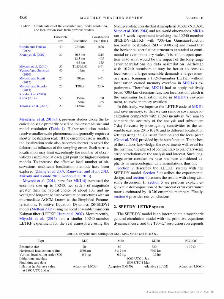
TABLE 2. Experimental settings for M20, M80, M320, and NOLOC.

Expt M20 M80 M320 NOLOC

Ensemble size 20 80 320 10 240

Horizontal localization radius 2556 km 5112 km 7303 km —

Vertical localization scale (SD) 0.1 lnp 0.2 lnp 0.3 lnp —

Initial time and date 0000 UTC 1 Jan

Final time and date 1800 UTC 1 Mar

Inflation (global avg value

at 1800 UTC 1 Mar)

Adaptive (1.0659) Adaptive (1.0670) Adaptive (1.0102) Adaptive (1.0060)

4850 MONTHLY WEATHER REV IEW VOLUME 144

Unauthenticated | Downloaded 02/15/22 05:21 AM UTC

to 963 48 grid points horizontally and 7 levels vertically,

totaling 133 632 prognostic variables. The SPEEDY

model has been used in a number of studies on data

assimilation (e.g., Miyoshi 2005; Greybush et al. 2011;

Miyoshi 2011; Miyoshi and Kondo 2013; Kondo et al.

2013). The SPEEDY model has simplified forms of

physical parameterization schemes such as large-scale

condensation, convection, clouds, short- and longwave

radiation, surface fluxes and vertical diffusion.

Hunt et al. (2007) proposed the LETKF by applying

the ensemble transform Kalman filter (ETKF; Bishop

et al. 2001) algorithm to the local ensemble Kalman

filter (LEKF; Ott et al. 2004). Let X denote an n 3 m

matrix, where n andm denote the system dimension and

ensemble size, respectively, so that each column corre-

sponds to amodel state vector. Them3m analysis error

covariance matrix ~Pa in the ensemble space is written as

~Pa 5 [(m2 1)I /r1 (HdXf )TR21(HdXf )]21

5UD21UT , (1)

[cf. Eqs. (3) and (9) in Miyoshi and Yamane (2007)].

Here, r denotes the covariance inflation factor, and

H,dXf , and R denote the linear observation operator,

background ensemble perturbations, and observation

error covariance matrix, respectively. To solve the ma-

trix inversion of Eq. (1), the LETKF computes the ei-

genvalue decomposition. In addition, U is composed of

the eigenvectors, so thatUUT 5 I. The diagonal matrixD

is composed of the eigenvalues. The ensemble analysis

Xa is obtained from

Xa 5 x f11 dXf [(~Pa)21(HdXf )TR21(yo 2Hx f )1

1ffiffiffiffiffiffiffiffiffiffiffiffiffi

m2 1p

(~Pa)21/2] , (2)

[cf. Eqs. (6) and (7) in Miyoshi and Yamane (2007)].

Here, x f and yo denote the background ensemble mean

and observations, respectively. Here, 1 denotes an

m-dimensional row vector with all elements being 1.

Using the eigenvalue decomposition [Eq. (1)], Eq. (2) is

solved efficiently. The LETKF computes Eqs. (1) and

(2) at every grid point independently, so that the

LETKF can compute Xa efficiently in parallel. In

fact, Miyoshi and Yamane (2007) showed that the paral-

lelization ratio reached 99.99% using up to 240 nodes on

the Japanese Earth Simulator supercomputer.

MKI14 ran a 3-week-long 10240-member SPEEDY–

LETKFexperimentwith a 7303-km localization scale (i.e.,

the Gaussian localization function with SD 5 2000km),

using 4608 nodes of the Japanese flagship K computer.

The K computer has 88 128 nodes with its peak perfor-

mance of 10 petaflops, which ranked number 5 in the

top-500 list as of June 2016 (http://www.top500.org/lists/

2016/06/). As already mentioned in the introduction,

although MKI14 had to apply localization to avoid

memory overflow, in this study the SPEEDY–LETKF

code of MKI14 was improved, so that we could avoid

memory overflow even without localization at all.

3. Experimental settings

The experiments in this study assume the perfect

model following MKI14. The nature run is initialized at

0000 UTC 1 January by the standard atmosphere at rest

(i.e., no wind), and the first year is considered to be a

spinup period. The experimental period is 60 days from

0000 UTC 1 January in the second year of the nature

run. The observational error standard deviations are

fixed to 1.0m s21, 1.0K, 0.1 g kg21, and 1.0 hPa for hor-

izontal wind components, temperature, specific humid-

ity, and surface pressure, respectively. The observations

are simulated by adding independent Gaussian random

numbers to the nature run every 6h at the radiosonde-

like locations (cf. section 4; Fig. 5, cross marks) for all

seven vertical levels, but the observations of specific

humidity are simulated from the bottom to the fourth

model level (about 500 hPa). The number of observa-

tions is 10 816 every 6 h, which is very similar to the

ensemble size of 10 240. Six-hourly data assimilation

cycles are performed.

First, the NOLOC experiment, standing for no local-

ization, is performed using 10 240 ensemble members

without localization at all, either in the horizontal or in

the vertical. NOLOC is equivalent to the global ETKF

theoretically, and an ETKF implementation may be

much more efficient than the LETKF option. However,

for a pure comparison, we use the same LETKF code

with different localization settings even for NOLOC. To

investigate the performance of NOLOC, three addi-

tional experiments are performed with 20, 80, and

320 members, which are often used experimentally or

operationally, and they are called M20, M80, and M320,

respectively (Table 2). The horizontal localization scales

of M20 and M80 with the Gaussian function are manu-

ally tuned to be 2556 and 5112km (SD 5 700 and

1400km), respectively. The localization scale of M320 is

fixed at 7303km (SD5 2000km) following MKI14. The

vertical localization scales for M20, M80, and M320 are

chosen to be SD 5 0.1, 0.2, and 0.3 in the natural loga-

rithm of the pressure coordinate for the Gaussian

function, respectively. Applying the tight vertical lo-

calization is essential for M20, as was the case in the

previous studies using the SPEEDY–LETKF system

(e.g., Miyoshi 2005, 2011; Kang et al. 2012). These ex-

periments are initialized at 0000 UTC 1 January by the

DECEMBER 2016 KONDO AND M IYO SH I 4851

Unauthenticated | Downloaded 02/15/22 05:21 AM UTC

initial ensemble states randomly chosen from the long-

term nature runs in December and January after De-

cember of the ninth year. For all experiments, the

adaptive covariance inflation method of Miyoshi (2011)

is applied.

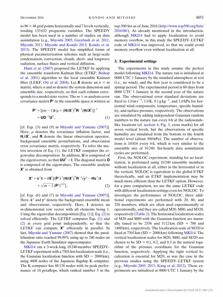
Next, to investigate the sensitivity to the ensemble size

while fixing the localization, we ran five experiments with

80, 320, 1280, 5120, and 10240 members with 7303-km

(SD 5 2000km) Gaussian localization horizontally but

without vertical localization (Table 3). The experiment

with 10 240 members is called LG7, which stands for

localization, Gaussian, and the radius of 7303km; the

other experiments are named simply for their ensemble

sizes: 80, 320, 1280, and 5120. These experiments

are initialized with the first guess of NOLOC at

0000 UTC 24 January, and run for 37 days until the end

of the experiment period. More precisely, the initial

ensemble perturbations are chosen from NOLOC, and

the initial ensemble mean of each experiment is the

same as that of NOLOC.

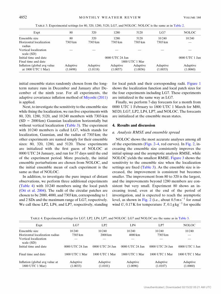
In addition, to investigate the pure impact of distant

observations, we perform three additional experiments

(Table 4) with 10 240 members using the local patch

(Ott et al. 2004). The radii of the circular patches are

chosen to be 2000, 4000, and 7303km, corresponding to 1

and 2 SDs and the maximum range of LG7, respectively.

We call these LP2, LP4, and LP7, respectively, standing

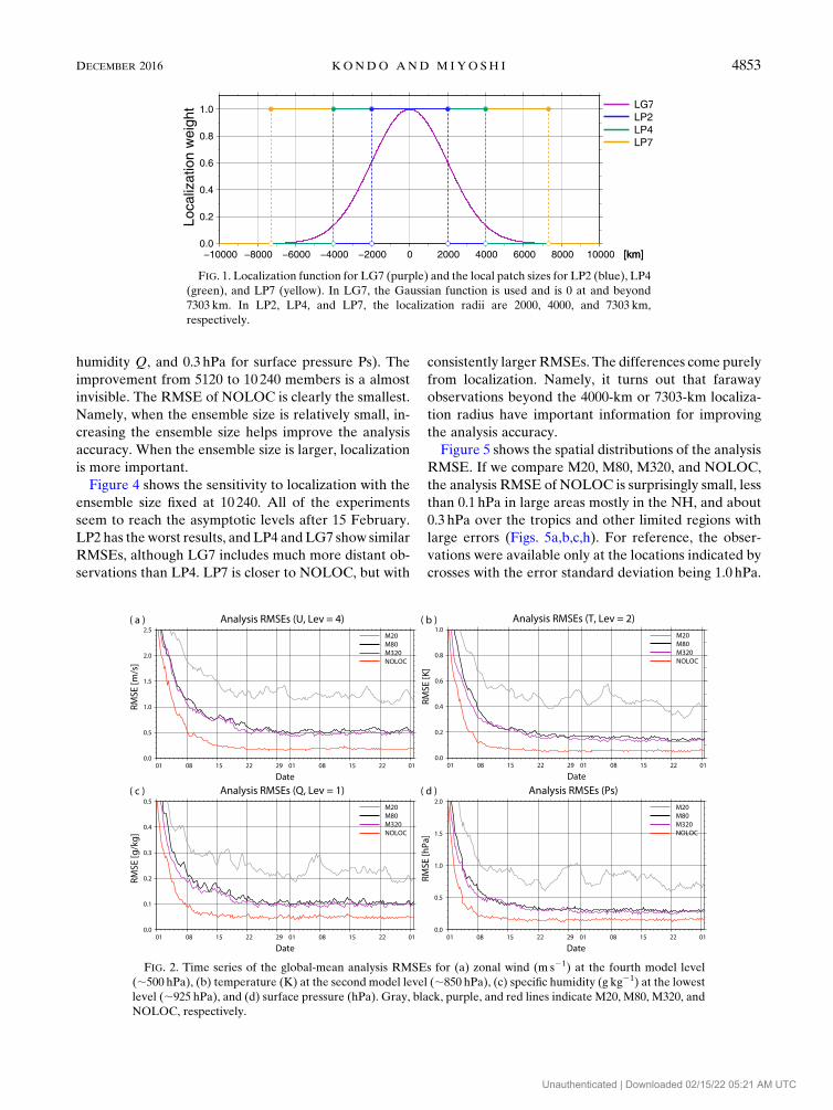
for local patch and their corresponding radii. Figure 1

shows the localization function and local patch sizes for

the four experiments including LG7. These experiments

are initialized in the same way as LG7.

Finally, we perform 7-day forecasts for a month from

0000 UTC 1 February to 1800 UTC 1 March for M80,

M320, LG7, LP2, LP4, LP7, and NOLOC. The forecasts

are initialized at the ensemble mean states.

4. Results and discussion

a. Analysis RMSE and ensemble spread

NOLOC shows the most accurate analyses among all

of the experiments (Figs. 2–4, red curves). In Fig. 2, in-

creasing the ensemble size consistently improves the

initial spinup and the asymptotic analysis RMSE, while

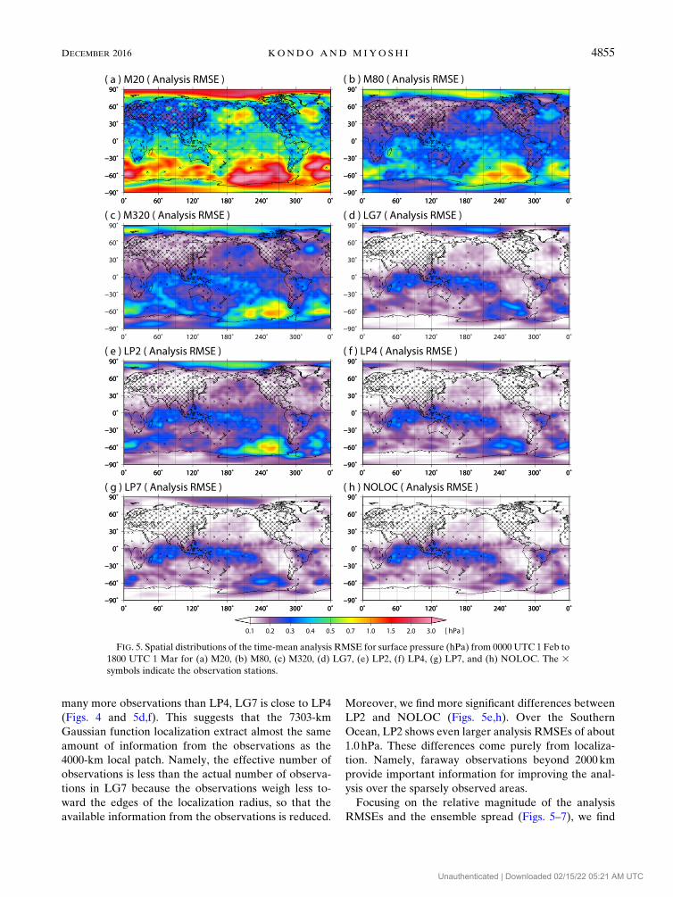
NOLOC yields the smallest RMSE. Figure 3 shows the

sensitivity to the ensemble size when the localization

settings are fixed (Table 3). As the ensemble size is in-

creased, the improvement is consistent but becomes

smaller. The improvement from 80 to 320 is the largest,

and the improvements beyond 1280 members are con-

sistent but very small. Experiment 80 shows an in-

creasing trend, even at the end of the period of

investigation, and is expected to reach the asymptotic

level, as shown in Fig. 2 (i.e., about 0.5m s21 for zonal

wind U, 0.17K for temperature T, 0.1 g kg21 for specific

TABLE 3. Experimental settings for 80, 320, 1280, 5120, LG7, and NOLOC. NOLOC is the same as in Table 2.

Expt 80 320 1280 5120 LG7 NOLOC

Ensemble size 80 320 1280 5120 10 240 10 240

Horizontal localization

radius

7303 km 7303 km 7303 km 7303 km 7303 km —

Vertical localization

scale (SD)

— — — — — —

Initial time and date 0000 UTC 24 Jan 0000 UTC 1 Jan

Final time and date 1800 UTC 1 Mar

Inflation (global avg value

at 1800 UTC 1 Mar)

Adaptive

(1.0498)

Adaptive

(1.0118)

Adaptive

(1.0057)

Adaptive

(1.0036)

Adaptive

(1.0033)

Adaptive

(1.0060)

TABLE 4. Experimental settings for LG7, LP2, LP4, LP7, and NOLOC. LG7 and NOLOC are the same as in Table 3.

Expt LG7 LP2 LP4 LP7 NOLOC

Ensemble size 10 240 10 240 10 240 10 240 10 240

Horizontal localization radius 7303 km 2000 km 4000 km 7303 km —

Vertical localization

scale (SD)

— — — — —

Initial time and date 0000 UTC 24 Jan 0000 UTC 24 Jan 0000 UTC 24 Jan 0000 UTC 24 Jan 0000 UTC 1 Jan

Final time and date 1800 UTC 1 Mar 1800 UTC 1 Mar 1800 UTC 1 Mar 1800 UTC 1 Mar 1800 UTC 1 Mar

Inflation (global avg value at

1800 UTC 1 Mar)

Adaptive

(1.0033)

Adaptive

(1.0101)

Adaptive

(1.0096)

Adaptive

(1.0107)

Adaptive

(1.0060)

4852 MONTHLY WEATHER REV IEW VOLUME 144

Unauthenticated | Downloaded 02/15/22 05:21 AM UTC

humidity Q, and 0.3 hPa for surface pressure Ps). The

improvement from 5120 to 10 240 members is a almost

invisible. The RMSE of NOLOC is clearly the smallest.

Namely, when the ensemble size is relatively small, in-

creasing the ensemble size helps improve the analysis

accuracy. When the ensemble size is larger, localization

is more important.

Figure 4 shows the sensitivity to localization with the

ensemble size fixed at 10 240. All of the experiments

seem to reach the asymptotic levels after 15 February.

LP2 has the worst results, and LP4 andLG7 show similar

RMSEs, although LG7 includes much more distant ob-

servations than LP4. LP7 is closer to NOLOC, but with

consistently larger RMSEs. The differences come purely

from localization. Namely, it turns out that faraway

observations beyond the 4000-km or 7303-km localiza-

tion radius have important information for improving

the analysis accuracy.

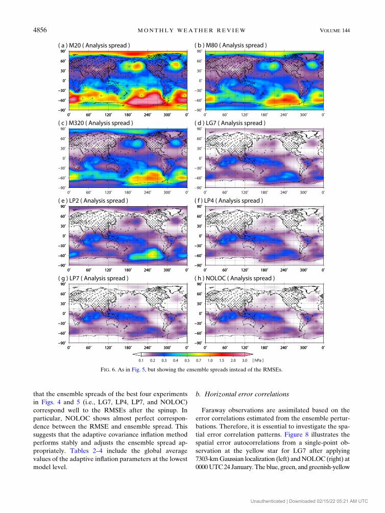
Figure 5 shows the spatial distributions of the analysis

RMSE. If we compare M20, M80, M320, and NOLOC,

the analysis RMSE of NOLOC is surprisingly small, less

than 0.1 hPa in large areas mostly in the NH, and about

0.3 hPa over the tropics and other limited regions with

large errors (Figs. 5a,b,c,h). For reference, the obser-

vations were available only at the locations indicated by

crosses with the error standard deviation being 1.0 hPa.

FIG. 1. Localization function for LG7 (purple) and the local patch sizes for LP2 (blue), LP4

(green), and LP7 (yellow). In LG7, the Gaussian function is used and is 0 at and beyond

7303 km. In LP2, LP4, and LP7, the localization radii are 2000, 4000, and 7303 km,

respectively.

FIG. 2. Time series of the global-mean analysis RMSEs for (a) zonal wind (m s21) at the fourth model level

(;500 hPa), (b) temperature (K) at the second model level (;850 hPa), (c) specific humidity (g kg21) at the lowest

level (;925 hPa), and (d) surface pressure (hPa). Gray, black, purple, and red lines indicate M20, M80, M320, and

NOLOC, respectively.

DECEMBER 2016 KONDO AND M IYO SH I 4853

Unauthenticated | Downloaded 02/15/22 05:21 AM UTC

We find that the error in the extratropics is reduced

significantly by increasing the ensemble size, but in the

tropics, the error reduction is not as effective.

The analysis RMSEs for LG7, LP4, LP7, andNOLOC

are very similar to each other (Figs. 5d,f,g,h). However,

over the Southern Ocean, especially around 2208–2608longitude, where the observations are sparse, LG7, LP4,

and LP7 show analysis RMSEs reaching about 0.4 hPa,

larger than about 0.3 hPa found for NOLOC. Although

LG7 has a localization radius of 7303km and includes

FIG. 3. As in Fig. 2, but after 21 January for the experiments with different ensemble sizes—80 (black), 320

(purple), 1280 (blue), 5120 (greenish-yellow), LG7 (pink), and NOLOC (red)—with localization settings fixed. The

experiments were initialized on 24 Janwith subsets of 10 240 ensemble perturbations of NOLOC recentered around

the ensemble mean of NOLOC.

FIG. 4. As in Fig. 3, but for the experiments with different localization settings—LG7 (pink), LP2 (blue), LP4

(green), LP7 (greenish-yellow), and NOLOC (red)–and with the ensemble size fixed at 10 240.

4854 MONTHLY WEATHER REV IEW VOLUME 144

Unauthenticated | Downloaded 02/15/22 05:21 AM UTC

many more observations than LP4, LG7 is close to LP4

(Figs. 4 and 5d,f). This suggests that the 7303-km

Gaussian function localization extract almost the same

amount of information from the observations as the

4000-km local patch. Namely, the effective number of

observations is less than the actual number of observa-

tions in LG7 because the observations weigh less to-

ward the edges of the localization radius, so that the

available information from the observations is reduced.

Moreover, we find more significant differences between

LP2 and NOLOC (Figs. 5e,h). Over the Southern

Ocean, LP2 shows even larger analysis RMSEs of about

1.0 hPa. These differences come purely from localiza-

tion. Namely, faraway observations beyond 2000km

provide important information for improving the anal-

ysis over the sparsely observed areas.

Focusing on the relative magnitude of the analysis

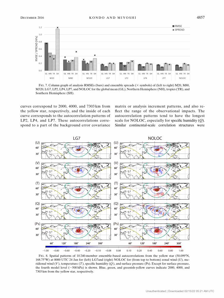
RMSEs and the ensemble spread (Figs. 5–7), we find

FIG. 5. Spatial distributions of the time-mean analysis RMSE for surface pressure (hPa) from 0000 UTC 1 Feb to

1800 UTC 1 Mar for (a) M20, (b) M80, (c) M320, (d) LG7, (e) LP2, (f) LP4, (g) LP7, and (h) NOLOC. The 3symbols indicate the observation stations.

DECEMBER 2016 KONDO AND M IYO SH I 4855

Unauthenticated | Downloaded 02/15/22 05:21 AM UTC

that the ensemble spreads of the best four experiments

in Figs. 4 and 5 (i.e., LG7, LP4, LP7, and NOLOC)

correspond well to the RMSEs after the spinup. In

particular, NOLOC shows almost perfect correspon-

dence between the RMSE and ensemble spread. This

suggests that the adaptive covariance inflation method

performs stably and adjusts the ensemble spread ap-

propriately. Tables 2–4 include the global average

values of the adaptive inflation parameters at the lowest

model level.

b. Horizontal error correlations

Faraway observations are assimilated based on the

error correlations estimated from the ensemble pertur-

bations. Therefore, it is essential to investigate the spa-

tial error correlation patterns. Figure 8 illustrates the

spatial error autocorrelations from a single-point ob-

servation at the yellow star for LG7 after applying

7303-kmGaussian localization (left) andNOLOC (right) at

0000UTC24 January. The blue, green, and greenish-yellow

FIG. 6. As in Fig. 5, but showing the ensemble spreads instead of the RMSEs.

4856 MONTHLY WEATHER REV IEW VOLUME 144

Unauthenticated | Downloaded 02/15/22 05:21 AM UTC

curves correspond to 2000, 4000, and 7303 km from

the yellow star, respectively, and the inside of each

curve corresponds to the autocorrelation patterns of

LP2, LP4, and LP7. These autocorrelations corre-

spond to a part of the background error covariance

matrix or analysis increment patterns, and also re-

flect the range of the observational impacts. The

autocorrelation patterns tend to have the longest

scale for NOLOC, especially for specific humidity (Q).

Similar continental-scale correlation structures were

FIG. 7. Column graph of analysis RMSEs (bars) and ensemble spreads (3 symbols) of (left to right) M20, M80,

M320, LG7, LP2, LP4, LP7, andNOLOC for the global mean (GL), NorthernHemisphere (NH), tropics (TR), and

Southern Hemisphere (SH).

FIG. 8. Spatial patterns of 10 240-member ensemble-based autocorrelations from the yellow star (50.0998N,

168.758W) at 0000 UTC 24 Jan for (left) LG7and (right) NOLOC for (from top to bottom) zonal wind (U), me-

ridional wind (V ), temperature (T ), specific humidity (Q ), and surface pressure (Ps). Except for surface pressure,

the fourth model level (;500 hPa) is shown. Blue, green, and greenish-yellow curves indicate 2000, 4000, and

7303 km from the yellow star, respectively.

DECEMBER 2016 KONDO AND M IYO SH I 4857

Unauthenticated | Downloaded 02/15/22 05:21 AM UTC

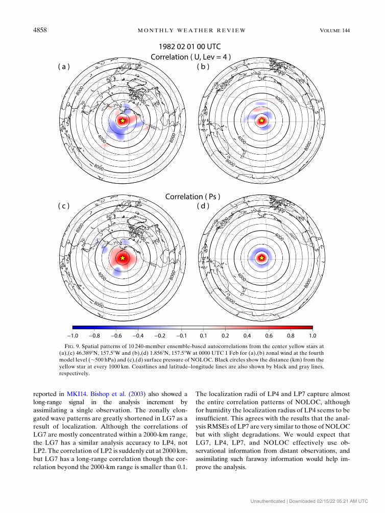
reported in MKI14. Bishop et al. (2003) also showed a

long-range signal in the analysis increment by

assimilating a single observation. The zonally elon-

gated wave patterns are greatly shortened in LG7 as a

result of localization. Although the correlations of

LG7 are mostly concentrated within a 2000-km range,

the LG7 has a similar analysis accuracy to LP4, not

LP2. The correlation of LP2 is suddenly cut at 2000 km,

but LG7 has a long-range correlation though the cor-

relation beyond the 2000-km range is smaller than 0.1.

The localization radii of LP4 and LP7 capture almost

the entire correlation patterns of NOLOC, although

for humidity the localization radius of LP4 seems to be

insufficient. This agrees with the results that the anal-

ysis RMSEs of LP7 are very similar to those of NOLOC

but with slight degradations. We would expect that

LG7, LP4, LP7, and NOLOC effectively use ob-

servational information from distant observations, and

assimilating such faraway information would help im-

prove the analysis.

FIG. 9. Spatial patterns of 10 240-member ensemble-based autocorrelations from the center yellow stars at

(a),(c) 46.3898N, 157.58W and (b),(d) 1.8568N, 157.58W at 0000 UTC 1 Feb for (a),(b) zonal wind at the fourth

model level (;500 hPa) and (c),(d) surface pressure of NOLOC. Black circles show the distance (km) from the

yellow star at every 1000 km. Coastlines and latitude–longitude lines are also shown by black and gray lines,

respectively.

4858 MONTHLY WEATHER REV IEW VOLUME 144

Unauthenticated | Downloaded 02/15/22 05:21 AM UTC

We further investigate the correlation length scales in

different regions. When the ensemble size is small, the

peaks of the analysis RMSEs . 1.0hPa are located over

the sparsely observed areas (Figs. 5a–c). By contrast,

NOLOC shows the peaks of the analysis RMSEs ;0.3hPa mainly over the tropics (Fig. 5h). The analysis

RMSEs of the tropics are relatively similar in all of the

experiments (Fig. 5). Hence, we may hypothesize that the

tropics tend to have narrower correlations, and that it is

harder to improve the results by assimilating faraway ob-

servations. Figure 9 shows the autocorrelations similar to

Fig. 8, but from two different points in the extratropics and

tropics. The correlation structures over the extratropics are

widely spread, and the correlations reach 4000km in cer-

tain directions. By contrast, the correlations over the

tropics stay mostly within 3000 (2000)km for the zonal

wind (surface pressure).On average, the extratropics show

clearly longer-range correlations than do the tropics

(Fig. 10). The slight improvements over the tropics may be

related to the convectively dominated tropical dynamics,

so that the correlation ranges tend to be shorter.

c. Analysis increments

To investigate how data assimilation with and without

localization reduces the actual error, we focus on the dif-

ferences in the analysis increments. The analysis in-

crements are the corrections made to the first guess to

obtain the analysis. Figure 11 shows the analysis in-

crements for themeridional wind at 0000UTC 24 January.

Here, the 80- and 320-member ensemble perturbations

FIG. 10. As in Fig. 8, but averaged for a month from 0000 UTC 1 Feb to 1800 UTC 1 Mar.

DECEMBER 2016 KONDO AND M IYO SH I 4859

Unauthenticated | Downloaded 02/15/22 05:21 AM UTC

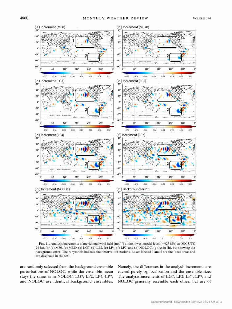
are randomly selected from the background ensemble

perturbations of NOLOC, while the ensemble mean

stays the same as in NOLOC. LG7, LP2, LP4, LP7,

and NOLOC use identical background ensembles.

Namely, the differences in the analysis increments are

caused purely by localization and the ensemble size.

The analysis increments of LG7, LP2, LP4, LP7, and

NOLOC generally resemble each other, but are of

FIG. 11. Analysis increments of meridional wind field (m s21) at the lowest model level (;925 hPa) at 0000 UTC

24 Jan for (a) M80, (b) M320, (c) LG7, (d) LP2, (e) LP4, (f) LP7, and (h) NOLOC. (g) As in (h), but showing the

background error. The 3 symbols indicate the observation stations. Boxes labeled 1 and 2 are the focus areas and

are discussed in the text.

4860 MONTHLY WEATHER REV IEW VOLUME 144

Unauthenticated | Downloaded 02/15/22 05:21 AM UTC

different magnitudes (Figs. 11c–g). By contrast, 80 and 320

members have generally much smaller analysis increments

(Figs. 11a,b).We focus on the areas surrounded by boxes 1

and 2, where we find relatively large analysis increments.

All 10240-member experiments capture the zonal wave

pattern in area 1, which reduces the background error

(Fig. 11h). The wave patterns are stronger in LG7, LP4,

LP7, and NOLOC, and weaker in LP2. LP2 misses the

signal over the western part of area 1 (Fig. 11d). Similar

discussions can be applied to area 2. In the western part

of area 2, LP2 does not create anything. As a result,

relatively large analysis errors remain in LP2. By con-

trast, LG7, LP4, LP7, and NOLOC create large ampli-

tudes of the analysis increments, although the analysis

increment of LG7 is relatively weak. Therefore, longer-

range localization has a large impact across the sparsely

observed areas by assimilating faraway observations,

whereas even if the localization radius is long, as in LG7,

the Gaussian function localization reduces the obser-

vation impact. Namely, Fig. 11 suggests that the amount

of observation information for LG7 be lower than for

LP4, although the Gaussian function localization with

SD 5 2000 km has the same range as LP7.

d. Forecast RMSE

It is important to investigate if the improvement

in the analysis persists in the medium-range forecasts.

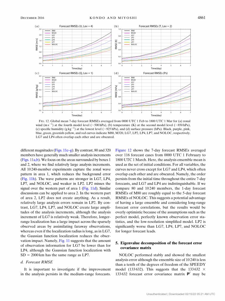
Figure 12 shows the 7-day forecast RMSEs averaged

over 116 forecast cases from 0000 UTC 1 February to

1800 UTC 1March. Here, the analysis ensemble mean is

used as the set of initial conditions. For all variables, the

curves never cross except for LG7 and LP4, which often

overlap each other and are obscured. Namely, the order

persists from the initial time throughout the entire 7-day

forecasts, and LG7 and LP4 are indistinguishable. If we

compare 80 and 10 240 members, the 1-day forecast

RMSEs of M80 are roughly equal to the 5-day forecast

RMSEs of NOLOC. This suggests a potential advantage

of having a large ensemble and considering long-range

forecast error correlations, but the results would be

overly optimistic because of the assumptions such as the

perfect model, perfectly known observation error sta-

tistics, and the low-resolution simplified model. LP2 is

significantly worse than LG7, LP4, LP7, and NOLOC

for longer forecast leads.

5. Eigenvalue decomposition of the forecast errorcovariance matrix

NOLOC performed stably and showed the smallest

analysis error although the ensemble size of 10 240 is less

than a tenth of the degrees of freedom of the SPEEDY

model (133 632). This suggests that the 133 632 3133 632 forecast error covariance matrix Pf may be

FIG. 12. Global mean 7-day forecast RMSEs averaged from 0000 UTC 1 Feb to 1800 UTC 1 Mar for (a) zonal

wind (m s21) at the fourth model level (;500 hPa), (b) temperature (K) at the second model level (;850 hPa),

(c) specific humidity (g kg21) at the lowest level (;925 hPa), and (d) surface pressure (hPa). Black, purple, pink,

blue, green, greenish-yellow, and red curves indicate M80, M320, LG7, LP2, LP4, LP7, and NOLOC, respectively.

LG7 and LP4 often overlap each other and are obscured.

DECEMBER 2016 KONDO AND M IYO SH I 4861

Unauthenticated | Downloaded 02/15/22 05:21 AM UTC

estimated accurately from the 10 240-member ensemble.

Usually, it is difficult to compute the explicit eigenvalue

decomposition of Pf mainly because of the large

dimensionality of Pf . Here, we take advantage of

the K computer and attempt to compute the eigenvalue

decomposition of the 133 632 3 133 632 covariance

matrix explicitly.

Using the efficient eigenvalue decomposition soft-

ware EigenExa (Imamura et al. 2011), MKI14 re-

ported the acceleration of the computations of the

10240-member LETKF by a factor of 8. Here, we take

advantage of EigenExa and solve the eigenvalue

decomposition ofP f. EigenExa is appliedwith 2304 nodes

on the K computer, and the eigenvalues and eigenvectors

of P f are obtained within about 3min. As a preprocess of

the eigenvalue decomposition, the variables are normal-

ized to have equal weights. Namely, the latitude-weighted

dX f is calculated by multiplying by(cosl)1/2, where l de-

notes the latitude. In addition, the latitude-weighted dX f

is normalized by the standard deviation of each variable

and at every vertical level. When we plot eigenvectors in

the horizontal, we divide by (cosl)1/2.

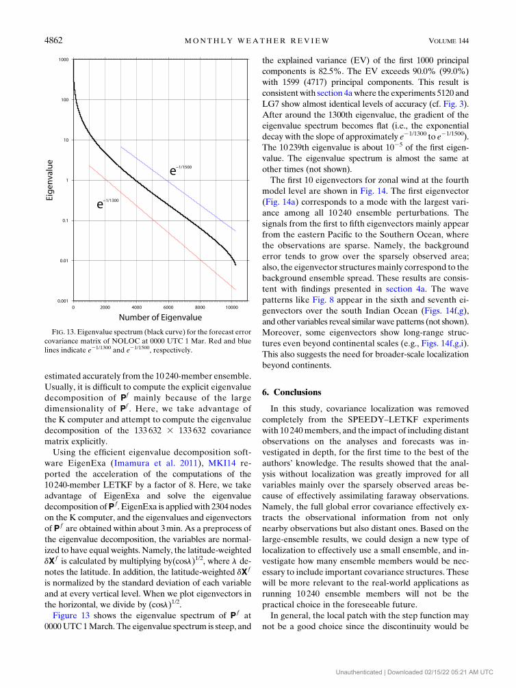
Figure 13 shows the eigenvalue spectrum of P f at

0000UTC1March. The eigenvalue spectrum is steep, and

the explained variance (EV) of the first 1000 principal

components is 82.5%. The EV exceeds 90.0% (99.0%)

with 1599 (4717) principal components. This result is

consistentwith section 4awhere the experiments 5120 and

LG7 show almost identical levels of accuracy (cf. Fig. 3).

After around the 1300th eigenvalue, the gradient of the

eigenvalue spectrum becomes flat (i.e., the exponential

decay with the slope of approximately e21/1300 to e21/1500).

The 10239th eigenvalue is about 1025 of the first eigen-

value. The eigenvalue spectrum is almost the same at

other times (not shown).

The first 10 eigenvectors for zonal wind at the fourth

model level are shown in Fig. 14. The first eigenvector

(Fig. 14a) corresponds to a mode with the largest vari-

ance among all 10 240 ensemble perturbations. The

signals from the first to fifth eigenvectors mainly appear

from the eastern Pacific to the Southern Ocean, where

the observations are sparse. Namely, the background

error tends to grow over the sparsely observed area;

also, the eigenvector structuresmainly correspond to the

background ensemble spread. These results are consis-

tent with findings presented in section 4a. The wave

patterns like Fig. 8 appear in the sixth and seventh ei-

genvectors over the south Indian Ocean (Figs. 14f,g),

and other variables reveal similarwave patterns (not shown).

Moreover, some eigenvectors show long-range struc-

tures even beyond continental scales (e.g., Figs. 14f,g,i).

This also suggests the need for broader-scale localization

beyond continents.

6. Conclusions

In this study, covariance localization was removed

completely from the SPEEDY–LETKF experiments

with 10 240members, and the impact of including distant

observations on the analyses and forecasts was in-

vestigated in depth, for the first time to the best of the

authors’ knowledge. The results showed that the anal-

ysis without localization was greatly improved for all

variables mainly over the sparsely observed areas be-

cause of effectively assimilating faraway observations.

Namely, the full global error covariance effectively ex-

tracts the observational information from not only

nearby observations but also distant ones. Based on the

large-ensemble results, we could design a new type of

localization to effectively use a small ensemble, and in-

vestigate how many ensemble members would be nec-

essary to include important covariance structures. These

will be more relevant to the real-world applications as

running 10 240 ensemble members will not be the

practical choice in the foreseeable future.

In general, the local patch with the step function may

not be a good choice since the discontinuity would be

FIG. 13. Eigenvalue spectrum (black curve) for the forecast error

covariance matrix of NOLOC at 0000 UTC 1 Mar. Red and blue

lines indicate e21/1300 and e21/1500, respectively.

4862 MONTHLY WEATHER REV IEW VOLUME 144

Unauthenticated | Downloaded 02/15/22 05:21 AM UTC

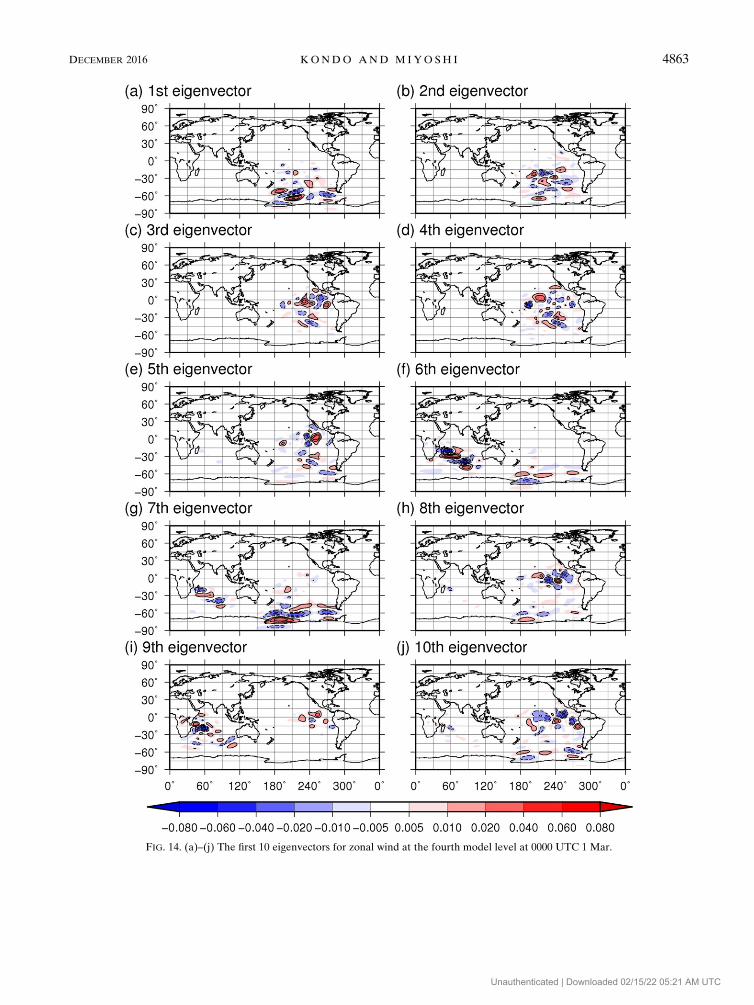
FIG. 14. (a)–(j) The first 10 eigenvectors for zonal wind at the fourth model level at 0000 UTC 1 Mar.

DECEMBER 2016 KONDO AND M IYO SH I 4863

Unauthenticated | Downloaded 02/15/22 05:21 AM UTC

problematic. Oczkowski et al. (2005), Kuhl et al. (2007),

and Satterfield and Szunyogh (2010, 2011) discussed the

ensemble E dimension using the ensemble size up to

about 150. This study is somewhat different from pre-

vious examples because of the orders of magnitude

larger ensemble size, which allowed us to apply the

larger-scale local patches and Gaussian function locali-

zation without severe problems.

The ensemble size of 10 240 is very close to 10 816, the

number of observations, so that the ensemble nearly

spans the observation space. This is not usually the case

in the real atmosphere, where the number of observa-

tions is much larger than 105. It is an open question if no

localization is a better choice when the ensemble can

span only a fraction of the observation space. This

should be investigated in future research efforts.

This study focused on the impact of localization and

different ensemble sizes. Recently, using a hybrid

covariance matrix between climatological component

and ensemble-based flow-dependent component

became a viable choice in the operational systems

(Hamill and Snyder 2000; Wang et al. 2013; Kleist and

Ide 2015; Clayton et al. 2013). It would be an in-

teresting future issue to investigate the effects of in-

cluding climatological components to represent the

large scale covariance structure, compared with the

flow-dependent covariance structure estimated with

the large ensemble.

The experiments in this study were implemented un-

der the perfect model scenario and were only simula-

tions, not representing the real atmosphere. Also, the

SPEEDY model is an intermediate AGCM with simpli-

fied physics and resolves only up to 30 horizontal wave-

numbers with seven vertical levels. Higher-resolution

models represent finer-scale structures, and the eigen-

value spectrum should be less steep. Hence, the rank of

the background error covariance matrix would be larger,

and a larger ensemble size would be necessary. Yet,

Miyoshi et al. (2015) reported that their 10 240-member

LETKF experiments for the real atmosphere also

showed long-range error correlations with real-world

observations using the state-of-the-art NICAM at

112-km resolution with 40 vertical levels. An important

next step would be to investigate if including distant

observations helps improve the real-world NWP.

Acknowledgments. The EigenExa software (http://

www.aics.riken.jp/labs/lpnctrt/EigenExa_e.html) plays an

essential role in solving the eigenvalues for 10240 310240 dense real symmetric matrices and is kindly pro-

vided by T. Imamura of Large-Scale Parallel Numerical

Computing Technology Research Team, RIKEN AICS.

The SPEEDY–LETKF code is publicly available online

(http://code.google.com/p/miyoshi/). We are grateful to

the members of the Data Assimilation Research Team,

RIKEN AICS, for fruitful discussions. Results were, in

part, obtained by using the K computer at the RIKEN

AICS through Proposals ra000015 and hp150019. This

study was partly supported by CREST, JST, and JSPS

KAKENHI Grant JP16K17806.

REFERENCES

Bishop, C. H., B. J. Etherton, and S. J. Majumdar, 2001: Adaptive

sampling with the ensemble transform Kalman filter. Part I:

Theoretical aspects. Mon. Wea. Rev., 129, 420–436, doi:10.1175/

1520-0493(2001)129,0420:ASWTET.2.0.CO;2.

——, C. A. Reynolds, andM. K. Tippett, 2003: Optimization of the

fixed global observing network in a simple model. J. Atmos.

Sci., 60, 1471–1489, doi:10.1175/1520-0469(2003)060,1471:

OOTFGO.2.0.CO;2.

Clayton, A.M., A. C. Lorenc, andD.M. Barker, 2013: Operational

implementation of a hybrid ensemble/4D-Var global data as-

similation system at the Met Office. Quart. J. Roy. Meteor.

Soc., 139, 1445–1461, doi:10.1002/qj.2054.

Evensen, G., 1994: Sequential data assimilation with a nonlinear

quasi-geostrophic model using Monte Carlo methods to

forecast error statistics. J. Geophys. Res., 99, 10 143–10 162,

doi:10.1029/94JC00572.

Flowerdew, J., 2015: Towards a theory of optimal localisation.

Tellus, 67A, 25257, doi:10.3402/tellusa.v67.25257.

Gaspari, G., and S. E. Cohn, 1999: Construction of correlation

functions in two and three dimensions. Quart. J. Roy. Meteor.

Soc., 125, 723–757, doi:10.1002/qj.49712555417.

Greybush, S. J., E. Kalnay, T.Miyoshi, K. Ide, and B. R.Hunt, 2011:

Balance and ensemble Kalman filter localization techniques.

Mon. Wea. Rev., 139, 511–522, doi:10.1175/2010MWR3328.1.

Hamill, T. M., and C. Snyder, 2000: A hybrid ensemble Kalman

filter–3D variational analysis scheme. Mon. Wea. Rev.,

128, 2905–2919, doi:10.1175/1520-0493(2000)128,2905:

AHEKFV.2.0.CO;2.

——, J. S. Whitakaer, and C. Snyder, 2001: Distance-dependent

filtering of background error covariance estimates in an en-

semble Kalman filter. Mon. Wea. Rev., 129, 2776–2790,

doi:10.1175/1520-0493(2001)129,2776:DDFOBE.2.0.CO;2.

Houtekamer, P. L., and H. L. Mitchell, 1998: Data assimila-

tion using an ensemble Kalman filter technique. Mon. Wea.

Rev., 126, 796–811, doi:10.1175/1520-0493(1998)126,0796:

DAUAEK.2.0.CO;2.

Hunt, B. R., E. J. Kostelich, and I. Syzunogh, 2007: Efficient data

assimilation for spatiotemporal chaos: A local ensemble

transformKalman filter. Physica D, 230, 112–126, doi:10.1016/

j.physd.2006.11.008.

Imamura, T., S. Yamada, and M. Machida, 2011: Development of a

high performance eigensolver on the peta-scale next-generation

supercomputer system. Prog. Nucl. Sci. Technol., 2, 643–650,

doi:10.15669/pnst.2.643.

Kalman, R. E., 1960: A new approach to linear filtering and pre-

dicted problems. J. Basic Eng., 82, 35–45, doi:10.1115/

1.3662552.

Kang, J.-S., E. Kalnay, T. Miyoshi, J. Liu, and I. Fung, 2012: Esti-

mation of surface carbon fluxes with an advanced data as-

similation methodology. J. Geophys. Res., 117, D24101,

doi:10.1029/2012JD018259.

4864 MONTHLY WEATHER REV IEW VOLUME 144

Unauthenticated | Downloaded 02/15/22 05:21 AM UTC

Kleist, D. T., and K. Ide, 2015: An OSSE-based evaluation of hy-

brid variational–ensemble data assimilation for the NCEP

GFS. Part I: System description and 3D-hybrid results. Mon.

Wea. Rev., 143, 433–451, doi:10.1175/MWR-D-13-00351.1.

Kondo, K., and H. L. Tanaka, 2009: Applying the local ensemble

transform Kalman filter to the Nonhydrostatic Icosahedral

AtmosphericModel (NICAM).SOLA, 5, 121–124, doi:10.2151/

sola.2009-031.

——, T. Miyoshi, and H. L. Tanaka, 2013: Parameter sensitivities

of the dual-localization approach in the local ensemble

transform Kalman filter. SOLA, 9, 174–178, doi:10.2151/

sola.2013-039.

Kuhl, D., and Coauthors, 2007: Assessing predictability with a

local ensemble Kalman filter. J. Atmos. Sci., 64, 1116–1140,

doi:10.1175/JAS3885.1.

Kunii, M., 2014: Mesoscale data assimilation for a local severe

rainfall event with the NHM-LETKF system. Wea. Fore-

casting, 29, 1093–1105, doi:10.1175/WAF-D-13-00032.1.

Ménétrier, B., T. Montmerle, Y. Michel, and L. Berre, 2015a:

Linear filtering of sample covariances for ensemble-based

data assimilation. Part I: Optimality criteria and application to

variance filtering and covariance localization.Mon.Wea. Rev.,

143, 1622–1643, doi:10.1175/MWR-D-14-00157.1.

——, ——, ——, and ——, 2015b: Linear filtering of sample co-

variances for ensemble-based data assimilation. Part II: Ap-

plication to a convective-scale NWP model. Mon. Wea. Rev.,

143, 1644–1664, doi:10.1175/MWR-D-14-00156.1.

Miyoshi, T., 2005: Ensemble Kalman filter experiments with a

primitive-equation global model. Ph.D. thesis, University of

Maryland, College Park, 226 pp. [Available online at http://

drum.lib.umd.edu/handle/1903/3046.]

——, 2011: TheGaussian approach to adaptive covariance inflation

and its implementation with the local ensemble transform

Kalman filter. Mon. Wea. Rev., 139, 1519–1535, doi:10.1175/2010MWR3570.1.

——, and S. Yamane, 2007: Local ensemble transform Kalman

filtering with an AGCM at a T159/L48 resolution. Mon. Wea.

Rev., 135, 3841–3861, doi:10.1175/2007MWR1873.1.

——, and M. Kunii, 2012: The local ensemble transform Kalman

filter with the Weather Research and Forecasting Model:

Experiments with real observations. Pure Appl. Geophys.,

169, 321–333, doi:10.1007/s00024-011-0373-4.

——, and K. Kondo, 2013: A multi-scale localization approach to

an ensemble Kalman filter. SOLA, 9, 170–173, doi:10.2151/

sola.2013-038.

——, S. Yoshiaki, and T. Kadowaki, 2010: Ensemble Kalman filter

and 4D-Var intercomparison with the Japanese operational

global analysis and prediction system. Mon. Wea. Rev., 138,

2846–2866, doi:10.1175/2010MWR3209.1.

——, K. Kondo, and T. Imamura, 2014: 10240-member ensemble

Kalman filtering with an intermediate AGCM.Geophys. Res.

Lett., 41, 5264–5271, doi:10.1002/2014GL060863.

——, ——, and K. Terasaki, 2015: Numerical weather prediction

with big ensemble data assimilation. Computer, 48, 15–21,

doi:10.1109/MC.2015.332.

Molteni, F., 2003: Atmospheric simulations using a GCM with

simplified physical parametrizations. I: Model climatology and

variability in multi-decadal experiments. Climate Dyn., 20,

175–191, doi:10.1007/s00382-002-0268-2.

Oczkowski, M., I. Szunyogh, and D. J. Patil, 2005: Mechanisms for

the development of locally low dimensional atmospheric dy-

namics. J. Atmos. Sci., 62, 1135–1156, doi:10.1175/JAS3403.1.

Ott, E., and Coauthors, 2004: A local ensemble Kalman filter for

atmospheric data assimilation.Tellus, 56A, 415–428, doi:10.1111/

j.1600-0870.2004.00076.x.

Perianez, A., H. Reich, and R. Potthast, 2014: Optimal localization

for ensemble Kalman filter systems. J. Meteor. Soc. Japan, 92,585–597, doi:10.2151/jmsj.2014-605.

Rainwater, S., and B. Hunt, 2013: Mixed-resolution ensemble data

assimilation. Mon. Wea. Rev., 141, 3007–3021, doi:10.1175/

MWR-D-12-00234.1.

Satoh,M., T.Matsuno, H. Tomita, H.Miura, T. Nasuno, and S. Iga,

2008: Nonhydrostatic Icosahedral Atmospheric Model

(NICAM) for global cloud resolving simulations. J. Comput.

Phys., 227, 3486–3514, doi:10.1016/j.jcp.2007.02.006.——, and Coauthors, 2014: The Non-hydrostatic Icosahedral At-

mospheric Model: Description and development. Prog. Earth

Planet. Sci., 1, 18, doi:10.1186/s40645-014-0018-1.Satterfield, E. A., and I. Szunyogh, 2010: Predictability of the

performance of an ensemble forecast system: Predictability of

the space of uncertainties. Mon. Wea. Rev., 138, 962–981,

doi:10.1175/2009MWR3049.1.

——, and ——, 2011: Assessing the performance of an ensemble

forecast system in predicting the magnitude and the spectrum

of analysis and forecast uncertainties. Mon. Wea. Rev., 139,

1207–1223, doi:10.1175/2010MWR3439.1.

Terasaki, K., M. Sawada, and T. Miyoshi, 2015: Local ensemble

transform Kalman filter experiments with the Nonhydrostatic

Icosahedral Atmospheric Model NICAM. SOLA, 11, 23–26,doi:10.2151/sola.2015-006.

Wang, X., D. Parrish, D. Kleist, and J. Whitaker, 2013: GSI

3DVar-based ensemble–variational hybrid data assimila-

tion for NCEP global forecast system: Single-resolution ex-

periments. Mon. Wea. Rev., 141, 4098–4117, doi:10.1175/

MWR-D-12-00141.1.

Yussouf, N., andD. J. Stensrud, 2010: Impact of phased-array radar

observations over a short assimilation period: Observing sys-

tem simulation experiments using an ensemble Kalman filter.

Mon. Wea. Rev., 138, 517–538, doi:10.1175/2009MWR2925.1.

Zhang, F., Y. Weng, J. A. Sippel, Z. Meng, and C. H. Bishop, 2009:

Cloud-resolving hurricane initialization and prediction through

assimilation of Doppler radar observations with an ensemble

Kalman filter. Mon. Wea. Rev., 137, 2105–2125, doi:10.1175/

2009MWR2645.1.

DECEMBER 2016 KONDO AND M IYO SH I 4865

Unauthenticated | Downloaded 02/15/22 05:21 AM UTC