Maximum likelihood estimation of covariance parameters … · Maximum likelihood estimation of covariance ... variables estimated ... Maximum likelihood estimation of covariance parameters

Maximum likelihood estimation of covariance parameters for

Bayesian atmospheric trace gas surface flux inversions

Anna M. Michalak,1,2 Adam Hirsch,3,4 Lori Bruhwiler,3 Kevin R. Gurney,5

Wouter Peters,3,4 and Pieter P. Tans3

Received 15 March 2005; revised 26 July 2005; accepted 31 August 2005; published 23 December 2005.

[1] This paper introduces a Maximum Likelihood (ML) approach for estimating thestatistical parameters required for the covariance matrices used in the solution of Bayesianinverse problems aimed at estimating surface fluxes of atmospheric trace gases. Themethod offers an objective methodology for populating the covariance matrices requiredin Bayesian inversions, thereby resulting in better estimates of the uncertainty associatedwith derived fluxes and minimizing the risk of inversions being biased by unrealisticcovariance parameters. In addition, a method is presented for estimating the uncertaintyassociated with these covariance parameters. The ML method is demonstrated using atypical inversion setup with 22 flux regions and 75 observation stations from the NationalOceanic and Atmospheric Administration-Climate Monitoring and DiagnosticsLaboratory (NOAA-CMDL) Cooperative Air Sampling Network with available monthlyaveraged carbon dioxide data. Flux regions and observation locations are binnedaccording to various characteristics, and the variances of the model-data mismatch and ofthe errors associated with the a priori flux distribution are estimated from the availabledata.

Citation: Michalak, A. M., A. Hirsch, L. Bruhwiler, K. R. Gurney, W. Peters, and P. P. Tans (2005), Maximum likelihood estimation

of covariance parameters for Bayesian atmospheric trace gas surface flux inversions, J. Geophys. Res., 110, D24107,

doi:10.1029/2005JD005970.

1. Introduction

[2] The use of inverse modeling methods as tools forestimating fluxes of atmospheric trace gases has becomeincreasingly common as the need to constrain theirglobal and regional budgets has been recognized[Intergovernmental Panel on Climate Change (IPCC),2001; Committee on the Science of Climate Change,Division on Earth and Life Studies, National ResearchCouncil, 2001; Wofsy and Harriss, 2002]. Inverse methodsattempt to deconvolute the effects of atmospheric transportand recover source fluxes (typically surface fluxes) based onatmospheric measurements. Information about regions thatare not being directly sampled can potentially be inferredfrom downwind atmospheric measurements. Inversemodeling methods have been used to estimate regionalcontributions to global budgets of trace gases such as

CFCs, CH4, and CO2, and a review of recent applications ispresented by Enting [2002, chap. 14–17].[3] A vast majority of recent inverse modeling studies

have relied on a classical Bayesian approach, where thesolution to the inverse problem is defined as the set of fluxvalues that represent an optimal balance between tworequirements. The first criterion is that the optimized, or aposteriori, fluxes should be as close as possible to the first-guess (a priori) fluxes. The second is that the measurementvalues that would result from the inversion-derived(a posteriori) fluxes should agree as closely as possiblewith the actual measured concentrations. For the case wherethe advection scheme is linear, this solution corresponds tothe minimum of a cost function Ls defined as:

Ls ¼1

2z�Hsð ÞTR�1 z�Hsð Þ þ 1

2s� sp� �T

Q�1 s� sp� �

; ð1Þ

where z is an n � 1 vector of observations, H is an n � mJacobian matrix representing the sensitivity of the observa-tions z to the function s (i.e., Hi,j = @zi/@sj), s is an m � 1vector of the discretized unknown surface flux distribution,R is the n � n model-data mismatch covariance, sp is them � 1 prior estimate of the flux distribution s, Q is thecovariance of the errors associated with the prior estimatesp, and the superscript T denotes the matrix transposeoperation. A solution in the form of a superposition of allstatistical distributions involved can be computed, fromwhich a posteriori means and covariances can be derived

JOURNAL OF GEOPHYSICAL RESEARCH, VOL. 110, D24107, doi:10.1029/2005JD005970, 2005

1Department of Civil and Environmental Engineering, University ofMichigan, Ann Arbor, Michigan, USA.

2Also at Department of Atmospheric, Oceanic and Space Sciences,University of Michigan, Ann Arbor, Michigan, USA.

3Climate Monitoring and Diagnostics Laboratory, NOAA, Boulder,Colorado, USA.

4Also at Cooperative Institute for Research in Environmental Sciences,University of Colorado, Boulder, Colorado, USA.

5Department of Atmospheric Science, Colorado State University, FortCollins, Colorado, USA.

Copyright 2005 by the American Geophysical Union.0148-0227/05/2005JD005970

D24107 1 of 16

[e.g., Enting et al., 1995]. The solution is [Tarantola,1987; Enting, 2002],

s ¼ sp þQHT HQHT þ R� ��1

z�Hsp� �

ð2Þ

Vs ¼ Q�QHT HQHT þ R� ��1

HQ; ð3Þ

where s is the posterior best estimate of s, and Vs is itsposterior covariance.[4] In most Bayesian studies, both R and Q have been

modeled as diagonal matrices. In this case, the diagonalelements of R represent the model-data mismatch varianceof each observation, which is the sum of the variancesassociated with all error components such as, for instance,the observation error, the transport modeling error, and therepresentation error. The diagonal elements of Q, on theother hand, represent the error variance of the prior fluxestimates and specify the extent to which the real fluxes areexpected to deviate from prior flux estimates. It is importantto note that although the vast majority of Bayesian inversionstudies have used diagonal covariance matrices, some errorsare known to be both temporally and spatially correlated.[5] One of the challenges of the Bayesian approach is the

need to estimate the parameters defining the model-datamismatch covariance matrix R and the prior error covari-ance matrix Q. These covariances determine the relativeweight of prior information versus available data in esti-mating individual fluxes, and are therefore key componentsin estimating the posterior covariance (and thereby theuncertainty) of these fluxes. As a result, identifying appro-priate covariance parameters is essential to accurate fluxestimation. The importance and challenge of accuratelyestimating these parameters [Kaminski et al., 1999; Rayneret al., 1999; Law et al., 2002; Peylin et al., 2002; Engelen etal., 2002] and the lack of objective methods for doing so[Rayner et al., 1999] have been increasingly recognized inthe literature.[6] Past inversion studies have relied on a variety of

methods for estimating these parameters. In the originalsynthesis inversion work of Enting et al. [1995], the datauncertainty was based on a statistical characteristics of theNOAA flask sampling procedures [Tans et al., 1990], butthe uncertainty associated with errors in the atmospherictransport model could not be quantified. Many more recentstudies have derived model-data mismatch from the residualstandard deviation of flask samples around a smooth curvefit [e.g., Hein et al., 1997; Bousquet et al., 1999; Gurney etal., 2002; Peylin et al., 2002]. Others have relied on valuesindependently obtained from the literature [e.g., Kandlikar,1997]. The a priori flux errors have been even more difficultto quantify [Kaminski et al., 1999], and the choice of priorerrors has even been described as ‘‘mostly arbitrary’’ insome studies [Bousquet et al., 1999], even though it isrecognized that these parameters are crucial to the inversion.Often, researchers have applied what are considered to be‘‘loose’’ priors [e.g., Peylin et al., 2002; Law et al., 2002] inorder to yield conservative estimates of the flux uncertain-ties. On the basis of assessments of available data, oceanicfluxes have usually been considered more certain thanterrestrial fluxes [e.g., Kaminski et al., 1999]. Althoughconsiderable effort has been put into estimating covarianceparameters, the specification of the prior uncertainties has

been described as the ‘‘greatest single weakness’’ in somestudies [Rayner et al., 1999].[7] Recently, several researchers have scaled the model-

data mismatch and/or prior error covariance parameters toobtain a data misfit function that follows a c2 distributionwith a given number of degrees of freedom [e.g., Rayneret al., 1999; Gurney et al., 2002; Peylin et al., 2002;Rodenbeck et al., 2003]. The correct number of degreesof freedom to be used in such an analysis is equal to thetotal number of independent pieces of information intro-duced into the system (equal to the number of observa-tional data plus the number of prior flux estimates in thecase of diagonal Q and R matrices), minus the number ofvariables estimated in the inversion (typically equal to thenumber of estimated fluxes). If the covariance parametersare reasonable, the sum of the squared residuals, scaledby their uncertainties and normalized by the number ofdegrees of freedom, should be close to 1 (reduced chi-squared cr

2 = 1). Some researchers have applied this testto the residuals between the available observations andthose that would result from the a posteriori fluxesobtained from the inversion, while others have applied it bothto these observation residuals and to residuals of the aposteriori fluxes from their prior estimates. Such tuning,however, does not yield a unique solution because more thanone combination of covariance parameters can lead to theresiduals having an acceptable cr

2. In addition, looking at thecr2 cannot guide the relative allocation of error between

the model-data mismatch and prior flux estimates [Rayneret al., 1999]. Therefore examining the variance of theresiduals is a necessary, but not a sufficient, condition forevaluating the appropriateness of covariance parameters.[8] A few recent studies have attempted to systematically

quantify one or more components of the model-data mis-match. Engelen et al. [2002] divided the model-data mis-match covariance into four additive covariances (whichwere modeled as diagonal matrices) representing: (1) theobservation error, (2) the error in mapping concentrations ata specific location into the measured quantity, (3) the modeltransport error, and (4) the representation error describingthe effects of model resolution. Each of these error sourceswas then quantified based either on available additionalinformation (e.g., known precision of analytical methods) ornumerical experiments (e.g., comparing inversion resultsobtained using various transport models in order to estimatetransport error). Kaminski et al. [2001] focused on the errorsintroduced as a result of imposing potentially erroneousfixed flux patterns within regions, and estimated the addi-tional variance that should be added to the model-datamismatch covariance to account for this effect. Krakaueret al. [2004] estimated single scaling factors for both themodel-data mismatch and prior error covariances using ageneralized cross-validation approach, to show that theTranscom inversion results for the global land/ocean parti-tioning, particularly in the Southern Hemisphere and trop-ical regions, were influenced strongly by the Transcomchoice of parameters. The fluxes resulting from this analysisand their associated residuals were not analyzed to deter-mine whether these parameters result in fluxes that areconsistent with the underlying statistical assumptions, andthe uncertainty associated with the estimated covarianceparameters was not quantified.

D24107 MICHALAK ET AL.: COVARIANCE PARAMETERS FOR FLUX INVERSION

2 of 16

D24107

[9] The method that will be developed in this paperallows the available data to shed light on the covarianceparameters to be used in the inversion, both in defining themodel-data mismatch and the error associated with the priorflux distribution. This can be done in a consistent manner byidentifying the Maximum Likelihood (ML) estimates ofthese parameters, given the prior flux estimates sp, theavailable measurements z, and the sensitivity H of thesemeasurements to the fluxes to be estimated. The method isapplicable whenever estimates of the covariance parametersare to be obtained from the atmospheric data themselves. AML approach has previously been used in estimating spatialdrift and covariance parameters of hydrologic variables,based on limitedmeasurements of these parameters [Kitanidisand Lane, 1985]. Also, a related restricted maximum likeli-hood (RML) approach has been used for estimating covari-ance parameters in geostatistical inverse modeling [e.g.,Kitanidis, 1995; Michalak and Kitanidis, 2004]. Recently,this technique was applied to the estimation of covarianceparameters in a geostatistical implementation of the atmo-spheric trace-gas inversion problem [Michalak et al., 2004].In this paper, we develop and demonstrate a maximumlikelihood methodology for estimating the model-data mis-match and prior-error covariancematrix parameters needed inthe application of the classical Bayesian inverse modelingapproach. This method can be directly applied to all studieswhere the objective function is of the form presented inequation (1), which is themost common setup currently beingused in atmospheric inversion studies. This method allows,for the first time, for an objective and data-driven estimationof both the model-data mismatch and prior error covarianceparameters required for the solution of the flux estimationinverse problem. Several covariance parameters can be esti-mated simultaneously, the resulting fluxes yield residuals thatfollow the assumed distribution (e.g., cr

2 = 1), and theuncertainty associated with the covariance parameters canalso be estimated. In the sample application presented in thiswork, bothR andQ are modeled as diagonal matrices, but themethod is directly applicable to cases where these matricesinclude spatial and temporal correlation (i.e., off-diagonalterms). In such cases, parameters such as the correlationlength of flux deviations from their prior estimates can alsobe estimated.

2. Maximum Likelihood Estimation

[10] We are interested in finding the maximum likelihoodestimate of the model-data mismatch and prior error covari-ance parameters in Bayesian inverse modeling. Note thatthroughout this discussion, the term prior errors refers to theerrors between the actual fluxes and the prior flux estimates. Inthe case where both the model-data mismatch matrix and theprior error covariance matrix are diagonal matrices of varian-ces, this can be thought of as optimizing the variances in

R ¼

s2R;1 0 � � � 0

0 s2R;2...

..

. . ..

0

0 � � � 0 s2R;n

2666664

3777775;Q ¼

s2Q;1 0 � � � 0

0 s2Q;2...

..

. . ..

0

0 � � � 0 s2Q;m

2666664

3777775;

ð4Þ

where sR,i2 are the model-data mismatch variances of

individual observations and sQ,i2 are the prior-error variances

of individual prior flux estimates. In the simplest case, wecould assume that a single variance describes the model-data mismatch at all sites, and another variance describesthe prior error for all source regions, yielding a total of twoparameters to be estimated. On the other end of thespectrum, a different model-data mismatch could beestimated for each measurement location and each sourceregion. Other options would be to populate the covariancematrices with scaling factors that we believe to berepresentative of the relative errors of certain measurementsor priors and solve for overall proportionality constants thatwould adjust the magnitude of these variances, or toestimate the covariance (in space and/or in time) of theerrors. Various options will be demonstrated in section 3 ofthis paper. It is important to note that one would not go asfar as estimating a different variance for each individualflask measurement, because one cannot estimate a varianceusing a single measurement.

2.1. Probability Density Function

[11] We are interested in the probability density functionof the covariance parameters of R and Q, which we willjointly call Q, given the available observations z, the priorestimates sp, and the transport matrix H. In the examplegiven in equation (4) Q = {sR,1

2 ,. . ., sR,n2 , sQ,1

2 ,. . ., sQ,m2 },

which would be binned into subgroups based on fluxregions and measurement stations, and potentially furthergrouped by regions or stations that are expected to havesimilar properties (e.g., marine boundary layer stations).According to Bayes’ rule, the pdf of the parameters Q can bedefined as

p00 QjH; sp; z� �

¼p zjH; sp; Q� �

p0 QjH; sp� �

Rp zjH; sp; Q� �

p0 QjH; sp� �

dQ; ð5Þ

where the denominator is simply a normalizing constantequal to the probability of the data p(zjH, sp), and where aprime denotes a prior distribution while a double primedenotes a posterior distribution. We assume that, a priori,the probability of the parameters Q is uniform over allvalues, p0(QjH,sp) / 1, which corresponds to the assumptionthat we do not have any prior knowledge about theseparameters. Then


/ p zjH; sp; Q� �

; ð6Þ

yielding the likelihood function of Q. In other words, if weassume that we have no prior information on Q, its pdf isdefined by the likelihood of the observations, and the bestestimate corresponds to the set of values that maximize thislikelihood.[12] The observations z are modeled as

z ¼ Hsþ Ez; ð7Þ

where Ez is a vector representing the model-data mismatch,typically modeled as a vector of n � 1 normally distributed


3 of 16

D24107

random numbers with variance(s) defined by the matrix R.A priori, the expected value of z is

E z½ � ¼ E Hsþ EEz½ �¼ Hsp: ð8Þ

The covariance matrix of z is

E z� E z½ �ð Þ z� E z½ �ð ÞTh i

¼ EhHsþ EEz � E Hsþ EEz½ �ð Þ Hsþ EEz � E Hsþ EEz½ �ð ÞT

i

¼ HQHT þ R: ð9Þ

This expected value and covariance can be used to definethe Gaussian probability density function p(zjH, sp, Q),which, from (6) is proportional to p00(QjH, sp, z):


/ p zjH; sp; Q� �

/ HQHTþ R�� 1=2

� exp� 1

2z�Hsp� �T

HQHT þ R� ��1

z�Hsp� ��

; ð10Þ

where j j denotes a matrix determinant, and Q and R arefunctions of Q. Note that the above equation is normallydistributed with respect to z but not Q. Also, this pdf isindependent of the actual flux distribution s.

2.2. Best Estimate

[13] In order to obtain the maximum likelihood estimateof the covariance parameters, we want to maximizeequation (10) with respect to Q, or alternately, minimizeits negative logarithm,

Lq ¼1

2ln HQHT þ R�� þ 1

2z�Hsp� �T

HQHT þ R� ��1

z�Hsp� �

:

ð11Þ

Note that higher variance values inQ andRwill tend to increasethe value of the first term and decrease the value of the secondterm in this equation. The Q values that minimize this overallobjective function are the ML estimates of these parameters.[14] Conceptually, differences between the available

observations and observations predicted by the prior fluxestimates result from two types of error. First, the model-data mismatch error, parameterized by the covariancematrix R, results from random measurement and transporterrors. Second, the prior error that is parameterized by thecovariance matrix Q accounts for more systematic errors inthe predicted observations because, as a result of the mixingthat takes place as gases are transported downwind, error ina single flux region will be sampled at multiple observationlocations. Although these two sources of error cannot beseparated perfectly, the maximum likelihood approachoffers a rigorous method for estimating the contributionsof these two forms of error. Looking at the objectivefunction in equation (11), the model-data mismatch errorin R is included directly in the optimization, whereas theprior error in Q is ‘filtered’ using the transport matrix H.Therefore, the effect of the model-data mismatch isexpected to behave as an independent, identically distributed(i.i.d.) additive error for the case of a diagonalR, whereas the

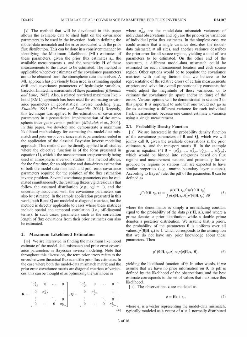
effect of the prior error will have a more systematic effecton a group of observations. The intuitive separationbetween the model-data mismatch and prior error isillustrated in Figure 1.

2.3. Parameter Uncertainty

[15] An estimate of the uncertainty of parameters Q can beobtained from the inverse of the Hessian of equation (11),

Vq ¼ Hij

� ��1; ð12Þ

where the Hessian is defined as

Hij ¼@2Lq

@qi@qjð13Þ

and has dimensions p � p, where p is the total number ofparameters to be estimated. In order to simplify the notation,we define the additional variables,

8 ¼ HQHT þ R ð14Þ

8j ¼ H@Q

@qjHT þ @R

@qjð15Þ

8ij ¼ H@2Q

@qi@qjHT þ @2R

@qi@qj; ð16Þ

which all have dimensions n � n. Also, we will use thefollowing properties [Schweppe, 1973]:

@

@qj8�1 ¼ �8�18j8

�1 ð17Þ

@

@qjln 8j jð Þ ¼ Tr 8�18j

� �; ð18Þ

where Tr is the ‘‘trace’’ operator, which is the sum of thediagonal elements of a matrix. Given these additionalvariables, the Hessian becomes

Hij ¼ � 1

2Tr 8�18i8

�18j

� �þ 1

2Tr 8�18ij

� �þ z�Hsp� �T

8�18i8�18j8

�1 z�Hsp� �

� 1

2z�Hsp� �T

8�18ij8�1 z�Hsp� �

: ð19Þ

Note that in the case where both R and Q are diagonalmatrices of variances, 8ij = [0], and Hij simplifies to

Hij ¼ � 1

2Tr 8�18i8

�18j

� �þ z�Hsp� �T

8�18i8�18j8

�1 z�Hsp� �

: ð20Þ

[16] In some other cases, the second derivative 8ij maybe difficult or expensive to compute, in which case the


4 of 16

D24107

covariance of the parameters can be approximated using theCramer-Rao inequality [Schweppe, 1973] by

Vq � F ij

� ��1; ð21Þ

where F ij is the Fisher information matrix and is theexpected value, with respect to z, of the Hessian Hij:

F ij ¼ E Hij

� �¼ � 1

2Tr 8�18i8

�18j

� �þ 1

2Tr 8�18ij

� �

þ Tr 8�18i8�18j8

�1� �

E z�Hsp� �T

z�Hsp� �h i

� 1

2Tr 8�18ij8

�1� �

E z�Hsp� �T

z�Hsp� �h i

¼ 1

2Tr 8�18i8

�18j

� �: ð22Þ

Figure 1. This figure presents a conceptualization of (a) a prior flux estimate and (b, c, d) three possiblescenarios of how actual observations relate to this prior flux (transported to the time when observationsare made). It illustrates the difference between the effects of model-data mismatch error and prior error.The prior estimate of a flux is depicted in Figure 1a. After a given time, the compound is advected(assuming only advection and no mixing) to a downwind location. On the basis of the prior estimate inFigure 1a, the a priori predicted distribution at the new time is presented as the thick line in Figures 1b,1c, and 1d. The effect of model-data mismatch is expected to be relatively independent for eachobservation and is presented in Figure 1b. The effect of prior error in the magnitude of the flux iscorrelated among several observations and is presented in Figure 1c. Their combined effect is presentedin Figure 1d.


5 of 16

D24107

The diagonal elements of Vq represent the uncertainty of theestimates of the covariance parameters, as defined by theirestimation variance. The uncertainty of the covarianceparameters could be incorporated into the subsequentinversion by drawing an ensemble of samples of thecovariance parameters based on their best estimates anduncertainty, and solving the inversion for each set ofparameters [e.g., Kitanidis, 1986].

2.4. Gauss-Newton Method

[17] In general, an iterative method is needed to find theminimum of equation (11) with respect to the vector ofvalues Q. One efficient option is the Gauss-Newton algo-rithm [e.g., Gill et al., 1986]. Starting from an initialestimate of Q denoted Qk the algorithm proceeds as

Qkþ1 ¼ Qk �F�1k gk ; ð23Þ

where F is the expected value, with respect to z, of theHessian H of the likelihood function, Hij and F ij are asdefined in equations (19) and (22), g is a vector of the firstderivatives of the likelihood function Lq with respect to Q,

gj ¼@Lq@qj

¼ 1

2Tr 8�18j

� �� 1

2z�Hsp� �T

8�18j8�1 z�Hsp� �

ð24Þ

and the subscript k in g and F means that they arecalculated using Qk. The indices take on the values i = 1,. . .,p and j = 1,. . ., p, where p is the total number of parametersQ to be estimated. Note that gk is calculated using the latestestimate Qk. In the special case where both R and Q arelinear in Q, gk is a constant vector.

2.5. Method Validation

[18] In order to demonstrate and validate the proposedmethod, sample applications are presented in the section 3.For each case, once the covariance parameters and theiruncertainties have been estimated, the results are examinedby performing a standard Bayesian inversion (equations (2)and (3)) using the estimated parameters. The residuals fromthese inversions are analyzed to ensure that the method hassuccessfully identified covariance parameters consistentwith the statistical setup of the inversion.[19] As discussed by Tarantola [1987], the squared resid-

uals from the inversions should follow a c2 distribution. Ifboth R and Q are diagonal and the residuals are calculatedusing the posterior best estimate of the flux distribution, thesum of the squared data and flux residuals, normalized bythe variances in R and Q, should follow a c2 distributionwith n degrees of freedom [Tarantola, 1987]. This resultsfrom the fact that the residuals are not independent, andthere are only n degrees of freedom among the n + mresiduals for the case where the R and Q matrices arediagonal. This criterion is applicable to the full set ofresiduals, and cannot be applied directly to only flux orobservation residuals, or to residuals from individual sta-tions or regions. Note that the covariance parameters aretreated as deterministic parameters in the inversion step, andthe number of covariance parameters therefore does notaffect the number of degrees of freedom of the residual c2

distribution.

[20] If, instead of using the best estimates of the fluxes,the residuals from prior fluxes and observations are calcu-lated using conditional realizations of the a posteriori fluxes(see Appendix A), the residuals are expected to follow thestatistical distributions specified in the covariance matricesR and Q. If these matrices are diagonal, this implies that theresiduals from the actual fluxes (and from the conditionalrealizations) are expected to be independent. The conditionalrealizations represent the range of possible flux distributions,given the assumptions and data incorporated into the inver-sion. For the case where residuals are expected to be inde-pendent, the number of degrees of freedom is equal to thenumber of residuals. Therefore the sum of the squaredresiduals from individual conditional realizations, normal-ized by the variances in R and Q, should follow a c2

distribution with n + m degrees of freedom. Moreimportantly, because the residuals should follow thedistributions specified in R and Q, which do not includea cross-covariance between data and flux residuals, ob-servation residuals can be analyzed separately from fluxresiduals to determine whether both the observations andthe prior fluxes are reproduced to the extent assumed bythe parameters in the model-data mismatch and prior errorcovariance matrices. In addition, residuals from individualstations and/or regions can also be analyzed. Whetherresiduals are calculated from the best estimate or condi-tional realizations, the cr

2 statistic (with the appropriatenumber of degrees of freedom) should be equal to 1 inthe case of a sufficiently large number of observations.[21] Once a conditional realization sci has been generated,

the cr2 statistic can be calculated both for the observations

and the prior flux estimates,

c2r;z ¼

1

nz�Hscið ÞTR�1 z�Hscið Þ ð25Þ

c2r;s ¼

1

msci � sp� �T

Q�1 sci � sp� �

; ð26Þ

where cr,z2 is the statistic for the full set of observations used

in the inversion, and cr,s2 is the statistic for the full set of

fluxes estimated in the inversion. As mentioned earlier, acr2 = 1 statistic is not a sufficient condition for identifying

the optimal set of covariance parameters, but it is a necessarycondition. Therefore, although this statistic is not used inestimating the covariance parameters, inversions using theoptimal parameter values should yield residuals with cr

2 = 1.[22] Similarly, a cr

2 statistic can be calculated for indi-vidual stations and/or flux regions. Because we are classi-fying observation locations and flux regions into a smallnumber of groups, we do not expect the cr

2 for individualstations or regions to be exactly equal to one. This isbecause this setup yields a single variance for a subset ofstations/regions, whereas in reality these stations/regionsmay exhibit slightly different error characteristics. Instead,if we have grouped the observation locations and fluxregions in a manner that yields groups with similar charac-teristics, we expect the cr

2 statistic for individual locationsand regions to be distributed around 1. As we allow formore groups (i.e., more estimated covariance parameters)the cr

2 statistic of individual members of these groups willcluster more closely around 1. The cr

2 statistics for individ-


6 of 16

D24107

ual locations (cr,zj2 ) and individual flux regions (cr,sk

2 ) aredefined as

c2r;zj

¼ 1

njzj �Hjsci� �T

R�1j zj �Hjsci� �

ð27Þ

c2r;sk

¼ 1

mk

sci;k � sp;k� �T

Q�1k sci;k � sp;k� �

; ð28Þ

where zj are the observations taken at a given location j, Hj

is the transport matrix relating these observations to allfluxes, Rj is the portion of the model-data mismatchcovariance matrix relating to observations zj, sk are the fluxcomponents for a given region k, sci,k and sp,k are the fluxconditional realization values and the prior flux estimatesfor the same region, and Qk is the portion of the prior errorcovariance matrix relating to fluxes sk.

3. Application to CO2 Data

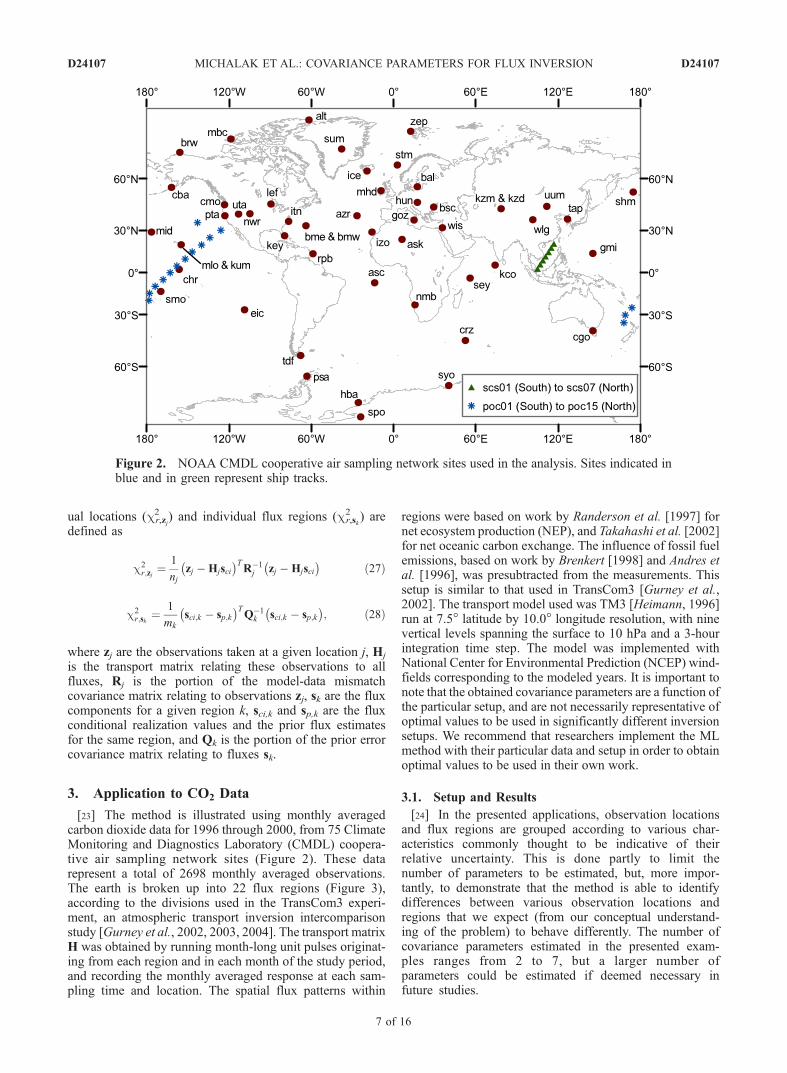
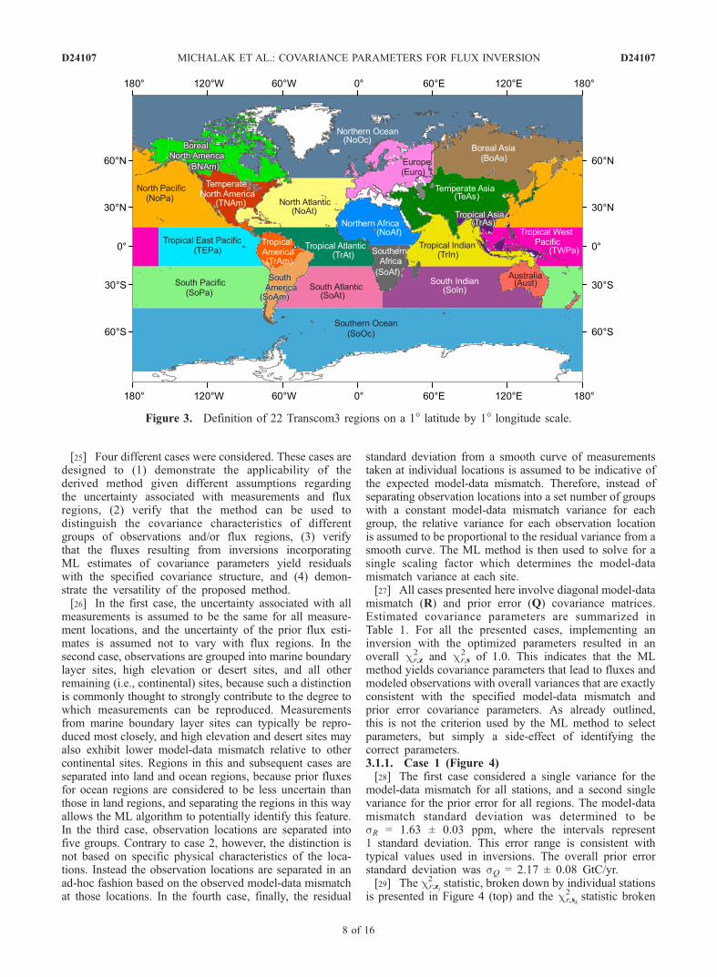
[23] The method is illustrated using monthly averagedcarbon dioxide data for 1996 through 2000, from 75 ClimateMonitoring and Diagnostics Laboratory (CMDL) coopera-tive air sampling network sites (Figure 2). These datarepresent a total of 2698 monthly averaged observations.The earth is broken up into 22 flux regions (Figure 3),according to the divisions used in the TransCom3 experi-ment, an atmospheric transport inversion intercomparisonstudy [Gurney et al., 2002, 2003, 2004]. The transport matrixH was obtained by running month-long unit pulses originat-ing from each region and in each month of the study period,and recording the monthly averaged response at each sam-pling time and location. The spatial flux patterns within

regions were based on work by Randerson et al. [1997] fornet ecosystem production (NEP), and Takahashi et al. [2002]for net oceanic carbon exchange. The influence of fossil fuelemissions, based on work by Brenkert [1998] and Andres etal. [1996], was presubtracted from the measurements. Thissetup is similar to that used in TransCom3 [Gurney et al.,2002]. The transport model used was TM3 [Heimann, 1996]run at 7.5� latitude by 10.0� longitude resolution, with ninevertical levels spanning the surface to 10 hPa and a 3-hourintegration time step. The model was implemented withNational Center for Environmental Prediction (NCEP) wind-fields corresponding to the modeled years. It is important tonote that the obtained covariance parameters are a function ofthe particular setup, and are not necessarily representative ofoptimal values to be used in significantly different inversionsetups. We recommend that researchers implement the MLmethod with their particular data and setup in order to obtainoptimal values to be used in their own work.

3.1. Setup and Results

[24] In the presented applications, observation locationsand flux regions are grouped according to various char-acteristics commonly thought to be indicative of theirrelative uncertainty. This is done partly to limit thenumber of parameters to be estimated, but, more impor-tantly, to demonstrate that the method is able to identifydifferences between various observation locations andregions that we expect (from our conceptual understand-ing of the problem) to behave differently. The number ofcovariance parameters estimated in the presented exam-ples ranges from 2 to 7, but a larger number ofparameters could be estimated if deemed necessary infuture studies.

Figure 2. NOAA CMDL cooperative air sampling network sites used in the analysis. Sites indicated inblue and in green represent ship tracks.


7 of 16

D24107

[25] Four different cases were considered. These cases aredesigned to (1) demonstrate the applicability of thederived method given different assumptions regardingthe uncertainty associated with measurements and fluxregions, (2) verify that the method can be used todistinguish the covariance characteristics of differentgroups of observations and/or flux regions, (3) verifythat the fluxes resulting from inversions incorporatingML estimates of covariance parameters yield residualswith the specified covariance structure, and (4) demon-strate the versatility of the proposed method.[26] In the first case, the uncertainty associated with all

measurements is assumed to be the same for all measure-ment locations, and the uncertainty of the prior flux esti-mates is assumed not to vary with flux regions. In thesecond case, observations are grouped into marine boundarylayer sites, high elevation or desert sites, and all otherremaining (i.e., continental) sites, because such a distinctionis commonly thought to strongly contribute to the degree towhich measurements can be reproduced. Measurementsfrom marine boundary layer sites can typically be repro-duced most closely, and high elevation and desert sites mayalso exhibit lower model-data mismatch relative to othercontinental sites. Regions in this and subsequent cases areseparated into land and ocean regions, because prior fluxesfor ocean regions are considered to be less uncertain thanthose in land regions, and separating the regions in this wayallows the ML algorithm to potentially identify this feature.In the third case, observation locations are separated intofive groups. Contrary to case 2, however, the distinction isnot based on specific physical characteristics of the loca-tions. Instead the observation locations are separated in anad-hoc fashion based on the observed model-data mismatchat those locations. In the fourth case, finally, the residual

standard deviation from a smooth curve of measurementstaken at individual locations is assumed to be indicative ofthe expected model-data mismatch. Therefore, instead ofseparating observation locations into a set number of groupswith a constant model-data mismatch variance for eachgroup, the relative variance for each observation locationis assumed to be proportional to the residual variance from asmooth curve. The ML method is then used to solve for asingle scaling factor which determines the model-datamismatch variance at each site.[27] All cases presented here involve diagonal model-data

mismatch (R) and prior error (Q) covariance matrices.Estimated covariance parameters are summarized inTable 1. For all the presented cases, implementing aninversion with the optimized parameters resulted in anoverall cr,z

2 and cr,s2 of 1.0. This indicates that the ML

method yields covariance parameters that lead to fluxes andmodeled observations with overall variances that are exactlyconsistent with the specified model-data mismatch andprior error covariance parameters. As already outlined,this is not the criterion used by the ML method to selectparameters, but simply a side-effect of identifying thecorrect parameters.3.1.1. Case 1 (Figure 4)[28] The first case considered a single variance for the

model-data mismatch for all stations, and a second singlevariance for the prior error for all regions. The model-datamismatch standard deviation was determined to besR = 1.63 ± 0.03 ppm, where the intervals represent1 standard deviation. This error range is consistent withtypical values used in inversions. The overall prior errorstandard deviation was sQ = 2.17 ± 0.08 GtC/yr.[29] The cr,zj

2 statistic, broken down by individual stationsis presented in Figure 4 (top) and the cr,sk

2 statistic broken

Figure 3. Definition of 22 Transcom3 regions on a 1� latitude by 1� longitude scale.


8 of 16

D24107

down by individual regions is presented in Figure 4 (bot-tom). As can be seen in the figure, the fact that measure-ments taken at some stations cannot be reproduced asprecisely as those from certain other stations cannot becaptured by this simple setup. As a result, a few observationstations, and especially Hungary (HUN), have a large

overall impact on the model-data mismatch variance, be-cause they are much more difficult to reproduce relative toother stations. Also, the Europe flux region deviates from itsprior flux estimate much more strongly than all otherregions. As will be seen in the other cases, however, thiseffect disappears once certain stations such as HUN are

Table 1. Estimated Covariance Parameters for Examined Casesa

Case

Model-Data Mismatch by Station Prior Error by Region

Station Mismatch Region Prior Error

1 all stations sR = 1.63 ± 0.03 ppm All regions sQ = 2.17 ± 0.08 GtC/yr

2 marine boundary layer sR = 0.71 ± 0.02 ppm ocean sQ = 1.07 ± 0.07 GtC/yrhigh elevation and desert sR = 1.49 ± 0.06 ppm land sQ = 2.02 ± 0.12 GtC/yrother sR = 3.16 ± 0.10 ppm

3 subset 1 sR = 0.58 ± 0.01 ppm ocean sQ = 1.21 ± 0.06 GtC/yrsubset 2 sR = 1.04 ± 0.04 ppm land sQ = 1.76 ± 0.10 GtC/yrsubset 3 sR = 1.91 ± 0.07 ppmsubset 4 sR = 4.36 ± 0.23 ppmsubset 5 sR = 7.64 ± 0.72 ppm

4 all stations, weighted sR = 0.11 ± 0.002 ppm ocean sQ = 0.89 ± 0.08 GtC/yrto 5.96 ± 0.13 ppm land sQ = 2.08 ± 0.15 GtC/yr

aIntervals represent 1 standard deviation.

Figure 4. The cr2 statistics calculated from conditional realizations of the a posteriori fluxes resulting

from an inversion with covariance parameters optimized according to case 1. (top) The cr,zj2 for individual

observation stations. (bottom) The cr,sk2 for individual flux regions. The solid lines represent cr

2 = 1.0,which is the mean cr

2 in both panels (across all stations or regions).


9 of 16

D24107

allowed to have higher model-data mismatch variancesrelative to other stations. The covariance parameters esti-mated using this simplest setup still guarantee that, onaverage, measurements and prior flux estimates are repro-duced to the degree prescribed by the covariance parameter.This is evidenced by the fact that, in this and all subsequentcases, implementing an inversion with the optimized param-eters results in an overall cr,z

2 and cr,s2 of 1.0.

3.1.2. Case 2 (Figure 5)[30] The second case broke observation locations into

three groups: Marine boundary layer (MBL) sites, highelevation or desert sites, and other sites. The flux regionswere separated into land regions and ocean regions. There-fore setup 2 required the estimation of a total of fivevariances. The cr,zj

2 and cr,sk

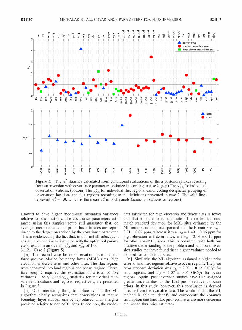
2 statistics for individual mea-surement locations and regions, respectively, are presentedin Figure 5.[31] One interesting thing to notice is that the ML

algorithm clearly recognizes that observations at marineboundary layer stations can be reproduced with a higherprecision relative to non-MBL sites. In addition, the model-

data mismatch for high elevation and desert sites is lowerthan that for other continental sites. The model-data mis-match standard deviation for MBL sites estimated by theML routine and then incorporated into the R matrix is sR =0.71 ± 0.02 ppm, whereas it was sR = 1.49 ± 0.06 ppm forhigh elevation and desert sites, and sR = 3.16 ± 0.10 ppmfor other non-MBL sites. This is consistent with both ourintuitive understanding of the problem and with past inver-sion studies that have found that a higher variance needed tobe used for continental sites.[32] Similarly, the ML algorithm assigned a higher prior

error to land flux regions relative to ocean regions. The priorerror standard deviation was sQ = 2.02 ± 0.12 GtC/yr forland regions, and sQ = 1.07 ± 0.07 GtC/yr for oceanregions. Again, past inversion studies have also assignedgreater uncertainties to the land priors relative to oceanpriors. In this study, however, this conclusion is deriveddirectly from the available data. This confirms that the MLmethod is able to identify and corroborate the commonassumption that land flux prior estimates are more uncertainthat ocean flux prior estimates.



observation stations. (bottom) The cr,sk2 for individual flux regions. Color coding designates grouping of

observation locations and flux regions according to the definitions presented in case 2. The solid linesrepresent cr

2 = 1.0, which is the mean cr2 in both panels (across all stations or regions).


10 of 16

D24107

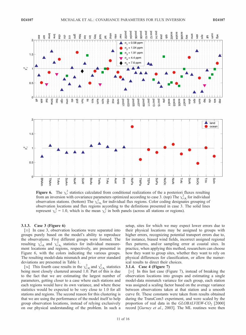
3.1.3. Case 3 (Figure 6)[33] In case 3, observation locations were separated into

groups purely based on the model’s ability to reproducethe observations. Five different groups were formed. Theresulting cr,zj

2 and cr,sk

2 statistics for individual measure-ment locations and regions, respectively, are presented inFigure 6, with the colors indicating the various groups.The resulting model-data mismatch and prior error standarddeviations are presented in Table 1.[34] This fourth case results in the cr,zj

2 and cr,sk

2 statisticsbeing most closely clustered around 1.0. Part of this is dueto the fact that we are estimating the largest number ofparameters, getting closer to a case where each stations andeach regions would have its own variance, and where thesestatistics would be expected to be very close to 1.0 for allstations and regions. The second reason for this clustering isthat we are using the performance of the model itself to helpgroup observation locations, instead of relying exclusivelyon our physical understanding of the problem. In such a

setup, sites for which we may expect lower errors due totheir physical locations may be assigned to groups withhigher errors, recognizing potential transport errors due to,for instance, biased wind fields, incorrect assigned regionalflux patterns, and/or sampling error at coastal sites. Inpractice, when applying this method, researchers can choosehow they want to group sites, whether they want to rely onphysical differences for classification, or allow the numer-ical results to direct their choices.3.1.4. Case 4 (Figure 7)[35] In this last case (Figure 7), instead of breaking the

observation locations into groups and estimating a singlemodel-data mismatch variance for each group, each stationwas assigned a scaling factor based on the average variancebetween observations taken at that station and a smoothcurve fit. These constants were taken from results obtainedduring the TransCom3 experiment, and were scaled by theproportion of real data in the GLOBALVIEW-CO2 [2000]record [Gurney et al., 2003]. The ML routines were then



observation stations. (bottom) The cr,sk2 for individual flux regions. Color coding designates grouping of

observation locations and flux regions according to the definitions presented in case 3. The solid linesrepresent cr

2 = 1.0, which is the mean cr2 in both panels (across all stations or regions).


11 of 16

D24107

used to derive a single proportionality constant that wouldscale these variances to obtain an optimal overall model-data mismatch for each site. The resulting model-datamismatch covariance function was

R ¼

Cs2S;1 0 � � � 0

0 Cs2S;2...

..

. . ..

0

0 � � � 0 Cs2S;n

2666664

3777775; ð29Þ

where sS,i2 are the variances of the deviations of samples

taken at individual sites from a smooth curve fit, and C isthe single multiplicative factor that we will estimate usingthe ML method. The R matrix still has dimensions n � n,where n is the total number of samples considered, but thevalues on the diagonal correspond to the residual variancesobserved at the site where each observation was taken. Theprior error was broken into land and ocean groups, as incases 2 and 3. Note that this final case uses only 41 stations,which are the subset of the examined 75 stations used herewhich were also used in the TransCom3 annual-averageinversion study [Gurney et al., 2003]. This also means thatthere are a total of 41 different variances that populate thematrix in equation (29).

[36] The optimal value of the multiplicative factor wasfound to be 0.80, with a standard deviation of 0.14,indicating that residual standard deviations should be scaledby a factor of

ffiffiffiffiffiffiffiffiffi0:80

p= 0.89 in order to, on average, represent

an appropriate model-data mismatch. The c2r,zj

andcr,sk

2 statistics for individual measurement locations andregions, respectively, are presented in Figure 7. As can beseen from the figure, classification based on the deviationof the observations from a smooth curve is a much betterpredictor of model-data mismatch relative to using aconstant variance for all stations (Figure 4). Better, inthis case refers to the amount of scattering of cr,zj

2 andcr,sk2 around one, because the overall cr,z

2 and cr,s2 are 1.0

for both cases. This last case does not behave as well assubdividing the stations into a moderate number of constant-variance groups (Figure 6), however. For a few stations(HUN, POC13, PSA, SHM in Figure 2) the model-datamismatch appears to be significantly higher relative to thevariance of deviations from a smooth curve as compared toother stations. This is not to say that the variance of thedeviation from a smooth curve could not be used as part ofthe determinant of the relative variance expected at a site,but it does indicate that this criterion may not be effectiveif used as the only guiding principle.[37] Whereas the model-data mismatch standard devia-

tions used in the TransCom3 annual inversion study [Gurney



observation stations. (bottom) The cr,sk2 for individual flux regions. The solid lines represent cr

2 = 1.0,which is the mean cr

2 in both panels (across all stations or regions).


12 of 16

D24107

et al., 2003] ranged from 0.04 ppm (SYO) to 2.23 ppm(ITN), depending on the residual standard deviation ofsamples taken from individual sites from a smooth curvefit, the current analysis suggests that, if all stations areconsidered to have variances proportional to their residualstandard deviations, the model-data mismatch standarddeviations range from 0.11 ppm (SYO) to 5.96 ppm(ITN). The stations with the maximum/minimum model-data mismatch are consistent for these two studies becauseall model-data mismatch standard deviations are determinedby multiplying the residual standard deviations of samplestaken at a given site by a constant factor. Overall, the model-data mismatch variances inferred using the ML method arehigher relative to those used in the TransCom3 annualinversions. This is likely due, at least in part, to the factthat the Transcom study used smoothed Globalview data[GLOBALVIEW-CO2, 2000] in their analysis, whereas thecurrent estimates were obtained using CO2 flask datadirectly. In addition, whereas the Transcom study wasfocusing on annually averaged fluxes, we have insteadestimated monthly fluxes. Additional differences such as theprior flux uncertainties, the selected transport models, andthe subsets of sampling sites used would also contribute tothis difference. Note also that, in the Transcom study, allmodel-data mismatch standard deviations were ultimatelymodified to be at least 0.25 ppm, whereas no suchadjustments were made here.

3.2. Effect on Flux Estimates

[38] The purpose of this work is to present a method forestimating covariance matrix parameters used in Bayesianinversions, and presenting detailed flux estimates for theexamined period falls outside the scope of this work.However, given that each of the sets of covariance param-eters is optimal for its respective setup, it is interesting toexamine the effect of the choice of covariance structure onestimated fluxes.[39] The choice of covariance parameter setup has an

effect on both the flux magnitudes and their estimateduncertainties. The effect on the posterior covariance of thefluxes is relatively straightforward. From equation (3), itis apparent that once a transport model has been selected(thereby fixing H), the covariance matrices fully deter-mine the posterior covariance. What is more difficult toascertain is the effect on the best estimates of the fluxes.

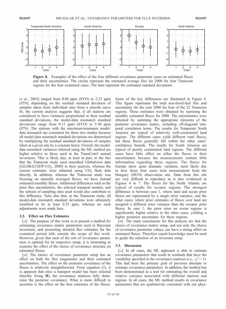
Some of the key differences are illustrated in Figure 8.This figure represents the total non-fossil-fuel flux anduncertainty for the year 2000 for four of the 22 Transcomregions. These estimates were obtained by summing themonthly estimated fluxes for 2000. The uncertainties wereobtained by summing the appropriate elements of theposterior covariance matrix, including off-diagonal tem-poral correlation terms. The results for Temperate NorthAmerica are typical of relatively well-constrained landregions. The different cases yield different total fluxes,but these fluxes generally fall within the other cases’confidence bounds. The results for South America aretypical of poorly constrained land regions. The differentcases have little effect on either the fluxes or theiruncertainties because the measurements contain littleinformation regarding these regions. The fluxes forEurope show quite dramatic variation, most likely dueto how these four cases treat measurement from theHungary (HUN) observation site. Data from this siteare very difficult to reproduce as is also evidenced inFigures 4 to 7. The fluxes for the North Atlantic aretypical of results for oceanic regions. The strongestdifference is between case 1, where land and ocean priorfluxes are represented by a single error variance, and theother cases, where prior estimates of fluxes over land areassigned a different error variance than the oceanic priorfluxes. In case 1, the prior error on ocean regions issignificantly higher relative to the other cases, yielding ahigher posterior uncertainty for these regions.[40] The main conclusions for this analysis are that the

choice of covariance matrix setup, and not only the choiceof covariance parameter values, can have a strong effect onestimated fluxes. Therefore expert knowledge must be usedto guide the selection of an inversion setup.

3.3. Discussion

[41] In all cases, the ML approach is able to estimatecovariance parameters that result in residuals that have thevariability specified in the covariance matrices (i.e., cr

2 = 1).This had been the primary goal of previous attempts toestimate covariance parameters. In addition, the method hasbeen demonstrated as a tool for estimating the overall andrelative variance associated with different stations andregions. In all cases, the ML method results in covarianceparameters that are qualitatively consistent with our phys-

Figure 8. Examples of the effect of the four different covariance parameter cases on estimated fluxesand their uncertainties. The circles represent the estimated average flux for 2000 for four Transcomregions for the four examined cases. The bars represent the estimated standard deviations.


13 of 16

D24107

ical understanding of the relative variance of observationsfrom various stations and fluxes from various regions. Themethod goes beyond this qualitative assessment, however,and quantifies the differing uncertainties associated withindividual stations and/or regions. In addition, the methodwas demonstrated as being an effective guiding tool forgrouping observation locations into groups that behavesimilarly. The method can also incorporate additional infor-mation, such as standard deviations of observations fromsmooth curve fits, into the estimation of covariance param-eters. Last, the method provides uncertainty bounds on thecovariance parameters, which could allow for sensitivityruns exploring the effect of covariance parameter uncertaintyon the estimated flux distributions.[42] As expected and as can be seen from Table 1,

increasing the number of possible variance parametersallows for individual groups of stations or regions to havedifferent behavior. When the grouping corresponds to realdifferences in the model-data mismatch, the cr,zj

2 statistics ofindividual stations are clustered more closely around 1.0, ascan be seen then comparing Figures 4 to 7. It appearsespecially important to assign a different variance to stationsthat are particularly difficult to match, such as Hungary(HUN). Otherwise, as can be seen in Figure 4, these fewstations have too great an influence on the overallcovariance parameters, and as a result most stations havecr,zj2 significantly below 1.[43] Case 3 also demonstrated that one does not neces-

sarily need to separate stations based on our conceptualunderstanding of the difference between various sites, butcan in fact let the model guide group selections, and therebyidentify sites that behave similarly, in terms of the degree towhich their observations can be reproduced given theselected inversion setup.[44] Case 4 demonstrated the possibility of using the ML

algorithm to solve for variance proportionality constants,instead of solving for individual group variances. Futurestudies could explore indices based on other physicalattributes, to determine whether they can predict variabilityat given sites, and whether they can do this better relative tobinning sites into fixed-variance groups, as was done incases 1–3.[45] Finally, as would be expected, the larger the

number of covariance parameters that are to be estimated,the higher their uncertainty. This is a direct result of thefact that, as the number of observation location groupsincreases, there are fewer measurements to constrain thecovariance parameters of each individual group. Overall,however, the uncertainty of the covariance parametersappears quite small. It is important to note that this lowuncertainty is only valid if all the assumptions used in theproblem setup are valid. As is currently typical in fluxinversions we have assumed that model-data mismatcherrors are independent, as are the prior flux errors forlarge regions. In addition, we have binned the covarianceparameters into a relatively small number of representa-tive groups. Therefore the uncertainties on the covarianceparameters should be interpreted in the context of thespecific setup used here. If, for example, a differentmodel-data mismatch uncertainty were to be calculatedfor each observation site, we would expect a higheruncertainty on these parameters relative to the uncertainty

on the covariance parameter averaged over several sites,as was done here.

4. Conclusions

[46] The method presented in this paper uses a maximumlikelihood framework with available observations, prior fluxestimates and transport information to optimize the covari-ance parameters needed in the solution of Bayesian inverseproblems used to estimate surface fluxes of atmospherictrace gases. The method can also be applied to estimate theuncertainty in these parameters. The strong influence andcritical importance of these parameters has been discussedin many studies [Kaminski et al., 1999; Rayner et al., 1999;Law et al., 2002; Peylin et al., 2002; Engelen et al., 2002].Up to this point, however, no objective method was avail-able to estimate these parameters from the available dataand guarantee that the resulting flux and observation resid-uals would follow the assumed distribution.[47] In addition to optimizing covariance parameters for a

given inversion setup, the method can also be used toevaluate whether grouping certain measurement stations orflux regions is justified given the available information. Forexample, if stations are grouped according to whether or notthey constitute marine boundary layer sites, and the result-ing model-data mismatch variances are different for the twogroups, this suggests that whether or not a station samplesmarine boundary layer air is a predictor of the precisionwith which the data can be reproduced.[48] The examples presented in this paper were for

diagonal model-data mismatch and prior error covariancematrices. The method can be directly applied, however, tomore complex covariance matrices, where correlationlengths or other parameters must be estimated in additionto variances. Such applications have been demonstratedusing the restricted maximum likelihood approach used ingeostatistical inverse modeling [Michalak et al., 2004].[49] Note that we do not advocate researchers using the

model-data mismatch variances and prior error variancesderived in this work directly, because the optimal valueswill depend not only on the data set used, but also on thetransport model, the defined flux regions, flux patternswithin regions, etc. Instead, we recommend that researchersimplement the maximum likelihood algorithm described inthis work in order to gain insight into covariance parametersthat are appropriate for their specific applications. Theexamples presented in this work simply demonstrate theapplicability of the presented method to typical inversions.[50] Most importantly, in all the presented cases, the ML

method identified the most likely covariance parametervalues, given the selected inversion setup and covariancematrix definitions. These variances are optimized solelyusing the available data, transport information, and priorflux estimates.

Appendix A: Generation of ConditionalRealizations

[51] If the model-data mismatch and prior-flux errorcovariance parameters are selected appropriately, residualscalculated from conditional realizations of the a posteriorifluxes will follow the distributions specified in Q and R.


14 of 16

D24107

The method presented here generates equally likely condi-tional realizations of the function s. The first step is togenerate an unconditional realization sui of the unknownfunction s from the prior covariance Q. Here the subscript uindicates that the realization has not been conditioned on thedata, and the subscript i serves as a counter and a reminderthat there is an infinite number of possible realizations.There are several methods for generating sui, and themethod presented here is based on eigenvalue decomposi-tion. In the general case,

sui ¼ Vl1=2EEs ðA1Þ

where V is an (m � m) matrix containing the eigenvectorsof Q, l1=2 is an (m � m) diagonal matrix with the squareroot of the eigenvalues of Q on the diagonal, and EEs is an(m � 1) vector of normally distributed random numberswith mean zero and variance one. For the case where Q isa diagonal matrix, as is often the case in classical Bayesianinverse modeling, the above equation simplifies to

sui ¼ Q1=2EEs; ðA2Þ

where Q1/2 is a diagonal matrix with the square root of theprior error variances on the diagonal.[52] The conditional realization is then obtained through

sci ¼ sp þ sui þQHT HQHT þ R� ��1

zþ EEEz �Hsui �Hsp� �

¼ sþ sui þQHT HQHT þ R� ��1

EEz �Hsuið Þ; ðA3Þ

where the subscript c refers to the fact that the realizationhas been conditioned on the data z, and EEz is an (n � 1)vector sampled from the model-data mismatch covariancematrix R, using the same method as was described inequation (A1). The validity of this algorithm can easily bedemonstrated numerically by generating a large number ofconditional realizations and verifying that their statistics(e.g., median and 95% confidence intervals) are identical tothose implied by s and Vs.[53] In addition, substituting the definition of s

(equation (2)) and using the definitions

z ¼ Hsþ EEz ðA4Þ

sp ¼ sþ EEs; ðA5Þ

the expected covariance of residuals from conditionalrealizations can be shown to be

covsci � spHsci � z

� � �¼ Q 0

0 R

� �; ðA6Þ

verifying that, given appropriate covariance parameters, weexpect these residuals to be sampled from Q and R.

[54] Acknowledgments. Funding for Anna Michalak was partiallyprovided by a NOAA Climate and Global Change postdoctoral fellowship,a program administered by the University Corporation for AtmosphericResearch (UCAR). The authors would like to thank all of the collaboratorsin the NOAA/CMDL Cooperative Air Sampling Network, John B. Millerof NOAA-CMDL for helpful insights during the preparation of this

manuscript, and Kimberley L. Mueller for help with figure preparation.This paper was also greatly improved as a result of suggestions offered byIan G. Enting, Peter Rayner, and Christian Rodenbeck.

ReferencesAndres, R. J., G. Marland, I. Fung, and E. Matthews (1996), Distribu-tion of carbon dioxide emissions from fossil fuel consumption andcement manufacture, 1950–1990, Global Biogeochem. Cycles, 10(3),419–430.

Bousquet, P., P. Ciais, P. Peylin, M. Ramonet, and P. Monfray (1999),Inverse modeling of annual atmospheric CO2 sources and sinks: 1. Methodand control inversion, J. Geophys. Res., 104(D21), 26,161–26,178.

Brenkert, A. L. (1998), Carbon dioxide emission estimates from fossil-fuel burning, hydraulic cement production, and gas flaring for 1995 ona one degree grid cell basis, http://cdiac.esd.ornl.gov/ndps/ndp058a.html, Carbon Dioxide Inf. Anal. Cent., Oak Ridge Natl.Lab., Oak Ridge, Tenn.

Committee on the Science of Climate Change, Division on Earth and LifeStudies, National Research Council (2001), Climate Change Science: AnAnalysis of Some Key Questions, Natl. Acad. Press, Washington, D. C.

Engelen, R. J., A. S. Denning, and K. R. Gurney (2002), On error estima-tion in atmospheric CO2 inversions, J. Geophys. Res., 107(D22), 4635,doi:10.1029/2002JD002195.

Enting, I. G. (2002), Inverse Problems in Atmospheric Constituent Trans-port, Cambridge Univ. Press, New York.

Enting, I. G., C. M. Trudinger, and R. J. Francey (1995), A synthesisinversion of the concentration and d13C of atmospheric CO2, Tellus,Ser. B, 47, 35–52.

Gill, P. E., W. Murray, and M. H. Wright (1986), Practical Optimization,Elsevier, New York.

GLOBALVIEW-CO2 (2000), Cooperative Atmospheric Data IntegrationProject—Carbon Dioxide [CD-ROM], NOAA Clim. Model. and Diag.Lab., Boulder, Colo.

Gurney, K. R., et al. (2002), Towards robust regional estimates of CO2

sources and sinks using atmospheric transport models, Nature, 415,626–630, doi:10.1038/415626a.

Gurney, K. R., et al. (2003), TransCom 3 CO2 inversion intercomparison: 1.Annual mean control results and sensitivity to transport and prior fluxinformation, Tellus, Ser. B, 55, 555–579.

Gurney, K. R., et al. (2004), Transcom 3 inversion intercomparison:Model mean results for the estimation of seasonal carbon sourcesand sinks, Global Biogeochem. Cycles, 18, GB1010, doi:10.1029/2003GB002111.

Heimann, M. (1996), The Global Atmospheric Tracer Model TM2, Tech.Rep. 10, 52 pp., Dtsch. Klimarechenzent., Hamburg, Germany.

Hein, R., P. J. Crutzen, and M. Heimann (1997), An inverse modelingapproach to investigate the global atmospheric methane cycle, GlobalBiogeochem. Cycles, 11(1), 43–76.

Intergovernmental Panel on Climate Change (2001), Climate Change 2001:The Scientific Basis, Contribution of Working Group I to the Third As-sessment Report of the Intergovernmental Panel on Climate Change,edited by J. T. Houghton et al., Cambridge Univ. Press, New York.

Kaminski, T., M. Heimann, and R. Giering (1999), A coarse grid three-dimensional global inverse model of the atmospheric transport: 1.Adjoint model and Jacobian matrix, J. Geophys. Res., 104(D15),18,535–18,554.

Kaminski, T., P. J. Rayner, M. Heimann, and I. G. Enting (2001), Onaggregation errors in atmospheric transport inversions, J. Geophys.Res., 106(D5), 4703–4716.

Kandlikar, M. (1997), Bayesian inversion for reconciling uncertainties inglobal mass balances, Tellus, Ser. B, 59, 123–135.

Kitanidis, P. K. (1986), Parameter uncertainty in estimation of spatial func-tions: Bayesian analysis, Water Resour. Res., 22(4), 499–507.

Kitanidis, P. K. (1995), Quasi-linear geostatistical theory for inversing,Water Resour. Res., 31(10), 2411–2419.

Kitanidis, P. K., and R. W. Lane (1985), Maximum likelihood parameterestimation of hydrologic spatial processes by the Gauss-Newton method,J. Hydrol., 79, 53–71.

Krakauer, N. Y., T. Schneider, J. T. Randerson, and S. C. Olsen (2004),Using generalized cross-validation to select parameters in inversions forregional carbon fluxes, Geophys. Res. Lett., 31, L19108, doi:10.1029/2004GL020323.

Law, R. M., R. J. Rayner, L. P. Steele, and I. G. Enting (2002), Using hightemporal frequency data for CO2 inversions, Global Biogeochem. Cycles,16(4), 1053, doi:10.1029/2001GB001593.

Michalak, A. M., and P. K. Kitanidis (2004), Estimation of historicalgroundwater contaminant distribution using the adjoint state method ap-plied to geostatistical inverse modeling, Water Resour. Res., 40, W08302,doi:10.1029/2004WR003214.


15 of 16

D24107

Michalak, A. M., L. Bruhwiler, and P. P. Tans (2004), A geostatisticalapproach to surface flux estimation of atmospheric trace gases, J. Geo-phys. Res., 109, D14109, doi:10.1029/2003JD004422.

Peylin, P., D. Baker, J. Sarmiento, P. Ciais, and P. Bousquet (2002), Influ-ence of transport uncertainty on annual mean and seasonal inversions ofatmospheric CO2 data, J. Geophys. Res., 107(D19), 4385, doi:10.1029/2001JD000857.

Randerson, J., M. V. Thompson, T. J. Conway, I. Y. Fung, and C. B. Field(1997), The contribution of terrestrial sources and sinks to trends inthe seasonal cycle of atmospheric carbon dioxide, Global Biogeochem.Cycles, 11(4), 535–560.

Rayner, P. J., I. G. Enting, R. J. Francey, and R. Langenfelds (1999),Reconstructing the recent carbon cycle from atmospheric CO2, d

13Cand O2/N2 observations, Tellus, Ser. B, 51, 213–232.

Rodenbeck, C., S. Houweling, M. Gloor, and M. Heimann (2003), CO2

flux history 1982–2001 inferred from atmospheric data using a globalinversion of atmospheric transport, Atmos. Chem. Phys., 3, 1919–1964.

Schweppe, F. C. (1973), Uncertain Dynamic Systems, Prentice-Hall, UpperSaddle River, N. J.

Takahashi, T., et al. (2002), Global sea-air CO2 flux based on climatologicalsurface ocean pCO2, and seasonal biological and temperature effects,Deep Sea Res., Part II, 49, 1601–1622.

Tans, P. P., K. W. Thoning, W. P. Elliott, and T. J. Conway (1990), Errorestimates of background atmospheric CO2 patterns from weekly flasksamples, J. Geophys. Res., 95(D9), 14,063–14,070.

Tarantola, A. (1987), Inverse Problem Theory Methods for Data Fitting andModel Parameter Estimation, Elsevier, New York.

Wofsy, S. C., and R. C. Harriss (2002), The North American Carbon Pro-gram (NACP): A report of the NACP Committee of the U.S. CarbonCycle Science Steering Group, 56 pp., U.S. Global Change Res. Pro-gram, Washington, D. C.

��L. Bruhwiler, A. Hirsch, W. Peters, and P. P. Tans, NOAA-CMDL,

Mailcode R/CMDL1, 325 Broadway, Boulder, CO 80305-3328, USA.([email protected]; [email protected]; [email protected]; [email protected])K. R. Gurney, Department of Atmospheric Science, Colorado State

University, Fort Collins, CO 80523-1371, USA. ([email protected])A. M. Michalak, Department of Civil and Environmental Engineering,

University of Michigan, Ann Arbor, MI, USA.


16 of 16

D24107

Documents

Maximum likelihood estimation of covariance parameters … · Maximum likelihood estimation of covariance ... variables estimated ... Maximum likelihood estimation of covariance parameters