Embed Size (px)
Citation preview
American Institute of Aeronautics and Astronautics
1
Impaired Aircraft Performance Envelope
Estimation
P. K. Menon*, P. Sengupta
†, S. S. Vaddi
‡, B. Yang
§, J. Kwan
**
Optimal Synthesis Inc., Los Altos, CA 94022-2777
A methodology for estimating the flight envelope of impaired aircraft using an innovative
differential vortex lattice algorithm, tightly coupled with an extended Kalman filter is
presented. The approach exploits prior knowledge about the undamaged aircraft
parameters to reduce the order of the estimation problem. Point-mass flight dynamic model
and a set of approximate analytical methods for structural analysis are used in the
development. Estimated damage parameters are used to determine the aircraft
aerodynamic, structural, structural dynamic, and aeroelastic parameters. These parameters
are then used to estimate the aircraft performance envelope and maneuver limits. As
conceptualized in the present work, this data is displayed to the pilot to aid in effectively
managing the aircraft flight after impairment. The data can also be used for, implementing
safe maneuvering and landing guidance laws in the future.
I. Introduction
odern flight control systems have enabled safer operation of civil and military aircraft by making the aircraft
dynamics more compatible with the human pilot. This has been achieved through advances in automatic
control theory, together with modern sensors and computing hardware. Design methods have now reached
* Chief Scientist and President, 95 First Street Suite 240, Fellow AIAA.
† Research Scientist, 95 First Street Suite 240, Senior Member AIAA.
‡ Senior Research Scientist, 95 First Street Suite 240, Member AIAA.
§ Research Scientist, 95 First Street Suite 240, Senior Member AIAA.
** Research Engineer, 95 First Street Suite 240.
M
American Institute of Aeronautics and Astronautics
2
such an advanced level of sophistication that systematic methods are available for synthesizing flight control
systems of extremely complex aircraft. The next frontier in this discipline is that of creating flight control systems
that can maintain safe flight after significant damage to the aircraft, and allow it to land with no loss of life or
property. This sentiment is succinctly expressed in the stated goal of NASA’s Integrated Resilient Aircraft Control
program1 as that of maintaining “Stability, Maneuverability, and Safe Landing in the Presence of Adverse
Conditions”.
Over the past seven decades, several well-documented examples of aircraft survival after extreme airframe
damage have become available. These have included both high-performance military aircraft and large passenger
jets. In most instances, pilot skill was the central factor in enabling positive outcomes. The objective of damage-
adaptive flight control systems research is to incorporate sufficient intelligence into next-generation flight control
systems so that the pilots have adequate resources available onboard to facilitate a more favorable outcome after
impairment.
Methods for adaptive control of damaged aircraft are being investigated at NASA and other aerospace research
laboratories2-4
. The focus of these research efforts is on the maintenance of closed-loop stability of the aircraft -
autopilot system after damage. Assuming that the adaptive autopilot maintains the aircraft at its current flight
conditions, the next step in damage accommodation is that of predicting its performance at other flight conditions to
enable safe transition into the landing configuration, and conveying this information to the pilot in an unambiguous
manner.
This paper presents an approach for the estimation of impaired aircraft performance envelope that can
synthesize information such as safe maneuvering and landing speeds, and load factor limits from using onboard
sensor data. This information will enable the pilot to plan and execute safe trajectories after the damage. A
structural damage detection algorithm forms the central component of the system, providing the data to initiate the
operation of the system. Potential candidates for structural damage detection include embedded sensors on the
aircraft structure, as well advanced imaging devices located at strategic locations on the aircraft. The structural
damage information derived from these sensors are used to estimate the aerodynamic parameters, as well as the
structural characteristics of the impaired aircraft. Since the structural damage information may not be precisely
known, and since the estimates must be consistent with all other sensors onboard the aircraft, a statistical estimator
American Institute of Aeronautics and Astronautics
3
is used to combine model predictions with the sensor data. Estimated aerodynamic parameters and structural
properties are then transformed to flight envelope data for display to the pilot.
Unlike the airframe stabilization problem, the guidance task is almost entirely based on predictive information
about the aircraft dynamics5. For instance, landing guidance requires the aircraft to slow down to the approach
speeds while descending to the correct altitude at a specified heading. Since damaged aircraft may have higher drag
and lower stall angle of attack, its energy must be carefully managed to ensure that adequate lift is maintained until
flare and touchdown. This will require energy conservative maneuvers and optimal descent strategies. Since
damaged aircraft may not be able to employ all its high-lift devices, its speed must be carefully managed to avoid
premature loss of lift. These factors make it important to derive a reasonably accurate performance model of the
aircraft for effective manual control or the design of a viable guidance system. It may be noted that although most
inner-loop flight control systems operate well within the limits of controllability most of the time, the guidance task
often involves operation near the edges of the operational envelope.
This motivates the use of the indirect adaptation framework6 for the guidance problem, wherein an estimation
procedure is used to find the parameters of the model, which then forms the basis for the design of guidance
commands. Due to the use of predictive information available in the estimated model, this problem must be
formulated carefully to ensure that the model closely approximates the expected dynamics of the damaged aircraft.
The present research is motivated by the desire to relate the damaged aircraft geometry with its flight
dynamics. Central premises involved in the research are that the inner-loop flight control system allows the
continued flight of the aircraft, onboard sensors integrated with the airframe can provide approximate information
about the location and size of the damage, and that the well-known Vortex Lattice Method7 (VLM) can provide
sufficiently accurate aerodynamic characterization of the damaged aircraft. An estimator is then used to combine the
aircraft flight dynamic model and the onboard motion sensor data with the data generated using the VLM. The
focus of a related research effort8,9
was on demonstrating the feasibility of estimating the airframe damage from
aircraft motion data using a novel Differential Vortex Lattice Method (DVLM) combined with an Extended Kalman
Filter10
(EKF). The present research builds on that work to develop a standalone implementation of the DVLM-
based damage estimation algorithm, together with several enhancements. Specifically:
1. DVLM-EKF approach is extended to a complete aircraft configuration, including aerodynamic
interactions between wing and tail surfaces, as well as control surface deflections.
American Institute of Aeronautics and Astronautics
4
2. Algorithms are developed for refining the estimates of the flight and maneuver envelopes. Methods for
estimating approximate stall conditions of the impaired aircraft were outlined in the previous research.
Although useful as for generating first-order estimates, that approach did not consider the boundary
layer effects, the central contributor to the stall phenomena. The approach advanced in the present
research is expected to provide more accurate estimates of the damaged aircraft stall conditions.
3. Aerodynamic data derived from the DVLM-based estimator is used to assess the inertial, structural,
structural dynamic and aero-elastic characteristics of the impaired aircraft. The airframe spatial
discretization scheme for the DVLM analysis was synergistically combined with lumped-parameter
approximation in these computations.
4. A standalone version of the DVLM-EKF impaired aircraft envelope estimator is developed in the C
language to enable faster execution and eventual onboard, real-time implementation.
This paper is organized as follows. Section II summarizes the formulation of the VLM and DVLM, and the
airframe damage estimation using the EKF approach. That section also describes the modifications introduced to
VLM/DVLM to enable their use for a complete airframe, including control surface deflections. Section III discusses
the computation of structural, structural dynamic and aeroelastic parameters, and the stall angle of attack, together
with the estimation of the flight envelope. Sample numerical simulation results are given in Section IV. Conclusions
are summarized in Section V.
II. Estimation of Aircraft Impairment Using Extended Kalman Filtering Techniques
As discussed in a previous paper9, the effects of damage to the airframe can be approximated as causing the
circulation of the vortices on the panels in the damaged area to vanish. That work also demonstrated that the effects
of damage can be quantified directly using the VLM. In order to simplify computations, the DVLM approach
assumes that only the circulation values on the panels neighboring the damaged panels change in response to
damage. An example is shown in Figure 1.
In this figure, two damaged areas on the starboard-side main wing are shown in black. Affected panels for
which circulation values of the vortex filaments are recalculated are shown in gray. In most cases, the number of
affected panels is consistent with the analysis in previous research8,9
, i.e. affected panels belong to the region within
three panel-lengths of the damaged region. However, when an airframe with multiple aerodynamic surfaces is
considered, such as an aircraft with a main wing and horizontal and vertical stabilizers, the interaction of trailing
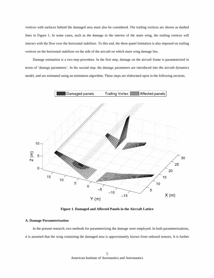
American Institute of Aeronautics and Astronautics
5
vortices with surfaces behind the damaged area must also be considered. The trailing vortices are shown as dashed
lines in Figure 1. In some cases, such as the damage in the interior of the main wing, the trailing vortices will
interact with the flow over the horizontal stabilizer. To this end, the three-panel limitation is also imposed on trailing
vortices on the horizontal stabilizer on the side of the aircraft on which main wing damage lies.
Damage estimation is a two-step procedure. In the first step, damage on the aircraft frame is parameterized in
terms of ‘damage parameters’. In the second step, the damage parameters are introduced into the aircraft dynamics
model, and are estimated using an estimation algorithm. These steps are elaborated upon in the following sections.
Figure 1. Damaged and Affected Panels in the Aircraft Lattice
A. Damage Parameterization
In the present research, two methods for parameterizing the damage were employed. In both parameterizations,
it is assumed that the wing containing the damaged area is approximately known from onboard sensors. It is further
American Institute of Aeronautics and Astronautics
6
assumed that damage only occurs on the edges of the wing. Hole-type damage in the wing was not considered in the
present research, although it can also be modeled using the proposed approach.
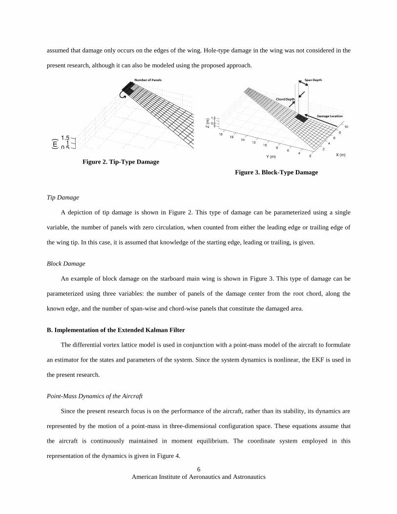
Figure 2. Tip-Type Damage
Figure 3. Block-Type Damage
Tip Damage
A depiction of tip damage is shown in Figure 2. This type of damage can be parameterized using a single
variable, the number of panels with zero circulation, when counted from either the leading edge or trailing edge of
the wing tip. In this case, it is assumed that knowledge of the starting edge, leading or trailing, is given.
Block Damage
An example of block damage on the starboard main wing is shown in Figure 3. This type of damage can be
parameterized using three variables: the number of panels of the damage center from the root chord, along the
known edge, and the number of span-wise and chord-wise panels that constitute the damaged area.
B. Implementation of the Extended Kalman Filter
The differential vortex lattice model is used in conjunction with a point-mass model of the aircraft to formulate
an estimator for the states and parameters of the system. Since the system dynamics is nonlinear, the EKF is used in
the present research.
Point-Mass Dynamics of the Aircraft
Since the present research focus is on the performance of the aircraft, rather than its stability, its dynamics are
represented by the motion of a point-mass in three-dimensional configuration space. These equations assume that
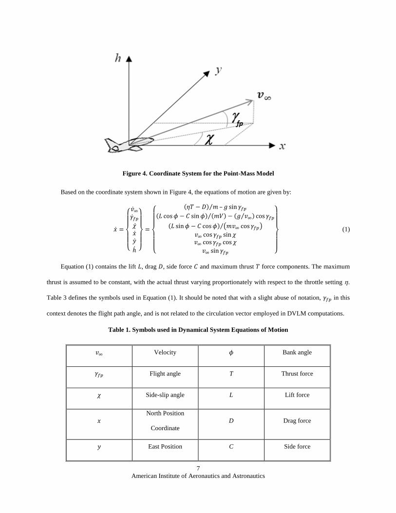
the aircraft is continuously maintained in moment equilibrium. The coordinate system employed in this
representation of the dynamics is given in Figure 4.
American Institute of Aeronautics and Astronautics
7
Figure 4. Coordinate System for the Point-Mass Model
Based on the coordinate system shown in Figure 4, the equations of motion are given by:
(1)
Equation (1) contains the lift , drag , side force and maximum thrust force components. The maximum
thrust is assumed to be constant, with the actual thrust varying proportionately with respect to the throttle setting .
Table 3 defines the symbols used in Equation (1). It should be noted that with a slight abuse of notation, in this
context denotes the flight path angle, and is not related to the circulation vector employed in DVLM computations.
Table 1. Symbols used in Dynamical System Equations of Motion
Velocity Bank angle
Flight angle T Thrust force
Side-slip angle L Lift force
North Position
Coordinate
D Drag force
East Position C Side force
American Institute of Aeronautics and Astronautics
8
Coordinate
Altitude M Mass
Throttle g
Acceleration due to
gravity
Evaluation of the Forces on an Impaired Aircraft using the DVLM
Under normal operating conditions, the lift, drag, and side force in Equation (1) can be expressed as functions
of aircraft wing area and aerodynamic parameters such as speed, angle of attack, and angle of sideslip.
In the case of physical damage to the airframe, such simple relationships may no longer be able to describe the
aerodynamic forces. The VLM allows the definition of the relationships between the airframe geometry and the
aerodynamic forces. The lift, drag, and side forces can be represented as the following nonlinear functions:
(2)
Here, is the air density, is the circulation distribution vector, is the aircraft geometry, is the in-flow speed,
is the angle of attack, and is the side-slip angle. However, in the conventional VLM, the dimension of is equal
to the number of panels approximating the airframe, normally a very large number. Designing estimators based on
the VLM is unrealistic due to its high dimension.
The DVLM calculates the differential circulation strength components in the vicinity of the damaged section
involving a much smaller set of circulation values in comparison with the conventional VLM approach. However, as
was shown in the previous work8,9
, the problem involves the estimation of several parameters, even with the use of
DVLM. Note that the parameterization of the damage can significantly reduce the dimension of the estimation
problem.
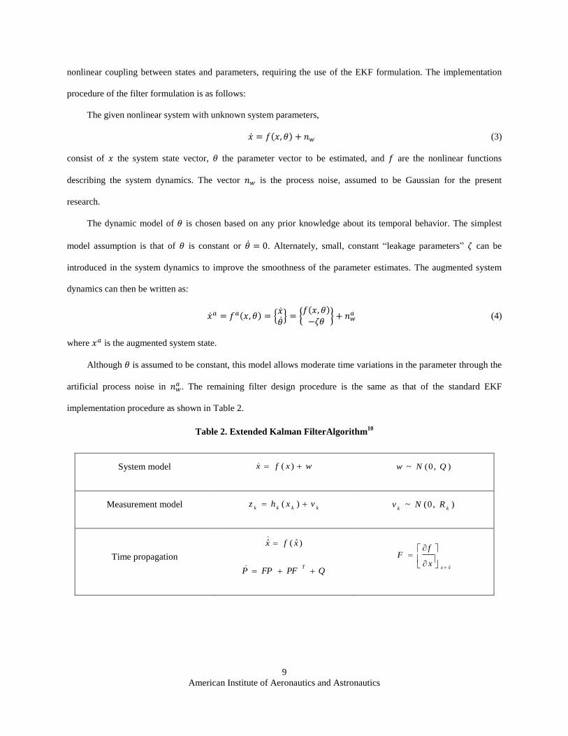
State-Parameter Estimation using the Extended Kalman Filter
The state-parameter estimation problem is often called the dual estimation problem since it requires
simultaneous estimation of the system states and unknown system parameters. In general, these problems involve
American Institute of Aeronautics and Astronautics
9
nonlinear coupling between states and parameters, requiring the use of the EKF formulation. The implementation
procedure of the filter formulation is as follows:
The given nonlinear system with unknown system parameters,
(3)
consist of the system state vector, the parameter vector to be estimated, and are the nonlinear functions
describing the system dynamics. The vector is the process noise, assumed to be Gaussian for the present
research.
The dynamic model of is chosen based on any prior knowledge about its temporal behavior. The simplest
model assumption is that of is constant or . Alternately, small, constant “leakage parameters” can be
introduced in the system dynamics to improve the smoothness of the parameter estimates. The augmented system
dynamics can then be written as:
(4)
where is the augmented system state.
Although is assumed to be constant, this model allows moderate time variations in the parameter through the
artificial process noise in . The remaining filter design procedure is the same as that of the standard EKF
implementation procedure as shown in Table 2.
Table 2. Extended Kalman FilterAlgorithm10
System model wxfx )(
),0(~ QNw
Measurement model
kkkkvxhz )(
),0(~
kkRNv
Time propagation
)ˆ(ˆ xfx
QPFFPPT
xx
x
fF
ˆ
American Institute of Aeronautics and Astronautics
10
Measurement update
)(ˆˆkkkkkk
xhzLxx
kkkkPHLIP )(
kxx
k
k
x
hH
ˆ
1
k
T
kkk
T
kkkRHPHHPL
For this state-parameter estimation problem, the measurements assumed to be available for the estimation
process are the three components of the position, velocity and acceleration vectors.
(5)
Here, is the measurement noise.
DVLM-based EKF Formulation
In the present research, the aerodynamic effects of airframe damage are directly estimated using the
parameterization methods described in the foregoing section. The filter directly estimates the actual size of the
damage using sensor measurements, and the DVLM algorithm provides circulation distribution solutions and the
resulting airframe pressure distribution and the forces. This approach has several advantages over the circulation
estimation approach demonstrated in References 8and 9. Firstly, the filter is robust to initialization errors and the
uncertainty in the initial damage estimate determined from sensors, since the damage size is directly estimated by
the filter. Secondly, damage parameterization generally involves a much smaller number of parameter states than the
number of circulation states, which will reduce the number of state variables to be estimated and thus improve the
observability of the system.
The major limitation of this damage estimation approach is that the DVLM module has to be executed at each
time step and sufficient accuracy is required for the DVLM solver since its output solution is directly used for the
subsequent force evaluation without being updated by sensor measurements.
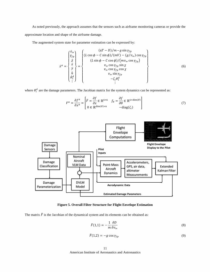
However, various numerical experiments during the present research revealed that the proposed DVLM
approach provides good accuracy and is computationally efficient, making it feasible to employ the current
estimation approach with direct damage parameterization. Figure 5 presents the structure of the estimator. In this
version, the filter incorporates sensor measurements with the estimated forces (i.e. lift, drag and side force) from the
DVLM solver to update the damage parameter states.
American Institute of Aeronautics and Astronautics
11
As noted previously, the approach assumes that the sensors such as airframe monitoring cameras or provide the
approximate location and shape of the airframe damage.
The augmented system state for parameter estimation can be expressed by:
(6)
where are the damage parameters. The Jacobian matrix for the system dynamics can be represented as:
(7)
Figure 5. Overall Filter Structure for Flight Envelope Estimation
The matrix is the Jacobian of the dynamical system and its elements can be obtained as:
(8)
(9)
Damage Sensors
DVLM Model
Damage Parameterization
Extended Kalman Filter
Point-Mass Aircraft
Dynamics
Damage Classification
Nominal Aircraft
VLM Data
FlightEnvelope
Computations
Pilot Inputs
Accelerometers, GPS, air data, altimeter Measurements
Flight Envelope Display to the Pilot
Estimated Damage Parameters
Aerodynamic Data
American Institute of Aeronautics and Astronautics
12
(10)
(11)
(12)
(13)
(14)
(15)
(16)
(17)
(18)
(19)
(20)
(21)
(22)
(23)
(24)
The function needs to be evaluated numerically due to the complexity of its functional representation. The
EKF has been programmed as a module together with the DVLM for the computation of aerodynamic forces, which
then form the basis for structural analysis and flight envelope computation modules.
Filter Initialization
As postulated at this juncture, the envelope estimation algorithm will be initialized as another avionics
component initialization during the pre-takeoff procedures, and will continue to operate throughout the flight
duration. In the absence of any damage, the filter will estimate the nominal values of the aerodynamic parameters.
American Institute of Aeronautics and Astronautics
13
If the aircraft structure experiences any structural damage, the filter will then proceed to estimate the parameters of
the impaired aircraft.
III. Inertial and Structural Characteristics of the Impaired Aircraft
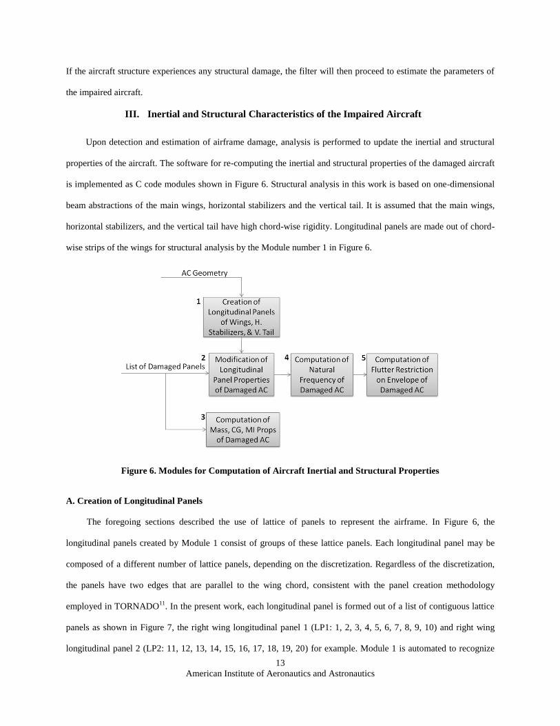
Upon detection and estimation of airframe damage, analysis is performed to update the inertial and structural
properties of the aircraft. The software for re-computing the inertial and structural properties of the damaged aircraft
is implemented as C code modules shown in Figure 6. Structural analysis in this work is based on one-dimensional
beam abstractions of the main wings, horizontal stabilizers and the vertical tail. It is assumed that the main wings,
horizontal stabilizers, and the vertical tail have high chord-wise rigidity. Longitudinal panels are made out of chord-
wise strips of the wings for structural analysis by the Module number 1 in Figure 6.
Figure 6. Modules for Computation of Aircraft Inertial and Structural Properties
A. Creation of Longitudinal Panels
The foregoing sections described the use of lattice of panels to represent the airframe. In Figure 6, the
longitudinal panels created by Module 1 consist of groups of these lattice panels. Each longitudinal panel may be
composed of a different number of lattice panels, depending on the discretization. Regardless of the discretization,
the panels have two edges that are parallel to the wing chord, consistent with the panel creation methodology
employed in TORNADO11
. In the present work, each longitudinal panel is formed out of a list of contiguous lattice
panels as shown in Figure 7, the right wing longitudinal panel 1 (LP1: 1, 2, 3, 4, 5, 6, 7, 8, 9, 10) and right wing
longitudinal panel 2 (LP2: 11, 12, 13, 14, 15, 16, 17, 18, 19, 20) for example. Module 1 is automated to recognize
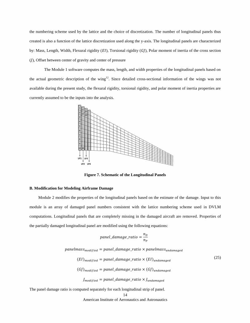
American Institute of Aeronautics and Astronautics
14
the numbering scheme used by the lattice and the choice of discretization. The number of longitudinal panels thus
created is also a function of the lattice discretization used along the y-axis. The longitudinal panels are characterized
by: Mass, Length, Width, Flexural rigidity ( ), Torsional rigidity ( ), Polar moment of inertia of the cross section
( ), Offset between center of gravity and center of pressure
The Module 1 software computes the mass, length, and width properties of the longitudinal panels based on
the actual geometric description of the wing12
. Since detailed cross-sectional information of the wings was not
available during the present study, the flexural rigidity, torsional rigidity, and polar moment of inertia properties are
currently assumed to be the inputs into the analysis.
Figure 7. Schematic of the Longitudinal Panels
B. Modification for Modeling Airframe Damage
Module 2 modifies the properties of the longitudinal panels based on the estimate of the damage. Input to this
module is an array of damaged panel numbers consistent with the lattice numbering scheme used in DVLM
computations. Longitudinal panels that are completely missing in the damaged aircraft are removed. Properties of
the partially damaged longitudinal panel are modified using the following equations:
(25)
The panel damage ratio is computed separately for each longitudinal strip of panel.
American Institute of Aeronautics and Astronautics
15
C. Computation of Mass, Center of Gravity, and Moment of Inertia
As a first step to the longitudinal panel computations in Module 1, the mass and centroid of individual lattice
panels are also computed. These form the basis for the update of the mass, center of gravity, and moment of inertia
properties of the damaged aircraft. The mass of the damaged panels is first set to zero. The center of gravity of the
damaged aircraft is then computed using the following equations:
(26)
The denominator on the right hand side of Equations (26) represents the mass of the damaged aircraft. The moment
of inertia of the damaged aircraft about the new center of gravity is computed as follows:
(27)
American Institute of Aeronautics and Astronautics
16
D. Computation of Structural Dynamic Frequencies
Every physical structure with mass and elasticity is capable of oscillatory motion and under certain conditions,
and can reach resonance under certain conditions. These natural frequencies are very important parameters in
structural system design and analysis.
Module 3 in Figure 6 computes the bending and torsional natural frequencies of the damaged aircraft
appendages (wings, horizontal stabilizers, and vertical tail) using the Holzer-Myklestad framework13,14
. The
computations of the bending and torsional frequencies are decoupled in the current approach. Bending frequencies
are expected to be used in determining the bandwidth of the inner-loop control system. Torsional frequencies form
the inputs to the module that computes the envelope restriction resulting from flutter.
Since the natural frequencies and the associated natural modes are inherent structural characteristics, they can
be determined once the layout of the structure and its material properties are given. However, the computational load
increases with the size and complexity of the structure. In the following section, an approximate, but efficient
method for calculating the natural modes and frequencies of the wing structure is formulated based on the lumped-
mass approximation.
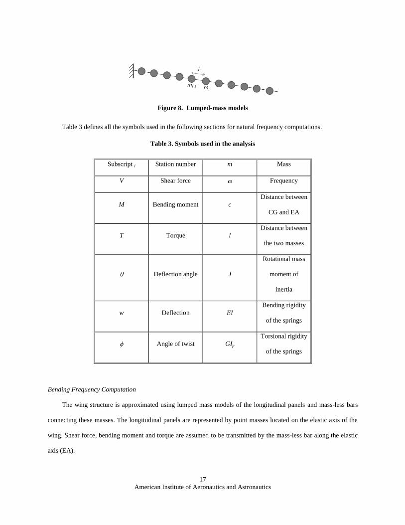
Lumped Mass Approximation
Ideally, structural analysis should be carried out with the structure being considered as a continuum. However,
such an analysis generally involves the solution of partial differential equations, necessitating advanced
computational algorithms. An approximate approach is to treat the structure as a set of lumped-masses connected
together by mass-less springs. These modes can provide very good estimates of the first few natural frequencies and
the associated natural modes, which are of practical importance in assessing structural safety. Figure 8 illustrates the
lumped-mass approximation of the aircraft wing employed in this work.
American Institute of Aeronautics and Astronautics
17
Figure 8. Lumped-mass models
Table 3 defines all the symbols used in the following sections for natural frequency computations.
Table 3. Symbols used in the analysis
Subscript i Station number m Mass
V Shear force Frequency
M Bending moment c
Distance between
CG and EA
T Torque l
Distance between
the two masses
Deflection angle J
Rotational mass
moment of
inertia
w Deflection EI
Bending rigidity
of the springs
Angle of twist GIp
Torsional rigidity
of the springs
Bending Frequency Computation
The wing structure is approximated using lumped mass models of the longitudinal panels and mass-less bars
connecting these masses. The longitudinal panels are represented by point masses located on the elastic axis of the
wing. Shear force, bending moment and torque are assumed to be transmitted by the mass-less bar along the elastic
axis (EA).
American Institute of Aeronautics and Astronautics
18
The Holzer-Myklestad method has proven useful and practical in the analyses of airplane wings13
. The
equation relating forces and displacement between two adjacent lumped mass stations can be represented as:
(28)
Equations (28) can be expressed as a transfer matrix as shown in the following equations, providing a more
effective and efficient representation for numerical computations:
(29)
Equations (29) can be applied from the free end ( ) to the fixed end ( ) to result in the following equation:
(30)
It should be noted that the Aij elements of the transfer function matrix in the above equation are functions of the
frequency. The following boundary conditions follow from the cantilever approximation of the appendages. All the
displacement at the fixed end must be zero and the shear force and bending moment must be zero at the free end.
(31)
Implementing the above boundary conditions in the last two rows of Equation (30) results in the following
condition:
(32)
A non-trivial solution to the above equations exists only if the determinant of the coefficient matrix on the right hand
side is zero. The Holzer-Mykelstad method computes natural frequencies as the frequency values that satisfy the
following equation:
American Institute of Aeronautics and Astronautics
19
(33)
Torsional Frequency Computation
The following equations are used for propagation of torque and twist through the lumped mass approximation:
(34)
Equations (34) can be expressed as a transfer matrix as shown in Equations (35), providing a more effective
and efficient representation for numerical computations.
(35)
Equations (35) can be applied from the free end ( ) to the fixed end ( ) to result in the following equation:
(36)
It should be noted that in the above equation are functions of the frequency . The following boundary
conditions follow from the cantilever approximation of the appendages. The twist at the fixed end must be zero, and
the torsion must be zero at the free end.
(37)
Substituting the above boundary conditions in Equation (36) results in the following condition:
(38)
Torsional frequencies are computed as solutions to the foregoing equation.
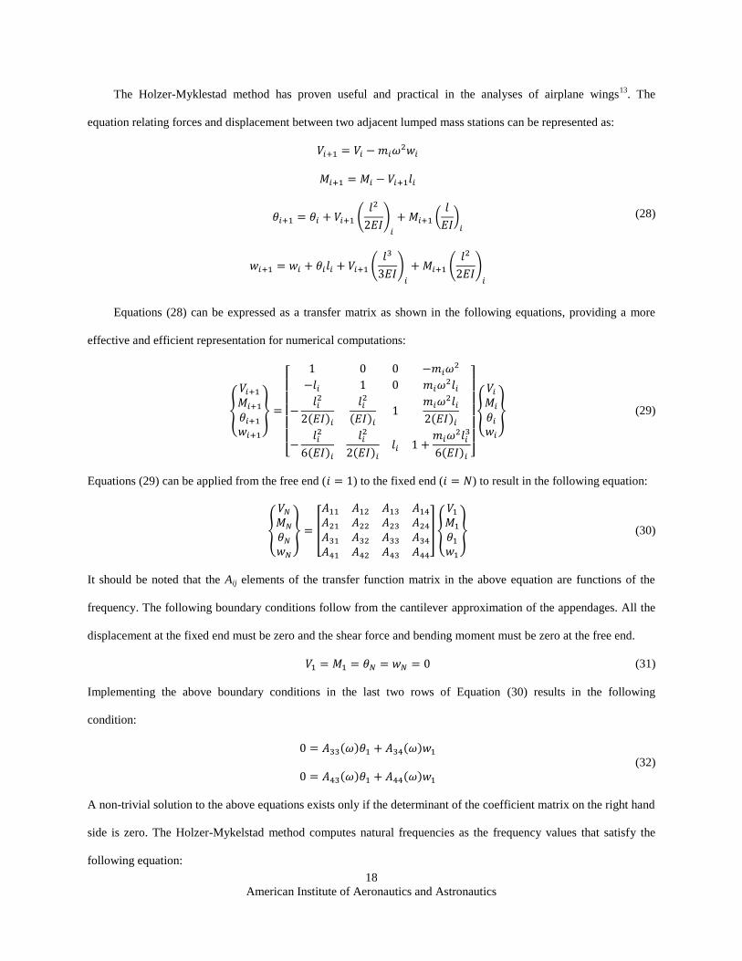
E. Computation of Wing Deflection
Airplane wings are designed to deflect substantially in flight under aerodynamic loading. Although the wings
only account for a portion of the overall aircraft weight they provide all the lift required to support the weight of the
aircraft. The pressure differential between lower and upper surfaces of the wing causes the wings to deflect upwards
during flight. In order to compute the deflection the wing, it is discretized by a series of longitudinal panels as
shown in Figure 9. The longitudinal discretization is motivated by the fact that the wings have high chord-wise
rigidity. Wing deflection due to bending is computed along the elastic axis of the wing. The wing weight is modeled
American Institute of Aeronautics and Astronautics
20
as uniformly distributed except for the engine weight which is modeled as a point force acting uniformly on one
complete panel.
Figure 9. Discretization of the Wing Using Longitudinal Panels
Li = Lift acting on the ith
longitudinal panel
Wi = Weight of the ith
longitudinal panel
Zi = (Li-Wi) Net vertical load on the ith
longitudinal panel
i = Width of the i
th longitudinal panel along the 'y axis
The first step in computing deflection due to bending is the computation of the bending moment which is
related to the shear stress distribution. The following equations are used to compute the shear stress and bending
moment respectively along the elastic axis of the wing14
, with zero shear stress and zero bending moment (
) boundary conditions being imposed at the free end of the wing.
(39)
Whereas the shear stress and bending moment are computed starting with the free end of the wing, the slope and
deflection of the wing are computed from the root of the wing with boundary conditions, , with the
following equations:
(40)
12 ith Longitudinal Panel
Elastic Axis
x
y
x’
y’i
Engine
American Institute of Aeronautics and Astronautics
21
F. Computation of Wing Torsion
In addition to bending, the aircraft wing also experiences torsion due to the chord-wise variation of lift.
Variation in lift results in a torque which causes the wing to twist about its torsional axis. The VLM computes the
lift on each sub-panel for a longitudinal panel. This, along with the geometric information about the panel can be
used to compute the chord-wise torque. The basic governing equation14
for torsional rotation is:
(41)
where is the torsional deflection, is the torque, and is the torsional rigidity that depends on the wing material
and the cross-sectional details. Coupling between bending and torsion is not modeled by this equation. The above
equation can be discretized as:
(42)
G. Wing Divergence Analysis
Aerodynamic pressure distributed on the wing surface induces a twisting moment in addition to bending
moments. These moments are resisted by the elastic restoring moment of the wing structure. While the aerodynamic
moment increases as the square of the flight speed, the structural stiffness remains unaltered. Hence, there exists a
critical speed at which the aerodynamic and elastic moments are in equilibrium. A structural instability called wing
divergence may occur at a speed higher than the critical speed. A simple two dimensional example is presented in
the following subsection to provide qualitative insight into this phenomenon. The analysis is then extended to a
cantilever wing structure.
The wing structure is simplified as a cantilever beam with a straight elastic axis perpendicular to the fuselage.
It is assumed that the wing is infinitely rigid in the chord-wise direction and the angle of twist varies only in the
span-wise direction. Both these assumptions are reasonable for conventional wings operating at low subsonic Mach
numbers.
American Institute of Aeronautics and Astronautics
22
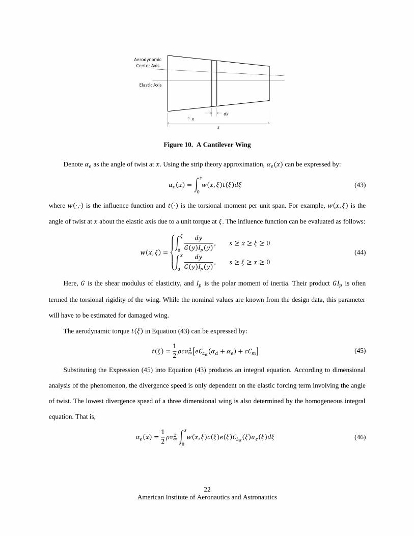
Figure 10. A Cantilever Wing
Denote as the angle of twist at . Using the strip theory approximation, can be expressed by:
(43)
where is the influence function and is the torsional moment per unit span. For example, is the
angle of twist at about the elastic axis due to a unit torque at . The influence function can be evaluated as follows:
(44)
Here, is the shear modulus of elasticity, and is the polar moment of inertia. Their product is often
termed the torsional rigidity of the wing. While the nominal values are known from the design data, this parameter
will have to be estimated for damaged wing.
The aerodynamic torque in Equation (43) can be expressed by:
(45)
Substituting the Expression (45) into Equation (43) produces an integral equation. According to dimensional
analysis of the phenomenon, the divergence speed is only dependent on the elastic forcing term involving the angle
of twist. The lowest divergence speed of a three dimensional wing is also determined by the homogeneous integral
equation. That is,
(46)
American Institute of Aeronautics and Astronautics
23
In general, closed form analytical solutions to Equation (46) are not available except for the simple case of a
rectangular wing with uniform chord and stiffness. For that case, Equation (46) can be rewritten as the following
differential equation.
(47)
Equation (47) is a linear differential equation, which can be solved for . Then, the lowest critical divergence
speed can then be obtained as 15
:
(48)
Numerical Solution to Wing Divergence
Since no closed-form solution is available in the general case, a numerical approach which can deal with a
more generalized wing configuration is employed in the present research. The approach is based on the lumped-
mass model, along the lines of the bending bar model described earlier in this in this section.
The 3-D wing structure is represented as a lumped-mass structure as shown in Figure 11. The integration in
Equation (47) is next represented as a summation over discretized wing segments.
(49)
where
(50)
American Institute of Aeronautics and Astronautics
24
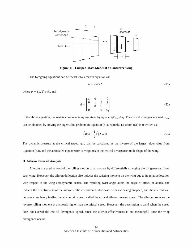
Figure 11. Lumped-Mass Model of a Cantilever Wing
The foregoing equations can be recast into a matrix equation as:
(51)
where , and
(52)
In the above equation, the matrix components are given by . The critical divergence speed,
can be obtained by solving the eigenvalue problem in Equation (51). Namely, Equation (51) is rewritten as:
(53)
The dynamic pressure at the critical speed, can be calculated as the inverse of the largest eigenvalue from
Equation (53), and the associated eigenvector corresponds to the critical divergence mode shape of the wing.
H. Aileron Reversal Analysis
Ailerons are used to control the rolling motion of an aircraft by differentially changing the lift generated from
each wing. However, the aileron deflection also induces the twisting moment on the wing due to its relative location
with respect to the wing aerodynamic center. The resulting twist angle alters the angle of attack of attack, and
reduces the effectiveness of the ailerons. The effectiveness decreases with increasing airspeed, and the ailerons can
become completely ineffective at a certain speed, called the critical aileron reversal speed. The aileron produces the
reverse rolling moment at airspeeds higher than the critical speed. However, the description is valid when the speed
does not exceed the critical divergence speed, since the aileron effectiveness is not meaningful once the wing
divergence occurs.
American Institute of Aeronautics and Astronautics
25
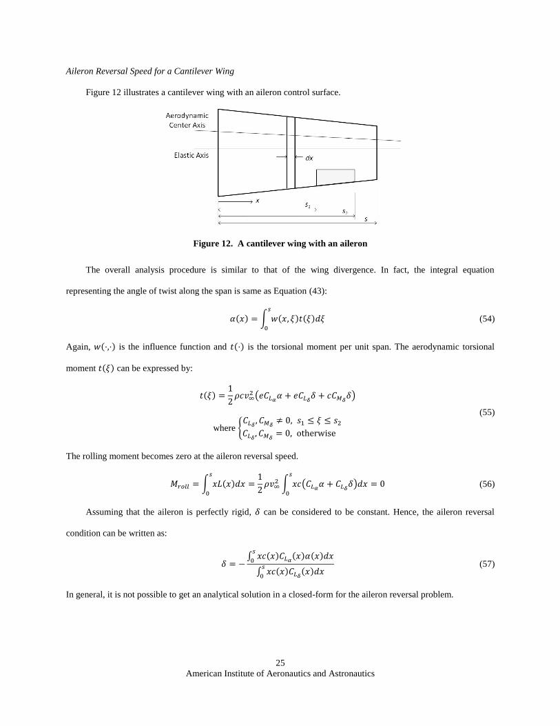
Aileron Reversal Speed for a Cantilever Wing
Figure 12 illustrates a cantilever wing with an aileron control surface.
Figure 12. A cantilever wing with an aileron
The overall analysis procedure is similar to that of the wing divergence. In fact, the integral equation
representing the angle of twist along the span is same as Equation (43):
(54)
Again, is the influence function and is the torsional moment per unit span. The aerodynamic torsional
moment can be expressed by:
where
(55)
The rolling moment becomes zero at the aileron reversal speed.
(56)
Assuming that the aileron is perfectly rigid, can be considered to be constant. Hence, the aileron reversal
condition can be written as:
(57)
In general, it is not possible to get an analytical solution in a closed-form for the aileron reversal problem.
American Institute of Aeronautics and Astronautics
26
Numerical Solution to the Aileron Reversal Speed Computation
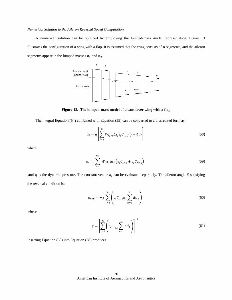
A numerical solution can be obtained by employing the lumped-mass model representation. Figure 13
illustrates the configuration of a wing with a flap. It is assumed that the wing consists of segments, and the aileron
segments appear in the lumped masses and .
Figure 13. The lumped-mass model of a cantilever wing with a flap
The integral Equation (54) combined with Equation (55) can be converted to a discretized form as:
(58)
where
(59)
and is the dynamic pressure. The constant vector can be evaluated separately. The aileron angle satisfying
the reversal condition is:
(60)
where
(61)
Inserting Equation (60) into Equation (58) produces
American Institute of Aeronautics and Astronautics
27
(62)
Equation (62) can be cast into a matrix equation as shown in the following.
(63)
Here, , , and are diagonal matrices. The diagonal elements in are , . Those in and are given
by the following:
(64)
The critical dynamic pressure, and the associated wing reversal speed, can be obtained by solving the
eigenvalue problem in Equation (63). As in the case of wing divergence, the torsional stiffness of the damaged wing
is required for the calculation of aileron reversal.
I. Flutter Analysis
Flutter is a dynamic aeroelastic phenomenon, and its rigorous treatment is known to be extremely challenging.
In present study, a relatively simple approach to estimate flutter conditions is proposed assuming that relative flutter
criteria for an undamaged aircraft are available in advance.
Basic Approach to Flutter
Flutter is a complex aeroelastic phenomenon. Although large body of research exists, it remains an active area
of research. The key objective of the flutter analysis in the present study is to provide a safe and conservative
boundary for a damaged aircraft using limited information on the structural damage. One of the fundamental
requirements of the present flutter boundary estimation is that it should be simple enough for real-time
computations. Existing flutter estimation techniques are based on wind-tunnel experiments or uses computationally
intensive algorithms, which are not suitable for the current application.
American Institute of Aeronautics and Astronautics
28
Instead, a simple closed-form formula which provides an approximate flutter condition is advanced. This
formula utilizes the results from the natural frequency/mode analysis discussed in an earlier section, along with prior
available information on flutter criteria of the undamaged aircraft.
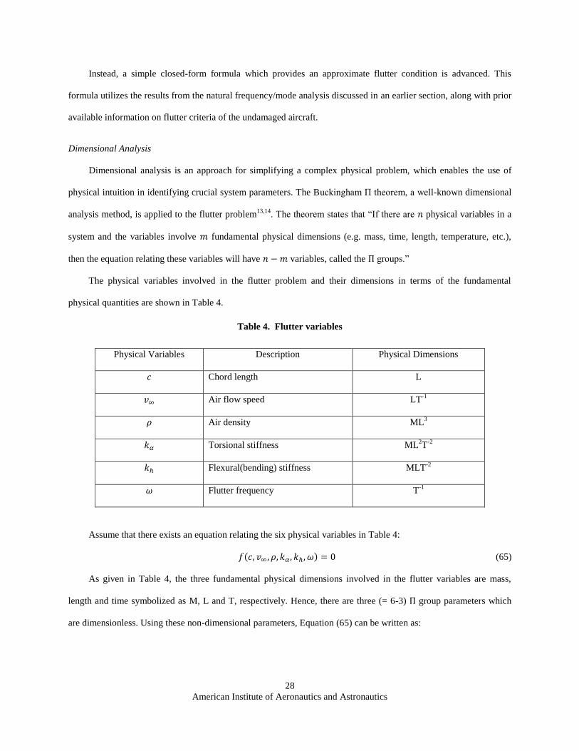
Dimensional Analysis
Dimensional analysis is an approach for simplifying a complex physical problem, which enables the use of
physical intuition in identifying crucial system parameters. The Buckingham Π theorem, a well-known dimensional
analysis method, is applied to the flutter problem13,14
. The theorem states that “If there are physical variables in a
system and the variables involve fundamental physical dimensions (e.g. mass, time, length, temperature, etc.),
then the equation relating these variables will have variables, called the groups.”
The physical variables involved in the flutter problem and their dimensions in terms of the fundamental
physical quantities are shown in Table 4.
Table 4. Flutter variables
Physical Variables Description Physical Dimensions
Chord length L
Air flow speed LT-1
Air density ML3
Torsional stiffness ML2T
-2
Flexural(bending) stiffness MLT-2
Flutter frequency T-1
Assume that there exists an equation relating the six physical variables in Table 4:
(65)
As given in Table 4, the three fundamental physical dimensions involved in the flutter variables are mass,
length and time symbolized as M, L and T, respectively. Hence, there are three (= 6-3) group parameters which
are dimensionless. Using these non-dimensional parameters, Equation (65) can be written as:
American Institute of Aeronautics and Astronautics
29
(66)
This functional relationship expresses the dynamic similitude condition. The first parameter, , is called
the reduced frequency or Strouhal number, abbreviated as , which is perhaps the most important parameter
describing oscillating motion in unsteady fluid flow. In fact, the remaining parameters, and , are also related to
the Strouhal number: they can be identified with the square of the Strouhal number.
It can be assumed that the flutter speed can be efficiently estimated by exploiting the relationship between the
physical variables.
Flutter Criteria
A simple formula based on the Strouhal number which gives the critical flutter speed can be expressed as14
:
(67)
The aircraft speed must be lower than to avoid flutter. Here, is the chord length, and is the
fundamental frequency of the wing in the torsional vibration mode. is the critical Strouhal number at which
flutter occurs. The range of is dependent on various parameters such as design specifications and structural
properties. Every aircraft design is subject to rigorous flutter analysis. Thus, the flutter-related parameters including
the critical Strouhal number in Equation (67) are generally available for undamaged aircraft beforehand.
If it can be assumed that the critical Strouhal number for the undamaged aircraft is valid for the same aircraft
with known structure damage, the critical flutter speed can be determined by plugging and of the damaged
aircraft into Equation (67). For example, if the wing is damaged, its effective chord length will be reduced, and
will also be decreased due to the reduction in structural stiffness, which results in the decrease of .
Also, Equation (66) shows two additional non-dimensional parameters, and . The same procedure
described above can be applied to these parameters as well. More conservative flutter criteria can be provided by
considering all these non-dimensional parameters. That is, can be evaluated for all three non-dimensional
parameters, and the smallest of the three can then be used as the critical flutter speed.
American Institute of Aeronautics and Astronautics
30
IV. Impaired Aircraft Flight Envelope
The flight envelope defines the extreme conditions at which steady flight can maintained. Aircraft flight
envelope is estimated by trimming the estimated model of the aircraft at various flight conditions, and then
determining the envelope of the trim set. Since the low-speed part of the flight envelope is mainly determined by
aircraft stall angle of attack, the following section will provide some details on the approach adopted in the present
paper.
A. Stall Angle of Attack Computation
Stall can be qualitatively defined as abrupt loss of lift accompanied by degraded control surface effectiveness
as the angle of attack is increased. The angle of attack associated with the maximum lift coefficient is termed as the
maximum allowable angle of attack. The lift decreases rapidly beyond this angle of attack. Therefore, to predict
stall, it is important to be able to predict the functional relationship between angle of attack and the coefficient of
lift. The maximum lift coefficient determines the minimum airspeed at which the aircraft can develop enough lift to
sustain its weight, and consequently defines the stall speed.
Stall is caused due to viscous boundary layer16
effects such as flow separation. Therefore, inviscid flow solvers
such as vortex lattice method and the differential vortex lattice method cannot capture this phenomenon. Wind-
tunnel testing using scale models17,18
appears to be one of the reliable methods for the prediction of stall conditions.
The second option involves solving the complete Navier-Stokes equation using advanced numerical techniques19,20
.
Neither of these is feasible for onboard use in impaired aircraft.
Approximate computational techniques that do not involve the solution of the full-fledged Navier-Stokes
equation have been considered in References 21-28. Some of these works21-24
are limited to 2-D airfoil stall
prediction and hence not suitable for recalculating the stall conditions for an aircraft with wing-tip damage. Three
dimensional numerical approaches for computing the aerodynamic coefficients are presented in References 25 and
28. These approaches are iterative in nature involving a 3-D inviscid solver such as the vortex lattice method
boundary layer solvers. Reference 25 adopts 3-D vortex lattice method and 2-D boundary layer solvers based on the
developments from References 26 and 27. Iterations involve flow field computation using the 3-D inviscid solver,
and computation of the boundary layer displacement thickness using the 2-D boundary layer solver. The
displacement thickness obtained from the boundary layer solver is added to the airfoil geometry and a new camber
American Institute of Aeronautics and Astronautics
31
line is obtained. In the next iteration VLM computations are done using the modified airfoil geometry and the
process is continued until changes observed in the lift coefficients fall below a specified tolerance. Reference 28
uses a 3-D inviscid solver and 3D boundary layer solution for aerodynamic coefficient computation and hence can
be expected to be able to handle stall prediction for an aircraft with wing-tip damage. The methodology adopted in
this work is referred to as “Interactive Boundary Layer Method (IBLM)” and is even suitable for multi-element
airfoils. The approach is shown in Reference 28 to be suitable for stall and post-stall computations.
Even though the approaches presented in References 25 and 28 are not as computationally intensive as the
Navier-Stokes CFD method, they still involve considerable computational effort. Both these approaches are iterative
in nature and involve the vortex lattice solution in every iteration. Therefore, alternatives involving a combination of
modeling approximations and new implementation architectures are required to facilitate the online implementation
of the methods presented in References 25 and 28.
In the present research, the procedure of obtaining for a finite wing from Reference 15 is employed for
deriving an approximate stall angle of attack for the impaired aircraft. In Reference 15, the maximal lift coefficient
of the finite wing is obtained by considering span-wise load distribution, which is specified by the local lift
coefficient. In other words, the maximal lift coefficient of the finite wing is obtained as the lift coefficient at
which a local lift coefficient reaches the maximal 2-D lift coefficient . The maximal 2-D lift coefficient
is available from the standard airfoil database, which has been determined from multiple wind tunnel tests29
. Since
the air flow separation at a local strip does not necessarily decrease the total lift generated by the entire wing, the
derived using this procedure tends to be conservative. However, this approach allows for a quantitative
estimate for the stall angle of attack for the damaged wing without resorting to a complex CFD solution.
In the present research, the stall angle of attack is derived following the approach presented in Reference 15.
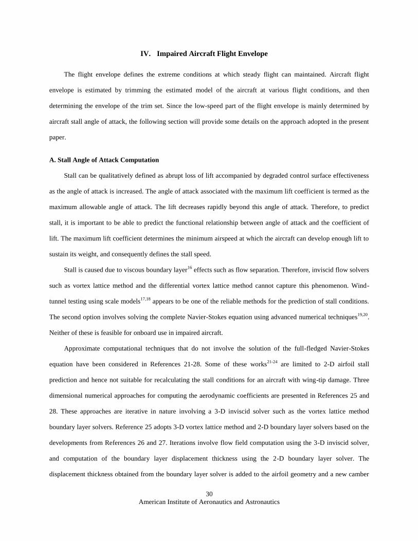
Consider the local longitudinal strip depicted in Figure 14. The local lift coefficient for the longitudinal strip is
defined as
(68)
where is the lift on the strip, is the area of the strip, and
is the dynamic pressure, where is
the air density, and is the air speed. The maximal strip lift coefficient for the entire wing is defined as the
maximum of the local lift coefficients of longitudinal strips in the wing, i.e.,
American Institute of Aeronautics and Astronautics
32
(69)
where the angle of attack is introduced to show the dependency of the maximal local lift coefficient to the angle of
attack.
Figure 14. Illustration of a Longitudinal Strip on a Wing
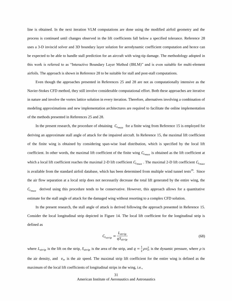
Then, the stall angle of attack for the damaged wing is obtained as the angle of attack which leads to the
maximal local lift coefficient which matches of the nominal undamaged wing at the known stall angle of
attack, in the current implementation. In other words, the stall angle of attack is given by
(70)
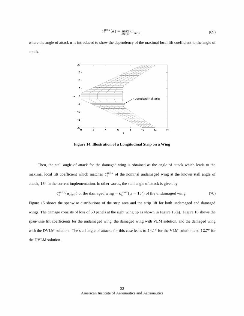
Figure 15 shows the spanwise distributions of the strip area and the strip lift for both undamaged and damaged
wings. The damage consists of loss of 50 panels at the right wing tip as shown in Figure 15(a). Figure 16 shows the
span-wise lift coefficients for the undamaged wing, the damaged wing with VLM solution, and the damaged wing
with the DVLM solution. The stall angle of attacks for this case leads to for the VLM solution and for
the DVLM solution.
American Institute of Aeronautics and Astronautics
33
(a) Strip area
(b) Strip lift
Figure 15. Area and Lift Distributions for the Wing-Tip Damage
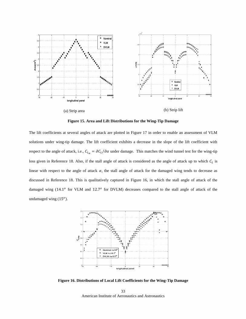
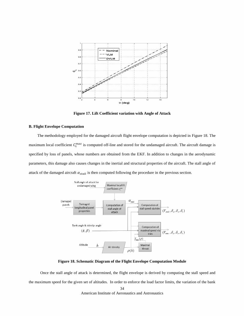
The lift coefficients at several angles of attack are plotted in Figure 17 in order to enable an assessment of VLM
solutions under wing-tip damage. The lift coefficient exhibits a decrease in the slope of the lift coefficient with
respect to the angle of attack, i.e., under damage. This matches the wind tunnel test for the wing-tip
loss given in Reference 18. Also, if the stall angle of attack is considered as the angle of attack up to which is
linear with respect to the angle of attack , the stall angle of attack for the damaged wing tends to decrease as
discussed in Reference 18. This is qualitatively captured in Figure 16, in which the stall angle of attack of the
damaged wing ( for VLM and for DVLM) decreases compared to the stall angle of attack of the
undamaged wing ( .
Figure 16. Distributions of Local Lift Coefficients for the Wing-Tip Damage
American Institute of Aeronautics and Astronautics
34
Figure 17. Lift Coefficient variation with Angle of Attack
B. Flight Envelope Computation
The methodology employed for the damaged aircraft flight envelope computation is depicted in Figure 18. The
maximum local coefficient is computed off-line and stored for the undamaged aircraft. The aircraft damage is
specified by loss of panels, whose numbers are obtained from the EKF. In addition to changes in the aerodynamic
parameters, this damage also causes changes in the inertial and structural properties of the aircraft. The stall angle of
attack of the damaged aircraft is then computed following the procedure in the previous section.
Figure 18. Schematic Diagram of the Flight Envelope Computation Module
Once the stall angle of attack is determined, the flight envelope is derived by computing the stall speed and
the maximum speed for the given set of altitudes. In order to enforce the load factor limits, the variation of the bank
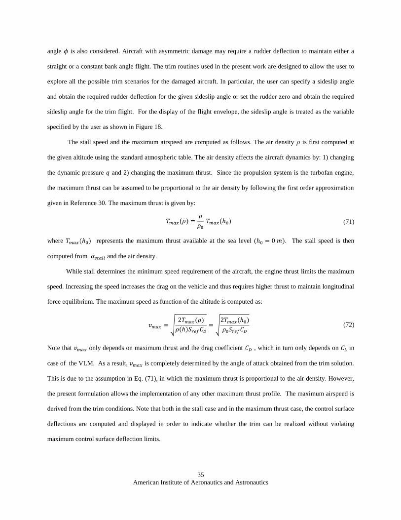
American Institute of Aeronautics and Astronautics
35
angle is also considered. Aircraft with asymmetric damage may require a rudder deflection to maintain either a
straight or a constant bank angle flight. The trim routines used in the present work are designed to allow the user to
explore all the possible trim scenarios for the damaged aircraft. In particular, the user can specify a sideslip angle
and obtain the required rudder deflection for the given sideslip angle or set the rudder zero and obtain the required
sideslip angle for the trim flight. For the display of the flight envelope, the sideslip angle is treated as the variable
specified by the user as shown in Figure 18.
The stall speed and the maximum airspeed are computed as follows. The air density is first computed at
the given altitude using the standard atmospheric table. The air density affects the aircraft dynamics by: 1) changing
the dynamic pressure and 2) changing the maximum thrust. Since the propulsion system is the turbofan engine,
the maximum thrust can be assumed to be proportional to the air density by following the first order approximation
given in Reference 30. The maximum thrust is given by:
(71)
where represents the maximum thrust available at the sea level ( . The stall speed is then
computed from and the air density.
While stall determines the minimum speed requirement of the aircraft, the engine thrust limits the maximum
speed. Increasing the speed increases the drag on the vehicle and thus requires higher thrust to maintain longitudinal
force equilibrium. The maximum speed as function of the altitude is computed as:
(72)
Note that only depends on maximum thrust and the drag coefficient , which in turn only depends on in
case of the VLM. As a result, is completely determined by the angle of attack obtained from the trim solution.
This is due to the assumption in Eq. (71), in which the maximum thrust is proportional to the air density. However,
the present formulation allows the implementation of any other maximum thrust profile. The maximum airspeed is
derived from the trim conditions. Note that both in the stall case and in the maximum thrust case, the control surface
deflections are computed and displayed in order to indicate whether the trim can be realized without violating
maximum control surface deflection limits.
American Institute of Aeronautics and Astronautics
36
C. Flight Deck Display of Aircraft Impairment and the Flight Envelope
As discussed in the Introduction, it is assumed that an adaptive stabilization system2-4
continues to maintain the
aircraft at its current flight conditions. The flight envelope computation algorithms discussed in the foregoing
sections then generate the data for display to the pilot.
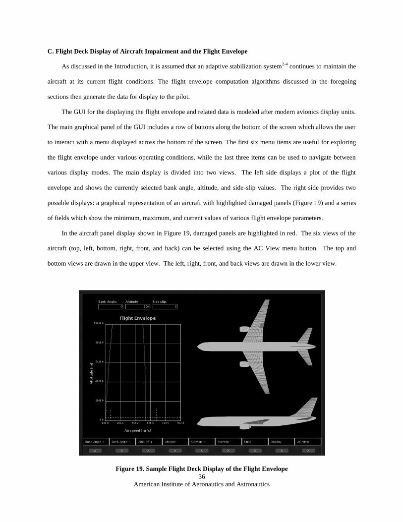
The GUI for the displaying the flight envelope and related data is modeled after modern avionics display units.
The main graphical panel of the GUI includes a row of buttons along the bottom of the screen which allows the user
to interact with a menu displayed across the bottom of the screen. The first six menu items are useful for exploring
the flight envelope under various operating conditions, while the last three items can be used to navigate between
various display modes. The main display is divided into two views. The left side displays a plot of the flight
envelope and shows the currently selected bank angle, altitude, and side-slip values. The right side provides two
possible displays: a graphical representation of an aircraft with highlighted damaged panels (Figure 19) and a series
of fields which show the minimum, maximum, and current values of various flight envelope parameters.
In the aircraft panel display shown in Figure 19, damaged panels are highlighted in red. The six views of the
aircraft (top, left, bottom, right, front, and back) can be selected using the AC View menu button. The top and
bottom views are drawn in the upper view. The left, right, front, and back views are drawn in the lower view.
Figure 19. Sample Flight Deck Display of the Flight Envelope
American Institute of Aeronautics and Astronautics
37
V. Conclusions
The present research was motivated by the desirability of relating the impaired aircraft geometry with its flight
dynamics. Central premises involved in the research were that the inner-loop flight control system allows the
continued flight of the aircraft, onboard sensors such as electro-optical sensors can provide information about the
location of the damage on the airframe, and that the Vortex Lattice method can provide sufficiently accurate
aerodynamic characterization of the aircraft. The focus of the work was on a near real-time assessment of the effect
of damage on the aircraft flight envelope based on a differential formulation Vortex Lattice Method, combined with
an Extended Kalman Filter. The implementation has resulted in a full-scale GUI-based software package that can be
integrated with present-day avionics systems. The accomplishments of the present research are:
1. Full-scale implementation of the DVLM and EKF algorithms, and demonstration of damage estimation
process on realistic aircraft model. This research has demonstrated that it is feasible to rapidly estimate the
aerodynamic performance of damaged aircraft.
2. The aerodynamic data derived from the DVLM-EKF algorithm was used to calculate the effects of damage
on structural deflections, and the structural dynamics of the aircraft.
3. The data from the forgoing algorithms were used to compute the flight and maneuver envelopes, and can
form the basis for deriving safe guidance strategies for landing the aircraft. A sample avionics display to
the aid the pilot in managing the damage was developed based on these estimates. This display can assist
the pilot in planning safe trajectories for landing the damaged aircraft.
DVLM methodology invented under the present research combined with the EKF algorithm can be highly
effective in managing the effects of damage on an aircraft. The proposed methodology can be extended to estimate
more detailed aerodynamic data, and use them for enhancing the inner-loop autopilot. Other enhancements to the
present methodology may include the estimation of ground effects on the damaged aircraft. These and other issues
will be of future interest.
Acknowledgments
This research was supported by NASA Contract No. NNX09CA01C with Ms. Diana M. Acosta serving as the
Technical Monitor. The authors thank Ms. Acosta, Dr. Nhan Nguyen, Dr. K. Krishnakumar and Mr. John
Kaneshige for their enthusiasm and support of this work.
American Institute of Aeronautics and Astronautics
38
References
1http://www.aeronautics.nasa.gov/nra_pdf/irac_tech_plan_c1.pdf.
2Nguyen, N., Krishnakumar, K., Kaneshige, J., and Nespeca, P., “Dynamics and Adaptive Control for Stability Recovery of
Damaged Asymmetric Aircraft,” AIAA Guidance, Navigation, and Control Conference, Keystone, CO, Paper AIAA 2006-6049,
Aug. 2006.
3Nguyen, N., Krishnakumar, K., Kaneshige, J., and Nespeca, P., “Flight Dynamics and Hybrid Adaptive Control for Stability
Recovery of Damaged Asymmetric Aircraft,” Journal of Guidance, Control, and Dynamics, Vol. 31, No. 3, pp. 751-764, May-
Jun. 2008.
4Rysdyk, R.T., and Calise, A. J., “Fault Tolerant Flight Control via Adaptive Neural Network Augmentation,” AIAA
Guidance, Navigation, and Control Conference, Boston, MA, Paper AIAA-1998-4483, Aug. 1998.
5Menon, P. K., Vaddi, S. S., and Sengupta, P., "Robust Landing Guidance Law for Impaired Aircraft." AIAA Guidance,
Navigation, and Control Conference, Paper AIAA-2010-7702 , August 2 - 5, 2010, Toronto, Canada; to appear in the Journal of
Guidance, Control, and Dynamics.
6Astrom, K. J., and Wittenmark, B., Adaptive Control, Addison-Wesley, Menlo Park, CA, 1989.
7Moran, J., An Introduction to Theoretical and Computational Aerodynamics, John Wiley & Sons, Inc., New York, NY,
1984.
8Menon, P. K., Palaniappan, K., and Kim, J., "Rapid Estimation of Aircraft Performance Models using Differential Vortex
Panel Method and Extended Kalman Filter," Final Report prepared under NASA Phase I SBIR Contract No. NNX08CA50P,
Optimal Synthesis Inc., Los Altos, CA, July 21, 2008.
9Kim, J., Palaniappan, K., and Menon, P. K., "Rapid Estimation of Impaired Aircraft Aerodynamic Parameters," Journal of
Aircraft, Vol. 47, No. 4, July-August 2010, pp. 1216-1228.
10Gelb, A., Applied Optimal Estimation, M.I.T. Press, 1979.
11Melin, T., “A Vortex Lattice MATLAB Implementation for Linear Aerodynamic Wing Applications,” Master of
Engineering Thesis, Royal Institute of Technology, Sweden, Dec. 2000.
12http://www.boeing.com/commercial/airports/acaps/757_23.pdf.
13Thomson, W. T., Theory of Vibration with Applications, Prentice-Hall, Inc., Englewood Cliffs, NJ, 1988.
14Fung, Y. C., An Introduction to the Theory of Aeroelasticity, Dover Publications, Inc., Mineola, NY, 1993.
15McCormick, B.W., Aerodynamics, Aeronautics, and Flight Mechanics, John Wiley and Sons, 1979.
16White, F. M., Viscous Fluid Flow, McGraw Hill International Edition., Mineola, NY, 1993.
17Reilly, D. N., "A Useful Method of Airfoil Stall Prediction," Journal of Aircraft, Vol. 4, No. 6.
American Institute of Aeronautics and Astronautics
39
18Shah, G. H., "Aerodynamic Effects and Modeling of Damage to Transport Aircraft," Proceedings of the AIAA Guidance,
Navigation, Control Conference and Exhibit, Honolulu, HW, August 2008.
19Shelton, A., Abras, J., Jurenko, R., and Smith, M. J., "Improving the CFD Predictions of Airfoils in Stall," Proceedings of
the 43rd Aerospace Sciences Meeting & Exhibit, Reno, NV, January 2005.
20Davidson, L., and Rizzi, A., "Navier-Stokes Stall Predictions Using an Algebraic Reynolds-Stress Model," Journal of
Spacecraft and Rockets, Vol. 26, No. 6, Nov-Dec 1992.
21Herring, R. N., and Ely, W., "Laminar Leading Edge Stall Prediction for Thin Airfoils," Proceedings of the 11th AIAA Fluid
and Plasma Dynamics Conference, Seattle, WA, July 1978.
22Goradia, S. H., and Lyman, V., "Laminar Stall Prediction and Estimation of CL(max)," Journal of Aircraft, Vol. 11, No. 9.
23Blascovich, J. D., "Characteristics of Separated Flow Airfoil Analysis Methods," Proceedings of the 22nd AIAA Aerospace
Sciences Meeting, Reno, NV, January 1984.
24Blascovich, J. D., "A Comparison of Separated Flow Airfoil Analysis Methods," Journal of Aircraft, Vol. 22, No. 3.
25Lupo, S., Nyberg, H., Karlsson, A., and Mosheni, K., "Xwing – A 3D Viscous Design Tool for Wings," Proceedings of the
46th Aerospace Sciences Meeting & Exhibit, Reno, NV, January 2008.
26Drela, M., "Newton Solution of Coupled Viscous/Inviscid Multi-element Airfoil Flows," Proceedings of the 21st AIAA
Fluid Dynamics, Plasma Dynamics and Lasers Conference, Seattle, WA, June 1990.
27Drela, M., and Giles, M., "Viscous-Inviscid Analysis of Transonic and Low Reynolds Number Airfoils," AIAA Journal,
Vol. 25, No. 10.
28Besnard, E., Puech, B., Ivshin, D., Kural, O., and Cebeci, T., "Prediction of Stall and Post-Stall in Two and Three-
Dimensional Flows," Proceedings of the 38th Aerospace Sciences Meeting & Exhibit, Reno, NV, January 2000.
29Raymer, P. D., Aircraft Design:A Conceptual Approach, AIAA Education Series, 1992.
30Anderson, J. D., Introduction to Flight, Mcgraw-Hill,1989.