Imperfect Inspection of a System With Unrevealed Failure

Imperfect inspection of a system withunrevealed failure and an unrevealed

defective stateCavalcante, C, Scarf, PA and Berrade, MD

http://dx.doi.org/10.1109/TR.2019.2897048

Title Imperfect inspection of a system with unrevealed failure and an unrevealeddefective state

Authors Cavalcante, C, Scarf, PA and Berrade, MD

Type Article

URL This version is available at: http://usir.salford.ac.uk/id/eprint/49849/

Published Date 2019

USIR is a digital collection of the research output of the University of Salford. Where copyright permits, full text material held in the repository is made freely available online and can be read, downloaded and copied for non-commercial private study or research purposes. Please check the manuscript for any further copyright restrictions.

For more information, including our policy and submission procedure, pleasecontact the Repository Team at: [email protected].

mailto:[email protected]

This article has been accepted for inclusion in a future issue of this journal. Content is final as presented, with the exception of pagination.

IEEE TRANSACTIONS ON RELIABILITY 1

Imperfect Inspection of a System With UnrevealedFailure and an Unrevealed Defective State

Cristiano A. V. Cavalcante, Philip A. Scarf , and M. D. Berrade

Abstract—This paper proposes a model of inspection of a pro-tection system in which the inspection outcome provides imperfectinformation of the state of the system. The system itself is requiredto operate on demand typically in emergency situations. The pur-pose of inspection is to determine the functional state of the systemand consequently whether the system requires replacement. Thesystem state is modeled using the delay time concept in which thefailed state is preceded by a defective state. Imperfect inspectionis quantified by a set of probabilities that relate the system stateto the outcome of the inspection. The paper studies the effect ofthese probabilities on the efficacy of inspection. The analysis indi-cates that preventive replacement mitigates low-quality inspectionand that inspection is cost-effective provided the imperfect inspec-tion probabilities are not too large. Some derivative policies inwhich replacement is “postponed” following a positive inspectionare also studied. An isolation valve in a utility network motivates themodeling.

Index Terms—Delay-time model, preventive maintenance,protection system, quality of service, replacement.

NOTATION

T, T∗ Inspection interval (a decision variable) and itsoptimum value.

M, M∗ Number of inspections until preventive replacement(a decision variable) and its optimum value.

X System age at defect arrival with s-density,s-distribution, and reliability functions fX , FX , FX .

Y Delay-time from defect arrival to subsequent failure(time in defective state) with s-density, s-distribution,and reliability functions fY , FY , FY .

G, D, F System states: good, defective, failed, respectively.P, N Inspection outcomes: positive, negative.α Imperfect inspection probability Pr(P|G).β1 Imperfect inspection probability Pr(N|D).

Manuscript received February 3, 2018; revised June 4, 2018 and November27, 2018; accepted January 22, 2019. Date of publication; date of current version.The work of M. D. Berrade was supported by the Spanish Ministry of Economyand Competitiveness under Project MTM2015-63978-P. The work of C. A. V.Cavalcante was supported by CNPq (Brazilian Research Council). AssociateEditor: B. Xu. (Corresponding author: Philip A. Scarf.)

C. A. V. Cavalcante is with the Department of Engineering Management, Uni-versidade Federal de Pernambuco, Recife 50740-550, Brazil (e-mail:,[email protected]).

P. A. Scarf is with the Salford Business School, University of Salford, M54WT Manchester, U.K. (e-mail:,[email protected]).

M. D. Berrade is with the Department of Statistics, Universidad de Zaragoza,50018 Zaragoza, Spain (e-mail:,[email protected]).

Color versions of one or more of the figures in this paper are available onlineat http://ieeexplore.ieee.org

Digital Object Identifier 10.1109/TR.2019.2897048

β2 Imperfect inspection probability Pr(N|F).λ Mean of exponential delay-time distribution.γ Characteristic life parameter of Weibull defect arrival

distribution.δ Shape parameter of Weibull defect arrival distribution.cI Cost of an inspection.cR Cost of a replacement.cF Downtime cost-rate.U Cost of a renewal cycle.W Downtime in a renewal cycle.V Length of a renewal cycle.Q Long-run total cost per unit time, cost-rate (objective

function).

I. INTRODUCTION

THIS PAPER studies a protection or preparedness systemsubject to imperfect inspection. This system is required

to operate on demand typically in emergency situations. Suchprotection systems include military defense systems, medicalequipment (e.g., defibrillators), automobile airbags, isolationvalves, fire suppressors and alarms, secondary power supplies,and flood defenses. The Thames barrier [1] is an example ofthe latter. If this system fails to operate when the water level ofthe river is predicted to flood London, then estimates of the costof such a failure are tens of billions of pounds. These systemsare inspected or tested on a regular basis to determine theirfunctional state. Thus, isolation valves are closed and opened,cold-standby pumps are started, and the Thames barrier is raised.Such “inspections” incur significant costs. Therefore, systemowners wish to know how often inspections should be performedand whether inspection is effective.

In the proposed model, inspection is imperfect, so that thetrue functional state of the system cannot be known with cer-tainty. The efficacy of inspection is then suspect, and there mayexist circumstances in which inspection is not sufficiently ef-fective to be economically justified. Such imperfect testing hasbeen considered for critical systems [2]–[4] and for protectionsystems [5], [6]. These latter works are extended in this paperby supposing that a protection system is subject to a three-state failure process and inspection is imperfect. In the three-state failure process, a failure is preceded by the defective stateand sojourns in the good and defective states are random vari-ables [7], [8]. This is the delay-time concept, developed initiallyby Christer [9], and later extended by many others for pro-tection systems [3], [6]–[8], [10], [11] and for critical systems

This work is licensed under a Creative Commons Attribution 3.0 License. For more information, see http://creativecommons.org/licenses/by/3.0/

https://orcid.org/0000-0001-5623-906X






2 IEEE TRANSACTIONS ON RELIABILITY

[12]–[17]. The sojourn in defective state is the delay-time. Fora critical system, failure is self-announcing and the object ofinspection is failure prevention. For a protection system, failureis not self-announcing and the object of inspection is to revealthe functional state of the system—that is, to determine whetherthe protection system will operate in the event of a demand forits function.

Others have extended the delay-time concept to critical sys-tems with minor and major defect states, to model real systemsmore closely. However, imperfect inspection is modeled in amore restrictive way than we consider here in this paper. In [18]and [19], the minor-defect state may be missed at an inspection,whereas here in this paper, inspection may misclassify both thedefective and the failed states, albeit with lower probabilities inthe latter case. In [20], inspection is perfect but replacementsmay be delayed. This is a different idea.

The possibility of the defective state itself can explain inspec-tion errors. For example, an isolation valve [10] that is eithergood or failed may be clearly indicated as such on inspection, butone that is defective may be more difficult to correctly classifyas operational. This issue also arises in medical screening tests,whereby early disease stages are undetectable and the screeningerror-rate decreases as the disease develops [21]. Furthermore,degradation may be more likely to be overlooked in its earlystages than in more advanced stages. This may be the resultof perception of a maintainer that low degradation implies aninsignificant risk of failure. Of course, in reality, better testing-systems may provide better information about the states of sys-tems and sub-systems. Nonetheless, it is important to study, inan idealized situation (the model), the effect of imperfect in-spection upon the efficacy and efficiency of protection systemswith a defective state. This can inform maintenance policy anddecision making for real systems [22], in order to mitigate theserious consequences of an unmet demand. The approach takenin the paper is related to the notion of quality of maintenance[23], and there is a growing literature concerned with mistakes ofperception [24], [25], demonstrating increasing concern abouthuman influence on the performance of a system.

The proposed model supposes that the outcome of an inspec-tion provides imperfect information about the true condition(state) of the protection system. The protection system is sub-ject to periodic inspection and the outcome of the inspectiondetermines whether the system is replaced. The cost-rate (long-run total cost per unit time of maintenance and downtime due tofailure) and availability of the protection system are determined.The paper then studies the effect of the model parameters on thebehavior of these criteria. The paper also proposes a furtherpolicy in which the maintainer postpones action (replacement)either until a succession of positive inspections has occurred orfor a fixed time period, in order to quantify the consequences ofpostponement. An isolation valve in a utility network motivatesthe numerical example that is described.

In the next section, the model of the principal policy isspecified and expressions for the cost-rate and the availabil-ity are developed. Then, the numerical example and study thepolicy behavior are presented. Postponement-type policies arethen described in a similar fashion. The paper finishes with

TABLE IIMPERFECT INSPECTION PROBABILITIES

conclusions: a summary of findings and a discussion of limita-tions, potential developments, and implications for the manage-ment of maintenance.

II. MODEL

A. Model Specification

In what follows, the system is a single, nonrepairable com-ponent in a socket that performs an operational function [26] ondemand.

This system deteriorates over time but also may be subject toexternal shocks (e.g., a dredger crashed into a pier of the Thamesbarrier, sank, and damaged a gate, and the flood defense systemwas not operational for a period). The failure process is modeledusing the delay-time model [9], [27], whereby the system maybe in one of three states: good (G), defective (D), and failed (F).Times in the good and the defective states are random variablesthat are themselves mutually s-independent.

It is assumed that1) the system will operate on demand if it is in state G or

D, but not if it is in state F;2) inspections are scheduled at system ages kT , k =

1, . . . ,M , and replacement is scheduled at system ageMT regardless of the system state at MT ;

3) the purpose of inspection is to determine if the systemwill operate in the event of a demand;

4) an inspection outcome is either positive P (the inspectiontest indicates the system would not operate on demand),or negative N (the inspection test indicates the systemwould operate on demand);

5) the inspection outcome is related to the system statethrough the probabilities specified in Table I;

6) if the inspection outcome is P, then the system is replaced,and if it is N, the system is not replaced;

7) replacement and renewal are synonymous;8) the times taken to carry out inspection and replacement

are negligible;9) when the system is in state F, a downtime penalty cost

with rate cF is incurred; this in a sense is what thedecision-maker is prepared to pay per unit of time toprevent the consequences of the event against which thesystem provides protection [28], [29];

10) the cost of an inspection is cI and the cost of areplacement is cR .

Notice that assumptions 3), 4), and 6) imply that the out-come of inspection effectively determines whether the systemis replaced. Assumption 5) implies that inspection does not


CAVALCANTE et al.: IMPERFECT INSPECTION OF A SYSTEM WITH UNREVEALED FAILURE AND UNREVEALED DEFECTIVE STATE 3

determine the system state. An inspection outcome that classi-fies system state (as G, D, or F), albeit with imprecision, leadsto a different model that is not studied in this paper.

Inspection alone cannot guarantee high availability of thesystem because inspection is imperfect, and the extent of theimperfection (and the cost) will determine whether inspectionis effective. Consequently, the purpose of the model is to analyzecircumstances in which inspection is effective, when M ∗ > 1,and in which it is not, when M ∗ = 1.

Inspection models in the literature are broadly of two types.The first type models the idea that inspection of a hot-system (orcritical system) reveals a state that precedes failure. This is thedelay-time model [9], [27]. The purpose of this model is to planinspections. The second type models the idea that inspectionreveals the functional state of a cold-system (a protection systemwith unrevealed failure) [28], [29]. The purpose is the same:to plan inspections. For inspection models of the first type,imperfect testing has been modeled in [30] and [31]. There, theinspection outcome may misclassify the underlying state of thesystem. For inspection models of the second type, imperfectinspection has also been studied [5], [6], [32]–[34], and againtherein inspection may misclassify the system state. This paperconflates these types: the system in the model is a protectionsystem (cold-system) that can be in a defective state. Thus, thenovelty of the approach is to model imperfect inspection of asystem with unrevealed failure and an unrevealed defective state,and to do so by stochastically relating the inspection outcometo the unobserved state of the (degrading) system.

The model is motivated by an isolation valve in a networkused to transport a dangerous product. The valve is a protectionsystem that is required to operate on demand. For example, thevalve is normally open and in the event of damage to a partof the network, shutting the valve isolates the damaged part ofthe network and prevents contamination of the environment bythe product. Such isolation valves deteriorate with age and areinspected, and replacement of a failed valve is important.

Inspection corresponds to shutting the valve and measuringthe downstream flow-rate R. The inspection outcome is regardedas positive if R > rP , and negative otherwise. In the good stateG, the actual flow rate through the shut valve (leakage) is small(e.g., <0.1% of normal flow). In the defective state D, the leak-age is moderate, and in the failed state F, the leakage is large (e.g.,>2% of normal flow). The measured flow-rate R through the shutvalve may be related to leakage (and hence the state of the valve)by the imperfect inspection probabilities Pr(R > rP |G) = α,Pr(R ≤ rP |D) = β1 , and Pr(R ≤ rP |F) = β2 . Error in themeasurement of R underlies the imperfection of inspection. Thisexample illustrates two points in the model. First, the inspec-tion outcome and the system state are stochastically related.Second, it is natural that β1 > β2 (although this is not a re-quirement of the model), since the measured flow rate is lesslikely to be small when the leakage is large than when it ismoderate. Thus, the valve may fail the inspection test (test pos-itive) when it is defective, but it is less likely to do so thanwhen it is failed. To the knowledge of the authors, these twotypes of false negative probabilities β1 and β2 , which relateinspection outcome to the underlying state of a system with

unrevealed failure, have been not previously modeled in theliterature.

This inspection process has similarities to destructive testing[35], whereby the destructive testing of an item provides im-perfect information about the state other stochastically identicalitems.

In a special case, one might suppose β2 = 0, so that when thesystem is failed, the test reveals the true operational state, andthat when the system is defective, the inspection does not.

If instead the inspection outcome can be G, D, or F (imper-fectly), then other models may be considered. A maintainer maywish to take an action that follows a D (inspection says the com-ponent is defective) that is different to the action that follows anF (inspection says the component is failed).

Thus, suppose the system is inspected at some time kT , andthe outcome is D. Then, the decision-maker may wish to takeimmediate action or to postpone action until new informationor an opportunity (see [31] and the references therein) becomesavailable. Given α > 0, this D may be a false positive, and giventhat the system can perform its operational function when defec-tive anyway, the action might be not to replace but to inspect at(k + 1)T . However, this is a different model to the one studiedhere. Nonetheless, there may exist circumstances in which themaintainer does not take immediate action following a positiveinspection, either deferring a decision to the next inspection,say, or postponing replacement. Policies that postpone actionare the subject of Section IV.

B. Development of the Cost-Rate

Consider then the policy introduced in Section II.A: scheduleinspections at ages kT , (k = 1, . . . ,M), and replace the systemif an inspection outcome is P. If the system reaches age MT , re-place the system regardless of whether the inspection outcome isP or N; this is a preventive replacement. The cost-rate Q(M,T )is derived so that the cost-optimal policy (M ∗, T ∗) may be de-termined. Also, the properties of Q(M,T ) and (M ∗, T ∗) withrespect to the parameters, most notably the inspection parame-ters, may be studied.

Let K be the number of inspections until renewal.Now, Pr(K = 1) depends on whether M = 1 or M > 1. If

M = 1, then Pr(K = 1) = 1 because renewal must occur attime T. When M > 1, it follows that

Pr(K = 1) = (1 − β2)∫ T

0FY (T − x)fX (x)dx

+ (1 − β1)∫ T

0FY (T − x)fX (x)dx+αFX (T ). (1)

The first term is the probability of failure before T and theoutcome of inspection is P given the system is failed (this is the(1 − β2) in the term). The second term is the probability thata defect arises before T, does not fail by T, and the outcome ofinspection is P given the system is defective (this is the (1 − β1)in the term). The third term is the probability of no defect byT and the outcome of inspection is P given the system is good(this is the α in the term). The events corresponding to threeterms are pictorially represented in Fig. 1.



Fig. 1. Possible system states at first inspection. ◦ Defect arrival. • Failure.• Failure prevented by inspection.

Fig. 2. Possible system states at second inspection given no replacement atfirst inspection.

Thus, there is a careful distinction between the inspectionoutcome and the system state. The system state is unknownand unobserved. The inspection outcome is not an observationof the system state. If inspection is N for example, the systemstate remains unknown. Only a demand for the operation of thesystem can reveal the state of the system. But, in the model, thereare no demands. Instead, a cost is incurred for the time that thesystem is F. It is not known for how long the system is in stateF. But, the expectation of this quantity is known, conditional onrenewal at a particular inspection.

Thus, for example, if on inspection a flood barrier rises, thenthe inspection outcome is N. But that does not mean that thestate of the barrier is G (or even G or D). It could be F, because inthe event of a real demand the barrier may not operate, perhapsbecause the conditions of the test and the conditions of thedemand event (flood) are different. An inspection arguably cannever reproduce exactly the conditions that exist at the timeof a real demand (cf. fire safety drills). If it did, then α =β1 = β2 = 0. For the case of the barrier, one would hope thatthese inspection error probabilities are very close to zero. AtFukushima [36], protection systems (to supply power in theevent of a flood) would have been tested on a regular basisand would have been found to be operational. If not, the plantwould have been shut down. Nonetheless, when the ultimateflood occurred, there was no power from any system availableto shut down the reactors.

Consider now K = 2.When M > 2, Fig. 2 shows six cases, or more precisely three

sets of cases (system in failed state at 2T , system in defective

Fig. 3. Replacement at second inspection, considering events arising in thefirst inspection.

state at 2T , and system in good state at 2T ). In the first set (thatthe system is in the failed state at 2T ), the defect can arise eitherin the first inspection interval or the second and the failure in thesame inspection interval or if possible the subsequent, and inthe second set, the defect can arise either in the first inspectioninterval or the second.

Thus,

Pr(K = 2,M > 2) = β2(1 − β2)∫ T


+ β1(1 − β2)∫ T

0{FY (2T − x) − FY (T − x)}fX (x)dx

+ (1 − α)(1 − β2)∫ 2T

T

FY (2T − x)fX (x)dx

+ β1(1 − β1)∫ T

0FY (2T − x)fX (x)dx

+ (1 − α)(1 − β1)∫ 2T

T

FY (2T − x)fX (x)dx

+ α(1 − α)FX (2T ). (2)

When M = 2, K = 2 if an only if the system is not renewedat the first inspection. Therefore only events in the first interval(see Fig. 3) are of concern and the first inspection is itself N|F(with probability β2) or N|D (with probability β1) or N|G (withprobability 1 − α).

Thus,

Pr(K = 2,M = 2) = β2

∫ T


+ β1

∫ T

0FY (T − x)fX (x)dx + (1 − α)FX (T ). (3)

Proceeding to the general case K = k, for M > k there arethe following three cases again:

1) the system is in the failed state at kT , and the defect arosein any interval i = 1, . . . , k and the consequent failure inany interval j = i, . . . , k, and the inspection is P|F;

2) the system is in the defective state at kT , and the defectarose in any interval i = 1, . . . , k, and the inspection isP|D;

3) the system is in the good state at kT and the inspectionis P.



Thus, for k = 2, . . . ,M − 1 (M > 2), it follows that

Pr(K = k)

=(1 − β2)k∑

i=1

(1 − α)i−1βk−i2

∫ iT

(i−1)TFY (iT − x)fX (x)dx

+ (1 − β2)k−1∑i=1

k∑j=i+1

(1 − α)i−1βj−i1 βk−j

2

×{∫ iT

(i−1)T{FY (jT − x) − FY ((j − 1)T − x)}fX (x)dx

}

+ (1 − β1)k∑

i=1

(1 − α)i−1βk−i1

∫ iT

(i−1)TFY (kT − x)fX (x)dx

+ α(1 − α)k−1 FX (kT ). (4)

In this expression, the first two terms correspond to the casein which the system is in the failed state at kT . The first ofthese terms corresponds to the defect arising in the ith inspec-tion interval and the failure occurring in the same interval, withthis failure being undetected until kT (this is the factor βk−i

2 ).The second term corresponds to the defect arising in the ithinspection interval and the failure occurring in a later interval,with imperfect inspections, N|D, occurring at the interveninginspections (this is the factor βj−i

1 ) and the failure being unde-tected until kT (this is the factor βk−j

2 ). In both terms, the factor(1 − α)i−1 is the probability of N|G at each inspection priorto the defect arrival, and this must be the case, otherwise thesystem would have been renewed earlier. The third term corre-sponds to the second case in the bullets above and the last termto the third case.

For k = M (M > 2), noting that replacement occurs at MTregardless of whether the inspection outcome is P or N, it followsthat

Pr(K = M)

=M −1∑i=1

(1 − α)i−1βM −i2

∫ iT


+M −2∑i=1

M −1∑j=i+1

(1 − α)i−1βj−i1 βM −j

2

×{∫ iT

(i−1)T{FY (jT − x) − FY ((j − 1)T − x)}fX (x)dx

}

+M −1∑i=1

(1 − α)i−1βM −i1

∫ iT

(i−1)TFY ((M − 1)T − x)fX (x)dx

+ (1 − α)M −1 FX ((M − 1)T ).

The first term in this expression corresponds to the case whena defect arises in the ith inspection interval and causes a failurein the same interval and all subsequent inspections at least asfar as the M−1th are negative. The second term (double sum)corresponds to a defect arising in the ith inspection interval and

causing a failure in a later interval but no later than the M−1thand all subsequent inspections at least as far as the M−1th arenegative. The third term corresponds to a defect arising in theith inspection interval and no failure occurring until at leastthe M−1th inspection. Notice further if β1 = β2 = 0 in thisexpression, then immediately this reduces to

Pr(K = M) = (1 − α)M −1 FX ((M − 1)T )

as required because in this case, for renewal to occur at MT ,the first M − 1 inspections must each be N|G and no defect canhave arisen by (M − 1)T .

Then, letting VM be the length of a renewal cycle, it followsthat

E(VM ) =M∑

k=1

kT Pr(K = k).

The calculation of the costs and the cost of a renewal cycleUM proceeds as follows.

First, denote the downtime in a cycle by W. Then, note care-fully that downtime occurs if and only if the system fails, andthat failures are not self-announcing and the true system state isobserved neither at failures nor at inspections. In reality, failureis only observed at external demands for the system function thatoccur when the system is failed. However, the model consid-ers these demands only in the standard way [28], [29] througha downtime cost-rate that is equivalent to the notion that de-mands arise according to a Poisson process with a fixed rate andseverity.

Define the event Fk that the system fails and the system isrenewed at kT . Then, when Fk occurs, the downtime is

Wk = kT − X − Y.

Let Ik be an indicator function for the event Fk . Observethat Ik = 1 if and only if Ij = 0 j �= k = 1, . . . ,M . It thereforefollows that

W =M∑

k=1

Wk × Ik .

Therefore,

E(W ) =M∑

k=1

E(Wk × Ik )

and for k = 1 (M > 1)

E(W1 × I1)

= (1 − β2)∫ T

0

∫ T −x

0(T − x − y)fY (y)fX (x)dy dx

(5a)

and for M = 1

E(W1 × I1) =∫ T

0

∫ T −x

0(T − x − y)fY (y)fX (x)dy dx

and for k = 2, . . . , M − 1 (M > 2)



Fig. 4. Some cases that illustrate the calculation of the downtime.

E(Wk × Ik ) = (1 − β2)k∑

i=1

(1 − α)i−1βk−i2

×{∫ iT

(i−1)T

∫ iT −x

0(kT − x − y)fY (y)fX (x)dydx

}

+ (1 − β2)k−1∑i=1

k∑j=i+1

(1 − α)i−1βj−i1 βk−j

2

×{∫ iT

(i−1)T

∫ jT −x

(j−1)T −x

(kT − x − y)fY (y)fX (x)dydx

}

(5b)

and for k = M (M > 1)

E(WM × IM ) =M∑i=1

(1 − α)i−1βM −i2

×{∫ iT

(i−1)T

∫ iT −x

0(MT − x − y)fY (y)fX (x)dydx

}

+M −1∑i=1

M∑j=i+1

(1 − α)i−1βj−i1 βM −j

2

×{∫ iT

(i−1)T

∫ jT −x

(j−1)T −x

(MT − x − y)fY (y)fX (x)dydx

}.

Explaining these expressions a little, in the formula forE(Wk × Ik ), for k = 2, . . . ,M − 1 (M > 2), for example, twoterms can be distinguished. In the first term, the defect and theconsequent failure arise in the same interval, and the precedinginspections are each N|G with probability (1 − α)i−1 , and thesubsequent inspections are N|F with probability βk−i

2 , and theultimate inspection, where renewal occurs, is P|Fwith probabil-ity (1 − β2). In the second term, the defect and the consequentfailure arise in the different intervals and the intervening in-spections are each N|D with probability βj−i

1 . Some cases areillustrated for k = 1, 2, 3 (M > 3) in Fig. 4.

When M = 1, and downtime occurs, the defect and the failurearise in the first and only interval, there are no inspections, andso no inspection related probabilities.

When k = 1 (M > 1), and downtime occurs, then the failuremust have occurred in the first interval and the first inspectionmust be P|F.

The expected cost of a renewal cycle is the sum of the costof inspections, the cost of downtime, and the cost of renewal(which itself occurs with probability 1), so that

E(UM ) = cI

M −1∑k=1

k Pr(K = k)

+ (M − 1)cI Pr(K = M) + cFE(W ) + cR , (M > 1)

E(UM ) = cFE(W ) + cR (M = 1).

Further notice that the model arbitrarily chooses not to incurthe inspection cost at MT . The rationale for this or otherwise hasbeen discussed at length in [5]. The abovementioned formulaeare altered in a small way if it is assumed otherwise

E(UM ) = cI

M∑k=1

k Pr(K = k) + cFE(W ) + cR , (M > 1)

E(UM ) = cI + cFE(W ) + cR , (M = 1).

Finally, the long-run cost per unit time or cost-rate by therenewal–reward theorem [37] is Q(M,T ) = E(UM )/E(VM ),and the availability is A(M,T ) = 1 − E(W )/(T × E(K)).

When M is not finite (pure inspection policy), the expectedcost per cycle and the expected cycle length are

E(U∞) = cI

∞∑k=1

k Pr(K = k) + cFE(W∞) + cR

E(V∞) =∞∑

k=1

kT Pr(K = k)

where

E(W∞) =∞∑

k=1

E(Wk × Ik )

with the respective terms given in (5a) and (5b) and Pr(K = k)in (4), and the cost-rate is Q(∞, T ) = E(U∞)/E(V∞) and theavailability is A(∞, T ) = 1 − E(W∞)/(T × E(K)).

Notice that E(U∞) = limM →∞E(UM ) and E(V∞) =limM →∞E(VM ). Therefore, the pure inspection policy appearsas a special case of the policy with preventive replacement whenM → ∞.

III. NUMERICAL EXAMPLE

In this paper, the unit of cost is set equal to the cost of a re-placement, so that cR = 1. The inspection cost and the downtimecost-rate are specified as cI = 0.05 and cF = 5, respectively. Forthe isolation valve example discussed in Section I, suppose thatthe demand rate is 0.1 per year (one loss of product every tenyears) and the cost of a contamination event is $100 000. Then,the cost-rate of unmet demands is $10 000 per year. This in turn



TABLE IIRESULTS

suggests a cost of renewal (of the valve mechanism) of $2000and an inspection cost of $100.

The time until a defect occurs is assumed to have a Weibulldistribution; thus, FX = exp{−(x/γ)δ}, with characteristic lifeγ = 10 in an arbitrary time unit and shape δ = 3 (noting thatthe valve-mechanism life of 10 years would seem reasonable).

The delay-time is assumed to be exponential, FY =exp(−x/λ), with mean λ = 1. This assumption is consideredfor the numerical results but is not a restriction of the model.

Inspection parameters are set to 0.2 = β1 > β2 = 0.1 andα = 0.1.

This set of parameters values is called the base case.Table II presents the cost-optimal policy for this base case (case2, shaded) and for other cases in which parameter values arevaried. The (M,T ) policy is considered along with two specialcases, M = 1 (no inspection and thus age-based replacement)and M = ∞ (pure inspection).

First, it can be seen that as δ decreases, inspections becomemore frequent to compensate for the greater variance in the timeto defect arrival, to the extent that when δ is the smallest, pureinspection is near cost-optimal, and when δ is the largest, age-based replacement is cost-optimal. Here, the cost-rate increasesby 42% and the availability decreases accordingly. In addition,Fig. 5 shows that in early life (x < 7) the hazard rate of a defectarrival decreases with δ. The reverse is true in later life. Thus, theoptimum inspection interval appears to be adapted to the initialbehavior of the hazard rate, a point noted in [38] that proposesa two-phase inspection policy that has lower costs and greateravailability than the single-phase inspection policy. An exten-sion of the (M, T) policy to a two-phase policy (M1 , T1 ,M2 , T2)could be analyzed in a further study.

When M is finite and α, β1 , or β2 increases, then T∗ increases.However, the corresponding M∗ decreases and so does M∗T∗.Thus, inspection is relaxed due to its decreasing quality, but thisis mitigated by earlier preventive maintenance. When the pure

Fig. 5. Hazard rate of the Weibull distribution of defect arrival γ = 10 forδ = 2 (solid line), δ = 3 (dotted line), and δ = 5 (dashed line).

inspection policy is considered (M = ∞), the same behaviorwith α is observed but the situation is just the opposite (T∗

decreases) when β1 or β2 increases. In this case, because thereis no preventive maintenance, more frequent inspection is thebest means to avoid defects or failures that remain undetecteddue to low quality inspections.

In both the (M, T) policy and the pure inspection policy,availability decreases as α or β2 increases. The availability ofthe pure inspection policy decreases as β1 increases across itsentire range, but the availability of the (M,T) policy increasesinitially with β1 but is insensitive to further increase. The purereplacement policy is by definition insensitive to the imperfectinspection parameters because there is no inspection.

The (M,T ) policy is cost-optimal over the range of valuesof the mean delay-time λ considered, and T increases with in-creasing λ and M does not vary with λ.

Second, comparing case 6 to case 2, it can be seen that themarginal increased cost of imperfect inspection is 26%. Reduc-tion in Pr(P|G) offers the greatest cost-benefit (the reductionin Q∗ relative to case 2 is smaller in case 11 than in case7 or 9). This also benefits availability. Thus, to increase theavailability of protection, one should perform more inspections



but only if they do not report positives when the system is Dor F.

Finally, inspection is cost-effective for a range of inspectioncosts (cases 13, 2, and 14), and the superiority of the (M,T )policy increases with increasing downtime cost-rate cF (cases15, 2, and 16). The percentage increased cost of age-based re-placement over the optimal policy is 6.5%, 7.5%, and 8.4% ascF increases from 2.5 to 5 and to 10, and correspondingly 7.4%,9.0%, and 11.0% for pure inspection. Further, it can be seen thatas cF increases, the age limit for replacement decreases (7.6 to6.4 and to 6.0 years), and inspection becomes more frequent. Aconsequence of this increasing frequency of maintenance is thatthe availability increases substantially (from 0.980 to 0.989 andto 0.994).

As cI increases, inspection is less frequent and the availabilitydecreases marginally. This is the opposite behavior to when cFincreases, whereby the inspection frequency and the availabilityboth increase. As the inspection interval decreases, so does thedowntime as defects and failures are more likely to be detected.

IV. OTHER INSPECTION MODELS

A. Repeated Inspection

If inspections are frequent and the mean delay-time is large,then one might react to the first positive inspection by postponinga replacement decision until the subsequent inspection. A sen-sible policy might then be to inspect at times kT , k = 1, 2, . . .,and replace the system when the Lth consecutive inspection ispositive.

However, difficulties with calculations arise because runs ofpositive inspections less than length L may precede the finalrenewal triggered by L consecutive positive inspections. Then, itis necessary to consider the type 1 binomial distribution of orderl [39] (the number of occurrences of l consecutive successes ina Bernoulli process). This allows one to determine Pr(Z =0) for a finite Bernoulli sequence of length n, X1 , . . . , Xn ,with Pr(Xi = 1) = pand moving product of length L, Zi =∏L−1

j=0 Xi+j , and sum Z =∑n−L+1

i=1 Zi (i.e., in a finite Bernoullisequence the probability that there is no run of 1 s of length L).This distribution has been used in reliability [40], [41].

Nonetheless, there is the further added problem that if a defectarises in the ith inspection interval, then there arises a Bernoullisequence in which p changes part way through. Setting β1 =β2 = 0 avoids this difficulty, but this is not pursued.

B. Repeated Inspection α = 0

The combinatorial problem simplifies when α = 0 and whenthe policy replaces the system after the occurrence of L positiveinspections that are not necessarily consecutive. This policy isnow investigated for the imperfect inspection parameters definedin Table III.

In reality, it may make sense that α = 0 because the recog-nition of faults (defects or failures) when they are present isarguably a more important issue than the contrary, because afalse negative (potentially an unmet demand) may have muchgreater consequence than a false positive (replacement of a goodvalve).

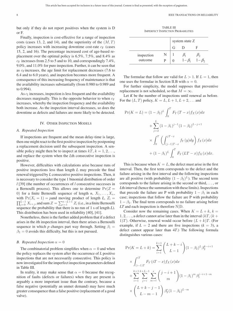
TABLE IIIIMPERFECT INSPECTION PROBABILITIES

The formulae that follow are valid for L > 1. If L = 1, thenone uses the formulae in Section II.B with α = 0.

For further simplicity, the model supposes that preventivereplacement is not scheduled, so that M = ∞.

Let K be the number of inspections until renewal as before.For the (L, T ) policy, K = L,L + 1, L + 2, . . . and

Pr(K = L) = (1 − β2)L

∫ T


+L∑

j=2

(1 − β1)j−1(1 − β2)

L−j+1

×∫ T

0

(∫ jT −x

(j−1)T −x

fY (y)dy

)fX (x)dx

+ (1 − β1)L

∫ T

0FY (LT − x)fX (x)dx.

This is because when K = L, the defect must arise in the firstinterval. Then, the first term corresponds to the defect and thefailure arising in the first interval and the following inspectionsare all positive (with probability (1 − β2)L ). The second termcorresponds to the failure arising in the second or third, . . . , orLth interval (hence the summation with these limits). Inspectionsthat precede the failure are P with probability 1 − β1 in eachcase; inspections that follow the failure are P with probability1 − β2 . The final term corresponds to no failure arising beforeLT and each inspection is therefore N|D.

Consider now the remaining cases. When K = L + k, k =1, 2, . . ., a defect cannot arise later than in the interval (kT, (k +1)T ). Otherwise, renewal would occur before (L + k)T . (Forexample, if L = 2 and there are five inspections (k = 3), adefect cannot appear later than 4T.) The following formuladistinguishes various cases:

Pr(K = L + k) =k+1∑i=1

(L + k − i

L − 1

)(1 − β2)Lβk−i+1

2

×∫ iT


+k+1∑i=1

k+L−1∑j=i

s∑m=t

(j − i + 1

m

)(1 − β1)

m βj−i+1−m1

×(

L + k − j − 1

L − m − 1

)βr

2 (1 − β2)L−m



×∫ iT

(i−1)T

∫ (j+1)T −x

jT −x

fY (y)dyfX (x)dx

+k+1∑i=1

(L + k − i

L − 1

)βk−i+1

1 (1 − β1)L

×∫ iT

(i−1)TFY ((L + k)T − x)fX (x)dx

with s = min{L − 1, j − i + 1}, t = max{0, j − k}, and r =max{0, k − j + m}.

The first summation in this expression corresponds to the casein which defect and failure occur in the same interval. If so, adefect cannot occur later than in (kT, (k + 1)T ). In the secondsummation, defect and failure occur in different intervals anda defect cannot occur later than in (kT, (k + 1)T ). The thirdsummation considers the case when a defect occurs but there isno failure.

The expected number of inspections is given by

E(K) = L +∞∑

k=1

k Pr(K = L + k)

which can be alternatively written as

E(K) = L +∞∑

k=1

Pr(K ≥ L + k).

The downtime calculation proceeds as follows. Let Ik be anindicator function for the event that a failed system is renewedat the (L + k)th inspection. Observe that Ik = 1 if and only ifIj = 0 j �= k. It therefore follows that the downtime is given by

W =∞∑

k=0

WL+k × Ik

where WL+k is the downtime incurred when the system is re-newed at the (L + k)th inspection.

For k = 0, it follows that

E(WL × I0)

= (1 − β2)L

∫ T

0

∫ T −x

0(LT − x − y)fY (y)dyfX (x)dx

+L∑

j=2

(1 − β1)j−1(1 − β2)

L−j+1

×∫ T

0

(∫ jT −x

(j−1)T −x

(LT − x − y)fY (y)dy

)fX (x)dx

and for k > 0

E(WL+k × Ik )

=k+1∑i=1

(L + k − i

L − 1

)(1 − β2)Lβk−i+1

2

×∫ iT

(i−1)T

∫ iT −x

0((L + k)T − x − y)fY (y)dyfX (x)dx

+k+1∑i=1

k+L−1∑j=i

s∑m=t

(j − i + 1

m

)(1 − β1)

m βj−i+1−m1

×(

L + k − j − 1

L − m − 1

)βr

2 (1 − β2)L−m

×∫ iT

(i−1)T

∫ (j+1)T −x

jT −x

((L + k)T − x − y)fY (y)fX (x)dy dx.

The expected downtime in a renewal cycle is then

E(W ) =∞∑

k=0

E(WL+k × Ik )

and the cost-rate is

Q(L, T ) = {cIE(K) + cFE(W ) + cR}/(T × E(K)).

The availability, or uptime, is given by

A(L, T ) = 1 − E(W )(T × E(K))

= 1 −∑∞

k=0 E(WL+k × Ik )∑∞k=0 T (L + k) Pr(K = L + k)

.

The repeated inspection policy may be justified when themaintainer wants to extend system lifetime. Thus, the maintaineris inclined to consider that a positive inspection is the result ofa system that is defective rather than failed.

Also, it may be interesting to determine the cost of a repeatedinspection policy in these circumstances in order to understandthe cost of “ignorance,” whereby a maintainer uses a policy(repeated inspection) that is necessarily cost-sub-optimal. Inpractice, one would wish to make a maintainer aware of thecost of procrastination. If a maintainer does not seek immediatereplacement, then postponement of replacement may be pre-ferred. This policy is considered in the next section. But, firstsome numerical results for the repeated inspection policy areconsidered briefly.

Again it is assumed that α = 0 and the parameter values as inSection III are used. Table IV briefly shows some results, and itcan be seen that in each case L∗ = 1 as expected. Regarding thecost of “ignorance,” the marginal increased cost of repeated in-spections can be calculated. Therein, repeated inspection leadsto greater cost and lower availability with increasing L. Themarginal increased cost of repeated inspection is greatest whenthe mean delay-time is the smallest (39% for L = 2 when λ = 2and 44% for L = 2 when λ = 0.5). Also, as L increases, T∗ de-creases (more frequent inspection) but not so much that LT∗ re-mains constant. Thus, increasing the inspection frequency doesnot compensate for repeated inspection, presumably becauseof the imperfect inspection. Indeed, for larger β1 or β2 , LT∗

increases with L more rapidly than for smaller β1 or β2 .

C. Postponed Replacement, α = 0

The inspection parameters are assumed as in Table III. Oncea positive inspection has occurred, at kT say, it is supposed thatthe maintainer decides to postpone replacement for a time τ ;



TABLE IVRESULTS FOR REPEATED INSPECTION POLICY

during this period of postponement (kT, kT + τ), there are nofurther inspections. The rationale is that the maintainer seeks toextend the system life with a minimal cost, taking advantage ofthe delay-time, the time for which the system is defective butfunctional. Furthermore, the maintainer is aware that a prob-lem exists and new inspections would incur an extra cost for asystem that is close to replacement. Note, the cost-rate can bedeveloped for α > 0, but since this policy follows naturally fromthe previous (repeated inspection), the supposition that α = 0 iscontinued.

Another aspect already mentioned is that an N|D or N|Finspection may be of greater concern that a P|G inspection.

Let K be the number of inspections until renewal, K =1, 2, . . . In this model, K is the number of inspections upto including the first positive inspection, and it follows thatPr(K = 1), Pr(K = 2), and Pr(K = k) are given by (1), (2),and (4), respectively, but with α = 0. Thus, K has the same dis-tribution as the policy in Section II.B (policy 1) with M = ∞.Furthermore, when τ = 0, policy 1 is obtained as a special casewith α = 0.

The cycle length for this postponed replacement policy has themodification for the additional period of postponement. Thus,the expected cycle length is

E(Vτ ) = τ +∞∑

k=1

kT Pr(K = k).

The downtime is different to policy 1, but in principle, thederivation is similar. Thus, consider the event Sk : inspection atkT is positive and the defect arises at time x and the failurey time units later. The downtime conditional on Sk is Δxy =kT + τ − x − y, and the expected downtime is (for τ > 0)

E(Wτ ) =∞∑

i=1

(1 − β2)

×{ ∞∑

k=i

βk−i2

∫ iT

(i−1)T

{∫ iT −x

0Δxy fY (y)dy

}fX (x)dx

+∞∑

j=i

∞∑k=j+1

βj−i+11 βk−j−1

2

×∫ iT

(i−1)T

{∫ (j+1)T −x

jT −x

Δxy fY (y)dy

}fX (x)dx

}

+∞∑

i=1

∞∑k=i

(1 − β1)βk−i1

×∫ iT

(i−1)T

{∫ kT +τ−x

kT −x

Δxy fY (y)dy

}fX (x)dx.

Here, in the first term, the defect and failure occur in the sameinterval ((i − 1)T, iT ) and the failure is detected at kT, k > i. Inthe second term the failure occurs in the interval ((j − 1)T, jT )subsequent to that of the defect and the failure is detected atkT, k > j + 1. In both cases, the positive inspection is due toa failure, so it is a true positive. In the final term, a defect isdetected at kT and the failure occurs during the interval ofpostponement (kT, kT + τ).

The expected cost of a cycle is then

E(Uτ ) = cI

∞∑k=1

k Pr(K = k) + cFE(Wτ ) + cR .

For the parameter values in the cases in Table II, it followsthat τ ∗ = 0 always, and so for brevity, these results are omit-ted. The optimality of τ ∗ = 0 is contrary to the examples in[31] wherein α �= 0 and the possibility of opportunity-basedmaintenance means τ ∗ > 0 is optimum.

Nonetheless, it is interesting to consider the cost-rate if themaintainer acts sub-optimally and postpones replacement. In-deed, Fig. 6 indicates that postponement is not a good policy,because of the possibility that the system is failed at a positiveinspection and the consequent downtime is costly. Moreover,postponement is less appropriate when β2 is larger.

However, when β2 = 0, the cost rises more rapidly than forβ2 > 0, which is curious. This is perhaps because T is held at itsoptimum value for τ = 0, and τ > 0 may imply a smaller T∗.Nonetheless, for β2 = 0 and a large mean delay-time, it mightbe expected that postponement is optimal.



Fig. 6. Cost-rate Q as a function of the length of postponement τ for β2 = 0(dash line), β2 = 0.1 (dotted), β2 = 0.2 (solid), and with T at its optimal valuefor the respective β2 and other parameters as base case (see case 2 in Table II).

Finally, a policy in which the first positive inspection triggersa deeper, more costly inspection that verifies the state of thesystem can be considered. Then, postponement only occurs if thesystem is defective (noting that because α = 0 the system cannotbe G). However, consideration of such a two stage inspectionpolicy is beyond the scope of this paper.

Other related analyses are also possible. For example, if twoinspection tests were available, with costs cI1 and cI2 suchthat the cheaper inspection was less effective, then one couldask which test is preferred. Alternatively, one might considerwhat is an appropriate investment to improve inspection testeffectiveness.

V. CONCLUSION

This paper studied imperfect inspection of a protection sys-tem. This system is subject to a three-state (G, D, and F) failureprocess, and sojourns in the G and D states are random vari-ables. The inspection outcome provides imperfect informationabout the system state that is quantified through a set of proba-bilities that are parameterized in the model. Given then a levelof ignorance about the state of the protection system followingan inspection, the maintainer must decide whether to replace thesystem. At a higher level, the maintainer must decide whether toinspect. These decisions are studied by developing the cost-rateof an inspection and replacement policy that is natural in thiscontext.

The novelty of the paper is the consideration of imperfectinspection for a protection system subject to a state (defective)that lies between the good and the failed states. Imperfect in-spections can occur in both states although is less likely whenthe system is failed than defective. This mimicks inspection ofsystems in real life. Thus, the benefit of modeling the defec-tive state is that this may better represent the reality in whichinspection provides imperfect information about the true un-derlying state of the protection system. Given this uncertainty,the maintainer must decide if inspection is an effective strategy.Further, interest in modeling the defective state also emerges ifthe duration of use on-demand is nonnegligible, so that thereis the possibility of failure during the demand period when thesystem is defective at the start of the demand period. However,this would be another study.

The analysis in this paper shows first that, since inspectionmight not be effective, it is natural that a maintainer would inignorance replace the system at a particular age. The cases ana-lyzed in the numerical example show that this policy is effectivenot only in terms of cost but also concerning availability. Thus,preventive maintenance at MT is protection against low-qualityinspections. Then, second, the analysis shows that inspectionis cost-effective provided the imperfect inspection probabilitiesare not too large. Therein, the most important (to the cost-rate)is α = Pr(P|G). Finally, it was shown that there exist circum-stances in which a pure inspection policy is near-cost-optimal.However, even when inspection is perfect, ageing of the systemimplies that preventive replacement at MT remains a sensiblepolicy. A two-stage policy that is an adaptation to the increas-ing hazard-rate of an ageing system may provide further cost-benefit. This would be another study.

The inclusion in the model of an additional imperfect in-spection probability β2 adds another level of complexity to thecost-rate function. Thus, the expressions for the cost-rate aswell as its derivative are rather complicated. This leads to anempirical study with no analytical results. Nevertheless, sinceinspection aims to detect defective and failed states, only smalland medium values of T constitute the region of interest. Theresults in Tables II and IV present the global optimum in thatregion at least.

For the repeated inspection policy, the imperfect inspectionprobabilities are simplified in order to calculate the cost-rateand availability. Then, it is found that repeated inspection leadsto high cost and downtime, and postponement of replacementis not a good decision. However, this sub-optimality is in partdue to the simplification (because it is likely that postponementwould be justified when α > 0). Corresponding calculations inthe general case (with a full set of imperfect inspection proba-bilities) would make an interesting and challenging study andmay determine circumstances in which repeated inspection ispreferable.

It would be interesting to consider imperfection in inspectionwhen inspection reports the system state (G, D, or F) rather thanthe functionality of the system (N or P). This is a new, differentmodel worthy of future investigation.

ACKNOWLEDGMENT

The authors would like to thank the anonymous reviewers fortheir valuable comments.

REFERENCES

[1] S. Lavery and B. Donovan, “Flood risk management in the thames estuarylooking ahead 100 years,” Philos. Trans. Roy. Soc. A, vol. 363, pp. 1455–1474, 2005.

[2] L. Wang, H. Hu, Y. Wang, W. Wu, and P. He, “The availability model andparameters estimation method for the delay-time model with imperfectmaintenance at inspection,” Appl. Math. Model., vol. 35, pp. 2855–2863,2011.

[3] R. Flage, “A delay-time model with imperfect and failure-inducing in-spections,” Rel. Eng. Syst. Safety, vol. 124, pp. 1–12, 2014.

[4] J. P. C. Driessen, H. Peng, and G. J. van Houtum, “Maintenance optimiza-tion under nonconstant probabilities of imperfect inspections,” Rel. Eng.Syst. Safety, vol. 165, pp. 115–123, 2017.



[5] M. D. Berrade, P. A. Scarf, and C. A. V. Cavalcante, “Maintenancescheduling of a protection system subject to imperfect inspection andreplacement,” Eur. J. Oper. Res., vol. 218, pp. 716–725, 2012.

[6] M. D. Berrade, P. A. Scarf, and C. A. V. Cavalcante, “Some insights intothe effect of maintenance quality for a protection system,” IEEE Trans.Rel., vol. 64, no. 2, pp. 661–672, Jun. 2015.

[7] X. Jia and A. H. Christer, “A periodic testing model for a preparednesssystem with a defective state,” IMA J. Manag. Math., vol. 13, pp. 39–49,2002.

[8] C. A. V. Cavalcante, P. A. Scarf, and A. de Almeida, “A study of a two-phase inspection policy for a preparedness system with a defective stateand heterogeneous lifetime,” Rel. Eng. Syst. Safety, vol. 69, pp. 627–635,2011.

[9] A. H. Christer, “Delay-time model of reliability of equipment subject toinspection monitoring,” J. Oper. Res. Soc., vol. 38, no. 4, pp. 329–334,1987.

[10] A. R. Alberti, C. A. V. Cavalcante, A. L. O. Silva, and P. A. Scarf,“Modelling inspection and replacement quality for a protection system,”Rel. Eng. Syst. Safety, vol. 176, pp. 145–153, 2018.

[11] Y. Dai, G. Levitin, and L. Xing, “Optimal periodic inspections and acti-vation sequencing policy in standby systems with condition-based modetransfer,” IEEE Trans. Rel., vol. 66, no. 1, pp. 189–201, Mar. 2017.

[12] P. A. Scarf, C. A. V. Cavalcante, R. A. Dwight, and P. Gordon, “An age-based inspection and replacement policy for heterogeneous components,”IEEE Trans. Rel., vol. 58, no. 4, pp. 641–648, Dec. 2009.

[13] C. D. Van Oosterom, A. H. Elwany, D. Celebi, and G. J. Van Houtum,“Optimal policies for a delay time model with postponed replacement,”Eur. J. Oper. Res., vol. 232, pp. 186–197, 2014.

[14] L. Yang, X. Ma, Q. Zhai, and Y. Zhao, “A delay time model for a mission-based system subject to periodic and random inspection and postponedreplacement,” Rel. Eng. Syst. Safety, vol. 150, pp. 96–104, 2016.

[15] M. Mahmoudi, A. Elwany, K. Shahanaghi, and M. R. Gholamian, “A delaytime model with multiple defect types and multiple inspection methods,”IEEE Trans. Rel., vol. 66, no. 4, pp. 1073–1084, Dec. 2017.

[16] S. Taghipour and S. Azimpoor, “Joint optimization of jobs sequence andinspection policy for a single system with two-stage failure process,” IEEETrans. Rel., vol. 67, no. 1, pp. 156–169, Mar. 2018.

[17] L. Yang, Z. S. Ye, C. G. Lee, S. F. Yang, and R. Peng, “A two-phasepreventive maintenance policy considering imperfect repair and postponedreplacement,” Eur. J. Oper. Res., vol. 274, pp. 966–977, 2019.

[18] W. Wang, “An inspection model based on a three-stage failure process,”Rel. Eng. Syst. Safety, vol. 96, pp. 838–848, 2011.

[19] W. Wang, F. Zhao, and R. Peng, “A preventive maintenance model witha two-level inspection policy based on a three-stage failure process,” Rel.Eng. Syst. Safety, vol. 121, pp. 207–220, 2014.

[20] H. Wang, W. Wang, and R. Peng, “A two-phase inspection model for asingle component system with three stage degradation,” Rel. Eng. Syst.Safety, vol. 158, pp. 31–40, 2017.

[21] M. S. Pepe, The Statistical Evaluation of Medical Tests for Classificationand Prediction. Oxford, U.K.: Oxford Univ. Press; 2003.

[22] P. A. Scarf, “On the application of mathematical models in maintenance,”Eur. J. Oper. Res., vol. 99, pp. 493–506, 1997.

[23] P. A. Scarf and C. A. V. Cavalcante, “Modeling quality in replacementand inspection maintenance,” Int. J. Prod. Econ., vol. 135, pp. 373–391,2012.

[24] B. S. Dhillon and Y. Liu, “Human error in maintenance: A review,” J.Qual. Maintenance Eng., vol. 12, no. 1, pp. 21–36, 2006.

[25] A. Noroozi, F. Khan, S. MacKinnon, P. Amyotte, and T. Deacon, “De-termination of human error probabilities in maintenance procedures of apump,” Process Safety Environ. Protection, vol. 92, no. 2, pp. 131–141,2014.

[26] H. Ascher and F. Feingold, Repairable Systems Reliability. New York,NY, USA: Marcel Dekker, 1984.

[27] W. Wang, “An overview of the recent advances in delay-time-based main-tenance modeling,” Rel. Eng. Syst. Safety, vol. 106, pp. 165–178, 2012.

[28] J. K. Vaurio, “Unavailability analysis of periodically tested standby com-ponents,” IEEE Trans. Rel., vol. 44, no. 3, pp. 512–517, Sep. 1995.

[29] J. K. Vaurio, “Availability and cost functions for periodically inspectedpreventively maintained units,” Rel. Eng. Syst. Safety, vol. 63, pp. 133–140, 1999.

[30] M. D. Berrade, P. A. Scarf, C. A. V. Cavalcante, and R. A. Dwight,“Imperfect inspection and replacement of a system with a defective state:A cost and reliability analysis,” Rel. Eng. Syst. Safety, vol. 120, pp. 80–87,2013.

[31] M. D. Berrade, P. A. Scarf, and C. A. V. Cavalcante, “A study of postponedreplacement in a delay-time model,” Rel. Eng. Syst. Safety, vol. 168,pp. 70–79, 2017.

[32] F. G. Badıa, M. D. Berrade, and C. A. Campos, “Optimization of inspectionintervals based on cost,” J. Appl. Probability, vol. 38, pp. 872–881, 2001.

[33] F. G. Badıa, M. D. Berrade, and C. A. Campos, “Optimal inspection andpreventive maintenance of units with revealed and unrevealed failures,”Rel. Eng. Syst. Safety, vol. 78, pp. 157–163, 2002.

[34] M. D. Berrade, C. A. V. Cavalcante,and P. A. Scarf, “Modeling imperfectinspection over a finite horizon,” Rel. Eng. Syst. Safety, vol. 111, pp. 18–29,2013.

[35] S. Y. Sohn, “Accelerated life-tests for intermittent destructive inspection,with logistic failure-distribution,” IEEE Trans. Rel., vol. 46, no. 1, pp. 122–129, Mar. 1997.

[36] A. Labib and M. J. Harris, “Learning how to learn from failures: TheFukushima nuclear disaster,” Eng. Failure Anal., vol. 47, pp. 117–128,2015.

[37] S. Ross, Stochastic Processes. New York, NY, USA: Wiley, 1996.[38] M. D. Berrade, “A two-phase inspection policy with imperfect testing,”

Appl. Math. Model., vol. 36, pp. 108–114, 2012.[39] N. L. Johnson, A. W. Kemp, and S. Kotz, Univariate Discrete Distribu-

tions. New York, NY, USA: Wiley, 2005.[40] J. G. Shanthikumar, “Recursive algorithm to evaluate the reliability of

a consecutive k-out-of- n:F system,” IEEE Trans. Rel., vol. 31, no. 5,pp. 442–443, Dec. 1982.

[41] K. D. Ling, “On binomial distributions of order k,” Statist. ProbabilityLett., vol. 6, pp. 247–250, 1988.

Cristiano A. V. Cavalcante (M’10) received thePh.D. degree in operational research from Universi-dade Federal de Pernambuco, Recife, Brazil, in 2005.

He is a Senior Lecturer of operational research,maintenance engineering and logistics at the Fed-eral University of Pernambuco, Brazil. He has au-thored or coauthored more than 30 scientific papersin peer-reviewed journals on topics related to: oper-ational research, maintenance modeling, risk, relia-bility, safety, warehouse management, warranty, andMCDM/A (multicriteria decision making and aid).

Dr. Cavalcante has been the recipient of a research fellowship from theBrazil National Research Council (CNPq) since 2009. Also, he is the leaderof RANDOM (Research Group on Risk and Decision Analysis in Operationsand Maintenance) at UFPE and is an Associate Member of CDSID (Center forDecision Systems and Information Development). He is a Fellow of the Instituteof Mathematics and Its Applications (IMA, U.K.) and a Member of the Institutefor Operations Research and Management Science (INFORMS).

Philip Scarf received the Ph.D. degree in statis-tics from the University of Manchester, Manchester,U.K., in 1989.

He is a Professor of Applied Statistics at the Uni-versity of Salford, U.K. He has authored or coau-thored more than 40 articles on the modeling ofcapital replacement, reliability, and maintenance inleading peer-reviewed journals. His research inter-ests include advanced robotics, extreme values, crackgrowth, and applications of operational research andstatistics in sports.

Dr. Scarf is the Chair of the IMA Conference on Modelling in Maintenanceand Reliability; the 11th conference in the series will take place in 2020. He isa Fellow of the Royal Statistical Society (U.K.) and a Fellow of the Institute ofMathematics and Its Applications (IMA, U.K.). He serves as Editor-in-Chief ofthe IMA Journal of Management Mathematics.

M. D. Berrade received the Ph.D. degree in math-ematics from the University of Zaragoza, Zaragoza,Spain, in 1999.

She is a tenured Professor of Statistics at the Uni-versity of Zaragoza, Spain. Her work is publishedin IEEE TRANSACTIONS ON RELIABILITY, ReliabilityEngineering and System Safety, Applied Mathemati-cal Modelling, European Journal of Operational Re-search, the Journal of Applied Probability, AppliedStochastic Models in Business and Industry, Prob-ability in the Engineering and Informational Sci-

ences, and others. Her research interests include inspection and maintenanceof systems.

Documents

Imperfect Inspection of a System With Unrevealed Failure