Implementation of a Raman Sideband Coolingfor 87Rb

Bachelorarbeit vonChristoph Braun

05.10.2015

Universitat Stuttgart5. Physikalisches Institut

Prof. Dr. Tilman PfauDr. Sebastian Hofferberth

Implementierung einer Raman Seitenband Huhlung fur 87Rb

Zusammenfassung Im Rahmen dieser Arbeit wurde ein Aufbau realisiert um Atomeselbst bei hohen Dichten weiter effizient kuhlen zu konnen. Das entartete Raman Seiten-band Kuhlen ermoglicht hohere Dichten und niedrigere Temperaturen als die Kuhlungmittels magneto-optischer Falle sowie folgender optischer Molasse und Kompression. Daruberhinaus bestunde die Moglichkeit Atome innerhalb einer optischen Dipolfalle zu kuhlenjedoch wird beim Raman Seitenband Kuhlen gegenuber dem Verdampfungskuhlen dieAtomzahl weniger reduziert.

In der vorliegenden Arbeit wird zunachst die grundlegende Struktur der atomaren Ener-gieniveaus erlautert, daraufhin werden die grundlegenden Elemente des Aufbaus beschrie-ben sowie die Intensitatsstabilisierung naher charakterisiert. Der grundsatzliche Ablaufeines Kuhlzyklus auf atomarer Ebene wird erklart und spater die Kopplung zwischen denmagnetischen Hyperfeinstrtukturniveaus diskutiert. Die erwartbare Leistungsfahigkeit desgesamten Prozesses wird gemeinsam mit den ersten Messungen im Zusammenhang mitdieser Kuhlmethode vorgestellt.

Implementation of a Raman Sideband Cooling for 87Rb

Abstract In the Course of this thesis a setup which theoretically enables efficient coolingeven at high densities has been realized. Degenerate Raman sideband cooling makes itpossible to cool to lower temperatures and higher densities than achievable with commonmagneto-optical trapping and subsequent optical molasses and compression. Furthermorethis cooling process could be implemented inside an optical dipole trap where cooling withless loss of trapped atoms could be achieved in comparison to evaporative cooling.

In the presented thesis the basic structure of atomic energy levels is illustrated, nextthe basic elements of the setup are described and the characteristics of the intensitystabilization are specified. The process of cooling is explained on the single atom leveltogether with the origin of the coupling between different magnetic hyperfine levels. Theexpectable performance is discussed along with the first measurements conducted in con-nection with Raman sideband cooling.

3

Declaration

I hereby declare that this submission is my own work and that, to the best of my knowledge andbelief, it contains no material previously published or written by another person, except where dueacknowledgment has been made in the text.

Christoph BraunStuttgart, October 5, 2015

4

Contents

1. The Rubidium Atom 61.1. Atomic Structure . . . . . . . . . . . . . . . . . . . . . . . . . . . . . . . . . . . . . . . 61.2. Fine-structure . . . . . . . . . . . . . . . . . . . . . . . . . . . . . . . . . . . . . . . . . 61.3. Hyperfine-structure . . . . . . . . . . . . . . . . . . . . . . . . . . . . . . . . . . . . . . 71.4. Zeeman Effect . . . . . . . . . . . . . . . . . . . . . . . . . . . . . . . . . . . . . . . . . 7

2. Setup 72.1. Lattice Laser . . . . . . . . . . . . . . . . . . . . . . . . . . . . . . . . . . . . . . . . . 72.2. Raman-Pump Laser . . . . . . . . . . . . . . . . . . . . . . . . . . . . . . . . . . . . . 102.3. Lattice Optics and Intensity Stabilization . . . . . . . . . . . . . . . . . . . . . . . . . 10

2.3.1. Intensity Stabilization Electronics . . . . . . . . . . . . . . . . . . . . . . . . . 102.3.2. Intensity Stabilization and Lattice Optics . . . . . . . . . . . . . . . . . . . . . 13

2.4. Additional Elements used in this Experiment . . . . . . . . . . . . . . . . . . . . . . . 14

3. Explanation of a Cooling Cycle 143.1. Origin of Sidebands . . . . . . . . . . . . . . . . . . . . . . . . . . . . . . . . . . . . . 143.2. The Cooling Process . . . . . . . . . . . . . . . . . . . . . . . . . . . . . . . . . . . . . 15

4. Calculation of the Lattice Potential 174.1. Derivation of the Light-Induced Potential for a 2-Level System . . . . . . . . . . . . . 174.2. Resulting Lattice and Approximation . . . . . . . . . . . . . . . . . . . . . . . . . . . . 19

4.2.1. The Polarizability Tensor . . . . . . . . . . . . . . . . . . . . . . . . . . . . . . 194.2.2. Calculation of the Lattice Characteristics . . . . . . . . . . . . . . . . . . . . . 214.2.3. Motivating the Harmonic Oscillator Approximation . . . . . . . . . . . . . . . 264.2.4. Raman Coupling . . . . . . . . . . . . . . . . . . . . . . . . . . . . . . . . . . . 274.2.5. Linewidth of the Raman transitions . . . . . . . . . . . . . . . . . . . . . . . . 28

4.3. Scattering Rate and Estimated Cooling Rate . . . . . . . . . . . . . . . . . . . . . . . 28

5. Conducted Measurements 295.1. Magnetic Field Nullification . . . . . . . . . . . . . . . . . . . . . . . . . . . . . . . . . 305.2. Polarization Stability . . . . . . . . . . . . . . . . . . . . . . . . . . . . . . . . . . . . . 315.3. Aligning the Raman Lattice Beams . . . . . . . . . . . . . . . . . . . . . . . . . . . . . 325.4. Adiabatic Release and Capture . . . . . . . . . . . . . . . . . . . . . . . . . . . . . . . 325.5. Testing the Raman Sideband Cooling . . . . . . . . . . . . . . . . . . . . . . . . . . . . 34

6. Conclusion and Outlook 37

A. PID 39

B. Matrices of the Polarizability Tensor 40

C. References 41

5

1. The Rubidium Atom

1.1. Atomic Structure

The Rubidium Atom is one of the alkali metals. The alkali atoms lying in the first group of theperiodic table all have in common that their outermost electron is in an s-orbital. The beneficialthing about that is that the inner electrons in the closed shells do not contribute to the total spinand angular momentum, therefore the quantum mechanical description of the hydrogen atom canbe adapted. As there is obviously more than one electron one has to consider the electron-electronand electron-nucleus interaction in the Hamiltonian. A simple approach just assumes that the innerelectrons sort of shield the nucleus’ core resulting in a single charged core and an electron. The resultwould be the binding energies of the hydrogen atom, as this is not true one can modify the principalquantum number n depending on the outer electron’s orbital. This correction is known as quantumdefect [Foot, 2005]. With the assumptions discussed one can calculate the spin-orbit interaction andthe ongoing hyperfine structure arising from the nuclear spin interacting with the electron spin andorbit.

1.2. Fine-structure

In 1922 Stern and Gerlach discovered the electron spin due to its interaction with magnetic fields[Gerlach and Stern, 1922]. An electron orbiting a nucleus could in principle also be considered asa current resulting in a magnetic field with which the electron spin could interact. Following thisconsideration the angular momentum - embodying the orbital movement - should give rise to anenergy difference in the atomic energy structure. As the angular momentum of an electron doescontribute to the energy levels of the atom, the arising energy difference is called fine-structuresplitting. The Hamiltonian results from the Lorentz transformation for electromagnetic fields or ina more complex from the Dirac equation. In a ”classical” approach the electron sees the electricfield of the core resulting in a magnetic field which is coupling to the electron’s spin, resulting in thefollowing Hamiltonian in spherical coordinates,

HFS = − ~µs · ~B =µBgs∂rV (r)

mc2~er~L · ~S. (1)

Here µB is the Bohr magneton, gs the electron spin g-factor, m the electron’s rest mass, c the speedof light and e the elementary charge. Due to the transformation back to the laboratory frame arisesa term, the so called Thomas precession [Jackson, 1982]

HT = −µB∂rV (r)

mc2~er~L · ~S. (2)

The single angular momentum operators ~L and ~S are now coupled and result in new quantum num-

bers ~J and mJ , the composed angular momentum. Note that the basis of ~L and ~S does not lose itsvalidity but the projection of the angular momentum operator, e.g. Lz (quantization axis along z),is no longer diagonal in this basis, therefore it’s convenient to change the basis and introduce newoperators. Consequently the total energy shift caused by the spin-orbit interaction is

∆EFS 〈n,L,S,J,mJ |HFS +HT |n,L,S,J,mJ〉 =

µB(gs − 1) 〈n|∂rV (r)|n〉mc2~er

[J(J + 1)− L(L+ 1)− S(S + 1)].(3)

6

1.3. Hyperfine-structure

The nuclear spin’s ~I magnetic moment is given by

~µI = gIµN ~I, (4)

it interacts in a similar way with a magnetic field arising from the interaction of the core with theelectron’s spin and orbit. The derivation follows analogous, with some more terms. The resulting

angular momentum ~I and therefore also mF is composed from ~J and ~I. The energy shift [Steck,2001], if only the magnetic dipole moment is taken into account, reads

∆EHFS =1

2AHFS[F (F + 1)− I(I + 1)− J(J + 1)], (5)

where AHFS is called hyperfine-structure constant, which also depends on the atoms state. To givea rough example for 87Rb in 52S1/2 the hyperfine-structure constant is AHFS = h · 3.417 GHz [Steck,2001].

1.4. Zeeman Effect

As described above, the atom’s electron(s) interact with electromagnetic fields. If a magnetic field isapplied the Hamilton-operator is composed by

HB =µB~

(gs ~S + gI ~I + gL ~L) ·B. (6)

In general the resulting Hamiltonian HHFS +HB needs to be calculated and diagonalized to find theresulting energy shift, often one does not find an analytical solution so the calculation needs to bedone numerically. For a state with J = 1/2, e.g. the Rb groundstate, the Breit-Rabi formula can beobtained, the direction of the magnetic field defines the quantization axis then, preferably z.

∆E|J=1/2,mJ ,mI〉 = −AHFS(I + 1/2)

2(2I + 1)+ µBgI

(mI +

1

2

)B

± AHFS(I + 1/2)

2

[1 + 2

µB(gJ − gI)BAHFS(I + 1/2)

2mI + 1

2I + 1+

(µB(gJ − gI)BAHFS(I + 1/2)

)2]1/2 (7)

gJ = 1 +J(J + 1)− L(L+ 1) + S(S + 1)

2J(J + 1)(8)

gI,87Rb = −0.000995 (9)

(10)

2. Setup

2.1. Lattice Laser

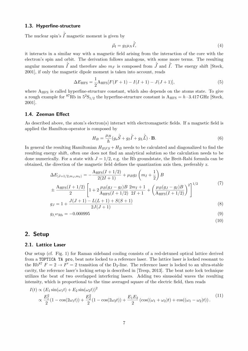
Our setup (cf. Fig. 1) for Raman sideband cooling consists of a red-detuned optical lattice derivedfrom a TOPTICA TA pro, beat note locked to a reference laser. The lattice laser is locked resonant tothe Rb87 F = 2 → F ′ = 2 transition of the D2-line. The reference laser is locked to an ultra-stablecavity, the reference laser’s locking setup is described in [Tresp, 2013]. The beat note lock techniqueutilizes the beat of two overlapped interfering lasers. Adding two sinusoidal waves the resultingintensity, which is proportional to the time averaged square of the electric field, then reads

I(t) ∝ (E1 sin(ω1t) + E2 sin(ω2t))2

∝ E21

2(1− cos(2ω1t)) +

E22

2(1− cos(2ω2t)) +

E1E2

2(cos((ω1 + ω2)t) + cos((ω1 − ω2)t)) .

(11)

7

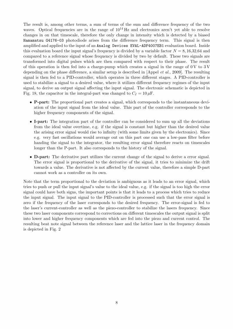
The result is, among other terms, a sum of terms of the sum and difference frequency of the twowaves. Optical frequencies are in the range of 1014 Hz and electronics aren’t yet able to resolvechanges in on that timescale, therefore the only change in intensity which is detected by a biasedHamamatsu G4176-03 photodiode arises from the difference frequency term. This signal is thenamplified and applied to the input of an Analog Devices EVAL-ADF4007EB1 evaluation board. Insidethis evaluation board the input signal’s frequency is divided by a variable factor N = 8, 16,32,64 andcompared to a reference signal whose frequency is divided by two by default. These two signals aretransformed into digital pulses which are then compared with respect to their phase. The resultof this operation is then fed into a charge-pump which creates a signal in the range of 0 V to 3 Vdepending on the phase difference, a similar setup is described in [Appel et al., 2009]. The resultingsignal is then fed to a PID-controller, which operates in three different stages. A PID-controller isused to stabilize a signal to a desired value, where it utilizes different frequency regimes of the inputsignal, to derive an output signal affecting the input signal. The electronic schematic is depicted inFig. 18, the capacitor in the integral-part was changed to CI = 10µF.

• P-part: The proportional part creates a signal, which corresponds to the instantaneous devi-ation of the input signal from the ideal value. This part of the controller corresponds to thehigher frequency components of the signal.

• I-part: The integration part of the controller can be considered to sum up all the deviationsfrom the ideal value overtime, e.g. if the signal is constant but higher than the desired valuethe arising error signal would rise to infinity (with some limits given by the electronics). Sincee.g. very fast oscillations would average out on this part one can use a low-pass filter beforehanding the signal to the integrator, the resulting error signal therefore reacts on timescaleslonger than the P-part. It also corresponds to the history of the signal.

• D-part: The derivative part utilizes the current change of the signal to derive a error signal.The error signal is proportional to the derivative of the signal, it tries to minimize the drifttowards a value. The derivative is not affected by the current value, therefore a simple D-partcannot work as a controller on its own.

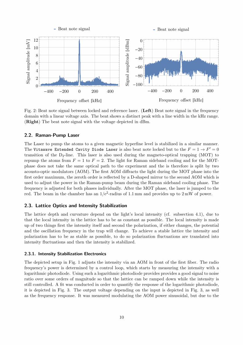
Note that the term proportional to the deviation is ambiguous as it leads to an error signal, whichtries to push or pull the input signal’s value to the ideal value, e.g. if the signal is too high the errorsignal could have both signs, the important points is that it leads to a process which tries to reducethe input signal. The input signal to the PID-controller is processed such that the error signal iszero if the frequency of the laser corresponds to the desired frequency. The error-signal is fed tothe laser’s current-controller as well as the piezo-controller to stabilize the lasers frequency. Sincethese two laser components correspond to corrections on different timescales the output signal is splitinto lower and higher frequency components which are fed into the piezo and current control. Theresulting beat note signal between the reference laser and the lattice laser in the frequency domainis depicted in Fig. 2

8

Laser

λ/2

PBS

f=110mm shutter f=30mm AOM

Iris

λ/2

Fibercoupler

f=4.51mm

Fibercoupler

f=11mm

λ/2

PBS

λ/2PBSλ/2PBS

λ/2

50:50

PBS

PD

λ/2λ/2

λ/2

x

y

z

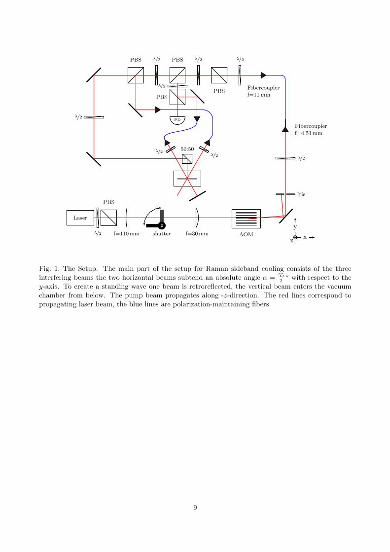
Fig. 1: The Setup. The main part of the setup for Raman sideband cooling consists of the threeinterfering beams the two horizontal beams subtend an absolute angle α = 55

2 with respect to the

y-axis. To create a standing wave one beam is retroreflected, the vertical beam enters the vacuumchamber from below. The pump beam propagates along -z-direction. The red lines correspond topropagating laser beam, the blue lines are polarization-maintaining fibers.

9

Beat note signal

-400 -200 0 200 40002468

1012

Frequency offset [kHz]

Sign

alam

plitu

de[m

V]

Beat note signal

-400 -200 0 200 400-100

-80

-60

-40

-20

0

Frequency offset [kHz]

Sign

alam

plitu

de[d

Bm]

Fig. 2: Beat note signal between locked and reference laser. (Left) Beat note signal in the frequencydomain with a linear voltage axis. The beat shows a distinct peak with a line width in the kHz range.(Right) The beat note signal with the voltage depicted in dBm.

2.2. Raman-Pump Laser

The Laser to pump the atoms to a given magnetic hyperfine level is stabilized in a similar manner.The Vitawave Extended Cavity Diode Laser is also beat note locked but to the F = 1→ F ′ = 0transition of the D2-line. This laser is also used during the magneto-optical trapping (MOT) torepump the atoms from F = 1 to F = 2. The light for Raman sideband cooling and for the MOT-phase does not take the same optical path to the experiment and the is therefore is split by twoacousto-optic modulators (AOM). The first AOM diffracts the light during the MOT phase into thefirst order maximum, the zeroth order is reflected by a D-shaped mirror to the second AOM which isused to adjust the power in the Raman-pump beam during the Raman sideband cooling phase. Thefrequency is adjusted for both phases individually. After the MOT phase, the laser is jumped to thered. The beam in the chamber has an 1/e2-radius of 1.1 mm and provides up to 2 mW of power.

2.3. Lattice Optics and Intensity Stabilization

The lattice depth and curvature depend on the light’s local intensity (cf. subsection 4.1), due tothat the local intensity in the lattice has to be as constant as possible. The local intensity is madeup of two things first the intensity itself and second the polarization, if either changes, the potentialand the oscillation frequency in the trap will change. To achieve a stable lattice the intensity andpolarization has to be as stable as possible, to do so polarization fluctuations are translated intointensity fluctuations and then the intensity is stabilized.

2.3.1. Intensity Stabilization Electronics

The depicted setup in Fig. 1 adjusts the intensity via an AOM in front of the first fiber. The radiofrequency’s power is determined by a control loop, which starts by measuring the intensity with alogarithmic photodiode. Using such a logarithmic photodiode provides provides a good signal to noiseratio over some orders of magnitude so that the lattice can be ramped down while the intensity isstill controlled. A fit was conducted in order to quantify the response of the logarithmic photodiode,it is depicted in Fig. 3. The output voltage depending on the input is depicted in Fig. 3, as wellas the frequency response. It was measured modulating the AOM power sinusoidal, but due to the

10

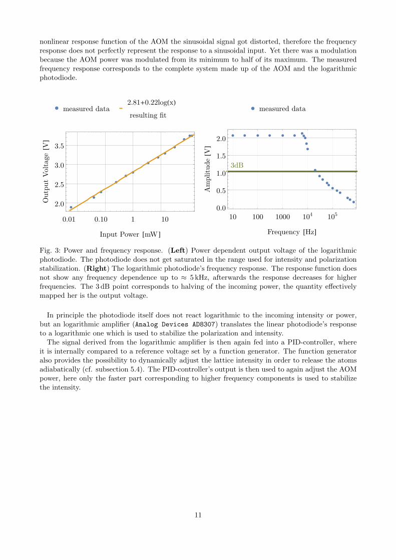
nonlinear response function of the AOM the sinusoidal signal got distorted, therefore the frequencyresponse does not perfectly represent the response to a sinusoidal input. Yet there was a modulationbecause the AOM power was modulated from its minimum to half of its maximum. The measuredfrequency response corresponds to the complete system made up of the AOM and the logarithmicphotodiode.

measured data2.81+0.22log(x)resulting fit

0.01 0.10 1 10

2.0

2.5

3.0

3.5

Input Power [mW]

Out

put

Volta

ge[V

]

measured data

3dB

10 100 1000 104 1050.0

0.5

1.0

1.5

2.0

Frequency [Hz]

Am

plitu

de[V

]

Fig. 3: Power and frequency response. (Left) Power dependent output voltage of the logarithmicphotodiode. The photodiode does not get saturated in the range used for intensity and polarizationstabilization. (Right) The logarithmic photodiode’s frequency response. The response function doesnot show any frequency dependence up to ≈ 5 kHz, afterwards the response decreases for higherfrequencies. The 3 dB point corresponds to halving of the incoming power, the quantity effectivelymapped her is the output voltage.

In principle the photodiode itself does not react logarithmic to the incoming intensity or power,but an logarithmic amplifier (Analog Devices AD8307) translates the linear photodiode’s responseto a logarithmic one which is used to stabilize the polarization and intensity.

The signal derived from the logarithmic amplifier is then again fed into a PID-controller, whereit is internally compared to a reference voltage set by a function generator. The function generatoralso provides the possibility to dynamically adjust the lattice intensity in order to release the atomsadiabatically (cf. subsection 5.4). The PID-controller’s output is then used to again adjust the AOMpower, here only the faster part corresponding to higher frequency components is used to stabilizethe intensity.

11

P-part I-part P+I-part

10 100 1000 104 105 106

0.050.10

0.501

510

Frequency [Hz]

Vpp

[V]

P-part I-part P+I-part

10 100 1000 104 105 106

180200220240260280300

Frequency [Hz]

Phas

e[°]

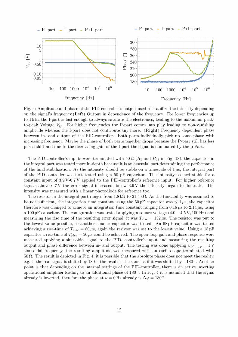
Fig. 4: Amplitude and phase of the PID-controller’s output used to stabilize the intensity dependingon the signal’s frequency.(Left) Output in dependence of the frequency. For lower frequencies upto 1 kHz the I-part is fast enough to always saturate the electronics, leading to the maximum peak-to-peak Voltage Vpp. For higher frequencies the P-part comes into play leading to non-vanishingamplitude whereas the I-part does not contribute any more. (Right) Frequency dependent phasebetween in- and output of the PID-controller. Both parts individually pick up some phase withincreasing frequency. Maybe the phase of both parts together drops because the P-part still has lessphase shift and due to the decreasing gain of the I-part the signal is dominated by the p-Part.

The PID-controller’s inputs were terminated with 50 Ω (R1 and R43 in Fig. 18), the capacitor inthe integral part was tested more in-depth because it is an essential part determining the performanceof the final stabilization. As the intensity should be stable on a timescale of 1µs, the integral partof the PID-controller was first tested using a 50 pF capacitor. The intensity seemed stable for aconstant input of 3.9 V-6.7 V applied to the PID-controller’s reference input. For higher referencesignals above 6.7 V the error signal increased, below 3.9 V the intensity began to fluctuate. Theintensity was measured with a linear photodiode for reference too.

The resistor in the integral part ranges from 1.8 kΩ to 21.4 kΩ. As the tuneability was assumed tobe not sufficient, the integration time constant using the 50 pF capacitor was ≤ 1µs, the capacitortherefore was changed to achieve an integration time constant ranging from 0.18µs to 2.14µs, usinga 100 pF capacitor. The configuration was tested applying a square voltage (4.0− 4.5 V, 100 Hz) andmeasuring the rise time of the resulting error signal, it was Trise = 132µs. The resistor was put tothe lowest value possible, so another smaller capacitor was tested. An 68 pF capacitor was testedachieving a rise-time of Trise = 80µs, again the resistor was set to the lowest value. Using a 15 pFcapacitor a rise-time of Trise = 56µs could be achieved. The open-loop gain and phase response weremeasured applying a sinusoidal signal to the PID- controller’s input and measuring the resultingoutput and phase difference between in- and output. The testing was done applying a Uin,pp = 1 Vsinusoidal frequency, the resulting amplitude was measured with an oscilloscope terminated with50 Ω. The result is depicted in Fig. 4, it is possible that the absolute phase does not meet the reality,e.g. if the real signal is shifted by 180 , the result is the same as if it was shifted by −180 . Anotherpoint is that depending on the internal settings of the PID-controller, there is an active invertingoperational amplifier leading to an additional phase of 180 . In Fig. 4 it is assumed that the signalalready is inverted, therefore the phase at ν = 0 Hz already is ∆ϕ = 180 .

12

2.3.2. Intensity Stabilization and Lattice Optics

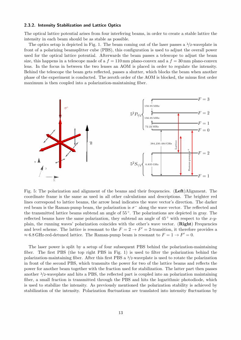
The optical lattice potential arises from four interfering beams, in order to create a stable lattice theintensity in each beam should be as stable as possible.

The optics setup is depicted in Fig. 1. The beam coming out of the laser passes a λ/2-waveplate infront of a polarizing beamsplitter cube (PBS), this configuration is used to adjust the overall powerused for the optical lattice potential. Afterwards the beam passes a telescope to adjust the beamsize, this happens in a telescope made of a f = 110 mm plano-convex and a f = 30 mm plano-convexlens. In the focus in between the two lenses an AOM is placed in order to regulate the intensity.Behind the telescope the beam gets reflected, passes a shutter, which blocks the beam when anotherphase of the experiment is conducted. The zeroth order of the AOM is blocked, the minus first ordermaximum is then coupled into a polarization-maintaining fiber.

F = 3

156.95MHz

F = 2156.95MHz

F = 172.22MHz

F = 0

52P3/2

52S1/2

384,230.484GHz

Lattice

Raman-p

umpσ+

F = 2

6.835GHz

F = 1

Fig. 5: The polarization and alignment of the beams and their frequencies. (Left)Alignment. Thecoordinate frame is the same as used in all other calculations and descriptions. The brighter redlines correspond to lattice beams, the arrow head indicates the wave vector’s direction. The darkerred beam is the Raman-pump beam, the polarization is σ− along the wave vector. The reflected andthe transmitted lattice beams subtend an angle of 55 . The polarizations are depicted in gray. Thereflected beams have the same polarization, they subtend an angle of 45 with respect to the x-y-plain, the running waves’ polarization coincides with the other’s wave vector. (Right) Frequenciesand level scheme. The lattice is resonant to the F = 2 → F ′ = 2-transition, it therefore provides a≈ 6.8 GHz-red-detuned lattice. The Raman-pump beam is resonant to F = 1→ F ′ = 0.

The laser power is split by a setup of four subsequent PBS behind the polarization-maintainingfiber. The first PBS (the top right PBS in Fig. 1) is used to filter the polarization behind thepolarization-maintaining fiber. After this first PBS a λ/2-waveplate is used to rotate the polarizationin front of the second PBS, which transmits the power for two of the lattice beams and reflects thepower for another beam together with the fraction used for stabilization. The latter part then passesanother λ/2-waveplate and hits a PBS, the reflected part is coupled into an polarization maintainingfiber, a small fraction is transmitted through the PBS and hits the logarithmic photodiode, whichis used to stabilize the intensity. As previously mentioned the polarization stability is achieved bystabilization of the intensity. Polarization fluctuations are translated into intensity fluctuations by

13

the first PBS behind the fiber since only the horizontal polarization component passes through. Thetransmitted beam after the second PBS is then split into two beams of which one is coupled into anpolarization-maintaining fiber, the other beam is guided to the chamber in free space, it is reflectedtwice and then reflected at an 50 : 50-beamsplitter, where half of the power in that beam is lost.A mirror underneath the vacuum chamber redirects the beam upwards. A λ/2-waveplate is used toalign the polarization along the transmitted beam. The beams fed into polarization-maintainingfibers are then collimated by a f = 11 mm lens in order to lead to the same beam waist as the beamentering the vacuum chamber. The beam waist directly behind the fiber collimator is w0 = 1.1 mm,for each beam the laser provides power of up to 50 mW. The polarization of the beams is adjustedby λ/2-waveplates behind the fiber collimators. The alignment is shown in Fig. 5.

The two horizontal beams, of which one is retroreflected, cross under 55 . The polarizations areset such that the two running waves both have the polarization along the other wave’s direction ofpropagation. The standing wave’s polarization encloses an angle of 55 with respect to the x-y-plain.The Raman-pump beam enters the vacuum chamber from above and is σ−-polarized. But as themagnetic field points in z-direction, which also corresponds to the atoms quantization axis, an atomeffectively experiences σ+ light.

2.4. Additional Elements used in this Experiment

To both cancel stray magnetic fields and apply linear magnetic fields in a certain direction, six coilsare mounted around the cuboid vacuum. The coils are approximately rectangular leaving a bigarea of the vacuum chamber open for optical access. The currents through the coils are driven byElektro-Automatik PS 3016-10B. Each coil has 30 windings and creates an absolute magnetic fieldper current of 0.95 G/A, 2.15 G/A and 2.30 G/A0 in x-, y- and z-direction. An additional pair ofcoils is used to create the magnetic quadrupole field during the magneto-optical trapping.

3. Explanation of a Cooling Cycle

3.1. Origin of Sidebands

To understand why a tightly-bound atom can change its motional state by a two-photon Ramantransitions we first consider an atom tightly bound in an one dimensional harmonic potential offrequency ωz/(2π). The atom is addressed by a light field E ∝ exp(i~k · ~r) + exp(−i~k · ~r), ignor-ing the time dependence, the interaction is described by 〈I,n| exp(±i~k · ~z)|I ′,n′〉, I represents theatom’s internal, n the atoms motional state. The wave vector’s projection onto the atom’s mo-tion in z-direction is given by ~k · ~z = |2π/λ| cos(θ)z = kz z, where θ is the angle between the wavevector and the z-axis [Eschner et al., 2003]. The interaction operator here represents the processof absorbing (+) or emitting (-) a photon, the atoms momentum is therefore changed by ±~kz.Introducing the motional creation and annihilation operators (cf. Equ. 57) the interaction reads〈I,n| exp(±ikz

√~/(2mωz)a+ a†)|I ′,n′〉. If the atoms ground state is much smaller than the wave

vector’s projection kzz0 = kz√

~/(2mωz) = η 1, the interaction operator can be approximated by

〈I,n|1± iη(a+ a†) +O(η2)|I ′,n′〉 ≈ δn,n′δI,I′ ± iη(√n 〈I,n|I ′,n− 1〉+

√n+ 1 〈I,n|I ′,n+ 1〉). (12)

The approximation is stringently valid if it holds that 〈Ψmotional|k2zz

2|Ψmotional〉12 1 [Wineland

et al., 1998], in an harmonic oscillator potential it yields η√n+√n2 + n 1. This limit is called

Lamb Dicke regime, it states that transitions changing the quantum number by more than ∆n = 1are strongly suppressed. The Lamb Dicke parameter can be rewritten in terms of the recoil energy

14

Erecoil = ~2k2z2m and the oscillation frequency ωz, it reads

η =

√~k2

z

2mωz=

√Erecoil~ωz

. (13)

In other words - transitions changing the motional quantum number by more than one are stronglysuppressed if the harmonic oscillator’s level spacing is large compared to the kinetic energy an atomgains if it hits a single photon. This energy is called recoil energy Erecoil. Depending on the LambDicke parameter even transitions changing the motional quantum number by one can be suppressed.

We have now seen that a tightly bound atom can only change its motional quantum number byone, therefore each internal state is dressed by a multiplet of motional states. It is assumed, thatthe internal excited state is trapped in the same manner. Assuming two states |g〉 and |e〉 withenergy difference ~ω0, and a dipole allowed transition, then the atom’s quantum state can changefrom the excited state |e〉 with motional quantum number n to the internal ground state |g〉 but themotional quantum number can change by zero or one to n, n + 1 and n − 1. The energy differenceand therefore the photon energy can then be ~ω0, ~(ω0−ωz) and ~(ω0 +ωz) for the transitions statedbefore. Therefore the central transition now shows blue and red sidebands at ω0±ωz. The motionalsidebands can only be resolved if the linewidth of the transition between the ground and excitedstate is smaller than the oscillation frequency.

3.2. The Cooling Process

The atom can be cooled in the system described above, by stimulating the atom on the red sidebandω0 − ωz. The atom then loses one quantum of kinetic energy on average if the motional quantumnumber doesn’t change on average during spontaneous emission.

The setup described above is used to implement another technique to achieve a sample of atomscooled to the 3D-motional ground state of an optical lattice. The method has been explored inan three-dimensional optical lattice by [Kerman et al., 2000] and [Treutlein et al., 2001]. PreviouslyRaman sideband cooling had been demonstrated in one- and two-dimensional optical lattices [Vuleticet al., 1998; Hamann et al., 1998]. To understand the mechanism of cooling we at first consider thesimple case, in which the optical potential for all three |F = 1,mF 〉 magnetic hyperfine levels isidentical. We than have the situation depicted in Fig. 6.

15

ℏωzn=0n=1n=2n=3n=4n=5n=6

mF=-1 mF=0 mF=1F=1

F=1

σ+

π

mF=0

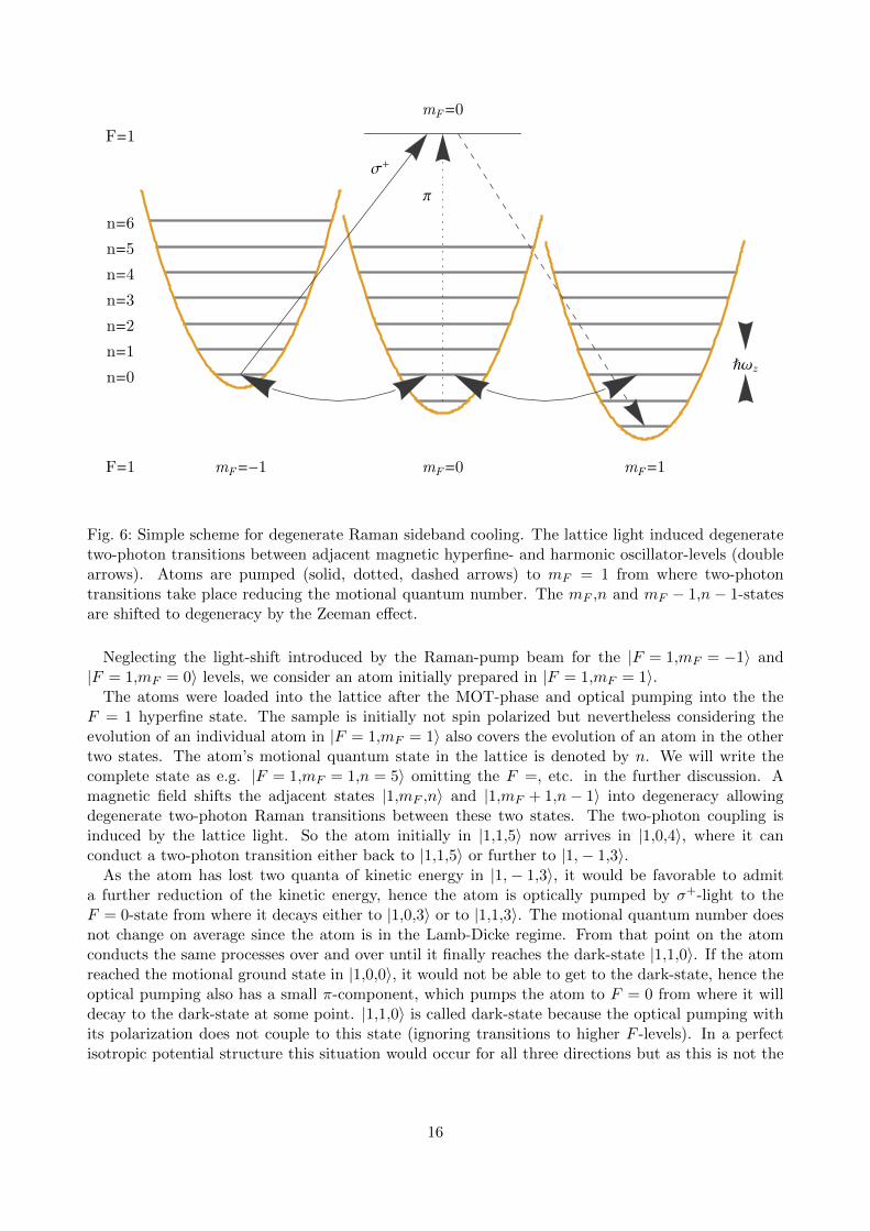
Fig. 6: Simple scheme for degenerate Raman sideband cooling. The lattice light induced degeneratetwo-photon transitions between adjacent magnetic hyperfine- and harmonic oscillator-levels (doublearrows). Atoms are pumped (solid, dotted, dashed arrows) to mF = 1 from where two-photontransitions take place reducing the motional quantum number. The mF ,n and mF − 1,n − 1-statesare shifted to degeneracy by the Zeeman effect.

Neglecting the light-shift introduced by the Raman-pump beam for the |F = 1,mF = −1〉 and|F = 1,mF = 0〉 levels, we consider an atom initially prepared in |F = 1,mF = 1〉.

The atoms were loaded into the lattice after the MOT-phase and optical pumping into the theF = 1 hyperfine state. The sample is initially not spin polarized but nevertheless considering theevolution of an individual atom in |F = 1,mF = 1〉 also covers the evolution of an atom in the othertwo states. The atom’s motional quantum state in the lattice is denoted by n. We will write thecomplete state as e.g. |F = 1,mF = 1,n = 5〉 omitting the F =, etc. in the further discussion. Amagnetic field shifts the adjacent states |1,mF ,n〉 and |1,mF + 1,n− 1〉 into degeneracy allowingdegenerate two-photon Raman transitions between these two states. The two-photon coupling isinduced by the lattice light. So the atom initially in |1,1,5〉 now arrives in |1,0,4〉, where it canconduct a two-photon transition either back to |1,1,5〉 or further to |1,− 1,3〉.

As the atom has lost two quanta of kinetic energy in |1,− 1,3〉, it would be favorable to admita further reduction of the kinetic energy, hence the atom is optically pumped by σ+-light to theF = 0-state from where it decays either to |1,0,3〉 or to |1,1,3〉. The motional quantum number doesnot change on average since the atom is in the Lamb-Dicke regime. From that point on the atomconducts the same processes over and over until it finally reaches the dark-state |1,1,0〉. If the atomreached the motional ground state in |1,0,0〉, it would not be able to get to the dark-state, hence theoptical pumping also has a small π-component, which pumps the atom to F = 0 from where it willdecay to the dark-state at some point. |1,1,0〉 is called dark-state because the optical pumping withits polarization does not couple to this state (ignoring transitions to higher F -levels). In a perfectisotropic potential structure this situation would occur for all three directions but as this is not the

16

case in the situation discussed below further assumptions are made in subsection 4.2.

4. Calculation of the Lattice Potential

4.1. Derivation of the Light-Induced Potential for a 2-Level System

The potential arises from the interaction of an atom with an electric field. In the special case ofan atom interacting with a fast oscillating electric field of light it can be explained considering atwo-level atom coupled to a classical monochromatic light-field

~E(~r, t) = Re[ ~EL(~r) exp(−iωLt)]. (14)

The resulting Hamiltonian for the atom with ground state |g〉 and excited state |e〉 reads

HA = ~ωe |e〉 〈e| , (15)

where the ground state’s energy is zero and the excited state’s energy is Ee = ~ωe. The couplingbetween the two states is created by the interaction of the atom and the field. The Hamiltonian isgiven by

HI = − ~d · ~EL(t) =~Ω

2exp(iωLt) |g〉 〈e|+

~Ω∗

2exp(−iωLt) |e〉 〈g| (16)

in the dipole-approximation, where the light’s wavelength is long compared to the extent of a single

atom, so that the field does not vary on the scale of an atom. Here ~d = −e~r denotes the transitiondipole moment. The last term assumes the rotating-wave-approximation. This approximation is validif the detuning ∆ = ωL−ωe ωe is relatively small compared to the resonant transition, this is linkedto the fact that the assumption of a two level system is valid. The coupling strength Ω = 〈g|e~r· ~EL|e〉/~,called Rabi frequency, also has to be small compared to the optical frequency |Ω| ωe, so that therotating-wave-approximation is still valid. Writing the atomic state as Ψ(t) = cg |g〉+ce |g〉, pluggingit into the Schrodinger equation

i~∂tΨ(t) = (HA + HI)Ψ(t) (17)

and using the substitution ce = ce exp(iωLt), one can obtain the resulting Hamiltonian

H = −~(ωL − ωe) |e〉 〈e|+~Ω

2|g〉 〈e|+ ~Ω∗

2|e〉 〈g| . (18)

This result can be written in matrix form, we obtain

H =

(0 ~Ω

2~Ω∗

2 −~∆

), (19)

where ∆ = ωL − ωe is the detuning from resonance. The resulting dynamics can be calculated witha density matrix

ρ =∑m,n

|m〉 ρm,n 〈n| , (20)

where 〈m| and 〈n| denote an orthonormal basis, here it reads

ρ =

(ρgg ρgeρeg ρee

)=

(|cg|2 cg c

∗e

cec∗g |ce|2

). (21)

17

Since an atom can also decay spontaneously from the excited state, additional terms are added tothe Hamiltonian, these can be derived via Weisskopf-Wigner theory of spontaneous emission [Scullyand Zubairy, 1997]. The additional Lindblad operator

L =

(Γρee −Γ

2 ρge−Γ

2 ρeg −Γρee

), (22)

describes the spontaneous decay between the excited and ground state, where Γ = ω3e |〈 ~d〉|

2

3πε0~c3 denotesthe natural line width. We assume that the rates at which the atom’s state changes act independentand can simply be added [Cohen-Tannoudji et al., 2004]. The von Neumann equation

∂tρ = − i~

[H,ρ] + L (23)

now yields four coupled differential equations, of which only 2 are independent as it holds thatρee + ρgg = 1 and ρge = ρeg∗. Therefore one has to find a solution to two coupled differentialequations.

∂tρgg = Γρee +i

2(Ω∗ρge − Ωρeg) (24)

∂tρee = −Γρee +i

2(Ωρeg − Ω∗ρge) (25)

∂tρge = −(

Γ

2+ i∆

)ρge +

i

2Ω(ρgg − ρee) (26)

∂tρeg = −(

Γ

2− i∆

)ρeg +

i

2Ω∗(ρee − ρgg) (27)

A steady state solution makes sense if the atom’s internal evolution is faster than the timescale inwhich it travels over the distance of the light’s wavelength but not for timescales in which it changesits internal state, ergo ωL t−1 max[Γ,Ω]. The steady state solution can be obtained setting thetime derivatives ∂tρi = 0,

ρee =|Ω|2

Γ2 + 4∆2 + 2|Ω|2(28)

ρge =(iΓ + 2∆)Ω

Γ2 + 4∆2 + 2|Ω|2. (29)

To derive a (conservative) force and from that on a potential, we consider a semi-classical force.Noting that ∂t~p = ~F , we can find the average force expectation value ∂t 〈p〉 with the help of theEhrenfest theorem

∂t 〈p〉 =1

i~〈[p,H]〉

= −〈[~∇,H]〉= −Tr[ρ[~∇,H]].

(30)

The Hamiltonian in this case does not only respect the atom’s internal degrees of freedom but also theexternal ones, therefore the Hamiltonian Hres consists of the spontaneous decay Hamiltonian Hspont

as well as the atom-light interaction Hamiltonian Hint and the kinetic energy term of the atom

Hres =p2

2m+ Hspont + Hint. (31)

18

We note that the momentum and position operators are now acting on the atom’s momentum andposition, therefore the electric field can depend on the position, therefore also the coupling strength.We now plug Equ. 31 into Equ. 30, it yields

〈~F 〉 = −Tr[ρ[~∇,Hint]]

= −~∇(~Ω

2

)= −~

2

[(~∇Ω(~r))ρeg + (~∇Ω∗(~r))ρge

]with Ω(~r) = |Ω(~r)| exp(iφ(~r))

= −~

(~∇|Ω(~r)|) Re[exp(iφ(~r))ρeg]− |Ω(~r)|(~∇φ(~r)) Im[exp(iφ(~r))ρeg]

Using the steady-state solutions from Equ. 29 we obtain for the semi-classical force

〈~F 〉 = −~

(∆~∇|Ω(~r)|2

Γ2 + 4∆2 + 2|Ω|2+|Ω(~r)|2Γ~∇φ(~r)

Γ2 + 4∆2 + 2|Ω|2

), (32)

we note that the time dependence is still there but its hidden in ρge. The first term correspondsto a reactive force, the second term to dissipative force since it varies with the phase of the Rabifrequency, which depends on the electric field’s phase. Another approach to derive this result would

be to consider the driven atom as having an induced dipole moment 〈 ~d〉, the resulting Potential would

then be U(~r,t) = 〈 ~d〉 ~E(~r,t). In the far-off-resonant limit Ω,Γ ∆ one can rewrite the force as

〈~F 〉 = −~

(~∇|Ω(~r)|2

4∆+|Ω(~r)|2Γ~∇φ(~r)

4∆2

). (33)

We can then find a (time averaged) potential using F = −~∇U(~r), rewriting |Ω|2 in terms of the line

width Γ and the intensity I(~r) =ε0c| ~E(~r)|2

2 , the bar denotes time averaged value, the first term reads

Udip(~r) =3πc2Γ

2ω3e∆

I(~r), (34)

where c denotes the speed of light. We see that the potential has a minimum at the maximumintensity for negative detuning and vice versa.

4.2. Resulting Lattice and Approximation

4.2.1. The Polarizability Tensor

In a real system the 2-level approximation does often not describe the full physics. An easy approachis to introduce the coupling of a (optically pumped) hyperfine ground state F to multiple hyperfineexcited states F ′ via an light-shift operator [Deutsch and Jessen, 1998]

U(~r) = ~EL(~r)∗∑F ′,mm′,m′′

|F,m〉 〈F,m| ~d |F ′,m′〉 〈F ′,m′| ~d |F,m′′〉 〈F,m′′|~∆F→F ′

~EL(~r), (35)

here ∆F→F ′ denotes the detuning from the F → F ′-transition. It is composed of the electric fieldand a polarizability tensor. This tensor contains the coupling terms between different states coupledby two photons. We can rewrite this expression in terms of reduced matrix elements, Wigner 3-j and

19

Wigner 6-j symbols separately for each polarization component σ. The common transition symbolsσ+, π and σ− correspond to σ = −1, σ = 0 and σ = 1. The Wigner 3-j symbols yield zero unless itholds that mF = m′F + q.

〈F,m|dσ|F ′,m′〉 =(−1)F−m√

2F + 1

(F 1 F ′

−m σ m′

)〈F‖ ~d‖F ′〉 (36)

=(−1)F−m+F ′+J+1+I√

(2F + 1)(2F ′ + 1)(2J + 1)

×(F 1 F ′

−m σ m′

)J J ′ 1F ′ F I

〈J‖ ~d‖J ′〉

(37)

〈F ′,m′|d−σ′ |F,m′′〉 =(−1)F′−m′+F+J ′+1+I+σ′

√(2F + 1)(2F ′ + 1)(2J + 1)

×(F ′ 1 F−m′ −σ′ m′′

)J ′ J 1F F ′ I

〈J ′‖ ~d‖J〉 .

(38)

For a component σ of a tensor operator of rank k it holds that (T(k)σ )† = (−1)σT

(k)−σ having that in

mind one can derive a link between the two reduced matrix elements from above [Steck, 2007], itfollows

〈J ′‖T (k)‖J〉 = (−1)J′−J√

2J + 1

2J ′ + 1〈J‖T (k)‖J ′〉∗ . (39)

Together with symmetries of the Wigner 6-j symbols [Edmonds, 1957] [Edmonds, 1957] [Edmonds,1957]we can write the whole expression in a more compact form

〈F,m|dσ|F ′,m′〉 〈F ′,m′|d−σ′ |F,m′′〉 =

(−1)2I+2J ′−m−m′+σ′(2F + 1)(2F ′ + 1)(2J + 1)

×(F 1 F ′

−m σ m′

)(F ′ 1 F−m′ −σ′ m′′

)J J ′ 1F ′ F I

2 ∣∣∣〈J‖ ~d‖J ′〉∣∣∣2 (40)

Note that the inversion of the second polarization term σ′ implicates that the polarization is nowalways in the same frame, e.g. a Raman transition mF → mF + 1 → mF corresponds to σ+ lightin both cases. Evaluating the sum in Equ. 35 for each polarization combination yields nine matrices(cf. Appendix B). We assume that the introduced Zeeman splitting and the splitting between theexcited hyperfine states is much smaller than the laser detuning from resonance

∆Zeman ∆HFS′ ∆. (41)

The detuning in Equ. 35 then simplifies to one fixed value ∆. The sum can be evaluated on a subspace as big as possible also taking n = 6, etc. states into account, but as we are interested in thecoupling between the |F = 1,mF 〉 levels we sum over all excited states of the 52P3/2 state and takemF and m′′F of the F = 1 ground state. This assumption is valid, if the detuning from other excitedstates is huge compared to the detuning from resonance of one specific transition. The detuning fromthe D1-line for example is in the order of THz while the detuning from the D2 line is on the order ofGHz.

An alternative representation of the light shift operator Equ. 35 in the limit of a detuning greaterthen the excited state hyperfine splitting reads

UF (~r) =

∣∣∣〈J‖ ~d‖J ′〉∣∣∣212~∆Fmax→F ′max

(2∣∣∣ ~EL(~r)

∣∣∣21 + i[ ~EL(~r)∗ × ~EL(~r)]~F

F

). (42)

20

The double bars indicate the reduced matrix element [Steck, 2001], the states Fmax describe thestretched states Fmax = I + J where I and J are the quantum numbers for nuclear spin and total

angular momentum. 1 represents the identity operator, and~FF is the (dimensionless) total spin

operator. We can see that there are off-diagonal terms in the potential (cf. Appendix B). Theseterms introduce the coupling between different magnetic hyperfine states, the potential thereforedepends on the magnetic state of the atom. The first term of UFmax(~r) can be rewritten to obtainEqu. 34 again.

Evaluating Equ. 35 for each polarization combination separately, we obtain nine three dimensionalsquare matrices for the subspace of the lower hyperfine ground state F = 1. With two-photontransitions coherences between levels with ∆mF = 0, ± 1,±2 occur, but in the limit of infinitedetuning the coherences for ∆mF = ±2 vanish. The resulting matrices are depicted in Appendix B.Calculating the transition frequencies and potentials can be done in the usual Cartesian coordinatesystem or in the spherical basis. The spherical basis vectors are made up of the Cartesian basisvectors as follows

~e+1 = − 1√2

(~ex + i~ey)

~e−1 =1√2

(~ex − i~ey)

~e0 = ~ez,

(43)

it holds that ~eq∗ = (−1)q~e−q. (44)

A vector field ~F = Fx~ex + Fy~ey + Fz~ez can be transformed to the spherical basis by a linear trans-formation F+1

F−1

F0

=1√2

−1 i 01 −i 0

0 0√

2

·FxFyFz

. (45)

Applying this transformation to the electric field we obtain the electric field components for eachpolarization. We see that the two circular polarized beams always have the same intensity at eachpoint in space, therefore the diagonal part of the resulting potential is the same for all mF states.The quantization axis points along the magnetic field in positive z-direction. The resulting potentialis calculated in the following.

4.2.2. Calculation of the Lattice Characteristics

The potential can be designed such that the potential shows a periodic structure in each direction.A simple setup could consist of four interfering beams to create a three dimensional lattice-likestructure. This resulting potential landscape is called optical lattice. The lattice described in sub-subsection 2.3.2 can not be described as aesthetic as an optical lattice derived from orthogonal beamscould be described. Nevertheless we can calculated the characteristics of that potential numerically.In principle there happen a lot of fascinating phenomena if an atom is stored in an optical lattice,e.g. an atom can tunnel through the potential barrier or it can be excited to a state which is nottrapped and simply fly away and be trapped again after a relaxation process. But as we are inter-ested in cooling a sample of atoms we will consider a regime, where we can neglect the coupling ofthe internal state and the external (movement) state. In order to motivate this approximation wewill first consider the potential produced by four interfering beams. Each beam is collimated to a1/e2 beam waist w0 = 1.1 mm and carries Pj = 50 mW of power, the laser is ∆ = −6.835 GHz de-tuned from resonance of the D2-line. To gain some intuition for the overall structure, the potential’senergy-isosurfaces are depicted in Fig. 7.

21

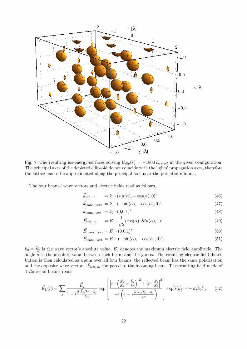
Fig. 7: The resulting iso-energy-surfaces solving Udip(~r) = −1800Erecoil in the given configuration.The principal axes of the depicted ellipsoid do not coincide with the lights’ propagation axes, thereforethe lattice has to be approximated along the principal axis near the potential minima.

The four beams’ wave vectors and electric fields read as follows,

~krefl, in = k0 · (sin(α),− cos(α), 0)τ (46)

~ktrans, horz = k0 · (− sin(α),− cos(α), 0)τ (47)

~ktrans, vert = k0 · (0,0,1)τ (48)

~Erefl, in = E0 ·1√2

(cos(α), Sin(α), 1)τ (49)

~Etrans, horz = E0 · (0,0,1)τ (50)

~Etrans, vert = E0 · (− sin(α),− cos(α), 0)τ , (51)

k0 = 2πλ is the wave vector’s absolute value, E0 denotes the maximum electric field amplitude. The

angle α is the absolute value between each beam and the y-axis. The resulting electric field distri-bution is then calculated as a sum over all four beams, the reflected beam has the same polarizationand the opposite wave vector −~krefl, in compared to the incoming beam. The resulting field made of4 Gaussian beams reads

~EL(~r) =∑j

~Ej

1− i |r·~kj/k0|−djzR

exp

∣∣∣r · ( ~Ej

E0×

~kjk0

)∣∣∣2 +∣∣∣r · ~EjE0

∣∣∣2w2

0

(1− i |r·

~kj/k0|−djzR

) exp[i(~kj · ~r − djk0)], (52)

22

where r is a matrix with x,y,z on the diagonal, dj is the distance from the beams focus, zR =πw2

0λ is the Rayleigh range and w0 the beam waist [Boyd, 2008]. The index j represents the four

beams’ indices. The distance from the focus is assumed to be the same for all three running wavesdrunning = 20 cm and the retroreflected beam travels twice that distance after the fiber collimatorergo dreflected = 40 cm.

The potential then consists of a local lattice like part and a part creating a spacial confinementin the focus of the beam. The first part has a periodic structure where the potential minima areapproximately distanced by λ along the running beams and by λ/2 along the reflected beam. Thisresult is exact for a lattice made of perpendicular beams. The resulting lattice can be plotted indifferent plains, the result is depicted in Fig. 8.

23

-2000

-1500

-1000

-500

-2000

-1500

-1000

-500

-2000

-1500

-1000

-500

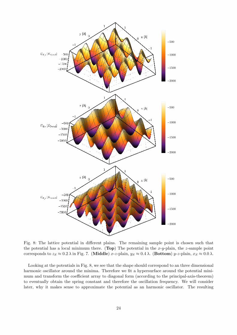
Fig. 8: The lattice potential in different plains. The remaining sample point is chosen such thatthe potential has a local minimum there. (Top) The potential in the x-y-plain, the z-sample pointcorresponds to zS ≈ 0.2λ in Fig. 7. (Middle) x-z-plain, yS ≈ 0.4λ. (Bottom) y-z-plain, xS ≈ 0.0λ.

Looking at the potentials in Fig. 8, we see that the shape should correspond to an three dimensionalharmonic oscillator around the minima. Therefore we fit a hypersurface around the potential mini-mum and transform the coefficient array to diagonal form (according to the principal-axis-theorem)to eventually obtain the spring constant and therefore the oscillation frequency. We will considerlater, why it makes sense to approximate the potential as an harmonic oscillator. The resulting

24

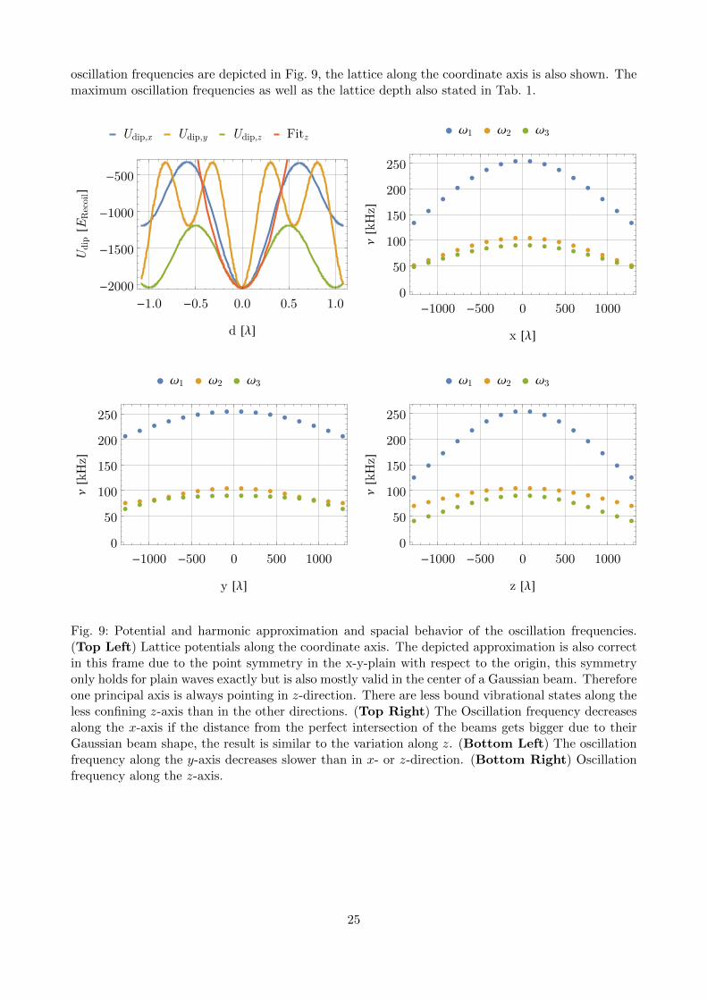
oscillation frequencies are depicted in Fig. 9, the lattice along the coordinate axis is also shown. Themaximum oscillation frequencies as well as the lattice depth also stated in Tab. 1.

Udip,x Udip,y Udip,z Fitz

-1.0 -0.5 0.0 0.5 1.0-2000

-1500

-1000

-500

d [λ]

Udi

p[E

Rec

oil]

ω1 ω2 ω3

-1000 -500 0 500 10000

50

100

150

200

250

x [λ]

ν[k

Hz]

ω1 ω2 ω3

-1000 -500 0 500 10000

50

100

150

200

250

y [λ]

ν[k

Hz]

ω1 ω2 ω3

-1000 -500 0 500 10000

50

100

150

200

250

z [λ]

ν[k

Hz]

Fig. 9: Potential and harmonic approximation and spacial behavior of the oscillation frequencies.(Top Left) Lattice potentials along the coordinate axis. The depicted approximation is also correctin this frame due to the point symmetry in the x-y-plain with respect to the origin, this symmetryonly holds for plain waves exactly but is also mostly valid in the center of a Gaussian beam. Thereforeone principal axis is always pointing in z-direction. There are less bound vibrational states along theless confining z-axis than in the other directions. (Top Right) The Oscillation frequency decreasesalong the x-axis if the distance from the perfect intersection of the beams gets bigger due to theirGaussian beam shape, the result is similar to the variation along z. (Bottom Left) The oscillationfrequency along the y-axis decreases slower than in x- or z-direction. (Bottom Right) Oscillationfrequency along the z-axis.

25

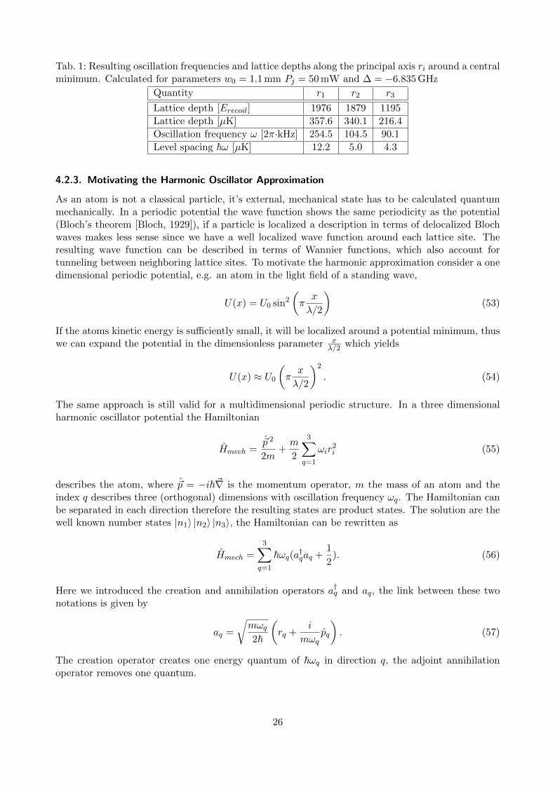
Tab. 1: Resulting oscillation frequencies and lattice depths along the principal axis ri around a centralminimum. Calculated for parameters w0 = 1.1 mm Pj = 50 mW and ∆ = −6.835 GHz

Quantity r1 r2 r3

Lattice depth [Erecoil] 1976 1879 1195

Lattice depth [µK] 357.6 340.1 216.4

Oscillation frequency ω [2π·kHz] 254.5 104.5 90.1

Level spacing ~ω [µK] 12.2 5.0 4.3

4.2.3. Motivating the Harmonic Oscillator Approximation

As an atom is not a classical particle, it’s external, mechanical state has to be calculated quantummechanically. In a periodic potential the wave function shows the same periodicity as the potential(Bloch’s theorem [Bloch, 1929]), if a particle is localized a description in terms of delocalized Blochwaves makes less sense since we have a well localized wave function around each lattice site. Theresulting wave function can be described in terms of Wannier functions, which also account fortunneling between neighboring lattice sites. To motivate the harmonic approximation consider a onedimensional periodic potential, e.g. an atom in the light field of a standing wave,

U(x) = U0 sin2

(πx

λ/2

)(53)

If the atoms kinetic energy is sufficiently small, it will be localized around a potential minimum, thuswe can expand the potential in the dimensionless parameter x

λ/2 which yields

U(x) ≈ U0

(πx

λ/2

)2

. (54)

The same approach is still valid for a multidimensional periodic structure. In a three dimensionalharmonic oscillator potential the Hamiltonian

Hmech =~p 2

2m+m

2

3∑q=1

ωir2i (55)

describes the atom, where ~p = −i~~∇ is the momentum operator, m the mass of an atom and theindex q describes three (orthogonal) dimensions with oscillation frequency ωq. The Hamiltonian canbe separated in each direction therefore the resulting states are product states. The solution are thewell known number states |n1〉 |n2〉 |n3〉, the Hamiltonian can be rewritten as

Hmech =

3∑q=1

~ωq(a†qaq +1

2). (56)

Here we introduced the creation and annihilation operators a†q and aq, the link between these twonotations is given by

aq =

√mωq2~

(rq +

i

mωqpq

). (57)

The creation operator creates one energy quantum of ~ωq in direction q, the adjoint annihilationoperator removes one quantum.

26

4.2.4. Raman Coupling

We saw in subsection 3.1 that adjacent vibrational levels are coupled by light. All beams have thesame (absolute value) wave vector. The momentum transfer after the two photon process to the atomdepends on the angle under which the photons interact with the atom. If the absorbed and emittedphoton propagate in the same direction no momentum will be transferred, while the atom gains 2~kof momentum if the emitted photon propagates in the opposite direction of the absorbed photon.We will therefore assume an average value of k, furthermore that each principal axis of a threedimensional potential minimum in the lattice couples to one beam. This beam would then stimulatetwo photon processes transferring momentum to the atoms. In principle one should consider theradiation pattern of the atom and derive an expression for the average wave vector difference butdue to the fact that we also have uncertainties in the magnetic field changing the polarization of theelectric fields the assumption of ~k will be sufficient.

We assumed that the atoms are well localized around each potential minimum, to estimate themagnitude of the coherent transitions between two levels we will calculate the electric field strengthsat a lattice minimum and sum over all couplings induced by each polarization combination. Forexample an atom in mF = 1 having (n1,n2,n3) motional quanta will be coupled to mF = 0 bycombinations of π, σ+ and σ−,π.

The electric field components in a central minimum of the lattice (Pj = 50 mW, e−2-radius =1.1 mm, ∆ = 6.835 GHz) are

E+1 = (−3763 + 3378i) V/m (58)

E−1 = (3763 + 3378i) V/m (59)

E0 = 7489 V/m. (60)

To calculate the coupling we take the results from Appendix B, as already stated we’ll consider thecoupling between mF = 1 and mF = 0.

Ucoupling =

∣∣∣〈J‖ ~d‖J ′〉∣∣∣2~∆

(E∗0 〈F = 1,mF = 1|Mπ,σ+ |F = 1,mF = 0〉E−1

+ E∗+1 〈F = 1,mF = 1|Mσ−,π|F = 1,mF = 0〉E0

)= (134 + 120i)Erecoil︸ ︷︷ ︸

from the first term

+ (134− 120i)Erecoil︸ ︷︷ ︸from the second term

= 268Erecoil

(61)

As already shown in subsection 3.1 the atom does also change its motional quantum number insome cases. The transition probability scales with the Lamb-Dicke parameter ηq and the number ofquanta in each direction nq, with the oscillation frequencies from Tab. 1 we find

η1 = 0.12

η2 = 0.19

η3 = 0.20

(62)

The sum over all three directions yields the coupling strength for transitions lowering the motionalquantum number

Ucoupling · (√n1η1 +

√n2η2 +

√n3η3) = (

√n1 · 33 +

√n2 · 51 +

√n3 · 55)Erecoil (63)

= (√n1 · 123 +

√n2 · 192 +

√n3 · 207) h · kHz, (64)

h denotes Planck’s constant. The couplings mF = 1 → m′F = 0 and mF = 0 → m′F = 1 areequal since we did not take the individual detuning between the single magnetic hyperfine states intoaccount. That fact in mind we consider the case of mF = −1→ m′F = 0. The two states get coupledby π,σ− light as well as σ+,π because this light couples to the same states like in the previous casejust with opposite sign.

27

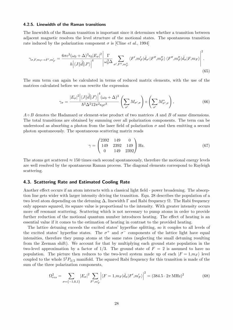
4.2.5. Linewidth of the Raman transitions

The linewidth of the Raman transition is important since it determines whether a transition betweenadjacent magnetic resolves the level structure of the motional states. The spontaneous transitionrate induced by the polarization component σ is [Cline et al., 1994]

γσ,F,mF→F ′,m′F =6πc3(ω0 + ∆)3ε0|Eσ|2

h∣∣∣〈J‖ ~d‖J ′〉∣∣∣4

∣∣∣∣∣∣ Γ

ω30∆

∑σ′,F ′′,m′′F

〈F ′,m′F |dσ′ |F ′′,m′′F 〉 〈F ′′,m′′F |dσ|F,mF 〉

∣∣∣∣∣∣2

.

(65)

The sum term can again be calculated in terms of reduced matrix elements, with the use of thematrices calculated before we can rewrite the expression

γσ =|Eσ|2

∣∣∣〈J‖ ~d‖J ′〉∣∣∣4(ω0 + ∆)3

~3∆212π2ε0c3

(∑σ′

Mσ′,σ

)

(∑σ′

M∗σ′,σ

), (66)

A B denotes the Hadamard or element-wise product of two matrices A and B of same dimensions.The total transitions are obtained by summing over all polarization components. The term can beunderstood as absorbing a photon from the laser field of polarization σ and then emitting a secondphoton spontaneously. The spontaneous scattering matrix reads

γ =

2392 149 0149 2392 1490 149 2392

Hz. (67)

The atoms get scattered ≈ 150 times each second spontaneously, therefore the motional energy levelsare well resolved by the spontaneous Raman process. The diagonal elements correspond to Rayleighscattering.

4.3. Scattering Rate and Estimated Cooling Rate

Another effect occurs if an atom interacts with a classical light field - power broadening. The absorp-tion line gets wider with larger intensity driving the transition. Equ. 28 describes the population of atwo level atom depending on the detuning ∆, linewidth Γ and Rabi frequency Ω. The Rabi frequencyonly appears squared, its square value is proportional to the intensity. With greater intensity occursmore off resonant scattering. Scattering which is not necessary to pump atoms in order to providefurther reduction of the motional quantum number introduces heating. The effect of heating is anessential value if it comes to the estimation of heating in contrast to the provided heating.

The lattice detuning exceeds the excited states’ hyperfine splitting, so it couples to all levels ofthe excited states’ hyperfine states. The σ+ and σ− components of the lattice light have equalintensities, therefore they pump atoms at the same rates (neglecting the small detuning resultingfrom the Zeeman shift). We account for that by multiplying each ground state population in thetwo-level approximation by a factor of 1/3. The ground state of F = 2 is assumed to have nopopulation. The picture then reduces to the two-level system made up of each |F = 1,mF 〉 levelcoupled to the whole 52P3/2 manifold. The squared Rabi frequency for this transition is made of thesum of the three polarization components,

Ω2res =

∑σ=−1,0,1

|Eσ|2∑F ′,m′F

∣∣∣〈F = 1,mF |dσ|F ′,m′F 〉∣∣∣2 = (384.5 · 2πMHz)2 (68)

28

The ground state population is close to unity, ≈ 0.1% of the atoms are in the excited state, resultingin a scattering rate of 4.8 · 2π kHz. Taking less restrictive assumption with the use of [Grimm et al.,2000]

Γscatter(~r) =Γ

~∆UDip(~r), (69)

we obtain a scattering rate of 6.9 · 2π kHz. From this on we can calculate the expectable heatingdue to off resonant scattering of lattice light. The heating rate depends on the one hand on the trapgeometry, on the other hand on the scattering rate and therefore also on the detuning and intensity.We assume that the heating occurs isotropic, which is not necessarily true since the absorption dueto the laser happens in specified directions, whereas spontaneous emission is isotropic. The heatingrate is discussed more in detail in [Grimm et al., 2000], it is given by

Theat =2

3

TrecΓscatter1 + κ

, (70)

where the recoil temperature is Trecoil = ~2k2/(mkB) and κ is a geometric factor, e.g. for a threedimensional harmonic trap it is κ = 1. With the values given above we obtain Theating = 827µK/s.

The levels do also shift due to the repumper, since it is resonant to F = 1 → F ′ = 0 the onlylevel affected by the (almost) pure σ+ light is the mF = −1 level. The energy eigenvalues of a lightdressed state result from diagonalizing Equ. 19, they read

Edressed± =~2

(−∆±√

∆2 + |Ω|2). (71)

If the laser is on resonance the level gets shifted by ~|Ω|/2. For the Raman-pump beam with 1 mWpower and an beam waist of 1.1 mm we obtain ΩRaman−pump = 13.9 · 2πMHz, which shifts the levelsby ~ΩRaman−pump/2 = 6.95 · hMHz.

To have a rough estimation of the scattering rate induced by the Raman-pump beam we assumethat the transition is saturated and calculate the scattering rate similar to the two level approximation

as ΓRaman−pump = 2(

ΩRaman−pumpΓ

)2· Γ

2 = 31.8 · 2πMHz. This value is an absolute upper bound of

the scattering rate for this transition since the atoms will get pumped to the other mF states. Theactual scattering rate does depend on the Raman transitions to the mF = −1 level. For reference apower of 1µW would result in an scattering rate of 31.9 kHz, which is closer to the values reportedin [Folling, 2003; Kerman et al., 2000]. The transport rate from mF = −1 to mF = 1 is by a factor1/3 smaller than the scattering rate since the relatxation from the F = 0,mF = 0 level occurs withequal probability to each of the mF ground states. Relaxation to F = 2 is neglected in this briefexplanation.

The cooling efficiency should be determined by the two-photon Raman transitions since the Raman-pumping should be chosen to be much faster than the transitions lowering the motional quantumnumber. Each Raman transition removes - in the ideal case - one quantum of kinetic energy, assumingsome mismatch and transitions between identical motional states we take half the transition ratebetween adjacent mF levels. The geometric trap frequency is ω = 3

√ω1 · ω2 · ω3 = 133.8 · 2π kHz,

together with the geometric transition frequency of νtrans = 170 kHz between adjacent mF levelswith the motional quantum numbers n and n− 1 the cooling rate results in Tcooling = 0.54 mK/s.

5. Conducted Measurements

An obvious sign of cooling nor heating was not observed to date - ipso facto the experimental stepsand measurements conducted so far will be presented.

29

5.1. Magnetic Field Nullification

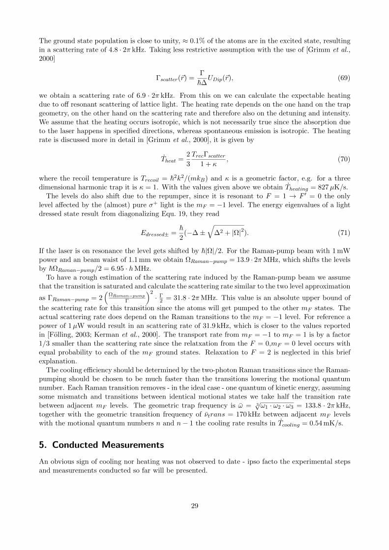
Stray magnetic fields disturb an atomic experiment due to the Zeeman effect. Therefore it is con-venient to nullify stray magnetic fields as good as possible. In the presented work this was doneutilizing microwave spectroscopy of atoms held in a far-off resonant dipole trap (ODT). The atomswere initially trapped in a magneto-optical trap and then loaded into the ODT. Subsequently theatoms were pumped to F = 1 and stored in the ODT. The population of atoms in F = 2 was probedusing single photons resonant to F = 2 → F = 3 of the D2-line. The photons were detected withLaser Components Count single photon counters.

F = 2

F = 1

mF = −2 mF = −1 mF = 0 mF = 1 mF = 2

σ−

π

σ+

σ−

π

6.835GHz

σ+

σ−

π

σ+

Fig. 10: Level scheme of a F=1→ F’=2 transition. The transition is driven by unpolarized microwaveradiation. The levels are shifted due to the linear Zeeman effect by a magnetic field along the positivequantization axis. The two hyperfine levels have a different g-factor and therefore split in oppositedirections. The individual transitions split different, therefore a variety of absorption features wasobserved. The mF = 0→ m′F = 0 does not shift with magnetic field and is a suitable starting pointwhile looking for the first signal.

The transition between the F = 1 and F = 2 hyperfine states was driven by a Anritsu MG3962C

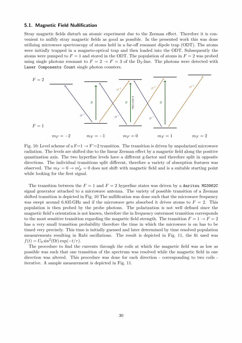
signal generator attached to a microwave antenna. The variety of possible transition of a Zeemanshifted transition is depicted in Fig. 10 The nullification was done such that the microwave frequencywas swept around 6.835 GHz and if the microwave gets absorbed it drives atoms to F = 2. Thispopulation is then probed by the probe photons. The polarization is not well defined since themagnetic field’s orientation is not known, therefore the in frequency outermost transition correspondsto the most sensitive transition regarding the magnetic field strength. The transition F = 1→ F = 2has a very small transition probability therefore the time in which the microwave is on has to betimed very precisely. This time is initially guessed and later determined by time resolved populationmeasurements resulting in Rabi oscillations. The result is depicted in Fig. 11, the fit used wasf(t) = U0 sin2(Ωt) exp(−t/τ).

The procedure to find the currents through the coils at which the magnetic field was as low aspossible was such that one transition of the spectrum was resolved while the magnetic field in onedirection was altered. This procedure was done for each direction - corresponding to two coils -iterative. A sample measurement is depicted in Fig. 11.

30

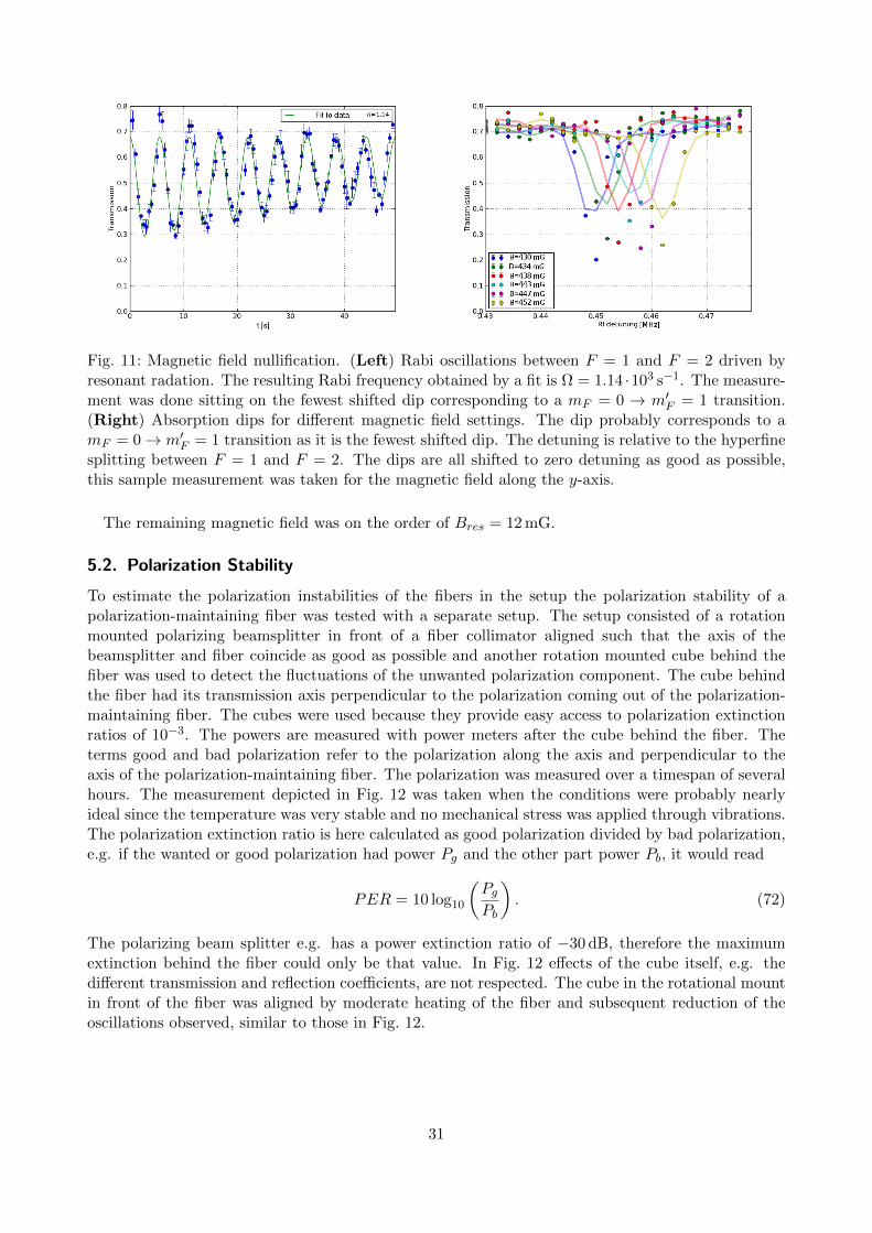
Fig. 11: Magnetic field nullification. (Left) Rabi oscillations between F = 1 and F = 2 driven byresonant radation. The resulting Rabi frequency obtained by a fit is Ω = 1.14 ·103 s−1. The measure-ment was done sitting on the fewest shifted dip corresponding to a mF = 0 → m′F = 1 transition.(Right) Absorption dips for different magnetic field settings. The dip probably corresponds to amF = 0→ m′F = 1 transition as it is the fewest shifted dip. The detuning is relative to the hyperfinesplitting between F = 1 and F = 2. The dips are all shifted to zero detuning as good as possible,this sample measurement was taken for the magnetic field along the y-axis.

The remaining magnetic field was on the order of Bres = 12 mG.

5.2. Polarization Stability

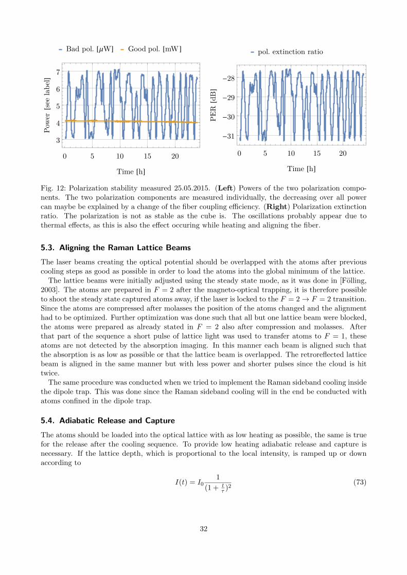
To estimate the polarization instabilities of the fibers in the setup the polarization stability of apolarization-maintaining fiber was tested with a separate setup. The setup consisted of a rotationmounted polarizing beamsplitter in front of a fiber collimator aligned such that the axis of thebeamsplitter and fiber coincide as good as possible and another rotation mounted cube behind thefiber was used to detect the fluctuations of the unwanted polarization component. The cube behindthe fiber had its transmission axis perpendicular to the polarization coming out of the polarization-maintaining fiber. The cubes were used because they provide easy access to polarization extinctionratios of 10−3. The powers are measured with power meters after the cube behind the fiber. Theterms good and bad polarization refer to the polarization along the axis and perpendicular to theaxis of the polarization-maintaining fiber. The polarization was measured over a timespan of severalhours. The measurement depicted in Fig. 12 was taken when the conditions were probably nearlyideal since the temperature was very stable and no mechanical stress was applied through vibrations.The polarization extinction ratio is here calculated as good polarization divided by bad polarization,e.g. if the wanted or good polarization had power Pg and the other part power Pb, it would read

PER = 10 log10

(PgPb

). (72)

The polarizing beam splitter e.g. has a power extinction ratio of −30 dB, therefore the maximumextinction behind the fiber could only be that value. In Fig. 12 effects of the cube itself, e.g. thedifferent transmission and reflection coefficients, are not respected. The cube in the rotational mountin front of the fiber was aligned by moderate heating of the fiber and subsequent reduction of theoscillations observed, similar to those in Fig. 12.

31

Bad pol. [μW] Good pol. [mW]

0 5 10 15 20

3

4

5

6

7

Time [h]

Powe

r[s

eela

bel]

pol. extinction ratio

0 5 10 15 20

-31

-30

-29

-28

Time [h]

PER

[dB]

Fig. 12: Polarization stability measured 25.05.2015. (Left) Powers of the two polarization compo-nents. The two polarization components are measured individually, the decreasing over all powercan maybe be explained by a change of the fiber coupling efficiency. (Right) Polarization extinctionratio. The polarization is not as stable as the cube is. The oscillations probably appear due tothermal effects, as this is also the effect occuring while heating and aligning the fiber.

5.3. Aligning the Raman Lattice Beams

The laser beams creating the optical potential should be overlapped with the atoms after previouscooling steps as good as possible in order to load the atoms into the global minimum of the lattice.

The lattice beams were initially adjusted using the steady state mode, as it was done in [Folling,2003]. The atoms are prepared in F = 2 after the magneto-optical trapping, it is therefore possibleto shoot the steady state captured atoms away, if the laser is locked to the F = 2→ F = 2 transition.Since the atoms are compressed after molasses the position of the atoms changed and the alignmenthad to be optimized. Further optimization was done such that all but one lattice beam were blocked,the atoms were prepared as already stated in F = 2 also after compression and molasses. Afterthat part of the sequence a short pulse of lattice light was used to transfer atoms to F = 1, theseatoms are not detected by the absorption imaging. In this manner each beam is aligned such thatthe absorption is as low as possible or that the lattice beam is overlapped. The retroreflected latticebeam is aligned in the same manner but with less power and shorter pulses since the cloud is hittwice.

The same procedure was conducted when we tried to implement the Raman sideband cooling insidethe dipole trap. This was done since the Raman sideband cooling will in the end be conducted withatoms confined in the dipole trap.

5.4. Adiabatic Release and Capture

The atoms should be loaded into the optical lattice with as low heating as possible, the same is truefor the release after the cooling sequence. To provide low heating adiabatic release and capture isnecessary. If the lattice depth, which is proportional to the local intensity, is ramped up or downaccording to

I(t) = I01

(1 + tτ )2

(73)

32

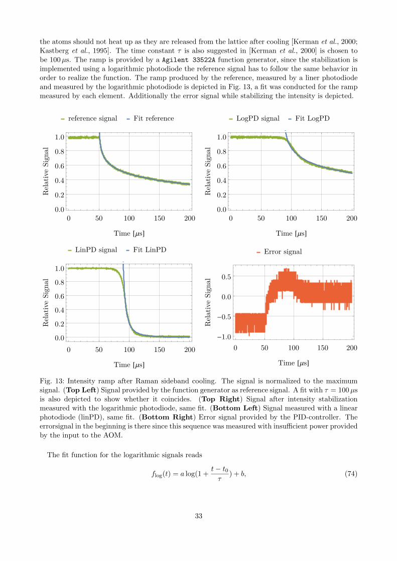
the atoms should not heat up as they are released from the lattice after cooling [Kerman et al., 2000;Kastberg et al., 1995]. The time constant τ is also suggested in [Kerman et al., 2000] is chosen tobe 100µs. The ramp is provided by a Agilent 33522A function generator, since the stabilization isimplemented using a logarithmic photodiode the reference signal has to follow the same behavior inorder to realize the function. The ramp produced by the reference, measured by a liner photodiodeand measured by the logarithmic photodiode is depicted in Fig. 13, a fit was conducted for the rampmeasured by each element. Additionally the error signal while stabilizing the intensity is depicted.

reference signal Fit reference

0 50 100 150 2000.0

0.2

0.4

0.6

0.8

1.0

Time [μs]

Rel

ativ

eSi

gnal

LogPD signal Fit LogPD

0 50 100 150 2000.0

0.2

0.4

0.6

0.8

1.0

Time [μs]

Rel

ativ

eSi

gnal

LinPD signal Fit LinPD

0 50 100 150 2000.0

0.2

0.4

0.6

0.8

1.0

Time [μs]

Rel

ativ

eSi

gnal

Error signal

0 50 100 150 200-1.0

-0.5

0.0

0.5

Time [μs]

Rel

ativ

eSi

gnal

Fig. 13: Intensity ramp after Raman sideband cooling. The signal is normalized to the maximumsignal. (Top Left) Signal provided by the function generator as reference signal. A fit with τ = 100µsis also depicted to show whether it coincides. (Top Right) Signal after intensity stabilizationmeasured with the logarithmic photodiode, same fit. (Bottom Left) Signal measured with a linearphotodiode (linPD), same fit. (Bottom Right) Error signal provided by the PID-controller. Theerrorsignal in the beginning is there since this sequence was measured with insufficient power providedby the input to the AOM.

The fit function for the logarithmic signals reads

flog(t) = a log(1 +t− t0τ

) + b, (74)

33

Tab. 2: Resulting fit parameters for functions depicted in Fig. 13

a [a.u.] b [a.u.] t0 [µs]

Reference 0.13 0.39 150

LinPD 6.75 · 10−3 −7.77 · 10−3 182

Logarithmic PD −0.16 0.51 187

whereas the function to fit to the linear photodiode’s signal was

flin(t) = a1

(1 + tτ )2

+ b. (75)

The results for the fit parameters are listed in Tab. 2.

5.5. Testing the Raman Sideband Cooling

Cooling the atomic sample which is prepared in the lattice requires all parameters to be matchedperfectly. One critical parameter is the magnetic field in order to lift the motional sidebands todegeneracy, directly associated with the magnetic field is the polarization of the Raman-pump beam.The pump beam enables this cooling technique since only atoms which are cycled have the possibilityto lower their motional quantum number n.

As a first step the polarization of the Raman-pump beam was set to be purely σ+ polarized for amagnetic field pointing along the z-axes. The cooling cycle would not work perfectly since the lastquantum could not be removed in some cases (cf. section 3). At first we adapted the polarizationsettings of [Folling, 2003], the resulting lattice is similar to the one presented in subsection 4.2, theonly difference is that the vertical running beam is polarized in y-direction. As a first approach themagnetic field along all three directions was scanned. The sequence followed in all approaches isschematically depicted in Fig. 14. The term MOT-phase corresponds to the whole procedure relatedto the magneto-optical trapping, e.g. also optical molasses and compression.

34

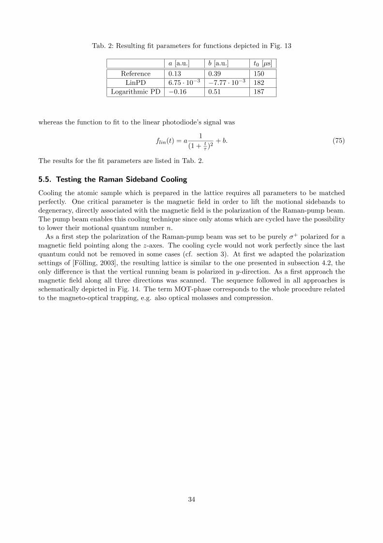
Fig. 14: Temporal sequence for Raman sideband cooling. After the MOT-phase the atoms are loadedinto the lattice and the magnetic fields are applied simultaneously. The lattice is ramped up by thefunction generator which gets a trigger pulse. The length of the cooling cycle is sent to the functiongenerator beforehand, therefore it is only triggered once. The Raman-pump beam is switched onwith little delay.

To see whether the atoms get cooled or not, they get Raman sideband cooled for 20 ms with 1 mstime of flight afterwards. After this time the atoms remaining from the MOT-phase have disappearedand only atoms which are retained in the lattice are visible to the absorption imaging. In this firstapproach the magnetic fields were scanned as follows Bx = 0 : 0,2 : 1,1 G;By = 0 : 0,4 : 2,2 G;Bz =0 : 0,4 : 2,2 G (start:step:stop). The oscillation frequencies resulting from the input power of 20 mWexpressed in form of the magnetic field necessary to lift the magnetic hyperfine levels to degeneracywere Bosc = 0.3 mG along the strongly confining and Bosc = 0.1 mG along the less confining axes.The lattice light was shut off immediately without ramping it down since we were not aiming forminimal temperature but seeing an effect of cooling. No matter which magnetic field settings wereapplied, no atoms could be retained.

Since the required magnetic fields are on the same order as the earth’s magnetic field Bearth ≈ 0.5 G[Finlay et al., 2010], the magnetic field was canceled out as good as possible (cf. subsection 5.1).Having (almost) no residual magnetic field the cooling should only depend on the magnetic field inz-direction. The magnetic field in z-direction was tested in finer steps, also both signs and thereforealso both polarizations of the Raman-pump beam were tested, but still no atoms could be retained.

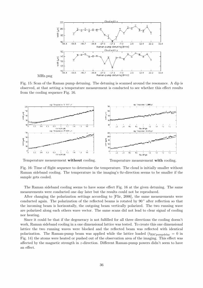
The magnetic field was then set to the theoretical value and the Raman-pump detuning wasscanned. Raman cooling was done for 5 ms with 1 ms additional time of flight. An effect was observedand the temperature with and without Raman sideband cooling was measured. The Raman-pumpdetuning exhibits a dip in the cloud widths corresponding to lower temperatures, the scan is depictedin Fig. 15.

35

MHz.png

Fig. 15: Scan of the Raman pump detuning. The detuning is scanned around the resonance. A dip isobserved, at that setting a temperature measurement is conducted to see whether this effect resultsfrom the cooling sequence Fig. 16.

Temperature measurement without cooling. Temperature measurement with cooling.

Fig. 16: Time of flight sequence to determine the temperature. The cloud is initially smaller withoutRaman sideband cooling. The temperature in the imaging’s 0x-direction seems to be smaller if thesample gets cooled.

The Raman sideband cooling seems to have some effect Fig. 16 at the given detuning. The samemeasurements were conducted one day later but the results could not be reproduced.

After changing the polarization settings according to [Flir, 2006], the same measurements wereconducted again. The polarization of the reflected beams is rotated by 90 after reflection so thatthe incoming beam is horizontally, the outgoing beam vertically polarized. The two running waveare polarized along each others wave vector. The same scans did not lead to clear signal of coolingnor heating.

Since it could be that if the degeneracy is not fulfilled for all three directions the cooling doesn’twork, Raman sideband cooling in a one dimensional lattice was tested. To create this one dimensionallattice the two running waves were blocked and the reflected beam was reflected with identicalpolarization. The Raman-pump beam was applied while the lattice loaded (tRSCpumpdelay = 0 inFig. 14) the atoms were heated or pushed out of the observation area of the imaging. This effect wasaffected by the magnetic strength in z-direction. Different Raman-pump powers didn’t seem to havean effect.

36

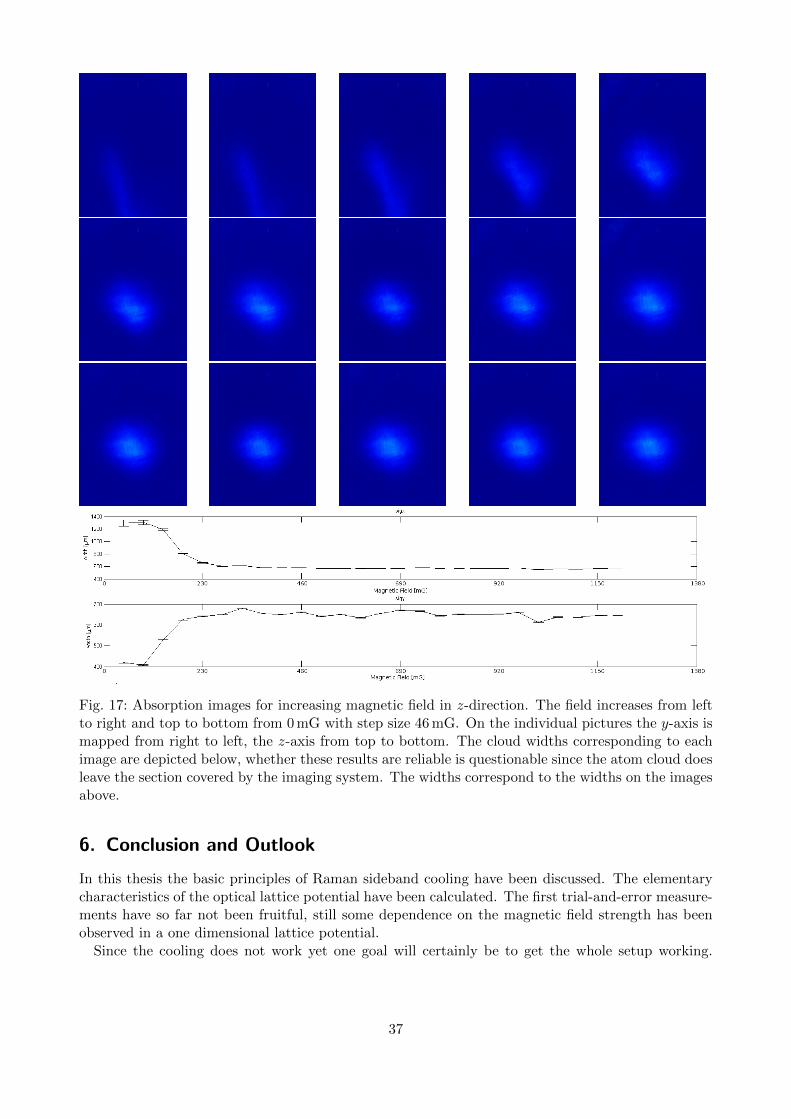
Fig. 17: Absorption images for increasing magnetic field in z-direction. The field increases from leftto right and top to bottom from 0 mG with step size 46 mG. On the individual pictures the y-axis ismapped from right to left, the z-axis from top to bottom. The cloud widths corresponding to eachimage are depicted below, whether these results are reliable is questionable since the atom cloud doesleave the section covered by the imaging system. The widths correspond to the widths on the imagesabove.

6. Conclusion and Outlook

In this thesis the basic principles of Raman sideband cooling have been discussed. The elementarycharacteristics of the optical lattice potential have been calculated. The first trial-and-error measure-ments have so far not been fruitful, still some dependence on the magnetic field strength has beenobserved in a one dimensional lattice potential.

Since the cooling does not work yet one goal will certainly be to get the whole setup working.

37

Nevertheless a setup in principle able to cool a sample of atoms to temperatures of ≈ 1µk hasbeen implemented. The time needed to cool should be on the scale of milliseconds [Folling, 2003;Kerman et al., 2000]. One key element, the Raman pump beam, maybe was chosen to have tomuch intensity introducing heating which exceeded the possible cooling rates. The provided coolingshould in principle be good enough to compensate for the scattering from the lattice. In connectionwith the overall setup which is used for quantum optical experiments it will be interesting to seedifferences in performance between Raman sideband cooling after the MOT-phase and cooling insidethe optical dipole trap. Furthermore it would be interesting to measure the trap-depth and oscillationfrequencies of the lattice and compare these to the values presented here.

38

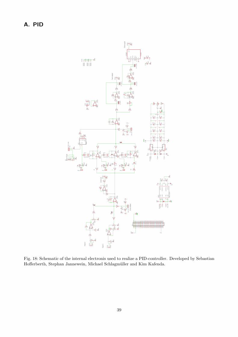
A. PID

Inpu

t 1Inpu

t 2

P I DError

offs

et

Error

out

Fast

out

put

Slo

w o

uput

Sca

n-In

put

inf

OP46

7

OP46

7

OP46

7

OP46

7

5K

inf

1K

1K

1K

10K

10K

22R

OP46

7

OP46

7

OP46

7

OP46

7

1k

ADG221KD ADG221KDADG221KD

AD

G22

1KD

56K

1K 1k

1K

1K

10K

10K

1Kinf

50k

1K

OP46

7O

P46

7

OP46

7O

P46

7

10K2uF

1K

1k02

inf

1uF

1uF

1uF

1uF

1uF

1uF

1uF

1uF

1uF

1uF

1uF

1uF

inf

1k02

781X

791X

+15V

GN

D

+15V

GN

DG

ND

2

GN

D2

10K

10K

10nF

V+ V-

GN

D2

GN

D2

GN

D2

GN

D2

GN

D2

GN

D2

GN

D2

GN

D2

GN

D2

GN

D2

GN

D2

GN

D2

GN

D2

GN

D2

GN

D2

GN

D2

GND2

20k

20k

50k

10K

0R

5k

V+

V+

V+

V-

V-

VCC

VCC

VSS

VSS

GN

D2

100n

F

1uF

1uF

1uF

1uF

GND2

GND2

In/T

estIn/T

est

Sca

n/Err

Sca

n/Err

Out

Out

GN

D2

1k

TEN

_5--12

23GND2

56KV+

100n

F

GN

D2

GN

D2

1k

1K

1K1K

10k

22R

1K

22R

22R

22R

56KGND2

V+ GN

D2

100n

F

LT10

10

V+ V-

10uF

10uF

V+

V-

GN

D2

GN

D2

GN

D2

GN

D2

GND2

DG

417

V+

V-

GND2

V+

1uF

10k

1k

GN

D2

5k GN

D2

22-2

3-20

21

22-2

3-20

31

10k

DIF

F_C

R1

231

IC1A

6 57

IC1B

9 108

IC1C

13 1214

IC1D

4 11

ER

R_O

FF1

R3

R2

R8

R9

R11

R13

R14

2 31

IC6A

6 57

IC6B

9 108

IC6C

13 1214

IC6D

4 11

R15

D 21

IC8A

S 3

D 1516

IC8B

S 14

D 109

IC8C

S 11

D7

8

IC8D

S6

13 4V+ V-5G

ND

WR

12

P-SW 1

R17

R18

R20

R25

R28

R29

R30

R32

C2

OU

T_O

FF1

123

JP-F

ASTR

332 3

1

IC11

A

6 57

IC11

B

9 108

IC11

C

13 1214

IC11

D

4 11

123

JP-F

AST2

R37

CSL

123

JP-S

LOWR

40

R41

123

JP-S

LOW

2

R43

1IN

22

C7

C9

C11

C13

C16

C17

C20

C21

C24

C25

C26

C28

C30

R38

VI

1

2

VO

3

IC2

GND

VI

2

1

VO

3

IC3

GND

C1

C2

C3

C4

C5

C6

C7

C8

C9

C10

C11

C12

C13

C14

C15

C16

C17

C18

C19

C20

C21

C22

C23

C24

C25

C26

C27

C28

C29

C30

C31

C32

J2A1

A2

A3

A4

A5

A6

A7

A8

A9

A10 A11

A12

A13

A14

A15

A16

A17

A18

A19

A20

A21

A22

A23

A24

A25

A26

A27

A28

A29

A30

A31

A32

CD

R27

R47

CI

AE

S

R48

AE

S

R50

AE

S

R51

SC

AN

_GAIN

1

R55

AE

S

R7

C37

C14

C15

C18

C10

C12

C1

C8

MO

UNT1

MO

UNT2

X1G

$1

X1G

$2X1G

$3

MO

UNT1

MO

UNT2

X2G

$1

X2G

$2

X2G

$3

MO

UNT1

MO

UNT2

X3G

$1

X3G

$2

X3G

$3

LED

R6

ZD20

-VIN

23

-VIN

12

+VIN

223

+VIN

122

+VO

UT1

14

CO

MM

ON1

9

CO

MM

ON2

16

-VO

UT2

11

PW

S1

D-SW 1

R24

C19

R57

R58

R49

R52

AE

S

R53

R26

R54

R35

R59

R60

I-SW 1

R61

C4

V+

1

BIA

S2

INPUT

8

NC_2

5

NC_3

7

NC

4

V-6

OUT

3

IC-B

UF

C5

C22

1D

2IN1

6

S1

1D1

8

GND

3V-

7

V+

4

IC4

VL

5

C3

TP1

R4

R5

AE

S

R10

1IN12

SCAN 1

PW

R-1

PW

R-2

X4-1

X4-2

X4-3

X5-1

X5-2

R12

+

+ +

15V

15V

15V

Boa

rd

Boa

rd

Boa

rd

Fig. 18: Schematic of the internal electronis used to realize a PID-controller. Developed by SebastianHofferberth, Stephan Jannewein, Michael Schlagmuller and Kim Kafenda.

39

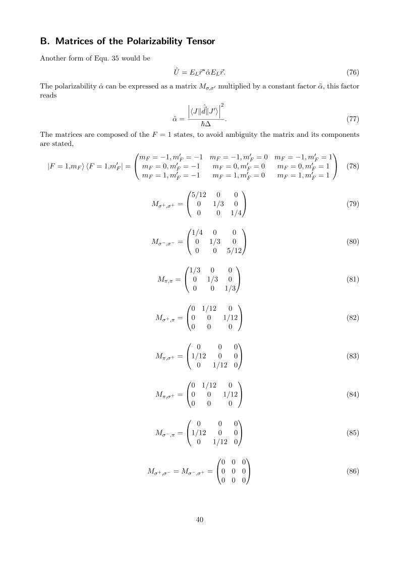
B. Matrices of the Polarizability Tensor

Another form of Equ. 35 would be

U = EL~r∗αEL~r. (76)

The polarizability α can be expressed as a matrix Mσ,σ′ multiplied by a constant factor α, this factorreads

α =

∣∣∣〈J‖ ~d‖J ′〉∣∣∣2~∆

. (77)

The matrices are composed of the F = 1 states, to avoid ambiguity the matrix and its componentsare stated,

|F = 1,mF 〉 〈F = 1,m′F | =

mF = −1,m′F = −1 mF = −1,m′F = 0 mF = −1,m′F = 1mF = 0,m′F = −1 mF = 0,m′F = 0 mF = 0,m′F = 1mF = 1,m′F = −1 mF = 1,m′F = 0 mF = 1,m′F = 1

(78)

Mσ+,σ+ =

5/12 0 00 1/3 00 0 1/4

(79)

Mσ−,σ− =

1/4 0 00 1/3 00 0 5/12

(80)

Mπ,π =

1/3 0 00 1/3 00 0 1/3

(81)

Mσ+,π =

0 1/12 00 0 1/120 0 0

(82)

Mπ,σ+ =

0 0 01/12 0 0

0 1/12 0

(83)

Mπ,σ+ =

0 1/12 00 0 1/120 0 0

(84)

Mσ−,π =

0 0 01/12 0 0

0 1/12 0

(85)

Mσ+,σ− = Mσ−,σ+ =

0 0 00 0 00 0 0

(86)

40

C. References

Appel, J., A. MacRae, and A. I. Lvovsky (2009), Measurement Science and Technology 20 (5),055302.

Bloch, F. (1929), Zeitschrift fur Physik 52 (7-8), 555.

Boyd, R. W. (2008), Nonlinear Optics (Third Edition), third edition ed. (Academic Press, Burling-ton).

Vuletic, V., C. Chin, A. J. Kerman, and S. Chu (1998), Phys. Rev. Lett. 81, 5768.

Cline, R. A., J. D. Miller, M. R. Matthews, and D. J. Heinzen (1994), Opt. Lett. 19 (3), 207.

Cohen-Tannoudji, C., J. Dupont-Roc, and G. Grynberg (2004), Atom-photon interactions: basicprocesses and applications (Wiley-VCH, Weinheim).

Deutsch, I. H., and P. S. Jessen (1998), Phys. Rev. A 57, 1972.

Edmonds, A. R. (1957), Angular momentum in quantum mechanics, Investigations in physics ; 4(Princeton Univ. Pr., Princeton, NJ).

Eschner, J., G. Morigi, F. Schmidt-Kaler, and R. Blatt (2003), J. Opt. Soc. Am. B 20 (5), 1003.

Finlay, C. C., S. Maus, C. D. Beggan, T. N. Bondar, A. Chambodut, T. A. Chernova, A. Chul-liat, V. P. Golovkov, B. Hamilton, M. Hamoudi, R. Holme, G. Hulot, W. Kuang, B. Langlais,V. Lesur, F. J. Lowes, H. Luhr, S. Macmillan, M. Mandea, S. McLean, C. Manoj, M. Menvielle,I. Michaelis, N. Olsen, J. Rauberg, M. Rother, T. J. Sabaka, A. Tangborn, L. Tøffner-Clausen,E. Thebault, A. W. P. Thomson, I. Wardinski, Z. Wei, and T. I. Zvereva (2010), GeophysicalJournal International 183 (3), 1216.

Flir, A. (2006), Implementierung und Untersuchung von Raman-Seitenbandkuhlung zur Erzeugungeines ultrakalten Casiumgases, Master’s thesis (Universitat Innsbruck).

Folling, S. (2003), 3D Raman sideband cooling of rubidium, Master’s thesis (Universitat Heidelberg).

Foot, C. J. (2005), Atomic physics, 1st ed. (Oxford University Press, Oxford).

Gerlach, W., and O. Stern (1922), Zeitschrift fur Physik 9 (1), 349.

Grimm, R., M. Weidemuller, and Y. B. Ovchinnikov (2000) (Academic Press) pp. 95 – 170.

Hamann, S. E., D. L. Haycock, G. Klose, P. H. Pax, I. H. Deutsch, and P. S. Jessen (1998), Phys.Rev. Lett. 80, 4149.

Jackson, J. D. (1982), Klassische Elektrodynamik (de Gruyter, Berlin; New York).

Kastberg, A., W. D. Phillips, S. L. Rolston, R. J. C. Spreeuw, and P. S. Jessen (1995), Phys. Rev.Lett. 74, 1542.

Kerman, A. J., V. Vuletic, C. Chin, and S. Chu (2000), Phys. Rev. Lett. 84, 439.

Scully, M. O., and M. S. Zubairy (1997), Quantum optics, 1st ed. (Cambridge University Press,Cambridge).

Steck, D. A. (2001), “Rubidium 87 d line data,” Available online at http://steck.us/alkalidata(revision 2.1.4, 23 December 2010).

41

Steck, D. A. (2007), “Quantum and atom optics,” Available online at http://steck.us/teaching

(revision 0.10.1, 30 April 2015).

Tresp, C. (2013), A Setup for Highly Precise Excitation and Detection of Rydberg Atoms, Master’sthesis (Universitat Stuttgart).

Treutlein, P., K. Y. Chung, and S. Chu (2001), Phys. Rev. A 63, 051401.

Wineland, D. J., C. Monroe, W. M. Itano, D. Leibfried, B. E. King, and D. M. Meekhof (1998), J.Research National Institute Standards Technology 103 (3), 259.

42