Implementation of biplanar coils for magnetic field generation

Miguel Maria Abreu Condessomiguel.condesso@tecnico.ulisboa.pt

Instituto Superior Tecnico, Lisboa, Portugal

May 2019

Abstract

We developed an implementation of the Target Field Method (TFM) for coil design, enabling usto obtain windings that produce a desired magnetic field, in the scope of Nuclear Magnetic Resonance(NMR). We accomplish this by minimizing a cost functional which takes into account the field pro-duced by a current distribution, as quantities that relate to the final coil’s resistance and inductance.We applied these methods to the design of a shimming set comprised of seven biplanar coils, for a gapmagnet geometry. According to simulation, the coils produce nearly orthogonal magnetic fields, withimpurities at least three to five orders of magnitude below the intensity of the dominant components.Keywords: Nuclear Magnetic Resonance, Shimming Coils, Magnetic Field, Regularization

1. Introduction

The phenomenon of Nuclear Magnetic Resonance(NMR) is based on the interaction of nuclei withstrong magnetic fields. A usually static and veryintense (0.1-10 T) magnetic field (B0) polarizes thenuclei within a sample, so that they may be probedby a second, time-varying field (B1) with a fre-quency in the radio-frequency (RF) range. The in-tensity of the field perceived by the nuclei is alteredby a number of factors, related with the kind ofmedium they are in, and how they influence eachother. The measurable response of the sample isshaped accordingly, and a great deal of informationcan be drawn from it.

The signal that arises from the response of thenuclei to the transmitted RF field is named the FreeInduction Decay (FID), which we want to optimize.The Signal-to-Noise Ratio (SNR) of the NMR ex-periment has been studied by Hoult [1]:

SNR ∝ K(B1)xyVsNB7/40 , (1)

where K is an inhomogeneity factor which, mul-tiplied by (B1)xy, the component of B1 perpen-dicular to B0, gives us the effective RF field overthe sample volume, Vs, per unit current passing inthe coil. N is the number of resonating nuclei perunit volume, so VsN is the total number of nucleicontributing to the signal. This is an intuitive re-sult: the variation ∆B0 should be minimized acrossthe Volume of Interest (VOI), so that a maximalamount of nuclei are engaged by the RF field.

There are essentially two kinds of sources of in-tensity inhomogeneities in an image obtained by

Medical Resonance Imaging (MRI): those relatedto the properties of the sample and those that con-cern the characteristics of the NMR experimentalapparatus, in which the B0 fluctuations are inserted[2]. Nuclei driven by different B0 intensities de-phase, which shortens T ∗2 locally and darkens therespective voxels. Sources of these perturbations tothe field include not only limitations in the origi-nal B0, but also distortions due to nearby materi-als with ferro-/paramagnetic properties, as well aslarge mismatches between the magnetic susceptibil-ities of the materials (e.g., water vs air) [3].

1.1. Correcting B0

One way to address the issue of undesired B0 fluc-tuations is by adding magnetic fields which opposethem – this is called shimming. There is a natu-ral distinction between passive and active shimmingmethods, because of the way they produce correc-tions to the field. We will focus our study on thelatter type, which is performed via the controlledpassage of current through specifically designed andpositioned coils. The magnetic field at r = (x, y, z)generated by a current density j along a surface Sis given by the law of Biot-Savart [4]:

B(r) = −µ0

4π

∫∫S′

(r− r′)× j(r′)

‖r− r′‖3dS′, (2)

where µ0 is the vacuum permeability and r′ aposition vector along the integration surface. Mag-netic fields can be expanded in a basis of Solid Har-monics (SH) [5], and so can their inhomogeneities.These functions form an orthonormal basis, when

1

we define an inner product which consists of anintegration over the unit sphere. Shimming coilsare usually designed as to reproduce a set of SHs(see Table 1), such that they can individually betuned in order to suppress the non-uniformities ofB0, with minimal coil coupling.

pl,m Unnormalized Expression

p0,0 1

p1,−1 y

p1,0 z

p1,1 x

p2,−2 xy

p2,−1 yz

p2,0 −x2 − y2 + 2z2

p2,1 xz

p2,2 x2 − y2

Table 1: Regular solid harmonic [5] polynomials upto the second order. The normalization constantsare cl,m = 〈 pl,m, pl,m 〉−1/2.

2. State of the art methods

In 1986, Turner [6] proposed the Target Field Method(TFM) for coil design, based on the inversion ofthe Biot-Savart law. We use this algorithm to ob-tain an appropriate current distribution, j, basedon the magnetic field we want to produce. The cur-rent density is written as a series expansion, so theproblem is reduced to finding a suitable set of coeffi-cients for the series components, Cnm. This kind ofinverse law constitutes an ill-conditioned problem,so the system must be further constrained or regu-larized, which we can do using relevant propertiesof j.

The most common approaches include Tikhonovregularization [7] and constrained optimization [8].The former relies on the addition, to the objectivefunction, of regularizing terms which account forcertain coil features. The latter consists of mini-mizing some property (e.g. low inductance) whileguaranteeing that some conditions are met (e.g. thedeviation to the target field is < 5% in the VOI).Example applications include coils with minimuminductance, for rapid switching times [9]; minimumpower consumption [10]; minimum maximum cur-rent density [11]; minimum maximum temperature[12]; acoustic noise reduction [13], among others.

2.1. Current Discretization

Having obtained the current distribution which solvesthe optimization problem, we are left with the prob-lem of discretizing j into a suitable arrangement ofcoil windings. In 1989, Edelstein and Schenck in-troduced the stream functions [14] as a simple wayof extracting the actual design of the coil from the

current density distribution that the TFM outputs.A continuous j defines a potential commonly re-ferred to as stream function ψ. The behavior of thecontinuous j is best replicated by positioning thecenter lines of the coil windings along the level setsof ψ [15]. In a planar geometry, these functions arerelated by:

j (x, y) =

(∂ψ

∂y,−∂ψ

∂x, 0

), (3)

where we have assumed that j is contained in aplane perpendicular to the z axis, so jz = 0.

2.2. Biplanar Coils

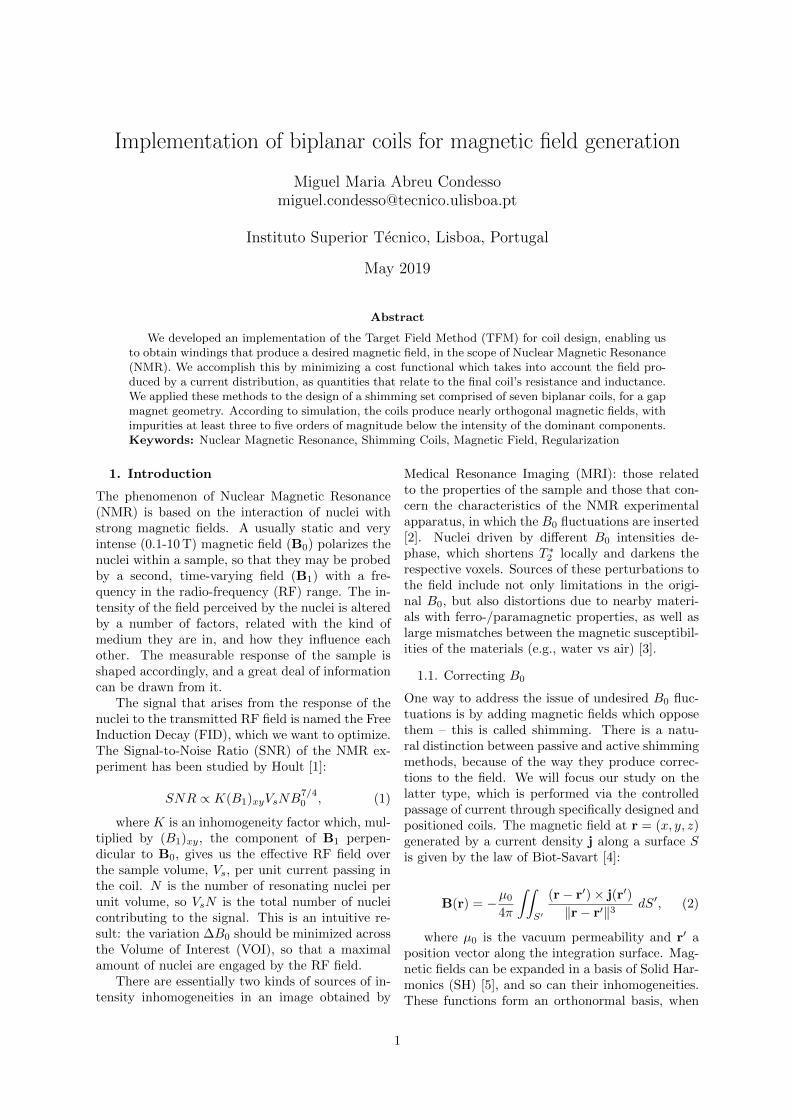
In 2004, a design strategy for shielded biplanar shimsand gradient coils was proposed by Forbes and Crozier[16]. The authors set out to find, under certainconstraints, optimal coil windings at two pairs ofplanes: primary and shielding coils (Figure 1).

Figure 1: Biplanar coil geometry from [16]. Theprimary coils are in the black planes at x = ±a,whereas the shielding coils are located at x = ±b.The target field is defined using the gray planes atx = ±c1 and x = ±c2. The outer planes, at x = ±c3are used to define the region where the field shouldbe zero, for shielding effects.

The authors defined a cost functional incorpo-rating five terms:

G = E1 + E2 + E3 + λ(a)F (a) + λ(b)F (b), (4)

where the first three measure the deviations be-tween the desired target field and the produced mag-netic field at each of the three target planes; the fol-lowing two are weighted regularization terms, i.e.,penalty functions, based on the curvature of thecoils at the primary and shielding planes, to smoothenthe winding patterns. Forbes and Crozier obtainedwindings for SHs of order 0 (constant field, see Ta-ble 1), 1 (longitudinal gradient) and 2 (xz), withand without shielding and also allowing for the coilplanes to be positioned asymmetrically.

2

2.3. Non-SH techniques

Other distinct approaches on magnetic shimmingare based on arrays of current conducting loops.Terada et al. [17] constructed a grid of connectedcircular coils and studied the inhomogeneity of Bz,in order to optimize the number of loops at each gridpoint. This kind of shimming method lacks versa-tility. Juchem et al. [18] used arrays of individuallydriven coils to produce corrective fields, allowing forsample specific corrections. The main advantage ofthese techniques is that each coil produces simplelocal corrections. This way, it is possible to handleinhomogeneities of complex shapes, without need-ing one coil for each relevant SH.

3. Implementation

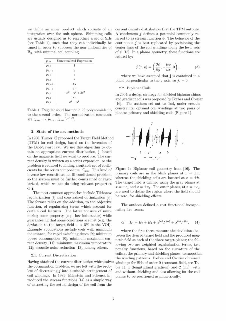
The magnetic field we are working with is producedby a gap magnet (Fig. 2). A structure holds twocylinders at a fixed distance from each other, im-posing a highly homogeneous B0 in a 15 mm gap.The structure has a high magnetic permeability, inorder to drive the magnetic flux across it, in an at-tempt to minimize flux fringing, the dispersion ofmagnetic field lines into the surrounding medium,degrading the homogeneity of the field and dimin-ishing its intensity in the gap.

B₀

(a) Gap magnet. (b) Coil Planes at z = ±a.

Figure 2: Schematic representations of the magnetsystem and the coil planes on either side of the TFV.

The approach we chose is based on a biplanar ge-ometry, as the one analyzed by Forbes and Crozierin 2004 [16]. We will place pairs of symmetricalplanar coils in the gap magnet structure (Fig. 2),in order to produce a prescribed magnetic field in aTarget Field Volume (TFV) between them.

3.1. Magnetic Field Components

We will write the current density in terms of aFourier Series, simplifying the intricate inverse prob-lem we have described into a matter of finding anadequate set of Fourier coefficients.

jx =∑n,m

CnmmLx

nLysin (n α) cos (m β)

≡∑n,m

Cnm jnmx

(5a)

jy = −∑n,m

Cnm cos (n α) sin (m β)

≡ −∑n,m

Cnm jnmy ,(5b)

where α ≡ π(x+Lx)/2Lx and β ≡ π(y+Ly)/2Ly;2Lx and 2Ly correspond to the lengths of the sidesof the coil planes. We can retrieve the magneticfield that these current density components pro-duce. They are contained in surfaces parallel tothe xy-plane, so there is no current along the z di-rection. The Biot-Savart law for the biplanar coiltakes the following form [16]:

Bnmg (r) = −µ0

2π∫∫S(±a)

(r− r′)×(jnmx (r′) , jnmy (r′) , 0

)‖r− r′‖3/2

dx′ dy′

(6)

j must be integrated at the two planes, locatedat z = ±a. The direction we choose to wind thecoils at each plane determines the kind of symmetrythat the generated field will have, as it flips thedirection of the current. For the z component, thecoils must be wound in phase to obtain an evensymmetry regarding the z axis, or counterwound incase it is odd. For the transverse components of B,even functions are achieved with counterwound coilsand odd ones by winding them in phase. We canapply the law of Biot-Savart to the current densitycomponents to find the magnetic field they produce.In eq. (7) expresses the z component of the this field,but similar expressions may be derived for the Bx

and By:

Bnmg,z (r) =

µ0

2π

∫∫S

((y − y′) jnmx − (x− x′) jnmy

)(

1

‖r− r′(+a)‖3/2+

φ

‖r− r′(−a)‖3/2

)dx′ dy′,

(7)

where the factor φ takes into account the relativedirection of the windings. Therefore, we assign φ =+1 if they are in phase, and φ = −1 if they are inphase opposition. For the total magnetic field, wesimply sum Bg(r) =

∑n,m CnmBnm

g (r).

3.2. Constructing the Target Field Method

Depending on the purpose of a particular coil, wemight want to optimize its performance taking intoaccount various properties. The inductance of gra-dient coils should be as low as possible, in orderto reach shorter switching times, allowing for fasterpulse sequences. For regular shimming coils, a typi-cal concern is resistive heating, which we can aim to

3

reduce. So our cost functional takes the followingform:

G = E + λPP + λWW, (8)

where λP and λW are regularization parameters,i.e., weights introduced to control the trade-off be-tween the field error, E, and the measures of dis-sipative power, P , and magnetic stored energy, W .We want to minimize G(Cnm), so we will require∂G

∂Cnm= 0, which results in which will result in N2

equations to solve for the N2 unknown Cnm coef-ficients. The penalty functions only contain termsthat vary either linearly with the current densitiesor quadratically. This way, we obtain a linear sys-tem to find the minimum of G.

DC = R, (9a)∑n,m

Cnm Dnmij = Rij (9b)

where D is an NxNy by NxNy matrix, and bothC and R are vectors with NxNy entries.

We define the field error term as the mean squareddifference between the target and the generated fieldwithin the TFV. The definitions for Enmij and Rij

arise from the derivatives of this term:

E =1

VTFV

∫∫∫TFV

(BT,z −∑n,m

CnmBnmg,z )2 dx dy dz

(10a)

∂E

∂Cij= 2

∑n,m

CnmEnmij + 2Rij (10b)

The dissipative power of a current density alongthe surface of a plane can be written as a surfaceintegral [19]:

P = 2ρ

t

∫S

|j|2 dS = 2ρ

t

∫S

j2x + j2y dS, (11)

where t is the thickness of the plane and ρ the re-sistivity of the material. The factor 2 is simply dueto the coils being biplanar. Using (5), the derivativeof this quantity becomes:

∂P

∂Cij= 4

ρ

t

∫S

jx∂jx∂Cij

+ jy∂jy∂Cij

dS

≡ 2∑n,m

CnmPnmij

(12)

Finally, we have the magnetic stored energy as-sociated with a current distribution [20]:

WSS′ =µ0

8π

∫S

∫S′

j(r) · j(r′) 1

‖r− r′‖dSdS′

=µ0

8π

∑n,m,k,l

CnmCkl

∫S

∫S′

1

‖r− r′‖

(jnmx jklx′ + jnm

y jkly′

)dSdS′

≡∑

n,m,i,j

CnmCij(Hnmij

x,SS′ +Hijnmx,SS′ +Hnmij

y,SS′ +Hijnmy,SS′

)(13)

Our coils are biplanar, so we need to take intoaccount not only the self-inductances of each plane(S = S′), but also their mutual inductance (S 6=S′). We can compute the derivatives of WSS′ andobtain the elements Wnmij :

∂WSS′

∂Cij=∑n,m

Cnm(Hnmijx,SS′ +Hijnm

x,SS′

+Hnmijy,SS′ +Hijnm

y,SS′)

(14a)

Wnmij = 2 Hnmijx,aa + 2 Hnmij

y,aa

+ 2φ Hnmijx,−aa + 2φ Hnmij

y,−aa

(14b)

The final elements of the matrix in the lefthandside of eq. (9a) are:

Dnmij = Enmij + λPPnmij + λWWnmij , (15)

We can assemble all of the terms and solve thelinear system for C. These solution vectors uniquelyspecify a current density distribution, that we as-sess by computing the final field error (eq. (10a)),dissipated power (eq. (11)) and magnetic stored en-ergy (using eq. (13), summing over the possible S, S′

pairs).

3.3. Current Discretization

The solution coefficients, Cnm, weigh the contribu-tion of each Fourier component, jnm, defining thecurrent distribution that produces an appropriatemagnetic field, and the corresponding stream func-tion. The current density flows along the level setsof the stream function, which correspond to the cen-ter lines of the discrete coil windings [15].

Ic = ‖maxr∈S ψ(r)−minr∈S ψ(r)

Nc‖, (16a)

ψn = minr∈S (ψ (r)) +

(n− 1

2

)Ic, n = 1, ..., Nc

(16b)

The absolute value of the current is calculatedvia eq. (16a) [15], depending on the selected number

4

of level sets, Nc. Its sign must be chosen in orderto emulate the circulation of the continuous j. Thisway, we take the contours that correspond to thelevel sets ψ = ψn, eq. (16b).

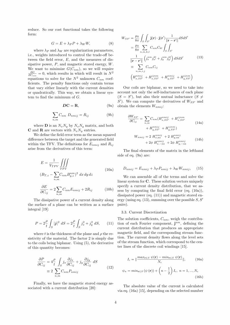
This process brings about a faithful reproduc-tion of the current distribution over the coil plane,as we can observe in Fig. 3. The discrete coun-terpart of j (Fig. 3) was constructed using a piece-wise function, which is zero-valued everywhere ex-cept along the width of the windings.

Finally, we assign physical properties to the wind-ings we have retrieved, such as width (w = 175 µm),thickness (t = 70 µm), and resistivity (Copper ρ).This way, we can evaluate the coil’s performance.First, we calculate the field error once again, butnow by applying the law of Biot-Savart to the wind-ings. We can define an inner product over the TFV:

〈 φ1, φ2 〉 =

∫∫∫TFV

φ1(r)φ2(r) dV (17)

This way, we can assess the orthogonality of thecomponents we are generating. Then, we can cal-culate the coil’s resistance:

R =ρ

w t2 ltotal (18)

where ltotal stands for the total length of thewindings at one plane. The inductance of contoursi and j can be written as:

Lij =µ0

4π

∮i

∮j

signij

dli · dlj√(xi − xj)2 + (yi − yj)2 + (zi − zj)2

,

(19)

where signij is determined for each pair of con-tours, depending on the relative phase of the currentpassing through them. The total coil inductancecan be obtained by summing through all the pos-sible i and j contours, considering that these coilsare biplanar. This incorporates both mutual andself-inductance terms.

All of the code was developed using the WolframMathematica language, and has been split into sev-eral packages. We have devised one notebook toobtain the solve the TFM and a second one wherethe solutions can be studied and discretized.

4. Results

4.1. Operation of the Target Field Method

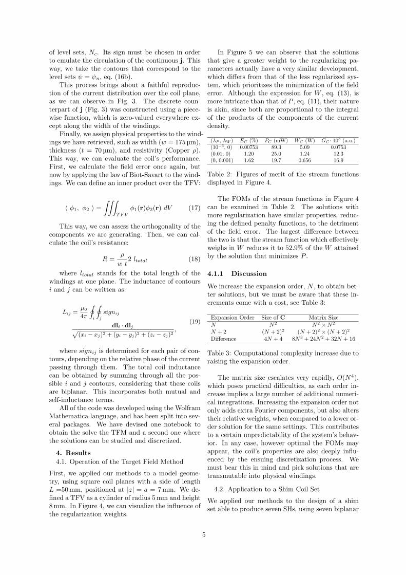
First, we applied our methods to a model geome-try, using square coil planes with a side of lengthL =50 mm, positioned at |z| = a = 7 mm. We de-fined a TFV as a cylinder of radius 5 mm and height8 mm. In Figure 4, we can visualize the influence ofthe regularization weights.

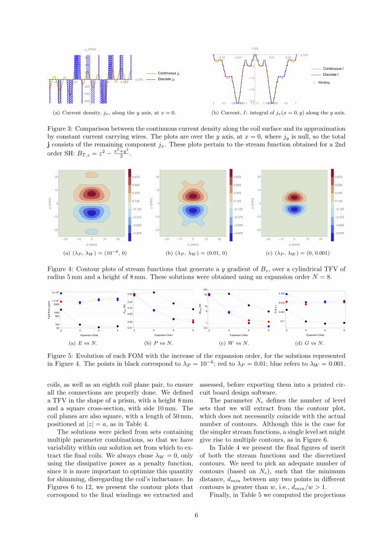
In Figure 5 we can observe that the solutionsthat give a greater weight to the regularizing pa-rameters actually have a very similar development,which differs from that of the less regularized sys-tem, which prioritizes the minimization of the fielderror. Although the expression for W , eq. (13), ismore intricate than that of P , eq. (11), their natureis akin, since both are proportional to the integralof the products of the components of the currentdensity.

(λP , λW ) EC (%) PC (mW) WC (W) GC · 103 (a.u.)(10−6, 0) 0.00753 89.3 5.09 0.0753(0.01, 0) 1.20 25.0 1.24 12.3(0, 0.001) 1.62 19.7 0.656 16.9

Table 2: Figures of merit of the stream functionsdisplayed in Figure 4.

The FOMs of the stream functions in Figure 4can be examined in Table 2. The solutions withmore regularization have similar properties, reduc-ing the defined penalty functions, to the detrimentof the field error. The largest difference betweenthe two is that the stream function which effectivelyweighs in W reduces it to 52.9% of the W attainedby the solution that minimizes P .

4.1.1 Discussion

We increase the expansion order, N , to obtain bet-ter solutions, but we must be aware that these in-crements come with a cost, see Table 3:

Expansion Order Size of C Matrix SizeN N2 N2 ×N2

N + 2 (N + 2)2 (N + 2)2 × (N + 2)2

Difference 4N + 4 8N3 + 24N2 + 32N + 16

Table 3: Computational complexity increase due toraising the expansion order.

The matrix size escalates very rapidly, O(N4),which poses practical difficulties, as each order in-crease implies a large number of additional numeri-cal integrations. Increasing the expansion order notonly adds extra Fourier components, but also alterstheir relative weights, when compared to a lower or-der solution for the same settings. This contributesto a certain unpredictability of the system’s behav-ior. In any case, however optimal the FOMs mayappear, the coil’s properties are also deeply influ-enced by the ensuing discretization process. Wemust bear this in mind and pick solutions that aretransmutable into physical windings.

4.2. Application to a Shim Coil Set

We applied our methods to the design of a shimset able to produce seven SHs, using seven biplanar

5

-0.02 -0.01 0.01 0.02y (m)

-600

-400

-200

200

400

600

jx (A/m)

Continuous jx

Discrete jx

(a) Current density, jx, along the y axis, at x = 0.

| | | | | | | | | | ||||| | | | | | | | | | | ||||| | | | | | | | | | |

-0.02 -0.01 0.01 0.02y (m)

-2.0

-1.5

-1.0

-0.5

I (A)

Continuous I

Discrete I

| Winding

(b) Current, I: integral of jx(x = 0, y) along the y axis.

Figure 3: Comparison between the continuous current density along the coil surface and its approximationby constant current carrying wires. The plots are over the y axis, at x = 0, where jy is null, so the totalj consists of the remaining component jx. These plots pertain to the stream function obtained for a 2nd

order SH: BT,z = z2 − x2+y2

2 .

-20 -10 0 10 20

-20

-10

0

10

20

x (mm)

y(mm)

-0.875

-0.625

-0.375

-0.125

0.125

0.375

0.625

0.875

(a) (λP , λW ) = (10−6, 0)

-20 -10 0 10 20

-20

-10

0

10

20

x (mm)

y(mm)

-0.875

-0.625

-0.375

-0.125

0.125

0.375

0.625

0.875

(b) (λP , λW ) = (0.01, 0)

-20 -10 0 10 20

-20

-10

0

10

20

x (mm)

y(mm)

-0.875

-0.625

-0.375

-0.125

0.125

0.375

0.625

0.875

(c) (λP , λW ) = (0, 0.001)

Figure 4: Contour plots of stream functions that generate a y gradient of Bz, over a cylindrical TFV ofradius 5 mm and a height of 8 mm. These solutions were obtained using an expansion order N = 8.

2 4 6 850

100

500

1000

5000

1×104

5×104

Expansion Order

FieldError

(ppm

)

(a) E vs N .

2 4 6 80.01

0.02

0.05

0.10

0.20

0.50

Expansion Order

Pdiss

(W)

(b) P vs N .

2 4 6 80.5

1

5

10

50

100

Expansion Order

Wmag

(W)

(c) W vs N .

2 4 6 8

10-4

0.001

0.010

0.100

Expansion Order

G(a.u.)

(d) G vs N .

Figure 5: Evolution of each FOM with the increase of the expansion order, for the solutions representedin Figure 4. The points in black correspond to λP = 10−6; red to λP = 0.01; blue refers to λW = 0.001.

coils, as well as an eighth coil plane pair, to ensureall the connections are properly done. We defineda TFV in the shape of a prism, with a height 8 mmand a square cross-section, with side 10 mm. Thecoil planes are also square, with a length of 50 mm,positioned at |z| = a, as in Table 4.

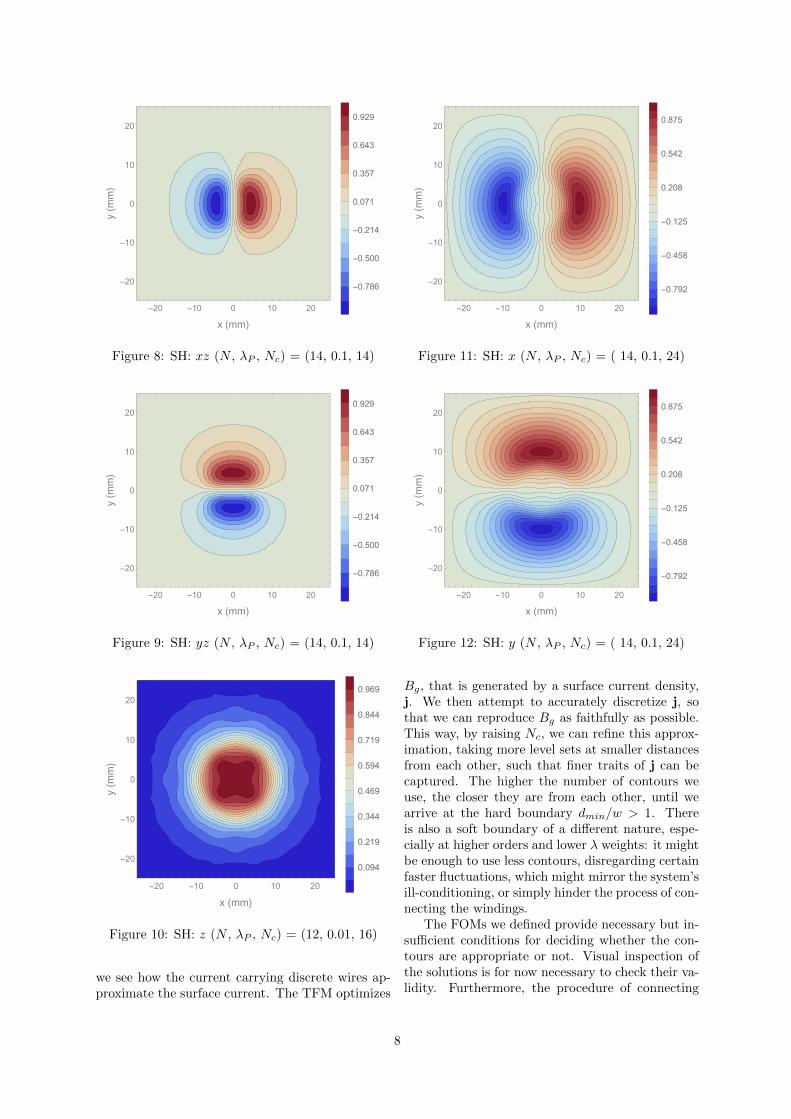
The solutions were picked from sets containingmultiple parameter combinations, so that we havevariability within our solution set from which to ex-tract the final coils. We always chose λW = 0, onlyusing the dissipative power as a penalty function,since it is more important to optimize this quantityfor shimming, disregarding the coil’s inductance. InFigures 6 to 12, we present the contour plots thatcorrespond to the final windings we extracted and

assessed, before exporting them into a printed cir-cuit board design software.

The parameter Nc defines the number of levelsets that we will extract from the contour plot,which does not necessarily coincide with the actualnumber of contours. Although this is the case forthe simpler stream functions, a single level set mightgive rise to multiple contours, as in Figure 6.

In Table 4 we present the final figures of meritof both the stream functions and the discretizedcontours. We need to pick an adequate number ofcontours (based on Nc), such that the minimumdistance, dmin between any two points in differentcontours is greater than w, i.e., dmin/w > 1.

Finally, in Table 5 we computed the projections

6

Pre-discretization Post-discretization

SH a (mm) E (%) P (mW) Nc E(%) R (Ω) L (µH) dmin/w

2nd Orderz2 −

(x2 + y2

)/2 5.819 1.04 24.9 9 0.327 3.22 6.31 1.08xy 6.039 0.0159 396 12 0.756 2.36 3.92 1.73xz 6.343 0.165 15.8 14 0.659 1.40 2.55 1.12yz 6.563 0.197 18.6 14 0.617 1.44 2.62 1.12

1st Orderz 6.867 0.159 4.59 16 0.658 3.10 9.44 1.34x 7.087 0.761 8.60 24 0.936 4.01 11.4 1.45y 7.415 0.888 9.72 24 0.881 4.05 11.5 1.45

Table 4: Figures of Merit of the selected solutions and the corresponding contours.

Shim y z x xy yz z2 xz

y 1 0 −1.70× 10−6 −4.63× 10−6 0 −7.65× 10−3 0z 0 1 0 0 1.64× 10−5 0 −1.89× 10−5

x −1.71× 10−6 0 1 −4.91× 10−6 0 8.56× 10−3 0xy −6.59× 10−5 0 −6.95× 10−5 1 0 −5.86× 10−3 0yz 0 5.27× 10−5 0 0 1 0 −2.26× 10−6

z2 −2.49× 10−3 0 2.77× 10−3 −1.34× 10−4 0 1 0xy 0 −6.10× 10−5 0 0 −2.27× 10−6 0 1

Table 5: Inner products of the fields produced by the windings over the TFV. We pick a shim field (rows,i) and project it on each of the remaining ones (columns, j): 〈Bi, Bj〉/〈Bj , Bj〉, eq. (17).

-20 -10 0 10 20

-20

-10

0

10

20

x (mm)

y(mm)

-0.944

-0.833

-0.722

-0.611

-0.500

-0.389

-0.278

-0.167

-0.056

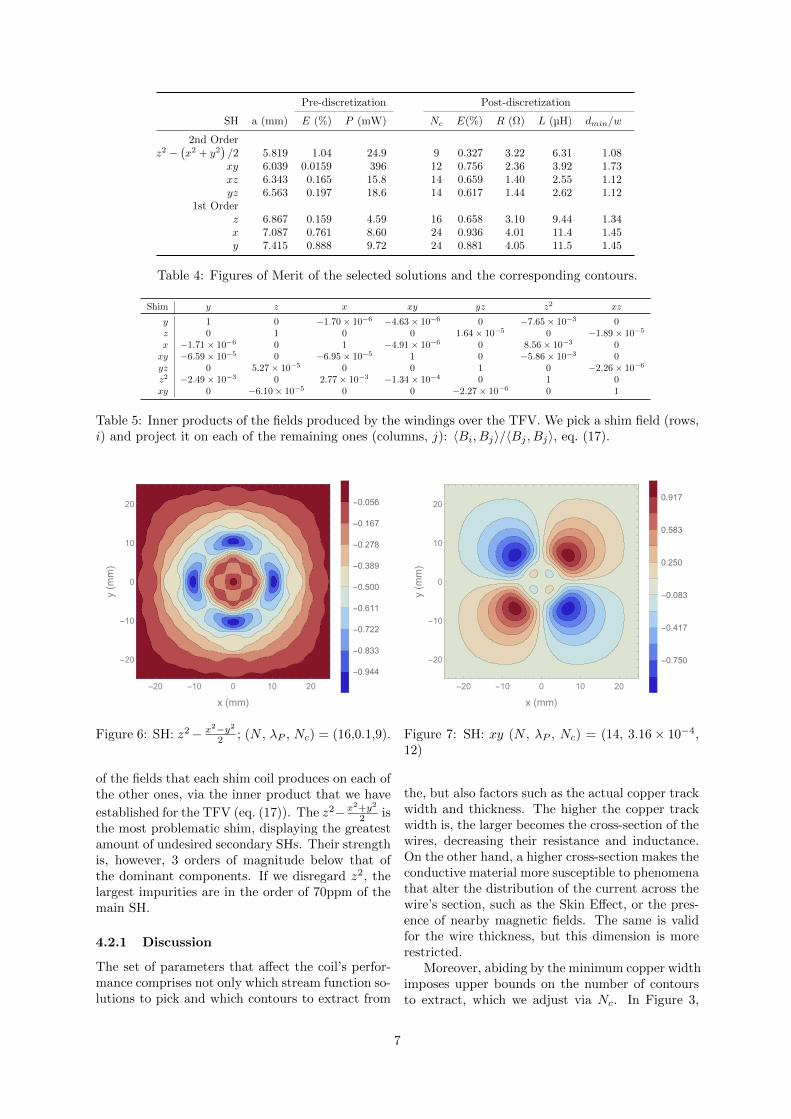
Figure 6: SH: z2− x2−y2

2 ; (N , λP , Nc) = (16,0.1,9).

of the fields that each shim coil produces on each ofthe other ones, via the inner product that we have

established for the TFV (eq. (17)). The z2−x2+y2

2 isthe most problematic shim, displaying the greatestamount of undesired secondary SHs. Their strengthis, however, 3 orders of magnitude below that ofthe dominant components. If we disregard z2, thelargest impurities are in the order of 70ppm of themain SH.

4.2.1 Discussion

The set of parameters that affect the coil’s perfor-mance comprises not only which stream function so-lutions to pick and which contours to extract from

-20 -10 0 10 20

-20

-10

0

10

20

x (mm)

y(mm)

-0.750

-0.417

-0.083

0.250

0.583

0.917

Figure 7: SH: xy (N , λP , Nc) = (14, 3.16× 10−4,12)

the, but also factors such as the actual copper trackwidth and thickness. The higher the copper trackwidth is, the larger becomes the cross-section of thewires, decreasing their resistance and inductance.On the other hand, a higher cross-section makes theconductive material more susceptible to phenomenathat alter the distribution of the current across thewire’s section, such as the Skin Effect, or the pres-ence of nearby magnetic fields. The same is validfor the wire thickness, but this dimension is morerestricted.

Moreover, abiding by the minimum copper widthimposes upper bounds on the number of contoursto extract, which we adjust via Nc. In Figure 3,

7

-20 -10 0 10 20

-20

-10

0

10

20

x (mm)

y(mm)

-0.786

-0.500

-0.214

0.071

0.357

0.643

0.929

Figure 8: SH: xz (N , λP , Nc) = (14, 0.1, 14)

-20 -10 0 10 20

-20

-10

0

10

20

x (mm)

y(mm)

-0.786

-0.500

-0.214

0.071

0.357

0.643

0.929

Figure 9: SH: yz (N , λP , Nc) = (14, 0.1, 14)

-20 -10 0 10 20

-20

-10

0

10

20

x (mm)

y(mm)

0.094

0.219

0.344

0.469

0.594

0.719

0.844

0.969

Figure 10: SH: z (N , λP , Nc) = (12, 0.01, 16)

we see how the current carrying discrete wires ap-proximate the surface current. The TFM optimizes

-20 -10 0 10 20

-20

-10

0

10

20

x (mm)

y(mm)

-0.792

-0.458

-0.125

0.208

0.542

0.875

Figure 11: SH: x (N , λP , Nc) = ( 14, 0.1, 24)

-20 -10 0 10 20

-20

-10

0

10

20

x (mm)

y(mm)

-0.792

-0.458

-0.125

0.208

0.542

0.875

Figure 12: SH: y (N , λP , Nc) = ( 14, 0.1, 24)

Bg, that is generated by a surface current density,j. We then attempt to accurately discretize j, sothat we can reproduce Bg as faithfully as possible.This way, by raising Nc, we can refine this approx-imation, taking more level sets at smaller distancesfrom each other, such that finer traits of j can becaptured. The higher the number of contours weuse, the closer they are from each other, until wearrive at the hard boundary dmin/w > 1. Thereis also a soft boundary of a different nature, espe-cially at higher orders and lower λ weights: it mightbe enough to use less contours, disregarding certainfaster fluctuations, which might mirror the system’sill-conditioning, or simply hinder the process of con-necting the windings.

The FOMs we defined provide necessary but in-sufficient conditions for deciding whether the con-tours are appropriate or not. Visual inspection ofthe solutions is for now necessary to check their va-lidity. Furthermore, the procedure of connecting

8

the windings can also represent a challenge, in caseof the more complicated coil shapes, and consid-ering that the adjacent copper planes also containcoil windings. The combination of all these effectsmakes the automation of the discretization stage acomplex task.

On another note, the orthogonality of the mag-netic fields that the shim coils produce is of greatrelevance for efficient magnetic field generation. Thez2 shim exhibits colinearity with some of the re-maining fields (Table 5) slightly below 1%. Yetthese figures are 2–3 orders of magnitude above theones registered for the other shims, so coil SH cou-pling should not represent a significant problem forthe overall efficiency of the shimming set.

5. Conclusions

We have developed a versatile implementation ofthe TFM, using the Wolfram Mathematica language.Our approach is based on a symmetrical biplanarcoil geometry and the solutions correspond to cur-rent distributions over the two coil planes. We alsodeveloped techniques for the numerical assessmentand discretization of these solutions, so that theycan be converted into actual coil windings.

We applied our work to the fabrication of a set ofshimming coils for correcting Bz, comprised of threelinear gradients (along the x, y and z directions)and four quadratic functions (xy, yz, z2−(x2−y2)/2, and xz). These coils have been built but not yettested.

The simulated magnetic fields of the coils arenearly orthogonal, displaying impurities at least 3orders of magnitude less intense than the dominantone; and 5 orders of magnitude, if we disregard z2.The shim coil set has been recently manufacturedbut it has not yet been experimentally tested dueto time constraints.

We have identified several possible directions ofimprovement for the methods we have built so far.We could expand the scope of the TFM solver byfinalizing the implementation of shielding, which isnot yet fully operational. Other than this, we cangeneralize our numerical integration methods alongthe coil planes, so that we allow the current contain-ing regions to have other geometries. For instancein MRI it is common to use coils that are cast incylindrical surfaces.

As for the discretization process, there are mainlytwo sections with room for enhancement. Firstly,we recognized that the contour selection processcurrently relies heavily on the visual inspection ofthe contour plots. In order to make this step moreefficient, we could, for instance, quantify the curva-ture of the stream functions. We could then use itto set a threshold, above which we could automati-cally rule out solutions which are already too irreg-

ular to be considered for discretization. Finally, weperform the step of joining the individual contoursinto a single connected coil in a manual way, suchthat the windings are deformed minimally, which isa common approach. However, this procedure canalso be subject of research, whether by involving asecond optimization process, or by integrating thediscretization in the TFM.

Acknowledgements

This work was developed at and received financialsupport from the Institute of Microstructure Tech-nology (IMT) at the Karlsruhe Institute of Tech-nology (KIT).

References

[1] D.I. Hoult et al. The signal-to-noise ratio of the nuclearmagnetic resonance experiment. Journal of MagneticResonance, 24(1), 1976.

[2] U. Vovk et al. A Review of Methods for Correction ofIntensity Inhomogeneity in MRI. IEEE Transactionson Medical Imaging, 26(3), 2007.

[3] Keith Wachowicz. Evaluation of active and passiveshimming in magnetic resonance imaging. Research andReports in Nuclear Medicine, 4, 2014.

[4] David J. Griffiths. Introduction to electrodynamics (3rdEdition). Prentice-Hall, 1999.

[5] E. O. Steinborn and K. Ruedenberg. Rotation andtranslation of regular and irregular solid spherical har-monics. In Advances in quantum chemistry, volume 7,pages 1–81. Elsevier, 1973.

[6] R Turner. A target field approach to optimal coil design.Journal of Physics D: Applied Physics, 19(8), 1986.

[7] Michael S. Poole et al. Convex optimisation of gradientand shim coil winding patterns. Journal of MagneticResonance, 244, 2014.

[8] Peter T. While et al. Theoretical design of gradientcoils with minimum power dissipation: Accounting forthe discretization of current density into coil windings.Journal of Magnetic Resonance, 235, 2013.

[9] M Engelsberg et al. Minimum inductance coils. Journalof Physics E: Scientific Instruments, 21, 1988.

[10] D.I. Hoult et al. Accurate Shim-Coil Designand Magnet-Field Profiling by a Power-Minimization-Matrix Method. Journal of Magnetic Resonance, SeriesA, 108, 1994.

[11] Michael Poole et al. Minimax current density coil de-sign. Journal of Physics D: Applied Physics, 43, 2010.

[12] P. T. While et al. Minimum maximum temperaturegradient coil design. Magn. Reson. Med., 70, 2013.

[13] J. M. Jackson et al. Tikhonov regularization approachfor acoustic noise reduction in an asymmetric, self-shielded mri gradient coil. Concepts Magn. Reson., 37B,2010.

[14] W. Edelstein et al. Current Streamline Method for CoilConstruction. US Patent 4840700, 1989.

[15] G. N. Peeren. Stream function approach for determin-ing optimal surface currents. Journal of ComputationalPhysics, 191, 2003.

[16] Larry K. Forbes and Stuart Crozier. Novel Target-FieldMethod for Designing Shielded Biplanar Shim and Gra-dient Coils. IEEE Transactions on Magnetics, 40(4),2004.

9

[17] Y. Terada et al. Magnetic field shimming of a perma-nent magnet using a combination of pieces of permanentmagnets and a single-channel shim coil for skeletal ageassessment of children. Journal of Magnetic Resonance,230, 2013.

[18] C. Juchem et al. B0 magnetic field homogeneity andshimming for in vivo magnetic resonance spectroscopy.Analytical Biochemistry, 529, 2016.

[19] Michael Poole et al. Novel gradient coils designed usinga boundary element method. Concepts Magn. Reson.,31B, 2007.

[20] R. A. Lemdiasov et al. A stream function method forgradient coil design. Concepts Magn. Reson., 26B, 2005.

10