Embed Size (px)
Citation preview
HAL Id: hal-00100402https://hal.archives-ouvertes.fr/hal-00100402
Submitted on 26 Sep 2006
HAL is a multi-disciplinary open accessarchive for the deposit and dissemination of sci-entific research documents, whether they are pub-lished or not. The documents may come fromteaching and research institutions in France orabroad, or from public or private research centers.
L’archive ouverte pluridisciplinaire HAL, estdestinée au dépôt et à la diffusion de documentsscientifiques de niveau recherche, publiés ou non,émanant des établissements d’enseignement et derecherche français ou étrangers, des laboratoirespublics ou privés.
Implementation of path following techniques into thefinite element code LAGAMINE
Panagiotis Kotronis, Frédéric Collin
To cite this version:Panagiotis Kotronis, Frédéric Collin. Implementation of path following techniques into the finiteelement code LAGAMINE. [Research Report] Rapport Interne Géomac/3S-R. 2005. �hal-00100402�
Internal report GeomaC/3S, September 2005
IMPLEMENTATION OF PATH FOLLOWING TECHNIQUES
INTO THE FINITE ELEMENT CODE LAGAMINE
P. KOTRONIS AND F. COLLIN
Abstract. This report presents a study on existing advanced incremental-iterative solution techniques for geometrically and physically non-linear analy-sis and their implementation into the finite element code LAGAMINE. Aftera theoretical presentation of different path following techniques, a general al-
gorithm and details about the specific implementation into LAGAMINE fol-low. Challenging examples show the advantages but also the efficiency of eachmethod.
1. Introduction
Geometrically or physically non-linear problems are often characterized by thepresence of critical points with snapping behavior in the structural response. Con-ventional Newton-type iterative strategies hold the load parameter constant whilstiterating to convergence and thus often fail to reproduce structural or materialinstabilities. This report presents a study on existing automatic following pathtechniques and their implementation into the finite element code LAGAMINE (fi-nite element code developed at the department ’GEOMAC’ of the University ofLiege under the direction of Prof. R. Charlier).
2. Newton-Raphson Procedure
2.1. An Incremental-Iterative Strategy ? The classical finite element dis-cretization process yields the following set of simultaneous equations [5],[20],[44]:
(2.1) [K] {δ} = {Fext} ,
where for structural analysis [K] is the stiffness matrix, {δ} is the vector of DOF(degrees of freedom) and {Fext} the vector of applied loads. If the stiffness matrix[K] is itself a function of the DOF values (or their derivatives) then eq.(2.1) is anonlinear equation. The Newton-Raphson method is an iterative process of solvingthe nonlinear equations and can be written as:
(2.2)[
Ktg]j−1
{∆δ}j
= {Fext} − {Fint}j−1
,
(2.3) {δ}j
= {δ}j−1
+ {∆δ}j,
Key words and phrases. arc-length method, snap-back, snap-through, bifurcation, non-uniqueness, geometrically and physically non-linear analysis, path following technique, automatedsolution control .
Panagiotis KOTRONIS is grateful for the FNRS (Fonds National pour la Recherche Scientifique- Belgium) research fellowship obtained for his two month visit at the department ’GEOMAC’ of
the University of Liege.
1
2 P. KOTRONIS AND F. COLLIN
where [Ktg]j−1
is the tangent stiffness matrix, j is the subscript representing the
equilibrium iteration and {Fint}j−1
is the vector of restoring loads corresponding
to the element internal loads. Both [Ktg]j−1
and {Fint}j−1
are evaluated based
on the values given by {δ}j−1
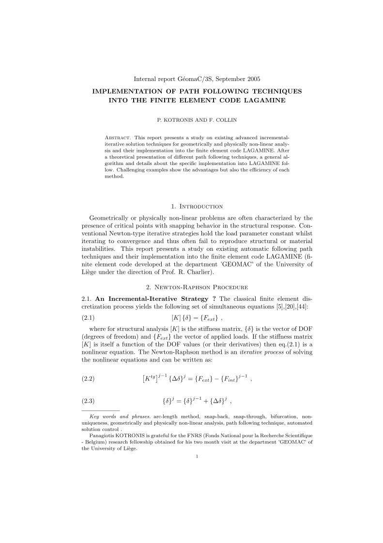
. The right-hand side of eq.(2.2) is the residual orout-of-balance load vector; i.e., the amount the system is out of equilibrium. Asingle solution iteration for a one DOF model is depicted in Figure 1.
Figure 1. Newton-Raphson procedure: One iteration for a prob-lem with a single DOF.
It is obvious that more than one iteration is needed in order to obtain a convergedsolution. The general algorithm proceeds as follows [2], Figure 2:
(1) Compute the updated tangent stiffness matrix [Ktg]j−1
and the internal
loads {Fint}j−1
from configuration {δ}j−1
;
(2) Calculate {∆δ}j
from eq.(2.2);
(3) Add {∆δ}j
to {δ}j−1
in order to obtain the next approximation {δ}j
fromeq.(2.3);
(4) Repeat steps 1 to 4 until convergence is obtained.
The solution obtained at the end of the iteration process would correspond toload level {Fext}. The final converged solution would be in equilibrium, such that
the internal loads vector {Fint}j−1
would equal to the applied load vector {Fext}(or at least within some tolerance). None of the intermediate solutions would be inequilibrium.
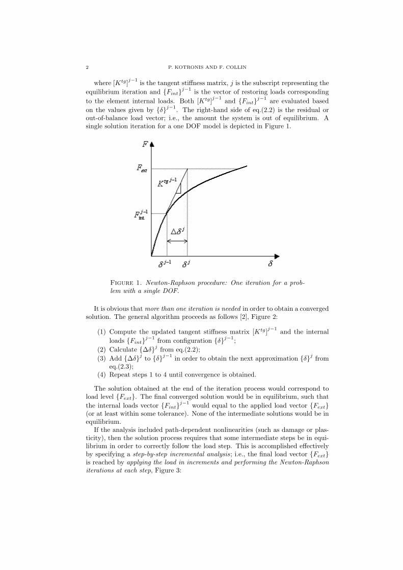
If the analysis included path-dependent nonlinearities (such as damage or plas-ticity), then the solution process requires that some intermediate steps be in equi-librium in order to correctly follow the load step. This is accomplished effectivelyby specifying a step-by-step incremental analysis; i.e., the final load vector {Fext}is reached by applying the load in increments and performing the Newton-Raphsoniterations at each step, Figure 3:
3
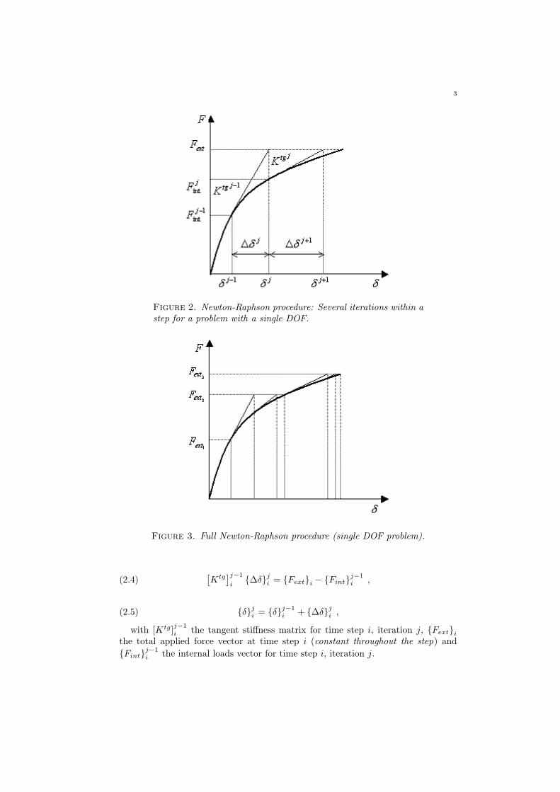
Figure 2. Newton-Raphson procedure: Several iterations within astep for a problem with a single DOF.
Figure 3. Full Newton-Raphson procedure (single DOF problem).
(2.4)[
Ktg]j−1
i{∆δ}
j
i = {Fext}i − {Fint}j−1
i ,
(2.5) {δ}j
i = {δ}j−1
i + {∆δ}j
i ,
with [Ktg]j−1
i the tangent stiffness matrix for time step i, iteration j, {Fext}i
the total applied force vector at time step i (constant throughout the step) and
{Fint}j−1
i the internal loads vector for time step i, iteration j.
4 P. KOTRONIS AND F. COLLIN
The Newton-Raphson procedure guarantees convergence if and only if the so-
lution at any iteration {δ}j
i is ‘near’ the exact solution. Therefore, even withoutpath-dependent nonlinearity, the incremental approach (i.e., applying the loads inincrements) is sometimes required in order to obtain a solution corresponding tothe final load level. That is the reason why the Newton-Raphson procedure belongsto the family of Incremental-Iterative Strategies.
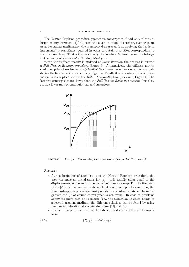
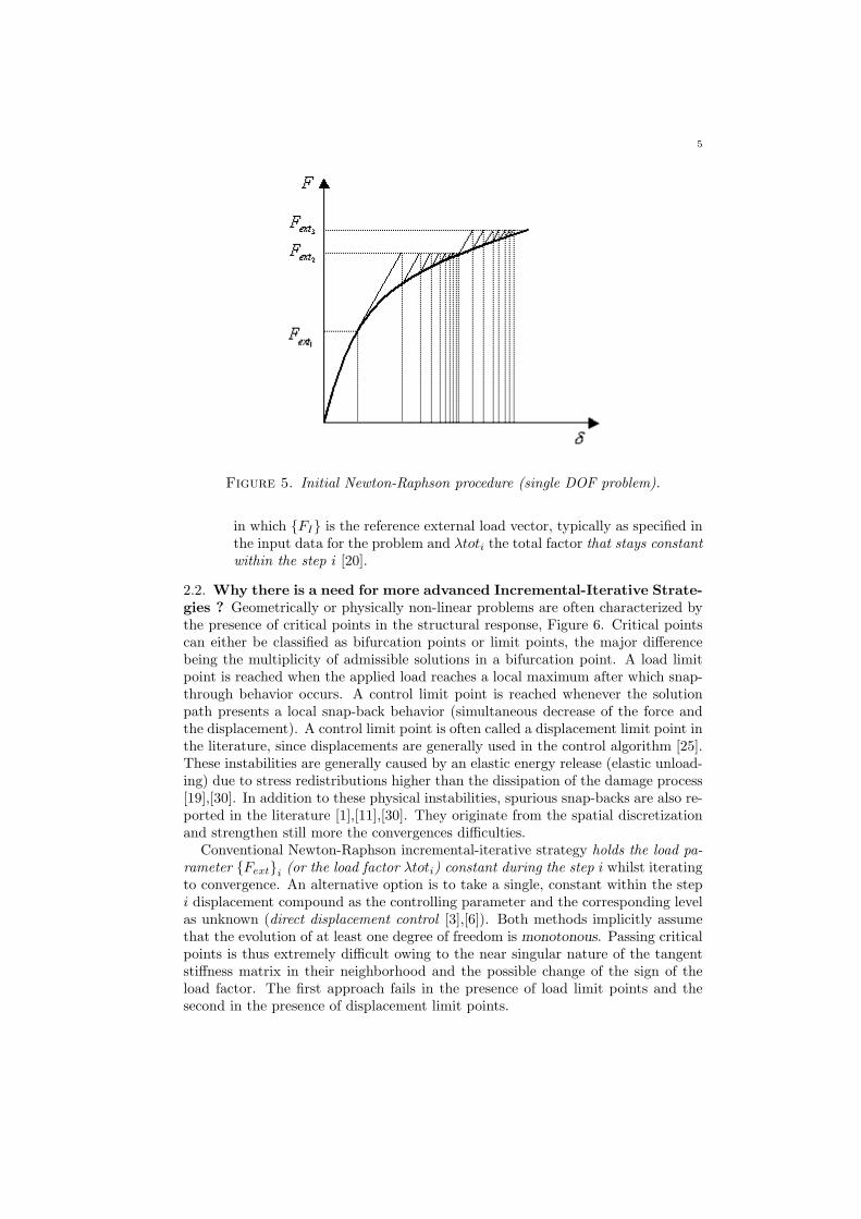
When the stiffness matrix is updated at every iteration the process is termeda Full Newton-Raphson procedure, Figure 3. Alternatively, the stiffness matrixcould be updated less frequently (Modified Newton-Raphson procedure), for exampleduring the first iteration of each step, Figure 4. Finally if no updating of the stiffnessmatrix is taken place one has the Initial Newton-Raphson procedure, Figure 5. Thelast two converged more slowly than the Full Newton-Raphson procedure, but theyrequire fewer matrix manipulations and inversions.
Figure 4. Modified Newton-Raphson procedure (single DOF problem).
Remarks:
• At the beginning of each step i of the Newton-Raphson procedure, theuser can make an initial guess for {δ}
0(it is usually taken equal to the
displacements at the end of the converged previous step. For the first step{δ}
0={0}). For numerical problems having only one possible solution, the
Newton-Raphson procedure must provide this solution whatever the initialguesses are (if of course convergence is achieved). In case of problemsadmitting more that one solution (i.e., the formation of shear bands ina second gradient medium) the different solutions can be found by usingrandom initialization at certain steps (see [12] and [13]).
• In case of proportional loading the external load vector takes the followingform:
(2.6) {Fext}i = λtoti {FI}
5
Figure 5. Initial Newton-Raphson procedure (single DOF problem).
in which {FI} is the reference external load vector, typically as specified inthe input data for the problem and λtoti the total factor that stays constantwithin the step i [20].
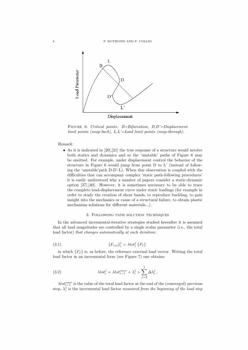
2.2. Why there is a need for more advanced Incremental-Iterative Strate-gies ? Geometrically or physically non-linear problems are often characterized bythe presence of critical points in the structural response, Figure 6. Critical pointscan either be classified as bifurcation points or limit points, the major differencebeing the multiplicity of admissible solutions in a bifurcation point. A load limitpoint is reached when the applied load reaches a local maximum after which snap-through behavior occurs. A control limit point is reached whenever the solutionpath presents a local snap-back behavior (simultaneous decrease of the force andthe displacement). A control limit point is often called a displacement limit point inthe literature, since displacements are generally used in the control algorithm [25].These instabilities are generally caused by an elastic energy release (elastic unload-ing) due to stress redistributions higher than the dissipation of the damage process[19],[30]. In addition to these physical instabilities, spurious snap-backs are also re-ported in the literature [1],[11],[30]. They originate from the spatial discretizationand strengthen still more the convergences difficulties.
Conventional Newton-Raphson incremental-iterative strategy holds the load pa-rameter {Fext}i (or the load factor λtoti) constant during the step i whilst iteratingto convergence. An alternative option is to take a single, constant within the stepi displacement compound as the controlling parameter and the corresponding levelas unknown (direct displacement control [3],[6]). Both methods implicitly assumethat the evolution of at least one degree of freedom is monotonous. Passing criticalpoints is thus extremely difficult owing to the near singular nature of the tangentstiffness matrix in their neighborhood and the possible change of the sign of theload factor. The first approach fails in the presence of load limit points and thesecond in the presence of displacement limit points.
6 P. KOTRONIS AND F. COLLIN
Figure 6. Critical points: B=Bifurcation, D,D’=Displacementlimit points (snap-back), L,L’=Load limit points (snap-through).
Remark:
• As it is indicated in [20],[21] the true response of a structure would involveboth statics and dynamics and so the ‘unstable’ paths of Figure 6 maybe omitted. For example, under displacement control the behavior of thestructure in Figure 6 would jump from point D to L’ (instead of follow-ing the ‘unstable’path D-D’-L). When this observation is coupled with thedifficulties that can accompany complex ‘static path-following procedures’it is easily understood why a number of papers consider a static-dynamicoption [37],[40]. However, it is sometimes necessary to be able to tracethe complete load-displacement curve under static loadings (for example inorder to study the creation of shear bands, to reproduce buckling, to gaininsight into the mechanics or cause of a structural failure, to obtain plasticmechanism solutions for different materials...).
3. Following path solution techniques
In the advanced incremental-iterative strategies studied hereafter it is assumedthat all load magnitudes are controlled by a single scalar parameter (i.e., the totalload factor) that changes automatically at each iteration:
(3.1) {Fext}j
i = λtotji {FI}
in which {FI} is, as before, the reference external load vector. Writing the totalload factor in an incremental form (see Figure 7) one obtains:
(3.2) λtotji = λtotconvi−1 + λ1
i +
j∑
j=2
∆λji ,
λtotconvi−1 is the value of the total load factor at the end of the (converged) previous
step, λ1i is the incremental load factor measured from the beginning of the load step
7
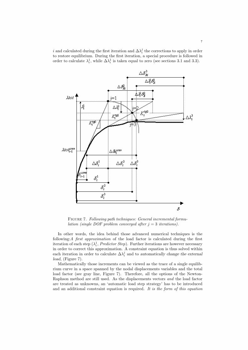
i and calculated during the first iteration and ∆λji the corrections to apply in order
to restore equilibrium. During the first iteration, a special procedure is followed inorder to calculate λ1
i , while ∆λ1i is taken equal to zero (see sections 3.1 and 3.3).
Figure 7. Following path techniques: General incremental formu-lation (single DOF problem converged after j = 3 iterations).
In other words, the idea behind those advanced numerical techniques is thefollowing:A first approximation of the load factor is calculated during the firstiteration of each step (λ1
i , Predictor Step). Further iterations are however necessaryin order to correct this approximation. A constraint equation is thus solved withineach iteration in order to calculate ∆λj
i and to automatically change the externalload, (Figure 7).
Mathematically those increments can be viewed as the trace of a single equilib-rium curve in a space spanned by the nodal displacements variables and the totalload factor (see gray line, Figure 7). Therefore, all the options of the Newton-Raphson method are still used. As the displacements vectors and the load factorare treated as unknowns, an ‘automatic load step strategy’ has to be introducedand an additional constraint equation is required. It is the form of this equation

8 P. KOTRONIS AND F. COLLIN
which distinguishes the various iterative strategies studied hereafter. The choice ofthe form of the constraint equation is often driven by geometrical considerations(updated normal plane, spherical path... see section 3.4 for more details).
The following presentation is based on the excellent work presented in [16]. Someelements of the presentation have also been inspired from [2]. Iterative cycles withina step i start at j = 1, which corresponds to an increment of the external load. Theequilibrium iterations commence at j = 2. Two distinct strategies are required forthe successful completion of a single load step in an incremental-iterative scheme:
(1) Selection of a suitable external load increment λ1i for the first iterative cycle
(j = 1) using a load incrementation strategy ;(2) Selection of an appropriate iterative strategy for application in subsequent
iterative cycles (j ≥ 2) with the aim of restoring equilibrium as rapidly aspossible.
A general presentation of appropriate iterative and load incrementation strategiescombined with the advantages of a full Newton-Raphson procedure follows:
3.1. Iterative strategy - The first iterative cycle, j = 1 (Predictor step).
A new load step i starts with the computation of the tangent stiffness matrix [Ktg]0
i
based on the known displacements and stresses at the conclusion of the previousstep. The ‘tangent’ displacements {δI}
1
i for this load step are then computed asthe solution of
(3.3)[
Ktg]0
i{δI}
1
i = {FI} ,
The magnitude of the displacements is arbitrary only their direction is impor-tant. Next the value of the initial load increment λ1
i is determined according to aparticular load incrementation strategy described in section 3.3. The incrementaldisplacements are then evaluated by scaling the tangent displacements
(3.4) {∆δ}1
i = λ1
i {δI}1
i ,
and the total displacements and total load level are updated from those at theconclusion of the previous load step as follows (∆λ1
i is considered equal to zero):
(3.5) {δ}1
i = {δ}conv
i−1+ {∆δ}
1
i ,
(3.6) λtot1i = λtotconvi−1 + λ1
i ,
At this stage the solution invariably does not satisfy total equilibrium and so addi-tional iterative cycles are required to restore equilibrium.
3.2. Iterative strategy - Equilibrium iterative cycles, j ≥ 2. The incrementalchange in the displacements can be written as the solution of
(3.7)[
Ktg]j−1
i{∆δ}
j
i = λtotji {FI} − {Fint}j−1
i ,
or using equation (3.2)
9
(3.8)[
Ktg]j−1
i{∆δ}
j
i = ∆λji {FI} − {ψ}
j−1
i ,
(3.9) {ψ}j−1
i = {Fint}j−1
i − (λtotconvi−1 + λ1
i +
j∑
j=2
∆λj−1
i ) {FI} ,
In the above expression {ψ}j−1
i represents the internal out-of-balance (‘residual’)
force acting on the structure. [Ktg]j−1
i is calculated at {δ}j−1
i , the accumulatedincremental displacement vector of the step i from iteration 1 to j−1. The internal
force vector {Fint}j−1
i is computed as usual with the Finite Element Method byintegrating the generalized stress resultants through the volume of each elementand then summing the elemental contributions [5].
The right-hand side of the equation (3.8) is linear in ∆λji and so the final solution
can be written as the linear combination of two vectors:
(3.10) {∆δ}j
i = ∆λji {δI}
j
i + {∆δR}j
i ,
{δI}j
i are the displacements computed as follows:
(3.11)[
Ktg]j−1
i{δI}
j
i = {FI} ,
{∆δR}j
i are the displacements obtained as the solution of
(3.12)[
Ktg]j−1
i{∆δR}
j
i = −{ψ}j−1
i ,
using a conventional Full Newton-Raphson procedure. The total load level iscalculated according to eq.(3.2) and the total displacements as follows:
(3.13) {δ}j
i = {δ}j−1
i + {∆δ}j
i ,
The variation of the load parameter ∆λji is obtained by solving an appropriate
constraint equation as described in section 3.4. Iterative cycles are continued untila convergence criterion based on the forces and/or the displacements is satisfied.If convergence in not achieved within a number of iterations specified by the user,or if divergence of the solution is detected, the solution for this load step shouldrecommence with the application of a reduced initial load increment.
3.3. Load incrementation strategy. When commencing a load step i an initialload increment λ1
i must be chosen. The choice of the increment size is importantand should reflect the current degree of non-linearity. If the initial load incrementis too large then convergence will be slow or may not occur at all or we take therisk to miss certain ‘unstable paths’ of the nonlinear behavior of the structure (thesolution would for example ‘jump’ from point L to point L’, Figure 6). If the initialload increment is too small then more converged states are computed than arestrictly necessary [20].
The automatically chosen load increment must also be of the correct sign, ne-cessitating measures capable of detecting when maximum and minimum points on
10 P. KOTRONIS AND F. COLLIN
the load-deflection curve have been passed. If the uncorrect sign is chosen solution‘doubles back’ or oscillates and subsequently fails to converge [20].
Choosing the increment size: Two classes of methods are often used toproper adapt the load factor from one increment to another. The first class isbased on the direct adaption of the load increment [17],[20],[35] and the second oneon the evolution of the current stiffness parameter defined in [8],[9],[10].
The direct adaption of load increment uses the ratio of the actual number ofiterations required for convergence in the previous load step Jd−1, a user-defineddesired number of iterations for convergence Jd and an exponent γ
(3.14) X1
i = ±X1
i−1(Jd
Jd−1
)γ ,
X can be either λ1i or the arc-length l (see eq.(4.2)). The value of the exponent
γ lies typically between 0.25 and 1 [7],[17],[18],[20],[35]. The desired number ofiterations is usually set equal to 3 [20], 5 or 6 [25].
Following the second method, the initial load increment is calculated accordingto an unscaled version of the current stiffness parameter as explained in [16]:
(3.15) SX,i =
[
{δI}1
1
]T
{FI}[
{δI}1
i
]T
{FI}
,
In the previous expression T states for the transpose of a vector. SX,i has theinitial value of unity for any non-linear system. Values of SX,i less than and greaterthan unity indicate ‘softening’ and ‘stiffening’ systems respectively. The expressionfor automatic load incrementation takes then the following form:
(3.16) X1
i = ±X1
i−1
∣
∣
∣
∣
∆SX
∆SX,i.
∣
∣
∣
∣
,
in which ∆SX is a prescribed scalar constant which may either be entered asinput to the program, or calculated using the values of the current stiffness para-meters calculated for the first two load steps, i.e. ∆SX = SX,2 − SX,1 and ∆SX,i
is the change in the current stiffness parameter from the previous load step to thecurrent load step i.e ∆SX,i = SX,i − SX,i−1.
In regions of the load-displacement response which are nearly linear ∆SX,i maybe small, in which case equation (3.16) will lead to large initial load increments X1
i .For this reason it is desirable to specify a maximum absolute value for the initialload increment calculated by eq.(3.16), [16].
Chan [14] uses the following simpler application of the current stiffness parameterfor automatic load incrementation
(3.17) X1
i = ±X1
1 | SX,i|η,
in which the exponent η usually equals 1. In regions of displacement limit pointsSX may become larger (greater than one) and so it is desirable to specify a maxi-mum value of |SX | to limit the load step size.
11
Choosing the sign of the increment: The proper sign of the new load fac-tor increment λ1
i should follow that of the previous increment unless the determinantof the stiffness matrix at the beginning of the new increment changes sign. One hasto store the sign of the determinant of the stiffness matrix at the end of each stepand to look the existence of a negative pivot in the triangularization of the globalstiffness matrix at the beginning of the new increment. This is an indicator thatthe determinant of the tangent stiffness matrix changes sign [17],[20],[35] and thata critical point has been overcome. In relation to the adopted solution procedure,
this will occur when one of the terms in [D], the diagonal matrix of the [L] [D] [L]T
factorisation of [Ktg]1
i is negative (which implies one negative eigenvalue for thestiffness matrix).
Remark:
• The determinant criterion does not work properly when multiple negativeeigenvalues exist (i.e., in the presence of bifurcation points). In that case,the code will oscillate about this bifurcation point. It is recommendedthen, until more advanced path-following techniques are available to stopthe code and with the aid of ‘restarts’ and manual intervention to try tounderstand what is happening [20].
Another criterion was proposed by Bergan [8] who suggested that a change inthe sign should occur upon reversal of the sign of the incremental work ∆W :
(3.18) ∆W = λ1
i {δI}1
i {FI}
According to [25], if all increments would be infinitely small and if no bifurcationpoints are present on the loading path, the incremental work criterion coincides with
the appearance of a negative determinant of [Ktg]1
i . In [16] however, it is mentionedthat the external work sign is deficient in the vicinity of displacement limit points,while the determinant criterion is not. On the basis of the two previous criteria, thefollowing proposal to determine the proper sign of the load estimator is proposedin [7].
(3.19) λ1
i = +∣
∣λ1
i
∣
∣ if {∆δa}conv
i−1{δI}
1
i ≥ 0
(3.20) λ1
i = −∣
∣λ1
i
∣
∣ if {∆δa}conv
i−1{δI}
1
i < 0
{∆δa}conv
i−1is the accumulated converged incremental displacement vector of the
previous step (Figure 7). The effectiveness of the criterion was confirmed in [38].However, criteria based on the sign of the incremental work seem to be insensitive(do not respond) to bifurcation according to [20]...
3.4. Constraint equations for calculating ∆λji . The iterative change ∆λj
i isregarded as an additional unknown variable. In order to calculate it, various con-straint equations are proposed by different workers. Some of them are summarizedbelow:
• If ∆λji is held equal to 0 at every iteration one obtains the classical Full
Newton-Raphson method (with load control). As mentioned in section
12 P. KOTRONIS AND F. COLLIN
2.2, this iterative strategy does not permit to pass load limit points (dis-placement limit points) if a force (displacement) compound is used as thecontrolling parameter.
• Chan [14] proposed the following equation defined as the ‘minimum residualdisplacement’ method:
(3.21) ∆λji =
−[
{δI}j
i
]T
{∆δR}j
i
[
{δI}j
i
]T
{δI}j
i
,
This method guarantees a minimum value for the unbalanced displacementnorm in each iteration.
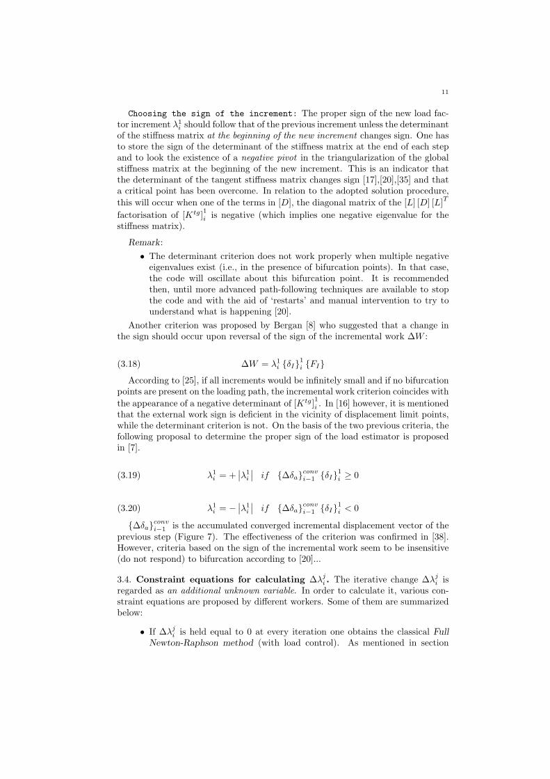
• The ‘updated normal plane method’, where the iterative path follows a‘plane’ normal to the tangent vector {t} of Figure 8, [35]:
(3.22) ∆λji =
−[
{∆δa}j−1
i
]T
{∆δR}j
i
[
{∆δa}j−1
i
]T
{δI}j
i
,
with {∆δa}j−1
i the accumulated incremental displacement vector of the stepi from iteration 1 to j − 1.
Figure 8. The updated normal plane method (single DOF problem).
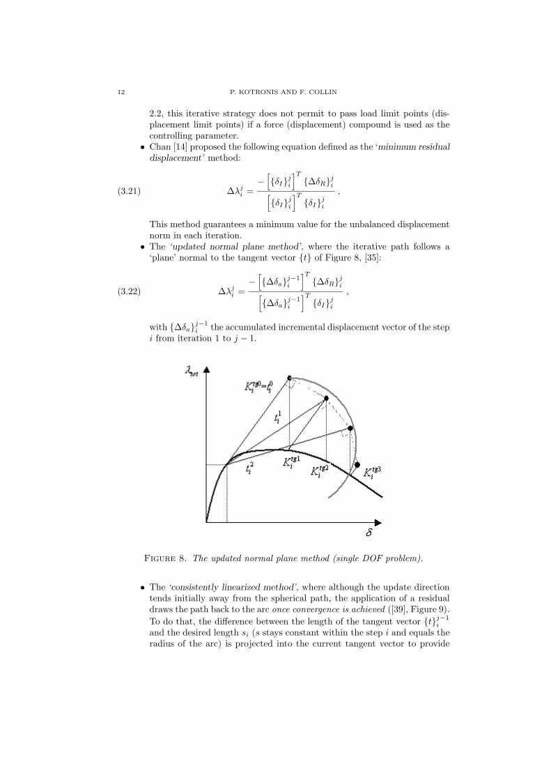
• The ‘consistently linearized method’, where although the update directiontends initially away from the spherical path, the application of a residualdraws the path back to the arc once convergence is achieved ([39], Figure 9).
To do that, the difference between the length of the tangent vector {t}j−1
i
and the desired length si (s stays constant within the step i and equals theradius of the arc) is projected into the current tangent vector to provide
13
the residual for the orthogonality expression (for more details see [24]) :
(3.23) ∆λji =
−∥
∥
∥{t}
j−1
i
∥
∥
∥(∥
∥
∥{t}
j−1
i
∥
∥
∥− si) −
[
{∆δa}j−1
i
]T
{∆δR}j
i
[
{∆δa}j−1
i
]T
{δI}j
i
,
Figure 9. The consistently linearized method (single DOF problem).
• The ‘explicit iteration on spheres’ requires the formulation of a residualbased on the error that would be obtained using an orthogonal iterationpath. This error can be corrected in advance to provide the desired arc.Contrary to the ‘consistently linearized method’ where the path is finallydrown back to the arc only at the end of the step (once convergence isachieved), now the path is drown back to the arc at the end of each iteration.The following algorithm is proposed in [24], (Figure 10):
(1) Calculate the update for orthogonal iteration
(3.24) ∆λji =
−[
{∆δa}j−1
i
]T
{∆δR}j
i
[
{∆δa}j−1
i
]T
{δI}j
i
,
(2) Calculate the associate displacement vector
(3.25) {∆δ}j
i = ∆λji {δI}
j
i + {∆δR}j
i ,
(3) Find the length of the tangent in the potential configuration
(3.26) tji =
√
∥
∥
∥{t}
j−1
i
∥
∥
∥
2
+[
{∆δ}j
i
]T
{∆δ}j
i ,
(4) Calculate the required residual Rji for explicit iteration on a sphere
(3.27) Rji = −
s2i∥
∥
∥{t}
j−1
i
∥
∥
∥
(∥
∥
∥{t}
j−1
i
∥
∥
∥− si) ,
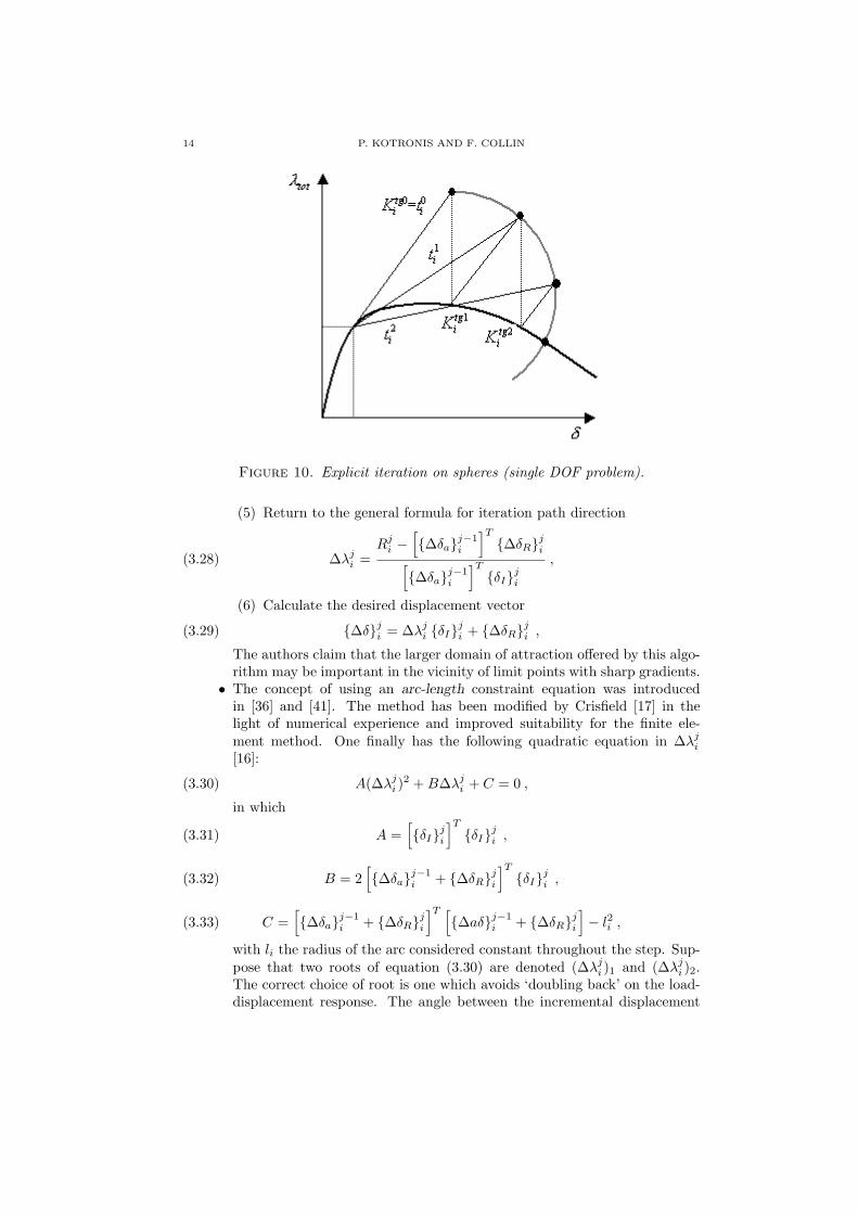
14 P. KOTRONIS AND F. COLLIN
Figure 10. Explicit iteration on spheres (single DOF problem).
(5) Return to the general formula for iteration path direction
(3.28) ∆λji =
Rji −
[
{∆δa}j−1
i
]T
{∆δR}j
i
[
{∆δa}j−1
i
]T
{δI}j
i
,
(6) Calculate the desired displacement vector
(3.29) {∆δ}j
i = ∆λji {δI}
j
i + {∆δR}j
i ,
The authors claim that the larger domain of attraction offered by this algo-rithm may be important in the vicinity of limit points with sharp gradients.
• The concept of using an arc-length constraint equation was introducedin [36] and [41]. The method has been modified by Crisfield [17] in thelight of numerical experience and improved suitability for the finite ele-ment method. One finally has the following quadratic equation in ∆λj
i
[16]:
(3.30) A(∆λji )
2 +B∆λji + C = 0 ,
in which
(3.31) A =[
{δI}j
i
]T
{δI}j
i ,
(3.32) B = 2[
{∆δa}j−1
i + {∆δR}j
i
]T
{δI}j
i ,
(3.33) C =[
{∆δa}j−1
i + {∆δR}j
i
]T [
{∆aδ}j−1
i + {∆δR}j
i
]
− l2i ,
with li the radius of the arc considered constant throughout the step. Sup-pose that two roots of equation (3.30) are denoted (∆λj
i )1 and (∆λji )2.
The correct choice of root is one which avoids ‘doubling back’ on the load-displacement response. The angle between the incremental displacement
15
vector before the present iteration and the incremental displacement vectorafter the current iteration should be positive. For the two possible roots,the corresponding angles are defined in [16],[17] as:
(3.34) θ1,2 =[
{∆δa}j−1
i + (∆λji )1,2 {δI}
j
i + {∆δR}j
i
]T
{∆δa}j−1
i ,
The correct choice of root ∆λji is the one which gives the minimum positive
angle θ, [21].The quadratic equation (3.30) possess imaginary roots if B2−4AC is less
than zero. This situation can arise if the initial load increment is too largeand the structure exhibits multiple instability directions at a point. For thiscase it is preferred that the finite element code writes a warning messageand recommences the solution for this load step with the application of areduced initial load increment.
Remarks:
• For graphical purposes, the stiffness matrix in Figure 8 to Figure 10 staysconstant within the iterations. However, the equations (3.21) to (3.34) arepresented in their general form.
• At the beginning of the section 3.1 it is mentioned that the calculation of
the tangent stiffness matrix [Ktg]0
i is based on the known displacementsand stresses at the conclusion of the previous step. However, in order totake a better guess for starting the incremental-iterative scheme within astep some finite element codes usually extrapolate the DOF solution usingthe previous history (i.e., in LAGAMINE the velocities of the step i areconsidered equal to the converged velocities of the step i− 1, see also [2]).
• A general formulation based on orthogonality principles able to derive mostof the previous constraint equations, to illustrate their relationships and toprovide a geometrical explication is proposed in [24].
• A careful analysis of the incremental/iterative behavior using equation 3.30showed severe numerical difficulties in the presence of very sharp snap-backs(particularly those occurring in fracture mechanics or damage mechanicsboth for failure initiation and crack propagation [21]). The problems wereassociated with an ‘incorrect choice of root’ from the two solutions to thequadratic equation in the load level change. The idea behind the choiceof minimum angle is to avoid the solution ‘doubling back’. However, for avery sharp snap-back , one wants the solution to double back. Hellweg andCriesfild proposed to select the root with the minimum residual [21],[28].This new criterion can easily be added to an existing arc-length methodby including one additional loop over the number of the roots. Naturally,this approach is more expensive than the conventional one. In addition,for most relatively smooth problems, this technique is not needed. Criesfild[21] propose to turn on this option when the code exhibits convergencedifficulties or the analyst anticipates the existence of snap-backs. A morerecent paper however [30], showed that even this new criterion may proveinsufficient.
• The ‘explicit iteration on spheres’ provides exactly the same results as theconcept of the arc-length constraint equation [17] without the solution ofa quadratic equation and the selection of one root [24]. However, this
16 P. KOTRONIS AND F. COLLIN
approach requires a solution for the intersection of the tangent with theupdated normal plane. In the case of sharp turns on the loading path thisintersection may still yield poor results [25].
• An additional scalar parameter β is often found in the literature in theexpressions of the different constraint equations. It is a scaling factor whichdeals with the dimensional incompatibility between the degrees of freedomand the load factor λtotji (this inconsistency appears only if different typesof degree of freedoms are present). Setting β equal to zero (which is thecase for the equations presented in this work) results in constraint equationsthat are explicitly written in the hyperspace of the DOF only. Although itis known that β = 0 is often the recommended choice, general conclusionscannot be drown and the best choice of β is in fact structure dependent[25]. With β equal to zero the quadratic equation proposed by Crisfield[17] corresponds to the cylindrical arc-length method, while a non-zero βcorresponds to the spherical arc-length method.
• Geometrically non-linear problem are mainly solved by techniques whichinvolve the control of all DOF. Physically non-linear problems often re-quire the control of a limited number of degrees of freedom, due to local-ized deformations [20],[22],[25],[30],[31],[42], [43]. Localization problems arecharacterized by the fact that local DOF dominate the overall mechanicalbehavior of the considered discretized medium. Using all DOF’s may resultsin an unstable Newton-Raphson scheme [25].
4. Algorithm used for the implementation of path following
techniques into LAGAMINE
The principal subroutines that have been changed in order to implement theprevious following path techniques into the finite element code LAGAMINE are:SOLSYS.F, ARCLEN.F, LAMIN2.F, LICHAB.F, INIDDL.F, NORME1.F, AU-TOMA.F, AUTOMU.F, AUTORD.F, ASSEL.F, CLCOQ4.F... The direct adaptionof load increment is used to choose the increment size (jstep=-3. However, consider-ing jstep=-1 one uses the FACMU variable as it is usually the case in LAGAMINE).The sign of the load increment is determined according to the sign of the determi-nant of the tangent stiffness matrix. The algorithm takes the following form:
Step i = 1
• The ‘classical strategy’ already implemented into LAGAMINE is used. Theuser defines an initial loading (force or displacement) and the code proceedsto the resolution with the Full Newton-Raphson procedure. In that wayone can take advantage of all the functionalities already presented in thecode (define a maximum number of iterations needed for convergence, amaximum and a minimum value step, a multiplicator for the load step -if one does not want to use the direct adaption of the load increment -, atermination load factor etc. The relative norms of both residual forces anddisplacements are adopted as criteria for convergence.
• During this first step the code calculates the reference external load fac-tor {FI} that stays constant throughout the whole loading (proportionalloading, eq.(2.6)).
17
• Reading the desired number of iterations for convergence Jd and the expo-nent γ. Those parameters are used for the direct adaption of load incrementmethod, eq.(3.14).
Step i = 2 - Iteration j = 1
• The starting load factor λ12 is taken equal to load factor (force or dis-
placement) of the converged first step. This starting load factor has to bebetween 20% and 40% of the anticipated maximum load [16].
• Calculate the tangent stiffness matrix [Ktg]0
2.
• Calculate the ‘tangent’ displacements {δI}1
2from eq.(3.3).
• Calculate the incremental displacements {∆δ}1
2by scaling the ‘tangent’
displacements, eq.(3.4).
• Update the total displacements {δ}1
2= {∆δ}
1
2
• Update the total load factor λtot12 = λ12
• Calculate the initial radius (positive value) using the following equation[16]:
(4.1) (l1)2 = (∆λ1
2)2
[
{δI}1
2
]T
{δI}1
2,
Step i > 2 - Iteration j = 1
• Read the ratio of the actual number of iterations required for convergencein the previous load step Jd−1. Update the radius l as follows:
(4.2) li = li−1(Jd
Jd−1
)γ ,
The updated radius stays constant throughout the whole step i.
• Calculate the tangent stiffness matrix [Ktg]0
i (at {δ}conv
i−1, the accumulated
converged displacement vector of the previous step, unless the code ex-trapolates the DOF solution using the previous history - see section 3.4).
Proceed to the factorisation of the stiffness matrix [Ktg]0
i = [L] [D] [L]T,
check the existence of negative pivots and the sign of the determinant ofthe stiffness matrix at convergence of the previous step. Define in that wayif m = +1 or m = −1.
• Calculate λ1i as follows:
(4.3) λ1
i = mli
√
[
{δI}1
i
]T
{δI}1
i
,
• Calculate the ‘tangent’ displacements {δI}1
i from eq.(3.3).
• Calculate the incremental displacements {∆δ}1
i by scaling the ‘tangent’displacements, eq.(3.4).
• Update the total displacements {δ}1
i = {∆δ}1
i
• Update the total load factor λtot1i = λ1i
Step i 6= 1 - Iteration j 6= 1
• Calculate the tangent stiffness matrix [Ktg]j−1
i (at {δ}j−1
i , the accumulateddisplacement vector at step i iteration j − 1).
18 P. KOTRONIS AND F. COLLIN
• Calculate the internal (‘residual’) force vector {Fint}j−1
i acting on the struc-ture as usual with the Finite Element Method by integrating the generalizedstress resultants through the volume of each element and then summing theelemental contributions.
• Calculate the internal out-of-balance (‘residual’) force acting on the struc-ture according to eq.(3.9).
• Calculate {∆δR}j
i using eq.(3.12) and the classical Full Newton-Raphsonmethod.
• Calculate the ‘tangent’ displacements {δI}j
i according to eq.(3.11).
• Calculate ∆λji using one of the constraint equations presented in section
3.4 (equations (3.21) to (3.34)).
• Calculate the incremental displacements {∆δ}j
i from eq.(3.10).
• Update the total displacements {δ}j
i with eq.(3.13).• Update the total load factors according to eq.(3.2).• Test of convergence - Stock the sign of the determinant of the stiffness
matrix. If the number of iterations needed for convergence exceeds themaximum number defined by the user or if divergence of the solution isdetected, the solution for this load step recommence with the applicationof a reduced initial load increment.
Remark:
• One of the disadvantages of the following path techniques is that the termi-nation load factor is not respected (the incrementation of the load factor isautomatic and not user controlled). In order to be sure that the code stopsat the prescribed termination load factor the following procedure is usedin LAGAMINE: The code detects when the total load factor is near thedesired termination load factor and changes automatically to the ‘classicalstrategy’. It imposes then an incremental load factor such as the final stepis done with the desired termination factor. Unfortunately, this option didnot perform correctly in some of the examples presented hereafter.
5. Examples using different following path techniques
The first three examples concern geometrical non-linear problems and the lastone a 1D concrete bar.
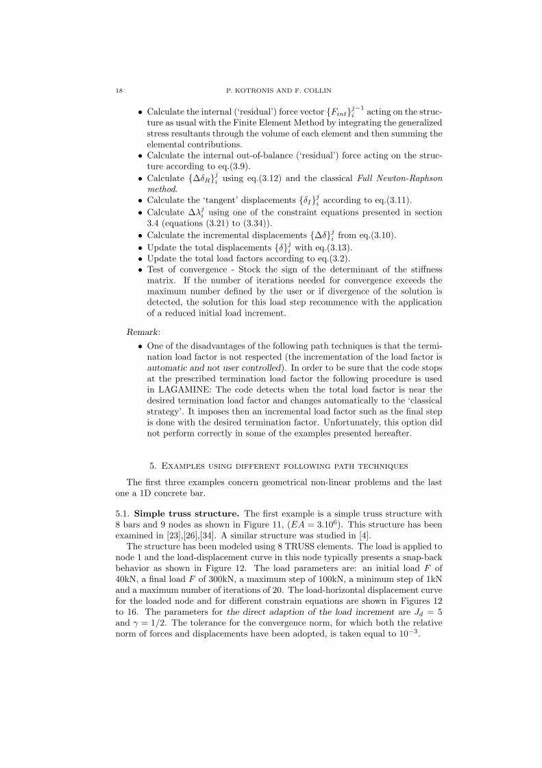
5.1. Simple truss structure. The first example is a simple truss structure with8 bars and 9 nodes as shown in Figure 11, (EA = 3.106). This structure has beenexamined in [23],[26],[34]. A similar structure was studied in [4].
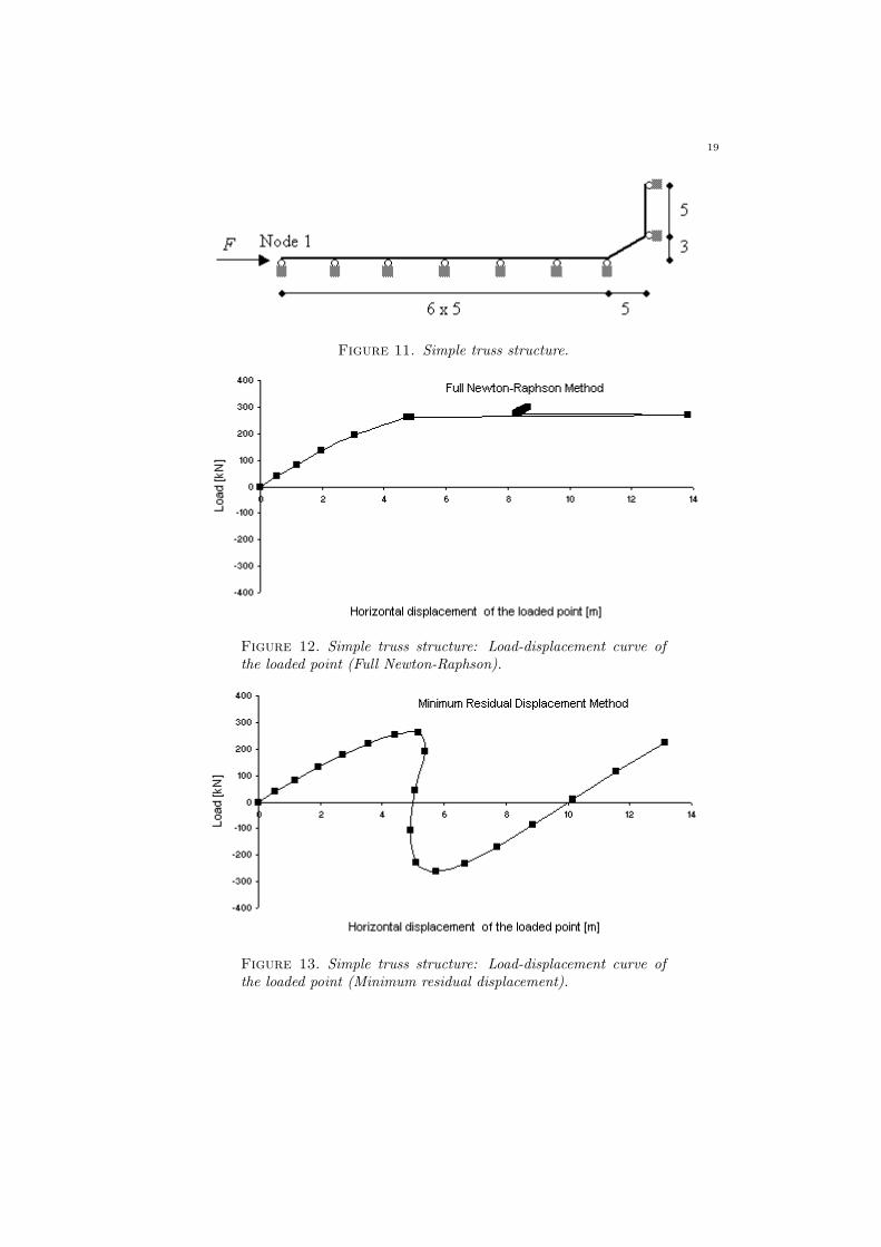
The structure has been modeled using 8 TRUSS elements. The load is applied tonode 1 and the load-displacement curve in this node typically presents a snap-backbehavior as shown in Figure 12. The load parameters are: an initial load F of40kN, a final load F of 300kN, a maximum step of 100kN, a minimum step of 1kNand a maximum number of iterations of 20. The load-horizontal displacement curvefor the loaded node and for different constrain equations are shown in Figures 12to 16. The parameters for the direct adaption of the load increment are Jd = 5and γ = 1/2. The tolerance for the convergence norm, for which both the relativenorm of forces and displacements have been adopted, is taken equal to 10−3.
19
Figure 11. Simple truss structure.
Figure 12. Simple truss structure: Load-displacement curve ofthe loaded point (Full Newton-Raphson).
Figure 13. Simple truss structure: Load-displacement curve ofthe loaded point (Minimum residual displacement).
20 P. KOTRONIS AND F. COLLIN
Figure 14. Simple truss structure: Load-displacement curve ofthe loaded point (Updated normal plane).
Figure 15. Simple truss structure: Load-displacement curve ofthe loaded point (Explicit iteration on spheres).
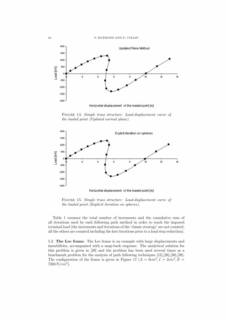
Table 1 resumes the total number of increments and the cumulative sum ofall iterations used by each following path method in order to reach the imposedterminal load (the increments and iterations of the ‘classic strategy’ are not counted,all the others are counted including the lost iterations prior to a load step reduction).
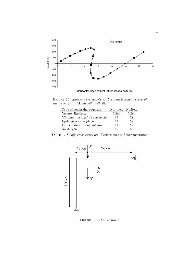
5.2. The Lee frame. The Lee frame is an example with large displacements andinstabilities, accompanied with a snap-back response. The analytical solution forthis problem is given in [29] and the problem has been used several times as abenchmark problem for the analysis of path following techniques [15],[26],[38],[39].The configuration of the frame is given in Figure 17 (A = 6cm2, I = 2cm4, E =720kN/cm2).
21
Figure 16. Simple truss structure: Load-displacement curve ofthe loaded point (Arc-length method).
Type of constraint equation No. incr. No.iter.Newton-Raphson failed failedMinimum residual displacement 17 58Updated normal plane 17 58Explicit iteration on spheres 17 58Arc-length 19 68
Table 1. Simple truss structure - Performance and incrementation.
Figure 17. The Lee frame.
22 P. KOTRONIS AND F. COLLIN
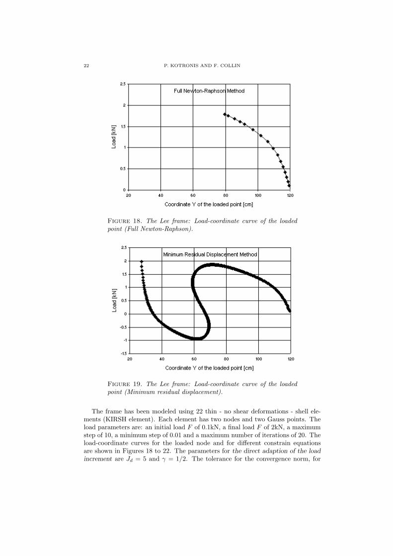
Figure 18. The Lee frame: Load-coordinate curve of the loadedpoint (Full Newton-Raphson).
Figure 19. The Lee frame: Load-coordinate curve of the loadedpoint (Minimum residual displacement).
The frame has been modeled using 22 thin - no shear deformations - shell ele-ments (KIRSH element). Each element has two nodes and two Gauss points. Theload parameters are: an initial load F of 0.1kN, a final load F of 2kN, a maximumstep of 10, a minimum step of 0.01 and a maximum number of iterations of 20. Theload-coordinate curves for the loaded node and for different constrain equationsare shown in Figures 18 to 22. The parameters for the direct adaption of the loadincrement are Jd = 5 and γ = 1/2. The tolerance for the convergence norm, for
23
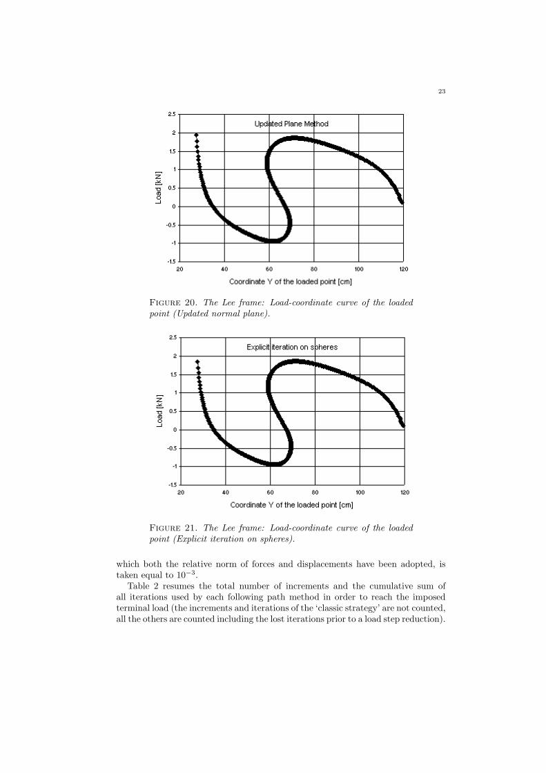
Figure 20. The Lee frame: Load-coordinate curve of the loadedpoint (Updated normal plane).
Figure 21. The Lee frame: Load-coordinate curve of the loadedpoint (Explicit iteration on spheres).
which both the relative norm of forces and displacements have been adopted, istaken equal to 10−3.
Table 2 resumes the total number of increments and the cumulative sum ofall iterations used by each following path method in order to reach the imposedterminal load (the increments and iterations of the ‘classic strategy’ are not counted,all the others are counted including the lost iterations prior to a load step reduction).
24 P. KOTRONIS AND F. COLLIN
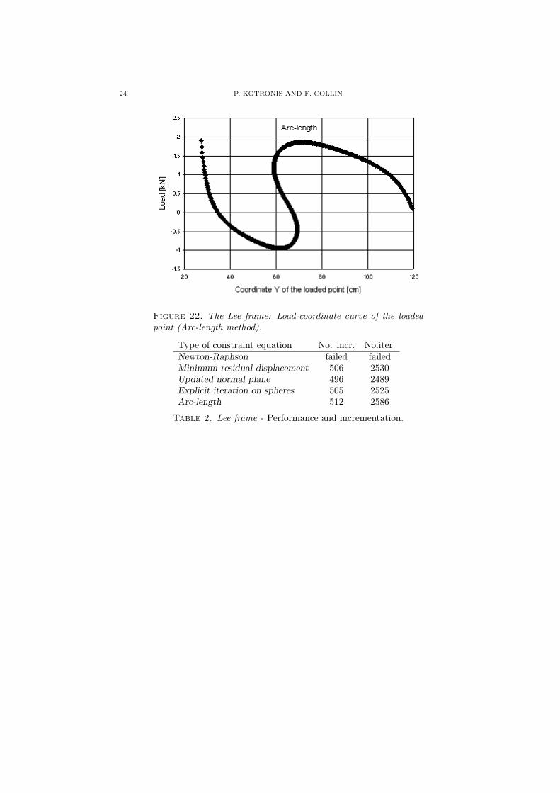
Figure 22. The Lee frame: Load-coordinate curve of the loadedpoint (Arc-length method).
Type of constraint equation No. incr. No.iter.Newton-Raphson failed failedMinimum residual displacement 506 2530Updated normal plane 496 2489Explicit iteration on spheres 505 2525Arc-length 512 2586
Table 2. Lee frame - Performance and incrementation.
25
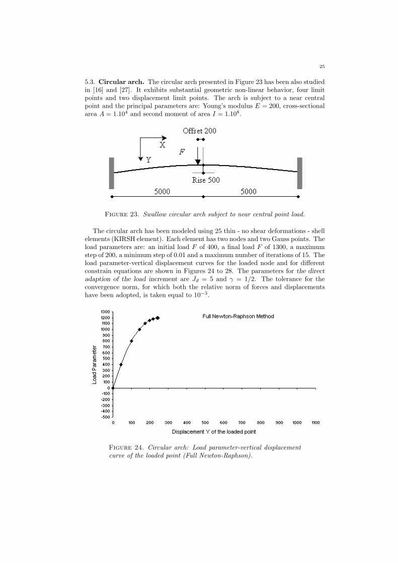
5.3. Circular arch. The circular arch presented in Figure 23 has been also studiedin [16] and [27]. It exhibits substantial geometric non-linear behavior, four limitpoints and two displacement limit points. The arch is subject to a near centralpoint and the principal parameters are: Young’s modulus E = 200, cross-sectionalarea A = 1.104 and second moment of area I = 1.108.
Figure 23. Swallow circular arch subject to near central point load.
The circular arch has been modeled using 25 thin - no shear deformations - shellelements (KIRSH element). Each element has two nodes and two Gauss points. Theload parameters are: an initial load F of 400, a final load F of 1300, a maximumstep of 200, a minimum step of 0.01 and a maximum number of iterations of 15. Theload parameter-vertical displacement curves for the loaded node and for differentconstrain equations are shown in Figures 24 to 28. The parameters for the directadaption of the load increment are Jd = 5 and γ = 1/2. The tolerance for theconvergence norm, for which both the relative norm of forces and displacementshave been adopted, is taken equal to 10−3.
Figure 24. Circular arch: Load parameter-vertical displacementcurve of the loaded point (Full Newton-Raphson).
26 P. KOTRONIS AND F. COLLIN
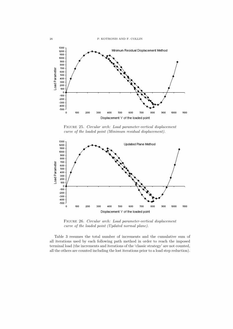
Figure 25. Circular arch: Load parameter-vertical displacementcurve of the loaded point (Minimum residual displacement).
Figure 26. Circular arch: Load parameter-vertical displacementcurve of the loaded point (Updated normal plane).
Table 3 resumes the total number of increments and the cumulative sum ofall iterations used by each following path method in order to reach the imposedterminal load (the increments and iterations of the ‘classic strategy’ are not counted,all the others are counted including the lost iterations prior to a load step reduction).
27
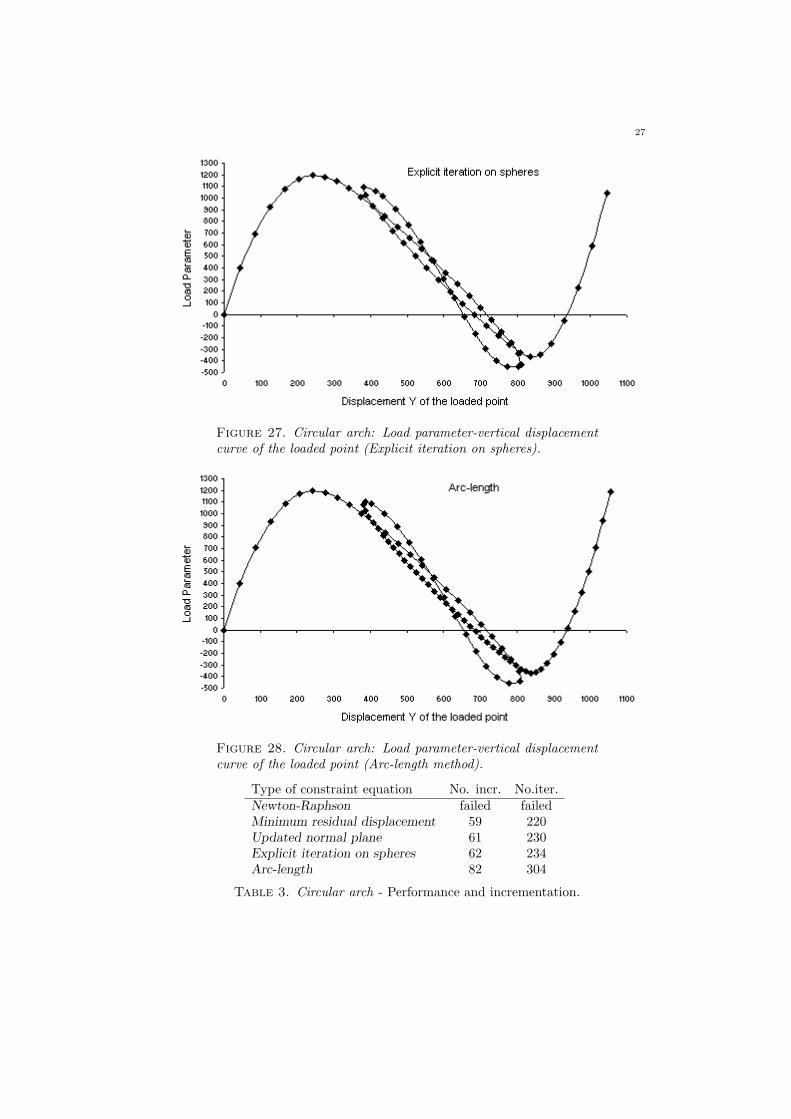
Figure 27. Circular arch: Load parameter-vertical displacementcurve of the loaded point (Explicit iteration on spheres).
Figure 28. Circular arch: Load parameter-vertical displacementcurve of the loaded point (Arc-length method).
Type of constraint equation No. incr. No.iter.Newton-Raphson failed failedMinimum residual displacement 59 220Updated normal plane 61 230Explicit iteration on spheres 62 234Arc-length 82 304
Table 3. Circular arch - Performance and incrementation.
28 P. KOTRONIS AND F. COLLIN
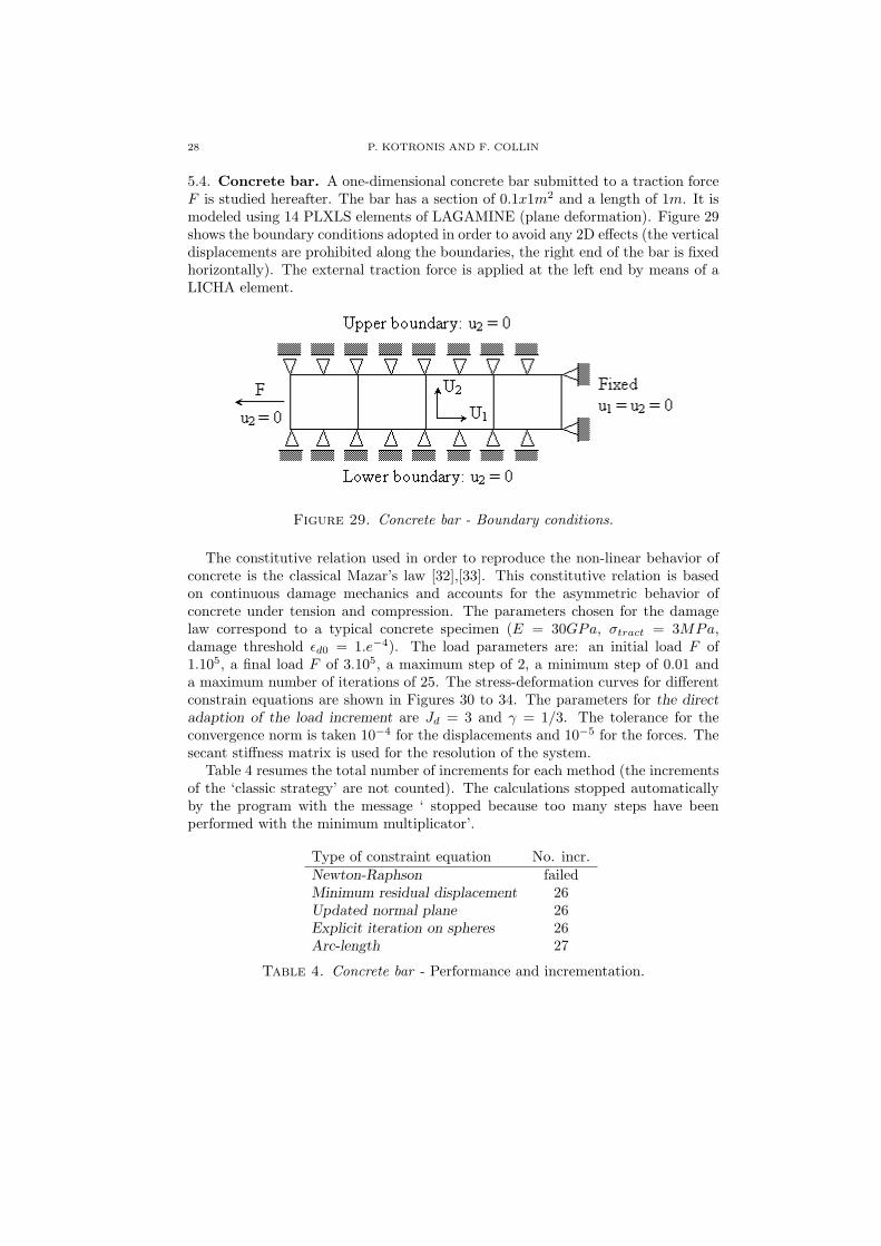
5.4. Concrete bar. A one-dimensional concrete bar submitted to a traction forceF is studied hereafter. The bar has a section of 0.1x1m2 and a length of 1m. It ismodeled using 14 PLXLS elements of LAGAMINE (plane deformation). Figure 29shows the boundary conditions adopted in order to avoid any 2D effects (the verticaldisplacements are prohibited along the boundaries, the right end of the bar is fixedhorizontally). The external traction force is applied at the left end by means of aLICHA element.
Figure 29. Concrete bar - Boundary conditions.
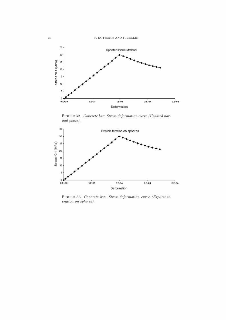
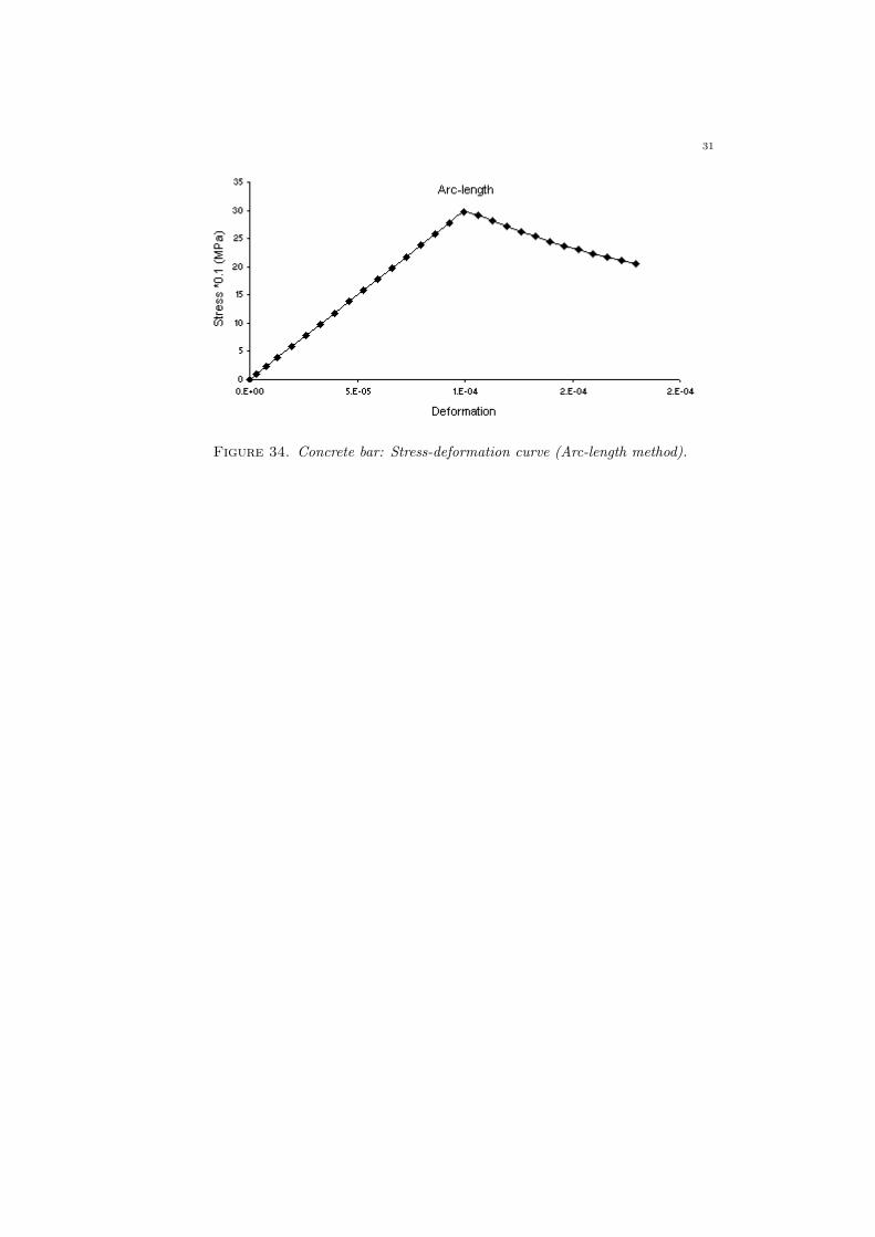
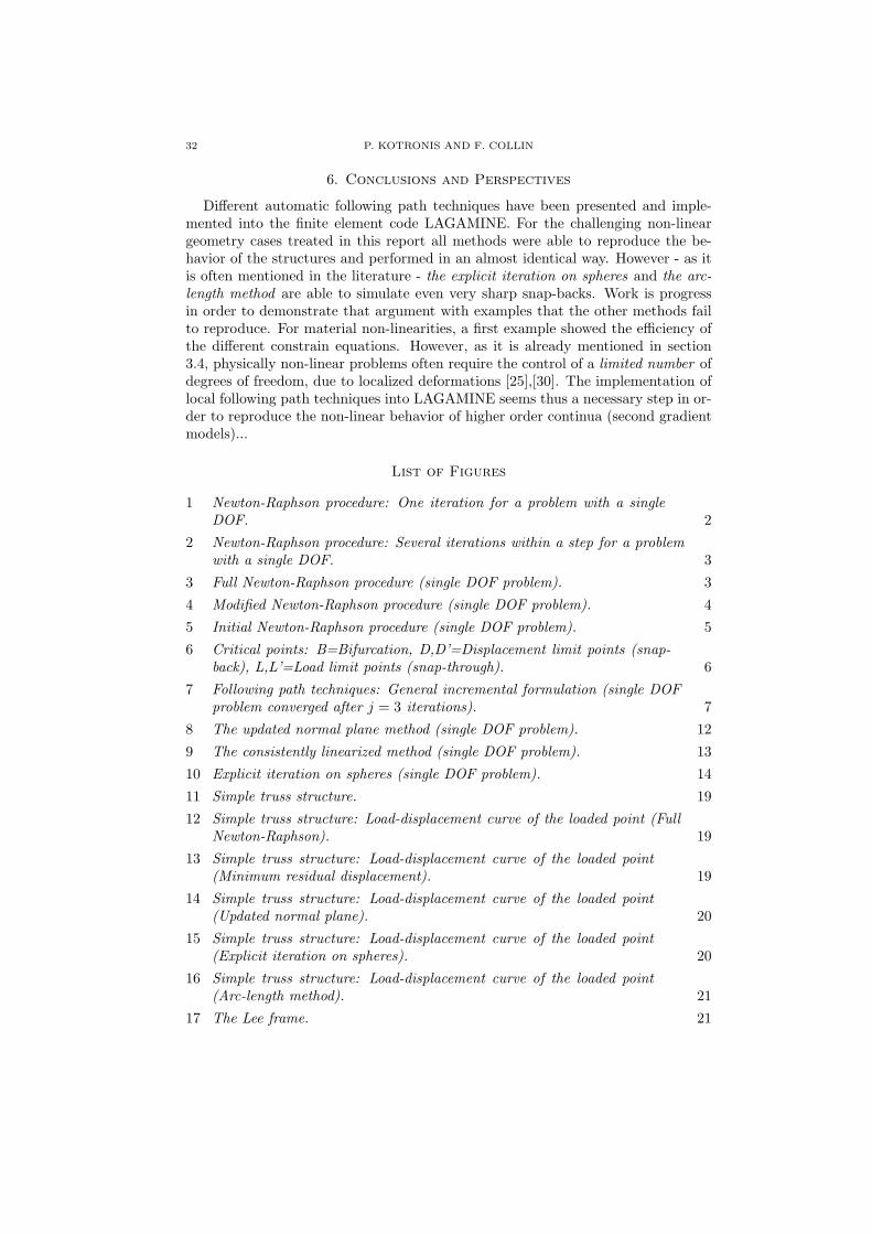
The constitutive relation used in order to reproduce the non-linear behavior ofconcrete is the classical Mazar’s law [32],[33]. This constitutive relation is basedon continuous damage mechanics and accounts for the asymmetric behavior ofconcrete under tension and compression. The parameters chosen for the damagelaw correspond to a typical concrete specimen (E = 30GPa, σtract = 3MPa,damage threshold ǫd0 = 1.e−4). The load parameters are: an initial load F of1.105, a final load F of 3.105, a maximum step of 2, a minimum step of 0.01 anda maximum number of iterations of 25. The stress-deformation curves for differentconstrain equations are shown in Figures 30 to 34. The parameters for the directadaption of the load increment are Jd = 3 and γ = 1/3. The tolerance for theconvergence norm is taken 10−4 for the displacements and 10−5 for the forces. Thesecant stiffness matrix is used for the resolution of the system.
Table 4 resumes the total number of increments for each method (the incrementsof the ‘classic strategy’ are not counted). The calculations stopped automaticallyby the program with the message ‘ stopped because too many steps have beenperformed with the minimum multiplicator’.
Type of constraint equation No. incr.Newton-Raphson failedMinimum residual displacement 26Updated normal plane 26Explicit iteration on spheres 26Arc-length 27
Table 4. Concrete bar - Performance and incrementation.
29
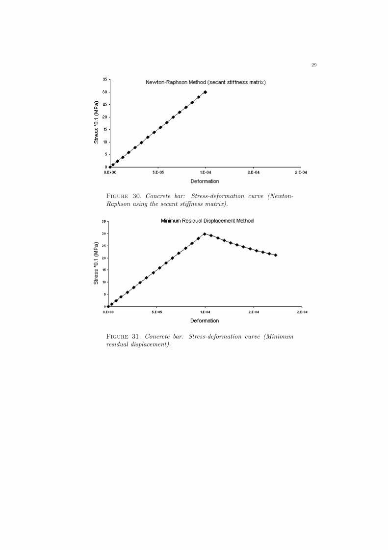
Figure 30. Concrete bar: Stress-deformation curve (Newton-Raphson using the secant stiffness matrix).
Figure 31. Concrete bar: Stress-deformation curve (Minimumresidual displacement).
30 P. KOTRONIS AND F. COLLIN
Figure 32. Concrete bar: Stress-deformation curve (Updated nor-mal plane).
Figure 33. Concrete bar: Stress-deformation curve (Explicit it-eration on spheres).
31
Figure 34. Concrete bar: Stress-deformation curve (Arc-length method).
32 P. KOTRONIS AND F. COLLIN
6. Conclusions and Perspectives
Different automatic following path techniques have been presented and imple-mented into the finite element code LAGAMINE. For the challenging non-lineargeometry cases treated in this report all methods were able to reproduce the be-havior of the structures and performed in an almost identical way. However - as itis often mentioned in the literature - the explicit iteration on spheres and the arc-length method are able to simulate even very sharp snap-backs. Work is progressin order to demonstrate that argument with examples that the other methods failto reproduce. For material non-linearities, a first example showed the efficiency ofthe different constrain equations. However, as it is already mentioned in section3.4, physically non-linear problems often require the control of a limited number ofdegrees of freedom, due to localized deformations [25],[30]. The implementation oflocal following path techniques into LAGAMINE seems thus a necessary step in or-der to reproduce the non-linear behavior of higher order continua (second gradientmodels)...
List of Figures
1 Newton-Raphson procedure: One iteration for a problem with a singleDOF. 2
2 Newton-Raphson procedure: Several iterations within a step for a problemwith a single DOF. 3
3 Full Newton-Raphson procedure (single DOF problem). 3
4 Modified Newton-Raphson procedure (single DOF problem). 4
5 Initial Newton-Raphson procedure (single DOF problem). 5
6 Critical points: B=Bifurcation, D,D’=Displacement limit points (snap-back), L,L’=Load limit points (snap-through). 6
7 Following path techniques: General incremental formulation (single DOFproblem converged after j = 3 iterations). 7
8 The updated normal plane method (single DOF problem). 12
9 The consistently linearized method (single DOF problem). 13
10 Explicit iteration on spheres (single DOF problem). 14
11 Simple truss structure. 19
12 Simple truss structure: Load-displacement curve of the loaded point (FullNewton-Raphson). 19
13 Simple truss structure: Load-displacement curve of the loaded point(Minimum residual displacement). 19
14 Simple truss structure: Load-displacement curve of the loaded point(Updated normal plane). 20
15 Simple truss structure: Load-displacement curve of the loaded point(Explicit iteration on spheres). 20
16 Simple truss structure: Load-displacement curve of the loaded point(Arc-length method). 21
17 The Lee frame. 21
33
18 The Lee frame: Load-coordinate curve of the loaded point (Full Newton-Raphson). 22
19 The Lee frame: Load-coordinate curve of the loaded point (Minimumresidual displacement). 22
20 The Lee frame: Load-coordinate curve of the loaded point (Updated normalplane). 23
21 The Lee frame: Load-coordinate curve of the loaded point (Explicit iterationon spheres). 23
22 The Lee frame: Load-coordinate curve of the loaded point (Arc-lengthmethod). 24
23 Swallow circular arch subject to near central point load. 25
24 Circular arch: Load parameter-vertical displacement curve of the loadedpoint (Full Newton-Raphson). 25
25 Circular arch: Load parameter-vertical displacement curve of the loadedpoint (Minimum residual displacement). 26
26 Circular arch: Load parameter-vertical displacement curve of the loadedpoint (Updated normal plane). 26
27 Circular arch: Load parameter-vertical displacement curve of the loadedpoint (Explicit iteration on spheres). 27
28 Circular arch: Load parameter-vertical displacement curve of the loadedpoint (Arc-length method). 27
29 Concrete bar - Boundary conditions. 28
30 Concrete bar: Stress-deformation curve (Newton-Raphson using the secantstiffness matrix). 29
31 Concrete bar: Stress-deformation curve (Minimum residual displacement). 29
32 Concrete bar: Stress-deformation curve (Updated normal plane). 30
33 Concrete bar: Stress-deformation curve (Explicit iteration on spheres). 30
34 Concrete bar: Stress-deformation curve (Arc-length method). 31
List of Tables
1 Simple truss structure - Performance and incrementation. 21
2 Lee frame - Performance and incrementation. 24
3 Circular arch - Performance and incrementation. 27
4 Concrete bar - Performance and incrementation. 28
References
1. G. Alfano and M.A. Crisfield, Finite element interface models for the delamination analy-
sis of laminated composites:mechanical and computational issues, International Journal for
Numerical Methods in Engineering 50 (2001), no. 7, 1701–1736.2. Inc. ANSYS, Ansys 6.1 documentation, Ansys Inc., 2004.3. J.H. Argyris, Continua and discontinua, Proceedings of the 1st Conference on Matrix Methods
in Structural Mechanics (Wright-Patterson A.F.B. OH, ed.), 1965, pp. 11–189.
34 P. KOTRONIS AND F. COLLIN
4. K. Bathe and Dvorkin E.N., On the automatic solution of non-linear finite element equations,Computer and Structures 17 (1983), no. 5/6, 871–879.
5. K.J. Bathe, Finite element procedures in engineering analysis, Prentice Hall, Inc, New Jersey,1996.
6. J.L. Batoz and G. Dhatt, Incremental displacement algorithms for nonlinear problems, Inter-national Journal for Numerical Methods in Engineering 14 (1979), 1262–1267.
7. P.X. Bellini and A. Chulya, An improved automatic incremental algorithm for the efficient
solution of non linear finite element equations, Computer and Structures 26 (1987), no. 1/2,99–110.
8. P.G. Bergan, Solution techniques for non-linear finite element problems, International Journalfor Numerical Methods in Engineering 12 (1978), 1677–1696.
9. , Solution algorithms for nonlinear structural problems, Computer and Structures 12
(1980), 497–509.
10. , Recent advances in non-linear computational mechanics, ch. 2 - Automatedincremental-iterative solution methods in structural mechanics, pp. 41–62, Hinton E. etal.(eds.) Pineridge Press: Swansea, U.K., 1982.
11. C. Bosco and A. Carpinteri, Discontinuous constitutive response of brittle matrix fibrous
composites, Journal of the Mechanics and Physics of Solids 43 (1995), no. 2, 261–274.12. R. Chambon, S. Crochepeyre, and R. Charlier, An algorithm and a method to search bifurca-
tion points in non-linear problems, International Journal for Numerical Methods in Engini-
neering 51 (2001), 315–332.13. R. Chambon and J.C. Moullet, Uniqueness studies in boundary value problems involving some
second gradient models, Comput. Meth. Appl. Mech. Engng. 193 (2004), 2771–2796.14. S.L. Chan, Geometric and material nonlinear analysis of beam-columns and frames using
the minimum residual displacement method, International Journal of Numerical Methods inEngineering 26 (1988), 2657–2669.
15. Z. Chen and H.L. Schreyer, Secant structural solution strategies under element constraint for
incremental damage, Computer Methods in Applied Mechanics and Engineering 90 (1991),869–884.
16. M.J. Clarke and G.J. Hancock, A study of incremental-iterative strategies for non-linear
analyses, International Journal for Numerical Methods in Engineering 29 (1990), 1365–1991.
17. M.A. Crisfield, A fast incremental-iterative solution procedure that handles snap-through,Computers and Structures 13 (1981), no. 1/3, 55–62.
18. , An arc-length method including line searches and accelerations, International Journalfor Numerical Methods in Engineering 19 (1983), 1269–1289.
19. , Snap-through and snap-back response in concrete structures and the dangers of
under-integration, International Journal for Numerical Methods in Engineering 22 (1986),751–767.
20. , Nonlinear finite element analysis of solids and structures, vol i: Essentials, JohnWiley, Chichester, 1991.
21. , Nonlinear finite element analysis of solids and structures, vol ii: Advanced topics,John Wiley, Chichester, 1991.
22. R. De Borst, Computation of post-bifurcation and post-failure of strain-softening solids, Com-puter and Structures 25 (1987), 211–224.
23. P.H. Feenstra and Schellekens J.C.J., Self-adaptive solution algorithm for a constrained
newton-raphson method, Tech. Report Technical Report 25.2-91-2-13, Delft University of Tech-nology, Delft, The Netherlands, 1991.
24. B.W.R. Forde and Stiemer S.F., Improved arc length orthogonality methods for nonlinear
finite element analysis, Computer and Structures 27 (1987), no. 5, 625–630.
25. M.G.D Geers, Enhanced solution control for physically and geometrically non-linear problems.
part i - the subplane approach, International Journal for Numerical Methods in Engineering46 (1999), 177–204.
26. , Enhanced solution control for physically and geometrically non-linear problems. part
ii - comparative performance analysis, International Journal for Numerical Methods in Engi-neering 46 (1999), 205–230.
27. H.B. Harrison, Elastic-post-buckling response of plane frames, Instability and Plastic collapse
of steel structures, Granada (Morris L.J., ed.), 1983, pp. 56–65.
35
28. H.B. Hellweg and M.A. Crisfield, A new arc-length method for handling sharp snap-backs,Computers and Structures 66 (1998), no. 5, 705–709.
29. S. Lee, F.S. Manuel, and E.C. Rossow, Large deflections and stability of elastic frames, Journalof Enginnering Mechanics Division, Proceedings of the American Society of Civil Enginners94 (1968), no. 2, 521–547.
30. E. Lorentz and P. Badel, A new path-following constraint for strain-softening finite elements
simulations, International Journal for Numerical Methods in Engineering 60 (2004), 499–526.31. I.M. May and Y. Duan, A local arc-length procedure for strain softening, Computer and
Structures 64 (1997), no. 1/4, 297–303.
32. J. Mazars, Application de la mecanique de l’endommagement au comportement non lineaire
et a la rupture du beton de structure, Ph.D. thesis, Universite Paris 6, France, 1984, (Thesede doctorat des Sciences).
33. , A description of micro and macroscale damage of concrete structures, Engineering
Fracture Mechanics 25 (1986), no. 5/6, 729–737.34. G. Powell and J. Simons, Improved iteration strategy for nonlinear structures, International
Journal for Numerical Methods in Engineering 17 (1981), 1455–1467.35. E. Ramm, Strategies for tracing the non-linear response near limit points, Non-linear finite
element analysis in structural mechanics (W. Wunderlich, ed.), Springer-Verlag, Berlin, 1981,pp. 63–89.
36. E. Riks, An incremental approach to the solution of snapping and buckling problems, Inter-
national Journal of Solids and Structures 15 (1979), 529–551.37. E. Riks, C. Rankin, and F.A. Brogan, On the solution of mode jumping phenomena in thin
wall structures, Computer Methods in Applied Mechanics and Engineering 136 (1996), 59–92.38. J.C.J. Schellekens, P.H. Feenstra, and R. de Borst, A self-adaptive load estimator based
on strain energy, Computational Plasticity, Fundamentals and Applications (D.R.J. Owen,E. Onate, and E. Hinton, eds.), CIMNE, Barcelona, Pineridge Press, Swansea, U.K., April,1992, pp. 187–198.
39. K.H. Schweizerhof and P. Wriggers, Consistent linearization for path following methods in
nonlinear finite element analysis, Computers Methods in Applied Mechanics and Engineering59 (1986), 261–279.
40. G. Skeie, O.C. Astrup, and P.G. Bergan, Applications of adapted, nonlinear solution strate-
gies, Advances in Finite Element Technology, N.-E. Wiberg, CIMNE, Barcelona, 1995,pp. 212–236.
41. G.A. Wempner, Discrete approximations related to nonlinear theories of solids, InternationalJournal of Solids and Structures 7 (1971), 1581–1599.
42. Z. Yang and J. Chen, Fully automatic modelling of cohesive discrete crack propagation in
concrete beams using local arc-length methods, International Journal of Solids and Structures41 (2004), 801–826.
43. Z.J. Yang and D. Proverbs, A comparative study of numerical solutions to non-linear dis-
crete crack modelling of concrete beams involving sharp snap-backs, Engineering FractureMechanics 71 (2004), 81–105.
44. O.C. Zienkiewicz and R.L. Taylor, The finite element method, fifth ed., Butterworth-
Heinemann, 2000.
Panagiotis Kotronis, Assistant Professor, L3S, CNRS-UJF-INPG, Grenoble, France
E-mail address: [email protected]
Frederic Collin, Charge de Recherche, Geomac, FNRS-ULG, Liege, Belgium
E-mail address: [email protected]