Techniques and Applications of Path Integration: Supplementspeople.clarkson.edu/~lschulma/2005PathIntegralBookSupplements.pdf · Techniques and Applications of Path ... in seismology

Techniques and Applicationsof Path Integration:

Supplements

Path integration now enjoys a central role in many areas of physicsand chemistry. It’s impact has been felt in other fields as well. Forexample, in seismology the path integral provides a way to deal withpartial differential equations, while for finance it is a tool for the analysisof stochastic processes.

With the issuing of this Dover Edition, I am adding a few new topics.They are presented in Sec. I of this supplement. While some are elemen-tary and hopefully of broad interest, I am not providing a comprehensivesurvey of developments, as might be suitable for a bona fide second edi-tion (which this is not). The coverage ranges from self-contained totelegraphic. Sec. II lists recent texts where a fuller picture can be ob-tained. Finally, in Sec. III are errata and comments on particular partsof this book. Partly these are factors of two and such (which eluded me,despite the opportunity to correct them on each of Wiley’s dozen or soreprintings), but mainly they are comments that were too lengthy to fiton the reprinted page.

References to “Sections” 1 through 32 are to sections of this book(a.k.a. chapters). Similarly, equation numbers with periods, (n•m), referto equations in the book, while those consisting of a number alone referto the supplement. Sections of the supplement have labels beginningwith Roman numerals.

In preparing this supplement I have had the help of many individ-uals. Moreover, since the publication of the book, quite a few peoplehave come to me with corrections, some of which were incorporated inprevious reprintings and some of which appear here. Since these eventsstretch over 20 years, I hope those whose contributions have slipped mymind will forgive me. Those I recall—and thank, whether for counsel,corrections or both—are A. Auerbach, Y. Avron, C. Dewitt, P. Exner,P. Facci, B. Gaveau, H. Grabert, T. Jacobson, H. Jauslin, G. Junker, M.Kac, S. Kivelson, A. Mann, D. McLaughlin, E. Mihokova, D. Mozyrsky,D. Mugnai, S. Pascazio, P. Pechukas, A. Ranfagni, M. Revzen, G. Roep-storff, M. Roncadelli, A. Scardicchio, L. J. Schulman, D. Tolkunov, U.Weiss, and N. Yamada.

Path Integration: Supplements 362

Contents

I. Topical supplements 363A. Path integral in a magnetic field using the Trotter product

formula 3631. Splitting a sum 3632. Splitting a product 3653. A more accurate product formula 3654. Precision and rough paths 367

Notes 368B. Path decomposition expansion 369

1. The formula 3692. Proof of the path decomposition expansion 3703. More than one dimension 374

Notes 375C. Checkerboard path integral 376

Notes 380D. Exact solutions 381

1. δ-function path integral 3812. Half-plane barrier 3823. Coulomb potential and related solutions 387

Notes 387E. Dissipation and other forced-oscillator applications 388F. Mathematical developments 391G. Electromagnetism and other PDE’s 391H. Homotopy 392I. And more . . . 393

1. Variational corrections to the classical partition function 3932. A particular numerical approach 3933. Semiclassical approximations for coherent states 3944. Chaos and order 394

II. Literature 396A. Texts and review articles 396B. Conference proceedings 398

III. Page by page comments and errata 399

References and endnotes for the supplements 407


I. TOPICAL SUPPLEMENTS

A. Path integral in a magnetic field using the Trotter productformula

In Sec. 1 the path integral is derived using the Trotter product for-mula. This is basically the statement

∣∣∣e−iεH/~ − e−iεp2/2m~e−iεV (x)/~∣∣∣ < O(ε) , (1)

where standard notation, H = p2/2m+V , etc., is used. Later, in Sec. 4,I turn to a more delicate derivation, the path integral in the presence ofa magnetic field. This involves a term x ·A in the classical Lagrangianand, as explained in Sec. 5, to the need to evaluate A(x) at the midpointsalong the broken line path within a path integral.

The derivation in Sec. 4 follows the original paper of Feynman. How-ever, by a slight modification of the method of Sec. 1, it is possible touse the Trotter formula. The yet more delicate case of a curved-spacemetric can also be treated by operator methods.

1. Splitting a sum

As usual, we want the propagator, G, the kernel of the operatorexp(−iHt/~). With a magnetic field

H =1

2m

(p− e

cA(x)

)2+ V (x) , (2)

where A is the vector potential. For a, b ∈ R3, G satisfies the followingsequence of identities

G(b, t; a) = 〈b| exp(−iHt/~)|a〉 = 〈b| [exp(−iHt/N~)]N |a〉 (3)

= 〈b|e−iHε/~∫

d3x1|x1〉〈x1|e−iHε/~∫

d3x2|x2〉〈x2|e−iHε/~

× · · · ×∫

d3xN−1 |xN−1〉〈xN−1 |e−iHε/~|a〉 , (4)

where after line (3) I use the definition ε ≡ t/N . Eq. (3-4) can be writtenconcisely as

G(b, t; a) =∫ N−1∏

k=1

d3xk

N−1∏

`=0

G(x`+1, ε; x`), (5)


with xN = b, and x0 = a. This is the starting point for the Sec. 1derivation. The smallness of ε allowed H to be split into kinetic and po-tential energy terms. For convergence one must maintain O(ε) accuracy.That is, G(x`+1, ε;x`) can be replaced by other functions that differ onlyby terms going to zero faster than ε. For numbers this can be seen byrecalling that [1 + (x + aN ) /N ]N → ex provided aN → 0. For operatorsthis is a more nuanced project and the reader is referred to Sec. 1 andits Notes.

The goal then is to approximate G(x, ε; y) to first order in ε. It ishelpful to phrase this in operator language. For operators A and B,

exp[λ(A + B)] = exp(λA) exp(λB) exp(

λ2

2[B, A] + O(λ3)

). (6)

The propagator is of this form, with λ = ε, A = −iK/~, B = −iV/~,and K the kinetic energy (called “T” in Sec. 1). For present purposes itis sufficient to know that

exp[λ(A + B)] = exp(λA) exp(λB) + O(λ2) . (7)

In Sec. 1, without the vector potential, this quickly led to the pathintegral. To prepare for the vector potential case, here’s a recap.

Focus on one factor in the integrand of (5). Using Eq. (7) and thefact that V is diagonal in position we obtain

G(x, ε; y) = 〈x| exp[−iKε/~]|y〉 exp [−iV (y)ε/~] + O(ε2) . (8)

Let |p′〉 be an eigenvector of p with eigenvalue p′. Inserting 1 =∫d3p′ |p′〉〈p′| to the left of |y〉 yields∫

d3p′〈x|e−ip′2ε/~2m|p′〉〈p′|y〉 =[ m

2πi~ε

]3/2exp

(i

~m(x− y)2

2ε

). (9)

[Eq. (16) gives 〈p|x〉 explicitly.] Combining Eqs. (8) and (9) leads tothe expression, which when iterated, gives the path integral in threedimensions:

G(x, ε; y) =( m

2πi~ε

)3/2exp

[i

~

(m(x− y)2

2ε− εV (y)

)]+ O(ε2) (10)

[cf. Eq. (1.24)]. Inserting Eq. (10) in Eq. (5), we obtain the classicalaction in the exponent. Had we interchanged K and V in Eq. (7), theargument of V in Eq. (10) would be x rather than y. This changes theshort-time propagator by less than O(ε) and therefore does not changethe final result.


2. Splitting a product

When a magnetic field is present, K = [p− eA(x)/c]2/2m. Insertinga momentum-state resolution of the identity, as in Eq. (9), is inadequate,because A is a function of x. The way around this is to look at the squareroot of K, which because it is a sum of p and A can be resolved byseparately expressing p and A in momentum and position space bases.Taking the square root in the exponent is accomplished by introducingan additional integral: uncompleting the square, as in Sec. 32.5. Weextend Eq. (32.29) by going to three dimensions and taking multiples ofthe variables used there, to obtain the identity

exp(−iε

b2

2m~

)=

(1√2πi

)3∫d3u exp

(iu2

2− i

√ε

m~b · u

). (11)

For convenience, let a(x) ≡ eA(x)/c and ε ≡√

ε/m~. We want toevaluate Eq. (8) and concentrate on the kinetic energy part, designatedGK . Setting b = p− a in Eq. (11), this becomes

GK(x, ε; y) ≡ 〈x|e−iKε/~|y〉 = 〈x| exp(−iε

(p− a)2

2m~

)|y〉

= (2πi)−3/2∫

d3u eiu2/2〈x| exp (−iε (p− a) · u) |y〉 . (12)

In Eq. (12), focus on exp(−iε (p− a) · u). Because the noncummuting pand a(x) no longer appear as a product one might expect that this wouldallow factoring of the exponential, as in the Trotter product formula.Unfortunately, applying Eq. (7) would not provide the needed accuracy,because it is ε that appears in Eq. (12), not ε. The error is the squareof ε, namely ε/m~, which cannot be neglected. This problem occurswhenever an expression mixes non-commuting variables, for example ina curved-space metric (or position-dependent kinetic energy). Generallyspeaking, this is why path integration does not fix operator ordering.The way to deal with this is to improve on Eq. (7).

3. A more accurate product formula

A variation of Eq. (7) provides O(λ3) accuracy:

exp[λ(A + B)] = exp(λB/2) exp(λA) exp(λB/2) + O(λ3). (13)


This can be checked by direct expansion of the exponentials [1]. ApplyEq. (13) to 〈x| exp (−iε(p− a) · u) |y〉 to obtain

〈x| exp (−iε(p− a) · u) |y〉= 〈x|eiεa·u/2e−iεp·ueiεa·u/2|y〉+ O(ε3/2)

= eiεa(x)·u/2〈x|e−iεp·u|y〉eiεa(y)·u/2 + O(ε3/2) . (14)

Errors are O(ε3/2), larger than ε2, but small enough. The operatorsa, functions of the position operator, appear symmetrically, and areimmediately evaluated on the last line as a(y) and a(x). This is the stepthat gives the midpoint rule. For the momentum-dependent portion, amomentum resolution of the identity is inserted:

〈x| exp(−iεp · u) |y〉 =∫

d3p′ 〈x| exp (−iεp · u) |p′〉〈p′|y〉 . (15)

With

〈x|p′〉 = (2π~)−3/2 exp(ip′ · x/~) , (16)

Eq. (15) becomes

〈x| exp (−iεp · u)|y〉

=(

12π~

)3∫d3p′ exp

[−iεp′ · u + ip′ · (x− y)/~]

=1~3

δ3

(−εu +

x− y

~

)=

1(ε~)3

δ3

(−u +

x− y

~ε

). (17)

The integral over u in Eq. (12) is now trivial, yielding

GK(x, ε; y)

=[

12πi

m

ε~

] 32∫

d3u eiu2/2 exp[iεu · a(x) + a(y)

2

]δ3

(x− y

ε~− u

)

=[ m

2πi~ε

] 32 exp

[i

~m (x− y)2

2ε

]exp

[i

~(x− y) · a(x) + a(y)

2

],(18)

where in the last line the original ε has replaced ε. Recall that a ≡ eA/c.For the classical Lagrangian, a magnetic field contributes v ·eA(x)/c. Ifwe multiply and divide by ε in the last expression in Eq. (18), we obtain


exactly the appropriate term. For completeness, we restore A and V ,yielding,

G(x, ε; y) =[ m

2πi~ε

] 32 exp

i

~ε

[m

2(x− y)2

ε2

+(x− y)

ε· e

c

(A(x) + A(y)

2

)− V (y)

]

+ O(ε3/2) . (19)

The argument of the exponent is seen to be iε/~ times the classicalLagrangian.

Note that what naturally arises is the average of the vector potential,A, at the endpoints of the broken line path. The “midpoint” way ofattaining the same level of precision uses A[(x + y)/2]. The differencebetween these is essentially a second derivative of A times (x−y)2. Thelatter is of order ε and in turn multiplies an additional power of (x−y),so that the difference, of order ε3/2, can be neglected.

4. Precision and rough paths

The need for precision in “sensitive” path integrals has been empha-sized in this book and in many other places. It was known to Feynmanand—for the Wiener integral—is what lies behind Ito’s theorem, dis-cussed in Sec. 5. This is not a quirk of the path integral, but is a centralfeature of quantum mechanics. It is evident in the fact that velocitycannot be defined as the limit of ∆x/∆t. Moreover, the same propertyplays a central role in applications of the Wiener integral, for example,in the derivation of the Black-Scholes formula.

Integration of terms in which the “kinetic energy” is space-dependentis even more sensitive than integration of

∫A · x dt. The reason is easy

to see. For the vector potential, A multiplies ∆x, which is O(√

ε). On(e.g.) curved spaces, the metric function g multiplies (∆x)2/∆t, whichis O(1), hence yet more stringent demands arise for the evaluation of g.Such dynamics can also be quantized operator methods.

The degree of roughness of the paths, reflected in the nonexistenceof the derivatives, can be expressed in other ways. Like the paths thatdominate Wiener measure, those that are important for the path integralcan be assigned a fractal dimension (which is 2).

Exercise: Another way to derive the midpoint rule. Simplify nota-tion by setting a = eA/c, ~ = 1 and m = 1. You want to eval-


uate 〈x|e−iε(p−a)2/2|y〉. You can write this to order ε as 〈x|e−iεp2/2

[1− iε(pa + ap)/2] e−iεa2/2|y〉. In this expression it’s obvious that onetakes a’s argument symmetrically. What’s not obvious is that you havekeep it that way, and why. Also in this formulation effort is needed toshow that the a2 disappears.

Notes

Feynman’s derivation is in his Rev. Mod. Phys. paper [2]. Here Ifollow [3], which is in turn based on [4] and [5]. The Trotter formulavariation of Eq. (13) has also been used in numerical evaluations of pathintegrals by Janke and Sauer [6]. The curved space path integral isderived in [4] by operator methods, although I expect that an extendedTrotter expansion could be made to work in this case too.

Ref. [4] works with the path integral in a form not usually employedby physicists. The mathematician talking about the path integral willoften call it the Feynman-Kac formula (not exactly the usage of Sec. 7)and write down something that looks little like our familiar sum overpaths. In fact this form does appear in this book, in the “Ext” of Eq.(9.17). In practice the expectation Ext is essentially the expectationover Wiener measure. Usually Wiener measure depends on t alone, butExt can be recovered by inserting a δ-function to enforce the endpointcondition x. These remarks may be too telegraphic to make any sense.At a 1987 Trieste meeting/workshop I gave a path integral derivationin this language [7], although it may be a challenge to track down thenotes.

If for some reason one prefers not to use the midpoint rule for acurved-space path integral, a correct propagator can still be obtained byadding a potential. This is discussed in [8].

The work of Nelson has already been mentioned in Sec. 1. The Trotterproduct formula continues to attract the attention of mathematicians;see for example Ichinose [9].

The Black-Scholes formula is a method for assigning a price to afinancial option. The book of Hull [10] derives this formula using theIto integral. But don’t expect “Black-Scholes” plus your knowledge ofpath integration to make you rich, not immediately, anyway. Marketsare not well described by Gaussian statistics and are closer to beingLevy-distributed, for which the standard deviation does not exist. Thishas been stressed by Mandelbrot [11, 12]. A sampling of other sourcesis [13–15].

The fractal dimension of the paths that enter the nonrelativistic path


integral has been discussed extensively and it has even been proposedthat the dimension could be experimentally measured. See articles byAbbott and Wise [16], Cannata and Ferrari [17], Kroger [18, 19] andKroger, Lantagne, Moriarty and Plache [20].

B. Path decomposition expansion

1. The formula

It often happens that a coordinate space breaks up in a natural way,for example the inside and outside of a region surrounded by a highpotential energy wall. One may know what the propagator looks likeinside and outside the wall, and would like to put together a propagatorfor the entire space. The answer to an easier question has been knownsince the beginning of path integration: if the environment changes as afunction of time, say there is one potential before a certain time t0 anda different one afterward, then the “before” and “after” propagatorscombine easily, and the full propagator is given by

G(x, t; y) =∫

dz Gafter(x, t− t0; z) Gbefore(z, t0; y) , (20)

where x, y and z, are in the system’s coordinate space, whatever thathappens to be.

The path decomposition formula, gives a way to connect differentparts of the coordinate space, while summing over times. The simplestexample is in one dimension, x ∈ [a, b] (where −∞ ≤ a < b ≤ ∞). Leta < c < b, then

G(x, t; y) =∫ t

0dsG (x, t− s; c)

[i~2m

∂

∂zG(r) (z, s; y)

]

z=c

, (21)

where G(r)(z, s; y) is the propagator for a particle restricted to the regiony ∈ [a, c]. There is no restriction on the potential except that it be time-independent.

Where does Eq. (21) come from? The idea is that the particle isrestricted to [a, c] up until time s, after which it can be anywhere. Theintegrand is thus the amplitude for this collection of events, that is, it isthe sum of “eiS/~” for paths that stay in [a, c] up until time-s, after whichthey can be anywhere. The integral over s is therefore interpreted—asusual—as the sum over the possible times for which this restriction isobeyed. But the astute reader will have noticed that I’ve been glib on


two points: first, the propagator for times t greater than s is the fullpropagator, not the propagator for [c, b]. Second, the propagator for thetime interval prior to s appears with a derivative.

The fact that the full propagator appears for times later than s can beoffset by judicious choice of c. For tunneling applications you would likec to be such that on one side is the well, on the other side freedom. Thisworks for the energy-dependent propagator, G(E), if you take c on theouter slope of the potential, away from the well. For the time-dependentpropagator this strategy may still work in an approximate way.

Regarding the second point, the derivative in Eq. (21) had to ap-pear. This is because the restricted propagator G(r)(z, s; y) vanishes onthe boundary, z = c. The path restriction forces Dirichlet boundary con-ditions on G(r)(z, s; y), just as for the hard wall case discussed in Sec. 6.The derivative in Eq. (21) represents a current across the boundary. Ifyou take the restricted propagator for a particle confined to a half line[e.g., Eq. (6.43), page 40], apply i~∂x/2m, and evaluate at the boundary,you will find the classical velocity times the free propagator.

The result, Eq. (21), has been derived in a number of ways. Mostsatisfying to me is time slicing [breakup into integrals at times tk =k(tfinal − tinitial)/N)], which I present below. But ordinary Green’s func-tion techniques can also be used, and there is another approach, usingoperators, that allows restrictions more general than those defined bythe coordinate space.

2. Proof of the path decomposition expansion

For simplicity take the points a and b to be ∓∞ and c to be 0. Thetime interval is [0, t]. Let tk = kε with ε = t/N for large N . Thenfor each path from y to x (with y < 0 < x) there will be a last timethat that path was entirely to the left of the origin. Let that time liebetween tm and tm+1. Then for all integrals

∫dxk, for k ≤ m, the range

of integration is restricted to (−∞, 0). On the other hand, xm+1 onlyvaries from 0 to ∞, since if it took negative values, tm would not be thelast time the particle was confined to x < 0 [21]. For all integrals afterthis one (≥ m + 2), the range of integration is over the entire real line.

The total propagator is the sum over all these possibilities, i.e.,

∑m

∫ ∞

−∞

N−1∏

k=m+2

dxk

∫ ∞

0dxm+1

∫ 0

−∞

m∏

k=1

dxkA exp(iS/~) , (22)

where the integrand is only indicated schematically. If all the integralsfrom 1 to m− 1 are performed one gets the restricted propagator from


y to xm in time tm. Similarly the integrals beyond the (m + 1)th givethe full propagator from xm+1 to the final point x in time t− tm+1. Asa result there are only two integrals to perform:

G(x, t; y) =∑m

∫ ∞

0dxm+1

∫ 0

−∞dxm G(x, t− tm+1; xm+1)

×[ m

2πi~ε

] 12 exp

(im(xm+1 − xm)2

2ε~

)G(r)(xm, tm; y) .(23)

[See [22] concerning the absence of V (xm) in Eq. (23).] We know thatthe (xm+1 − xm)2/ε in the exponent keeps these two variables together,which means they both must be close to zero. Before doing the integralslet me show how we “know” this.Notation: define u ≡ xm, v ≡ xm+1, τ ′ ≡ tm+1, τ ≡ tm and D ≡~/m. We also refer to the mth term in the sum over m in Eq. (23) asΦm. Finally we define a shorthand for the free propagator, g(x, t) ≡exp(ix2/2Dt)/

√2πDt.

Now rewrite the short time propagator

g(v − u, ε) =λ

2π

∫ ∞

−∞dq e−iq2

exp (−iλqv + iλqu) , (24)

with λ ≡√

2/Dε. With this split, the integral over u can be performedseparately. Using the identity exp(iλqu) = (1/iqλ)(d/du) exp(iλqu), weintegrate by parts

∫ 0

−∞du eiλquG(r)(u, τ ; y) =

[eiλqu

iλqG(r)(u, τ ; y)

]0

u=−∞

− 1iλq

∫ 0

−∞du eiλqu ∂

∂uG(r)(u, τ ; y) (25)

The term in square brackets vanishes for the following reasons. At in-finity we assume that there is a small imaginary part to regularize it,while at 0, a restricted propagator always vanishes at the endpoint of itsrestriction. Thus only the derivative of G(r) contributes. Furthermore,the integration by parts can be done again. The piece arising from thetotal derivative no longer vanishes, and depends only on the value ofthe derivative of G(r) at zero. The remaining integral is asymptoticallysmaller by a factor λ. (See Sec. ID 2.)

The same argument can be applied to the v integral. In this casethe leading term is G(x, t − τ ′; 0), which does not vanish. It will turn


out that the individual contributions, Φm, to the integral in Eq. (23) areO(ε) (so that

∑m turns into

∫ds). Contributions from the derivative of

G or from the second derivative of G(r) carry an additional power of λ,for an overall O(ε3/2), which can be neglected.

The foregoing observations will be used at a later stage, and we returnto the double integral, Eq. (23), undoing the transformation (24). Thenext step is establish integral relations satisfied by g, the free propagator.These relations are most easily derived using the Laplace transform, andin particular the Faltung theorem.

Faltung facts The Laplace transform of a function f(t) is f(ω) ≡∫∞0 dt e−ωtf(t). The Faltung theorem says that if f and g are the

Laplace transforms of f and g respectively, then the Laplace transformof

∫ t0 ds f(t− s)g(s) is f(ω)g(ω). The integral of f(t− s)g(s) is the con-

volution, or Faltung (folding). Bearing in mind the form of the pathdecomposition expansion it is not surprising that the Faltung theoremis relevant. Here are the several results that we will use.

Everything will be stated in real form, with the i’s inserted later inblind, optimistic analytic continuation. First an already familiar expres-sion: ∫ ∞

0dt e−ωt 1√

πte−k2/4t =

1√ω

e−k√

ω , (26)

for k > 0. In Sec. 7 this formula took us from the propagator to itsenergy dependent form. Next, the trivial identity

1√ω

e−k√

ω

(− ∂

∂`

)1√ω

e−`√

ω =1√ω

e−(k+`)√

ω , (27)

and the Faltung theorem imply

e−(k+`)2/4t

√πt

=∫ t

0ds

e−k2/4(t−s)

√π(t− s)

(− ∂

∂`

)e−`2/4s

√πs

, k, ` > 0 . (28)

We will also need to evaluate the above integral without the derivativewith respect to `. Consider

F (t, k, `) ≡∫ t

0ds

e−k2/4(t−s)

√π(t− s)

e−`2/4s

√πs

=∫ ∞

0dω e−ωt e−k

√ω

√ω

e−`√

ω

√ω

(29)

(by the Faltung theorem). To get rid of the extra 1/√

ω we use ω−1/2 =∫∞0 dµ e−µ

√ω. It follows that

F (t, k, `) =∫ ∞

0dµ

e−(k+`+µ)2/4t

√πt

. (30)


This is essentially the Error function. We evaluate F in the limit ofsmall t. Asymptotically

F (t, k, `) =e−(k+`)2/4t

√πt

∫ ∞

0dµe−µ(k+`)/2te−µ2/4t ∼ 2t

k + `

e−(k+`)2/4t

√πt

.

(31)The formulas will be applied with the following substitutions: t →iεD/2, s → iσD/2, k → v and ` → −u.

Eq. (28) and the above substitutions give the following identity forthe propagator (recalling that u < 0)

g(v − u, ε) = iD

∫ ε

0dσ g(v, ε− σ)

(∂

∂u

)g(u, σ) . (32)

From the relations (29) and (31) we have in turn∫ ε

0dσ g(v, ε− σ)g(u, σ) ∼ ε

v − ug(v − u, ε) . (33)

Now we are ready to calculate. Going back to Eq. (23) and recallingthat the summands are denoted Φm, we have

Φm =∫ ∞

0dv

∫ 0

−∞du G(x, t− τ ′; v)g(v − u, ε)G(r)(u, τ ; y)

=∫

dv du G(x, t− τ ′; v)∫ ε

0dσ g(v, ε− σ)

[iD∂

∂ug(u, σ)

]G(r)(u, τ ; y) .

Next do an integration by parts with respect to u. Since G(r)(0, τ ; y) = 0and there is regularity at infinity, this only amounts to a change of signand a transferral of the ∂/∂u to G(r). The integral over σ now has theform of Eq. (33), which we use (replacing the asymptotic relation byequality):

Φm = −iD

∫dv du G(x, t− τ ′; v)

ε

v − ug(v − u, ε)

∂

∂uG(r)(u, τ ; y) . (34)

We now set v = 0 and u = 0 in the arguments of G and G(r), respec-tively, but not in g and 1/(v − u) . To integrate over u and v we goto sum and difference variables. Let w = v − u and ρ = (v + u)/2(with unit Jacobian). By inequalities or by pictures, you can check thatthe integration range [v > 0 and u < 0] corresponds to [w > 0 and


−w/2 < ρ < w/2]. This leads to

Φm =∫ ∞

0dw

∫ w/2

−w/2dρG(x, t− τ ′; 0)

−iDε

wg(w, ε)

[∂

∂zG(r)(z, τ ; y)

]

z=0

.

(35)The integral over ρ gives w, cancelling the w in the denominator. Theintegral over w is now a Gaussian and g’s normalization is such that itwould yield unity if integrated over the entire line. Since the integrationis only over positive w the result is 1/2. It follows that

Φm = εG(x, t− τ ; 0)[D

2i

∂

∂zG(r)(z, τ ; y)

]

z=0

, (36)

where I have dropped the τ/τ ′ distinction. We next sum the terms Φm,and noting the ε in Eq. (36), recognize that this gives the integral in thepath decomposition expansion.

3. More than one dimension

For the higher-dimensional generalization of Eq. (21) one considers avolume surrounded by a surface σ such that prior to time-s the particlewas within the volume, at time-s it crossed the surface (for the firsttime), and thereafter is unrestricted. The formula becomes

G(b, t; a) =∫ t

0ds

∫

σG(b, t− s; c)

i~2m

∂G(r)(c, s; a)∂nc

· dσ . (37)

G(r) is the restricted propagator for the interior of the volume and ∂/∂nc

the normal derivative (going out of the volume).The restriction can also be imposed for other time periods, not just

the beginning. That is, the formula can easily be adapted to a particlethat is anywhere up to some time s, after which it is confined. Multiplerestrictions are also possible.

Given the intuitive nature of this formula it is natural that it wasalready known in probability theory. What is peculiar is that it tookuntil the 1980’s to discover it for quantum mechanics.

A surprising use of this formula arose in relativistic quantum me-chanics. Halliwell and Ortiz were puzzled because the composition lawfor relativistic propagators is more complicated than its nonrelativisticcounterpart [which is Eq. (20), with “before” and “after” the same].In particular, it involves derivatives. What they found was that these


derivatives arise because the relativistic formulas can be phrased as ap-plications of the path decomposition formula. One starts with a pathintegral with a fifth parameter (Sec. 25) in which particle paths can goforward and backward with respect to physical time. Then one usesEq. (37) with the intervening surface a space-like surface separating ini-tial and final events.

Notes

The path decomposition expansion was developed by Auerbach,Kivelson and Nicole [23, 24] and was part of Auerbach’s Ph.D. the-sis. They used it to deal with quantum tunneling in the articles justcited as well as in collaboration with van Baal [25].

In [26], Goodman evaluates the propagator for a particle bouncing offa hard wall using path integration—in contrast to my Sec. 9 justification,which is basically the method of images. See Sec. III, “comment con-cerning page 40”, for Goodman’s argument. His way of keeping track ofpaths is reminiscent of the way Auerbach et al. do the path decomposi-tion formula derivation. Amusingly, Auerbach turned things around andworked out the method of images, starting from the path decompositionexpansion [27].

Auerbach et al. also used Green’s function techniques to derive thepath decomposition formula, with extensions by van Baal [28]. Anotherapproach, by Halliwell [29], uses operators. Halliwell, together withOrtiz [30] studied relativistic propagators.

Neutralizers are used in some approaches to asymptotics where youwant to focus on a particular portion of the range of integration andyou multiply your integrand by a C∞ function that is 1 in your range ofinterest, 0 far away. Together with Ziolkowski, I used the path decom-position formula to develop this for the path integral [31]. In the samearticle, we also applied that formula to tunneling-time issues. Yamadahas studied quantum tunneling and tunneling time, using the path de-composition formula in his work [32, 33]. In particular he has lookedquite deeply into the problem of (quantum) measurements when morethan a single time is involved and has pointed out the dangers of care-less interpretations of quantum tunneling. Besides [31], Sokolovski andBaskin [34] and Fertig [35] have also applied path integral methods tothe tunneling problem.


C. Checkerboard path integral

The Dirac equation for a particle moving in one space dimension is

i~∂ψ

∂t= mc2σxψ − ic~σz

∂ψ

∂x, (38)

where ψ is a two-component spinor and σx and σz are Pauli spin ma-trices. The propagator, G, for ψ is a 2 × 2 matrix function of spaceand time. That is, ψ(x, t) =

∫dy G(x, t; y)ψ(y, 0). Feynman found the

following way to compute G: fix an N and consider all paths of the sortshown in Fig. 1. That is, we allow zig-zag paths that travel upwards at45 or 135 (i.e., at velocity c) and which may switch direction at timeskt/N , k = 1, . . . , N . For each such path, let R be the number of rever-sals (switches) it suffers. For say, the (++) element of G, take all pathsthat start at (y, 0) moving to the right and that arrive at (x, t) movingto the right, as illustrated, and use them to compute the following sum

∑

zig−zagpaths

(i

t

N

mc2

~

)R

(39)

For N →∞ this becomes G++. From the figure one also sees that thesepaths are the legal moves of a king in checkers or of a bishop in chess. Forthis reason the sum is often called the checkerboard or chessboard pathintegral, although unlike their game board counterparts, these particlesonly move in one vertical direction (but see the notes for generalizations).

What are we to make of this? It was invented by Feynman in the1940’s. Presumably, he did not consider it important since he only pub-lished it as an exercise in his 1965 book with Hibbs. His goal, he said(privately), had been to start with space only and get spin. Thus inone space dimension his formalism already demands a two-componentobject. But when he couldn’t do the same thing for three space dimen-sions he dropped the whole business.

Let me tell you all the things wrong with this idea. First the two com-ponents in the one-space-dimension Dirac equation have nothing to dowith spin—there is no spin in one dimension. They are related to parityand in this light their connection to the left- or right-going paths looksreasonable. In fact for three space dimensions spin only requires two-component spinors, and it is again parity that doubles the number, togive the usual 4-component Dirac spinor. The next thing I never likedabout this approach was the absence of any classical action. PerhapsFeynman had found a clever way to compute G, but “clearly” it could


0 2 4 6 8 10 12 14 16 18

0

2

4

6

8

10

12

14

16

18

x→

t→

FIG. 1: A zig-zag path on a checkerboard discretization of space time. Thedotted rectangle indicates the region of contributing paths. The velocity oflight is taken to be 1.

have no relation to his more famous path integral if it had no action.Finally, and this I considered the most devastating observation, the scal-ing of ∆x and ∆t as N → ∞ was wrong. By taking the paths to havelight velocity you get ∆x = c∆t with ∆t = t/N . Thus ∆x/∆t ∼ constfor N → ∞. This is in dramatic contrast to the nonrelativistic pathintegral, for which ∆t and the square of ∆x are of the same size. Amore detailed statement is

(∆x)2

∆t∼ ~

m. (40)

The quantity ~/m is the analogue of the diffusion coefficient. Thusin Eq. (9.6) the diffusion coefficient for Brownian motion emergesfrom the ∆x and ∆t → 0 limits, while maintaining the ratioD ≡ (∆x)2/2∆t constant. This ultimately leads to a density, ρ =exp

(−x2/2Dt)/√

4πDt. The “density” for the (nonrelativistic) pathintegral is exp

(imx2/2~t

)/√

2πi~t/m, so that apart from factors of 2and i, D and ~/m have the same role. That not-so-inconsequential i isthe reason Eq. (40) has the symbol “∼” rather than a proper equality.

Returning to Feynman’s formula, it is obvious that with so great abuildup I am about to tell you why I was wrong. The key to this problem


is to ask the right question. The right question is: for the importantcontributions to the sum in Eq. (39), how large is R?

To answer this, group the terms in the sum according to the numberof reversals. For given N , let φ(N)(R) be the number of zig–zag pathswith exactly R reversals; we have

G =∑

R

φ(N)(R)(

imc2

~t

N

)R

, (41)

where G and φ(N)(R) have implicit subscripts, (±,±), for path-directionlabels. For that same N we want to determine for which R the quantityφ(N)(R)(mc2t/~N)R is maximal. With a bit of combinatorics you canreadily derive (see the exercise below) the fact that

Rmax =t

γ

mc2

~, (42)

where

γ =1√

1− v2/c2, v =

b− a

t. (43)

Remarkably, Rmax is independent of N . If you stare a bit at Eq. (42)you will see that the typical number of reversals is just the proper timein the particle’s rest frame, measured in time units ~/mc2, which is thetime for light to cross the particle’s Compton wavelength.

Here is a way to look at this. The particle barrels along at the velocityof light. At any moment it can reverse direction just as when you havea large radioactive sample and at any moment one of the nuclei maydecay. That is, there is a rate of reversal just as there is a rate of decay.For either random process, taking a finer mesh for time (increasing “N”)does not change the number of reversals or decays per unit physical time.The stochastic process associated with decay is the Poisson process andwe have the familiar formula Prob(k decays in unit time for a processwith decay rate r) = rke−r/k!. Formally, Feynman’s one-dimensionalelectron theory is such a process with one important—and familiar—difference. Decay in time dt has probability rdt. Reversal in time dthas probability amplitude, imc2dt/~, with an i. This parallels the real-imaginary correspondence discussed above following Eq. (40).

Why am I stressing this parallel? First to get across the idea thatthis checkerboard business has a certain richness to it, that it is not justplucked from the air. Second to pay tribute to one of the most importantfigures in the development of path integration, Mark Kac. It was Kac


who recognized around 1950 that Feynman’s path integral was related byanalytic continuation to the Wiener integral used in Brownian motion.As just shown (see also the notes and Footnote [36]) the checkerboardpath integral is also an analytic continuation of a stochastic process, andwhat I wish to mention is that one of those involved in making this morerecent connection was the same Mark Kac.

As a mathematical aside, the measure defined by the Poisson processwith an imaginary parameter provides a bona fide measure on paths,unlike its nonrelativistic counterpart.

But there is still my main complaint. How can one get (∆x)2/∆t ∼~/m from a theory that takes ∆x = c∆t? The answer is a satisfying bitof asymptotics. For Brownian motion successive steps are completely un-correlated. For the relativistic case, even though the electron is allowedto reverse at any moment it usually does not. In fact it has a correlationlength x ∼ ~/mc, the Compton wavelength. This means that if I tellyou at some point which way it is going, it is likely to be going in thesame direction for a distance ∆x ∼ ~/mc no matter how finely the timeinterval is divided. On a short time scale the electron moves at the speedof light. But if you only check its position at widely separated intervals,many reversals will have taken place. Its (net) velocity is less than cand its direction in successive snapshots will be uncorrelated. This isBrownian motion.

Let us estimate the diffusion coefficient for that Brownian motion.The correlation length is ~/mc, so suppose that on shorter length scalesit does not reverse, but that once it has traveled that far it can. For thismotion ∆x ∼ ~/mc. Moreover, while it is travelling without reversing,its velocity is c, i.e., ∆t = ∆x/c. Therefore for this random walk

(∆x)2

∆t=

(∆x)2

(∆x)/c=

(~

mc

)c =

~m

We have recovered the “diffusion coefficient” for the rough paths in theFeynman integral.

Poor time resolution therefore gives the nonrelativistic limit. Youcould have expected as much. For ordinary Brownian motion the infinitevelocities arise from a mathematical idealization. Robert Brown’s grainsof pollen move at finite, if large, velocity between the closely spacedblows by water molecules. Similarly we now have insight into the infinitevelocities predicted by nonrelativistic quantum mechanics. They are dueto smearing over the motion at the smallest scales. As you improve timeresolution, velocity increases, but only to its natural maximum, c. Thecheckerboard path integral shows how this transition is accomplished.


This picture of an electron’s motion attributes its mass and lower-than-c velocity to the random process that makes it change direction;or stated more directly, (i times) the mass is the rate of flipping. Threedimensional versions of the checkerboard path integral (see below) pre-serve this property.Exercise: Derive Eq. (42) by evaluating the φ(N)(R) of Eq. (41). Don’tforget the subscripts (±,±) on φ(N)(R) and the associated constraints.Hint: it’s a product of two combinatorial coefficients. See [37] for details.

Notes

Feynman first published the checkerboard path integral in his bookwith Hibbs [38], although Schweber, going through boxes of Feynman’snotes, found his early calculations [39]. The checkerboard formulationwas independently discovered by Riazanov [40].

The person who turned me around on the checkerboard path inte-gral was Jacobson, who saw in it hints of a fundamental structure ofspace. Some of the material above is developed in [37], but Jacobsonwent further and set up a formalism for the full 3-space dimensional ob-ject in terms of spinors that pairwise reproduced space [41, 42]. WhenKac learned of our results he recalled his own derivation of the telegra-pher equation [36, 43] and together we worked out the relation betweenthe Poisson process for the telegrapher equation and the prescriptionFeynman had developed for the one-dimensional Dirac equation [44].

The checkerboard path integral has attracted enthusiasts over theyears, with applications to quantum tunneling, although most work hasbeen devoted to extending the method itself, whether by going to higherspace dimension, or by taking more general paths such as those goingbackward in time. Articles of this sort of which I am aware are by Ord,Jacobson, Ranfagni, DeWitt, Foong and their collaborators [45–54].

Gaveau and I also tried our hand at going to three space dimensions[55–57] and, as for other researchers, the simplicity of Feynman’s one-dimensional method was not recovered. The problem lies in the way thegradient appears in the Dirac equation. Aside from the “σ” associatedwith parity, in one dimension the gradient is just d/dx, the generatorof spatial translation. By pulling apart the two parity components, onecan get this d/dx to produce paths in ordinary (one-dimensional) space.But in higher dimension one has σ ·∇, with the σ now the generator ofrotations (and another set of Pauli matrices for parity). (The derivationin [55] allows this to be seen particularly clearly.) This object, σ · ∇,does not generate translations in 3-space. Instead one introduces other


objects, in our case Grassmann variables, that replace the simple “dx”of one dimension. For all these formulations the square of these “otherobjects” brings you back to ordinary space, which is in itself satisfying,but nevertheless lacks the appeal of the one-dimensional case. Perhaps Ishould be more positive: the “appeal” of a method is a matter of taste,and taste often needs to be educated. There may come a time when thisis considered the natural way to think about the electron.

D. Exact solutions

In the Appendix to Sec. 6 I muse about the known exact solutions,circa 1980. What I mean by “exact” is an analytic expression for〈x| exp(−iHt/~)|y〉, with t the physical time [58]. By this definitionthe list has not grown much, although the thesis that all such solutionscorrespond to semiclassical results has been knocked out. In the presentsection I will also mention another class of solutions that are significantcontributions to the path integral literature and which are sometimescalled “exact” under less stringent criteria.

1. δ-function path integral

Consider the Hamiltonian

H =p2

2m+ λδ(x) , x ∈ R . (44)

Given the ease with which one can solve for the eigenstates you mighthave thought the propagator would not present difficulties. Nevertheless,at the time this book was written, no complete form was known. As itturns out, the derivation can be skipped since the result—once you haveit—can be verified directly.

Take units with ~ = 1 and m = 1. As usual, the propagatorG(x, t; y) = 〈x| exp(−iHt)|y〉. Moreover, like the wave function itself,the propagator will have a discontinuity in its first (space) derivative atx = 0. Define first the free-particle propagator

G0(x, t; y) =

√1

2πitexp

(i(x− y)2

2t

). (45)

Then the δ-function propagator is

G(x, t; y) = G0(x, t; y)− λ

∫ ∞

0du e−λuG0(|x|+ |y|+ u, t; 0) (46)


Since G0 is a Gaussian integral, G itself is seen to be a Fresnel integralor Error function (if you do an analytic continuation). Verifying thatthis is indeed a solution involves just a slight subtlety in checking thatcertain quantities vanish, but I will not go into detail.

This propagator does not agree with what classical mechanics pre-dicts. If you make a square barrier infinitely high but infinitely thin(preserving the product) a particle never gets through. If you make anattractive well infinitely deep and infinitely thin (again preserving theproduct), the particle passes through with zero contribution to the ac-tion (an easy calculation). This is at odds with Eq. (46), which givesthe usual partial-transmission and partial-reflection.

Finally, it possible using supersymmetry to generate entire classes ofexact solutions, very much like that just presented (and including it asa special example). A reference is given below.

2. Half-plane barrier

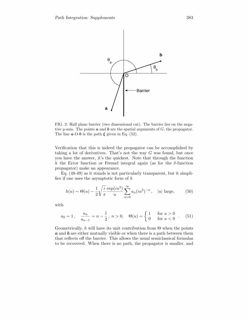
Another exact quantum propagator, found since publication of thisbook, is for the half-plane barrier. In this case the particle is free exceptthat the wave function must vanish on the half-plane defined by y <0, all z. Since there is symmetry in the z direction we can drop totwo dimensions and look only in the x-y plane, with the wave functionvanishing on the negative y-axis. Using the angles defined in Fig. 2, thepropagator, G(b, t;a), is built as follows: Let

ω1 = (θa + θb)/2 , ω2 = (θa − θb − π)/2 ,

µ =√

ab/~t sinω2 , ν =√

ab/~t sinω1 ,

where b = b(cos θb, sin θb), etc. Define the function h as

h(u) ≡ 1√iπ

∫ u

−∞exp(iv2)dv . (47)

Take the particle’s mass to be 1/2. Then

G(b, t;a) =1

4πi~texp

[i(a + b)2

4~t

](48)

×exp(−iµ2)h(−µ)∓ exp(−iν2)h(−ν)

, (49)

where the upper sign corresponds to Dirichlet boundary conditions (theusual conditions for a barrier), but for completeness the lower sign isalso given. The latter would be used for Neumann boundary conditions.


b

a

θb

θa

Barrier

O

FIG. 2: Half plane barrier (two dimensional cut). The barrier lies on the nega-tive y-axis. The points a and b are the spatial arguments of G, the propagator.The line a-O-b is the path ξ given in Eq. (52).

Verification that this is indeed the propagator can be accomplished bytaking a lot of derivatives. That’s not the way G was found, but onceyou have the answer, it’s the quickest. Note that through the functionh the Error function or Fresnel integral again (as for the δ-functionpropagator) make an appearance.

Eq. (48-49) as it stands is not particularly transparent, but it simpli-fies if one uses the asymptotic form of h

h(u) ∼ Θ(u)− 12

√i

π

exp(iu2)u

∞∑

n=0

an(iu2)−n , |u| large, (50)

with

a0 = 1 ,an

an−1= n− 1

2, n > 0, Θ(u) =

1 for u > 00 for u < 0 . (51)

Geometrically, h will have its unit contribution from Θ when the pointsa and b are either mutually visible or when there is a path between themthat reflects off the barrier. This allows the usual semiclassical formulasto be recovered. When there is no path, the propagator is smaller, and


in particular there is an additional factor√~ multiplying it, as will be

seen in detail below.Nevertheless, for the case of no classical path, the term that does

remain, cut down by√~, has an interesting interpretation. Consider

the path (with time variable s)

ξ(s) =

a (t0 − s)/t0 for s ≤ t0b (s− t0)/(t− t0) for s ≥ t0

. (52)

This is the broken line a-O-b (with O the origin). The time t0 ≡ at/(a+b) is chosen so there is no change in speed at the origin. In a sense it’sthe best you can do, given that you want to go from a to b and can’t passthrough the negative y-axis. How close is this to being a good classicalpath? By the Euler-Lagrange equations the first functional derivative ofthe action, S = (1/4)

∫x2 ds, should be zero. Instead, for ξ(s) it is

δS

δx(s)

∣∣∣∣∣ξ(·)

= −(a + b)t

(a + b

)δ (s− t0) 6= 0 (53)

(a = a/|a|, etc.). But ξ(s) does have an extremal characterization: itminimizes S subject to the nonholonomic constraint forbidding transitthrough the barrier. It is easy to evaluate the action along ξ:

S[ξ(·)] =14

[t0

(a

t0

)2

+ (t− t0)(

b

t− t0

)2]

=14

(a + b)2

t. (54)

Comparing this to the half-plane propagator, Eq. (48-49), one sees thatthe phase on line (48) is the action of a path from a to the origin to b.Moreover, the power of ~ appearing on the left of line (48) is the correctpower for two dimensions. But the point that I consider of greatestinterest arises from the rest of G. For the case that there is neither adirect nor a reflected path, the last factor in G is asymptotically

[Shadow

correction

]≡ exp(−iµ2)h(−µ)∓ exp(−iν2)h(−ν)

∼ 12

√i~tπab

[sec

(θa − θb

2

)∓ sec

(θa + θb

2

)].

This has the additional factor√~, mentioned earlier, complete with a

geometrical factor. At this point you might be tempted to say, “Great!I know how to deal with flawed paths: hit them with an extra

√~ and


work out a geometrical term that has information about how deeplyshadowed the endpoints are from each other.” That would indeed bean excellent idea, and you would have rediscovered the beginnings ofthe “Geometric theory of diffraction,” due to Keller, which gives pre-scriptions for a variety of flawed paths. The context is not quantummechanics, but electromagnetic wave propagation, and the power of thetheory is not that you produce the rare exact solution, but rather thatfor geometrical configurations that approximate the exact layouts thisprescription works asymptotically. Thus for a curved barrier with asharp edge, you would calculate the field, or amplitude, in the shadowby using the geometrical diffraction theory prescription, except that youwould have an asymptotic result. As long as the scale of the differencesbetween the true barrier and the ideal one is larger than the asymptoticparameter (wavelength in Keller’s case), the method works.

Infinite dimensional perspective. The result (48-49) was first derivedin a peculiar way: a third point, call it c, was defined in the plane,mutually visible from a and b. Next, the semiclassical propagators froma to c and from c to b were multiplied by one another and the resultintegrated over all appropriate c. (Reflection off the barrier was alsoincluded.) The result, after several asymptotic approximations, was Eq.(48-49), which is an exact solution. I won’t focus on the good fortuneof unjustifiably landing on an exact solution, but instead will elaborateon the asymptotic features. First recall simple facts about asymptotics.Consider the integral

F (λ) =∫ ∞

0eiλf(x)g(x) dx , x ∈ R , λ large. (55)

Usually (e.g., Sec. 11) one studies the “stationary phase approximation,”where for some x0 > 0, f ′(x0) = 0. In that case

F (λ) ∼√

2iπ

λf ′′(x0)eiλf(x0)g(x0) (56)

But if there is no stationary point, that is, |f ′(x)| > 0, ∀x ≥ 0, one cando an integration by parts:

F (λ) =i

λf ′(0)g(0)− 1

iλ

∫ ∞

0dx eiλf d

dx

(g

f ′

)(57)

The new integral on the right in Eq. (57) is like the old one, but carriesan extra 1/λ. Therefore, asymptotically

F (λ) ∼ ig(0)λf ′(0)

. (58)


Two features of this result should be emphasized: first, the asymptoticvalue of the integral is determined by the boundary of integration, inthis case x = 0. Second, the overall scale is cut down by a factor

√λ

relative to its value in the stationary phase case [Eq. (56)].Returning to the path integral, we take the brave perspective that it

is a sum over paths, an infinite dimensional integral,

G (b, t; a) =∫

ΩDx(·) eiS[x(·)]/~ , (59)

where Ω is the domain of functional integration. In the half-plane barriercase, Ω should not include paths crossing the negative y-axis (now downto 2 dim.). Therefore, depending on a and b, there may not be stationary“points” of the action, S in Ω. But Eq. (48-49) tells us what to do inthat case: go to the best point on the boundary of Ω, in this case a paththat just nicks the tip of the barrier, evaluate S for this path, and cutdown the entire result by the square root of the asymptotic parameter—exactly what we did for one-dimensional asymptotics.

I have been tantalized by this connection for more than 20 years, andoff-and-on have tried to put it all together. I will mention a bit more ofwhat I believe must go into the connection, and hope that some enter-prising reader can succeed. (Presumably one should first do this for theWiener integral, where Eq. (59) has rigorous meaning, but I will continueto speak of the path integral and stationary phase approximations.) Then-dimensional generalization of Eq. (57) is

∫

Ωdnx g(x)eiλf(x) =

1iλ

∫

∂Ωdn−1x

g(x)∇f

|∇f |2 eiλf

− 1iλ

∫

Ωdnx∇

(g∇f

|∇f |2)

eiλf (60)

This formula is valid only if ∇f 6= 0 throughout Ω. If ∇f had vanishedin Ω there would be a 1/

√λ multiplying the leading term, rather than

1/λ. Moreover, as before, the first term on the right of Eq. (60) is largerby a factor λ than the second term. Thus the step from 1 dimension ton does not substantially change the asymptotics. The tough part is thecase n = ∞ and establishing that the surface integral gives the desiredterm. One feature of Eq. (60) that only appears in dimension greaterthan one is that the “surface integral” (over ∂Ω) is also subject to thestationary phase approximation, which is why in our half-plane examplethe flaw in the path ξ(t) occurred only on the boundary. As a last remarkI mention that the concept of neutralizer, so useful in asymptotics, canalso be defined for the path integral [31].


3. Coulomb potential and related solutions

In classical mechanics there is a way to make the Kepler (or Coulomb)problem into a harmonic oscillator. It is known as the Kustaanheimo-Stiefel transformation and involves both a change of spatial coordinatesand a change of time variable. The new time is well known in classicalmechanics and is called the “eccentric anomaly” [59]. It is explicitly afunction of a particular path: s(t) ≡ ∫ t

0 dτ/r(τ), with r the radial coor-dinate of the particle. The change of coordinates is more complicated (inthree dimensions) and one must ascend to a 4-dimensional coordinatespace. Nevertheless, it brings considerable simplification to the problemand has been extensively used in classical contexts. Duru and Klein-ert [60, 61] had the lovely idea that once you had a path integral youcould take advantage of the Kustaanheimo-Stiefel transformation since,thanks to Feynman, there were paths, and functions r(t), to work withinside the path integral. Thus for each path you go over to the newtime. With the additional spatial variable, the dynamics becomes thatof the harmonic oscillator, and can be done explicitly.

What these authors and others derived from this formalism is mainlyinformation about the energy-dependent Green’s function. This is be-cause the harmonic oscillator propagator that emerges is for paths in the“new” time, s. Since there is a different s for each path, they cannot allbe gathered into a single physical-time-dependent propagator. For thisreason the goal of an explicit function G(r′′, t; r) ≡ 〈r′′| exp(−iHt/~)|r〉has still not been attained with H the Coulomb Hamiltonian.

Notes

The propagator for the δ-function potential given in Sec. ID 1 wasfound by Gaveau and me [62] using two methods. The simpler wasan expansion over eigenstates; the other was probabilistic and used thepath decomposition expansion. Ref. [63] provides the verification (men-tioned in the text) that the given propagator satisfies the time-dependentSchrodinger equation. Some years earlier Goovaerts, Babcenco and De-vreese [64] had worked out a perturbation expansion for the path integraland applied it to the δ-function potential. They had a particular projec-tion of the full propagator which nevertheless sufficed for the recoveryeigenfunctions and scattering states.

The supersymmetry-based generation of exact propagators was foundby Jauslin [65] and includes as a special case the δ-function.

In more than one dimension the δ-function is invisible; nevertheless,


people in nuclear physics long ago developed singular objects for ideal-ized point scattering centers. Explicit propagators for such “potentials”were found by Scarlatti and Teta [66].

In 1982 there was a conference on “wave-particle duality” in honor ofde Broglie’s ninetieth birthday. Keller’s geometrical diffraction theory[67] provides counterpoint to that theme: historically diffraction was adeciding factor in calling light a wave, but here was Keller with a way tocalculate diffractive fields using rays, something you might be temptedto call particle paths. Because of the importance of paths in Keller’sstory it seemed a good idea to derive his results from the path integral(cf. page 169). Ref. [68] uses a semiclassical approximation to derive theknife-edge (or half-plane) propagator, and noting factors

√~ and the

dominance of the boundary term (of the range of functional integration)I conjectured that this was part of a larger asymptotic theory. The laterrealization that the result was exact led to an additional publication[69]. Apparently the exactness arises because the plane-with-barrier isthe projection of a two-sheeted Riemann surface with the cut locatedalong the barrier [70]. On this surface the motion looks free. This wasexploited by Sommerfeld and for the heat kernel by Carslaw. For someof the history of this problem see [71].

As to getting exact results after lots of approximations, my onlyreaction is to recall the witticism (of Dyson?) that a good physicist isone who makes an even number of mistakes.

Following the original papers by Duru and Kleinert [60, 61] there wasa great burst of activity, some offering alternative demonstrations, andmany extending the technique to other systems. A small part of theliterature is Refs. [72–77].

E. Dissipation and other forced-oscillator applications

You could make the case that the most powerful, effective, and fa-mous applications of the path integral are based on the forced harmonicoscillator. The explicit path integral is given in Eqs. (6.41) and (6.42).As seen in Sec. 21 on the polaron, this comes into play when you havea complicated degree of freedom in contact with a bunch of oscillators,notably the electromagnetic or phonon field, and the coupling to thoseoscillators is linear in the oscillator coordinate. Call the “complicated”degree of freedom r and the oscillator coordinates Qn, n = 1, . . . . Thenthe coupling in the Lagrangian will be

∑fn(r)Qn, with the form of fn

depending on the specific problem. Because∫ Dr(·) is performed last,

as far as Qn is concerned fn(r(·)) is just an external force.


At the beginning of the 1980’s a new application of this idea sprung tolife and has been going strong ever since. The physical system first stud-ied was the Josephson junction, for which the state of a large number ofelectrons is subsumed into a single degree of freedom, the trapped flux ina superconducting ring interrupted by a resistor. At a phenomenologicallevel this flux variable, φ, satisfies an equation of motion

Mφ + ηφ = −dV/dφ + Fext(t) , (61)

where the various parameters, the potential and the external force char-acterize the system, and in particular η is a measure of dissipation. Thecase of particular interest is the “SQUID” (superconducting quantuminterference device) for which the potential V can be made to be a dou-ble well. For the usual situation, having the system variable φ be in oneor the other well means that the supercurrent is flowing in one direc-tion or the other around the loop that constitutes the SQUID. At thequantum level an amazing possibility opened up. This variable couldtunnel, by quantum tunneling, between the wells. This would meanthat a collective variable for perhaps 1011 electrons would behave in apurely quantum fashion.

The theoretical framework for studying this tunneling was to modelthe source of the dissipation, namely to put in the coordinates of thephonons that provided the resistance in the junction. Thus one wouldhave a quantum treatment of the whole system: energy would go fromthe principal degree of freedom to the resistor, but that degree of freedomcould itself go from being in one state (localized on one well) to another(the other well).

The coupling of the phonons to the system degree of freedom couldindeed be set up in the desired form (linear forcing) and the tunnelingcalculated. The Lagrangian used by Caldeira and Leggett [78] was

L =12Mq2 + V (q) +

12

∑α

mαx2α +

12

∑α

mαω2αx2

α + q∑α

cαxα ,

with q the dynamical variable (ultimately identified as φ), xα thephonon coordinates, and cα characterizing the coupling. One of theimportant physical properties that played a role in the results was thephonon spectrum, embodied in cα and implicit in

∑α. Simplifications

were also introduced, for example replacing q by a two-state variable,giving the entire system the name “spin-boson model.” As for the po-laron, one first does the path integral for the xα, then sandwiches thepropagator between states of the oscillators, typically the ground states.After this the functional integral involves the original Lagrangian in q


plus the result of all the completed integrations, which can now dependonly on q. This gives an action contribution (the imaginary part of thelogarithm of the result of all those integrals), which is an effective self-interaction of q. This self-interaction is non-local in time (as for thepolaron) and represents the back-reaction of the field of oscillators onthe motion of the variable of interest, q.

By now there are books and review papers that not only describe theSQUID application but also the many other situations where a systeminteracts with a heat bath, and nevertheless retains quantum properties.Typically, but not always, energy concentrated in the principal degreeof freedom leaks into the oscillator modes, i.e., there is dissipation. Iwill not document the history of this application, but only cite sourceswhere the reader can get into the subject [79–83]. More on this (andother) literature appears in Sec. II.

Meanwhile, other applications of Feynman’s forced-oscillator integra-tion continue to flourish. The polaron has historically had a special role:even those content to go through life without the pleasures of path inte-gration will concede that for the polaron you can compute things usingthe path integral that are difficult to get by other methods. A reviewby Devreese [84] summarizes the polaron situation as of 1996. His groupin Antwerp continues to work in this area [85, 86] and to use the pathintegral for other physical systems as well [87].

I recently used the forced oscillator technique for a condensed mat-ter application, the quantization of discrete breathers. These are latticeexcitations involving strong nonlinearity. Classically such localized os-cillations are a kind of stationary soliton and can live forever [88]. Bymassaging the system it can be brought to a form suitable for the forcedoscillator machinery, and the quantum stability of the system can bestudied [89]. Let me pass on one lesson I learned from this: trust no one(including me). Even if you take Eqs. (6.41) and (6.42) as correct (whichI believe they are), you still have several Gaussian integrals to do. Thenthere’s usually an analytic continuation and a double integral variouslywritten

∫T

0 dt∫

T

0 ds or∫

T

0 dt∫ t0 ds, which brings in another factor two. For

the serious people, I trust them to have gotten all these signs and factorsright in their research papers—but not in their lectures! In my work,[89], I wasn’t sure of all these factors and signs until I found a way inwhich the effective action could be used to recover the spectrum of theoriginal system, and when it agreed with that spectrum calculated byother means, I stopped worrying. By the way, symbolic manipulationprograms, at least in the hands of my collaborators, were of no help.(See also the “comment on page 173” in Sec. III.)


F. Mathematical developments

Making proper mathematics out of the path integral has been a dreamsince Feynman’s first paper on the subject. Like Newton and Dirac,mathematical innovators in quest of physical knowledge, Feynman knewhow to get things right even if not all the mathematical i’s were dotted.And perhaps, as for the inventions of his predecessors, a full mathemat-ical theory will follow. In Sec. 9 I mentioned work of DeWitt, Albev-erio, Hoegh-Krohn and Truman, all of them having this goal in mind.Cameron (cited in the Sec. 9 notes) had found that the path integralcould not provide a bona fide measure. But if you weaken the demands,redefine “bona fide,” new possibilities open. For example, Tepper andZachary [90] have relaxed the need for countable additivity in the mea-sure and find a useful object nevertheless. Another tack has been takenby Fujiwara and Kumano-go [91, 92], who focus on the properties of thetime-sliced expression for the propagator, establishing classes of func-tions for which that is meaningful, and developing asymptotics in thatcontext as well. Yet another approach is by Nakamura [93], who has beenusing non-standard analysis [94], taking advantage of that framework’sability to with deal with explicit infinities and infinitesimals.

One avenue that appeals to me physically (although it has receivedonly slight attention [95]) would start from the checkerboard path in-tegral. For this there is a well defined measure. Then find its non-relativistic limit, which as discussed in Sec. I C, is the usual path inte-gral.

G. Electromagnetism and other PDE’s

In Sec. 20 I showed how the path integral could be applied to ge-ometrical optics, basically to the wave equation, where the big step isto get rid of the ∂2/∂dt2 by looking at a fixed frequency. Then, byhand, I inserted an artificial time variable, so as to make it look like theSchrodinger equation. My goal was aesthetic, to show the common fea-tures of Fermat’s principle of optics and the semiclassical approximationof quantum mechanics.

It turns out that there’s a practical side to this resemblance as well.People really do use the path integral for the solution of partial differen-tial equations other than the Schrodinger and diffusion equations. Fur-thermore, in some of these applications the “time” variable has a clearphysical meaning as the spatial variable along the direction of propaga-tion (analogous to the eikonal approximation). Quite a few papers on


sound transmission in channels have appeared and Refs. [96–98] shouldhelp you find your way into this field. More recently, Schlottmann [99]pioneered the use path integral methods in geology. This is a difficultwave transmission problem, since not only is the medium nonuniform,but it’s that uniformity that you are interested in. Impressive results ofin this area have been obtained by Fishman [100, 101], whose path inte-gral methods for the Helmholtz equation can provide a detailed pictureof geological structure, especially useful for oil exploration.

For electromagnetism path integral methods have been used to findthe low order modes of complicated waveguides [102, 103]. This is notthe time-dependent propagator, but an application of the method of Sec.7, taking advantage of the dominance of the lowest mode for large imag-inary times. As a practical method this was first proposed by Donskerand Kac in the 1950’s, and I believe they even did numerical calculations(punch cards and all). There have also been significant extensions of raytracing techniques [104].

H. Homotopy

For diverse reasons, there are physical systems where the homotopyof the coordinate space is not trivial. As described in Sec. 23, the pathintegral provides an intuitive approach to multiple connectedness, sincehomotopy theory, like the path integral, focuses on paths, with its start-ing point being an equivalence relation among them.

The phase that can be associated with winding number, discussedin Sec. 23.1, has as its most common application the Aharonov-Bohmeffect. The path integral/homotopy perspective goes back, as far as Iknow, to my thesis and its extension (for the Aharonov-Bohm effect),Ref. [105]. A physical arena where this frequently arises is the mesoscopicsuperconducting ring, a recent paper on this being [106]. See also [107,108]. A closely related way to think about the richness permitted by themultiple connectedness is in terms of the Berry phase.

These phenomena also are present in non-Abelian gauge theories andhave been studied by Sundrum and Tassie [109].

A somewhat different application came up in connection with theconcept of anyons. As Laidlaw and DeWitt realized (Sec. 23.3), in twodimensions you can get additional kinds of quantum statistics, not justfermions and bosons. Such excitations were proposed in the attemptsto understand high temperature superconductivity [110, 111]. (See alsoCanright’s lectures in [112].) Ultimately, in the realm of superconductiv-ity these ideas were put aside, but other applications have been proposed.


I. And more . . .

Sec. 32 of this book is entitled “Omissions, Miscellany and Preju-dices,” and represented my effort to get just a bit more material underthe wire of a publication deadline. In this respect, little has changedin 20+ years. Here too I present just the briefest guide to a number ofdevelopments that have caught my attention.

1. Variational corrections to the classical partition function

An approximation for the partition function was independently de-veloped by Feynman and Kleinert [113] and by Giachetti and Tognetti[114] in the mid 1980’s. They sought quantum corrections to the semi-classical partition function, making use of quadratic approximations tothe potential energy function. These approximations were not merelythe lowest quadratic fit, but were themselves found through a variationalprinciple. In both cases, the initial publication was followed by severalothers of which a small sample is [115, 116].

2. A particular numerical approach

There has been an enormous amount of numerical work using thepath integral (usually its real-valued analytic continuation), includingcases where fermion statistics create a severe sign problem. I will notreview this, although lectures by Pollock can be found in [112] and otherliterature is given in Sec. II. Here I want to mention one scheme thathas not been pursued on an industrial scale and which at first sounds asif it shouldn’t work.

Since the path integral is the sum G =∫ Dx(·) exp(iS/~), you

could imagine a change of variable to a one dimensional integral G =∫dS Ω(S) exp(iS/~), where Ω(S) is the number of paths with action

S. It’s an ambitious change of variables and requires real belief in thepath-sum concept. By this method all the trouble is transferred to theevaluation of Ω(S). Creswick [117] proposed this idea and worked outa number of examples with numerical and analytic estimates for Ω(S).My first impression was that the roughness of the significant paths mit-igated against having any reasonable limit for Ω(S) as the time-slicingmesh went to zero. However, although the limit may not exist, for anyparticular time-slicing (say N “slices”) Ω can be evaluated, and as afunction of N it is possible to define sensible properties. In a way this


reflects the way I believe one should deal with path integral subtleties:go back to the multiple integral,

∫ ∏N

n=1 dxn. Or as Kac is reputed tohave said: when in doubt, discretize.

3. Semiclassical approximations for coherent states

In molecular systems there occasionally develop large magnetic mo-ments. Such a moment may have more than one preferred orientationand there will be a quantum tunneling amplitude for transiting betweenclassically degenerate states. Given the largeness of the moments itwould be reasonable to expect semiclassical tunneling calculations tobe helpful. One would also expect that the coherent state formalism,which has often been used to represent such degrees of freedom, wouldbe a good vehicle for such a calculation, especially since its phase spaceinterpretation brings it close to a semiclassical language. Nevertheless,considerable difficulties were encountered. In recent work more reliabletechniques have been developed and I refer the reader to [118] as anentry into this literature.

4. Chaos and order

The use of the path integral in studying quantum chaos was estab-lished with Gutzwiller’s trace formula [119]. In many places in this book[e.g., Eq. (13.25)] the propagator is approximated by a sum over classicalpaths, which means that for given endpoints in G(b, t; a) there may beseveral solutions of the classical equations of motion. The propagatoris then given by their sum, with interesting possibilities for interferenceand other quantum phenomena.

For a classically chaotic system the number of solutions to the two-time boundary value problem associated with G(b, t; a) generally growsexponentially with t. If t is long enough you’d therefore expect a break-down in the semiclassical approximation. This is not what happens.Even for long times a great deal of useful information can be extractedfrom the propagator.

By taking a trace of the propagator and applying a stationary phaseapproximation, Gutzwiller focused on the periodic orbits. This is be-cause the trace forces initial and final positions to be the same while thestationary phase approximation takes care of matching the momentum.These periodic orbits can be quite long; nevertheless, their contributionto the propagator reliably gives information about the quantum system,


for example concerning the density of states. The literature on this sub-ject extensive. A convenient source, with many references, is [120] byCvitanovic et al., which is directly available on the web (the Gutzwillertrace formula is in Chapter 30).

Better than expected accuracy in the path sum for a classically er-godic system was also seen by Heller and Tomsovic [121]. They studied a“stadium billiard” (a free particle in a kind of elongated oval) and foundthat even when there were 30000 paths to add, a great deal of quantuminformation survived intact. An important technical point is that theywere not actually looking at the propagator as a function of its positionendpoints; rather they sandwiched it between coherent states, therebysmoothing the singularities that would otherwise arise from caustics ofthe motion. One feature that helped me understand this discovery wasthat although in the two-dimensional coordinate space the paths crossedand re-crossed each other, in phase space there is lot more room [122].Another path-integral oriented approach to the smoothing of causticsingularities, especially in chaotic situations, is by Takatsuka [123].


II. LITERATURE

The library of path integral books has grown substantially since thepresent volume was first published. There are textbooks, conferenceproceedings and review papers. Books focussed on other subjects, forexample quantum field theory, will often have introductions to the pathintegral. Below is a partial list of publications since this book appeared.I have not tried to be comprehensive.

A. Texts and review articles

Roepstroff, Path Integral Approach to Quantum Physics: An Introduc-tion [124]. Mathematically careful, but not at the expense of goodinstruction.

Kleinert, Path Integrals in Quantum Mechanics, Statistics and Poly-mer Physics, and Financial Markets [15]. Covers an impressivelywide range of topics, including the Duru-Kleinert Green’s functionsolution discussed in Sec. I D 3.

Kac, Integration in Function Spaces and Some of Its Applications [125].Notes for lectures Kac gave in Italy. Marked by his usual livelystyle, although they may be hard to locate.

Wiegel, Introduction to Path-Integral Methods in Physics and PolymerScience [71]. Emphasizes polymer applications and is a readableand informative volume.

Gutzwiller, Chaos in Classical and Quantum Mechanics [119]. Exten-sive coverage of quantum chaos, with the path integral serving asa (very effective) tool.

Glimm and Jaffe, Quantum Physics: a Functional Integral Point of View[126]. The work of these authors played a part in the developmentof “constructive quantum field theory,” a subject for which thefunctional integral is used in a mathematically rigorous way.

Weiss, Quantum Dissipative Systems [127]. An introduction with manyapplications to the use of functional integration in handling dissi-pation in quantum systems.

Dittrich, Hanggi, Ingold, Kramer, Schon and Zwerger, Quantum transportand dissipation [83]. A collection of articles offering introductionsto the fields indicated by the title.


Cerdeira, Lundqvist, Mugnai, Ranfagni, Sa-yakanit and Schulman, Lec-tures on Path Integration: Trieste 1991 [112]. A collection ofdiverse lectures at a pedagogical level, given at a workshop at theICTP, Trieste. As a co-organizer I wanted the topical coverage tobe an update of sorts for this book.

Roncadelli and Defendi, I Camini di Feynman [128]. A pedagogical workin Italian, also reflecting contributions of the authors to the field.

Choquet-Bruhat and Dewitt-Morette, Analysis, Manifolds and Physics[129]. Introduction to many mathematical methods in physics,with in-depth treatment of the path integral.

Ranfagni, Mugnai, Moretti and Cetica, Trajectories and Rays: The Path-Summation in Quantum Mechanics and Optics [130]. A path ori-ented approach to problems in quantum mechanics and optics.

Freidlin and Wentzell, Random Perturbations of Dynamical Systems[131]. Functional integrals as well as other probabilistic methods,with emphasis on asymptotics.

Steiner and Grosche, A Table of Feynman Path Integrals [132]. A usefulcompendium.

Books on quantum field theory. As the reader may have guessed, quan-tum field theory is not my favorite arena for path integration. Butfor lots of other people it is (“Let a hundred flowers bloom, . . . ”).A few of the more well-known texts that make extensive use ofpath integration are Popov [133], Ramond [134], Itzykson and Zu-ber [135], Faddeev and Slavnov [136], and Rivers [137].

Review articles

Leggett, Chakravarty, Dorsey, Fisher, Garg and Zwerger, Dynamics ofthe dissipative two-state system [81]. Justification and use of thespin-boson model.

Grabert, Schramm and Ingold, Quantum Brownian Motion: The Func-tional Integral Approach [82]. Pedagogical presentation at an ad-vanced level.

Ceperley, Path integrals in the theory of condensed helium [138]. Re-views an extensive literature in which Feynman’s original idea ofhow to deal with Helium (as a classical model of interacting “poly-mers”) is implemented with intensive numerical computation.


Khandekar and Lawande, Feynman Path Integrals: Some Exact Resultsand Applications [139]. Quite a few explicit path integrals includ-ing some that are nonlocal in time.

Gaspard, Alonso and Burghardt, New Ways of Understanding Semiclas-sical Quantization [140]. Extensive background on semiclassicalmethods, with the path integral playing a prominent role. Ap-plication to quantum chemistry, including reactions and chaoticscattering. Higher order (in ~) corrections to the Gutzwiller traceformula.

Littlejohn, The Semiclassical Evolution of Wave Packets [141]. Notreally path integration, but a trove of information and perspectiveson semiclassical approaches.

Shankar, Renormalization-group approach to interacting fermions [142].Extensive use of the path integral for fermions (something notcovered in this book) to study interaction between them. Thefermion path integral uses Grassmann variables and these too areintroduced in this article.

B. Conference proceedings

In 1983 the first of the “Path integrals from meV to MeV” conferencestook place, organized by Akira Inomata, in Albany, New York. Sincethen, every three or four years there has been another such meeting,although the name of the conference has evolved. The original titlewas selected to emphasize physical phenomena, in contrast to severalmathematically oriented meetings in the then recent past. Today wealso have mathematicians coming and the limits meV and MeV havevariously been replaced by quarks, peV, quantum information, TeV,galaxies and cosmology. The proceedings give an overview of the range ofapplications, although the mode of publication has varied from meetingto meeting and some of the proceedings may be hard to track down.The meetings: Albany 1983 [143], Bielefeld 1986 [144], Bangkok 1989 [145],Tutzing 1992 [146], Dubna 1995 [147], Florence 1998 [148], Antwerp 2002 [149],Prague 2005 [150].

Besides the meV/MeV series, there have been conferences and work-shops where the path integral played a significant role. These can be auseful way to survey activity in the field, although these days people aremore inclined to search the web than to get off their chairs and go tothe library. A non-exhaustive list of conferences is [151–154].


III. PAGE BY PAGE COMMENTS AND ERRATA

Conventions: references to “Sections” 1 through 32 are to sectionsof this book (a.k.a. chapters). Equation numbers with periods, (n•m),refer to equations in the book; those consisting of a number alone referto the supplement. Sections of the supplement have labels beginningwith Roman numerals.

• Sec. 1, page 4, Eq. (1.11); elaboration of the associated footnote.Show that

f(λ) ≡ eλAe−λ(A+B)eλB = 1− 12λ2[A,B] + . . . .

Evaluate df/dλ = Af − eλA(A+B)e−λAf + fB. Clearly f ′(0) = 0. Thesecond derivative is f ′′ = Af ′−eλAA(A+B)e−λAf+eλA(A+B)Ae−λAf+f ′B. Since f ′(0) = 0, the only term surviving is f ′′(0) = [B, A].

• Sec. 6, page 39, solution to part (b), exercise at top of page.The correct form of the propagator is

G(x2, t; x1, 0) =[ m

2πit

]3/2exp

im

2

[ω

2cot

ωt

2

(B × r

)2

−ωB · x2 × x1 +1t

(B · r

)2]

For more on this propagator, see Glasser [155]. When there are constantelectric and magnetic fields on a lattice, although the fields share theunderlying periodicity, the potentials giving rise to those fields do not.See [156] for a path integral treatment of this situation.

• Sec. 6, page 40, discussion following Eq. (6.43).Eq. (6.43) asserts

G(b, t; a) =

√1

2πit

[ei(b−a)2/2t − ei(b+a)2/2t

], Sec. 6, Eq. (6.43)

where G is the propagator for a particle confined to x > 0, x ∈ Rbut otherwise free (V = 0). The justification (in Sec. 9) uses what isessentially the method of images. I complain on page 40 that it is an“embarrassment to the purist” that I did not present a sum-over-pathsderivation. Shortly after the book was published, Goodman [26] gavethe following purely path integral argument.


As usual write

G(b, t; a) =∑

exp(iS/~) ,

with the sum taken over x(·) such that x(0) = a, x(t) = b andx(s) > 0, for 0 ≤ s ≤ t. We also define the free propagator, de-noted G0(b, t; a), which is the sum over paths from a to b in time t,but without the restriction. The difference between G and G0 is thesum over paths that have at least once entered the region x < 0,but returned to b nevertheless. Call these “forbidden” paths. ThenG(b, t; a) = G0(b, t; a)−∑

forbdden pathsexp(iS/~).

Consider a forbidden path, x(·). There will be a last time, t`, forwhich x(t`) < 0. Define the path x(·) as follows

x(s) =

x(s) for s < t`−x(s) for s > t`

.

The final position of x(·) is thus−b rather than b. The difference betweenS(x(·)) and S(x(·)) goes to zero as the mesh for time-slicing goes to zero,because the flip in direction at t` has negligible impact on S. On theother hand, the set of paths x(·) includes all paths from a to −b in timet. As a result the sum,

∑forbdden paths

exp(iS/~), is in fact equal to the freepropagator from a to −b. Therefore G(b, t; a) = G0(b, t; a)−G0(−b, t; a).

• Sec. 7, page 47, Eq. (7.22).An even easier way to do the integral. You want to evaluate

f(c) =1√b

∫ ∞

0dy exp

(− c2

y2− y2

)Sec. 7, Eq. (7.22)

Rewrite the integrand slightly,

f(c) =1√b

∫ ∞

0dy exp

[−

(y − c

y

)2

− 2c

]=

1√b

e−2c ψ(c) , (62)

where ψ(c) ≡ (1/√

b)∫∞0 dy exp

[− (y − c/y)2

]. Now compute

∂ψ

∂c=

∫dy 2

[1− c/y2

]e−(y−c/y)2 . (63)

But this derivative is zero, since the individual terms in square bracketgive the same integral, as can be seen from the substitution x = c/y. Tofinish, set c = 0 to find ψ(c) = ψ(0) =

√π.


• Sec. 9, page 54, prior to Eq. (9.4).The calculation of u(j, N) of Eq. (9.4) uses the assumptions α2/N =O(1) and j2/N = O(1). Note too that for finite N Eq. (9.4) does nothold in the extreme tail of the distribution.

• Sec. 9, page 63, new exercises.Exercise: You enter a casino with $100, intent upon walking out witheither nothing or $1000. Assuming you place a series of $1 bets using afair coin (tell me where to find this casino . . . ), use the methods of thissection to compute the probability of each final state.Exercise: Evaluate E

([x(t+δ)−x(t)]2

δ

).

• Sec. 12, page 81, Eq. (12.9).For the specific case L = mx2/2 − V , Eq. (12.9) takes the simple formφ + V ′′φ + λφ = 0. See Eq. (12.18).

• Sec. 12, page 82, Eqs. (12.17) and (12.18).The approximation Eq. (12.17) is appropriate for the intended demon-stration. But it could be sharpened if for example one wanted to betterestimate the interval during which the path is a true minimum. Eq.(12.18) still holds (with x(t) an Euler-Lagrange equation solution), butEq. (12.19) need not.Justification of the approximation: If the magnitude of the force, F (x) ≡−dV/dx, is bounded (say |F | ≤ Fmax) then it is easy to show that Eq.(12.17) is good to O(T 2). The equation to solve is x = −dV/dx withx(0) = a, x(T ) = b. Let the true solution be x(t) = a+(b−a)t/T +u(t),so that u(0) = u(T ) = 0 and u = F (x). We want to bound u. Firstintegrate to t ≤ T . u(t) = u(0)+

∫ tF (x(s))ds (lower limits of integration

are 0 throughout). This implies |u(t)| ≤ |u(0)|+ tFmax ≤ |u(0)|+TFmax.Since u(t) =

∫ tu, |u(t)| ≤ (|u(0)|+ TFmax)T . It remains to bound u(0).

Integrate the equation for u twice: u(t) = tu(0)+∫ t

dt′∫ t′

dt′′ F (x). Sett = T and use u(T ) = 0. This implies |u(0)| ≤ (1/T )

∫T

dt′∫ t′

dt′′Fmax =FmaxT/2, which shows that u = O(T 2).

• Sec. 12, page 90, “ THEOREM.”In quoting the theorem I neglected to define “strong minimum.” Theactual terminology used in Bliss [157] is “strong relative minimum.”The distinction between strong and weak refers to how broad is theclass of paths relative to which this is a minimum. Earlier on page90 I allude to the pitfalls of lapses from full rigor in the subject ofvariational principles, so that thus warned I won’t try to convey allthe subtleties of Bliss’s presentation in these pages. His book, [157],


R

Original contour

New contour

−φ

Countour whose contributionvanishes for R → ∞

Complex y plane

FIG. 3: For the “comment on Sec. 13, page 99.”

is part of a series, the Carus Mathematical Monographs, published bythe Mathematical Association of America, which offers readable andenjoyable introductions to a variety of topics.

• Sec. 13, page 94, material following Eq. (13.8).If Secs. 11 and 12 have not been read at this point, it is sufficient tobegin at the paragraph preceding Eq. (12.29) and continue through theparagraph containing Eq. (12.45).

• Sec. 13, page 99, discussion following Eq. (13.20).Fig. 3 may be useful for following the argument on page 99. The inte-grand in (13.20), with α = eiφ, can be made to look like that in (13.12),but with the path of integration along the ray 0 to ∞ · e−iφ (the “Newcontour”).

• Sec. 13, page 104, paragraph following Eq. (13.42).Concerning the slope of the curves in Fig. 13.1, for small E and forthe lowest curve, T (E) is given by (2π/ω)

[1− (3/4)(λE/ω4) + O(E2)

].

The T versus E curve can be much richer than is illustrated in Fig.13.1, and can bend around, connecting paths with different numbers ofturning points. Doing the Exercise on page 105 will illustrate this point.Examples are given in [158].


• Sec. 14, page 110, Eq. (14.12).The σ defined here and that defined in Sec. 6 differ by a factor ε/i~, i.e.,

σSec. 6 =ε

i~σSec. 14 .

• Sec. 18, page 155, Eqs. (18.27), (18.28a) and (18.28b).A trivial example with which to see the interplay of path absenceand imaginary time is the free particle. Eq. (7.18) has the sameform as Eq. (18.27). An exact integration yields [Eq. (7.20)] G(E) =√

m/2E exp(i|x|

√2mE/~

), but one could as well arrive at this result

by a stationary phase approximation, with the stationary point in time[for Eq. (18.28)] given by tstationary = −x

√m/2E. Now consider E < 0,

for which the free particle does not have classical paths. This givesus what we want: pure imaginary “stationary” time and exponentialdropoff in space.

• Sec. 21, page 173.Integrals of the form

∫ T0

∫ T0 and

∫ T0

∫ t0 make their appearance on this and

nearby pages. Moreover they come with factors ±2±n. A confession: Icannot promise you that I got it all right. I recently did a calculation ofthis sort and found that not only could I not rely on my own presentation,but as far as I could tell Feynman gave different versions in differentplaces, and that other authors generally are not explicit about theseterms. In my own recent calculation I could only be sure when I founda different way of getting the system’s spectrum and it agreed withwhatever signs and factors I’d finally convinced myself to use (it alsohelped that Denis Tolkunov worked with me on this).

• Sec. 21, page 181The reference given for the work of Donsker and Varadhan may not beeasily accessible. A web search for their names plus “large deviations”will turn up many sources. The fourth in their series of articles is in thejournal Comm. Pure Appl. Math. vol. 36 (1983), 183–212. I believe asignificant stimulus to the large deviation quest was work of Friedbergand Luttinger [159] on disordered systems, which, at a heuristic level,arrived at results similar to those of Donsker and Varadhan.

• Sec. 22, page 188, just after the first paragraph.Feynman suggested the use of time-ordered products for the Dirac equa-tion in [160]. But he apparently did not consider them practical sinceaccording to [161] they would demand delving into “the geometricalmysteries involved in the superposition of hypercomplex numbers.”


• Sec. 23, page 195, paragraph beginning, “The degree of pathology. . . ”In this paragraph, “entertaining” properties of the Jacobi θ-function areexhibited, based on its zeros. But you need to know that there is atleast one zero per quasi-periodic cell:Exercise: Show that θ3(z0, t) = 0, with z0 = π(1 + t)/2.The fundamental theorem for θ-functions is Eq. (23.13). It is worthgoing through its derivation:Exercise: The Poisson summation formula (for appropriate f) is

∞∑n=−∞

f(x + n) =∞∑

k=−∞exp(2πikx)

∫ ∞

−∞dy f(y) exp(−2πiky) .

Find a function, f , such that this formula leads to Eq. (23.13).For the solution to this exercise as well as a great deal more entertain-ment, I recommend the book of Bellman [162], where the field of ellipticfunctions is heralded not only as entertaining, but enchanting and won-drous as well. (See also the end of Sec. III.)

• Sec. 23, page 197, after the theorem.In the proof I show one of the properties of an equivalence relation,transitivity. The other properties are reflexivity, f ∼ f , and symmetry,f ∼ g ⇒ g ∼ f . If this is your first exposure to homotopy theory, itwould be worth writing down the steps to prove these other properties.

• Sec. 23, page 203, Definition and THEOREM.For an illustration of a covering projection see Fig. 23.1, page 193.

• Sec. 23, page 211, second paragraph of Sec. 23.4.I needed to be more careful in my statement. The condition that thefunction must vanish at the endpoints of the interval (plus certain regu-larity conditions) does define H sufficiently to make it self adjoint. See[163], §119. But when you do not demand that the function vanish, thereemerges the additional richness discussed in this section, in particularthe absence of essential self adjointness and the possibility of definingthe operator in many ways.

• Sec. 24, page 220, following Eq. (24.25)For the record, the Laplacian on SU(2) is

∆ =∂2

∂θ2+ cot θ

∂

∂θ+

1sin2 θ

(∂2

∂φ2+

∂2

∂ψ2− 2 cos θ

∂2

∂φ∂ψ

).


• Sec. 25, page 234, after line 5 (end of continuing paragraph).Continuing the discussion of this paragraph, it’s worth being more ex-plicit. For Kruskal coordinates, u ∼ cosh(t/4M) and v ∼ sinh(t/4M).Consider exp(t/4M) with t → t − iπ/κ. Then exp(t/4M) →− exp(t/4M), since κ = 1/4M . Thus u → −u and v → −v. Thepoint (−u,−v) is B′ in Fig. 25.4.

• Sec. 27, page 244, Eq. (27.9).Here is a proof of Eq. (27.9): Let [[A,B], A] = [[A,B], B] = 0. Then

eA+B = eAeBe−[A,B]/2 = eBeAe+[B,A]/2 Sec. 27, Eq. (27.9)

Lemma 1. [A,Bn] = nCBn−1, where C ≡ [A, B].Proof by induction: [A,Bn+1] = B[A,Bn] + [A,B]Bn, which by the in-ductive hypothesis is BnCBn+[A,B]Bn, and which by our assumptionsand definitions is (n + 1)CBn. The case n = 1 is obviously true.Note that [B,An] = −nCAn−1, by interchange of letters.Lemma 2. [A, eλB] = λCeλB

To prove this, expand the exponential, use Lemma 1, and re-sum.Now define

g(x) ≡ e−xAex(A+B)e−xB .

Take dg/dx. By straightforward manipulations and the use of Lemma 2this becomes dg/dx = e−xA[B, ex(A+B)]e−xB, which by Lemma 2 (withan interchange of letters) leads to dg

dx = −xCg (also using the fact thatC commutes with everything). Now integrate the differential equationfrom 0 to 1 to get g(1) = exp(−C/2). This is the desired result (proofattributed to Glauber).

I think of Eq. (27.9) in terms of the Baker-Campbell-Hausdorff series.This is an expression for exp (λ(A + B)) in the case where [A,B] need notcommute with A and B. In this series, terms with powers higher than λ2

all involve commutators of A and B with [A,B]. So Eq. (27.9) is simplya truncation of the Baker-Campbell-Hausdorff series. For informationon (including a derivation of) this series see [164–166].

• Sec. 27, page 245, Exercise.Solution to the exercise: One possibility is v(z) = 1 − |z|2/2. By Eq.(27.12) it is only necessary to show that

∫exp(−|z|2/2)znv(z)d2z = 0,

for all n. Polar coordinates will help.


• Sec. 27, page 247, discussion following Eq. (27.21).Cross reference: the propagator “obtained earlier in this volume” is Eq.(6.38). Note that the “very easy” way to do this path integral only worksfor the harmonic oscillator.

• Sec. 27, page 248, just after Eq. (27.28).Eq. (27.28) is often written without explicit “time-slicing” as

G(zf , t; zi) =∫ zf ,t

zi,0d2z(·) exp

i

∫ t

0dτ

[i

2

(z∗

dz

dτ− dz∗

dτz

)−H(z∗, z)

]

• Sec. 28, Eq. (28.3).For completeness I give an indication of how Eq. (28.3), the expectednumber of particles in each state, is derived. For a fixed number, N ,of particles, the canonical partition function is ZN =

∑α exp(−βEα),

where α labels states and I have dropped the superscript (C) specifyingthe sphere-configuration that appears in Eq. (28.3). (Recall that thecanonical partition function pertains to a system in contact with a heatreservoir at temperature 1/β.) Since this is an ideal gas (no interac-tion between particles), its states can be labeled α = (n1, . . . , nk, . . . ),where nk is the number of atoms in the one-particle state k. The to-tal energy is Eα =

∑k nkεk, with εk the kth one-particle energy. The

constraint N =∑

k nk makes the partition function sum difficult so onegoes to the grand canonical ensemble. For the latter ensemble one hasa reservoir of particles with chemical potential µ and partition functionZGC =

∑N ZNeβµN . The probability of finding a particular state and

a particular number of particles is thus e−βEα+βµN/ZGC. The chemicalpotential is then fixed so that the weaker requirement, N =

∑k〈nk〉,

is satisfied, with the expectation taken with respect to the probabilityjust indicated. One can now calculate the expected occupation of aparticular one-particle state:

〈nk〉 =∑

N,α

nk Pr (state-k occupied by nk particles) =−1β

∂

∂εklog ZGC .

All sums are geometric and one gets

〈nk〉 =1β

∂

∂εklog

(1− e−β(εk−µ)

)=

1eβ(εk−µ) − 1

.

• Sec. 23, p. 195 (out of order).Solution to the new exercise for page 195: f(x) = exp(−ix2/πt).


References and endnotes for the supplements

[1] Those with a mathematician’s aesthetic will recoil at the idea of goingthrough a tedious expansion to derive Eq. (13), after having done a sim-ilar calculation to derive Eq. (6). The product on the right-hand-side ofEq. (13) can be written exp(λB/2) exp(λA/2) × exp(λA/2) exp(λB/2),with the first and second pairs giving exp(λ(A + B)/2 by Eq. (6), andwith corrections of order λ2. Because the order of A and B is reversedin the two pairs, these corrections will be equal but of opposite sign.Putting the corrections next to each other, which can be done to thislevel of precision, allows the O(λ2) corrections to cancel, leaving an errorthat is O(λ3).

[2] R. P. Feynman, Space-Time Approach to Non-Relativistic Quantum Me-chanics, Rev. Mod. Phys. 20, 367-387 (1948).

[3] B. Gaveau, E. Mihokova, M. Roncadelli, and L. S. Schulman, Path inte-gral in a magnetic field using the Trotter product formula, Am. J. Phys.72, 385-388 (2004).

[4] B. Gaveau and L. S. Schulman, Sensitive terms in the path integral: or-dering and stochastic options, J. Math. Phys. 30, 2019-2022 (1989).

[5] L. S. Schulman, Selected Topics in Path Integration (1993), in [112].[6] W. Janke and T. Sauer, Properties of higher-order Trotter formulas,

Phys. Lett. A 165, 199-205 (1992).[7] L. S. Schulman, Introduction to the Path Integral (1988), in [167].[8] D. W. McLaughlin and L. S. Schulman, Path Integrals in Curved Spaces,

J. Math. Phys. 12, 2520-2524 (1971).[9] T. Ichinose and H. Tamura, On the Norm Convergence of the Trotter-

Kato Product Formula with Error Bound, Operator Theory: Adv. Applic.126, 149-154 (2001).

[10] J. Hull, Options, Futures, and Other Derivative Securities (Prentice Hall,Englewood Cliffs, New Jersey, 1993), 2nd ed., chapter 10.

[11] B. B. Mandelbrot, Fractals and Scaling in Finance: Discontinuity, Con-centration, Risk (Springer, New York, 1997).

[12] B. B. Mandelbrot, The Fractal Geometry of Nature (W. H. Freeman andCompany, New York, 1983).

[13] J.-P. Bouchaud and M. Potters, Theory of Financial Risks (CambridgeUniv. Press, Cambridge, 2000).

[14] R. N. Mantegna and H. E. Stanley, An Introduction to Econophysics(Cambridge Univ. Press, Cambridge, 1999).

[15] H. Kleinert, Path Integrals in Quantum Mechanics, Statistics & PolymerPhysics, & Financial Markets (World Sci., Singapore, 2004), 3rd ed.

[16] L. F. Abbott and M. B. Wise, The Dimension of a Quantum-MechanicalPath, Am. J. Phys. 49, 37-39 (1981).

[17] F. Cannata and L. Ferrari, Dimensions of relativistic quantum mechanicalpaths, Am. J. Phys. 56, 721-725 (1988).


[18] H. Kroger, Proposal for an experiment to measure the Hausdorff di-mension of quantum-mechanical trajectories, Phys. Rev. A 55, 951-966(1997).

[19] H. Kroger, Generalized Aharonov-Bohm effect, homotopy classes andHausdorff dimension, Phys. Lett. A 226, 127-134 (1997).

[20] H. Kroger, S. Lantagne, K. J. M. Moriarty, and B. Plache, Measuring theHausdorff dimension of quantum mechanical paths, Phys. Lett. A 199,299-303 (1995).

[21] It may be overkill, but let me explain this point in detail. Imagine thatfor fixed N (the time-slicing parameter) we also discretize space andwrite the path integral as an enormous sum. For small enough mesh (andlarge enough spatial cutoff) this sum approaches the integral, because afinite slicing of the path integral is an ordinary Riemann integral. Eachcontribution to the sum is labeled by N positions and one time. We wantto define sets of labels such that the last time the particle is to the left of0 is tm. Then this set must have its xm+1 values to the right of 0. Thisbreakup partitions the entire set of labels into disjoint sets whose unionis the entire set of labels..

[22] In Eq. (23), I omit the factor exp(iV ε/~). A single O(ε) contribution canbe discarded without affecting the result.

[23] A. Auerbach, S. Kivelson, and D. Nicole, Path Decomposition for Multi-dimensional Tunneling, Phys. Rev. Lett. 53, 411-414 (1984).

[24] A. Auerbach and S. Kivelson, The Path Decomposition Expansion andMultidimensional Tunneling, Nucl. Phys. B 257, 799-858 (1985).

[25] P. van Baal and A. Auerbach, An Analysis of Transverse Fluctuations inMultidimensional Tunneling, Nucl. Phys. B 275, 93-120 (1986).

[26] M. Goodman, Path integral solution to the infinite square well, Am. J.Phys. 49, 843-847 (1981).

[27] A. Auerbach and L. S. Schulman, A path decomposition expansion (PDX)proof for the method of images, J. Phys. A 30, 5993-5995 (1997).

[28] P. van Baal, Tunneling and the Path Decomposition Expansion, in [112].[29] J. J. Halliwell, An Operator Derivation of the Path Decomposition Ex-

pansion, Phys. Lett. A 207, 237-242 (1995).[30] J. J. Halliwell and M. E. Ortiz, Sum-Over-Histories Origin of the Compo-

sition Laws of Relativistic Quantum Mechanics, Phys. Rev. D 48, 748-768(1993).

[31] L. S. Schulman and R. W. Ziolkowski, Path Integral Asymptotics in theAbsence of Classical Paths (1989), in [145].

[32] N. Yamada, Speakable and Unspeakable in the Tunneling Time Problem,Phys. Rev. Lett. 83, 3350-3353 (1999).

[33] N. Yamada, Unified Derivation of Tunneling Times from DecoherenceFunctionals, Phys. Rev. Lett. 93, 170401 (2004).

[34] D. Sokolovski and L. M. Baskin, Traversal time in quantum scattering,Phys. Rev. A 36, 4604-4611 (1987).


[35] H. A. Fertig, Traversal-Time Distribution and the Uncertainty Principlein Quantum Tunneling, Phys. Rev. Lett. 65, 2321-2324 (1990).

[36] Kac’s telegrapher equation model consists of a particle on a line thatmoves with fixed speed, |v|, but at random, Poisson distributed, timesreverses the sign of its velocity. This process is identical to that of theDirac equation, a la Feynman, except for the imaginary rate. The teleg-rapher equation is second order in time, with dissipation. It correspondsto the second order equation one gets by “squaring” the Dirac equation(with an imaginary transition rate there is no dissipation).

[37] T. Jacobson and L. S. Schulman, Quantum Stochastics: The Passagefrom a Relativistic to a Non-Relativistic Path Integral, J. Phys. A 17,375-383 (1984).

[38] R. P. Feynman and A. R. Hibbs, Quantum Mechanics and Path Integrals(McGraw-Hill, New York, 1965).

[39] S. S. Schweber, Feynman and the visualization of space-time processes,Rev. Mod. Phys. 58, 449-508 (1986).

[40] G. V. Riazanov, The Feynman Path Integral for the Dirac Equation, Sov.Phys. JETP 6, 1107-1113 (1958), J. Exptl. Theoret. Phys. (U.S.S.R.) 33,1437-1444 (1957).

[41] T. Jacobson, Spinor chain path integral for the Dirac equation, J. Phys.A 17, 2433-2451 (1984).

[42] T. Jacobson, Random walk representations for spinor and vector propa-gators, J. Math. Phys. 26, 1600-1604 (1985).

[43] M. Kac, A Stochastic Model Related to the Telegrapher’s Equation, RockyMountain J. Math. 4, 497 (1974).

[44] B. Gaveau, T. Jacobson, M. Kac, and L. S. Schulman, Relativistic Exten-sion of the Analogy between Quantum Mechanics and Brownian Motion,Phys. Rev. Lett. 53, 419-422 (1984).

[45] D. G. C. McKeon and G. N. Ord, Time Reversal in Stochastic Processesand the Dirac Equation, Phys. Rev. Lett. 69, 3-4 (1992).

[46] G. N. Ord, A Reformulation of the Feynman Chessboard Model, J. Stat.Phys. 66, 647 (1992).

[47] G. N. Ord and J. A. Gualtieri, The Feynman Propagator from a SinglePath, Phys. Rev. Lett. 89, 250403 (2002).

[48] G. N. Ord and D. G. C. McKeon, On the Dirac Equation in 3+1 Dimen-sions, Ann. Phys. 222, 244-253 (1993).

[49] C. DeWitt-Morette and S. K. Foong, Path integral solutions of waveequations with dissipation, Phys. Rev. Lett. 62, 2201-2204 (1989).

[50] S. K. Foong and S. Kanno, Properties of the telegrapher’s random processwith or without a trap, Stoch. Proc. and Applic. 53, 147-173 (1994).

[51] T. Jacobson, Feynman’s Checkerboard and Other Games, in NonlinearEquations in Classical and Quantum Field Theory, edited by N. Sanchez(Springer, Berlin, 1985), pp. 386–395, Vol. 226, Lecture Notes in Phys.

[52] D. Mugnai, A. Ranfagni, and R. Ruggeri, Path-Integral Solution of the


Telegrapher Equation: An Application to the Tunneling Time Determi-nation, Phys. Rev. Lett. 68, 259-262 (1992).

[53] D. Mugnai, A. Ranfagni, R. Ruggeri, and A. Agresti, Semiclassical Anal-ysis of Traversal Time through Kac’s Solution of the Telegrapher’s Equa-tion, Phys. Rev. E 49, 1771-1774 (1994).

[54] T. Ichinose, Path integral for the radial Dirac equation, J. Math. Phys.46, 022103 (2005).

[55] B. Gaveau and L. S. Schulman, Dirac Equation Path Integral: Interpret-ing the Grassmann Variables, Nuovo Cim. D 11, 31-51 (1989).

[56] B. Gaveau and L. S. Schulman, Grassmann-valued processes for the Weyland the Dirac equations, Phys. Rev. D 36, 1135-1140 (1987).

[57] B. Gaveau and L. S. Schulman, A projector path integral for the Diracequation and the spin derivation of space, Ann. Phys. 284, 1-9 (2000).

[58] As to what “analytic expression” means, well that’s more difficult. Itshould mean expressible in simple and well-known functions, which leavesyou to define “simple” . . .

[59] H. Goldstein, C. P. Poole, and J. L. Safko, Classical Mechanics (Addison-Wesley, Reading, Mass., 2002), 3rd ed.

[60] I. H. Duru and H. Kleinert, Solution of the Path Integral for the H-Atom,Phys. Lett. B 84, 185-188 (1979).

[61] I. H. Duru and H. Kleinert, Quantum Mechanics of H-Atom from PathIntegrals, Fortschr. Phys. 30, 401-435 (1982).

[62] B. Gaveau and L. S. Schulman, Explicit time-dependent Schrodinger prop-agators, J. Phys. A 19, 1833-1846 (1986).

[63] L. S. Schulman, Applications of the Propagator for the Delta FunctionPotential (1986), in [144].

[64] M. J. Goovaerts, A. Babcenco, and J. T. Devreese, A new expansionmethod in the Feynman path integral formalism: Application to a one-dimensional delta-function potential, J. Math. Phys. 14, 554-669 (1973).

[65] H. R. Jauslin, Exact Propagator and eigenfunctions for multistable modelswith arbitrarily prescribed N lowest eigenvalues, J. Phys. A 21, 2337-2350(1988).

[66] S. Scarlatti and A. Teta, Derivation of the time-dependent propagator forthe three-dimensional Schrodinger equation with one point interaction, J.Phys. A 23, L1033-L1035 (1990).

[67] J. B. Keller, Geometrical theory of diffraction, J. Opt. Soc. Am. 52, 116-130 (1962).

[68] L. S. Schulman, Ray Optics for Diffraction: A Useful Paradox in a PathIntegral Context, in Wave Particle Dualism, edited by S. Diner, D. Far-gue, G. Lochak, and F. Selleri (Reidel, Dordrecht, 1984).

[69] L. S. Schulman, Exact time-dependent Green’s function for the half-planebarrier, Phys. Rev. Lett. 49, 599-601 (1982).

[70] A similar construction can be made for opaque wedges when the wedgeangle is 2π/integer. The corresponding propagator is also solvable [168].


[71] F. W. Wiegel, Introduction to Path-Integral Methods in Physics and Poly-mer Science (World Scientific, Singapore, 1986).

[72] D. P. L. Castrigiano and F. Stark, New aspects of the path integrationaltreatment of the Coulomb potential, J. Math. Phys. 30, 2785-2788 (1989).

[73] R. Ho and A. Inomata, Exact-Path-Integral Treatment of the HydrogenAtom, Phys. Rev. Lett. 48, 231-234 (1982).

[74] A. O. Barut, A. Inomata, and G. Junker, Path integral treatment of thehydrogen atom in a curved space of constant curvature, J. Phys. A 20,6271-6280 (1987).

[75] J. M. Cai, P. Y. Cai, and A. Inomata, Path-integral treatment of theHulthen potential, Phys. Rev. A 34, 4621-4628 (1986).

[76] A. Inomata, Exact Path-Integration for the Two-Dimensional CoulombProblem, Phys. Lett. A 87, 387-390 (1982).

[77] A. Young and C. DeWitt-Morette, Time Substitutions in Stochastic Pro-cesses as a Tool in Path Integration, Ann. Phys. 169, 140-166 (1986).

[78] A. O. Caldeira and A. J. Leggett, Influence of Dissipation on QuantumTunneling in Macroscopic Systems, Phys. Rev. Lett. 46, 211-214 (1981).

[79] A. O. Caldeira and A. J. Leggett, Quantum Tunnelling in a DissipativeSystem, Ann. Phys. 149, 374-456 (1983).

[80] H. Dekker, Quantum Coherence and Tunnelling in a Double-Well Po-tential in a Thermal Environment: Dynamics of the Weakly CoupledSpin-Boson System, Physica 144A, 453-480 (1987).

[81] A. J. Leggett, S. Chakravarty, A. T. Dorsey, M. P. A. Fisher, A. Garg,and W. Zwerger, Dynamics of the dissipative two-state system, Rev. Mod.Phys. 59, 1-85 (1987).

[82] H. Grabert, P. Schramm, and G.-L. Ingold, Quantum Brownian Motion:The Functional Integral Approach, Phys. Rep. 168, 115-207 (1988).

[83] T. Dittrich, P. Hanggi, G.-L. Ingold, B. Kramer, G. Schon, and W. Zw-erger, eds., Quantum transport and dissipation (Wiley-VCH, Weinheim,1998).

[84] J. T. Devreese, Polarons, Encyclopedia of Applied Physics 14, 383(1996), Arxiv listing: cond-mat/0004497.

[85] F. Brosens, S. N. Klomm, and J. T. Devreese, Variational path-integraltreatment of a translation invariant many-polaron system, Phys. Rev. B71, 214301 (2005).

[86] J. T. Devreese, Polarons and bipolarons in oxides, Z. Phys. B 104, 601-604 (1997).

[87] J. Tempere, M. Wouters, and J. T. Devreese, Path-integral mean-fielddescription of the vortex state in the BEC-to-BCS crossover, Phys. Rev.A 71, 033631 (2005).

[88] D. K. Campbell, S. Flach, and Y. S. Kivshar, Localizing Energy ThroughNonlinearity and Discreteness, Phys. Today, pp. 43–49 (January 2004).

[89] L. S. Schulman, D. Tolkunov, and E. Mihokova, Structure and time-dependence of quantum breathers, J. Chem. Phys. (2005), to appear.


[90] T. L. Gill and W. W. Zachary, Foundations for relativistic quantum the-ory. I Feynman’s operator calculus and the Dyson conjecture, J. Math.Phys. 43, 69-93 (2002). See also [150], where other work was reported.

[91] N. Kumano-go, Feynman path integrals as analysis on path space by timeslicing approximation, Bull. Sci. Math. 128, 197-251 (2004).

[92] D. Fujiwara and N. Kumano-go, Smooth functional derivatives in Feyn-man path integrals by time slicing approximation, Bull. Sci. Math. 129,57-79 (2005).

[93] T. Nakamura, Path space measure for the 3+1 dimensional Dirac equa-tion in momentum space, J. Math. Phys. 41, 5209 (2000).

[94] A. Robinson, Non-standard Analysis (Princeton Univ. Press, Princeton,1996).

[95] L. S. Schulman and B. Gaveau, Checkerboard Path Integral: Use andExtension, in [148].

[96] S. M. Flatte, S. A. Reynolds, and R. Dashen, Path-integral treatment ofintensity behavior for rays in a sound channel, J. Acoust. Soc. Amer. 82,967 (1987).

[97] J. L. Codona, D. B. Creamer, S. M. Flatte, R. G. Frehlich, and F. S.Henyey, Moment-equation and path-integral techniques for wave propaga-tion in random media, J. Math. Phys. 27, 171 (1986).

[98] S. M. Flatte, The Schrodinger equation in classical physics, Am. J. Phys.54, 1088 (1986).

[99] R. B. Schlottmann, A path integral formulation of acoustic wave propa-gation, Geophys. J. Int. 137, 353-363 (1999).

[100] L. Fishman, One-Way Wave Equation Modeling in Two-Way WavePropagation Problems, in Mathematical Modelling of Wave Phenomena2002, edited by B. Nilsson and L. Fishman (Vaxjo University Press,Vaxjo, Sweden, 2004).

[101] L. Fishman, Applications of Directional Wavefield Decomposition, PhaseSpace, and Path Integral Methods to Seismic Wave Propagation and In-version, Pure Appl. Geophysics 159, 1637-1679 (2002).

[102] V. Galdi, V. Pierro, and I. M. Pinto, Path Integral Computation of Low-est Order Modes in Arbitrary-Shaped Inhomogeneous Waveguides, IEEEMicrowave & Guided Wave Lett. 7, 402-404 (1997).

[103] V. Galdi, V. Pierro, and I. M. Pinto, A generalized Donsker-Kac for-mula to compute the fundamental modes in complex loaded waveguides,Electromagnetics 18, 367-382 (1998).

[104] B. Budaev and D. Bogy, Analysis of 1D Wave Scattering by the RandomWalk Method, J. Acoust. Soc. Am. 111, 2555-2560 (2002).

[105] L. S. Schulman, Approximate Topologies, J. Math. Phys. 12, 304-308(1971).

[106] R. Capozza, D. Giuliano, P. Lucignano, and A. Tagliacozzo, Quantum in-terference of electrons in a ring: tuning of the geometrical phase, preprint(2005), Arxiv listing: cond-mat/0505273.


[107] C. C. Bernido and A. Inomata, Path integrals with a periodic constraint:The Aharonov-Bohm effect, J. Math. Phys. 22, 715-718 (1981).

[108] D. Giuliano, P. Sodano, and A. Tagliacozzo, Adiabatic control of theelectron phase in a quantum dot, Phys. Rev. B 67, 155317 (2005).

[109] R. Sundrum and L. J. Tassie, Nonabelian Aharonov-Bohm effects, Feyn-man paths, and topology, J. Math. Phys. 27, 1566-1570 (1986).

[110] G. S. Canright and S. M. Girvin, Fractional Statistics: Quantum Possi-bilities in Two Dimensions, Science 247, 1197-1205 (1990).

[111] G. S. Canright and M. D. Johnson, Fractional Statistics: alpha to beta,J. Phys. A 27, 3579 (1994).

[112] H. Cerdeira, S. Lundqvist, D. Mugnai, A. Ranfagni, V. Sa-yakanit, andL. S. Schulman, Lectures on Path Integration: Trieste 1991 (World Sci-entific, Singapore, 1993), workshop and conference held at ICTP, Trieste,1991.

[113] R. P. Feynman and H. Kleinert, Effective classical partition functions,Phys. Rev. A 34, 5080-5084 (1986).

[114] R. Giachetti and V. Tognetti, Variational Approach to Quantum Statis-tical Mechanics of Nonlinear Systems with Application to Sine-GordonChains, Phys. Rev. Lett. 55, 912-915 (1985).

[115] R. Giachetti and V. Tognetti, Variational approach to the thermodynam-ics of a quantum sine-Gordon field with out-of-plane fluctuations, Phys.Rev. B 36, 5512 (1987).

[116] H. Kleinert, Improving the variational approach to path integrals, Phys.Lett. B 280, 251-260 (1992).

[117] R. J. Creswick, A Numerical Method for Evaluating Feynman Path Inte-grals, Mod. Phys. Lett. B 9, 693-699 (1995). See also Creswick’s articlein [148].

[118] A. Garg and M. Stone, Bohr-Sommerfeld Quantization of Spin Hamilto-nians, Phys. Rev. Lett. 92, 010401 (2004).

[119] M. Gutzwiller, Chaos in Classical and Quantum Mechanics (Springer-Verlag, New York, 1990).

[120] P. Cvitanovic, R. Artuso, R. Mainieri, G. Tanner, G. Vattay, N. Whelan,and A. Wirzba, Chaos: Classical and Quantum (online, 2004). Can bedownloaded from http://chaosbook.org.

[121] S. Tomsovic and E. J. Heller, Semiclassical Dynamics of Chaotic Motion:Unexpected Long-Time Accuracy, Phys. Rev. Lett. 67, 664-667 (1991).

[122] L. S. Schulman, Accuracy of the semiclassical approximation for the timedependent propagator, J. Phys. A 27, 1703-1721 (1994).

[123] K. Takatsuka, Phase-space representation of quantum mechanics and itsrelation to phase-space path integrals, Phys. Rev. A 39, 5961-5973 (1989).

[124] G. Roepstorff, Path Integral Approach to Quantum Physics: An Intro-duction (Springer, Berlin, 1994).

[125] M. Kac, Integration in Function Spaces and Some of Its Applications(Accademia Nazionale Dei Lincei Scuola Normale Superiore, Pisa, 1980).


[126] J. Glimm and A. Jaffe, Quantum Physics: a Functional Integral Point ofView (Springer-Verlag, NY, 1981).

[127] U. Weiss, Quantum Dissipative Systems (World Scientific, Singapore,1999), 2nd ed.

[128] M. Roncadelli and A. Defendi, I Camini di Feynman (Universita degliStudi di Pavia, Pavia, Italy, 1992).

[129] Y. Choquet-Bruhat and C. Dewitt-Morette, Analysis, Manifolds andPhysics (Elsevier, Amsterdam, 2000).

[130] A. Ranfagni, D. Mugnai, P. Moretti, and M. Cetica, Trajectories andRays: The Path-Summation in Quantum Mechanics and Optics (WorldScientific, Singapore, 1990).

[131] M. I. Freidlin and A. D. Wentzell, Random Perturbations of DynamicalSystems (Springer, New York, 1984). See also by the first author, Func-tional Integration and Partial Differential Equations (Princeton Univ.Press, Princeton, 1985).

[132] F. Steiner and C. Grosche, A Table of Feynman Path Integrals (Springer,Berlin, 1995).

[133] V. N. Popov, Functional Integrals in Quantum Field Theory and Statis-tical Physics (Reidel, Dordrecht, 1983).

[134] P. Ramond, Field Theory: A Modern Primer (Benjamin, Reading, Mass.,1981).

[135] C. Itzykson and J.-B. Zuber, Quantum Field Theory (McGraw-Hill, NewYork, 1980).

[136] L. D. Faddeev and A. A. Slavnov, Gauge Fields: Introduction to QuantumTheory (Benjamin, Reading, Mass., 1980).

[137] R. J. Rivers, Path Integral Methods in Quantum Field Theory (Cam-bridge Univ. Press, Cambridge, 1987).

[138] D. M. Ceperly, Path integrals in the theory of condensed helium, Rev.Mod. Phys. 67, 279-355 (1995).

[139] D. C. Khandekar and S. V. Lawande, Feynman Path Integrals: SomeExact Results and Applications, Phys. Rep. 137, 115-229 (1986).

[140] P. Gaspard, D. Alonso, and I. Burghardt, New Ways of UnderstandingSemiclassical Quantization, in Advances in Chemical Physics, Vol. XC,edited by I. Prigogine and S. A. Rice (Wiley, New York, 1995), pp. 105–360.

[141] R. G. Littlejohn, The Semiclassical Evolution of Wave Packets, Phys.Rep. 138, 193-291 (1986).

[142] R. Shankar, Renormalization-group approach to interacting fermions,Rev. Mod. Phys. 66, 129-192 (1994).

[143] A. Inomata, Path Integrals from meV to MeV (1983). Only informalnotes are available.

[144] M. C. Gutzwiller, A. Inomata, J. R. Klauder, and L. Streit, Path Integralsfrom meV to MeV (World Scientific, Singapore, 1986).

[145] V. Sa-yakanit, W. Sritrakool, J.-O. Berananda, M. C. Gutzwiller, A. In-


omata, S. Lundqvist, J. R. Klauder, and L. S. Schulman, Path Integralsfrom meV to MeV (World Scientific, Singapore, 1989).

[146] H. Grabert, A. Inomata, L. S. Schulman, and U. Weiss, Path Integralsfrom meV to MeV: Tutzing ’92 (World Scientific, Singapore, 1993).

[147] V. Yarunin and M. Smondyrev, Proc. joint conf. “Path Integrals: Theoryand Applications” and “Path Integrals from meV to MeV” (Joint Inst.Nucl. Res., Dubna, 1996).

[148] R. Casalbouni, R. Giachetti, V. Tognetti, R. Vaia, and P. Verrucchi,Path Integrals from peV to TeV: 50 Years after Feynman’s Paper (WorldScientific, Singapore, 1999).

[149] F. Brosens, V. M. Fomin, S. Foulon, and V. N. Gladiln, Path Inte-grals from Quarks to Galaxies. Program and Abstracts (Univ. Antwerp,Antwerp, 2002), with selected papers published in phys. stat. sol. (b)237(1).

[150] The eighth conference has already taken place and the proceedings areslated to be published by the Joint Inst. Nucl. Res., Dubna.

[151] D. C. Khandekar and S. V. Lawande, Path Integral Methods and theirApplications (Indian Phys. Assoc., Bombay, 1990).

[152] A. Ranfagni, D. Mugnai, P. Moretti, and M. Cetica, Feynman’s QuantumMechanics 40 Years after Its Proposal (Soc. Ital. Fis., Bologna, 1989).

[153] D. Mugnai, A. Ranfagni, and L. S. Schulman, Tunneling and its Impli-cations (World Sci., Singapore, 1997), Proc. Adriatico Research Conf.

[154] V. Sa-yakanit, J.-O. Berananda, and W. Sritrakool, Path Integrals inPhysics (World Scientific, Singapore, 1994).

[155] M. L. Glasser, Summation Over Feynman Histories: Charged Particle ina Uniform Magnetic Field, Phys. Rev. 133, B831-B834 (1964).

[156] L. S. Schulman, Green’s Function for an Electron in a Lattice, Phys. Rev.188, 1139-1142 (1969).

[157] G. A. Bliss, Calculus of Variations (Open Court, for the Math. Assoc. ofAmer., La Salle, Ill., 1925).

[158] L. S. Schulman, An Exact Propagator and its Correspondence Limits ata Caustic, Phys. Rev. A 35, 4956-4962 (1987).

[159] R. Friedberg and J. M. Luttinger, Density of electronic energy levels indisordered systems, Phys. Rev. B 12, 4460 (1975).

[160] R. P. Feynman, Mathematical Formulation of the Quantum Theory ofElectromagnetic Interaction, Phys. Rev. 80, 440-457 (1950).

[161] R. P. Feynman, An Operator Calculus Having Applications in QuantumElectrodynamics, Phys. Rev. 84, 108-128 (1951).

[162] R. Bellman, A Brief Introduction to Theta Functions (Holt, Rinehartand Winston, New York, 1961).

[163] F. Riesz and B. Sz.-Nagy, Functional Analysis (Frederick Ungar, NewYork, 1955); Dover reprinting, 1990.

[164] M. Hausner and J. T. Schwartz, Lie Groups Lie Algebras (Gordon andBreach, New York, 1968).


[165] G. Hochschild, The Structure of Lie Groups (Holden-Day, San Francisco,1965).

[166] M. W. Reinsch, A simple expression for the terms in the Baker-Campbell-Hausdorff series, J. Math. Phys. 41, 2434-2442 (2000).

[167] S. O. Lundqvist, A. Ranfagni, V. Sa-Yakanit, and L. S. Schulman, PathSummation: Achievements and Goals (World Sci., Singapore, 1988),Proc. Adriatico Research Conf.

[168] C. DeWitt-Morette, S. G. Low, L. S. Schulman, and A. Y. Shiekh, WedgesI, Found. Phys. 16, 311-349 (1986), Wheeler Festschrift.

* * *

See pages 349–359 for the indexes to this book.The table of contents for the supplement is on page 362.

Documents

Techniques and Applications of Path Integration: Supplementspeople.clarkson.edu/~lschulma/2005PathIntegralBookSupplements.pdf · Techniques and Applications of Path ... in seismology