An Implementation of Transmit Power Control in 802.11b Wireless Networks

Anmol Sheth Richard Han

Department of Computer Science University of Colorado, Boulder

CU-CS-934-02 August 2002

University of Colorado at Boulder

Technical Report CU-CS-934-02 Department of Computer Science

Campus Box 430 University of Colorado

Boulder, Colorado 80309

1

An Implementation of Transmit Power Control in 802.11b Wireless Networks

Anmol Sheth, Richard Han

Department of Computer Science University of Colorado

sheth, rhan@cs.colorado.edu ABSTRACT One of the main challenges facing mobile communication is reducing the power consumption of the communication interface. One standard approach for reducing power consumption involves lowering the transmit power to the minimum level that still achieves correct reception of a packet despite intervening path loss and fading. Adopting this minimization approach, we describe an implementation of transmit power control for 802.11b wireless networks. Prior work in this field has largely been confined to simulations and theory. The introduction of new 802.11b cards, e.g. Cisco Aironet 350’s, with adjustable transmit power levels enabled us to build and deploy an actual implementation of transmit power control. We describe many of the practical problems revealed by our work, which necessitated specific design decisions such as at what layer transmit power control should be implemented, how often the power control should be updated, and in what way the protocol should adjust its transmit power to account for mobility. Our approach includes among its advantages that it is power-efficient, data-driven, transparent to the application, adaptive to mobility, and incrementally deployable. Keywords Transmit power control, 802.11b, wireless Ethernet, WiFi, adaptation, power-aware, MAC, mobility, incremental deployment.

1. INTRODUCTION

The design of mobile communication systems introduces a variety of engineering challenges. Portable wireless devices, such as cell phones and wireless PDAs, are often resource-constrained in terms of limited memory, CPU, and battery lifetime. Even relatively well-equipped wireless laptops face these resource constraints, especially limited battery life. In addition, mobile communication introduces a variety of other challenges, such as disconnected operation [24][25][26], location scoping [18], adaptation to mobility and handoff, wireless bandwidth limitations, and wireless error effects, e.g. fading, shadowing, and path loss. This paper focuses on the power limitation problem, specifically the practical considerations involved in building an implementation of transmit power control in a commonplace scenario, namely 802.11 wireless LANs.

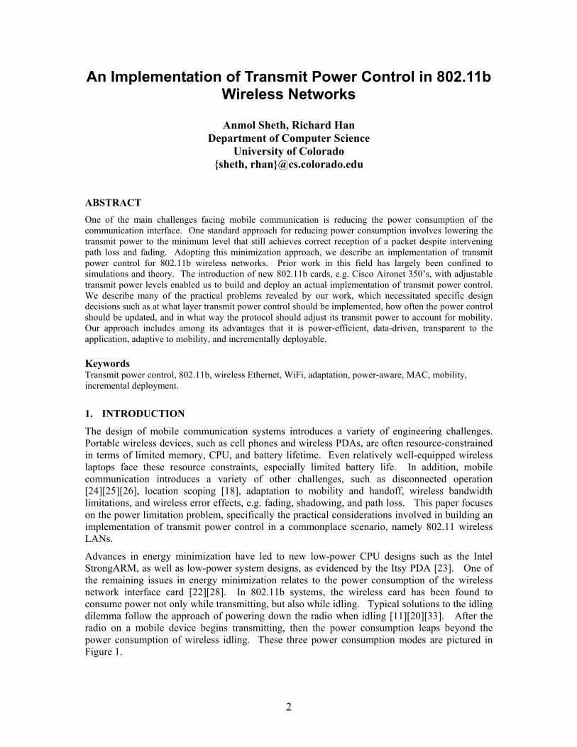
Advances in energy minimization have led to new low-power CPU designs such as the Intel StrongARM, as well as low-power system designs, as evidenced by the Itsy PDA [23]. One of the remaining issues in energy minimization relates to the power consumption of the wireless network interface card [22][28]. In 802.11b systems, the wireless card has been found to consume power not only while transmitting, but also while idling. Typical solutions to the idling dilemma follow the approach of powering down the radio when idling [11][20][33]. After the radio on a mobile device begins transmitting, then the power consumption leaps beyond the power consumption of wireless idling. These three power consumption modes are pictured in Figure 1.

2

In this paper, we focus on the issue of reducing power consumption while the radio is actively transmitting, namely in region C of Figure 1. A standard approach for reducing power consumption due to radio transmission involves lowering the transmit power to the minimum level that still achieves correct reception of a packet despite intervening path loss and fading. Existing research on transmit power control in wireless ad hoc networks [15][16] provides a sound framework from which to consider implementation issues for practical adaptive transmit power control. However, prior work is largely confined to simulations and theory. We provide a more thorough examination of related work on transmit power control in Section 6.

Figure 1: Consumption of a mobile device with and without a wireless network interface.

The primary objective of our work is therefore to design, implement and test a transmit power control algorithm that is able to reduce transmit power consumption in 802.11b LANs to as close to the idle power consumption level as is practical. While power efficiency is our overriding goal, our solution should also satisfy a variety of other design goals. Our approach should be bandwidth-efficient, in that the messaging overhead required to inform the endpoints of a connection as to the optimum transmit power should be minimal. Also, our approach should be adaptive, in case there is motion of nodes. Ideally, we also desire application transparency so that existing applications need not be rewritten in order to take advantage of power control. Another design goal is to allow our solution to be incrementally deployable, so that wireless 802.11 peers can continue to send data to one another if one or the other endpoint has not yet deployed support for transmit power control. Finally, our goal is to design a general transmit power algorithm that is compatible not only with 802.11b, but also with other IR and RF-modulated wireless systems.

In summary, the main design goals of our system are:

• Power-efficiency

• Bandwidth-efficiency

• Adaptation to mobility

• Incremental deployment

• Transparency to application

• Compatibility with 802.11b and other wireless IR/RF standards

3

In the rest of the paper, we first describe the basic algorithm for optimal transmit power control in Section 2. Section 3 explains one of our major design decisions, namely at what layer in the protocol stack to implement transmit power control. This decision had implications on our goals of incremental deployment, transparency to the application, and compatibility across 802.11b and other standards. Section 4 describes how often and in what manner we adjust the transmit power control, thereby addressing our goals of bandwidth efficiency and adaptation to mobility. In Section 5, we describe our experimental setup using the Cisco Aironet 350 wireless PC cards with adjustable transmit power, and analyze the performance of our adaptive transmit power control algorithm in the presence of transmitted TCP traffic as well as mobility. Further related work on transmit power control is discussed in section 6. 2. OPTIMAL TRANSMIT POWER

As discussed in section 1, our basic approach is to modulate the transmit power based on the proximity of the communicating node, to the minimum level such that the destination node still achieves correct reception of a packet despite intervening path loss and fading. In this section, we briefly describe the capabilities of the Cisco Aironet 350 series 802.11b PC cards, and then describe how we determine the optimal transmit power, and finally describe the distributed algorithm that calculates the optimal transmit power.

2.1 Cisco Aironet 350 series

To be able to modulate the transmit power we require discrete power levels which can be set on the network interface. For better savings we require as many power levels as possible. The Cisco Aironet 350 series offers 6 discrete power levels. The table below lists the power levels in dBm and mW. The default transmit power is 20 dBm. In our experiments, we were often able to drive down the optimal transmit power down to 0 dBm and still achieve correct reception of packets while saving 20 dBm – 0 dBm = 99 mW of transmit power.

Table powerthe Ci

The Cisco Aironet 350 series cards acan be extracted on a per-packet bacards, we used the pcmcia-cs-3.1.31for recording the received signal strcall from the driver.

mW dBm 100 20 50 17 30 15 20 13 5 7 1 0

1: Range of transmit settings available on sco Aironet 350 series.

lso have the benefit that the Received Signal Strength (RSSI) sis from the wireless card. For the Cisco Aironet 350 series drivers available for Linux. The drivers have the provision

ength information (RSSI), which can be extracted by an ioctl

4

2.2 Power Loss Model

The basic power loss model that we use is a simplification of the one proposed in [28]. The path loss of a wireless link can be represented by the difference between the transmit power Ptx and receive power Prx.

Path Loss = Ptx – Prx (1)

In this expression, we are grouping a variety of effects, including multipath fading, shadowing, and path loss, under the general term “Path Loss”. This term describes the collective effect of these individual wireless loss mechanisms in reducing the transmitted power down to the received signal strength.

A typical 802.11b PC card will have a power tolerance limit Pthresh below which correct reception of a packet cannot be guaranteed, due to inability of the electronics to extract the signal when the SNR is low. This threshold is the minimum power required to detect a packet off the medium. Hence reducing the transmit power from equation 1 below this threshold would increase the Bit Error Rate (BER) and packets would need to be retransmitted. For our implementation, the 350 cards support a threshold power of –80dBm. Due to the attenuation in the signal from path loss and multipath effects, we calculate the optimal transmit power as:

PTxOpt = Path Loss + Pthresh (2)

In practice, since the lower limit of the transmit power is 0 dBm, PTxOpt is the minimum of 1 mW and equation 2.

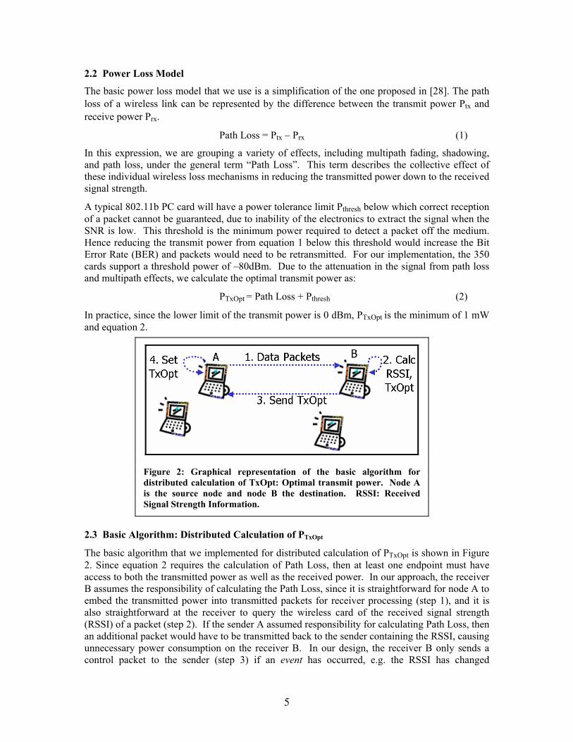
Figure 2: Graphical representation of the basic algorithm for distributed calculation of TxOpt: Optimal transmit power. Node A is the source node and node B the destination. RSSI: Received Signal Strength Information.

2.3 Basic Algorithm: Distributed Calculation of PTxOpt

The basic algorithm that we implemented for distributed calculation of PTxOpt is shown in Figure 2. Since equation 2 requires the calculation of Path Loss, then at least one endpoint must have access to both the transmitted power as well as the received power. In our approach, the receiver B assumes the responsibility of calculating the Path Loss, since it is straightforward for node A to embed the transmitted power into transmitted packets for receiver processing (step 1), and it is also straightforward at the receiver to query the wireless card of the received signal strength (RSSI) of a packet (step 2). If the sender A assumed responsibility for calculating Path Loss, then an additional packet would have to be transmitted back to the sender containing the RSSI, causing unnecessary power consumption on the receiver B. In our design, the receiver B only sends a control packet to the sender (step 3) if an event has occurred, e.g. the RSSI has changed

5

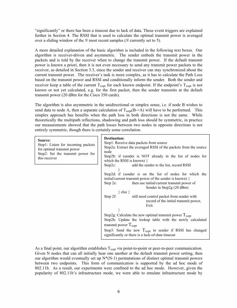
“significantly” or there has been a timeout due to lack of data. These event triggers are explained further in Section 4. The RSSI that is used to calculate the optimal transmit power is averaged over a sliding window of the N most recent samples (N currently set to 5). A more detailed explanation of the basic algorithm is included in the following text boxes. Our algorithm is receiver-driven and asymmetric. The sender embeds the transmit power in the packets and is told by the receiver when to change the transmit power. If the default transmit power is known a priori, then it is not even necessary to send any transmit power packets to the receiver, as detailed in Section 3.3, since the sender and receiver can stay synchronized about the current transmit power. The receiver’s task is more complex, as it has to calculate the Path Loss based on the transmit power and RSSI and conditionally inform the sender. Both the sender and receiver keep a table of the current Txopt for each known endpoint. If the endpoint’s Txopt is not known or not yet calculated, e.g. for the first packet, then the sender transmits at the default transmit power (20 dBm for the Cisco 350 cards). The algorithm is also asymmetric in the unidirectional or simplex sense, i.e. if node B wishes to send data to node A, then a separate calculation of Txopt(B->A) will have to be performed. This simplex approach has benefits when the path loss in both directions is not the same. While theoretically the multipath reflections, shadowing and path loss should be symmetric, in practice our measurements showed that the path losses between two nodes in opposite directions is not entirely symmetric, though there is certainly some correlation.

AGob8p

Source: Step1: Listen for incoming packetsfor optimal transmit power Step2: Set the transmit power forthis receiver

s a final point, our algorithm establishiven N nodes that can all initially heur algorithm would eventually set up etween two endpoints. This form o02.11b. As a result, our experimentsopularity of 802.11b’s infrastructure

Destination: Step1: Receive data packets from source Step2a: Extract the averaged RSSI of the packets from the source node Step2b: if (sender is NOT already in the list of nodes for which the RSSI is known) Step2c: add the sender to the list, record RSSI Step2d: if (sender is on the list of nodes for which the initial/current transmit power of the sender is known) Step 2e: then use initial/current transmit power of

Sender in Step2g (20 dBm) else

Step 2f: still need control packet from sender with record of the initial transmit power, Exit.

Step2g: Calculate the new optimal transmit power Txopt Step2h: Update the lookup table with the newly calculated transmit power Txopt Step3: Send the new Txopt to sender if RSSI has changed significantly or there is a lack-of-data timeout

es Txopt via point-to-point or peer-to-peer communication. ar one another at the default transmit power setting, then N*(N-1) permutations of distinct optimal transmit powers f communication is supported by the ad hoc mode of

were confined to the ad hoc mode. However, given the mode, we were able to emulate infrastructure mode by

6

placing a Network Address Translation (NAT) gateway on an edge node of the ad hoc network, and thereby bridge into the Internet and Web from the ad hoc wireless LAN. We expect that our algorithm is compatible with infrastructure mode and, as part of our future work, do not anticipate significant difficulties in porting our adaptive transmit power control algorithm to infrastructure mode. 3. ARCHITECTURE

Given Section 2’s basic distributed algorithm for calculating the optimal transmit power between two nodes, a clear design issue concerns at what layer in the protocol stack should the sender and receivers communicate to establish the optimal transmit power? The implications of this design choice will affect our design goals of application transparency, incremental deployment, and compatibility. We evaluated 3 different architectures below, and explain our ultimate choice of an application-layer design. 3.1 Shim Layer Approach

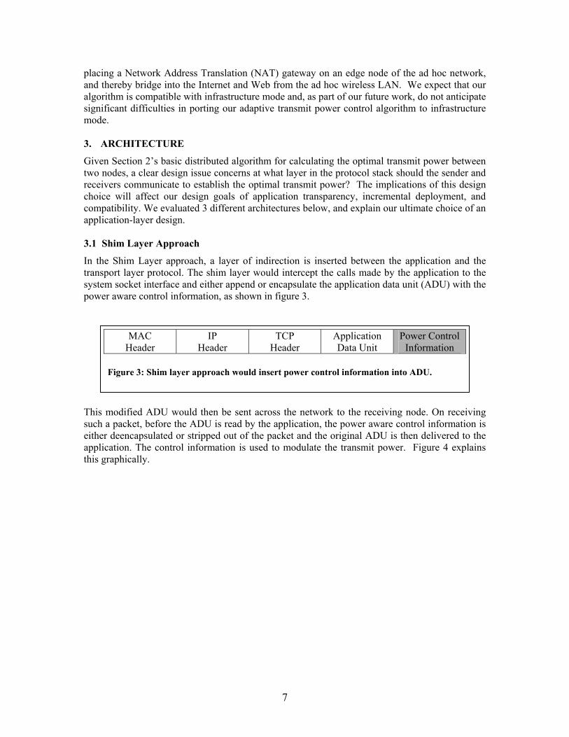
In the Shim Layer approach, a layer of indirection is inserted between the application and the transport layer protocol. The shim layer would intercept the calls made by the application to the system socket interface and either append or encapsulate the application data unit (ADU) with the power aware control information, as shown in figure 3.

Figu

This modsuch a paeither deeapplicatiothis graph

MAC Header

IP Header

TCP Header

Application Data Unit

Power Control Information

re 3: Shim layer approach would insert power control information into ADU.

ified ADU would then be sent across the network to the receiving node. On receiving cket, before the ADU is read by the application, the power aware control information is ncapsulated or stripped out of the packet and the original ADU is then delivered to the n. The control information is used to modulate the transmit power. Figure 4 explains ically.

7

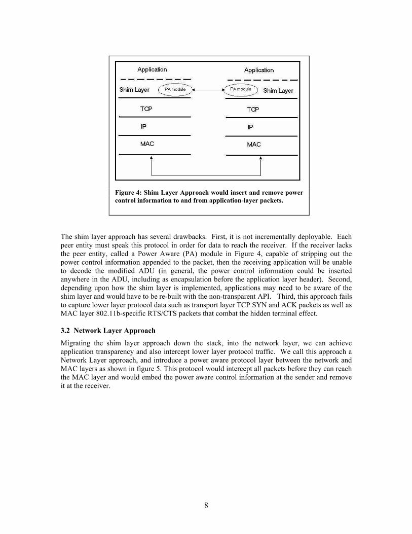
Figure 4: Shim Layer Approach would insert and remove power control information to and from application-layer packets.

The shim layer approach has several drawbacks. First, it is not incrementally deployable. Each peer entity must speak this protocol in order for data to reach the receiver. If the receiver lacks the peer entity, called a Power Aware (PA) module in Figure 4, capable of stripping out the power control information appended to the packet, then the receiving application will be unable to decode the modified ADU (in general, the power control information could be inserted anywhere in the ADU, including as encapsulation before the application layer header). Second, depending upon how the shim layer is implemented, applications may need to be aware of the shim layer and would have to be re-built with the non-transparent API. Third, this approach fails to capture lower layer protocol data such as transport layer TCP SYN and ACK packets as well as MAC layer 802.11b-specific RTS/CTS packets that combat the hidden terminal effect. 3.2 Network Layer Approach

Migrating the shim layer approach down the stack, into the network layer, we can achieve application transparency and also intercept lower layer protocol traffic. We call this approach a Network Layer approach, and introduce a power aware protocol layer between the network and MAC layers as shown in figure 5. This protocol would intercept all packets before they can reach the MAC layer and would embed the power aware control information at the sender and remove it at the receiver.

8

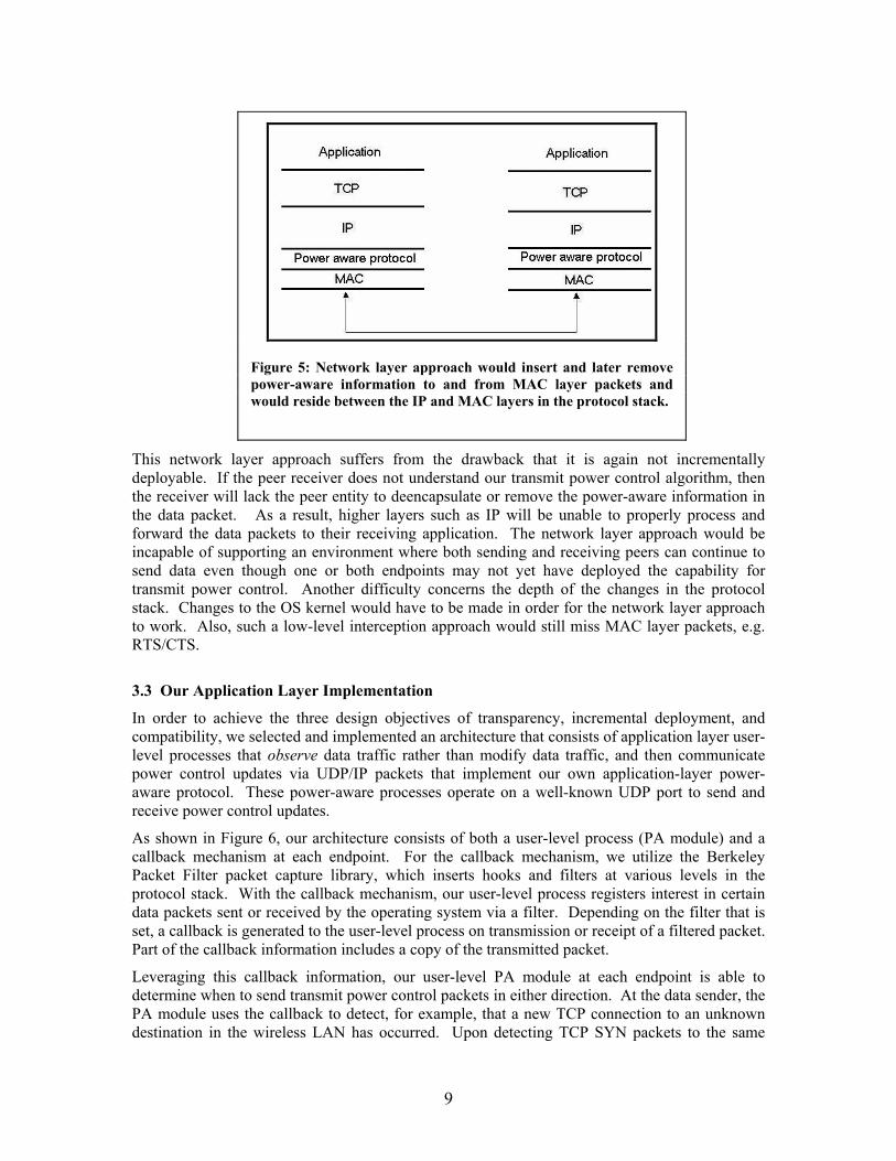
Figure 5: Network layer approach would insert and later remove power-aware information to and from MAC layer packets and would reside between the IP and MAC layers in the protocol stack.

This network layer approach suffers from the drawback that it is again not incrementally deployable. If the peer receiver does not understand our transmit power control algorithm, then the receiver will lack the peer entity to deencapsulate or remove the power-aware information in the data packet. As a result, higher layers such as IP will be unable to properly process and forward the data packets to their receiving application. The network layer approach would be incapable of supporting an environment where both sending and receiving peers can continue to send data even though one or both endpoints may not yet have deployed the capability for transmit power control. Another difficulty concerns the depth of the changes in the protocol stack. Changes to the OS kernel would have to be made in order for the network layer approach to work. Also, such a low-level interception approach would still miss MAC layer packets, e.g. RTS/CTS.

3.3 Our Application Layer Implementation

In order to achieve the three design objectives of transparency, incremental deployment, and compatibility, we selected and implemented an architecture that consists of application layer user-level processes that observe data traffic rather than modify data traffic, and then communicate power control updates via UDP/IP packets that implement our own application-layer power-aware protocol. These power-aware processes operate on a well-known UDP port to send and receive power control updates.

As shown in Figure 6, our architecture consists of both a user-level process (PA module) and a callback mechanism at each endpoint. For the callback mechanism, we utilize the Berkeley Packet Filter packet capture library, which inserts hooks and filters at various levels in the protocol stack. With the callback mechanism, our user-level process registers interest in certain data packets sent or received by the operating system via a filter. Depending on the filter that is set, a callback is generated to the user-level process on transmission or receipt of a filtered packet. Part of the callback information includes a copy of the transmitted packet.

Leveraging this callback information, our user-level PA module at each endpoint is able to determine when to send transmit power control packets in either direction. At the data sender, the PA module uses the callback to detect, for example, that a new TCP connection to an unknown destination in the wireless LAN has occurred. Upon detecting TCP SYN packets to the same

9

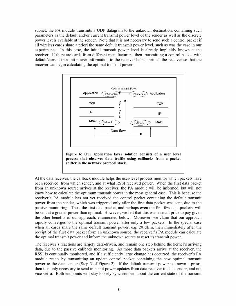
subnet, the PA module transmits a UDP datagram to the unknown destination, containing such parameters as the default and/or current transmit power level of the sender as well as the discrete power levels available at the sender. Note that it is not necessary to send such a control packet if all wireless cards share a priori the same default transmit power level, such as was the case in our experiments. In this case, the initial transmit power level is already implicitly known at the receiver. If there are cards from different manufacturers, then transmitting a control packet with default/current transmit power information to the receiver helps “prime” the receiver so that the receiver can begin calculating the optimal transmit power.

Figure 6: Our applicatiprocess that observes dasniffer in the network pro

w

At the data receiver, the callback module hbeen received, from which sender, and at wfrom an unknown source arrives at the reknow how to calculate the optimum transmreceiver’s PA module has not yet receivepower from the sender, which was triggerepassive monitoring. Thus, the first data pabe sent at a greater power than optimal. Hothe other benefits of our approach, enumerapidly converges to the optimal transmit when all cards share the same default tranreceipt of the first data packet from an unkthe optimal transmit power and inform the

The receiver’s reactions are largely data-drdata, due to the passive callback monitoriRSSI is continually monitored, and if a sufmodule reacts by transmitting an update power to the data sender (Step 3 of Figurethen it is only necessary to send transmit povice versa. Both endpoints will stay loose

Data flo

on layer solution consists of a user level ta traffic using callbacks from a packet

tocol stack.

elps the user-level process monitor which packets have hat RSSI received power. When the first data packet

ceiver, the PA module will be informed, but will not it power in the most general case. This is because the d the control packet containing the default transmit d only after the first data packet was sent, due to the cket, and perhaps even the first few data packets, will wever, we felt that this was a small price to pay given rated below. Moreover, we claim that our approach power after only a few packets. In the special case smit power, e.g. 20 dBm, then immediately after the nown source, the receiver’s PA module can calculate

unknown source to reset its transmit power.

iven, and remain one step behind the kernel’s arriving ng. As more data packets arrive at the receiver, the ficiently large change has occurred, the receiver’s PA control packet containing the new optimal transmit 2). If the default transmit power is known a priori, wer updates from data receiver to data sender, and not

ly synchronized about the current state of the transmit

10

power level. The worst that can happen is if one or more transmit power updates from the data receiver (Step 3) are lost, due to unreliable datagram delivery over wireless links. At this point, both sender and receiver lose synchronization, but the effect is far from catastrophic. Either the sender transmits at too high a power for a short time until the receiver’s updates reach the sender, or the sender transmits at too low a power, in which case the data won’t reach the receiver and the receiver will timeout, prompting a transmit power update (see next section). Eventually, the receiver will be able to communicate with a sender, and communication will be reestablished.

A key advantage of this user-level approach is that it is incrementally deployable. In case one or both endpoints do not speak our transmit power control protocol, then the UDP packets simply are dropped, due to lack of a receiving peer process. Delivery of application data is not affected, except that data will be transmitted at non-optimal power levels. As a result, in an ad-hoc network where some nodes support transmit power adaptation while others do not, data will be exchanged optimally between the nodes with adaptive transmit power capability, while data will continue to be exchanged non-optimally among nodes with fixed transmit power levels.

Another advantage of this application-level approach is that it is inherently transparent to the application. The adjustment of the transmit power occurs outside of the flow of application data. Applications need not be rewritten, and packets need not be modified. Protocol stacks need not be modified except to compile in the existing patches for the BPF packet capture library.

A third advantage of a user-level approach is that such an architecture is compatible with a wide variety of wireless standards including 802.11b. All application-level UDP/IP control packets for updating the transmit power are communicated in-band just like any other datagrams. As a result, this user-level approach could be overlayed upon any wireless IR/RF system with adjustable transmit powers, including 802.11b.

A final advantage is that user-level deployment enables easy experimentation with and rapid upgrade/deployment of new adaptive algorithms.

For completeness, in the event of unreliable delivery of one or more of the datagrams containing the default transmit power, we propose that the sender have a timeout mechanism to resend its default transmit power level, since it will not have seen the first update from the receiver advising the sender to adjust its transmit power. This first update acts as an implicit acknowledgement. We did not implement this feature, since our experiments assumed a uniform default transmit power. 4. ALGORITHMS

While our design goals of transparency, incremental deployment and compatibility were addressed by application-layer design in Section 3.3, this section addresses how we achieve the remaining design goals of bandwidth efficiency and adaptation to mobility. Our twin objectives are to answer the following questions: how can the messaging overhead required to inform the sender to adjust it’s transmit power be minimized?; and how can we detect and react to mobility? Both of these objectives are incorporated into step 3 of our basic algorithm as diagrammed on p. 5, i.e. a message is sent to the sender to update its transmit power only if an event of sufficient magnitude has occurred, either a significant change in the RSSI or a timeout due to lack of data activity. 4.1 Bandwidth Efficiency in Static Ad Hoc Networks

For the moment, let us assume that all nodes are static in an ad hoc 802.11b network, so that we can separately address the first question concerning how to minimize the messaging overhead of transmit power updates. One approach is to update the transmit power once per connection, i.e.

11

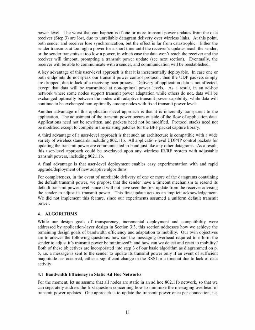
when a TCP SYN packet is received, this will trigger a per-connection one-time-only recalculation of the optimal transmit power. Such an approach would be bandwidth-efficient, but would not react well to changes in RSSI during the course of a TCP connection, as may occur during mobility.

A second approach would involve adjusting the transmit power on a per-packet basis. For each packet received from a given source, the receiver would recalculate the transmit power, and send a control packet to the sender to adjust it’s transmit power. This approach would be bandwidth-inefficient, perhaps even nullifying the saving achieved by transmit power reduction due to the excessive update traffic, but would react most quickly to mobility-induced changes to the RSSI.

Bandwidth

Efficiency Adaptation to Mobility

Per-Connection

(SYN)

YES NO

Per-Packet NO YES Per-Event YES YES

Figure 7: A summary of three classes of adaptation algorithms.

The third approach, which we implemented, was to trigger a recalculation of PTxOpt only when the path loss between the source and destination fall below a predefined trigger level, thus making it an event driven protocol. As explained in section 2 the optimal transmit power is given by the following expression: PTxOpt = Path Loss + Pthresh

However this optimal transmit power i.e. level A in figure 8, is a tight bound and would keep the source and destination just barely connected. Setting the optimal transmit power on this tight bound would result in excessive false triggers, since in a dynamic environment multipath noise can cause fluctuations in the RSSI and nodes can move around (even shifting a laptop by inches can cause destructive interference due to multipath). The frequency of false triggers would overcome the energy savings and also cause interference to the neighboring nodes. As a result, the optimal transmit power should have a cushion above the tight bound. Hence we modify equation (2) to incorporate a cushion. PTxOpt = Path Loss + Pthresh + Mthresh (3)

12

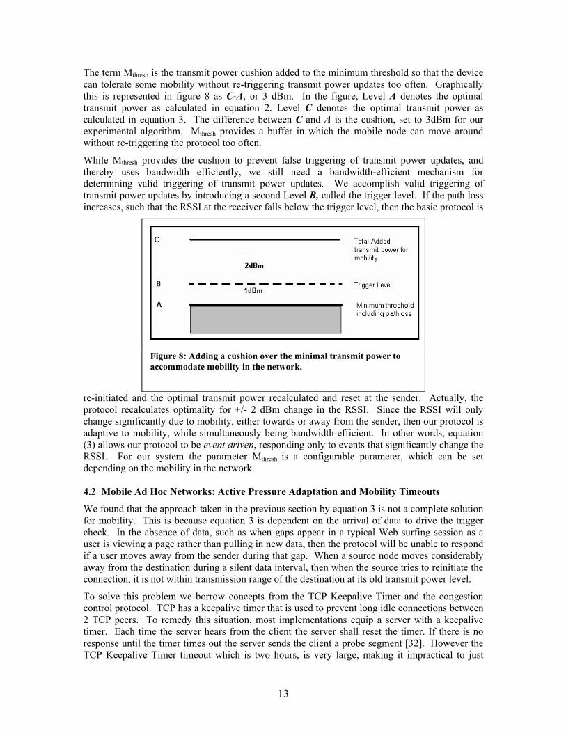
The term Mthresh is the transmit power cushion added to the minimum threshold so that the device can tolerate some mobility without re-triggering transmit power updates too often. Graphically this is represented in figure 8 as C-A, or 3 dBm. In the figure, Level A denotes the optimal transmit power as calculated in equation 2. Level C denotes the optimal transmit power as calculated in equation 3. The difference between C and A is the cushion, set to 3dBm for our experimental algorithm. Mthresh provides a buffer in which the mobile node can move around without re-triggering the protocol too often.

While Mthresh provides the cushion to prevent false triggering of transmit power updates, and thereby uses bandwidth efficiently, we still need a bandwidth-efficient mechanism for determining valid triggering of transmit power updates. We accomplish valid triggering of transmit power updates by introducing a second Level B, called the trigger level. If the path loss increases, such that the RSSI at the receiver falls below the trigger level, then the basic protocol is

re-initiated and the optimal transmit power recalculated and reset at the sender. Actually, the protocol recalculates optimality for +/- 2 dBm change in the RSSI. Since the RSSI will only change significantly due to mobility, either towards or away from the sender, then our protocol is adaptive to mobility, while simultaneously being bandwidth-efficient. In other words, equation (3) allows our protocol to be event driven, responding only to events that significantly change the RSSI. For our system the parameter Mthresh is a configurable parameter, which can be set depending on the mobility in the network.

Figure 8: Adding a cushion over the minimal transmit power to accommodate mobility in the network.

4.2 Mobile Ad Hoc Networks: Active Pressure Adaptation and Mobility Timeouts

We found that the approach taken in the previous section by equation 3 is not a complete solution for mobility. This is because equation 3 is dependent on the arrival of data to drive the trigger check. In the absence of data, such as when gaps appear in a typical Web surfing session as a user is viewing a page rather than pulling in new data, then the protocol will be unable to respond if a user moves away from the sender during that gap. When a source node moves considerably away from the destination during a silent data interval, then when the source tries to reinitiate the connection, it is not within transmission range of the destination at its old transmit power level.

To solve this problem we borrow concepts from the TCP Keepalive Timer and the congestion control protocol. TCP has a keepalive timer that is used to prevent long idle connections between 2 TCP peers. To remedy this situation, most implementations equip a server with a keepalive timer. Each time the server hears from the client the server shall reset the timer. If there is no response until the timer times out the server sends the client a probe segment [32]. However the TCP Keepalive Timer timeout which is two hours, is very large, making it impractical to just

13

depend on the TCP keepalive timer. Hence we borrow TCP’s idea of Keepalive time, by having the timeout as a much smaller time period.

For congestion control TCP has the slow start phase. Initially, TCP sets the congestion window size to 1 and adds one to the congestion window size for each received ACK, assuming no timeouts or duplicate ACKs. This effectively doubles or exponentially increases the number of new packets that can be sent at each roundtrip time. If there is a timeout, the congestion window collapses to one, half the value of the congestion window prior to collapse is saved in the ssthresh variable, and exponential increase continues until ssthresh is reached, followed by additive increase. Thus the acknowledgements that are received for the segments push the window size higher and the loss of segments due to congestion provide active pressure in the reverse direction causing the windows size to reduce.

Combining the 2 strategies we implement the following solution for the problem. We create a timer that times out when the source node has not sent out any data for a pre-defined time period. Once this timer matures, the transmit power is increased by adding another 3dBm as explained in section 4.2. If after another timeout there has still been no data received, then active pressure boosts the transmit power by another 3 dBm. We continue to additively increase the transmit power with each timeout up to the 20 dBm limit (justified below). Thus, if the sender has moved away during a period of inactive data, then this algorithm will attempt to keep the mobile user in contact, by informing the sender to boost its transmit power. When the source node resumes the connection, if the sender has moved away, then it will still be within transmission range with the destination. If the sender has not moved during the inactivity, then the first few packets will be transmitted at an excessive power, whereupon the arriving data will drive the receiver’s PA module to recalculate the optimal transmit power and drive it down to the value of equation 3 again. We therefore expect oscillatory behavior, where active pressure pushes the transmit power up during data inactivity, while data activity drives the transmit power back down to the optimal level. This makes the algorithm data driven.

4.3 Determining Parameter Values

Based on our experimental results, we found that setting Mthresh to a cushion over the minimum threshold power of 3dBm resulted in few false triggers, yet was still low enough to provide for significant power savings. Similarly, we found that setting the trigger level to +/- 2 dBm was sufficient to respond to significant changes in RSSI, while avoiding false positives (there was significant motion though it was not detected) and false negatives (there was no significant motion though an event was triggered). We hope to include these supporting statistical graphs in our next revision.

Using this value of 2 dBm to detect significant mobility, our next objective was to determine the timeout interval. We envisioned a likely indoor scenario where individuals with wireless laptops could communicate with each other and move around during collaboration. We assumed that the average speed of walking for a human being is 1.5m/s. Our question was how far could an individual walk before 2 dBm of RSSI change was noticed at this speed? Table 2 lists the average measured distance as a function of the 802.11b transmit power, taken between two laptops a known measured distance apart. For example, optimal transmit powers of 2-4 dBm corresponded to an average of 9 meters away from the sender, while optimal transmit powers of 4-6 dBm corresponded to an average distance of 10 m away. Therefore, to jump from the 2-4 dBm range to the 4-6 dBm range, a jump of 2 dBm, would correspond to motion of 1 meter, or 2/3 of a second motion at 1.5 m/s. The average of the differences between the distances covered in steps of 2dBm is approximately 10m. Thus, the timeout is roughly 10m/1.5 m/s = 6 seconds.

14

Depending on the mobility involved in the network, we can change the timeout period and hence make the optimal transmit power more resilient to mobility.

Tapr

As part of the justifincreasing the transmhuman walking mobhuman to walk aboulikely, and thereforemobility to/from a no 5. EXPERIMENT This section explaintransmit power. Sec5.2 explains the setanalyze the adaptabifor the transmit poapproach. 5.1 Optimal Transm

To calculate the optdistance. From the rour measurement semeasurements werePCMCIA network icommunicating withreceived signal stretransmit power. Theeffects of multipath(100mW) that the nowas observed that fo

Transmit power in intervals of 2dBm

Distance (m)

Difference (m)

0-2 7 2-4 9 2 4-6 10 1 6-8 21 11

8-10 26 5 10-12 36 10 12-14 46 10 14-16 70 24 16-18 90 20

ble 2: Calculation of the timeout period to re-trigger the otocol for the optimal transmit power

ication for additive increase at 3 dBm per timeout, rather than immediately it power to the maximum of 20dBm, we again considered the scenario of

ility. A conservative jump from say 14dBm to 20dBm would require the t 45 meters (last two rows of Table 2) in 6 seconds. We did not think this only increase the transmit power additively to correspond with linear human de.

AL ANALYSIS

s the measurements we took to calculate the power consumption and optimal tion 5.1 discusses optimal transmit power as a function of distance. Section up and the measured energy consumption at various transmit powers. We lity of our protocol for mobile ad hoc networks in section 5.3. Measurements wer are taken for the event-driven approach as well for the per-packet

it Power

imal transmit power, we measured received signal strength as a function of eceived signal strength, we calculate the path loss. The graphs below show tup as well as a plot of optimal transmit power as a function distance. The taken using 2 laptops each having a Cisco Aironet 350 series wireless nterface configured in ad hoc mode. One laptop was stationary and was the other laptop. The threshold was fixed at -80dBm. We calculated the

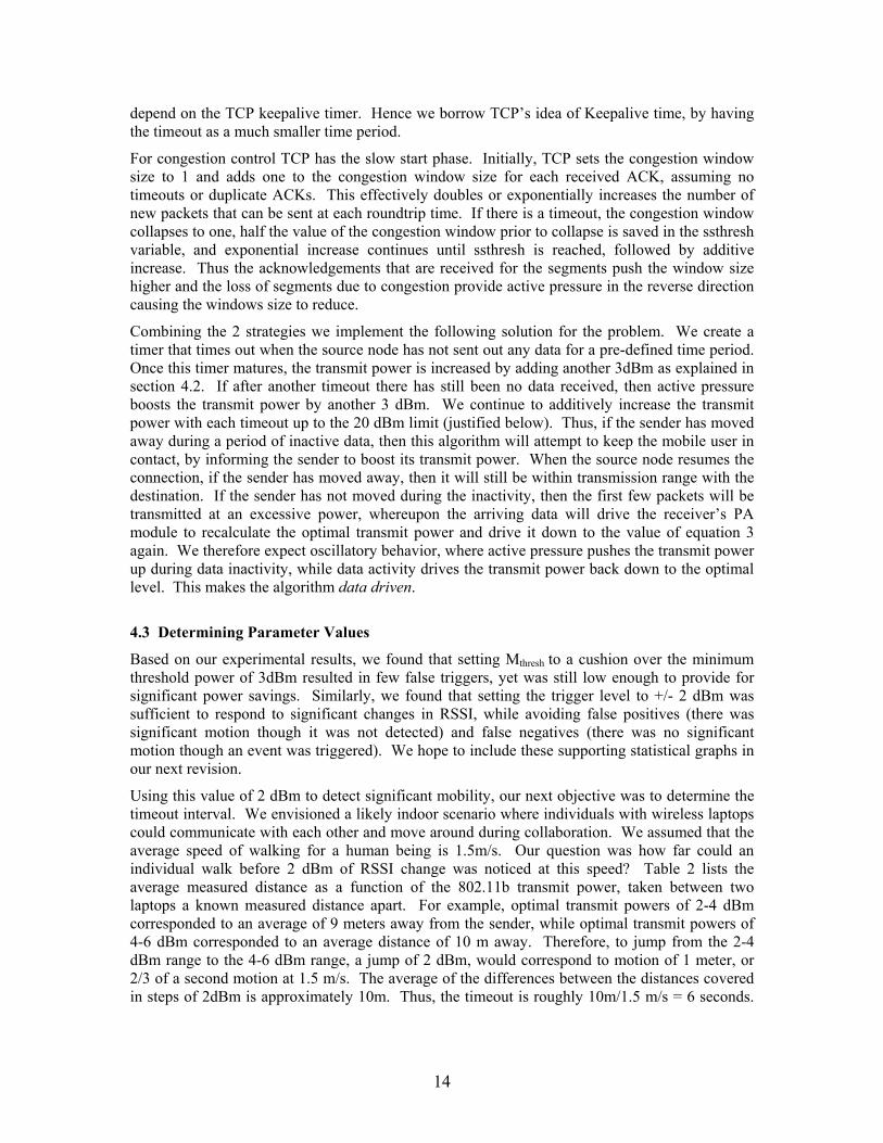
ngth at varying distances and using equation 3 we calculated the optimal received signal strength is averaged over a set of 10 readings to reduce the . The dark line in figure 9 shows the fixed transmit power of 20dBm de would transmit at irrespective of the proximity of the destination node. It r small distances (within range of 5 m.) the optimal transmit power is 0dBm,

15

which is equivalent to 1mW, and therefore a savings of over 99 mW from the default transmit power of 100 mW/20 dBm.

Figure 9: Optimal transmit power as a function of distance. (X-axis scale is not linear)

5.2 Power Consumption

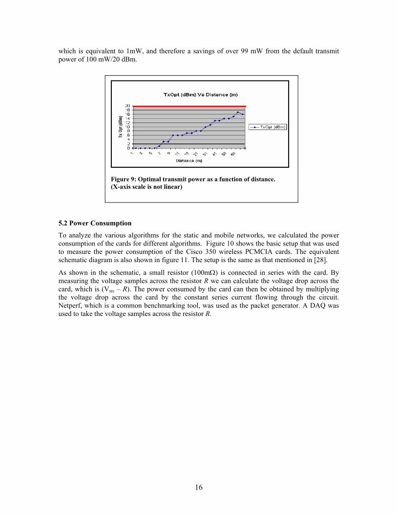
To analyze the various algorithms for the static and mobile networks, we calculated the power consumption of the cards for different algorithms. Figure 10 shows the basic setup that was used to measure the power consumption of the Cisco 350 wireless PCMCIA cards. The equivalent schematic diagram is also shown in figure 11. The setup is the same as that mentioned in [28].

As shown in the schematic, a small resistor (100mΩ) is connected in series with the card. By measuring the voltage samples across the resistor R we can calculate the voltage drop across the card, which is (Vsrc – R). The power consumed by the card can then be obtained by multiplying the voltage drop across the card by the constant series current flowing through the circuit. Netperf, which is a common benchmarking tool, was used as the packet generator. A DAQ was used to take the voltage samples across the resistor R.

16

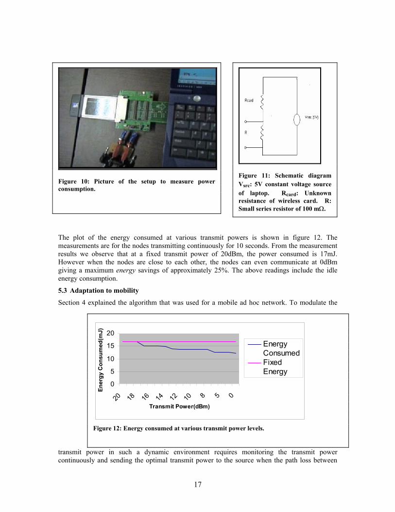
The plot of the energy consumed at various transmit powers is shown in figure 12. The measurements are for the nodes transmitting continuously for 10 seconds. From the measurement results we observe that at a fixed transmit power of 20dBm, the power consumed is 17mJ. However when the nodes are close to each other, the nodes can even communicate at 0dBm giving a maximum energy savings of approximately 25%. The above readings include the idle energy consumption.

5.3 Adaptation to mobility

Section 4 explained the algorithm that was used for a mobile ad hoc network. To modulate the

transmit power in such a dynamic environment requires monitoring the transmit power continuously and sending the optimal transmit power to the source when the path loss between

Figure 11: Schematic diagram Vsrc: 5V constant voltage source of laptop. Rcard: Unknown resistance of wireless card. R: Small series resistor of 100 mΩ.

Figure 10: Picture of the setup to measure power consumption.

Figure 12: Energy consumed at various transmit power levels.

0

5

10

15

20

20 18 16 14 12 10 8 5 0Transmit Power(dBm)

Ener

gy C

onsu

med

(mJ)

EnergyConsumedFixedEnergy

17

the source and destination varies significantly. We illustrate two of the options for resetting the transmit power

• Reset the transmit power for every packet that the destination receives from the source

• Reset the transmit power only when required, as discussed in section 4.2

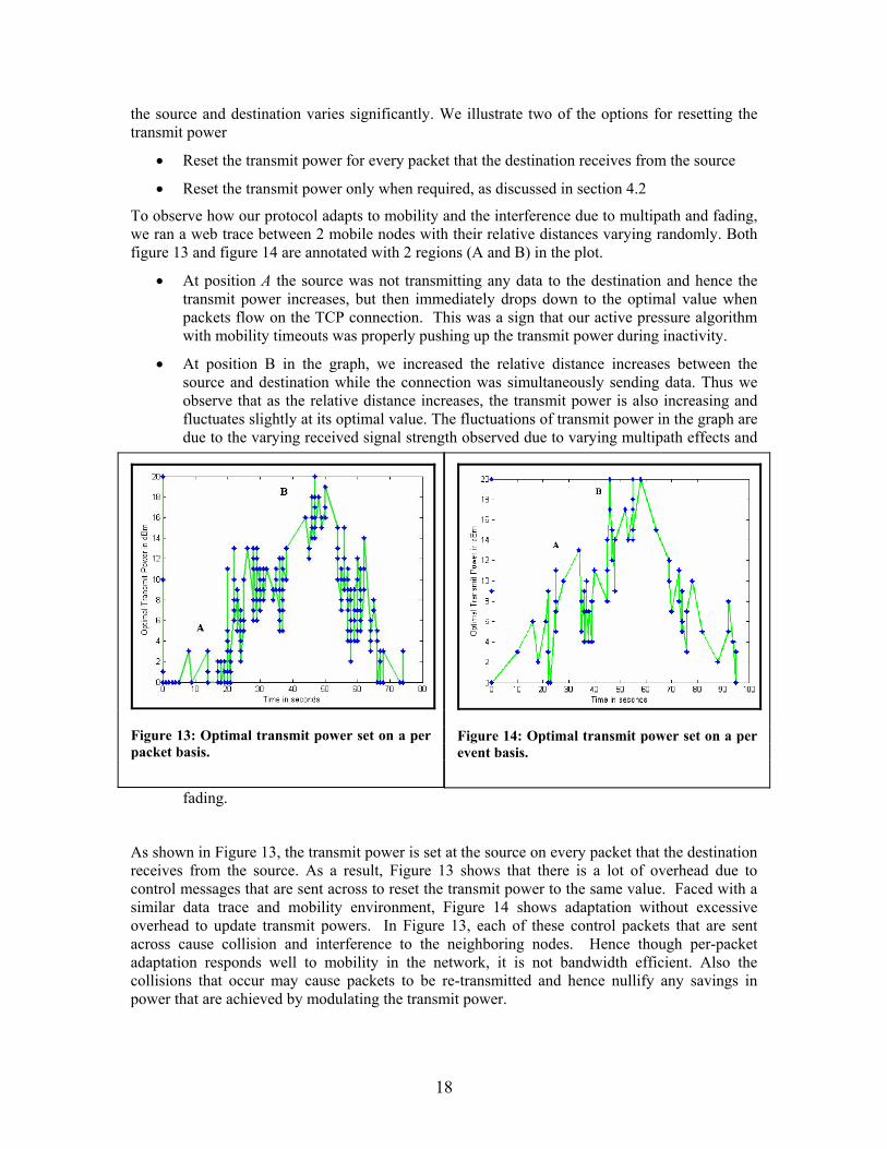
To observe how our protocol adapts to mobility and the interference due to multipath and fading, we ran a web trace between 2 mobile nodes with their relative distances varying randomly. Both figure 13 and figure 14 are annotated with 2 regions (A and B) in the plot.

• At position A the source was not transmitting any data to the destination and hence the transmit power increases, but then immediately drops down to the optimal value when packets flow on the TCP connection. This was a sign that our active pressure algorithm with mobility timeouts was properly pushing up the transmit power during inactivity.

• At position B in the graph, we increased the relative distance increases between the source and destination while the connection was simultaneously sending data. Thus we observe that as the relative distance increases, the transmit power is also increasing and fluctuates slightly at its optimal value. The fluctuations of transmit power in the graph are due to the varying received signal strength observed due to varying multipath effects and

fading.

Figure 14: Optimal transmit power set on a per event basis.

As shown in Figure 13, the transmit power is set at the source on every packet that the destination receives from the source. As a result, Figure 13 shows that there is a lot of overhead due to control messages that are sent across to reset the transmit power to the same value. Faced with a similar data trace and mobility environment, Figure 14 shows adaptation without excessive overhead to update transmit powers. In Figure 13, each of these control packets that are sent across cause collision and interference to the neighboring nodes. Hence though per-packet adaptation responds well to mobility in the network, it is not bandwidth efficient. Also the collisions that occur may cause packets to be re-transmitted and hence nullify any savings in power that are achieved by modulating the transmit power.

Figure 13: Optimal transmit power set on a per packet basis.

18

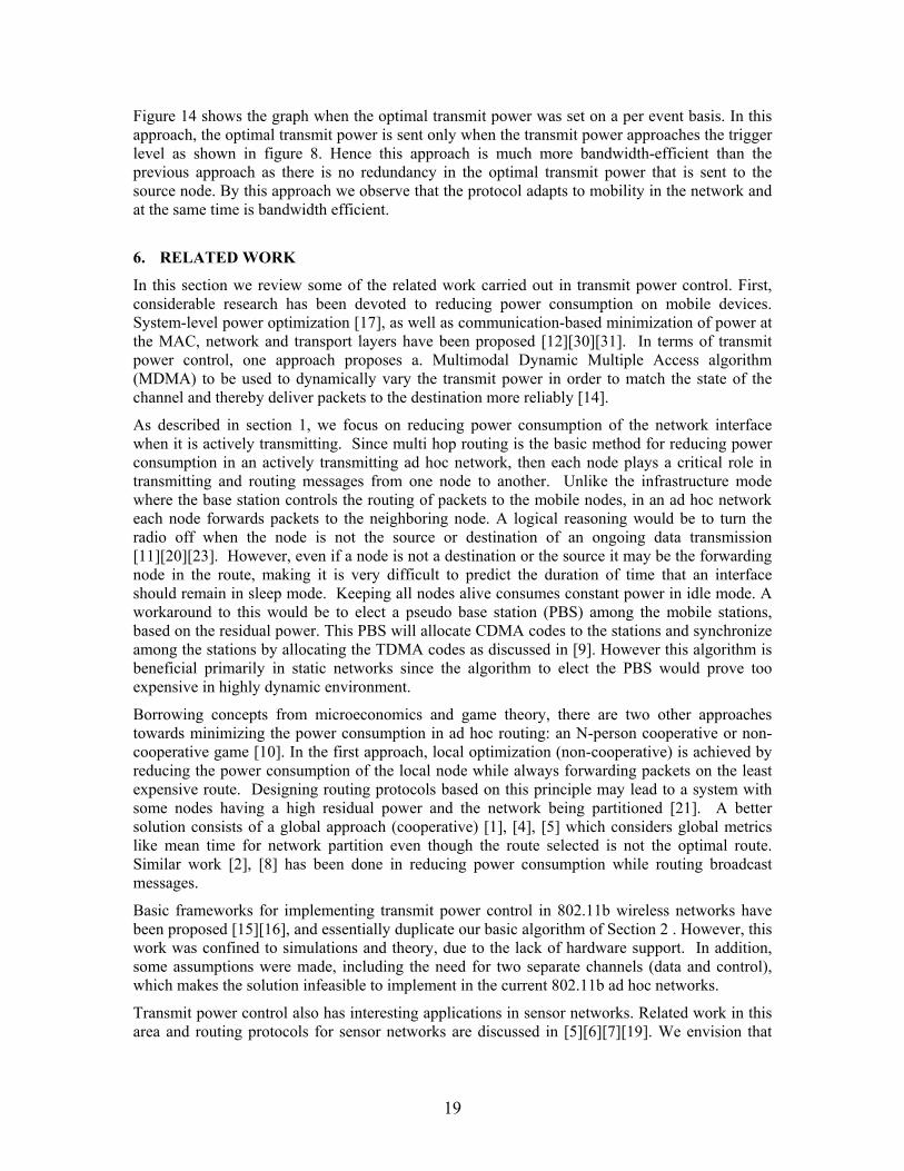
Figure 14 shows the graph when the optimal transmit power was set on a per event basis. In this approach, the optimal transmit power is sent only when the transmit power approaches the trigger level as shown in figure 8. Hence this approach is much more bandwidth-efficient than the previous approach as there is no redundancy in the optimal transmit power that is sent to the source node. By this approach we observe that the protocol adapts to mobility in the network and at the same time is bandwidth efficient. 6. RELATED WORK

In this section we review some of the related work carried out in transmit power control. First, considerable research has been devoted to reducing power consumption on mobile devices. System-level power optimization [17], as well as communication-based minimization of power at the MAC, network and transport layers have been proposed [12][30][31]. In terms of transmit power control, one approach proposes a. Multimodal Dynamic Multiple Access algorithm (MDMA) to be used to dynamically vary the transmit power in order to match the state of the channel and thereby deliver packets to the destination more reliably [14].

As described in section 1, we focus on reducing power consumption of the network interface when it is actively transmitting. Since multi hop routing is the basic method for reducing power consumption in an actively transmitting ad hoc network, then each node plays a critical role in transmitting and routing messages from one node to another. Unlike the infrastructure mode where the base station controls the routing of packets to the mobile nodes, in an ad hoc network each node forwards packets to the neighboring node. A logical reasoning would be to turn the radio off when the node is not the source or destination of an ongoing data transmission [11][20][23]. However, even if a node is not a destination or the source it may be the forwarding node in the route, making it is very difficult to predict the duration of time that an interface should remain in sleep mode. Keeping all nodes alive consumes constant power in idle mode. A workaround to this would be to elect a pseudo base station (PBS) among the mobile stations, based on the residual power. This PBS will allocate CDMA codes to the stations and synchronize among the stations by allocating the TDMA codes as discussed in [9]. However this algorithm is beneficial primarily in static networks since the algorithm to elect the PBS would prove too expensive in highly dynamic environment.

Borrowing concepts from microeconomics and game theory, there are two other approaches towards minimizing the power consumption in ad hoc routing: an N-person cooperative or non-cooperative game [10]. In the first approach, local optimization (non-cooperative) is achieved by reducing the power consumption of the local node while always forwarding packets on the least expensive route. Designing routing protocols based on this principle may lead to a system with some nodes having a high residual power and the network being partitioned [21]. A better solution consists of a global approach (cooperative) [1], [4], [5] which considers global metrics like mean time for network partition even though the route selected is not the optimal route. Similar work [2], [8] has been done in reducing power consumption while routing broadcast messages.

Basic frameworks for implementing transmit power control in 802.11b wireless networks have been proposed [15][16], and essentially duplicate our basic algorithm of Section 2 . However, this work was confined to simulations and theory, due to the lack of hardware support. In addition, some assumptions were made, including the need for two separate channels (data and control), which makes the solution infeasible to implement in the current 802.11b ad hoc networks.

Transmit power control also has interesting applications in sensor networks. Related work in this area and routing protocols for sensor networks are discussed in [5][6][7][19]. We envision that

19

our algorithm can achieve higher savings in IR based sensor networks than 802.11b networks due to the absence of idling power consumption. 7. CONCLUSION This paper presents an implementation of adaptive transmit power control for ad hoc 802.11b wireless networks. Our design goals included power efficiency, bandwidth efficiency, adaptation to mobility, application transparency, incremental deployment, and compatibility with many wireless standards. The basic algorithm consisted of setting the transmit power to the minimum optimal level that still permitted the packets to be received correctly without causing packet loss and retransmissions. One key design choice that achieved transparency, incremental deployment and compatibility was to implement transmit power control as user-level application layer processes. Adaptation to mobility was achieved both by adding a cushion to the optimal transmit power to accommodate minor mobility, as well as adding an adaptive pressure algorithm that boosted the transmit power after a timeout in the absence of data. Bandwidth efficiency was achieved by triggering transmit power updates only after significant change in RSSI. We tested our algorithms for mobility as well as power consumption. Our design decision to re-set the optimal transmit power on a per event basis proved to be more bandwidth-efficient than the naïve approach of resetting the transmit power for every packet, while accomplishing adaptation to mobility. The maximum savings in power that we achieved was 25%, including idling power. 8. REFERENCES [1] Q. Li, J. A. Aslam, D. Rus "Online power-aware routing in wireless Ad-hoc networks" MobiCOm 2001 pp: 97-107. [2] P. Wan, G. Calinescu, X. Li, O. Frieder "Minimum-Energy Broadcast Routing in Static Ad Hoc Wireless Networks" INFOCOM 2001, pp: 1162-1171. [3] R. Ramanathan and R. Rosales-Hain "Topology Control of Multihop Wireless Networks using Transmit Power Adjustment" In Proceedings of IEEE INFOCOM, Tel-Aviv, Israel, March 2000, pp: 404-413. [4] J.-H. Chang and L. Tassiulas, "Energy Conserving Routing in Wireless Ad-hoc Networks," Proc. IEEE INFOCOM 2000, Tel Aviv, Israel, Mar. 2000, pp: 22-31. [5] S. Singh, M. Woo, C.S. Raghavendra "Power-Aware Routing in Mobile Ad Hoc Networks", ACM/IEEE MOBICOM 1998, pp: 181-190. [6] R. C. Shah, J. M. Rabaey "Energy Aware Routing for Low Energy Ad Hoc Sensor Networks", Berkeley Wireless Research Center, University of California, Berkeley [8] F. Li, I. Nikolaidis, "On Minimum-Energy Broadcasting in All-Wireless Networks", In the proceeding of the 26th Annual IEEE Conference on Local Computer Networks (LCN '2001), Nov. 2001, Tampa, Florida, USA [9] Kyu-Tae, Dong-Ho Cho "A MAC Algorithm for Energy-limited Ad-Hoc Networks" Vehicular Technology Conference, 2000. IEEE VTS Fall VTC 2000. 52nd , Volume: 1 , 2000 Page(s): 219 -222 vol.1 [10] M. Xiao, N. B. Shroff, Edwin K. P. Chong "Utility-Based Power Control (UBPC) in Cellular Wireless Systems", INFOCOM 2001: 412-421 [11] M. Papadopouli and H. Schulzrinne. "Effects of power conservation, wireless coverage and cooperation on data dissemination among mobile devices", ACM SIGMOBILE Symposium on Mobile Ad Hoc Networking & Computing (MobiHoc) 2001, October 4-5, 2001, Long Beach, California. [12] G. Girling, J.Li Kam Wa, P. Osborn, R. Stefanova, "The PEN Low Power Protocol Stack" Presented at the 9th IEEE International Conference on Computer Communications and Networks, October 2000, Las Vegas [13] T. Simunic, L. Benini, P. Glynn, and G. De Micheli, "Dynamic Power Management for Portable Systems", MobiCom 2000, pp: 11-19. [14] S. Kandukuri, N. Bambos “Multimodal Dynamic Multiple Access (MDMA) in Power Controlled Wireless Packet Networks.” INFOCOM 2001: 199-208

20

21

[15] J. P. Monks, V. Bharghavan, and Wen-mei Hwu, "A Power Controlled Multiple Access Protocol for Wireless Packet Networks," IEEE INFOCOM 2001, Alaska, April, 2001 pp 219-228 [16] J. P. Monks, V. Bharghavan, and Wen-mei Hwu, "Transmission Power Controlled for Multiple Access Wireless Packet Networks," Proceedings of The 25th Annual IEEE Conference on Local Computer Networks (LCN 2000), Tampa, FL, Nov., 2000 pp 12-21 [17] R. Kravets, K. Schwan, and K. Calvert, "Power Aware Communication for Mobile Computers", Sixth International Workshop on Mobile Multimedia Communication (MoMuC-7), Nov. 1999, vol. 6, pp: 1-10. [18] S. Meguerdichian, F. Koushanfar, M. Potkonjak, M. Srivastava, “Coverage Problems in Wireless Add-Hoc Sensor Networks.” Proceedings of IEEE Infocom, vol. 3, pp. 1380-1387, April 2001. [19] C. Chevallay, R. E. Van Dyck, and T. A. Hall, "Self-organization protocols for wireless sensor networks," Proc. 36th Conf. on Information Sciences and Systems (CISS 2002), Princeton, March 2002. [20] S. Singh and C.S. Raghavendra, “PAMAS: Power aware multi-access protocol with signalling for ad hoc networks,” ACM Computer Communication Review, vol. 28, no. 3, pp. 5–26, July 1998. [21] J. Gomez, A. T. Campbell, M. Naghshineh and C. Bisdikian, "Conserving Transmission Power in Wireless ad hoc Networks", IEEE 9th International Conference on Network Protocols (ICNP'01), Riverside, California. November 11-14 2001. [22] M. Stemm, P. Gauthier, D. Harada, R. H. Katz "Reducing Power Consumption of Network Interfaces in Hand-Held Devices (Extended Abstract)" Proc. 3rd International Workshop on Mobile Multimedia Communications (MoMuc-3), Princeton, NJ, USA, Sept. 1996 vol. 2, pp: 103—112. [23] W. Hamburgen, D. Wallach, M. Viredaz, L.Brakmo, C.Waldspurger,J Barlett, T. Mann, K.Frankas, "Itsy:Stretching the Bounds of Mobile Computing", IEEE Computer, vol 34, no., April 2001,pp. 28-36 [24] J. Kistler, M. Satyanarayanan, "Disconnected Operation in the Coda File System," ACM Transactions on Computer Systems, vol. 10, no. 1, February 1992, pp: 3-25. [25] D. Terry, M. Theimer, K. Petersen, A. Demers, M. Spreitzer, C. Hauser,"Managing Update Conflicts in Bayou, a Weakly Connected Replicated Storage System," Proceedings of the Fifteenth Symposium on Operating Systems Principles," December 1995, pp. 172-182 [26] G. Kueening, G. Popek, "Automated Hoarding for Mobile Computers," ACM SOSP, 1997, pp: 264-275. [27] M. Weiser, B. Welch, A. Demers, S. Shenker, “Scheduling for Reduced CPU Energy", Processdings of the First USENIX Symposium on Operating Systems Design and Implementation, Nov. 1994, pp: 13-23. [28] L. M. Feeney, M. Nilsson "Investigating the energy Consumption of a Wireless Network Interface in an Ad Hoc Networking Environment" IEEE INFOCOM 2001 [29] P. Gupta and P. R. Kumar, "The capacity of wireless networks," IEEE Transactions on Information Theory, vol. IT-46, no. 2, pp. 388-404, March 2000. [30] H. Balakrishnan, S. Seshan, E. Amir, R. H. Katz.“Improving TCP/IP Performance over Wireless Networks”, Proc. 1st ACM Conf. on Mobile Computing and Networking, Berkeley, CA, November 1995. [31] V. Bharghavan, A. Demers, S. Shenker, L. Zhang “MACAW: A media Access Protocol for Wireless LANs” Processing’s of ACM SIGCOMM, 1994 pp. 212-225 [32] B. A. Forouzan “TCP/IP Protocol Suite” McGraw-Hill Publications [33] A. Sinha and A. Chandrakasan, “Dynamic Power Management in Wireless Sensor Networks”, IEEE Design and Test of Computers, March-April 2001, pp. 62-75