Embed Size (px)
Citation preview
Graduate Theses, Dissertations, and Problem Reports
2014
Implementing a Parametric Analysis in the LaModel 3.0 Program Implementing a Parametric Analysis in the LaModel 3.0 Program
Christian Hugo Calderon Arteaga
Follow this and additional works at: https://researchrepository.wvu.edu/etd
Recommended Citation Recommended Citation Calderon Arteaga, Christian Hugo, "Implementing a Parametric Analysis in the LaModel 3.0 Program" (2014). Graduate Theses, Dissertations, and Problem Reports. 5300. https://researchrepository.wvu.edu/etd/5300
This Thesis is protected by copyright and/or related rights. It has been brought to you by the The Research Repository @ WVU with permission from the rights-holder(s). You are free to use this Thesis in any way that is permitted by the copyright and related rights legislation that applies to your use. For other uses you must obtain permission from the rights-holder(s) directly, unless additional rights are indicated by a Creative Commons license in the record and/ or on the work itself. This Thesis has been accepted for inclusion in WVU Graduate Theses, Dissertations, and Problem Reports collection by an authorized administrator of The Research Repository @ WVU. For more information, please contact [email protected].

Implementing a Parametric Analysis in the
LaModel 3.0 Program
Christian Hugo Calderon Arteaga
Thesis submitted to the
Statler College of Engineering and Mineral Resources
at West Virginia University
in partial fulfillment of the requirements for the degree of
Master of Science
in
Mining Engineering
Brijes Mishra, Ph.D., Chair
Felicia Peng, Ph.D.
Yi Luo, Ph.D.
Department of Mining Engineering
Morgantown, West Virginia
2014
Keywords: LaModel, LaMPre, Parametric Analysis, Lamination Thickness.
Copyright 2014 Christian H. Calderon Arteaga
ABSTRACT
Implementing a Parametric Analysis in the LaModel 3.0 Program
Christian H. Calderon Arteaga
This thesis presents a parametric analysis in the LaModel 3.0 software and its corresponding
results by showing how changes to input variables would affect the output of the model.
This analysis was performed by taking of the most important inputs of the model and varying
them inside a predefined range. The result of this variation was studied to determine how
changes on input variables could affect the output of the model. A screening design
technique was used, and it consists in taking the average values of the input variables,
generate a valid range of variation and observe the behavior of the model outputs. The term
“Screening Design” refers to an experimental plan that is intended to find the few significant
factors from a list of several potential ones. The resulting model outputs behavior due to
changes in the input variables is studied as the percentage of the variation between the results
obtained using each of the inputs in the range, and the result obtained using certain reference
input value. The main goal here for a LaModel user is to be able to recognize the percent
variation in the output due to a certain variation in the input.

To my wife Judy, my children Matthew and Christopher.
Thank you for your love!

iv
ACKNOWLEDGEMENTS
I would especially like to thank Dr. Brijes Mishra, my advisor, who helped me through the
final process of my thesis. My sincere thanks must also go to the members of my thesis
committee Dr. Felicia Peng and Dr. Yi Luo. They generously gave their time to offer me
valuable comments toward improving my work. Especially to Dr. Felicia who encouraged
me to walk through the final steps of my thesis.
Special thanks must go to Dr. Keith Heasley, because he gave me the opportunity to research
under his guidance and supervision. I received motivation; encouragement and support from
him during all my graduate studies.
I also want to thank to the Mining Department’s staff, in particular to Karla Vaughan, and
also to all the graduate students from the Mining Department because they gave me their
friendship and support during this years.
I deeply thank my parents, Hermes and Alicia, and my brother Eskander, for their
unconditional support, timely encouragement, and endless patience despite the long distance
between us.
Last but not least, I would like to thank with love to Judy, Matthew and Christopher, my wife
and sons. Judy has been my best friend and great companion, loved, supported, encouraged,
and helped me get through my studies at the WVU.
I believe I would never have completed this work and gotten this far without the support of
these wonderful persons!
v
TABLE OF CONTENTS
ABSTRACT .........................................................................................................................................................II
ACKNOWLEDGEMENTS ............................................................................................................................. IV
TABLE OF CONTENTS ................................................................................................................................... V
TABLE LIST ..................................................................................................................................................... VII
FIGURE LIST ................................................................................................................................................... IX
1 INTRODUCTION ................................................................................................................................... 11
1.1 BACKGROUND ......................................................................................................................................... 11
1.2 STATEMENT OF THE PROBLEM ................................................................................................................ 12
1.3 STATEMENT OF WORK ............................................................................................................................ 13
1.3.1 Methodology. ................................................................................................................................ 14
1.4 SUMMARY OF FOLLOWING CHAPTERS .................................................................................................... 14
2 LITERATURE REVIEW ......................................................................................................................... 15
2.1 BACKGROUND ......................................................................................................................................... 15
2.1.1 LaModel Introduction. .................................................................................................................. 15
2.1.2 Critical Inputs Parameters for LaModel. ..................................................................................... 16
2.1.3 Calibrating the Rock Mass Stiffness. ............................................................................................ 17
2.1.4 Calibrating Gob Stiffness. ............................................................................................................ 26
2.1.5 Calibrating Coal Strength. ........................................................................................................... 32
2.1.6 Calibration’s Implementation in LamPre3.0 ................................................................................ 34
2.2 STUDIES ABOUT LAMODEL. .................................................................................................................... 47
2.3 STUDIES ABOUT LAMODEL PARAMETERS. ............................................................................................. 52
2.4 OTHER SOFTWARE STUDIES. ................................................................................................................... 55
3 METHODOLOGY .................................................................................................................................. 57
3.1 GENERAL DESCRIPTION OF THE METHODOLOGY ................................................................................. 57
3.2 PARAMETER’S DESCRIPTION. ................................................................................................................ 57
3.2.1 La Model’s Input Variables. ......................................................................................................... 57
3.3 PARAMETRIC ANALYSIS DESCRIPTION. ................................................................................................ 65
3.3.1 Lamination Thickness Data Set. ................................................................................................... 65
3.3.2 Coal Strength Data Set. ................................................................................................................ 66
3.3.3 Rock Mass Modulus Data Set. ...................................................................................................... 67
3.3.4 Coal Seam Modulus Data Set. ...................................................................................................... 68
3.3.5 Poisson’s Ratio Data Set. ............................................................................................................. 69
3.3.6 Grid element size Data Set. .......................................................................................................... 70
3.3.7 Surface Effects Data Set. .............................................................................................................. 71
3.4 SUMMARY. ............................................................................................................................................. 71
4 PARAMETRIC ANALYSIS RESULTS ............................................................................................... 72
4.1 PARAMETRIC ANALYSIS ........................................................................................................................ 72
4.1.1 Introduction. ................................................................................................................................. 72
4.1.2 Sensitivity to Lamination Thickness. ............................................................................................. 72
4.1.3 Sensitivity to Coal Strength. ......................................................................................................... 77
4.1.4 Sensitivity to Rock Mass Modulus. ............................................................................................... 83
4.1.5 Sensitivity to Coal Seam Modulus. ............................................................................................... 88
4.1.6 Sensitivity to Poisson’s Ratio. ....................................................................................................... 94
4.1.7 Sensitivity to Grid Element Size. ................................................................................................... 98

vi
4.1.8 Sensitivity to Surface Effects. ...................................................................................................... 102
5 CONCLUSIONS AND FUTURE WORK ......................................................................................... 108
6 REFERENCES ........................................................................................................................................ 117

vii
TABLE LIST
Table 3.1 Base model input parameters. 58
Table 3.2 Input changes on the lamination thickness. 66
Table 3.3 Input changes on the coal strength. 67
Table 3.4 Coal strength and corresponding calibrated values. 67
Table 3.5 Input changes on the rock mass modulus. 67
Table 3.6 Rock mass modulus and corresponding calibrated values. 68
Table 3.7 Input changes on the coal modulus. 68
Table 3.8 Coal modulus and corresponding calibrated values. 69
Table 3.9 Poisson’s Ratio interval of variation. 69
Table 3.10 Poisson’s Ratio and corresponding calibrated values. 70
Table 3.11 Variation of the grid element size. 70
Table 3.12 Use of surface effects relative to the mining depth. 71
Table 4.1 Average and maximum abutment stress variations depending on the lamination
thickness. 74
Table 4.2 Average and maximum convergence variations depending on the lamination
thickness (100 ft as base model). 76
Table 4.3 Effect of the lamination thickness over the pillar safety factor. 77
Table 4.4 Effect of the coal strength on the pillar stress safety factor. 82
Table 4.5 Average and maximum convergence variations depending on the coal seam
modulus. 84
Table 4.6 Average vertical stress and peak abutment stress variations depending on the coal
seam modulus. 86
Table 4.7 Average and maximum convergence variations depending on the coal seam
modulus for calibrated models. 92
Table 4.8 Average vertical stress and peak abutment stress variations depending on the coal
seam modulus for calibrated models. 93
Table 4.9 Pillar safety factor depending on coal seam modulus. 94
Table 4.10 Average vertical stress and peak abutment stress variations depending on the coal
seam modulus for uncalibrated models. 96
Table 4.11 LaModel Running times and iteration number depending on the grid size. 99
Table 4.12 Pillar safety factor depending on the grid size. 99
Table 4.13 Average and maximum convergence variations depending on the grid size. 100
Table 4.14 Average and maximum abutment stress variations depending on the grid size. 102
Table 4.15 LaModel Running times and iteration number depending on the surface effects
feature. 103
Table 4.16 Effect of including the surface effects feature over the pillar safety factor. 103
Table 4.17 Effect of including the surface effects feature over the average vertical stress,
peak stress, average convergence and maximum convergence over the gob (a ‘Y’

viii
indicates using the surface effect, while ‘N’ indicates that surface effects feature was not
used). 105
Table 4.18 Effect of including the surface effects feature over calibrated and uncalibrated
models (a ‘Y’ indicates using the surface effect, while ‘N’ indicates that surface effects
feature was not used). 107
Table 5.1 Input changes on the lamination thickness. 109

ix
FIGURE LIST
Figure 2.1 A comparison of abutment stresses from the field measurements and LaModel
(MSHA, 2008). ............................................................................................................... 19
Figure 2.2 Distribution of abutment stress, showing that 90% of the abutment falls within the
distance of ( H5 ) from the gob edge. (Mark and Chase, 1997). .................................. 21
Figure 2.3 The six material models in LaModel (MSHA, 2008)........................................... 27
Figure 2.4 The critical panel width conceptualization. .......................................................... 28
Figure 2.5 Conceptualization of the abutment angle (Mark, 1990). ...................................... 30
Figure 2.6 New Lamination Thickness Wizard form in LamPre3.0. ..................................... 35
Figure 2.7 New Overburden / Rock Mass Parameters form in LamPre3.0. .......................... 38
Figure 2.8 Wizard for calibrating the Final Modulus of the gob. .......................................... 39
Figure 2.9 Schematic of pillar loading and material code representation.............................. 43
Figure 2.10 Wizard for defining Mark-Bieniawski coal properties. ...................................... 44
Figure 2.11 Setup of periodic topography experiment with LaModel showing the length and
positioning of the extended periodic seam models, (from Whyatt et al, 2011 ) ............. 51
Figure 3.1 Schematic representation of the tutorial #1 second step. ..................................... 60
Figure 4.1 The effect of change the lamination thickness on the abutment stress................. 73
Figure 4.2 The effect of changing the lamination thickness over the convergence. .............. 76
Figure 4.3 The effect of change the coal strength on the convergence.................................. 78
Figure 4.4 The effect of change the coal strength on the abutment stress. ............................ 79
Figure 4.5 The effect of change the coal strength on the pillar stress safety factor. .............. 80
Figure 4.6 The effect of change the coal strength on the convergence for calibrated models.
......................................................................................................................................... 81
Figure 4.7 The effect of change the coal strength on the abutment stress for calibrated
models. ............................................................................................................................ 82
Figure 4.8 The effect of change the rock mass modulus on the convergence (uncalibrated
models). ........................................................................................................................... 83
Figure 4.9 The effect of change the rock mass modulus on the vertical stress (uncalibrated
models). ........................................................................................................................... 85
Figure 4.10 The effect of change the rock mass modulus on the vertical stress (calibrated
models). ........................................................................................................................... 87
Figure 4.11 The effect of change the rock mass modulus on the convergence (calibrated
models). ........................................................................................................................... 88
Figure 4.12 The effect of change the coal seam modulus on the convergence for uncalibrated
models. ............................................................................................................................ 89
Figure 4.13 The effect of change the coal seam modulus on the abutment stress for
uncalibrated models. ....................................................................................................... 90
Figure 4.14 The effect of change the coal seam modulus on the convergence for calibrated
models. ............................................................................................................................ 91

x
Figure 4.15 The effect of change the coal seam modulus on the abutment stress for
calibrated models. ........................................................................................................... 92
Figure 4.16 The effect of changing the Poisson’s Ratio on the convergence over the gob for
uncalibrated models. ....................................................................................................... 95
Figure 4.17 The effect of changing the Poisson’s Ratio on the abutment stress for
uncalibrated models. ....................................................................................................... 96
Figure 4.18 The effect of changing the Poisson’s Ratio on the convergence over the gob for
calibrated models. ........................................................................................................... 97
Figure 4.19 The effect of changing the Poisson’s Ratio on the abutment stress for calibrated
models. ............................................................................................................................ 98
Figure 4.20 The effect of changing the grid element size on the convergence over the gob.
....................................................................................................................................... 100
Figure 4.21 The effect of changing the grid element size on the vertical abutment stress. . 101
Figure 4.22 The effect of include the surface effects feature on the vertical abutment stress.
....................................................................................................................................... 104
Figure 4.23 The effect of include the surface effects feature on the convergence. ............. 105
11
1 INTRODUCTION
1.1 Background
The LaModel program has been used successfully in the U.S. for designing pillars for many
years. Some years ago, the need for a revision of the current analysis tools was evident due
to the Crandall Canyon collapse. After extensive field verification, a calibration procedure
was implemented in la model, where techniques for calibrating the critical input parameters
based on empirical abutment loading, and pillar strength were developed, and verified
(Heasley, 2008 and Heasley et al, 2010). If the behavior of a system is governed by a
mathematical model then a particular behavior is determined by the parameter’s values, so
changes on such parameters will cause alterations in the model’s output behavior. Therefore,
the accuracy of a LaModel analysis depends entirely on the accuracy of the input parameters.
And, for a realistic analysis, the input parameters need to be calibrated with the best available
information, either: measured, observed, empirically or numerically derived (Heasley, 2008).
The calibration procedure developed by Heasley in 2008 guides the user in selecting the
optimum input parameters and to produce a standard model that fits within the verification
database (Heasley and Tulu, 2011). The suggested calibration method produces fairly rigid
specified values of the critical input parameters (Heasley and Tulu, 2011), however, the
method itself does not explain how slight changes on the input variables can affect the
behavior of the LaModel output.
A technique used to measure how much the results of a model are affected by variations in
the values of the input parameters is called parametric analysis. In order to specifically
calibrate the model to the unique conditions at a specific mine, the LaModel user often have

12
to go out of bounds of the suggested calibration. Therefore, a study that shows how
variations on the LaModel input parameters affect the model results is presented in this
document.
1.2 Statement of the Problem
There are several mathematical techniques available to perform mine stability analysis.
Heasley (Heasley, 1998) described the following techniques: finite elements, boundary
element, discrete element, finite difference techniques and hybrid combinations of the
aforementioned techniques. The volume element approach is used by finite element and
finite difference software, for example FLAC3D (Itasca Consulting Group, Inc., 2007). They
can run three-dimensional models but they are usually limited to a single panel because of
computer’s memory limitations. The boundary element approach reduces the complexity of
computational problems to manageable levels by effectively decreasing the dimensions of a
problem (Larson and Whyatt, 2009). In the displacement discontinuity variation of the
boundary–element method, this is accomplished by modeling the coal seam as a crack, or slit,
in an infinite elastic body (Heasley, 1998; Sinha, 1979 and Zipf, 1992a and 1992b).
There are many parameters that play an important role in the underground mine design, such
as the topography, geology, depth, and others. Some analyses as to which are the most
important variables has been done by different authors (Ozbay and Rozgonyi, 2003; Larson
and Whyatt, 2009; Heasley, 2008; Heasley and Tulu, 2011), and generally, empirical data is
used to determine those variables which are difficult to obtain from field data. During the
design phase it is necessary to know in advance the stresses to which the underground
structure will be subject. At this stage, and as stated before, some parameter’s values are
empirically selected or inferred; while some other comes from field sampling and generally

13
are averages of the measured values, therefore, it is necessary to know how the variation of
these parameters could affect the model’s results, and thus the behavior of the underground
structure.
LaModel, a boundary-element program was one of the analysis tools used in the original
design of the mine plan at Crandall Canyon. In the last few years, a standard method of
calibrating LaModel has been developed (Heasley, 2008), and in 2010, that calibration
method was verified, by using 47 deep cover pillar retreat case studies from 11 different
mines (Heasley et al., 2010). The recommended calibration method for LaModel produces
good results (Heasley and Tulu, 2011), but the rigid parameter specification from the
LaModel calibration method interferes with the model flexibility needed for specific
calibration to the unique conditions at a given mine site.
In 2002, a LaModel sensitivity analysis was performed by Roberts et al., they found that
LaModel is better suited to modelling irregular geometries, as the pillar loads are so close to
tributary area theory, but that analysis was performed before to the collapse of the Crandall
Canyon mine, and even before recent improvements to LaModel program and the launch of
LaModel 3.0 were done in 2010. More recently, in 2011, Heasley and Tulu, and also Whyatt
et al., published LaModel sensitivity analyses, but these two works were performed only to a
few important LaModel input variables. Therefore, an extended LaModel parametric
analysis is needed in order to establish the necessary model flexibility to accurately modeling
a specific mining situation.
1.3 Statement of Work
In this report, parametric analyses are performed with a number of input parameters in
LaModel program. These parameters include: the Poisson’s Ratio, grid element size, surface

14
effects, lamination thickness, coal strength, rock mass modulus and coal modulus. By doing
this research effort, potential LaModel users will be able to leverage the present modern
capabilities (coal wizard, gob wizard, strain-softening wizard, lamination thickness wizard,
energy release rate, etc) of the LaModel program to quickly and accurately estimate the
desired mining parameters.
1.3.1 Methodology.
Parametric analysis results for LaModel are presented in this work. A generalized hypothetic
set of input parameters was selected to study the influence of their individual variations on
the output’s model’s behavior. This methodology is valid for the LaModel software but it
could also be applied to other programs. It is also limited to investigate the behavior of the
LaModel’s output due to changes on its input variables, by studying only one inputs variable
at time. . The behavior due to changes on multiple variables and their interactions is beyond
the scope of this research.
1.4 Summary of Following Chapters
First, a literature review and the necessary background theory are developed in Chapter 2.
The methodology that is used is presented on the Chapter 3 and also there is a brief
description of the variables and the methodology for the calculations. The Chapter 4 presents
the results, and the corresponding analysis of the model’s output variables. Finally, the
conclusions are presented on Chapter 5.

15
2 LITERATURE REVIEW
2.1 Background
2.1.1 LaModel Introduction.
The LaModel software is used to model the stresses and displacements on thin tabular
deposits such as coal seams. It uses the displacement/discontinuity variation of the boundary
element method (Heasley, 1998). This innovative boundary element program uses a
laminated overburden model as opposed to a traditional homogeneous elastic overburden
model (Hardy and Heasley, 2006). This laminated overburden gives the model a very
realistic flexibility for stratified sedimentary geologies and multiple-seam mines. Using
LaModel, the total vertical stresses and displacements in the coal seam are calculated, and
also, the individual effects of multiple-seam stress interactions and topographic relief can be
separated and analyzed individually. LaModel can also calculate element safety factors,
pillar safety factors, intra-seam subsidence, energy values, and roof and floor bending
stresses. LaModel can analyze up to 4 multiple seams with complex geometries and variable
topography (Heasley, 2008). Since LaModel’s original introduction in 1996, it has
continually been upgraded (based on user requests) and modernized as operating systems and
programming languages have changed. The present LaModel is written in Microsoft Visual
C++ and runs in the MS Windows operating system. LaModel uses a forms-based system
for inputting model parameters, a spreadsheet-type interface for creating the mine grid and a
graphical post-processor for analyzing the output. It can analyze a 2000 x 2000 grid with 6
different material models and 52 different individual in-seam materials. Recently, the

16
LaModel program has been interfaced with AutoCAD and can take an AutoCAD map of the
pillar plan and overburden, and automatically convert these into the appropriate seam and
overburden grids. Also, the output from LaModel can be downloaded into AutoCAD and
overlaid on the mine map for enhanced analysis and graphical display (Heasley, 2008).
2.1.2 Critical Inputs Parameters for LaModel.
Heasley (2008), said that in order to obtain accurate results using LaModel, and therefore get
an accurate representation of a specific model, as with any other mathematical model, it is
necessary to perform a calibration and validation of the critical input parameters. Generally
the LaModel user is calibrating for accurate stress, loads and pillar safety factors. In a typical
mining situation, the geometry of the mining in the seams and the topography are fairly well
known and accurately discretized into LaModel, but other input parameters must be
calibrated with regard to accurately calculating stresses and loads and therefore pillar
stability and safety factors. According to Heasley (2008) the most critical input parameters
for accurate stress/load calibration have been identified as:
a) The Rock Mass Stiffness
b) The Gob Stiffness
c) The Coal Strength
Using this sequence of parameter calibration, the calibrated value of the subsequent
parameters is determined by the calibrated value of the previous parameters, and changing
the value of any of the preceding parameters will require re-calibration of the subsequent
parameters (MSHA, 2008). The calibration derivation and the recommended strategy of
calibration are discussed in more detail below

17
2.1.3 Calibrating the Rock Mass Stiffness.
The stiffness of the rock mass in LaModel is mainly determined by two parameters, the rock
mass modulus and the rock mass lamination thickness (Heasley 2008). An increase in one of
these two parameters will result in an increase of the stiffness of the overburden and
consequently, the extent of the abutment stresses will increase, the convergence and stress
over the gob areas will decrease and the multiple seam stress concentrations will be
smoothed over a larger area.
2.1.3.1 Rock Mass Modulus.
Heasley (2008) suggests that when calibrating for good stress output, it is recommendable
that the rock mass stiffness be calibrated to produce a reasonable extent of abutment zone at
the edge of the critical gob areas. When calibrating the rock mass stiffness, Heasley found it
to be most efficient to keep constant a selected rock mass modulus and then calibrate the
lamination thickness. It is recommended to determine the average rock mass modulus as a
thickness weighted average of the elastic modulus of the overburden layers (Karabin and
Evanto, 1999), or simply use the default rock mass modulus in LaModel. Since the
lamination thickness will be adjusted as needed with regard to the elastic modulus to
ultimately match the desired extent of the abutment zone as described below, the choice of
rock mass elastic modulus is not very critical to the final objective (except in a multiple-seam
situation).

18
2.1.3.2 Rock Mass Lamination Thickness.
Heasley (2008) suggests to use specific field measurements of the abutment zone from the
given mine, for calibrating the lamination thickness for a model, based on the extent of the
abutment zone. However, often these field measurements are not available. In this case,
visual observations of the extent of the abutment zone could be used. Most operations
personnel in a mine have a good idea of how far the stress effects can be seen from an
adjacent gob. These visual observations can be used to calibrate the lamination thicknesss.
However, with no better information, historical field measurements would indicate that, on
average, the extent of the abutment zone (D) at depth (H) should be (Peng, 2006):
H9.3 D = 2.1
or that 90% of the abutment load (D.9) should be within (Mark and Chase, 1997):
H5D.9 = 2.2
Once the desired extent of the abutment zone has been determined, the lamination thickness
that will match that abutment extent for that particular site can be calculated. In the original
development of LaModel (Heasley, 1998), an equation (equation 4.25) was developed which
gives the abutment stress magnitude (σl) for the laminated overburden model as a function of
the distance (x) from the panel rib (see Figure 2.1):
xh λ E
E 2
e h λ E
E 2
2
P q(x)σ
s
sl
−= 2.3
where:
q = the in-situ stress

19
P = the width of the panel
Es = the elastic modulus of the seam
E = the elastic modulus of the overburden
λ = a parameter of the laminated model
h = the seam thickness
Figure 2.1 A comparison of abutment stresses from the field measurements and
LaModel (MSHA, 2008).
In equation2.3, the in-situ stress (q) is determined as:
H γq = 2.4
where:
γ = the overburden density
H = the seam depth
and

20
( )2υ1 12
tλ
−=
2.5
where:
t = the lamination thickness in the rock mass
υ = Poisson’s Ratio of the rock mass
In the derivation of equation 2.3, it was assumed that the panel is open with no gob loading;
therefore, the total abutment load is the full weight of the overburden for one half of the
panel (qP/2). Also, the equation 2.3 assumes the coal seam is perfectly elastic and there is no
yield zone at the rib of the panel (Heasley, 1998).
The empirically determined distribution of the abutment stress (σa) within the abutment zone
given the extent of the abutment stress (D) as determined in equation 2.1, has been found to
be (Mark, 1992) (see Figure 2.1):
( )2xDD
3L(x)σ
3
sa −=
2.6
where:
Ls = the total side abutment load
From the stress distribution given by equation 2.6, it can be derived that essentially 90% of
the abutment load falls within the distance (D.9) from the edge of the panel, given by the
equation 2.2 (Mark and Chase, 1997) (See figure 2.2).

21
Figure 2.2 Distribution of abutment stress, showing that 90% of the abutment falls within the
distance of ( H5 ) from the gob edge. (Mark and Chase, 1997).
In order to determine the distance from the panel edge which contains a given percentage (n)
of the side abutment load for the laminated overburden model, first, the load needs to be
determined by integrating equation 2.3 over the distance, x, as follows:
∫−
= x
h λ E
E 2
e2
P-qdx (x)σ
s
l 2.7
Then the fraction (n) of the total side abutment load (qP/2) which is contained in a given
distance (Dn) can be determined as (Heasley, 2008):
2
Pq
D h λ E
E 2
e 2
P-q
0 h λ E
E 2
e 2
P-q
D h λ E
E 2
e 2
P-q
(x)σ2
Pnq
ns
sn
s
D
0
l
n
+−
=
−−
−=
= ∫
2.8

22
Simplifying by dividing through by the total abutment load (qP/2) gives:
1D
h λ E
E 2
e -nn
s
+−
= 2.9
Solving for the abutment distance (Dn) for the given percent load (n) and substituting back in
for λ, we get (Heasley, 2008):
( )
( )
( )( )2
s
n
s
n
ns
ns
υ1 12E 2
h t En-1lnD
E 2
h λ En-1lnD
D h λ E
E 2 n-1ln
D h λ E
E 2
e n-1
−−=
−=
−=
−=
2.10
In the last equation (2.10), the extent of the abutment load is directly proportional to the
square root of the rock mass modulus, seam thickness and lamination thickness and inversely
proportional to the square root of the seam modulus.
Solving the equation 2.10 for the lamination thickness (t), and given the extent of the
abutment load, the rock and the seam properties, we have (Heasley, 2008):
( ) ( )
( ) ( )( )
( )
2
n
2
s
2
s
2
n
2
s
n
n-1ln
D
h E
υ1 12E 2t
υ1 12E 2
h t E
n-1ln
D
υ1 12E 2
h t E
n-1ln
D
−=
−=
−=
−
2.11
Then, the lamination thickness (t) required to match a given abutment extent (Dn) is
proportional to the square of the abutment extent, linearly proportional to the seam modulus

23
and inversely proportional to the rock mass modulus and seam thickness. A comparison of
the empirical abutment stress and the matching laminated model abutment stress as
calculated by equation 2.11 is shown in Figure 2.1.
The original derivation of equation 2.3 assumes the seam as linear elastic, but normally this
is not the case and there is some distance (d) of coal yielding at the edge of the panel. On the
other hand, in equations 2.1 and 2.6 the distance of the yielding zone is naturally included by
the field measurements used to determine the extent of the abutment stress. Therefore, to use
an abutment extent measured in the field as input to equation 2.11, and in order to be
consistent with the derivation of that equation, the extent of the actual yield zone in the field
needs to be subtracted from the field measurement (This adjustment essentially neglects the
amount of overburden load carried in the yield zone.) After making this yield zone
adjustment to the extent of the abutment zone and substituting the equation 2.2 for the
distance of 90% load, the equation of the lamination thickness (t) required to match the field
measurements is as follows (Heasley, 2008):
( )( )
22
s
0.1ln
dH5
h E
υ1 12E 2t
−−= 2.12
where:
E = the elastic modulus of the overburden
υ = the Poisson’s Ratio of the overburden
Es = the elastic modulus of the seam
h = the seam thickness
d = the extent of the coal yielding at the edge of the gob

24
H = the seam depth
2.1.3.3 Yield Zone Distance.
The extent of the yield zone is the only parameter in the equation 2.12 that is not necessarily
known ahead of time. It can be found by running LaModel and observing the calculated
yield zone for the given conditions. Or, to get a first approximation of the yield zone extent,
one can find the point (x) into the pillar rib where the total load carrying capability of the
coal rib is equal to the load distributed by the side abutment. First, to determine the load
carrying capability of the coal rib, we start with the stress gradient implied by the Mark-
Bieniawski coal strength formula (Mark, 1999):
+=
h
x 2.16 0.64S(x) ipσ 2.13
where:
σp(x) = peak coal stress (psi)
x = distance into the coal rib
Si = in-situ coal strength (psi)
h = pillar height
Integrating the last equation with respect to x and evaluating from the rib (x=0) to the
distance x into the pillar, the total load carried by the edge of the pillar rib can be determined
by:
∫ += x0.64 x
h
1.08Sdx (x)σ
2
i
x
0p 2.14

25
The load distributed by the side abutment within the distance x for the laminated overburden
model was previously determined in equation 2.8. If these two loads are set equal, the
following equation is determined (Heasley, 2008):
0xS 0.64xh
S1.08
2
Pq
xh λ E
E 2
e 2
P q- i
2i
s
=−−+−
2.15
In equation 2.8, it was assumed that there was no gob and the total overburden load over half
of the panel became the total abutment load. In the general case, the gob is supporting some
percentage of the overburden load and the remainder of the overburden load becomes
abutment load. If the percentage of the total overburden load over the gob that becomes
abutment load at the edge of the panel is (m), then equation 2.15 can be written as (Heasley,
2008):
0xS 0.64xh
S1.08
2
Pq m
xh λ E
E 2
e 2
P q m- i
2i
s
=−−+−
2.16
Therefore, the value of x which solves equation 2.15 is the point where the cumulative load
carrying capability of the pillar rib equates to the load distributed by the abutment stress
gradient. This is the point in Figure 2.3 where the loading curves cross and this value is a
good first estimate of the depth of the yield zone (d). Equation 2.16 is obviously non-linear
and cannot be solved analytically; however, a numerical value can easily be determined by
means of a numeric solution.
So, for determining the rock mass stiffness to use in LaModel, it is recommended to:

26
a) Determine the average rock mass modulus as a thickness weighted average of the
elastic modulus of the overburden layers, or to use the default rock mass modulus in
LaModel.
b) Then, determine the lamination thickness that matches the observed behavior
(equation 2.11) or average field measurements (equation 2.13)
c) For estimating the depth of the yield zone at the coal rib of the abutment, use
observations from the field or use equation 2.16
2.1.4 Calibrating Gob Stiffness.
In a LaModel analysis with gob areas, an accurate stiffness for the gob (in relation to the
stiffness of the rock) is critical to accurately calculating the overburden load distribution and
therefore the pillar stresses and safety factors. Hence the gob stiffness should be calibrated
using the best available information on the amount of abutment load (or gob load)
experienced at the mine. Therefore, the primary option is to use site specific field
measurements of the abutment load (or gob load), in order to calibrate the gob stiffness.
However, these types of field measurements are quite rare, and often of questionable
accuracy; while visual observations are not very useful for estimating abutment loads or gob
loads, and hence, general historical measurements and/or empirical information are quite
often the only available data.
In LaModel, the stiffness of the gob is primarily determined by adjusting the “Final
Modulus” of the strain-hardening gob model (Heasley 1998) (see Figure 2.3). A higher final
modulus gives a stiffer gob and a lower modulus value produces a softer gob material.

27
Figure 2.3 The six material models in LaModel (MSHA, 2008).
2.1.4.1 Critical Gob Width.
In order to calibrate the gob stiffness for a given situation, there are a number of general
guiding factors to consider. First, a comparison of the present gob width with the critical gob
width for the given depth can provide some useful insight. The critical gob width (Pc) for a
given gob depth (H) and abutment angle (β) can be calculated as:
) β tan(H 2Pc = 2.17
where:
Pc = critical gob width
H = depth
β = abutment angle

28
Figure 2.4 The critical panel width conceptualization.
For a critical (or supercritical) panel width (where the maximum amount of subsidence has
been achieved) (see figure 2.4), it would be expected that the peak gob load in the middle of
the panel would approach the in-situ overburden load. As the depth increases and the gob
width becomes more subcritical, it is expected that the peak gob load would similarly
decrease from the in-situ load. As a first approximation, the peak stress on the longwall gob
can be expected to be around the same percentage of the in-situ stress as the gob width is a
percentage of the critical gob width.
2.1.4.2 Laminated Model Gob Stress.
With increasing depth from the critical situation, the gob width becomes more subcritical, a
laminated overburden analysis with a linear elastic gob material would suggest that the peak
gob load would increase linearly with depth from the load level in the critical case (Chase et
al., 2002; Heasley, 2000). The critical depth (Hc) for a given gob width (P) and abutment
angle (β) can be calculated as (Heasley 2008):
) β tan(2
PHc
×= 2.18
β
β β
Super-Critical Sub-Critical

29
where:
Hc = Critical Depth
P = Panel Width
β = Abutment Angle
For the actual seam depth (H) (greater than Hc), the expected average gob stress based on the
laminated model (σgob-lam-av) is given by (MSHA, 2008):
×=
×
×
=−
288
γH
1442
γH
H
Hσ c
c
avlam-gob 2.19
where:
H = Seam Depth (ft)
γ = Overburden Density (lbs/cu ft)
The laminated overburden and a linear elastic gob in equation 2.19 imply that the average
gob stress for a subcritical panel is solely a function of the depth and equal to half of the in-
situ stress. (Generally, the gob material is considered to be strain-hardening and therefore,
equation 2.19 may underestimate the actual gob loading (MSHA, 2008).)
2.1.4.3 Abutment Angle Gob Stress.
For estimating the gob and abutment loading in ALPS and ARMPS, an average abutment
angle of 21º was determined from an empirical database (Mark, 1992 and Mark and Chase,
1997). Using the abutment angle concept, the average gob stresses (σg-av) for a supercritical
panel (see Figure 2.5) can be calculated as (Heasley, 2008):
( )
×−
×=−
P
tanβHP
144
γHσ avg 2.20
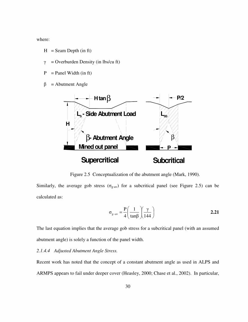
30
where:
H = Seam Depth (in ft)
γ = Overburden Density (in lbs/cu ft)
P = Panel Width (in ft)
β = Abutment Angle
H
Mined out panel
LS
Supercritical
- Abutment Angle
- Side Abutment Load
H tanβ
βP
SSL
P/2
Subcritical
β
Figure 2.5 Conceptualization of the abutment angle (Mark, 1990).
Similarly, the average gob stress (σg-av) for a subcritical panel (see Figure 2.5) can be
calculated as:
=−
144
γ
tanβ
1
4
Pσ avg 2.21
The last equation implies that the average gob stress for a subcritical panel (with an assumed
abutment angle) is solely a function of the panel width.
2.1.4.4 Adjusted Abutment Angle Stress.
Recent work has noted that the concept of a constant abutment angle as used in ALPS and
ARMPS appears to fail under deeper cover (Heasley, 2000; Chase et al., 2002). In particular,

31
for room-and-pillar retreat panels deeper than 1250 ft, it was found that a stability factor of
0.8 (for strong roof) could be successfully used in ARMPS, as opposed to a required stability
factor of 1.5 for panels less than 650 ft deep (MSHA, 2008). One of the more likely
explanations for this reduction in allowable stability factor is that the actual pillar abutment
loading may be less than predicted by using the constant abutment angle concept (Chase et
al., 2002). Colwell found a similar situation with deep longwall panels in Australia where
the measured abutment stresses were much less than predicted with a 21º abutment angle
(Colwell et al., 1999).
Since higher coal strengths have not been correlated with greater depth, it is most likely that
the lower stability factor is due to an overestimation of applied stress or load (MSHA, 2008).
Based on the NIOSH recommendations, it appears that the abutment loading based on the
constant abutment angle of 21° could be as much as 1.875 (1.5/0.8) times higher than actual
loading experienced in the field. Implementing this adjustment gives the following equation
for an adjusted average gob load for a subcritical panel based on the abutment angle concept
(given without derivation) (Heasley, 2008):
( )
∗∗
∗
−∗∗
−=−
144
γH
tanβ 4H
Ptanβ4H
1.5
0.81σ avadj-gob 2.22
where:
H = Seam Depth (ft)
γ = Overburden Density (lbs/cu ft)
P = Panel Width (ft)
β = Abutment Angle

32
The last equation modifies the abutment angle concept in an attempt to produce more
realistic results for panels deeper than 1250 ft.
Recent experience (Heasley, 2007) suggests that equation 2.21 provides a lower bound and
equation 2.22 provides an upper bound for realistic gob stresses estimation. Equation 2.19 is
between the interval given by the equations 2.21 and 2.22 and may provide a reasonable
starting point for further calibration. Regardless of which equation is chosen as a starting
point, it is clear that a realistic gob/abutment loading is critical in order to get a realistic
model result and that the gob stiffness should be carefully analyzed and calibrated in a
realistic model. A major improvement in mine design can be achieved by just getting the
designer to carefully consider the overburden load distribution between the gob and the
abutment (Heasley, 2008).
2.1.5 Calibrating Coal Strength.
Accurate in-situ coal strength is another value which is very difficult to obtain and yet is
critical to determining accurate pillar safety factors. It is difficult to get a representative
laboratory test value for the coal strength, and then scaling the laboratory values to accurate
in-situ coal pillar values is not very straightforward or precise (Mark and Barton, 1997).
2.1.5.1 Mark-Bieniawski Formula.
The default coal strength in LaModel, 900 psi, is used in conjunction with the Mark-
Bieniawski pillar strength formula (Mark, 1999):
−
+=
lh
w0.18
h
w0.540.64SS
2
ip 2.23
where:

33
Sp = Pillar Strength (psi)
Si = In-situ Coal Strength (psi)
w = Pillar Width
l = Pillar Length
h = Pillar Height
This formula also implies a stress gradient from the pillar rib that was previously presented in
equation 2.13 and is shown here:
+=
h
x 2.16 0.64S(x)σ ip 2.24
where:
σp(x) = Peak Coal Stress (psi)
x = Distance into Pillar
Si = In-situ Coal Strength (psi)
h = Pillar Height
The 900 psi in-situ coal strength that is the default in LaModel comes from the databases
used to create the ALPS and ARMPS program and is supported by considerable empirical
data. Mark and Barton, in 1997, showed that a uniform strength (900 psi) is a better
approximation than one based on laboratory testing. If the LaModel user chooses to deviate
very much from the default 900 psi, they should have a very strong justification, preferably a
suitable back analysis as described below or very accurate field measurements.

34
2.1.5.2 Back Analysis.
Heasley (2008) suggest that if for any reason, the user wants to get a representative coal
strength of the specific site conditions, the best technique to determine a more accurate coal
strength for LaModel is to back analyze a previous mining situation (similar to the situation
in question) where the coal was close to, or past, failure. Back-analysis is an iterative
process in which the coal strength is varied in order to find a value with model results that
fits with the actual observed failure. The previously determined optimum values of the
lamination thickness and gob stiffness should be, of course, used to perform the back analysis.
If there are no situations available where the coal was close to failure, then the back-analysis
can at least determine a minimum in-situ coal strength with some thought of how much
stronger the coal may be.
2.1.6 Calibration’s Implementation in LamPre3.0
2.1.6.1 Lamination Thickness Implementation.
In order to apply the calibration protocols, and equations described in the section 1.1.3.2 in to
the LaModel program, a simplified “Lamination Thickness Wizard” form (Figure 2.6) has
been added to the new LaMPre 3.0. This wizard implements the equations developed
previously (See section 1.1.3.2) in a user-friendly manner to assist the LaModel user in
calibrating the lamination thickness as suggested before (Heasley et al, 2010). The first
section of the form contains the “Rock Mass Parameters”. These values (Elastic Modulus,
Poisson’s Ratio and Vertical Stress Gradient) were previously entered in the “Rock Mass
Parameter” form in LaMPre and are used in the calculation, so they are displayed on this
form.

35
Figure 2.6 New Lamination Thickness Wizard form in LamPre3.0.
The next set of “Seam Parameters” (Elastic Modulus, Seam Thickness, Seam Depth, Width
of Gob and In-Situ Coal Strength) is the input that comes from the specific site and is critical
for calculating the rock mass lamination thickness (see Figure 2.6). Default values for the
Seam Elastic Modulus (300,000 psi) and In-Situ Coal Strength (900 psi) are provided, but
these values can be changed by the user if desired. In this section of the form, the user has to
enter the site specific values for the; Seam Thickness, Seam Depth and Width of Gob.

36
The third section of the form is for entering or calculating the extent of the abutment load
(see Figure 2.6). The first line in this section implements equation 2.2 and calculates the
extent of 90% of the abutment load based on field measurement and the given seam depth.
In the next line (“Extent of Abutment Load”), the user can enter a site specific value of the
abutment extent determined from field measurements, observations, etc., or the user can
check the box on the right (“Use the Suggested Value”) and the empirically suggested value
from the line above will automatically be entered for the extent of the abutment load to be
used in subsequent calculations. The third and last line in this section is the “Portion of Load
within the Given Extent” and this value has been fixed at 90% (0.90) for the calculation and
is displayed here for the user’s information.
The fourth section of the form is for entering or calculating the width of the yield zone. The
first line contains the “Suggested Percentage of the Overburden Load” determined by the
abutment angle concept as implemented in the equations for supercritical gob areas:
( )
×−=−
P
tanβHPσ %g 2.25
, or for calculating the average stress for subcritical gob stress:
( )
××−=−
tanβH4
P1σ avg 2.26
. In the next line (“Percentage of the Overburden Load”), the user can enter a site specific
value of the percentage of the overburden load determined from field measurements,
observations, etc., or the user can check the box on the right (“Use the Suggested Value”)
and the suggested value from the line above will automatically be entered for the percentage

37
of the overburden load to be used in subsequent calculations. Third line contains the “Trial
Lamination Thickness” which is used in equation 2.16 for calculating the yield zone. (The
trial lamination thickness default comes from the “Rock Mass Parameters” form and if it was
not changed there, it will be 50 ft, but is automatically updated when the lamination thickness
is calculated at the bottom of the form.) On the fourth line, there is a “Calculate” button and
the “Calculated Yield Zone” parameter. When the user clicks this yield zone Calculate
button, equation 2.16 is solved with the Trial Lamination Thickness and the other parameters
previously entered in the form and the resultant calculated width of the yield zone is shown
in the “Calculated Yield Zone” parameter box. In the fifth and last line of this section
(“Width of Yield Zone”), the user can enter a site specific value of the yield zone width
determined from field measurements, observations, etc., or the user can check the box to the
right (“Use the Calculated Value”) and the calculated value from the line above will
automatically be entered for the Width of Yield Zone to be used in subsequent calculations.
The final parameter line on the form contains a “Calculate” button and the “Calculated
Lamination Thickness” parameter. At this point, once the “Seam Parameters”, “Extent of
Abutment Load” and the “Width of the Yield Zone” have been input, the user can click the
lamination thickness calculate button and equation 2.12 will be used to calculate the
calibrated lamination thickness. If the “Use the Calculated Value” button is checked for the
“Width of the Yield Zone”, then a brief iteration will occur where the “Trial Lamination
Thickness”, “Width of Yield Zone” and “Calculated Lamination Thickness” are sequentially
updated until convergence on a final Width of Yield Zone and Calculated Lamination
Thickness. To use the Calculated Lamination Thickness for the input to LaModel, the user

38
clicks the “OK” button and the calculated lamination thickness is automatically entered as
the “Lamination Thickness” for the “Overburden / Rock Mass Parameters” from (See figure
2.7).
Figure 2.7 New Overburden / Rock Mass Parameters form in LamPre3.0.
So briefly, for the user to calculate a calibrated lamination thickness based on the
recommended calibration method presented here using the new Lamination Thickness
Wizard, they should:
a) Enter the site specific Seam Parameters
b) Enter a measured or observed Extent of Abutment Zone, or use the suggested value
c) Enter a measured or observed Width of Yield Zone, or use the calculated value
d) Calculate the calibrated Lamination Thickness.
2.1.6.2 Gob Stiffness Implementation.
To simplifying applying the derived equations in LaModel for determining the final gob
modulus, and to get the LaModel user to calculate and directly design the load distribution
between the gob and the abutments, a new wizard for defining the properties for the “Strain
39
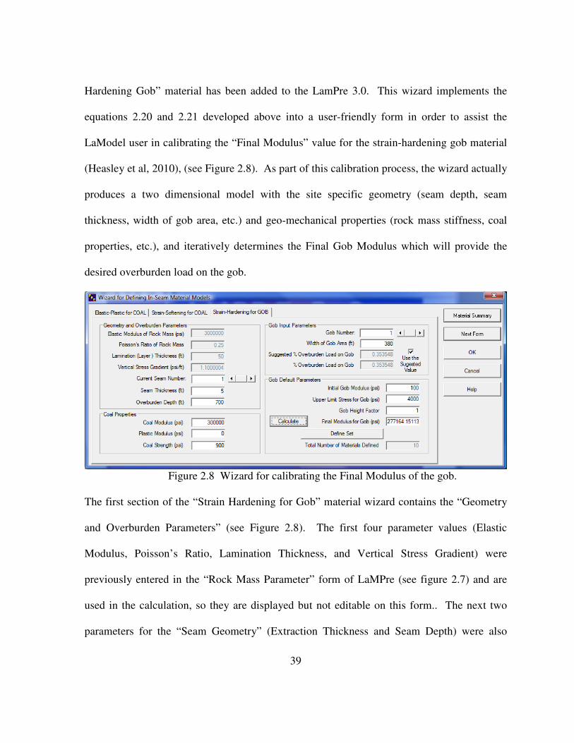
Hardening Gob” material has been added to the LamPre 3.0. This wizard implements the
equations 2.20 and 2.21 developed above into a user-friendly form in order to assist the
LaModel user in calibrating the “Final Modulus” value for the strain-hardening gob material
(Heasley et al, 2010), (see Figure 2.8). As part of this calibration process, the wizard actually
produces a two dimensional model with the site specific geometry (seam depth, seam
thickness, width of gob area, etc.) and geo-mechanical properties (rock mass stiffness, coal
properties, etc.), and iteratively determines the Final Gob Modulus which will provide the
desired overburden load on the gob.
Figure 2.8 Wizard for calibrating the Final Modulus of the gob.
The first section of the “Strain Hardening for Gob” material wizard contains the “Geometry
and Overburden Parameters” (see Figure 2.8). The first four parameter values (Elastic
Modulus, Poisson’s Ratio, Lamination Thickness, and Vertical Stress Gradient) were
previously entered in the “Rock Mass Parameter” form of LaMPre (see figure 2.7) and are
used in the calculation, so they are displayed but not editable on this form.. The next two
parameters for the “Seam Geometry” (Extraction Thickness and Seam Depth) were also

40
previously entered in the “Seam Geometry and Boundary Condition” form. These two
parameters can be set to the values previously entered for a particular seam by using the
“Seam Number” slider or can be manually changed as the modeler desires. These values
should be site specific.
The third set of parameters for the “Coal Properties” (Coal Modulus, Plastic Modulus and
Coal Strength) are used to define the nature of the coal yielding at the edge of the gob area
(see Figure 2.8). The initial values for these parameters are taken from those used in the
“Elastic-Plastic for Coal” material wizard, but the users can edit them in this form as they see
fit. It is highly recommended that the user keep the default properties for the coal strength,
but if either the coal strength or the coal modulus are changed, then they should be
consistently used between the “Elastic Plastic for Coal” wizard and the “Strain-Hardening for
Gob” wizard.
The fourth section of the form (Gob Input Parameters) is for entering or calculating the “%
Overburden Load on the Gob” (see Figure 2.8). The first line in this section is the “Gob
Number”. This refers to the number of the gob material which you are defining. The new
LamPre3.0 allows the user to define a variable number of gobs, each with different input
parameters. The input parameters for each of the defined gobs are then stored in the input
file. In this manner, the input file contains a record of the input parameters used to create
each gob and when the user reads a previously created input file into LamPre3.0, the
parameters used to create each gob are then available. The number of allowable gob
materials is determined by the number of defined material’s sets. The Current Gob Number
can be set to a particular gob number by using the “Gob Number” slider. The second line is
41
used for inputting the “Width of the Gob Area” for which the gob material properties are
desired. The user must input the site specific value here, but several different gob materials
(Gob Number) for different widths of gobs in different seams can certainly be developed.
The third line under “Gob Input Parameters” for the “Suggested % Overburden Load on the
Gob” implements equation 2.20 or 2.21 (as appropriate) to calculate the percentage of
overburden load on the gob based on the depth, gob width and abutment angle theory with a
default 21° abutment angle. In the fourth and final input line in this section (“% Overburden
Load on the Gob”), the user can enter a site specific value of the percent overburden load
determined from field measurements, observations, etc., or the user can check the box to the
right (“Use the Suggested Value”) and the suggested value from the line above will
automatically be entered for the “% of Overburden Load on the Gob to be used in subsequent
calculations.
The fifth section of the form is for calculating the “Final Gob Modulus” that will give the
user the desired gob loading. The first three parameters in this “Gob Default Parameters”
section contain default values for the: the Initial Gob Modulus, the Upper Limit Stress for the
Gob, and the Gob Height Factor. It is recommended the use of these default gob parameters,
but the form allows to a very experienced user to input other values. On the fourth line, there
is a “Calculate” button and the “Final Modulus” parameter. When the user clicks this final
modulus calculate button, the gob wizard takes the parameters input on the form and actually
produces a two dimensional model with a trial “Final Modulus”. For this trial final modulus,
the corresponding percentage of abutment load on the gob is calculated. The wizard then
continues to iteratively select better approximations of the Final Modulus until the Final Gob

42
Modulus which provides the desired percentage overburden load on the gob is determined.
This new gob material can then be entered as one of the model materials with the “Define
Set” button. The fifth line is for information purposes and shows the Total Number of
Materials Defined.
In review, the strategy to calculate a calibrated gob material based on the protocols and
equations presented here using the new “Strain-Hardening for Gob” material wizard, the
modeler should:
a) Enter the site specific Seam Geometry parameters
b) Enter the site specific Coal Properties
c) Enter the site specific gob width
d) Enter a measured or observed % Overburden Load on the Gob, or use the suggested
value
e) Calculate the calibrated Final Modulus for the gob.
2.1.6.3 Coal Strength Implementation.
To numerically simulate a yield zone in LAMODEL, concentric rings of different materials
are used against the openings and the material properties of the ribs are set such that the pillar
yields from the rib inward (Heasley et al, 2010). This type of yielding behavior matches that
observed in the field (see Figure 2.8). In the last few years, a systematic technique for
calculating these yielding coal properties based on the Mark-Bieniawski coal strength
formula (equation 2.23) and associated stress gradient (equation 2.24) has been developed
(Heasley et al, 2010). Essentially, for an element at the side of a pillar (such as A, C and E in

43
Figure 2.9), the element average peak strength is equal to the stress at the midpoint of the
element as determined by equation 2.27.
+=
h
x 2.16 0.64S(x)σ ip 2.27
For the corner elements, (such as B, D, F in Figure 2.9) which are needed to accurately
approximate the Mark-Bieniawski pillar strength, the “pyramid-like” geometry produces an
element average peak stress that is equal to the stress at the point one third of the distance
across the element as determined by equation 2.27.
Figure 2.9 Schematic of pillar loading and material code representation.
In order to assist the user in implementing the Mark-Bieniawski pillar strength formula in
LaModel, an improved wizard for defining the properties for the “Elastic-Plastic for Coal”
Load Bearing Capacity
LaModel Material Code
Representation
Rectangular Pillar
L
W
44
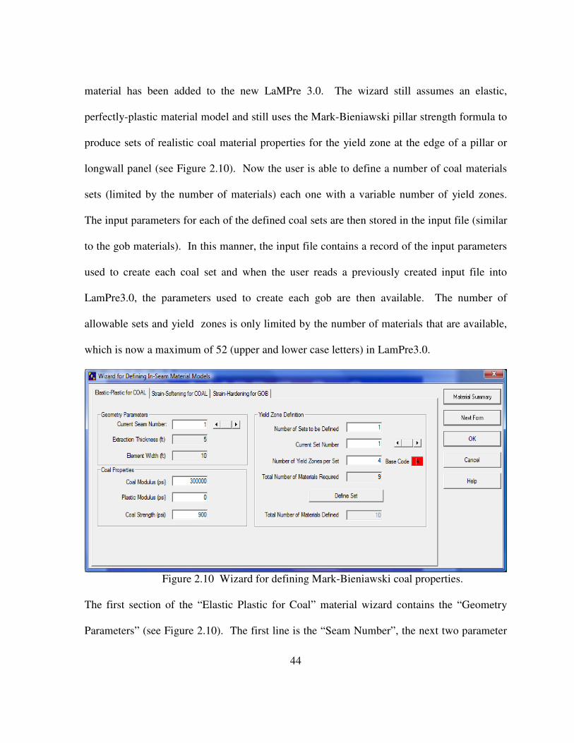
material has been added to the new LaMPre 3.0. The wizard still assumes an elastic,
perfectly-plastic material model and still uses the Mark-Bieniawski pillar strength formula to
produce sets of realistic coal material properties for the yield zone at the edge of a pillar or
longwall panel (see Figure 2.10). Now the user is able to define a number of coal materials
sets (limited by the number of materials) each one with a variable number of yield zones.
The input parameters for each of the defined coal sets are then stored in the input file (similar
to the gob materials). In this manner, the input file contains a record of the input parameters
used to create each coal set and when the user reads a previously created input file into
LamPre3.0, the parameters used to create each gob are then available. The number of
allowable sets and yield zones is only limited by the number of materials that are available,
which is now a maximum of 52 (upper and lower case letters) in LamPre3.0.
Figure 2.10 Wizard for defining Mark-Bieniawski coal properties.
The first section of the “Elastic Plastic for Coal” material wizard contains the “Geometry
Parameters” (see Figure 2.10). The first line is the “Seam Number”, the next two parameter

45
values (Extraction Thickness and Element Width) were previously entered in the “Seam
Geometry and Boundary Conditions” form of LaMPre and are used in the calculation, so
they are displayed on this form. The Extraction Thickness can be set to the value previously
entered for a particular seam by using the “Seam Number” slider. The Extraction Thickness
value is site specific and needs to be entered by the user.
The next set of “Material Parameters” includes: the Coal Modulus, the Plastic Modulus and
the Coal Strength. These coal properties are used to define the nature of the coal yielding at
the edge of the pillar. The program provides default values for these parameters. The Coal
Modulus can be modified to fit the user’s conditions. The Plastic Modulus is fixed at “0” psi
so that the wizard can accurate matches the Mark-Bieniawski pillar strength. The Coal
Strength defaults to 900 psi, and it can be changed, however, it is highly recommended that
the user keeps the default value for the coal strength, unless the user has a strong justification
for changing it. If either the coal modulus or the coal strength are changed, then they should
be consistently used between the “Elastic Plastic for Coal” wizard and the “Strain-Hardening
for Gob” wizard.
The third section of the form (Yield Zone Definition) is for defining the yield zones (see
Figure 2.10). The first line in this section is for choosing the number of sets of yield zones
that need to be defined. Typically, one set is defined for each seam with a different
extraction thickness. Also, the user has the option to define a different set of coal properties
for an older section of the mine or a section where the specific geology affects the pillar
strength. The next line contains the “Current Set Number”, which is the present set number
that is being defined and this number can be set in the edit box or by using the “Set Number”

46
slider. The third line is for specifying the “Number of Yield Zones per Set”. This is the
number of layers or concentric zones of different strength material that surround the pillar.
Each zone would be one element width, and the user should specify enough zones to cover
the expected yielding depth into the pillar. When the yielding coal properties are “Defined”,
an elastic core material is defined and then each zone will consist of two different materials,
a side material and a corner material. Therefore, a single cell deep yield zone requires 3
materials, a two cell deep yield zone requires 5, three deep requires 7, four deep requires 9
materials, etc. The “Base Code” displayed in the third line is the base or “core” material
code that is used to generate this specific yield zone set. This is the material code that will be
used in the grid generator to automatically add the yield zone. The next line is for
information purposes and shows the “Total Number of Materials Required”, that are the
number of materials required to perform the calculations set by the number of yield sets and
the number of yield materials per set. The next line contains the “Define Set” button for
actually calculating the yield zone properties and defining the materials in the program
database. When the Define Set button is clicked, the current Geometry Parameters and Coal
Properties are used to define the current set of yielding properties. This button needs to be
pressed and the calculation performed for each set of yielding properties (with different
Extraction Thicknesses, Coal Modulus or Coal Strengths). The last line in the “Yield Zone
Definition” section is for information purposes and shows the “Total Number of Materials
Defined” in the database using the “Define Set” button.

47
So briefly, for the user to define elastic-plastic coal properties which will match the Mark-
Bieniawski pillar strength formula in the “Elastic Plastic for Coal” material wizard, they
should:
a) Set the desired Extraction Thickness
b) Check or Enter the site specific Coal Properties
c) Set the number of Yield Coal Sets and the corresponding Zones per Set
d) Define each set into the material database.
2.2 Studies about LaModel.
From the very beginning in 1998, the LaModel program has been continuously upgraded (as
need arose) and modernized, as operating systems and programming languages have changed
(Hardy and Heasley, 1996; Heasley, 2008; Heasley and Tulu, 2011 and Whyatt et all., 2011).
This continuous upgrading implies continuous changes to the program that can result in the
obsolescence of the older versions.
The need to have accurate information about the LaModel program’s behavior due to the
changes on the input variables has been studied by several authors (Roberts et al., 2002;
Heasley and Tulu, 2011 and Whyatt et al., 2011).
Roberts et al. (2002), made a sensitivity analysis of LaModel software. They were trying to
determine the influence of mining parameters on pillar loads. They used LaModel software
varying the overburden stiffness and seam stiffness. They found that pillar loads decreased
with increasing overburden stiffness. They also observed that abutment loads increase as
pillar loads decrease. And that at large depths, high extraction and low overburden stiffness,
48
LaModel shows greatest deviations compared with tributary area theory. However, they
noted that, for typical mining parameters, the deviation from tributary area theory was less
than one percent.
After the collapse of the Crandall Canyon Mine in Utah on August 6th, 2007, several
questions were raised concerning the accuracy of the currently available analysis tools and
methods that can be used for the design of deep cover, pillar retreat mining sections (MSHA,
2008). One of the analysis tools that were used in the original design of the mine plan at
Crandall Canyon was the LaModel program. This program had a long history of successful
application at coal mines in the U.S. and around the world. So, why was the mine design
unsuccessful?
As a direct result of this tragic event, the existing pillar design analysis tools LaModel and
ARMPS, were re-evaluated for deep-cover pillar retreat (MSHA, 2008; Heasley, 2008;
Heasley, 2009a; Heasley, 2009b; Heasley, 2009c; Larson and Whyatt, 2009; Heasley et al.,
2010; Heasley and Tulu, 2011, Whyatt et all., 2011, etc.). As a result of this re-evaluation,
Heasley (2008) developed a standard method of calibrating LaModel; Heasley found that the
most critical input parameters with regard to controlling the mechanical response of the
program and for accurately calculating stresses and pillar safety factors are: The Rock Mass
Stiffness, The Gob Stiffness and The Coal Strength.
In 2008 (MSHA, 2008), Heasley conducted an extensive parametric analysis for LaModel, in
order to determine the optimum parameter values for matching the observed mine behavior,
to assess the sensitivity of the model results to the input values, and to investigate various
triggering mechanisms. As part of a parametric analysis of his back analysis (Heasley,
49
2009b), lamination thicknesses of 91, 152 and 183 m (300, 500 and 600 ft) were investigated.
He found that the 152 m (500 ft) value appeared to match the observed conditions best, also,
gob stress of around 6.2 MPa (900 psi) (60% abutment loading) was determined to be best
for matching the observations in the field. In the calibration process (Heasley, 2009a),
adjusted the coal strength until the calculated conditions matched the observed conditions as
closely as possible. The ultimate result of his coal strength calibration was an in-situ coal
strength value of 1325 psi as implemented in a strain-softening coal model. He found that in
general, the mine was primed for a massive pillar collapse because of the large area of fairly
equal size pillars with low safety factors. This large area of undersized pillars was the
fundamental cause of the collapse (MSHA, 2008; Heasley, 2009a and Heasley, 2009b).
In another instance, Heasley (2009c) conducted a case study of a pillar retreat mining section
in order to demonstrate the application of LaModel and the new calibration techniques. In
this case study, a comprehensive analysis of the stability of the barrier pillars, and of the
section pillars on retreat at a mine with similarities to the Crandal Canyon Mine was
performed. The back analysis used the recommended 900 psi coal strength and from the
LaModel analysis, there were no problems observed within the global stability of the section
and in general, the pillar retreat line was stable.
On the other hand, in 2009 Larson and Whyatt (Larson and Whyatt, 2009) used a generic site
model to compare the response of ALPS, LaModel, and FLAC in cases with a strong strata
member in the overburden. They said selecting the right program depends on understanding
the relative merits of these tools and their abilities to simulate ground response to mining in
the context of a particular site. They also said that LaModel uses only a fraction of the

50
parameters defined for the volume element model (FLAC) since fundamental assumptions in
the derivation of LaModel limit the range of material behavior. They incrementally reduced
the Young’s Modulus of the coal in order to simulate an incremental reduction of the applied
stresses to the excavation roof and floor. In their study, a wide range of results were
produced from small variations within a simple site model and choice of analysis method.
They also found that care must be taken when taking input parameters from past analyses
using different modeling programs. New models should be calibrated to field observations
and, ideally, measurements of critical behavior. As a conclusion, they said that the level of
effort required to achieve desired detail with a volume-element model may require much
larger preparation and computation times, possibly making approaches impractical or, in
some cases, practically impossible. The FLAC models described by them took up to 14 days
to solve with a modern workstation.
Heasley and Tulu (2011) published a sensitivity study for LaModel. A calibration procedure
was implemented by using the wizards in the new LaMPre 3.0 in order to produce a standard
model that fits within a verification database. They said it may guide a novice modeler in
choosing optimum input parameters and serve as a common basis for discussion of the model
design. They showed on their sensitivity analysis how the LaModel user could vary those
critical input parameters to adjust the model’s output, and using the recommended calibration.
They also found that changing the Poison’s ratio of the rock mass has a very minor effect on
the LaModel output.
Also in 2011, Whyatt et al. published a sensitivity analysis to LaModel program. They
performed an evaluation on how parameters, including datum location and overburden
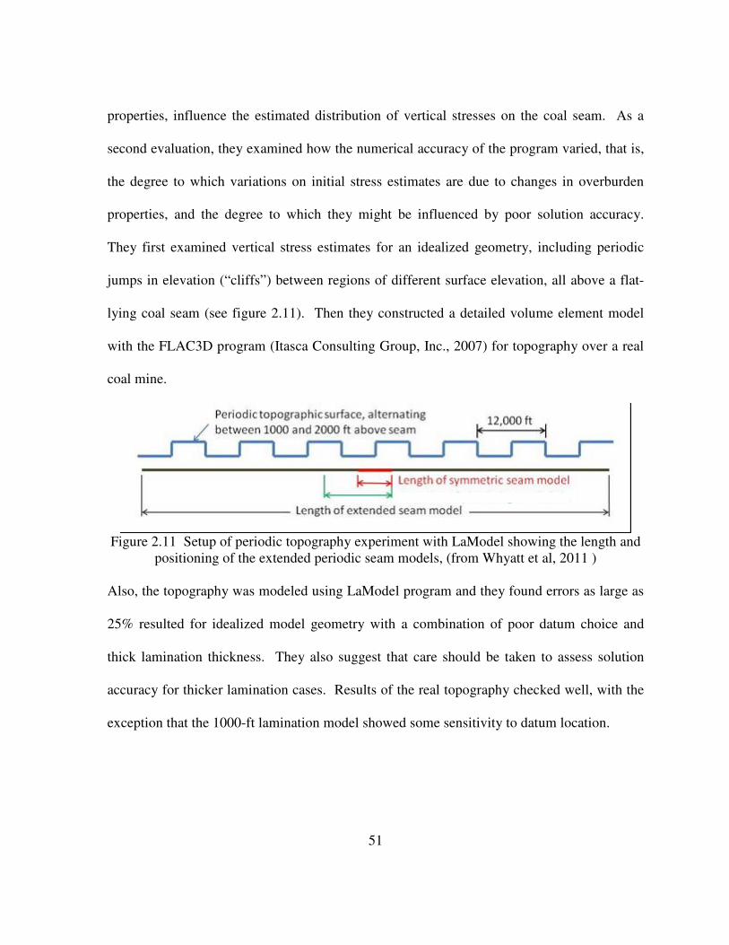
51
properties, influence the estimated distribution of vertical stresses on the coal seam. As a
second evaluation, they examined how the numerical accuracy of the program varied, that is,
the degree to which variations on initial stress estimates are due to changes in overburden
properties, and the degree to which they might be influenced by poor solution accuracy.
They first examined vertical stress estimates for an idealized geometry, including periodic
jumps in elevation (“cliffs”) between regions of different surface elevation, all above a flat-
lying coal seam (see figure 2.11). Then they constructed a detailed volume element model
with the FLAC3D program (Itasca Consulting Group, Inc., 2007) for topography over a real
coal mine.
Figure 2.11 Setup of periodic topography experiment with LaModel showing the length and
positioning of the extended periodic seam models, (from Whyatt et al, 2011 )
Also, the topography was modeled using LaModel program and they found errors as large as
25% resulted for idealized model geometry with a combination of poor datum choice and
thick lamination thickness. They also suggest that care should be taken to assess solution
accuracy for thicker lamination cases. Results of the real topography checked well, with the
exception that the 1000-ft lamination model showed some sensitivity to datum location.

52
2.3 Studies About LaModel Parameters.
Some researchers have been conducting studies on different fields including some of the
variables that LaModel uses. In 2003 a method was introduced by Ozbay and Rozgonyi for
estimating a range for strength parameters for coal pillars in order to be used in numerical
modeling. They used the finite difference code FLAC3D to develop a numerical model of a
two entry longwall system located at a depth of 2231 ft, with a panel length of 722 ft and a
mining height of 9.8 ft, modeling the coal seam as Mohr-Coulomb Strain-Softening (MCSS)
material and the gob as a non-linear elastic material. They found that the MCSS models
gives more realistic pillar load-deformation curves than the traditional Mohr-Coulomb (MC)
models. They also found that the MC model’s strength tends to increase rapidly, while the
MCSS model strength seem to follow the empirical strength trend.
Oraee et al., in 2008 published two strain-softening models for a series of yielding chain
pillars in a coal seam with a depth of 700 meters. They also did a sensitivity analysis to find
how sensitive the final design was to the pillar behavior after the coal peak strength. They
studied the behavior of yield pillars based on Hoek-Brown and FLAC strain-softening
models using three Hoek-Brown strain-softening models and seven FLAC strain-softening
models with different coal compressive strength. They also created four different models
varying the confinement stress in order to study the effect of confinement stresses on the coal
pillar strength. They also performed four different models with the FLAC strain-softening
model in order to evaluate the reliability of the safety factor application in yield pillar
designing. They said that the calculated safety factor based on conventional formulae is not

53
necessarily a perfect criterion. They found from the sensitivity analysis that the pillar
stability is highly sensitive to post peak behavior, whereas, the role of the uniaxial
compressive strength of the intact coal is not significant.
Jaiswal and Shrivastva in 2008 described an alternative approach for determination of strain-
softening constitutive behavior of coal-mass through back-analysis. The coal-mass was
assumed as the Hoek-Brown strain-softening material and dilation behavior was considered
as a function of confinement and plastic shear strain. They concluded from analysis that the
stress-strain behavior of the pillars generally lie in the elastic zone up to 2/3 of its peak
strength. They also proposed a statistical expression for estimating strength and post-failure
modulus of square pillar and a generalized strength formula and post-failure modulus for
Indian coal pillars.
In 1997, Mark and Barton created a comprehensive database that includes more than 4000
individual uniaxial compressive strength results for more than 60 coal seams. In their
statistical analysis they found no correlation between the stability factors of failed pillars and
coal specimen strength. They also found that there is no meaningful correlation between the
specimen strength and the in situ strength of US coal seams.
A research was conducted in 1993 by Papas and Mark where they collected a series of gob
moduli data for different types of rocks in order to perform a gob material simulation. They
said that the behavior of the gob is very important in understanding the complex ground
response to longwall mining. They said also that modelers in the past used estimates ranged
from 1000psi to over 300000psi and such variations greatly affected the outcome of the
54
numerical analyses, since the stiffness of the gob is a major component in the overall
behavior of the model. They also developed a load-deformation test procedure in order to
determine how the maximum particle size, shape, breakage, void ratio and rock strength
affect the stress-strain behavior of the simulated gob material. They found that at the lower
stress levels the stress versus strain curve is approximately linear which is consistent with
other author’s results. They used an analysis of variance applied to the test results to
determine if the rock type or particle size significantly affects the variables such as void ratio,
particle breakage, final shape ratio, secant modulus and/or tangent modulus. They found that
the void ratio, secant modulus, tangent modulus and most of the shape ratios are affected by
changing the rock type, but changes in the particle size do not significantly affect any of the
variables. They also developed equations using regression analysis to estimate the secant and
tangent modulus. Peng et al (1980) estimated that the gob modulus ranges from 13900 psi
for loosely packed gob to 139000 psi for partially failed gob. And lately, Hsiung and Peng
(Hsiung and Peng, 1985) used Peng’s rule of thumb (to determine the gob moduli for two
different rock types. They found that sandstone ranged from 50000 to 87000 psi and Shale
ranged from 20000 to 35000 psi.
In 1991, Salamon (Salamon, 1991) formulated a general frictionless laminated model whose
mathematical basis was the theory of thin plates. Also formulation assured that the
displacements and stresses are continuous across the layers. He showed in his work that,
when a distinct layer model can be approximated with its continuous version, the deviation
between solutions is small.

55
Gercek in 2007 (Gercek, 2007) conducted a research about the Poisson’s Ratio values for
rocks. He said that the importance of this mechanical property has not been appreciated as
much as it deserves, since the values of Poisson’s Ratio reported for rocks only varies in a
narrow range. According to Gercek, some important points to be considered regarding
Poisson’s Ratio of coals may be summarized as follows.
a) As the carbon content of coal exceeds 90%, its dynamic elastic constants, including
Poisson’s Ratio, become increasingly anisotropic (i.e. transversely isotropic).
b) A value of υ= 0,346 was reported to be the representative Poisson’s Ratio for a
wide range of coal grades.
c) According to a series of investigations in which the static tests were performed on
laboratory specimens loaded perpendicular to bedding, Poisson’s Ratios of some
Turkish coals were found to be between 0.15 and 0.49.
2.4 Other Software Studies.
One of the first implementations of the displacement discontinuity method into a personal
computer code for calculating stress and displacement from multiple seams was performed
by Sinha in 1979 (Sinha, 1979) and was called MULSIM program. The MULSIM program
has been upgraded along the time. In 1992, it was upgraded to MULSIM/NL by the addition
of non-linear seam material models, calculations for determining the mechanical strain
energy changes associated with the seam materials, and a capability for “stepping” though a
series of mining sequences (Zipf, 1992a and Zipf, 1992b).
56
Mark and Bieniawski (Mark and Bieniawski, 1986) developed the Analysis of Longwall
Pillar Stability (ALPS) method in 1986, to answer the need for effective longwall pillar
design. The fundament of the ALPS method is that there is a strong correlation between
pillar performance and gate entry stability. ALPS has the capability of estimating loads
applied to the gate pillars, determining the pillar strength and load-bearing capacity and
calculating a “stability factor” for the entire gate entry design (Iannacchione, 1988; Mark et
al., 1994 and Mark, 1992). The ALPS program was initially derived from underground
measurements of longwall abutment stresses and was later validated by the back-analysis of
more than 100 case histories (Mark and Chase, 1997).
The Analysis of Retreat Mining Pillar Stability (ARMPS) program was first introduced in
1995 (Mark et al., 1995). The ARMPS program estimates the loads applied to, and the load
bearing capacities of coal pillars used in retreat mining. It then calculates a stability factor
(SF) of the pillar section or “Active Mining Zone”. The formulas used in ARMPS are based
on those originally developed for the Analysis of Longwall Pillar Stability (ALPS) method
(Mark and Chase, 1997).

57
3 METHODOLOGY
3.1 General Description of the Methodology
This chapter presents the methodology used to determine the influence of input’s variation on
the output’s behavior for the LaModel program. A generalized and hypothetic set of input
parameters for the LaModel program is used here, and the steps adopted to conduct this study
included: a) the methodology is briefly described considering its limitations; b) data arrays
are designed and input files are created in order to drive the parametric analysis; c) the
changes in the LaModel’s output due to input variations are collected; d) the changes in the
output due to input variations are analyzed.
3.2 Parameter’s Description.
3.2.1 La Model’s Input Variables.
The LaModel program has many different types of input variables. Some variables come
from the mine design, such as the number of seams, pillar width or seam thickness; other
variables come from the seam geometry and location, such as the element width and the
overburden depth. Some other variables are used to define the rock mass state, such as the
rock mass modulus or the Poisson’s Ratio. Some variables are used for material definition,
such as the coal strength, coal modulus, or width of gob area. And in general, all of these
input variables help to define the mine situation in order to use the LaModel program. The
LaModel program provides default values for some of these input variables in order to help
with the model definition. These default values provided in LaModel can be used in many

58
practical situations, but in other situations, in which the mine conditions are well known or
similar mine conditions are applicable; site specific or calibrated values can be implemented
in to the LaModel program. Also, some times, laboratory test results or empirical data are
used as model input. Therefore, it is necessary to understand, how changing the values of the
input parameters could affect the model output.
The base model for this study was the LaModel tutorial #1, which is a classic and hypothetic
problem used to introduce the user to the LaModel program. The tutorial #1 input file is a
generic set of parameters and mostly consists of the default entry parameter values for
LaModel. The base model consist on a set of parameters with a single seam, 10 in seam
materials from A to J, and two steps, one for the development and other for the retreat mining.
The base model input parameters or Tutorial # 1 set is showed on the table 3.1
Table 3.1 Base model input parameters.
Parameter Value Units
Number of Seams 1 N/A
Number of In Seam Materials 10 N/A
Number of Steps 2 N/A
Poisson’s Ratio 0.25 N/A
Elastic Modulus 3000000 psi
Lamination Thickness 50 ft
Vertical Stress Gradient 1.1 psi/ft
Element Width 10 ft
Number of Elements in X Axis 100 N/A
Number of Elements in Y Axis 100 N/A
Overburden Depth 700 ft
Seam Thickness 5 ft
Seam Boundary Conditions Rigid N/A
Coal Modulus 300000 psi
Plastic Modulus 0 psi
Coal Strength 900 psi
Coal Poisson’s Ratio 0.33 N/A

59
Number of Sets 1 N/A
Yield Zones per Set 4 N/A
Width of Gob 360 ft
Peak Stress on the Gob 350 psi
Initial Gob Modulus 100 psi
Upper Limit Stress for the Gob 4000 psi
Gob Height Factor 1 N/A
Gob Load Ratio 0.7 N/A
Calculate Safety Factors True N/A
The rock mass parameters as well as the Poisson’s Ratio and the elastic modulus are the
default parameters for la model, the overburden depth is 700 ft, and the seam boundary
conditions are set as rigid (see table 3.1). A schematic representation of the Tutorial # 1
mining plan is showed on the figure 3.1, where the second step of the tutorial # 1 can be seen.
In the figure 3.1, the cross sections line A-A’, refers to the location of the middle of the gob.
This cross section will be used to study the output variations during the parametric analysis.
On the other hand, the figure 3.1 shows the pillars 1, 2 and 3 that will be used on the next
chapter to get the variation of the pillar stress safety factor.

60
Figure 3.1 Schematic representation of the tutorial #1 second step.
To perform the parametric analysis, variables were selected taking into account the
importance of each one at the time of the model’s evaluation. Most of the selected variables
are used to establish the mining situation but some of them also serve to establish the
problem’s accuracy. The selected variables can be encompassed into two groups: variables

61
related to the mining establishment and variables related to the model accuracy. The
following is a brief summary of the chosen variables and their importance for modeling.
3.2.1.1 Lamination Thickness.
In LaModel, the overburden loads are distributed by the laminated overburden model based
on the failure strength of the coal and the relative stiffness between the coal seam, gob and
overburden strata (rock mass). The Lamination Thickness quantifies the vertical thickness of
the geologic layers or laminations in the overburden. It represents an average vertical
distance between bedding plane slips or weakness in the overburden. The lamination
thickness does not necessarily have to correspond to the thickness of specific geologic layers;
rather it is a measure of the flexural rigidity of the overburden (Heasley K. A., 1998). In
general, thinner laminations create a less rigid overburden and increase the in seam
convergence, greater inter seam interactions, and steeper subsidence troughs. The lamination
thickness influences the effective stiffness of the overburden and also influence both pillar
stresses and convergence. Therefore the lamination thickness is a parameter that plays an
important role on the model calculations and its variations effects on the model results should
be studied.
3.2.1.2 Coal Strength.
One of the most important parameters in coal pillar design is the coal strength and it has been
actively studied from early 1900’s (Mark and Barton, 1997). Coal strength is the
determining factor in the design of effective pillars and barriers. It is also one of the most
difficult parameters to measure in mining and according to Heasley (2008), the best way to
determine it, is to back analyze a previous mining situation (similar to the situation in

62
question) where the coal was close to, or past, failure. Due to the importance of this factor
and because it is difficult to obtain from laboratory tests, the coal strength should almost
always be inferred or taken from a previous mining situation. With no certainty that the
selected coal strength value is close to the real value, a study of possible variations in the
LaModel output due to changes in the coal strength should be performed.
3.2.1.3 Rock Mass Modulus.
The rock mass elastic modulus of deformation is one of the most important input parameters
in numerical calculations for rock mass stability. It is well known, that the rock mass
modulus is another parameter that is hard to estimate. Palmström and Singh in 2001 said that
all in situ measurements of the static modulus of deformation used today are time-consuming
and incur notable costs and operational difficulties. Because of this, the deformation
modulus is often estimated indirectly from rock mass classification systems. In other cases
the modulus is assumed based on the experience of the engineering geologist or from
literature data. Therefore, variations on the rock mass modulus and their effects on the
LaModel outputs should be studied.
3.2.1.4 Coal Seam Modulus.
Another LaModel’s parameter that is not often considered in any detail is the elastic modulus
of the coal seam (Heasley and Tulu, 2011). For a calibrated model an increase or decrease in
the coal seam modulus will causes a decrease or increase respectively in the calibrated
lamination thickness in order to match the results keeping the desired abutment extent. As
the coal modulus is a parameter that is often empirically obtained or determined by
laboratory test, variations of the chosen coal modulus from the real coal modulus could be

63
important. Therefore, variations on the coal seam modulus and their effects on the LaModel
outputs should be studied
3.2.1.5 Poisson’s Ratio.
The Poisson's ratio of a material is the absolute value of the ratio of transverse strain to the
corresponding axial strain in a body subjected to uniaxial stress. Compressive deformation is
considered positive and tensile deformation is considered negative. When a compressive
force is applied to a body in one direction, other forces are induced in that body at right
angles to the applied force. The ratio of the induced forces to the applied force is given by
the Poisson's ratio. Typical values of Poisson's ratio for geologic material range from about
0.10 to 0.40 (Gercek H., 2007). The default value for LaModel is 0.25 and the Poisson's ratio
cannot be negative nor can it be greater than 0.50. The value of the “Poisson’s Ratio” does
not play an important role on the stress and displacement calculations in LaModel.
Although the use of approximate or typical values in most rock mechanic applications does
not create significant problems, Poisson’s Ratio plays an undeniably important role in the
elastic deformation of rocks and rock masses subjected to static or dynamic stresses (Gercek,
2007). It is utilized in rock engineering problems associated with the deformation of rocks,
e.g. it is a required computational input for the numerical stress analyses. A Poisson’s Ratio
value of 0.346 was reported to be the representative Poisson’s Ratio for a wide range of coal
grades (Szabo, 1981).
3.2.1.6 Grid Element Size.
The grid element size is a variable used to define the size of the minimum square element
used in the model. Depending on the element size, the accuracy of the model will be affected.

64
A big element size could cause inaccurate output values or numerical instability, because due
to the model resolution, some small features could not be taken in to account by the program
calculations. An small element size could add difficulties to create the model and as well as
increase the processing time. Also, there is no assurance that the output will be improved.
Therefore, it is necessary to optimize the element size in order to obtain reliable results in the
shortest possible time without compromising the model accuracy.
3.2.1.7 Surface Effects.
The Free Surface Effects check box causes the program to take into account the existence of
the ground surface. The LaModel is based upon a solution which assumes an infinite rock
mass. This assumption introduces errors which in practice are small unless the area to be
modeled is narrower than the overburden depth. In addition, since LaModel models must be
calibrated by adjusting the lamination thickness or rock mass modulus, the errors introduced
by ignoring the Free Surface Effects can generally be taken into account by adjusting either
or both of those two parameters. In shallow excavations, the proximity of the surface may
influence the stresses and displacements within the seam. LaModel models this effect by
placing a mirror-image seam in space such that a traction-free surface, representing ground
level. Taking into account the Free Surface Effects can drastically increase solution times,
since it requires the introduction of a “mirror image” seam, with a drastic increase in the
required number of computations due to the interactions between the elements of the real and
mirror image seams. The expected outcome of including the Free Surface Effects in the
analysis is to correct for near surface effects on the convergence, subsidence, and stresses.

65
Therefore, applying these corrections will result on different model’s output, and then is
necessary to study these differences.
3.2.1.8 Base Model, Calibrated and Uncalibrated Model.
Now that the necessary parameters have been briefly described, is necessary to explain the
way in which the inputs for LaModel are going to be manipulated in order to get the
parametric analysis results. As stated before, the base model will be Tutorial # 1 but two
separated set of input files will be created. Henceforth it will be called uncalibrated model to
those set of input parameters which are not given any setting other than the variation of the
parameter under study. In the same way, it will be called calibrated model to those set of
input parameters which have been calibrated using the technique described by Heasley
(2008).
3.3 Parametric Analysis Description.
The parametric analysis consists of three phases. The first phase is to develop the LaModel
input files for the different model runs. This part was done using the new LaMPre 3.0
preprocessor. The second phase is to run these cases using LaModel 3.0. And the final
phase consists of analyzing the results from LamPlt 3.0. The results of interest are the
program run times, in-seam convergence, total vertical stress, pillar stresses, abutment
stresses, surface subsidence, and pillar safety factors.
3.3.1 Lamination Thickness Data Set.
The lamination thickness is one of the most important factors in LaModel because it interacts
with other factors like the gob modulus and it influences the stiffness of the overburden. If

66
the lamination thickness is changed, the deformations, stresses and other output parameters
could be affected. To perform the parametric analysis to the lamination thickness, the effects
of changes on the lamination thickness over the LaModel results was studied. Three
uncalibrated models and a model with the calibration proposed by Heasley (Heasley, 2008)
were used. Four different values of lamination thicknesses from 100 to 500 (including the
calibrated lamination thickness with the corresponding calibrated final gob modulus) were
used to create these four models. Those values were arbitrary selected, but the range of their
variation is expected to be a wide general range, so it can cover most of the the LaModel
user’s mine conditions.
Using the four values of lamination thickness shown at the table 3.2, the same number of
models were created with no other variation than the Lamination thickness (for the calibrated
model, the final gob modulus was also calibrated).
Table 3.2 Input changes on the lamination thickness.
LT1 LT 2 LT 3 LT 4
Value [ft] 100 300 408.47 500
3.3.2 Coal Strength Data Set.
For this parametric analysis, a minimum coal strength of 600psi, the default LaModel coal
strength of 900psi and maximum coal strength of 1400psi were used in order to study the
coal strength effects over the model results The 600psi and 1400psi values were selected so
we can study hypothetic variations of up to a 55% from the default input for the coal

67
strength in LaModel. Three uncalibrated models were created using the coal strength values
shown on the table 3.4.
Table 3.3 Input changes on the coal strength.
CS1 CS 2 CS 3
Value [psi] 600 900 1,400
Also, three calibrated models were created following the calibration procedure (Heasley,
2008) to calibrate the lamination thickness and the final gob modulus, but using the coal
strength values given at the table 3.4. The corresponding calibrated lamination thickness and
calibrated gob modulus for each coal strength value are presented on table # 3.5.
Table 3.4 Coal strength and corresponding calibrated values. Coal Strength [psi] Lamination Thickness [ft] Final Gob Modulus [psi]
600 408.47 1,960,624.25
900 408.47 1,997,469.27
1,400 408.47 2,020,905.52
3.3.3 Rock Mass Modulus Data Set.
The two primary parameters that control the stiffness of the overburden are the elastic
modulus (E) and the lamination thickness (t). Similar to the lamination thickness, increasing
the rock mass modulus will result in decreasing the convergence over the gob, the peak
abutment stress, and increases the extent of the abutment zone. To perform the parametric
analysis of the rock mass modulus, the effects of changes on the rock mass modulus over
calibrated models were studied. Three uncalibrated models where designed using three
different values of rock mass modulus as shown on the table # 3.6.
Table 3.5 Input changes on the rock mass modulus.
E1 E 2 E 3
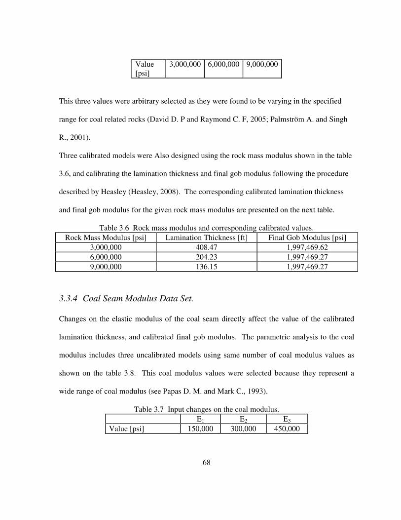
68
Value
[psi]
3,000,000 6,000,000 9,000,000
This three values were arbitrary selected as they were found to be varying in the specified
range for coal related rocks (David D. P and Raymond C. F, 2005; Palmström A. and Singh
R., 2001).
Three calibrated models were Also designed using the rock mass modulus shown in the table
3.6, and calibrating the lamination thickness and final gob modulus following the procedure
described by Heasley (Heasley, 2008). The corresponding calibrated lamination thickness
and final gob modulus for the given rock mass modulus are presented on the next table.
Table 3.6 Rock mass modulus and corresponding calibrated values.
Rock Mass Modulus [psi] Lamination Thickness [ft] Final Gob Modulus [psi]
3,000,000 408.47 1,997,469.62
6,000,000 204.23 1,997,469.27
9,000,000 136.15 1,997,469.27
3.3.4 Coal Seam Modulus Data Set.
Changes on the elastic modulus of the coal seam directly affect the value of the calibrated
lamination thickness, and calibrated final gob modulus. The parametric analysis to the coal
modulus includes three uncalibrated models using same number of coal modulus values as
shown on the table 3.8. This coal modulus values were selected because they represent a
wide range of coal modulus (see Papas D. M. and Mark C., 1993).
Table 3.7 Input changes on the coal modulus.
E1 E2 E3
Value [psi] 150,000 300,000 450,000

69
The parametric analysis to the coal modulus also includes three models using the calibrated
lamination thickness and calibrated final gob modulus and the coal modulus values given on
the table 3.9. The corresponding calibrated lamination thickness and final gob modulus for
the given coal modulus are presented on the next table.
Table 3.8 Coal modulus and corresponding calibrated values.
Coal Modulus [psi] Lamination Thickness [ft] Final Gob Modulus [psi]
150,000 204.23 884,899.23
300,000 408.47 1,997,468.88
450,000 612.71 3,192,848.43
3.3.5 Poisson’s Ratio Data Set.
In order to investigate the sensitivity of LaModel to Poisson’s Ratio variations, three values
of Poisson’s Ratio were selected. The corresponding Poisson’s Ratio variations are shown
on the table # 3.10. They correspond to a typical rage of values for Poisson’s ration (Johnson,
R.B. and DeGraff, J.V. 1988; Gercek H., 2007,)
Table 3.9 Poisson’s Ratio interval of variation.
υυυυ1 υυυυ2 υυυυ3
Value 0.15 0.25 0.35
In order to see the effects of changing the Poisson’s Ratio on the uncalibrated model results
(see section 3.3.1.8), three uncalibrated models were created, one for each Poisson’s Ratio.
The only parameter changed in each model was the Poisson’s Ratio.
On the other hand, to study the effects of changing the Poisson’s Ratio on the calibrated
model results (see section 3.3.1.8), three calibrated models were created using Heasley’s
proposed calibration (Heasley , 2008). The Poisson’s Ratio values from the table 3.10 were

70
used to create these calibrated models and the resulting calibrated lamination thickness and
calibrated final gob modulus for each Poisson’s Ratio value are shown on table 3.11.
Table 3.10 Poisson’s Ratio and corresponding calibrated values.
υ Lamination Thickness [ft] Final Gob Modulus [psi]
0.15 415.72 1,924,110
0.25 407.12 1,924,110
0.35 393.88 1,924,110
3.3.6 Grid element size Data Set.
Four grid element sizes were selected to perform the parametric analysis. These values were
selected because they are the most commonly used by the LaModel users and are shown on
the table # 3.11.
Table 3.11 Variation of the grid element size.
Case 1 Case 2 Case 3 Case 4
Element Size [ft] 2 5 10 20
The objective is to compare the time consumed by LaModel processing each model with
each grid element size. It will be meaningless to compare the calibrated and uncalibrated
models, so four uncalibrated models, one for each grid element size were created in order to
study the effect of the grid element size over the LaModel resultsResults for each model with
a grid element size different than 10ft were compared with the 10 ft element size model
results in order to appreciate the LaModel’s output behavior due to changes on the grid
element size. Selection of the 10ft model was arbitrary, and it is solely for output
comparison purposes.

71
3.3.7 Surface Effects Data Set.
To study the impact of the surface effect on the LaModel results, eight models using four
different seam depths were created. The surface effect feature was used in four of these
cases using a different seam depth for each one. Similarly, four models were created using
the same variations in the seam depth but without using the surface effect feature, see table
3.13. The main objective is to compare the LaModel outputs at four different depths using or
not the surface effects.
Table 3.12 Use of surface effects relative to the mining depth.
Case
#1
Case #2 Case #3 Case #4 Case #5 Case #6 Case #7 Case #8
Overburden
Cover (ft) 700 700 500 500 300 300 100 100
Surface
Effect No Yes No Yes No Yes No Yes
3.4 Summary.
In this chapter, the methodology to perform a parametric analysis was detailed; the data to be
used on the parametric analysis was described and the variation intervals were proposed. A
parametric analysis is developed in the next chapter, and the corresponding results are
discussed appropriately.

72
4 PARAMETRIC ANALYSIS RESULTS
4.1 Parametric Analysis
4.1.1 Introduction.
A parametric analysis was performed in order to studythe LaModel’s output behavior due to
changes on its input variables. A generalized set of input parameters was selected and it
mostly consist on the default entry parameters values for LaModel. Two separated set of
input files were created. An uncalibrated model is a set of input parameters which were not
given any setting other than the variation of the parameter under study. In the same way, the
calibrated model is a set of input parameters which have been calibrated using the technique
described by Heasley (Heasley, 2008).
To perform the parametric analysis, variables were selected taking in to account the
importance of each one at the time to evaluate the model. The selected variables can be
encompassed in two groups: variables related to the mining establishment and variables
related to the model accuracy.
4.1.2 Sensitivity to Lamination Thickness.
For the laminated overburden models, the formula for the convergence of the seam in the
open panel (Sl) is given by (Heasley, 1998):
( )( ) ( )22
2112
xLE
H
txS l −
⋅−=
γυ 4.1
where:

73
E = the elastic modulus of the overburden
υ = the Poisson’s Ratio of the overburden
L = half-width of the panel
x = distance from the panel centerline
t = the lamination thickness
H = the seam depth
As the lamination thickness increases, the overburden becomes stiffer, and with a constant
gob material, the convergence over the opening should decrease (see the lamination thickness
in the denominator of the equation 4.1), the gob load should decrease, the abutment load at
the edge of the opening should spread further and the peak vertical stresses should decrease
too.
Figure 4.1 The effect of change the lamination thickness on the abutment stress.

74
The figure 4.1 shows clearly the expected behavior, where an increase in the lamination
thickness results in the decreasing of the peak abutment stress and extending the abutment
stress. This behavior, matched with the reported by Roberts et al. in 2002 and also reported
by Heasley and Tulu in 2011.
In the table 4.1, the effect of increasing the lamination thickness on the abutment stresses is
explained using the average vertical stress, and the maximum stress for each lamination
thickness. An increase in the lamination thickness from 100 to 500 ft produces a change on
the average vertical stress of about 17% and about negative 41% on the peak abutment stress.
Also, a change of about 4% on the average vertical stress was observed when the lamination
thickness was changed from the calibrated value (408.47ft) to values like 300ft or 500ft,
which means variations of 22% and 26% in the lamination thickness respectively. The table
4.1 also shows that the variation on the average vertical stresses are not as high as the
variations on the peak abutment stresses.
On the other hand, as stated before, on the table 3.3, the final gob modulus increases when
the lamination thickness increases. This behavior is due to the variation on the convergence
over the gob, which naturally decreases when the lamination thickness is increased (Heasley
and Tulu 2011) and therefore to compensate for the decreasing convergence and still
maintain the same average load on the gob, the final gob modulus must also increase.
Table 4.1 Average and maximum abutment stress variations depending on the lamination
thickness.

75
Lamination
Thickness 100 [ft] 300 [ft]
408.47 [ft]
Calibrated 500 [ft]
Average
Vertical
Stress [psi]
627.55 569.58 543 515.32
Variation % 0.00% -9.24% -13.47% -17.88%
Peak
Abutment
Stress [psi]
2945.80 2135.10 1870.60 1735.00
Variation % 0.00% -27.52% -36.50% -41.10%
The figure 4.2 shows the effect of varying the lamination thickness over the convergence. In
this figure, can be seen the decreasing of the convergence when the lamination thickness and
the final gob modulus increases. The higher convergence was observed at the lowest
lamination thickness

76
Figure 4.2 The effect of changing the lamination thickness over the convergence.
In the table 4.2, the effect of the lamination thickness on the convergence can be seen.
Decreases on the average convergence of up to 68.21% were found when changing the
lamination thickness from a 100 to 500 ft. With the same variation on the lamination
thickness, there were also found decreases on the maximum convergence of up to 77%, .
This shows that the convergence decreases when the lamination thickness increases, which
matches with the expected behavior explained by the equation 4.1.
Table 4.2 Average and maximum convergence variations depending on the lamination
thickness (100 ft as base model). Lamination
Thickness 100 [ft] 300 [ft]
408.47 [ft]
Calibrated 500 [ft]
Average
Convergence
[ft]
0.0070 0.0030 0.002 0.0022
Variation % 0.00% -57.78% -64.87% -68.21%
Maximum
Convergence
[ft]
0.0206 0.0069 0.0054 0.0047
Variation % 0.00% -66.31% -73.74% -77.05%
Table 4.3 shows the effect of the lamination thickness on the pillar safety factors . Changes
on the lamination thickness from the calibrated value to a different value (as 500ft for this
case), produces variations on the safety factor up to 9.3%. A change from the calibrated
value to a value of 300ft produces a small variation in the SF (in the order of about 1%).
Maximum variations of about 18% were observed when the lamination thickness is so far
from the calibrated value. A trend to increase the safety factor when the lamination thickness
increased was also observed. On the other hand, a rapid increase of the safety factor for
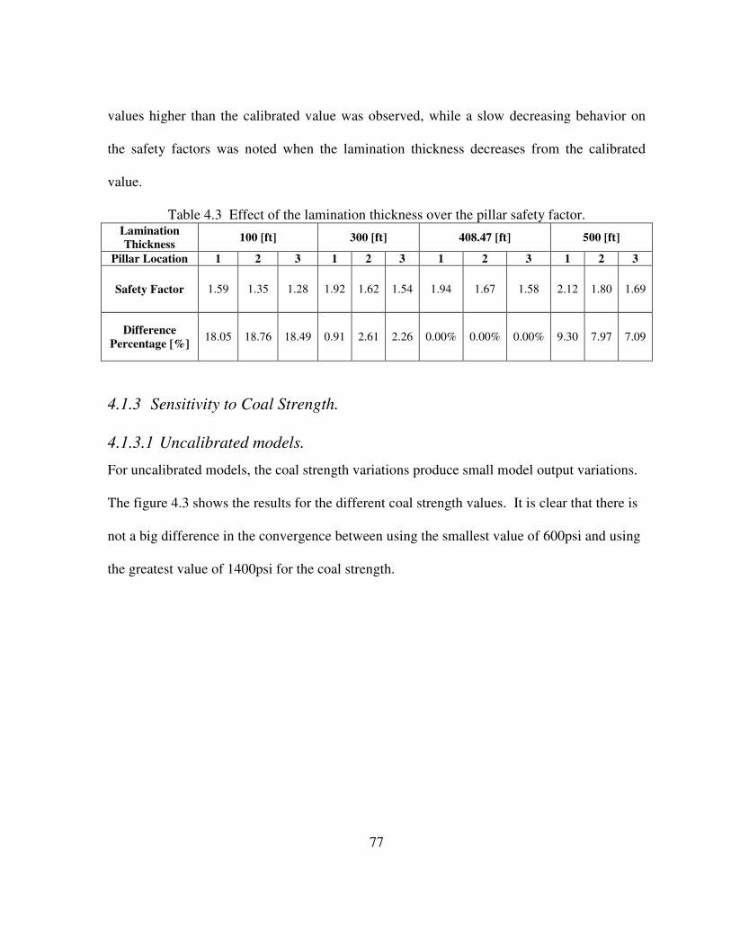
77
values higher than the calibrated value was observed, while a slow decreasing behavior on
the safety factors was noted when the lamination thickness decreases from the calibrated
value.
Table 4.3 Effect of the lamination thickness over the pillar safety factor. Lamination
Thickness 100 [ft] 300 [ft] 408.47 [ft] 500 [ft]
Pillar Location 1 2 3 1 2 3 1 2 3 1 2 3
Safety Factor 1.59 1.35 1.28 1.92 1.62 1.54 1.94 1.67 1.58 2.12 1.80 1.69
Difference
Percentage [%] 18.05 18.76 18.49 0.91 2.61 2.26 0.00% 0.00% 0.00% 9.30 7.97 7.09
4.1.3 Sensitivity to Coal Strength.
4.1.3.1 Uncalibrated models.
For uncalibrated models, the coal strength variations produce small model output variations.
The figure 4.3 shows the results for the different coal strength values. It is clear that there is
not a big difference in the convergence between using the smallest value of 600psi and using
the greatest value of 1400psi for the coal strength.

78
Figure 4.3 The effect of change the coal strength on the convergence.
On the other hand, Figure 4.4 shows the effect of changing the coal strength on the
convergence of the strata over the gob, for uncalibrated models. Differences are clearly
visible, and this figure also shows that increasing the Coal Strength does not necessarily
result in an increment of the vertical stress or vice versa..

79
Figure 4.4 The effect of change the coal strength on the abutment stress.
The figure 4.5 shows the effect of the coal strength on the pillar safety factor. It is clear that
increasing the coal strength and keeping constant the remaining values results on increasing
the pillar stress safety factors, as expected. That behavior is clearly noted on the figure 4.5,
for every pillar in consideration.
The trend is to increase when the coal strength is increased and to decrease from the pillar at
the edge of the panel to the center pillar. If the modeler is adjusting the coal strength, a
deviation from the real value could derive in stability problems during the mining activity.
Variations on the pillar stress safety factor were found to ranges between about 111% until
about 178% when the coal strength was varied from 600 to 1400 psi.

80
Figure 4.5 The effect of change the coal strength on the pillar stress safety factor.
It has to be noted that choosing the coal strength is a critical task, because a wrong coal
strength value may result in an artificially high or low safety factor, with the corresponding
devastating results for the mining activity.
4.1.3.2 Calibrated models.
For calibrated models, the coal strength variations produce a small convergence compared
with the uncalibrated models. The figure 4.6 shows the results for the different coal strength
values. Now, the change in the convergence due to variations in the coal strength is
graphically noticeable, but smaller than the results for uncalibrated models.

81
Figure 4.6 The effect of change the coal strength on the convergence for calibrated models.
Figure 4.7 shows the effect of changing the coal strength on the convergence of the strata
over the gob, for calibrated models. It is clear that for calibrated models, the vertical stress is
smaller than for the uncalibrated models. A smoothed behavior can be seen as the
differences between the results for different values of coal strength are smaller than the
differences for uncalibrated models...

82
Figure 4.7 The effect of change the coal strength on the abutment stress for calibrated
models.
The effect of the coal strength on the pillar stress safety factor is explained in detail on the
table 4.4. The trend for the safety factors is to increase when the coal strength gets increased.
If the modeler is adjusting the coal strength, a deviation from the real value could result in
stability problems during the mining activity. Table 4.4, also shows that when the coal
strength is varied from 600 to 1400 psi, the changes for the pillar stress safety factor are
biggest at the edge of the panel than in the center. This behavior matched with the expected
behavior, as pillars at the center of the panel will have higher stress levels than pillars at the
edge of the panel.
Table 4.4 Effect of the coal strength on the pillar stress safety factor.

83
Coal
Strength
[psi]
SF Pillar 1 SF Pillar 2 SF Pillar 3 Diff Pillar 1
[%]
Diff Pillar 2
[%]
Diff Pillar 3
[%]
600 1.4041 1.2914 1.2437 0.00% 0.00% 0.00%
900 1.9801 1.6965 1.6073 41.02% 31.37% 29.24%
1400 3.0978 2.6204 2.4492 120.63% 102.91% 96.93%
4.1.4 Sensitivity to Rock Mass Modulus.
4.1.4.1 Uncalibrated models.
The figure 4.8 shows the effect of changing the rock mass modulus with uncalibrated models
on the vertical stresses. The stresses over the gob appear to be increasing when the rock
mass modulus is decreased. There are similar values on the peak stresses and the abutment
extent decreases when the rock mass modulus decreases.
Figure 4.8 The effect of change the rock mass modulus on the convergence (uncalibrated
models).

84
Changes on the rock mass modulus without calibrating the lamination thickness should have
the same effect as the changes on the lamination thickness. It is something logic that if the
rock mass modulus increases keeping constant the remaining parameters, the convergence
will naturally decreases. In the figure 4.8 the behavior related before can be seen clearly.
On the other hand, the table 4.5 shows the average convergence, maximum convergence, and
percentage of variation for each rock mass modulus under study.
Table 4.5 Average and maximum convergence variations depending on the coal seam
modulus.
Rock Mass Modulus [psi] 3000000 6000000 9000000
Average Convergence [ft] 0.0100 0.0070 0.005
Variation % 0.00% 30.21% 47.35%
Maximum Convergence [ft] 0.030 0.021 0.015
Variation % 0.00% 32.18% 51.49%
In figure 4.9, a change of the rock mass modulus from 3000000 to 9000000 psi (200%)
produces changes on the average convergence of 47.35% and 51.49% on the maximum
convergence (see table 4.5).

85
Figure 4.9 The effect of change the rock mass modulus on the vertical stress (uncalibrated
models).
The table 4.6 shows the changes on the average vertical stress, peak stress and the
corresponding percentage of variation. There are not significant changes on the vertical
stresses when the rock mass modulus is changed. The maximum percentage of variation is
about 9% when the rock mass modulus is changed from 3000000 to 9000000 psi (200%).
Also, from the table 4.6, an increase on the peak stress when the rock mass modulus is
increased can be seen, so the peak stress increases when the rock mass modulus increases,
but the variation is too small (a variation on the rock mass modulus of the 100% produces a
variation on the peak stress of about 9%)

86
Table 4.6 Average vertical stress and peak abutment stress variations depending on the coal
seam modulus.
Rock Mass Modulus [psi] 3000000 6000000 9000000
Average Vertical Stress [psi] 669.71 627.71 607.57
Variation % 0.00% 6.27% 9.28%
Peak Stress [psi] 3229.7 2937.7 2578.2
Variation % 0.00% 9.04% 20.17%
4.1.4.2 Calibrated models.
If the rock mass modulus is changed while the lamination thickness and the final gob
modulus are calibrated, there are no changes on the model output. This behavior is due to the
lamination thickness calibration. When the lamination thickness is calibrated, the calibration
process produce a stress abutment extend that matches the value observed in the field and as
the rock mass modulus is included on the lamination thickness derivation, a change on the
rock mass modulus produces a change on the lamination thickness in order to match the
abutment extent. The related behavior was observed and the next two figures.

87
Figure 4.10 The effect of change the rock mass modulus on the vertical stress (calibrated
models).
Figures 4.10 and 4.11 shows that changing the rock mass modulus while calibrating the
lamination thickness and the final gob modulus, does not have any effect over the model
results.

88
Figure 4.11 The effect of change the rock mass modulus on the convergence (calibrated
models).
.
4.1.5 Sensitivity to Coal Seam Modulus.
4.1.5.1 Uncalibrated models.
The figure 4.12 shows the behavior of the convergence due to changes on the coal seam
modulus. On this figure it can be seen that changes on the coal modulus of up to 200 percent
does not produce high effects on the output for the convergence.

89
Figure 4.12 The effect of change the coal seam modulus on the convergence for uncalibrated
models.
The figure 4.13 shows the behavior of the vertical stress due to changes on the coal seam
modulus for uncalibrated models. On this figure it can be seen that an increase of the coal
seam modulus result in an increment of the peak abutment stress.

90
Figure 4.13 The effect of change the coal seam modulus on the abutment stress for
uncalibrated models.
4.1.5.2 Calibrated models.
In the equation 2.12, the elastic modulus of the seam is on the numerator, an increasing on
the coal seam modulus, will result on an increasing of the calibrated lamination thickness.
As the lamination thickness increases, the calibrated final gob modulus also increases in
order to keep the abutment load constant (see table 3.13).

91
Figure 4.14 The effect of change the coal seam modulus on the convergence for calibrated
models.
The figure 4.14 shows the effect of change the coal seam modulus on the convergence. As
changes on the coal seam modulus produces changes on the lamination thickness, and as
discussed before, as the lamination thickness increases, the convergence decreases.
Therefore, is to expect that the convergence should increase when the coal seam modulus
decrease. The figure 4.14 shows the related behavior, and it match with the results obtained
by Heasley and Tulu (2011).

92
Figure 4.15 The effect of change the coal seam modulus on the abutment stress for
calibrated models.
The figure 4.15 shows the effect of the changes on the coal modulus for the abutment stresses
on calibrated models. The results here, match with the Heasley and Tulu (2011) results.
When the coal seam modulus is changed, and the model is calibrated, the abutment stresses
are not affected in an important way.
The table 4.7 shows the average convergence, maximum convergence, and percentages of
variation for each coal seam modulus. Here can be seen that a variation from 150000 to
450000 psi (200%) on the coal seam modulus produces a change of about 66% on the
average of the convergence, and about 66% on the maximum convergence.
Table 4.7 Average and maximum convergence variations depending on the coal seam
modulus for calibrated models.

93
Coal Modulus [psi] 150000 300000 450000
Average Convergence [ft] 0.0050 0.0025 0.002
Variation % 0.0000% 49.8083% 66.481%
Maximum Convergence [ft] 0.011 0.006 0.004
Variation % 0.000% 49.762% 66.435%
On the other hand, the table 4.8 shows the average vertical stress, maximum vertical
abutment stress, and percentages of variation for each coal modulus. In this table, a non-
significant variation can be seen on the vertical stresses when the coal modulus is changed
and the model is calibrated. From the table 4.8, a variation from 150000 to 450000 psi
(200%) produces a change of about 0.6% on the average vertical stress, and a change of
about 0.5% on the peak stress.
Table 4.8 Average vertical stress and peak abutment stress variations depending on the coal
seam modulus for calibrated models.
Coal Modulus [psi] 150000 300000 450000
Average Vertical Stress [psi] 540.55 538.58 537.47
Variation % 0.00% 0.36% 0.57%
Peak Stress [psi] 1879.9 1886.7 1889.7
Variation % 0.00% 0.36% 0.52%
The table 4.9 shows the safety factors for each coal seam modulus in consideration. The
variations of the safety factor for each coal seam modulus and each pillar from the left edge
of the panel to the center (pillar 1, pillar 2, pillar 3) are shown in this table. The small
percentage variation indicates that there is not a significant variation on the safety factors
when changing the coal seam modulus.

94
Table 4.9 Pillar safety factor depending on coal seam modulus. Coal Modulus [psi] 150000 300000 450000
Pillar Location 1 2 3 1 2 3 1 2 3
Safety Factor 1.98 1.70 1.61 1.98 1.70 1.61 1.98 1.69 1.61
Difference Percentage
[%] 0.00% 0.00% 0.00% 0.19% 0.21% 0.20% 0.26% 0.29% 0.28%
Changes on the coal seam modulus of up to 200%, produces maximum changes of about
0.3% in the pillar safety factor.
4.1.6 Sensitivity to Poisson’s Ratio.
4.1.6.1 Uncalibrated models.
Figure 4.16 shows the effect of changing the Poisson’s Ratio on the convergence of the strata
over the gob for uncalibrated models. From this figure, it can be seen that an increase on the
Poisson’s Ratio produce a decreases on the convergence. A variation on the Poisson’s Ratio
from 1.5 to 3.5 (133.33%) changes the maximum convergence from 0.0305 ft to 0.0299 ft (-
1.795%).

95
Figure 4.16 The effect of changing the Poisson’s Ratio on the convergence over the
gob for uncalibrated models.
.
Figure 4.17 shows the behavior of the peak abutment stresses due to changes on the
Poisson’s Ratio. This figure shows the behavior of the peak abutment stresses due to
changes on the Poisson’s Ratio, this is showing that the peak abutment stress does not get
affected from these changes or the changes are very minor. This is explained in more detail
on the table 4.10.

96
Figure 4.17 The effect of changing the Poisson’s Ratio on the abutment stress for
uncalibrated models.
Table 4.10 shows average vertical stresses and peak stresses for uncalibrated models, along
with the corresponding percentage variations. From this table it can be extracted that
variations on the Poisson’s Ration don’t really affect the peak stress behavior, and it is clear
from this table, that a variation on the Poisson’s Ration of about 133% produces a really
small variation on the peak abutment stress (0.04%).
Table 4.10 Average vertical stress and peak abutment stress variations depending on the coal
seam modulus for uncalibrated models.
Poisson’s Ratio 1.5 2.5 3.5
Average Vertical Stress [psi] 671.35595 669.71621 667.16665
Variation % 0.00% 0.24% 0.62%
Peak Stress [psi] 3228.8 3229.7 3230.1

97
Variation % 0.00% 0.03% 0.04%
.
4.1.6.2 Calibrated models.
Figure 4.18 shows the effect of changing the Poisson’s Ratio on the convergence of the strata
over the gob. In this figure the change on the convergence is null, and it can be seen that for
calibrated models, there are no changes in the convergence due to changes in the Poisson’s
Ratio.
Figure 4.18 The effect of changing the Poisson’s Ratio on the convergence over the gob for
calibrated models.
On the other hand, changes in the vertical stresses due to variations in the Poisson’s ratio are
also not observed (see figure 4.19).
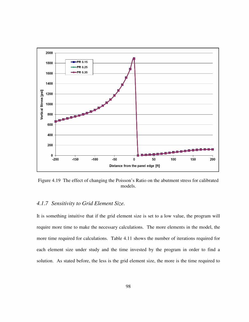
98
Figure 4.19 The effect of changing the Poisson’s Ratio on the abutment stress for calibrated
models.
4.1.7 Sensitivity to Grid Element Size.
It is something intuitive that if the grid element size is set to a low value, the program will
require more time to make the necessary calculations. The more elements in the model, the
more time required for calculations. Table 4.11 shows the number of iterations required for
each element size under study and the time invested by the program in order to find a
solution. As stated before, the less is the grid element size, the more is the time required to

99
find the solution. Also, the program requires les iterations if the grid element size is
increased.
Table 4.11 LaModel Running times and iteration number depending on the grid size.
Grid Element Size 2 [ft] 5 [ft] 10 [ft] 20 [ft]
Number of
iterations 10136 2188 605 225
Running Time
[seg] 93 5 1 ≈ 0
On the other hand, the table 4.12 shows the safety factor for each grid size on the three pillars
from the left of the panel at the retreat line to the center. Having the the 10 ft element size as
the comparison value, there is an increment on the safety factor for the first pillar when
usung 2ft, 5ft and 20ft of element size. The maximum difference of 2.08% was observed for
the 20 ft element size which means an increment from 1.59 to 1.623.
Table 4.12 Pillar safety factor depending on the grid size. Element Size 2 5 10 20
Pillar
Location 1 2 3 1 2 3 1 2 3 1 2 3
Safety
Factor 1.612 1.346 1.278 1.614 1.342 1.263 1.59 1.339 1.269 1.623 1.299 1.227
Difference
Percentage
[%]
1.38 0.52 0.71 1.51 0.22 0.47 0 0 0 2.08 2.99 3.31
Also from the table 4.12 it could be observed that there are not significant variations on the
pillar safety factor when the grid size is changed.
On the other hand, the effect of the grid element size on the convergence can be seen in
figure 4.19. Here it can be seen that when the grid element size is increased, but the
remaining parameters are kept constant, the amount of the convergence decreases, but not

100
0
0.05
0.1
0.15
0.2
0.25
0.3
0.35
0.4
0.45
-200 -150 -100 -50 0 50 100 150 200
5ft
0
0.05
0.1
0.15
0.2
0.25
0.3
0.35
0.4
0.45
-200 -150 -100 -50 0 50 100 150 200
10ft
0
0.05
0.1
0.15
0.2
0.25
0.3
0.35
0.4
0.45
-200 -150 -100 -50 0 50 100 150 200
20ft
significantly. This effect could be due to the decreasing of the resolution when the grid size
increases. The minor resolution means that the program will have less grid details to work
with, so the calculations could be affected by the lack of details.
0
0.05
0.1
0.15
0.2
0.25
0.3
0.35
0.4
0.45
-200 -150 -100 -50 0 50 100 150 200
Distance from panel edge [ft]
Co
nv
erg
ence
[ft
]
2ft
Figure 4.20 The effect of changing the grid element size on the convergence over the gob.
The table 4.13 shows the average and maximum convergence over the gob, for each grid size
under study. The average and maximum values for the 10 ft element size appears to be the
higher values, when compared with the 2, 5, and 20 ft element sizes.
Table 4.13 Average and maximum convergence variations depending on the grid size.
Grid Element Size 2 [ft] 5 [ft] 10 [ft] 20 [ft]
Average
Convergence [ft] 0.12845 0.12967 0.12998 0.12784
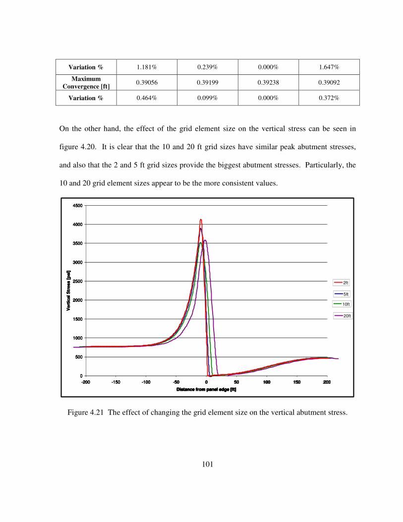
101
0
500
1000
1500
2000
2500
3000
3500
4000
4500
-200 -150 -100 -50 0 50 100 150 200
Distance from panel edge [ft]
Vert
ical S
tress
[p
si]
5ft
0
500
1000
1500
2000
2500
3000
3500
4000
4500
-200 -150 -100 -50 0 50 100 150 200
Distance from panel edge [ft]
Vert
ical S
tress
[p
si]
10ft
0
500
1000
1500
2000
2500
3000
3500
4000
4500
-200 -150 -100 -50 0 50 100 150 200
Distance from panel edge [ft]
Vert
ical S
tress
[p
si]
20ft
Variation % 1.181% 0.239% 0.000% 1.647%
Maximum
Convergence [ft] 0.39056 0.39199 0.39238 0.39092
Variation % 0.464% 0.099% 0.000% 0.372%
On the other hand, the effect of the grid element size on the vertical stress can be seen in
figure 4.20. It is clear that the 10 and 20 ft grid sizes have similar peak abutment stresses,
and also that the 2 and 5 ft grid sizes provide the biggest abutment stresses. Particularly, the
10 and 20 grid element sizes appear to be the more consistent values.
0
500
1000
1500
2000
2500
3000
3500
4000
4500
-200 -150 -100 -50 0 50 100 150 200
Distance from panel edge [ft]
Vert
ical S
tress
[p
si]
2ft
Figure 4.21 The effect of changing the grid element size on the vertical abutment stress.
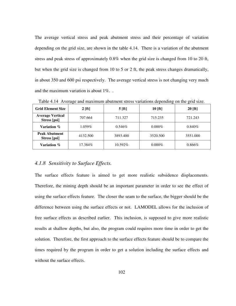
102
The average vertical stress and peak abutment stress and their percentage of variation
depending on the grid size, are shown in the table 4.14. There is a variation of the abutment
stress and peak stress of approximately 0.8% when the grid size is changed from 10 to 20 ft,
but when the grid size is changed from 10 to 5 or 2 ft, the peak stress changes dramatically,
in about 350 and 600 psi respectively. The average vertical stress is not changing very much
and the maximum variation is about 1%. .
Table 4.14 Average and maximum abutment stress variations depending on the grid size.
Grid Element Size 2 [ft] 5 [ft] 10 [ft] 20 [ft]
Average Vertical
Stress [psi] 707.664 711.327 715.235 721.243
Variation % 1.059% 0.546% 0.000% 0.840%
Peak Abutment
Stress [psi] 4132.500 3893.400 3520.500 3551.000
Variation % 17.384% 10.592% 0.000% 0.866%
4.1.8 Sensitivity to Surface Effects.
The surface effects feature is aimed to get more realistic subsidence displacements.
Therefore, the mining depth should be an important parameter in order to see the effect of
using the surface effects feature. The closer the seam to the surface, the bigger should be the
difference between using the surface effects or not. LAMODEL allows for the inclusion of
free surface effects as described earlier. This inclusion, is supposed to give more realistic
results at shallow depths, but also, the program could requires more time in order to get the
solution. Therefore, the first approach to the surface effects feature should be to compare the
times required by the program in order to get a solution including the surface effects and
without the surface effects.

103
Table 4.15 LaModel Running times and iteration number depending on the surface effects
feature. Overburden
Depth [ft] 100 300 500 700
Include
Surface
Effects
No Yes No Yes No Yes No Yes
Number of
iterations 153 243 442 608 796 1030 1148 1388
Running Time
[seg] ≈ 0 13 1 13 ≈ 0 13 1 13
The table 4.15 shows the iterations number and running time for each different overburden,
including and not including the surface effects. From the table 4.15, it is clear that including
the surface effects, makes the program running times increases, but that increasing on the
running times is not too high, so the running times when including the surface effects on the
model should not be a problem. Also, from the table 4.15, it can be seen that using the
surface effects increases the number of iterations.
Table 4.16 Effect of including the surface effects feature over the pillar safety factor. Seam
Depth [ft] 100 300 500 700
Pillar
Location 1 2 3 1 2 3 1 2 3 1 2 3
SF with
Surface
Effect 16
.82
15
.96
15
.91
4.8
0
4.2
3
4.0
9
2.7
0
2.3
0
2.1
7
1.9
3
1.6
6
1.5
7
SF without
Surface
Effect 16
.94
16
.11
16
.03
4.9
0
4.3
1
4.1
7
2.7
4
2.3
3
2.2
0
1.9
4
1.6
7
1.5
8
Difference
Percentage
[%] 0.6
9%
0.9
4%
0.7
2%
1.9
3%
1.9
5%
1.9
8%
1.4
3%
1.3
8%
1.3
4%
0.7
4%
0.7
1%
0.6
2%
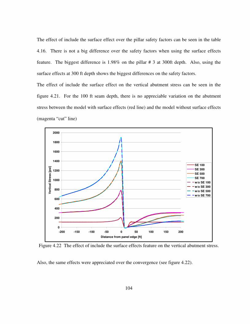
104
The effect of include the surface effect over the pillar safety factors can be seen in the table
4.16. There is not a big difference over the safety factors when using the surface effects
feature. The biggest difference is 1.98% on the pillar # 3 at 300ft depth. Also, using the
surface effects at 300 ft depth shows the biggest differences on the safety factors.
The effect of include the surface effect on the vertical abutment stress can be seen in the
figure 4.21. For the 100 ft seam depth, there is no appreciable variation on the abutment
stress between the model with surface effects (red line) and the model without surface effects
(magenta “cut” line)
0
200
400
600
800
1000
1200
1400
1600
1800
2000
-200 -150 -100 -50 0 50 100 150 200
Distance from panel edge [ft]
Ve
rtic
al
Str
es
s [
ps
i]
SE 100
SE 300
SE 500
SE 700
w/o SE 100
w/o SE 300
w/o SE 500
w/o SE 700
Figure 4.22 The effect of include the surface effects feature on the vertical abutment stress.
Also, the same effects were appreciated over the convergence (see figure 4.22).

105
0
0.001
0.002
0.003
0.004
0.005
0.006
-200 -150 -100 -50 0 50 100 150 200
Distance from panel edge [ft]
Co
nv
erg
en
ce
[ft
]
SE 100
SE 300
SE 500
SE 700
w/o SE 100
w/o SE 300
w/o SE 500
w/o SE 700
Figure 4.23 The effect of include the surface effects feature on the convergence.
The table 4.17 shows the effect of including the surface effects over the average vertical
stress, peak stress, average convergence and maximum convergence. There are not
differences over the average vertical stresses; the maximum difference is about 2%. Also,
there are not differences between the peak stresses when using or not the surface effect
feature.
Table 4.17 Effect of including the surface effects feature over the average vertical stress,
peak stress, average convergence and maximum convergence over the gob (a ‘Y’ indicates
using the surface effect, while ‘N’ indicates that surface effects feature was not used).
Seam Depth [ft] 100 300 500 700
Average vertical
stress [psi] Y 108.42 301.19 425.65 542.81
Average vertical
stress [psi] N 106.25 295.50 419.84 538.82
Difference
Percentage [%] 2.037% 1.925% 1.383% 0.741%
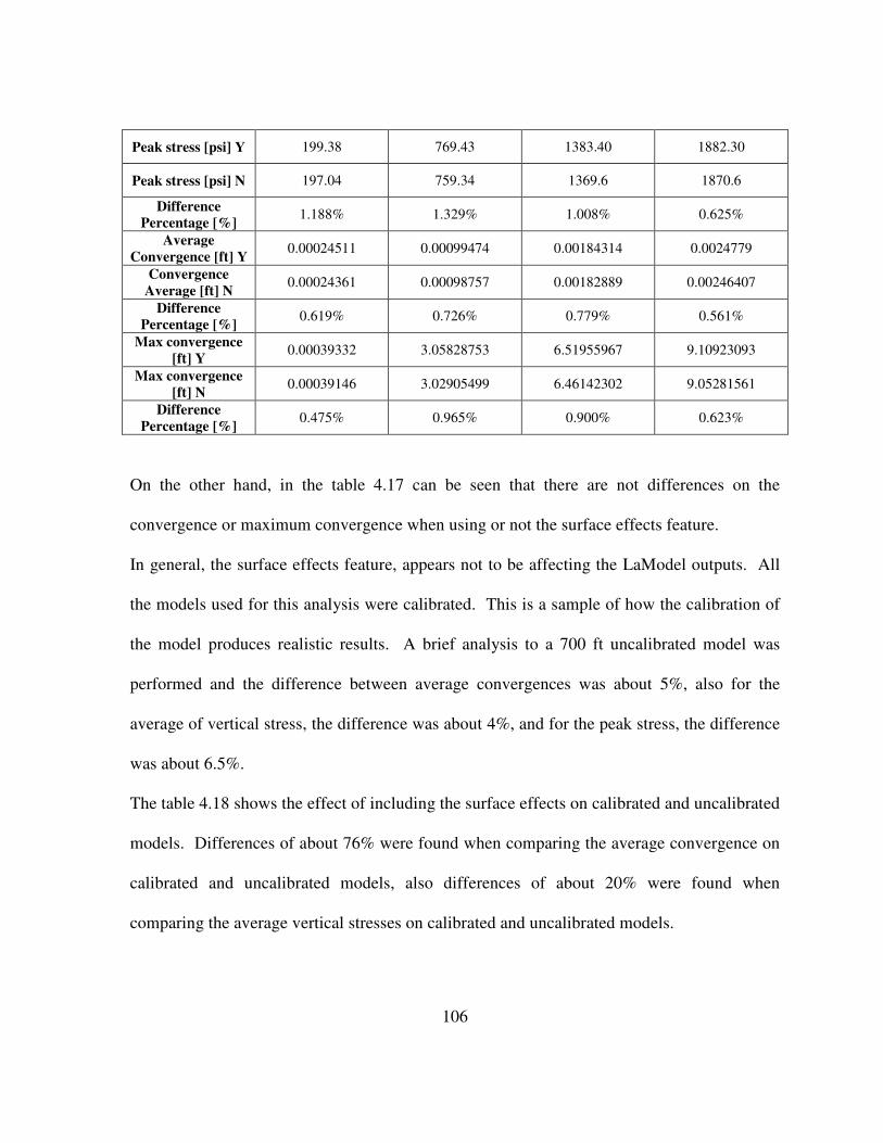
106
Peak stress [psi] Y 199.38 769.43 1383.40 1882.30
Peak stress [psi] N 197.04 759.34 1369.6 1870.6
Difference
Percentage [%] 1.188% 1.329% 1.008% 0.625%
Average
Convergence [ft] Y 0.00024511 0.00099474 0.00184314 0.0024779
Convergence
Average [ft] N 0.00024361 0.00098757 0.00182889 0.00246407
Difference
Percentage [%] 0.619% 0.726% 0.779% 0.561%
Max convergence
[ft] Y 0.00039332 3.05828753 6.51955967 9.10923093
Max convergence
[ft] N 0.00039146 3.02905499 6.46142302 9.05281561
Difference
Percentage [%] 0.475% 0.965% 0.900% 0.623%
On the other hand, in the table 4.17 can be seen that there are not differences on the
convergence or maximum convergence when using or not the surface effects feature.
In general, the surface effects feature, appears not to be affecting the LaModel outputs. All
the models used for this analysis were calibrated. This is a sample of how the calibration of
the model produces realistic results. A brief analysis to a 700 ft uncalibrated model was
performed and the difference between average convergences was about 5%, also for the
average of vertical stress, the difference was about 4%, and for the peak stress, the difference
was about 6.5%.
The table 4.18 shows the effect of including the surface effects on calibrated and uncalibrated
models. Differences of about 76% were found when comparing the average convergence on
calibrated and uncalibrated models, also differences of about 20% were found when
comparing the average vertical stresses on calibrated and uncalibrated models.

107
Table 4.18 Effect of including the surface effects feature over calibrated and uncalibrated
models (a ‘Y’ indicates using the surface effect, while ‘N’ indicates that surface effects
feature was not used).
Seam Depth [ft]
700
Difference [%]
Calibrated model Uncalibrated Model
Average vertical stress [psi] Y 542.813 668.44828 -18.80%
Average vertical stress [psi] N 538.82229 692.8007 -22.23%
Average Convergence [ft] Y 0.0024779 0.01064342 -76.72%
Convergence Average [ft] N 0.00246407 0.01014028 -75.70%

108
5 CONCLUSIONS AND FUTURE WORK
The main objective of this thesis was to develop a parametric analysis in order to establish, or
study all the LaModel’s possible output combinations of changes due to different changes on
the input variables. Variables as the Lamination Thickness, Coal Strength, Rock Mass
Modulus, Coal Modulus, Poisson’s Ratio, Grid Element Size, and Surface Effects were
studied here on this research effort.
As stated before, the main contribution of this study is the developing of a parametric
analysis for the LaModel program. After the parameters were varied in LaModel, the results
on the model output were studied by comparing the variations in seam displacement, vertical
stress, safety factors, and subsidence. This comparative analysis was performed by using
statistical techniques which included the use of the mean, maximum and minimum values.
Statistical measurements like the mean value, the maximum and the minimum values were
used for all the outputs in consideration. Here the main idea was to find tendencies in the
behavior of the output due to variations in the input variables. Averages, maximum or
minimum values are not always meaningful within the mining environment or as a
measurement of the LaModel outputs, but they are really meaningful as a statistic of the
outputs for LaModel and its corresponding behavior, and thus these values are helpful to
understand how the output is behaving due to changes in the input. Other measurements like
the percentage of the differences between some values were used in order to find how big is
the change in the output, and the possible relationship of the output values due to changes on
the input variables.

109
The lamination thickness is one of the most important factors in LaModel because it interacts
with other factors like the gob modulus and it influences the stiffness of the overburden. If
the lamination thickness is changed, the deformations, stresses and other output parameters
could be affected. Four models with the lamination thickness shown in table 5.1 were
studied.
Table 5.1 Input changes on the lamination thickness.
LT1 LT 2 LT 3 LT 4
Value [ft] 100 300 408.47 500
As a final result of this study, there was proved that the lamination thickness is one of the
driven variables of the underground mine design with LaModel, as it influences the
convergence and vertical stresses, and thus the safety factor calculation.
Influence of changes in the lamination thickness proposed on table 5.1 produced responses
on the average vertical stress with a maximum of about 17%, when lamination thickness was
ranged from 100ft to 500ft, and similarly, for the peak abutment stress a maximum variation
of about 41% was found when the lamination thickness was varied from 100ft to 500ft.
On the other hand, changes on the average convergence of up to 68.21% were observed when
changing the lamination thickness from a 100 to 500 ft. And changes of about 77% in the
maximum convergence were also noted with the same range of variation for the lamination
thickness. A negative trend of the convergence was found when increasing the lamination
thickness, and this negative behavior means that the convergence decreases when the
lamination thickness increases, which matches with the expected behavior explained in the
equation 5.1

110
( )( ) ( )22
2112
xLE
H
txS l −
⋅−=
γυ 5.1
Maximum variations on the safety factor of up to 18% were observed when the lamination
thickness was changed from the base value, which was the calibrated lamination thickness
(408.47ft), to a value of 100ft. A trend to increases the safety factor when the lamination
thickness increases was also observed.
Another value which is very difficult to obtain is the coal strength, and this is a critical value
in order to determine accurate pillar safety factors. LaModel uses a default value of 900psi
which is coming from the databases used in ALPS and ARMPS programs. If the LaModel
user chooses to deviate very much from the default 900 psi, they should have a very strong
justification, preferably a suitable back analysis.
For uncalibrated models, the coal strength does not show a really high instability for
convergence results or vertical stresses, but the safety factors are affected greatly. There
were found changes of up to 178% in the safety factors when using the different testing
values. For calibrated models, the coal strength variations produce a small convergence
compared with the uncalibrated models, and a smoothed behavior can be seen on the vertical
stresses when compared with the uncalibrated models.
Safety factor tends to increase when the coal strength is increased, and changes in the safety
factors for calibrated models were found to be of up to 120%.

111
There was also found that the behavior of the safety factors gets smoothed for the central
pillars when calibrating the model, while the behavior for the pillars on the edge seems to be
similar for calibrated or uncalibrated models.
If the modeler is adjusting the coal strength, a deviation from the real value could derive in
stability problems during the mining activity, as pillar safety factor are really sensitive to
changes on the coal strength, and this is an expected conclusion
As a result of this research, it has to be noted that choosing the coal strength is a critical task,
because a wrong coal strength value may result in an artificially high or low safety factor,
with the corresponding devastating results for the mining activity.
The coal seam modulus is one of the forgotten parameters, as it is not often considered, but it
is well known that it directly affect the resultant convergence. When coal seam modulus is
changed, but the abutment extent and load aren’t calibrated, the convergence and vertical
stresses will change. From the results, when the coal modulus increases, the convergence
will decrease and vice versa, which is the expected behavior. This behavior was observed on
the figure 4.12, and variations of the convergence when coal modulus was ranged from
150000 to 450000 were found to be of about 14%
On the other hand, a trend to increase the vertical stresses when the coal modulus increases,
was observed. Variations on the peak abutment stress were found to be of about 47% when
coal modulus ranged from 150000 to 450000.
For the calibrated model and variations of the coal modulus, a discussion regarding the
derivation of the equation 5.2 was given in the chapter two.

112
( )( )
22
s
0.1ln
dH5
h E
υ1 12E 2t
−−= 5.2
Results of the sensitivity analysis of the coal seam modulus for calibrated models are better
explained by using the above equation. On this equation, it can be seen that the coal seam
modulus is in the numerator of the equation, which means that the coal modulus is inversely
proportional to the calibrated lamination thickness. Therefore, any change in the coal seam
modulus, will affect the calculated lamination thickness, and this last will be adjusted in
order to keep the desired abutment extend. These changes in the lamination thickness will
affect the final gob modulus in the same way in order to keep the abutment load constant.
In other words, variations on the coal modulus in a calibrated model, will inversely affect the
convergence without affecting the seam stresses. This behavior was observed on the section
4.1.5.2, where variations of up to 66% (see table 4.8) in the seam convergence were found,
along with variations of up to 0.5% (see table 4.9) in the peak stress, which match with the
behavior above explained.
Poisson’s ratio is another of the forgotten parameters. From the equation 5.2, it can be seen
that the Poisson’s ratio acts always in the general form of:
( )2υ1 −
5.3
In this from, if Poisson’s ratio changes from 0.15 to 0.35 (about a 60% increase), the change
in the factor in the equation goes from about 0.98 to about 0.94 (about a 5% decrease), thus,
as a result of the equation 5.2, the effect of the Poisson’s ratio of the rock mass is almost

113
nothing. This behavior was observed for calibrated models, where effect of the variation of
the Poisson’s ratio over the convergence and vertical stresses was almost none (see section
4.1.6.1). The same behavior was observed for uncalibrated models (see section 4.1.6.1), and
as a conclusion of this research, it has to be noted that Poisson’s ratio plays a minimum roll
on the laminated model analysis.
The grid element size plays an important role on the model calculation due to its influence
over the results accuracy. It could be expected that the more elements in the model, the more
accurate the results could be, but at some point the gained accuracy due to adding elements to
the model could become meaningless. Data precision could play an important role on the
accuracy gained due to changes on the grid element size, but that was not object of this study.
Results showed an increment in the required time for calculations due to an increase in the
number of elements in the model, which was an expected result.
The behavior of the safety factors for the models under study varies depending on the pillar
in consideration, which says that there is not a real dependency on the safety factor behavior
due to the changes on the grid element size. In particular, for the pillar number 1, the
minimum safety factor (1.59, see table 4.13) was seen for the 10m grid element size, while
for second and third pillars (1.299 and 1.227 respectively), that minimum was observed for
the 20m element size. Maximum differences were observed when changing the grid element
size from 10m to 20m.
On the convergence side, there were not high changes in the convergence due to changes in
the grid element size. In general the variation was in third decimal digit, and as the 5m and
20m grid element size were the two minimum observed values for the maximum

114
convergences, it can be stated that changes in the grid element sizes are not high correlated to
changes in the maximum convergences. Furthermore, changes in the grid element size
produce no appreciable changes in the convergence output.
On the other side, minimum peak abutment stress of about 3520psi was observed for a 10m
of grid element size, while for the remaining grid element sizes; there were maximum
variations on the peak abutment stress of about 17%.
As a conclusion, appears like variations on the grid element sizes do not affect the behavior
of the convergence, but they could affect the behavior of safety factors and the maximum
abutment stresses. And on the other hand, changes on the grid element size directly affect
the time required for model calculations.
The surface effects feature is aimed to get more realistic subsidence displacements.
LAMODEL allows for the inclusion of free surface effects as described earlier Two different
studies were performed here, the first one was to compare the results by using and not using
the surface effects, while varying the seam depth, while the second one was keeping the seam
depth constant, and to compare calibrated and uncalibrated models.
For the calibrated models, the first approach to study the surface effects feature was to
compare the times required by the program in order to get a solution including the surface
effects and without the surface effects. In this regards, from the results on the table 4.16, it
can be stated that the time required to run a model by using the surface effects does not varies
regardless of the specific overburden depth. Time required running the model with surface

115
effects is higher than when running the model without the surface effects, but the difference
is not really high.
Pillar safety factors were also taken into account for this study, and the highest differences
between using and not using the surface effects were observed for 300m and 500m of seam
depths. Maximum differences of about 2% (see table 4.17) were observed.
On the other hand, no appreciable differences were observed on the average vertical stresses
and on the peak stresses when using or not the surface effect feature (see table 4.18). For the
convergence, the maximum observed changes were of about 1%, while for the peak stresses
this maximum was of about 1.3%. As a conclusion, in general, the surface effects feature,
appears not to be affecting the LaModel outputs when running a calibrated model.
On the uncalibrated model side, a brief analysis to a 700 ft uncalibrated model was
performed, and differences of about 76% were found when comparing the average
convergence on calibrated and uncalibrated models, also differences of about 20% were
found when comparing the average vertical stresses on calibrated and uncalibrated models
(see table 4.19). As a conclusion of this study, the surface effects do not play an important
role when running calibrated models, but it plays an important role when running an
uncalibrated model. This result may be due to the fact of using a calibrated lamination
thickness for the calibrated models, which takes in to account the seam depth and makes the
entire model to accommodate to the mining conditions due to the closeness of the surface.
As a parallel result of this research effort, the LaModel preprocessor “LaMPre 3.0” has been
updated so the user can conduct in an easily manner a systematic calibration process. For

116
this purpose, new forms as the Lamination Thickness Wizard have been added to this new
version, and other forms as the Coal Wizard and the Gob Wizard have been updated. The
latest version of the preprocessor, LaMPre 3.0, includes: a new strain–softening coal wizard
for developing calibrated post failure coal parameters, a renovated wizard to assist with the
development of “reasonable” gob properties based on a 2D laminated model, a new
lamination thickness wizard, a new overburden fault model, an energy release rate
calculation, and an expanded grid

117
6 REFERENCES
Broome J. B., (1997), “Development of a robust heat treating process for rockwell B-scale
hardness test blocks”, M.Sc. Dissertation, Massachusetts Institute of Technology, Jun, 108
pp
Chase F., Mark C. and Heasley K. A., (2002), “Deep Cover Pillar Extraction in the U.S.
Coalfields,” Proceedings of the 21st International Conference on Ground Control in Mining,
Morgantown, WV, Aug. 6-8, p. 68-80.
Colwell M., R. Frith and Mark C., (1999), “Analysis of Longwall Tailgate Serviceability
(ALTS): A Chain Pillar Design Methodology for Australian Conditions,” Proceedings of the
Second International Workshop on Coal Pillar Mechanics and Design, NIOSH: IC 9448, p.
33-48.
David D. P and Raymond C. F (2005) “Fundamentals of Structural Geology”, Cambridge
University Press, September 2005.
Gercek H., (2007), “Poisson’s Ratio values for rocks”, International Journal of Rock
Mechanics and Mining Sciences, Elsevier; Vol 44, 1–13.
Hardy R. and Heasley K. A., (2006), “Enhancements to the LaModel Stress Analysis
Program,” Proceedings of the SME Annual Meeting March 27-29 - St. Louis, Missouri
Heasley K. A., (2009a), “A Back Analysis of The Crandall Canyon Mine Collapse”, SME
Annual Meeting & Exhibit & CMA 111th National Western Mining Conference, Denver,
Colorado, Feb 22 – Feb 25.
Heasley, K. A., Sears M. M., Tulu I. B., Calderon-Arteaga C., and Jimison II L.W., (2010)
“Calibrating the LaModel Program for Deep Cover Pillar Retreat Coal Mining,” Proceedings
of the 3rd International Workshop on Coal Pillar Mechanics and Design, Morgantown WV,
July 26, 47-57.
Heasley K. A, (2000), “The Forgotten Denominator, Pillar Loading”, Proceedings of the 4th
North American Rock Mechanics Symposium, Seattle, WA, July 31-Aug. 3, p. 457-
464.
Heasley K. A., (2009b), “LaModel Analysis of The Crandall Canyon Mine Collapse”, 43rd
U.S. Rock Mechanics Symposium & 4th U.S. - Canada Rock Mechanics Symposium,
Asheville, North Carolina, June 28 – July 1.

118
Heasley K. A., (2009c), An Overview of Calibrating and Using the LaModel Program for
Coal Mine Design”, Proceedings of the International Workshop on Numerical Modeling for
Underground Mine Excavation Design, NIOSH, Pittsburgh, PA, June, pp 63 – 74.
Heasley K. A., (2008), "Some Thoughts on Calibrating LaModel", Proceedings of the 27st
International Conference on Ground Control in Mining, Morgantown, WV, Jul. 29-30.
Heasley K. A., (1998), "Numerical Modeling of Coal Mines with a Laminated Displacement-
Discontinuity Code", Ph.D. Dissertation, Colorado School of Mines, May, 187 pp
Hsiung S. M. and Peng S. S., (1985), “Chain pillar design for U. S. Longwall panels”, Min.
Sci. & technology, Vol 2, pp. 279-305.
Iannacchione A. T., (1988), “Behavior of a coal pillar prone to burst in the southern
Appalachian Basin of the U.S.”, 2nd Int. Symp. of Rockburst and Seismicity in Mines, Minn.,
NM, pp.427-439.
Itasca Consulting Group, Inc., (2007), “FLAC3D: Theory and Background”, Minnesota,
USA.
Jaiswal A., and Shrivastva B.K., (2008), “Numerical simulation of coal pillar strength”,
International Journal of Rock Mechanics and Mining Sciences, Vol 46, 779–788.
Mark C. and. Barton T. M, (1997), “Pillar Design and Coal Strength,” Proceedings of New
Technology for Ground Control in Retreat Mining, NIOSH IC 9446, p. 49-59.
Johnson, R.B. and DeGraff, J.V. (1988) Principles of Engineering Geology, Wiley
Karabin, G. and M. Evanto, (1999), “Experience with the Boundary-Element Method of
Numerical Modeling to Resolve Complex Ground Control Problems,” Proc. of the 2nd Intl.
Workshop on Coal Pillar Mechanics and Design, NIOSH IC 9448, p. 89-113.
Larson M.K. and Whyatt J.K., (2009), “Critical review of numerical stress analysis tools for
deep coal longwall panels under strong strata”, SME Annual Meeting and Exhibit. Preprint
09–011. Littleton, CO: Society for Mining, Metallurgy, and Exploration, Inc., 12 pages.
Mark C. and Bieniawski Z.T., (1986), “An Empirical Method for the Design of Chain Pillars
for Longwall Mining”. Proc. 27th U.S. Symp. on Rock Mech., Tuscaloosa, AL, pp. 415-422.
Mark C., Chase F., and Campoli, A. (1995); “Analysis of Retreat Mining Pillar Stability”:
Proceedings of the 14th Int. Conference on Ground Control, Morgantown, W.V., August,
1995.

119
Mark C. and Chase F., (1997), “Analysis of Retreat Mining Pillar Stability (ARMPS),”
Proceedings: New Technology for Ground Control in Retreat Mining, eds. C. Mark and R.
Tuchman, NIOSH IC 9446, March, pp. 17-34.
Mark C., (1990), “Pillar Design Methods for Longwall Mining”, BuMines IC 9247, 1990, 53
pp
Mark C., (1999), “Empirical Methods for Coal Pillar Design”, Proceedings of the Second
International Workshop on Coal Pillar Mechanics and Design, NIOSH IC 9448, p.
145-154.
Mark C., (1992), “Analysis of Longwall Pillar Stability (ALPS); an update”, Proceedings of
the Workshop on Coal Pillar Mechanics and Design, BuMines IC 9315, p. 238-249.
Mark, C., Chase, F. and Molinda, G., 1994, “Design of Longwall Gate Entry Systems Using
Roof Classification,” Proceedings of USBM Technology Transfer Seminar, Washington, D.
C., pp. 5-17.
METU., (1989a), “Investigation on the determination of rock mechanics and design
parameters for coal and coal measure rocks at Asma Mine”, Report prepared for TTK,
Department of Mining Engineering, Ankara.
METU., (1989b), “Investigation on the determination of rock mechanics and design
parameters for coal and coal measure rocks at Gelik Mine”, Report prepared for TTK,
Department of Mining Engineering, Ankara;.
METU., (1989c), “Investigation on the determination of rock mechanics and design
parameters for coal and coal measure rocks at Kandilli Mine”, Report prepared for TTK,
Department of Mining Engineering, Ankara.
MSHA, (2008) “Fatal Underground Coal Burst Accidents August 6 and 16, 2007, Crandall
Canyon Mine”, DOL-MSHA, RI, 472 pp.
Oraee, K., Hosseini, N., and Gholinejad, M., (2008), “Logical design of yield pillar base in
longwall Mining”, Proceedings of Seventeenth International Symposium on Mine Planning
and Equipment Selection (MPES 2008), Beijing, China, pp. 706-712.
Ozbay U. and Rozgonyi T. G., (2003), “Numerical Modeling of Stress and Deformations
Encountered in Deep Longwall Coal Mines Using Strain Softening Failure Criterion”,
International Conference on Safety and Environmental Aspects of Mining, A Publication of
the University of Miskolc Series A. Mining, Volume 63.
Palmström A. and Singh R., (2001), “The Deformation Modulus of Rock Masses -
Comparisons between in situ tests and indirect estimates”, Tunneling and Underground
Space Technology, Vol. 16, No. 3, pp. 115 - 131.

120
Papas D. M. and Mark C., (1993), “Behavior of Simulated Longwall Gob Material”, Report
of investigations, Bureau of Mines, RI9458, pp 39.
Peng S. S., Matsuki K. and Su, W. H., (1980), “3D Structural analysis of longwall panels”,
Paper in the state of the art in Rock Mechanics; Proceedings of the 21st U. S. Symposium on
rock Mechanics, compiled by D. A. summers (Rolla, MO, May 28-30) Univ, MO, pp. 44-56.
Peng S. S., (2006), Longwall Mining, 2nd edition, Department of Mining Engineering, West
Virginia University, 621 p.
Roberts D. P., van der Merwe J. N., Canbulat I., Sellers E. J. and Coetzer S., (2002),
“Development of a Method to Estimate Coal Pillar Loading”, Safety in Mines Research
Advisory Committee, COL 709, September, pp 1-90.
Salamon, M. D. G., (1967), “A study of the Strength of Coal Pillars”, Journal of the South
African Institute of Mining and Metallurgy, v 68, pp. 55-67.
Salamon, M. D. G, (1991), “Deformation of stratified rock masses: A laminated model”,
Journal of the South African Institute of Mining and Metallurgy, v 91, # 1, Jan, pp. 9-25.
Sinha K. P., (1979), “Displacement discontinuity technique for analyzing stress and
displacements due to mining in seam deposits. Dissertation. University of Minnesota.
Whyatt J. K., Larson M. K. and Heasley K. A., (2011), “Topography and Coal Seam Initial
Stress Estimation: a Sensitivity Study”, 30th International Conference on Ground Control in
Mining, Morgantown, WV, Jul. 26-28.
Zipf, R. K., (1992a), “MULSIM/NL Theoretical and Programmer’s Manual,” BuMines IC
9321.
Zipf, R. K., (1992b) “MULSIM/NL Application and Practitioner's Manual”, USBM
Information Circular 9322, 44 pp. 47.