Implementing a Stochastic Model for Oil Futures Prices

Gonzalo Cortazara, Eduardo S. Schwartzb

a

Departamento de Ingeniería Industrial y de Sistemas, Escuela de Ingeniería, Pontificia Universidad Católica de Chile, Vicuña Mackenna 4860, Santiago, Chile

bAnderson School at UCLA, 110 Westwood Plaza, Los Angeles, CA 90095-1481, USA

.

June 2002 Abstract

This paper develops a parsimonious three-factor model of the term structure of oil futures prices that can be easily estimated from available futures price data. In addition, it proposes a new simple spreadsheet implementation procedure. The procedure is flexible, may be used with market prices of any oil contingent claim with closed form pricing solution, and easily deals with missing data problems. The approach is implemented using daily prices of all futures contracts traded at the New York Mercantile Exchange between 1991 and 2001. In-sample and out-of-sample tests indicate that the model fits the data extremely well. Though the paper concentrates on oil, the approach can be used for any other commodity with well- developed futures markets.

JEL Classifications: G13 Q49 C52 Keywords:Crude Oil: Futures; Stochastic behavior; Model Implementation

1. Introduction This paper develops a parsimonious three-factor model of the term structure of oil futures prices that can be easily estimated from available futures price data. In addition, it proposes a new simple spreadsheet implementation procedure. The procedure is flexible, may be used with market prices of any oil contingent claim with closed form pricing solution, and easily deals with missing data problems. The approach is implemented using daily prices of all futures contracts traded at the New York Mercantile Exchange between 1991 and 2001. In-sample and out-of-sample tests indicate that the model fits the data extremely well. Though the paper concentrates on oil, the approach can be used for any other commodity with well-developed futures markets. In the last ten years there has been an increasing interest both by academics and practitioners in understanding the stochastic behavior of oil prices. This interest comes from increasing price volatility, which makes predictions more difficult. Also, modern asset pricing models of oil-related real assets such as oil-field development or extraction projects, consider these assets as real options contingent on the oil price level and its stochastic process (Paddock et al., 1988). In addition, pricing of new oil-linked financial instruments requires knowledge of the stochastic behavior of the underlying asset. Finally, commodity price risk, which can have a huge impact on a firm’s profits (Culp and Miller (1994)), may be successfully hedged to the extent that the stochastic process for the underlying commodity is known. It is well known that the futures price of a financial asset that pays no dividends is equal to the spot price of the asset plus the interest rate (carrying costs) over the life of the futures contract. Any dividend payment on the financial asset should be subtracted from the carrying costs. In the case of commodities, futures prices are normally lower than the spot price plus the interest rate over the life of the futures contract. This “shortfall”, which is like an implicit dividend that accrues to the holder of the spot commodity but not to the holder of the futures contract, is what is known as the convenience yield of the commodity (Brennan, 1991). Stochastic models of the behavior of commodity prices differ on the role played by the convenience yield and on the number of factors used to describe uncertainty. Early models assumed a constant convenience yield and a one-factor Brownian

2

motion (Brennan and Schwartz, 1985). This random walk specification for commodity prices was used until a decade ago, when mean reversion began to be included as a response to the evidence that volatility of futures returns declines with maturity. One-factor mean reverting models can be found for example in Ross (1995), Schwartz (1997), Cortazar and Schwartz (1997), Laughton and Jacoby (1993 and 1995). An undesirable implication of one-factor models, however, is that all futures returns are perfectly correlated, a fact that defies empirical evidence. To account for a more realistic stochastic behavior, two-factor models with mean reversion were introduced. Examples are Gibson and Schwartz (1990), Schwartz and Smith (2000) and Schwartz (1997). Enlightening as they may be, these stochastic models have been adopted rather slowly by practitioners. One possible reason for this could be that even though two-factor models behave reasonably well most of the time, for some market conditions they behave poorly, making daily estimations somewhat unreliable. Also, most parameter estimation procedures proposed in the literature are rather involved and require extensive data aggregation, which translates into substantial information loss. In this paper we propose a new three-factor model that performs much better than existing two-factor models. We also suggest an implementation procedure that uses a basic spreadsheet to calibrate the model, which considerably simplifies the application of the approach. Even though three-factor models seem to be necessary to explain day-to-day variations in commodity futures term structures, there are very few examples of this type of models in the literature. Schwartz (1997) presents a three-factor model, but its third factor is calibrated using bond prices instead of commodity futures prices. Cortazar and Schwartz (1994) also develop a three-factor model but use a no-arbitrage approach more in the spirit of Heath et al. (1992). The three-factor model proposed in this paper is related to Schwartz (1997) but all three factors are calibrated using only commodity prices. We also show a model implementation that can be seen as a simpler alternative to the Kalman filtering estimation procedure typically proposed in the literature. Even though this procedure exhibits strong and desirable econometric properties, it places rather high implementation requirements. In typical implementations of the Kalman

3

filter procedure (Schwartz, 1997) missing data problems are so severe that many market transactions are either discarded or aggregated with others of close but different maturities, with great information loss. Also, it becomes increasingly more complex to include contracts with nonlinear pricing expressions such as options in the estimation. Our proposed alternative procedure handles very easily the above restrictions: it makes full use of all commodity-linked market asset prices and is very simple to implement with a spreadsheet. This could greatly expand the use of this type of models by practitioners. This paper is organized as follows. The model is developed in Section 2. Section 3 explains the proposed estimation procedure. Section 4 implements the approach using oil futures prices from 1991 to 2001. Finally, Section 5 concludes. 2. The Model Given that our proposed three-factor model can be seen as an extension of Schwartz’s (1997) two-factor model originally proposed in Gibson and Schwartz (1990), we start by discussing the latter. 2.1 The Two-Factor Schwartz (1997) Model Defining S as the spot price of oil and δ as the instantaneous convenience yield, Schwartz (1997) proposes the following oil price dynamics:

( ) 11SdzSdtdS σδµ +−= (1.)

( ) 22dzdtd σδακδ +−= (2.)

with dz1 and dz2 ~ N (0, dt½) (3.)

dtdzdz ρ=21 (4.)

4

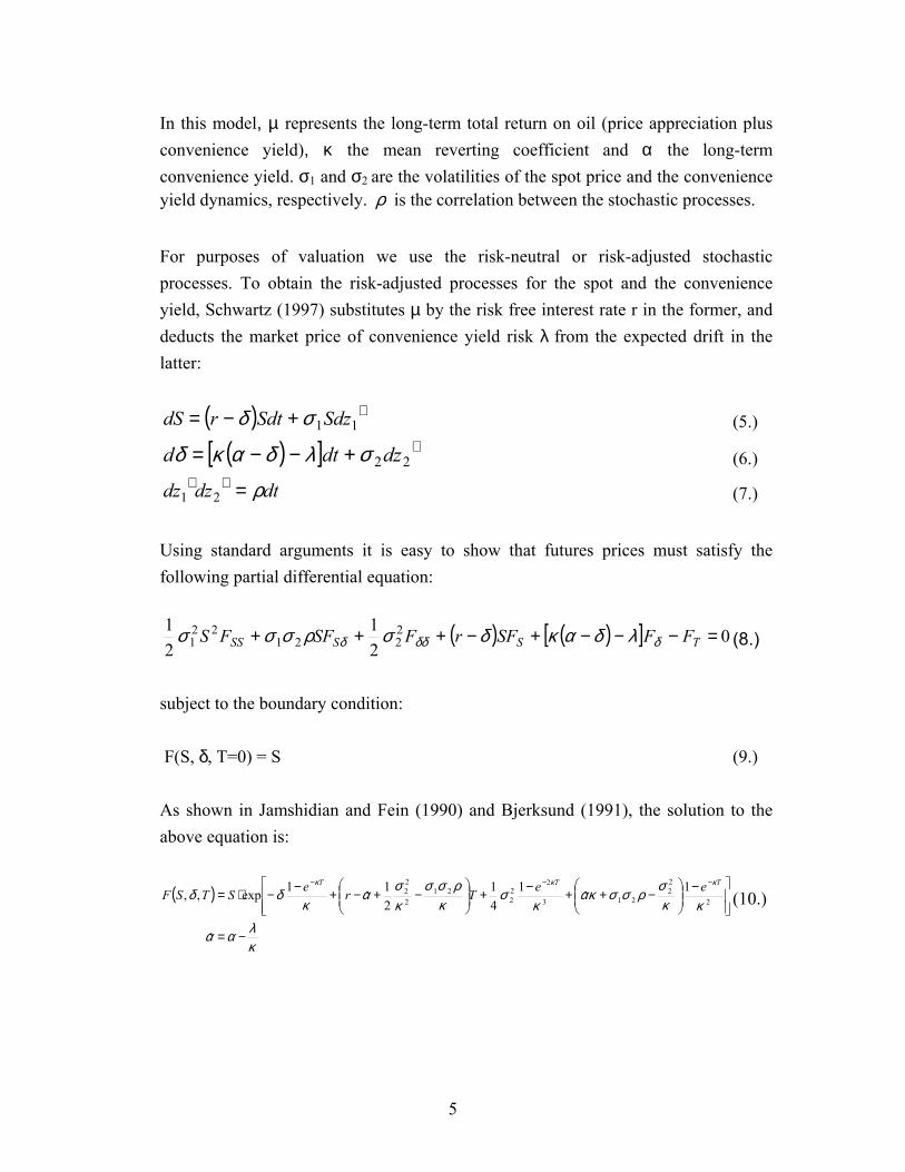
In this model, µ represents the long-term total return on oil (price appreciation plus convenience yield), κ the mean reverting coefficient and α the long-term convenience yield. σ1 and σ2 are the volatilities of the spot price and the convenience yield dynamics, respectively. ρ is the correlation between the stochastic processes.

For purposes of valuation we use the risk-neutral or risk-adjusted stochastic processes. To obtain the risk-adjusted processes for the spot and the convenience yield, Schwartz (1997) substitutes µ by the risk free interest rate r in the former, and deducts the market price of convenience yield risk λ from the expected drift in the latter:

( ) ∗+−= 11SdzSdtrdS σδ (5.)

( )[ ] ∗+−−= 22dzdtd σλδακδ (6.)

dtdzdz ρ=∗∗21 (7.)

Using standard arguments it is easy to show that futures prices must satisfy the following partial differential equation:

( ) ( )[ ] 021

21 2

22122

1 =−−−+−+++ TSSSS FFSFrFSFFS δδδδ λδακδσρσσσ (8.)

subject to the boundary condition: F(S, δ, T=0) = S (9.) As shown in Jamshidian and Fein (1990) and Bjerksund (1991), the solution to the above equation is:

( )

κλαα

κκσρσσκα

κσ

κρσσ

κσα

κδδ

κκκ

−=

−

−++−+

−+−+−−⋅=

−−−

ˆ

1ˆ

141

21

ˆ1exp,, 2

22

213

222

212

22

TTT eeTreSTSF (10.)

5

2.2 A Parsimonious Two-Factor Model In this section we modify the model described in the previous one to obtain a more -parsimonious representation of the two-factor model. This modification is essential for understanding the extension to a three-factor model we develop in the next section. A closer look at the Schwartz (1997) model shows that it can be rewritten in a simpler way with fewer parameters. We can define a new state variable y as the demeaned convenience yield δ by subtracting from it the long-term convenience yield α. y = δ − α (11.) We substitute Equation (11) in Equation (1) and define ν as the long-term price return (price appreciation) on oil obtained by deducting the long-term convenience yield α from the long term total return µ. That is: ν = µ − α (12.)

Equations (1) and (2) then become:

( ) 11SdzSdtydS σν +−= (13.)

22dzydtdy σκ +−= (14.)

In this formulation of the model we treat both factors S and y as non-traded state variables and, therefore, to transform the original processes ((13) and (14)) into the risk-adjusted processes we assign one risk premium to each process. Defining λ i as the risk premium associated with the factors, the risk-adjusted processes are:

( ) ∗+−−= 111 SdzSdtydS σλν (15.)

( ) ∗+−−= 222 dzdtydy σλκ (16.)

dtdzdz ρ=∗∗21 (17.)

6

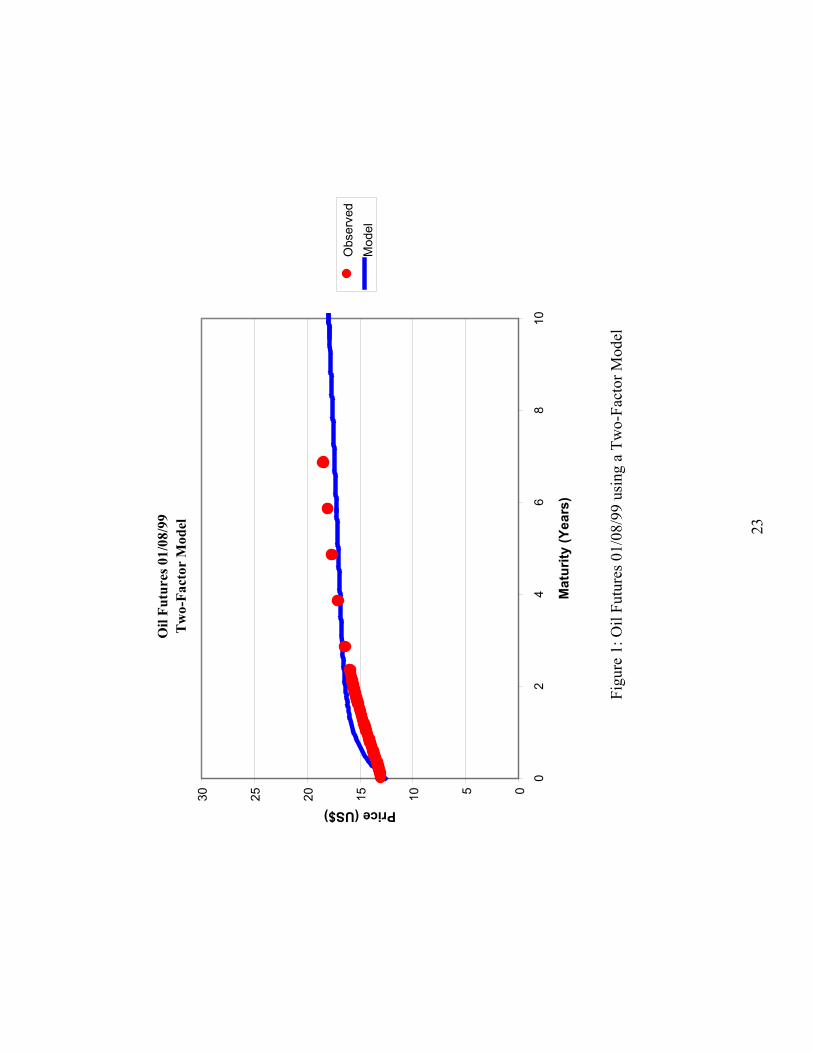
It must be stressed that this new model formulation, which has one parameter less than Schwartz (1997) has the same explanatory power but it is more parsimonious and is the basis of the three-factor model we develop later. Also with this formulation it becomes clear why Schwartz (1997) did not estimate the risk free interest rate from futures prices, but rather obtained it from bond data. Another benefit of this new formulation is that it is more intuitive for practitioner’s use. Returns are now defined in terms of the long-term price appreciation, which is more in line with industry practice than using the long-term convenience yield concept. We now turn to the explanatory power issue of the two-factor model. Even though Schwartz (1997) presents reasonable mean square errors when applying the two- factor model to a set of market prices, these averages hide the fact that for some days the model is unable to capture the behavior of market prices. This may be unacceptable for some model applications, such as its use to support trading. An example of a poor fit between market prices and the two-factor model is illustrated in Figure 1 by comparing model and observed market prices for oil futures traded at NYMEX on January 8th, 1999. The benefits of using the three-factor model described in the next section are illustrated in Figure 2, where we use it to explain the same market prices shown before, finding a remarkably better fit. This performance improvement, which may become important in many cases, is obtained without worsening the fitness for other dates for which the two-factor model behaved reasonably well. 2.3 A Three-Factor Model for Oil Prices. We now present the proposed three-factor model. We start with our reformulated version of the two-factor Schwartz (1997) model defining as state variables the commodity spot price, S, and the demeaned convenience yield, y. As in the two- factor model, the instantaneous expected spot price return is ν minus y and the expected long-term spot price return is ν. Thus y can also be defined as the deviation of spot price returns from its long-term value. This return deviation y is modeled as reverting with a coefficient k to its long-term value, which is by definition zero.

7

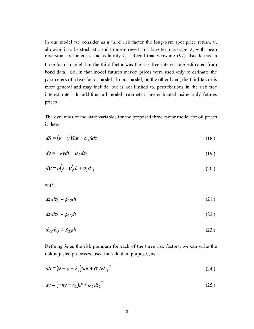
In our model we consider as a third risk factor the long-term spot price return, ν, allowing it to be stochastic and to mean revert to a long-term average ν , with mean reversion coefficient a and volatility 3σ . Recall that Schwartz (97) also defined a

three-factor model, but the third factor was the risk free interest rate estimated from bond data. So, in that model futures market prices were used only to estimate the parameters of a two-factor model. In our model, on the other hand, the third factor is more general and may include, but is not limited to, perturbations in the risk free interest rate. In addition, all model parameters are estimated using only futures prices. The dynamics of the state variables for the proposed three-factor model for oil prices is then:

( ) 11SdzSdtydS σν +−= (18.)

22dzydtdy σκ +−= (19.)

( ) 33dzdtad σννν +−= (20.)

with

dtdzdz 1221 ρ= (21.)

dtdzdz 1331 ρ= (22.)

dtdzdz 2332 ρ= (23.)

Defining λ i as the risk premium for each of the three risk factors, we can write the risk-adjusted processes, used for valuation purposes, as:

( ) ∗+−−= 111 SdzSdtydS σλν (24.)

( ) ∗+−−= 222 dzdtydy σλκ (25.)

8

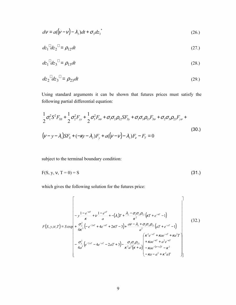
( ) *333)( dzdtad σλννν +−−= (26.)

dtdzdz 1221 ρ=∗∗ (27.)

dtdzdz 1331 ρ=∗∗ (28.)

dtdzdz 2332 ρ=∗∗ (29.)

Using standard arguments it can be shown that futures prices must satisfy the following partial differential equation:

( ) ( ) 0)()(

21

21

21

321

23321331122123

22

221

=−−−+−−+−−

++++++

TyS

ySSyyySS

FFaFySFy

FFSFFFFS

ν

νννν

λννλκλν

ρσσρσσρσσσσσ

(30.)

subject to the terminal boundary condition: F(S, y, ν, T = 0) = S (31.) which gives the following solution for the futures price:

( )

( ) ( )

( ) ( )

( ) ( ) ( )

+−−−−

++++

+−+−−−

−++−+−++−+

−+−+−+−+−−

=

+−

−−

−−

−−

−−−

−−

aTaaae

eaaeTaaee

aaaTee

a

eaTa

aTee

eTTaeey

STySF

Ta

TT

aTaT

aTaT

aTTT

TaTT

22

2

2

22

2223322

3

23

2133132

3

22

212212

1

3244

13244

111

exp,,,

κκκκ

κκκκ

κκρσσσ

ρσσλνκκ

σ

κκ

ρσσλλνκ

ν

κ

κκ

κκ

κκ

(32.)

9

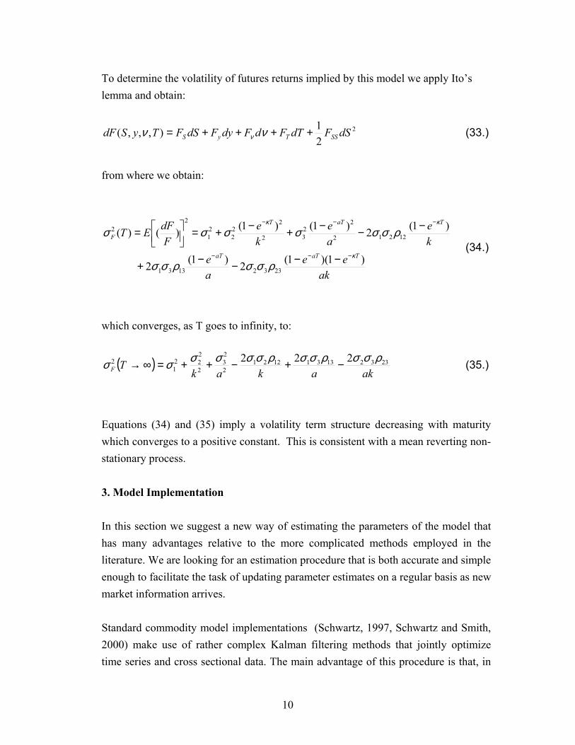
To determine the volatility of futures returns implied by this model we apply Ito’s lemma and obtain:

2

21),,,( dSFdTFdFdyFdSFTySdF SSTyS ++++= νν ν (33.)

from where we obtain:

akee

ae

ke

ae

ke

FdFET

TaTaT

TaTT

F

)1)(1(2)1(2

)1(2)1()1()()(

23321331

12212

2232

222

21

22

κ

κκ

ρσσρσσ

ρσσσσσσ

−−−

−−−

−−−−+

−−−+−+=

=

(34.)

which converges, as T goes to infinity, to:

( )akakak

TF233213311221

2

23

2

222

12 222 ρσσρσσρσσσσσσ −+−++=∞→ (35.)

Equations (34) and (35) imply a volatility term structure decreasing with maturity which converges to a positive constant. This is consistent with a mean reverting non-stationary process. 3. Model Implementation In this section we suggest a new way of estimating the parameters of the model that has many advantages relative to the more complicated methods employed in the literature. We are looking for an estimation procedure that is both accurate and simple enough to facilitate the task of updating parameter estimates on a regular basis as new market information arrives. Standard commodity model implementations (Schwartz, 1997, Schwartz and Smith, 2000) make use of rather complex Kalman filtering methods that jointly optimize time series and cross sectional data. The main advantage of this procedure is that, in

10

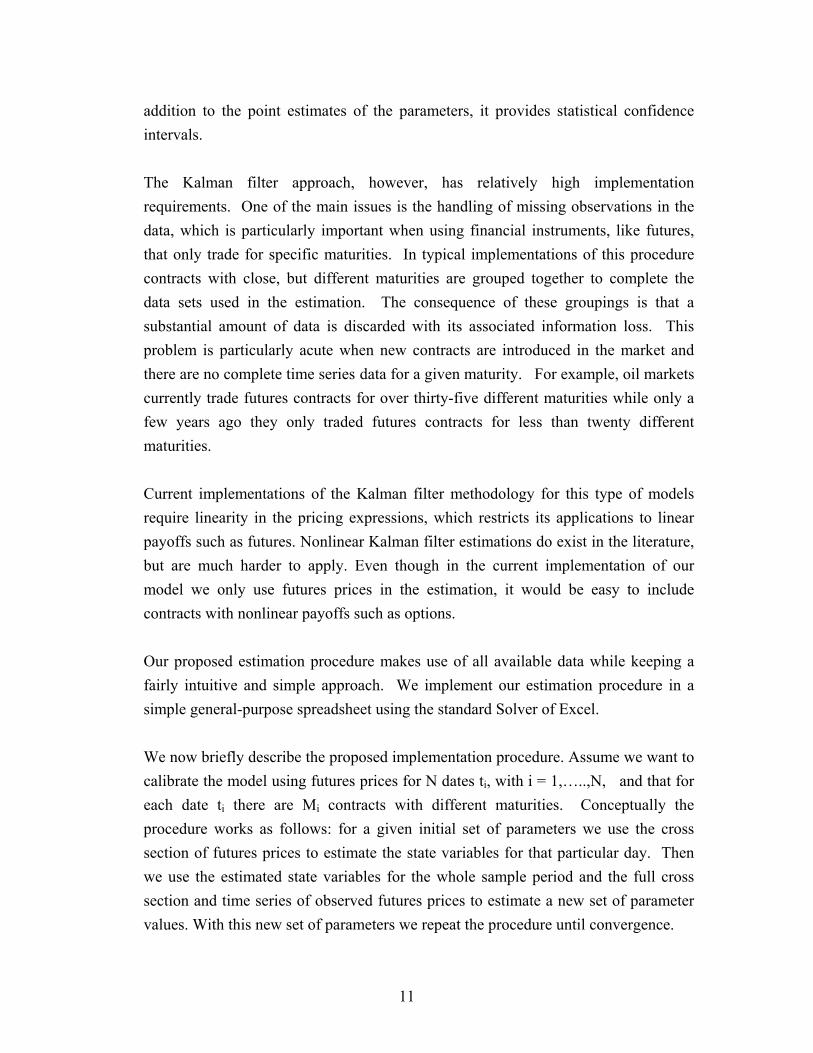
addition to the point estimates of the parameters, it provides statistical confidence intervals. The Kalman filter approach, however, has relatively high implementation requirements. One of the main issues is the handling of missing observations in the data, which is particularly important when using financial instruments, like futures, that only trade for specific maturities. In typical implementations of this procedure contracts with close, but different maturities are grouped together to complete the data sets used in the estimation. The consequence of these groupings is that a substantial amount of data is discarded with its associated information loss. This problem is particularly acute when new contracts are introduced in the market and there are no complete time series data for a given maturity. For example, oil markets currently trade futures contracts for over thirty-five different maturities while only a few years ago they only traded futures contracts for less than twenty different maturities. Current implementations of the Kalman filter methodology for this type of models require linearity in the pricing expressions, which restricts its applications to linear payoffs such as futures. Nonlinear Kalman filter estimations do exist in the literature, but are much harder to apply. Even though in the current implementation of our model we only use futures prices in the estimation, it would be easy to include contracts with nonlinear payoffs such as options. Our proposed estimation procedure makes use of all available data while keeping a fairly intuitive and simple approach. We implement our estimation procedure in a simple general-purpose spreadsheet using the standard Solver of Excel. We now briefly describe the proposed implementation procedure. Assume we want to calibrate the model using futures prices for N dates ti, with i = 1,…..,N, and that for each date ti there are Mi contracts with different maturities. Conceptually the procedure works as follows: for a given initial set of parameters we use the cross section of futures prices to estimate the state variables for that particular day. Then we use the estimated state variables for the whole sample period and the full cross section and time series of observed futures prices to estimate a new set of parameter values. With this new set of parameters we repeat the procedure until convergence.

11

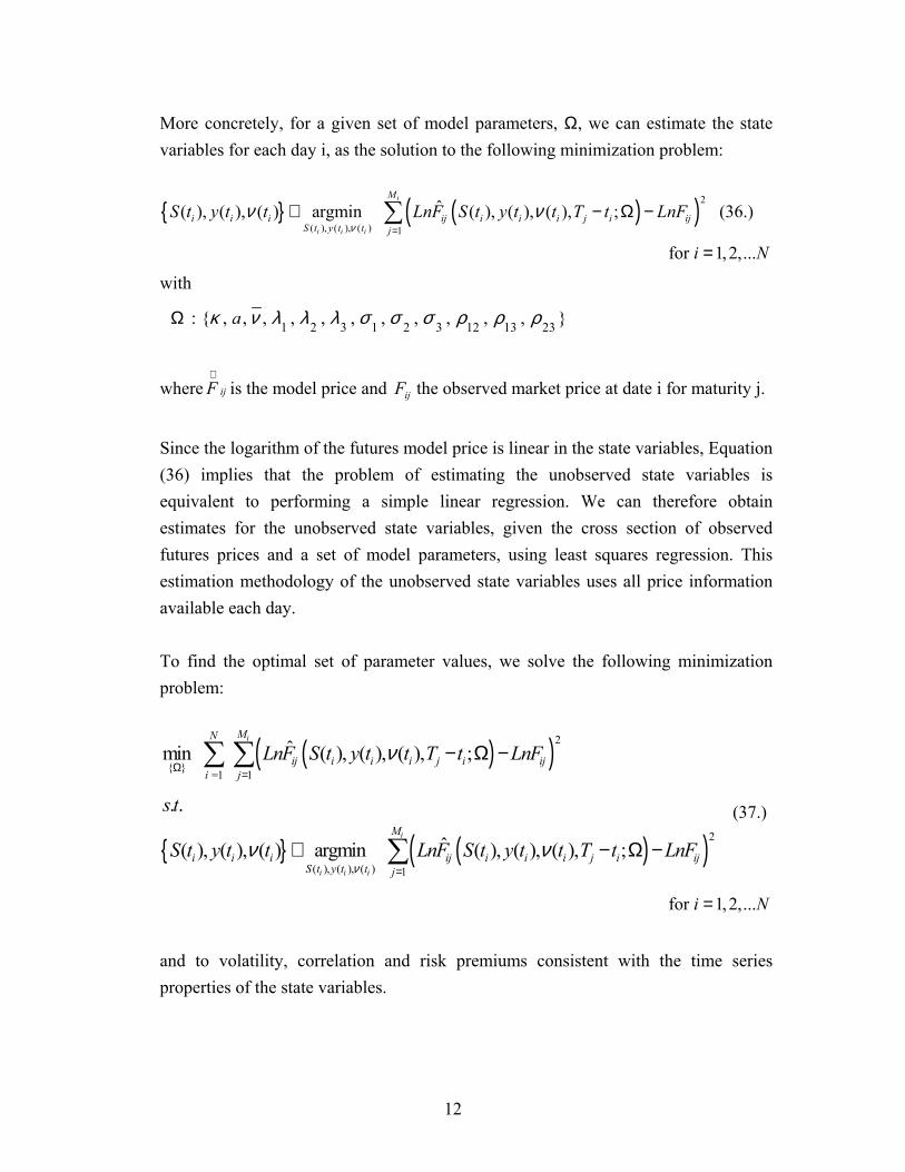
More concretely, for a given set of model parameters, Ω, we can estimate the state variables for each day i, as the solution to the following minimization problem:

( )( )2

( ), ( ), ( ) 1

ˆ( ), ( ), ( ) argmin ( ), ( ), ( ), ;i

i i i

M

i i i ij i i i j i ijS t y t t j

S t y t t LnF S t y t t T t LnFν

ν ν=

∈ −∑ Ω − (36.)

for 1, 2,...i N=

with

1 2 3 1 2 3 12 13 23: , , , , , , , , , , , aκ ν λ λ λ σ σ σ ρ ρ ρΩ

where is the model price and the observed market price at date i for maturity j. ijF∧

ijF

Since the logarithm of the futures model price is linear in the state variables, Equation (36) implies that the problem of estimating the unobserved state variables is equivalent to performing a simple linear regression. We can therefore obtain estimates for the unobserved state variables, given the cross section of observed futures prices and a set of model parameters, using least squares regression. This estimation methodology of the unobserved state variables uses all price information available each day. To find the optimal set of parameter values, we solve the following minimization problem:

( )( )

( )( )

2

=1 1

2

( ), ( ), ( ) 1

ˆmin ( ), ( ), ( ), ;

. .

ˆ( ), ( ), ( ) argmin ( ), ( ), ( ), ;

i

i

i i i

MN

ij i i i j i iji j

M

i i i ij i i i j i ijS t y t t j

LnF S t y t t T t LnF

s t

S t y t t LnF S t y t t T t LnFν

ν

ν ν

Ω =

=

− Ω −

∈ −

∑ ∑

∑ Ω −

(37.)

for 1, 2,...i N=

and to volatility, correlation and risk premiums consistent with the time series properties of the state variables.

12

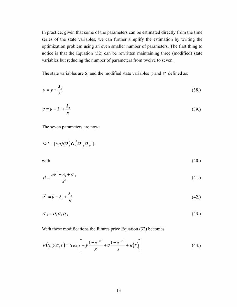
In practice, given that some of the parameters can be estimated directly from the time series of the state variables, we can further simplify the estimation by writing the optimization problem using an even smaller number of parameters. The first thing to notice is that the Equation (32) can be rewritten maintaining three (modified) state variables but reducing the number of parameters from twelve to seven. The state variables are S, and the modified state variables and y ν defined as:

κλ 2ˆ += yy (38.)

κλλνν 2

1ˆ +−= (39.)

The seven parameters are now:

2 2

2 3 12 23' : aκ βσ σ σ σΩ

with (40.)

2133

*

aa σλνβ +−= (41.)

κλλνν 2

1* +−= (42.)

133113 ρσσσ = (43.)

With these modifications the futures price Equation (32) becomes:

( ) ( )

+−+−−=

−−

TBaeeySTySF

aTT 1ˆ

1ˆexp,ˆ,ˆ, ν

κν

κ

(44.)

13

( ) ( )

( ) ( )

( ) ( ) ( )

−−−−

+++

++

+−+−−−

−++−++−+

−+−=

+−

−−

−−

−−

−−−

−

2

2

22

22

22232

3

23

23

22

212

3244

13244

1

aaae

eaaeaTTaaee

aaaTee

a

eaTTee

eTTB

Ta

TT

aTaT

aTaT

aTTT

T

κκκ

κκκκκ

κκσσ

βκκ

σ

κκσ

κ

κκ

κκ

κ

(45.)

The optimization problem then reduces to:

( )( )

( )( )

2

' =1 1

2

ˆˆ( ), ( ), ( ) 1

ˆ ˆˆmin ( ), ( ), ( ), ; '

. .

ˆˆ ˆˆ ˆ( ), ( ), ( ) argmin ( ), ( ), ( ), ; '

i

i

i i i

MN

ij i i i j i iji j

M

i i i ij i i i j i ijS t y t t j

LnF S t y t t T t LnF

s t

S t y t t LnF S t y t t T t LnFν

ν

ν ν

Ω =

=

− Ω −

∈ −

∑ ∑

∑ Ω −

(46.)

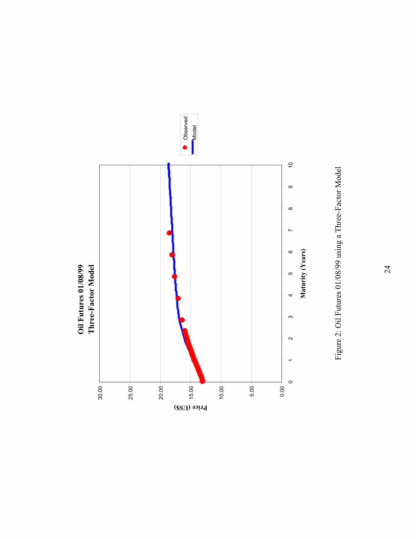
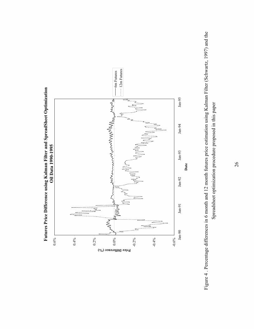
for 1, 2,...i N= and also subject to restrictions such that volatility and correlations are consistent with the time series properties of the state variables. This modification considerably simplifies the estimation procedure since we only have to estimate seven parameters. In what follows we will be using this modified model in all the calculations. The proposed procedure provides results reasonably close to those of the more formal Kalman filter estimation. For example, applying both estimation procedures to the weekly oil futures prices traded at NYMEX between 1990 and 1995 (similar to Panel B in Table 1 of Schwartz (1997)) we find very similar mean square errors (MSE). Figure 3 shows that the estimated values for the state variables are almost indistinguishable between the two procedures. Figure 4 shows that the percentage differences between the estimated values, using both procedures, for the six and twelve-month futures prices are very small and generally smaller than 0.5%.

14

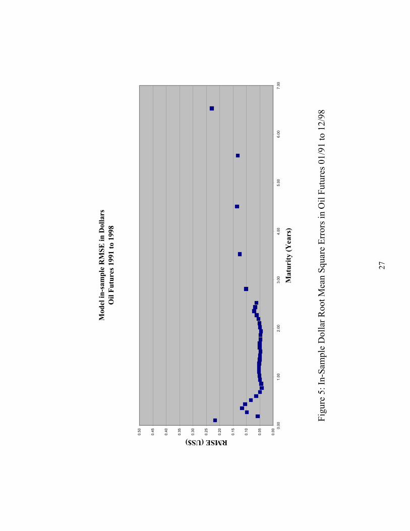
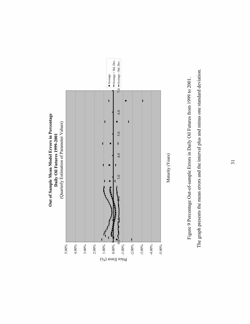
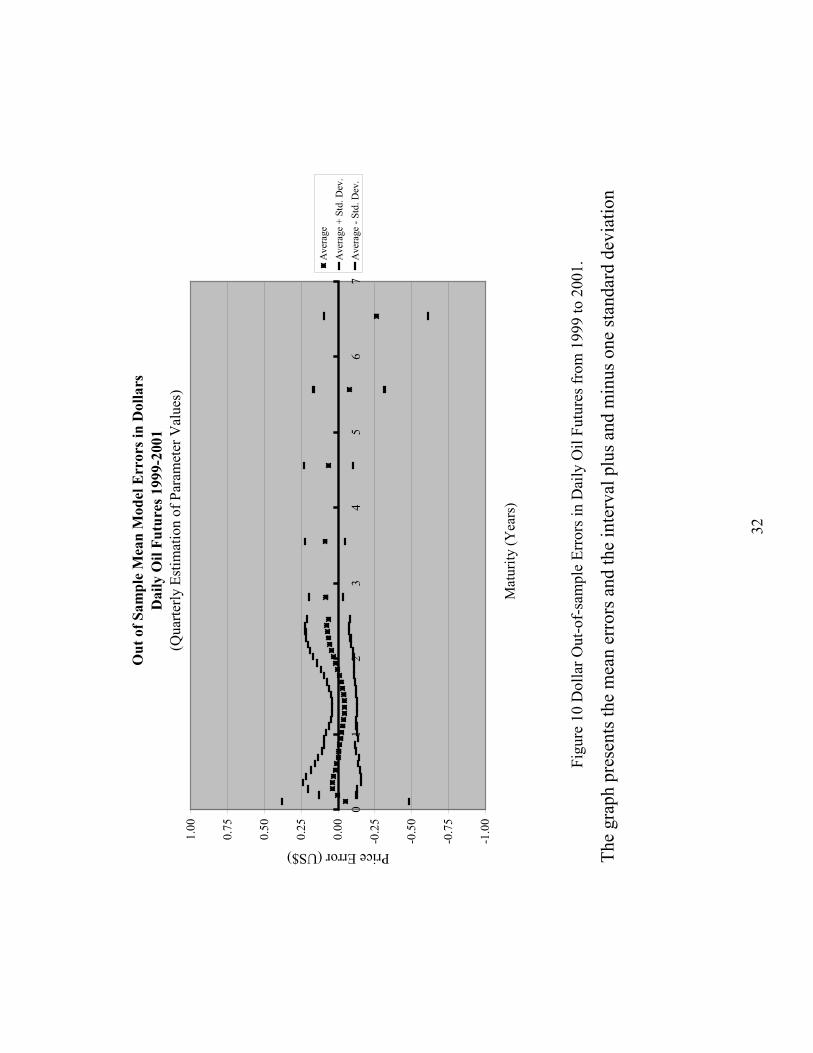
Even though this method has the disadvantage of not providing distributions for parameter estimates, its simplicity, accuracy, flexibility and easier use of the complete data set, makes it a valid alternative for many applications. 4. Results Having defined the model and the calibration procedure, we now present the results of applying it to recent oil futures price data. In this section we first define the data used, then we analyze in-sample model behavior, to finally show the results of applying the model to out-of-sample data. The data used are 76,121 daily prices corresponding to all futures contracts traded at the NYMEX from January 2nd 1991 to December 30th 2001. We do not aggregate data but use each available transaction separately. The number of different contracts traded each day at NYMEX has been increasing over the years, starting with 22 different contracts with a maximum maturity of 3 years, to end the sample period with 35 different contracts with maturity from 1 month to 7 years. Table 1 describes the futures data used. To test the model we split the data into two sets. Data-set 1 includes only transactions from January 2nd 1991 to December 30th 1998. We will use this data set to make our initial model calibration and to analyze the in-sample properties of our model. Data-set 2 includes the whole set from January 2nd 1991 to December 30th 2001, where the last three years will be used later to make the out-of-sample analysis of the model. Our in-sample results using Data-set 1 are reported in Figures 5 to 7. Figure 5 shows the dollar root mean square error (RMSE) between model and market prices across maturities. It can be seen that with the exceptions of the shortest and the longest maturity, the model estimates a futures price with a RMSE in the range of $0.05 - $0.15. Figure 6 presents the RMSE analysis in percentage terms across maturities. The average percentage RMSE is 0.42% and again it can be seen that the worse fit is for the shortest and the longest maturity contracts. All other contacts have a model RMSE between 0.25 and 0.75%.

15

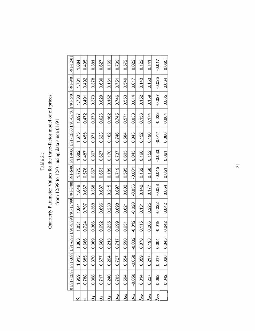
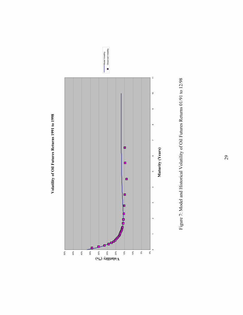
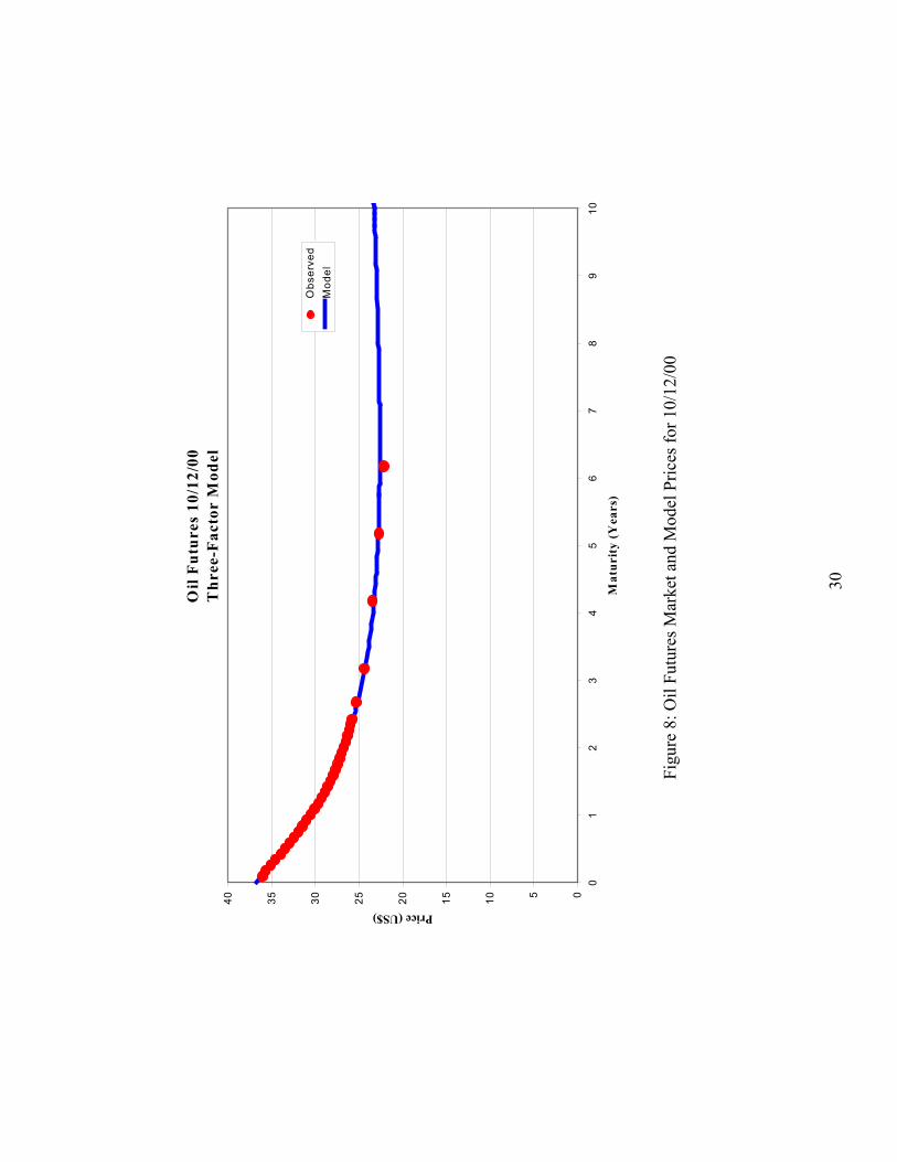
Figure 7 presents another measure of model goodness-of-fit by comparing the implied model volatility for different maturities with historical futures return volatility. Even though the model seems to exhibit a slight upward biased volatility for long-term contracts, it is remarkable how closely it tracks historical volatility for contracts with maturities up to 3 years. To make our out-of-sample analysis we use Data-set 2 and analyze the performance of the model over the last three years (1999 to 2001). Our initial model calibration, for transactions in the first quarter of 1999, is done with Data-set 1. The model is then recalibrated on a quarterly basis (on the last day of March, June, September and December of each year) and parameter values are not updated for the following three months. This out-of-sample analysis is done using only past information, available at the time of the calibration and represents an upper bound for the errors. More frequent calibrations could reduce model errors, since more recent prices would be included. Results for the three-year out-of-sample data are now presented. We start by noting that the model is very flexible in that it can deal with very different shapes of the term structure of futures prices. To illustrate this point we select arbitrary dates in the sample period in which futures oil prices exhibit either backwardation or contango. Figure 8 is representative of a day with a high degree of backwardation, while Figure 2 is an example of a day with prices that exhibit a strong contango. These figures are illustrations of how well the model may be used to explain very different term structures for oil futures prices. Table 2 provides the estimated quarterly parameter values from 12/98 to 12/01 for the three-factor model of oil prices. These results are obtained by solving the optimization problem for the parameters described earlier and by computing the volatility and correlation coefficients from the time series of state variables. Note that most of the parameters are quite stable over time. The only ones that are not stable are the risk premiums associated with the factors. These are the same parameters that turn to be statistically insignificant in the Kalman filter estimation (Schwartz, 1997). Using the parameter values in Table 2 we compute the out-of-sample model errors over the three-year period reported in what follows. Table 3 compares the RMSE (in

16

dollars and percentage) for both the in-sample and the out-of-sample data sets. As expected, the out-of-sample data set induces higher errors than the in-sample one, in this case by a factor of approximately two. Figures 9 and 10 plot the average errors and the one standard deviation interval of the futures out-of sample errors between 1999 and 2001 for different maturities. It can be seen that for most maturities the mean error is very close to zero and the standard deviation of the errors is less than 1% (or less than US$0.25). Note that these results were obtained recalibrating the model every quarter; obviously, more frequent parameter recalibration would increase even more the goodness-of-fit of the model. 4. Conclusions In this article we develop a parsimonious three-factor model of the term structure of futures oil prices, which fits the data extremely well. In addition, and very importantly, we propose an implementation procedure that significantly simplifies the estimation methods proposed in the literature. These factors make the proposed approach ideally suited for practical applications in the valuation and hedging of real and financial oil-contingent claims. The method can be used for other commodities as well; for example, we have also implemented the model using copper futures price data with similar results. The approach presented in the paper has been used in practice for almost three years to provide an estimate of the term structure of oil futures prices to an oil company. It is also currently used by the website www.riskamerica.com to provide daily estimates of the oil and copper futures curves. Acknowledgments This article is partially based on a working paper by Cortazar, Schwartz and Riera (2000). We would like to thank Fernando Riera who worked with us in the earlier stages of this project and Lorenzo Naranjo for excellent research assistance. This research was partially supported by a grant #D001024 from Fondef-Conicyt Chile.

17

References

BJERKSUND, P. (1991) "Contingent claims evaluation when the convenience yield is stochastic: Analytical results", Working Paper, Norwegian School of Economics and Business Administration.

BRENNAN, M.J. (1991) "The price of convenience and the valuation of commodity contingent claims", In D. Lund y B. Øksendal (eds.) Stochastic models and option values, Elsevier, North Holland.

BRENNAN, M.J. y SCHWARTZ, E.S. (1985) "Evaluating natural resources investments", Journal of Business, Vol. 58, N° 2, 135-157.

CORTAZAR, G. y SCHWARTZ, E.S. (1994) "The valuation of commodity-contingent claims", The Journal of Derivatives, Vol. 1, 27-35.

CORTAZAR, G. y SCHWARTZ, E.S. (1997) "Implementing a real option model for valuing an undeveloped oil field", International Transactions in Operational Research, Vol. 4, N° 2, 125-137.

CORTAZAR, G., SCHWARTZ, E., RIERA F. (2000) “Market-based Forecasts of Commodity Prices using Futures”, 4th Annual Conference Real Options: Theory Meets Practice International, Cambridge University/ROG Cambridge, July 7-8.

CULP, C.L. y MILLER, M.H. (1994) "Hedging a flow of commodity deliveries with futures: Lessons from Metallgesellschaft", Derivatives Quarterly, Vol. 1, N° 1, 7-15.

GIBSON, R. y SCHWARTZ, E.S. (1990) "Stochastic convenience yield and the pricing of oil contingent claims", The Journal of Finance, Vol. 45, N° 3, 959-976.

HEATH, D., JARROW, R. y MORTON, A. (1992) "Bond pricing and the term structure of interest rates: A new methodology for contingent claims valuation", Econometrica, Vol. 60, N° 4, 77-105.

JAMSHIDIAN, F. y FEIN, M. (1990) "Closed form solutions for oil futures and European options in the Gibson Schwartz model: A comment", Working Paper, Merrill Lynch Capital Markets.

LAUGHTON, D.G. y JACOBY, H.D. (1993) "Reversion, timing options, and long-term decision-making", Financial Management, Vol. 22, N° 3, 225-240.

18

LAUGHTON, D.G. y JACOBY, H.D. (1995) "The effects of reversion on commodity projects of different length", In L. Trigeorgis (ed.) Real options in capital investments: Models, strategies, and applications, Praeger Publisher, Westport, Conn.

PADDOCK, J., SIEGEL, D. y SMITH, J. (1988) "Option valuation of claims on real assets: The case of offshore petroleum leases", Quarterly Journal of Economics, Vol. 53, N° 3, 479-508.

SCHWARTZ, E.S. (1997) "The stochastic behavior of commodity prices: Implications for valuation and hedging", The Journal of Finance, Vol. 52, N° 3, 923-973.

SCHWARTZ, E.S. y SMITH, J.E. (2000) "Short-term variations and long-term dynamics in commodity prices", Management Science, Vol. 46, 893-911.

19

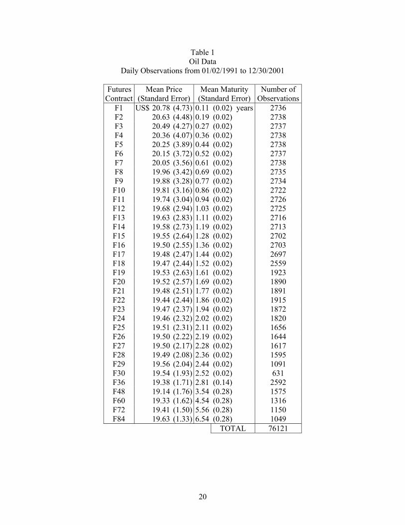
Table 1 Oil Data

Daily Observations from 01/02/1991 to 12/30/2001

Futures Contract

Mean Price (Standard Error)

Mean Maturity (Standard Error)

Number of Observations

F1 US$ 20.78 (4.73) 0.11 (0.02) years 2736 F2 20.63 (4.48) 0.19 (0.02) 2738 F3 20.49 (4.27) 0.27 (0.02) 2737 F4 20.36 (4.07) 0.36 (0.02) 2738 F5 20.25 (3.89) 0.44 (0.02) 2738 F6 20.15 (3.72) 0.52 (0.02) 2737 F7 20.05 (3.56) 0.61 (0.02) 2738 F8 19.96 (3.42) 0.69 (0.02) 2735 F9 19.88 (3.28) 0.77 (0.02) 2734 F10 19.81 (3.16) 0.86 (0.02) 2722 F11 19.74 (3.04) 0.94 (0.02) 2726 F12 19.68 (2.94) 1.03 (0.02) 2725 F13 19.63 (2.83) 1.11 (0.02) 2716 F14 19.58 (2.73) 1.19 (0.02) 2713 F15 19.55 (2.64) 1.28 (0.02) 2702 F16 19.50 (2.55) 1.36 (0.02) 2703 F17 19.48 (2.47) 1.44 (0.02) 2697 F18 19.47 (2.44) 1.52 (0.02) 2559 F19 19.53 (2.63) 1.61 (0.02) 1923 F20 19.52 (2.57) 1.69 (0.02) 1890 F21 19.48 (2.51) 1.77 (0.02) 1891 F22 19.44 (2.44) 1.86 (0.02) 1915 F23 19.47 (2.37) 1.94 (0.02) 1872 F24 19.46 (2.32) 2.02 (0.02) 1820 F25 19.51 (2.31) 2.11 (0.02) 1656 F26 19.50 (2.22) 2.19 (0.02) 1644 F27 19.50 (2.17) 2.28 (0.02) 1617 F28 19.49 (2.08) 2.36 (0.02) 1595 F29 19.56 (2.04) 2.44 (0.02) 1091 F30 19.54 (1.93) 2.52 (0.02) 631 F36 19.38 (1.71) 2.81 (0.14) 2592 F48 19.14 (1.76) 3.54 (0.28) 1575 F60 19.33 (1.62) 4.54 (0.28) 1316 F72 19.41 (1.50) 5.56 (0.28) 1150 F84 19.63 (1.33) 6.54 (0.28) 1049

TOTAL 76121

20

Tabl

e 2.

: Q

uarte

rly P

aram

eter

Val

ues f

or th

e th

ree-

fact

or m

odel

of o

il pr

ices

fr

om 1

2/98

to 1

2/01

usi

ng d

ata

sinc

e 01

/91

01

/91-

12/9

8 1/9

1-3/

99 1

/91-

6/99

1/9

1-9/

99 1

/91-

12/9

9 1/

91-3

/00

1/91

-6/0

01/

91-9

/00

1/91

-12/

00 1

/91-

03/0

1 1/

91-6

/01

1/91

-9/0

11/

91-1

2/01

Κ

1.95

9

1.

913

1.86

31.

831

1.84

11.

849

1.77

51.

682

1.67

51.

697

1.73

31.

731

1.68

4a

0.78

8

0.

685

0.68

60.

724

0.70

70.

667

0.57

80.

487

0.45

50.

472

0.49

10.

492

0.49

5

σ 1

0.36

8

0.

370

0.36

90.

366

0.36

80.

368

0.36

70.

367

0.37

10.

373

0.37

30.

378

0.38

1

σ 2

0.71

7

0.

677

0.68

00.

692

0.69

60.

687

0.65

30.

627

0.62

30.

626

0.62

90.

630

0.62

7

σ 3

0.24

0

0.

204

0.21

30.

235

0.23

00.

215

0.18

90.

170

0.16

20.

162

0.16

20.

161

0.16

9

ρ 12

0.70

5

0.

727

0.71

70.

699

0.69

80.

697

0.71

90.

737

0.74

60.

745

0.74

60.

751

0.73

9

ρ 23

0.59

4

0.

554

0.59

00.

631

0.62

10.

602

0.59

50.

603

0.58

40.

571

0.55

30.

549

0.57

2

ρ 13

-0.0

50

-0.0

58-0

.032

-0.0

12-0

.020

-0.0

36-0

.001

0.04

30.

043

0.03

30.

014

0.01

70.

022

λ 12

0.01

4

0.

059

0.07

80.

115

0.13

10.

142

0.16

20.

160

0.15

20.

156

0.15

20.

143

0.12

2

λ 23

0.22

7

0.

217

0.19

30.

206

0.22

50.

177

0.16

80.

152

0.19

00.

174

0.15

90.

153

0.14

1

λ 13

0.06

2

0.

017

0.00

4-0

.019

-0.0

22-0

.038

-0.0

45-0

.033

-0.0

17-0

.023

-0.0

27-0

.025

-0.0

17

0.04

2

0.

036

0.04

50.

042

0.04

20.

054

0.05

10.

061

0.06

00.

064

0.06

50.

064

0.06

5ν

21

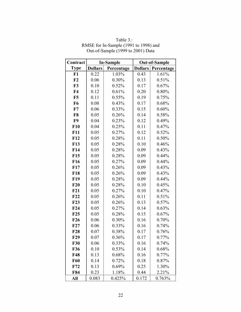
Table 3.:

RMSE for In-Sample (1991 to 1998) and Out-of-Sample (1999 to 2001) Data

In-Sample Out-of-Sample Contract

Type Dollars Percentage Dollars Percentage F1 0.22 1.03% 0.43 1.61% F2 0.06 0.30% 0.13 0.51% F3 0.10 0.52% 0.17 0.67% F4 0.12 0.61% 0.20 0.80% F5 0.11 0.55% 0.19 0.75% F6 0.08 0.43% 0.17 0.68% F7 0.06 0.33% 0.15 0.60% F8 0.05 0.26% 0.14 0.58% F9 0.04 0.23% 0.12 0.49% F10 0.04 0.25% 0.11 0.47% F11 0.05 0.27% 0.12 0.52% F12 0.05 0.28% 0.11 0.50% F13 0.05 0.28% 0.10 0.46% F14 0.05 0.28% 0.09 0.43% F15 0.05 0.28% 0.09 0.44% F16 0.05 0.27% 0.09 0.44% F17 0.05 0.26% 0.09 0.43% F18 0.05 0.26% 0.09 0.43% F19 0.05 0.28% 0.09 0.44% F20 0.05 0.28% 0.10 0.45% F21 0.05 0.27% 0.10 0.47% F22 0.05 0.26% 0.11 0.51% F23 0.05 0.26% 0.13 0.57% F24 0.05 0.27% 0.14 0.63% F25 0.05 0.28% 0.15 0.67% F26 0.06 0.30% 0.16 0.70% F27 0.06 0.33% 0.16 0.74% F28 0.07 0.38% 0.17 0.76% F29 0.07 0.36% 0.17 0.77% F30 0.06 0.33% 0.16 0.74% F36 0.10 0.53% 0.14 0.68% F48 0.13 0.68% 0.16 0.77% F60 0.14 0.72% 0.18 0.87% F72 0.13 0.69% 0.25 1.30% F84 0.23 1.18% 0.44 2.21%

All 0.083 0.425% 0.172 0.763%

22

Oil

Futu

res 0

1/08

/99

Tw

o-Fa

ctor

Mod

el

051015202530

02

46

810

Mat

urity

(Yea

rs)

Price (US$)

Obs

erve

dM

odel

Figu

re 1

: Oil

Futu

res 0

1/08

/99

usin

g a

Two-

Fact

or M

odel

23

Oil

Futu

res 0

1/08

/99

Thr

ee-F

acto

r M

odel

0.00

5.00

10.0

0

15.0

0

20.0

0

25.0

0

30.0

0

01

23

45

67

89

10

Mat

urity

(Yea

rs)

Price (US$)

Obs

erve

dM

odel

Fi

gure

2: O

il Fu

ture

s 01/

08/9

9 us

ing

a Th

ree-

Fact

or M

odel

24

Stat

e V

aria

bles

Val

ues u

sing

Kal

man

Filt

er a

nd S

prea

dShe

et O

ptim

izat

ion

Oil

Dat

a 19

90-1

995

1.5

2.0

2.5

3.0

3.5

4.0 Ja

n-90

Jan-

91Ja

n-92

Jan-

93Ja

n-94

Jan-

95

Dat

e

State Variables

Ln S

(SSh

eet)

Ln S

(Kal

man

)

Con

v.Y

ld+2

(Kal

man

)

Con

v.Y

ld+2

(SSh

eet)

Figu

re 3

. St

ate

varia

bles

val

ues o

f the

two-

fact

or m

odel

in S

chw

artz

(199

7) (L

og S

pot a

nd C

onve

nien

ce Y

ield

s) u

sing

Kal

man

Fi

lter a

nd o

ur sp

read

shee

t opt

imiz

atio

n pr

oced

ure

25

Futu

res P

rice

Diff

eren

ce u

sing

Kal

man

Filt

er a

nd S

prea

dShe

et O

ptim

izat

ion

Oil

Dat

a 19

90-1

995

-0.6

%

-0.4

%

-0.2

%

0.0%

0.2%

0.4%

0.6%

Jan-

90Ja

n-91

Jan-

92Ja

n-93

Jan-

94Ja

n-95

Dat

e

Price Difference (%)

6m F

utur

es12

m F

utur

es

Fi

gure

4 .

Perc

enta

ge d

iffer

ence

s in

6 m

onth

and

12

mon

th fu

ture

s pric

e es

timat

ion

usin

g K

alm

an F

ilter

(Sch

war

tz, 1

997)

and

the

Spre

adsh

eet o

ptim

izat

ion

proc

edur

e pr

opos

ed in

this

pap

er

26

Mod

el in

-sam

ple

RM

SE in

Dol

lars

Oil

Futu

res 1

991

to 1

998

0.00

0.05

0.10

0.15

0.20

0.25

0.30

0.35

0.40

0.45

0.50

0.00

1.00

2.00

3.00

4.00

5.00

6.00

7.00

Mat

urity

(Yea

rs)

RMSE (US$)

Figu

re 5

: In-

Sam

ple

Dol

lar R

oot M

ean

Squa

re E

rror

s in

Oil

Futu

res 0

1/91

to 1

2/98

27

Mod

el in

-sam

ple

RM

SE in

Per

cent

ages

Oil

Futu

res 1

991

to 1

998

0.00

%

0.25

%

0.50

%

0.75

%

1.00

%

1.25

%

1.50

%

1.75

%

2.00

%

2.25

%

2.50

% 0.00

1.00

2.00

3.00

4.00

5.00

6.00

7.00

Mat

urity

(Yea

rs)

RMSE (%)

Fi

gure

6: I

n-Sa

mpl

e Pe

rcen

tage

Roo

t Mea

n Sq

uare

Err

ors i

n O

il Fu

ture

s 01/

91 to

12/

98

28

Vol

atili

ty o

f Oil

Futu

res R

etur

ns 1

991

to 1

998

0%5%10%

15%

20%

25%

30%

35%

40%

45%

50%

01

23

45

67

89

1011

Mat

urity

(Yea

rs)

Volatility (%)

Mod

el V

olat

ility

Obs

erve

d Vo

latil

ity

Figu

re 7

: Mod

el a

nd H

isto

rical

Vol

atili

ty o

f Oil

Futu

res R

etur

ns 0

1/91

to 1

2/98

29

Oil

Fut

ures

10/

12/0

0T

hree

-Fac

tor

Mod

el

0510152025303540

01

23

45

67

89

10

Mat

urit

y (Y

ears

)

Price (US$)

Obs

erve

dM

odel

Figu

re 8

: Oil

Futu

res M

arke

t and

Mod

el P

rices

for 1

0/12

/00

30

Out

of S

ampl

e M

ean

Mod

el E

rror

s in

Perc

enta

geD

aily

Oil

Futu

res 1

999-

2001

(Qua

rterly

Est

imat

ion

of P

aram

eter

Val

ues)

-5.0

0%

-4.0

0%

-3.0

0%

-2.0

0%

-1.0

0%

0.00

%

1.00

%

2.00

%

3.00

%

4.00

%

5.00

%

0.0

1.0

2.0

3.0

4.0

5.0

6.0

7.0

Mat

urity

(Yea

rs)

Price Error (%)

Ave

rage

Ave

rage

+ S

td. D

ev.

Ave

rage

- St

d. D

ev.

Figu

re 9

Per

cent

age

Out

-of-

sam

ple

Erro

rs in

Dai

ly O

il Fu

ture

s fro

m 1

999

to 2

001.

The

grap

h pr

esen

ts th

e m

ean

erro

rs a

nd th

e in

terv

al p

lus a

nd m

inus

one

stan

dard

dev

iatio

n.

31

Out

of S

ampl

e M

ean

Mod

el E

rror

s in

Dol

lars

Dai

ly O

il Fu

ture

s 199

9-20

01(Q

uarte

rly E

stim

atio

n of

Par

amet

er V

alue

s)

-1.0

0

-0.7

5

-0.5

0

-0.2

5

0.00

0.25

0.50

0.75

1.00

01

23

45

67

Mat

urity

(Yea

rs)

Price Error (US$)

Ave

rage

Ave

rage

+ S

td. D

ev.

Ave

rage

- St

d. D

ev.

Figu

re 1

0 D

olla

r Out

-of-

sam

ple

Erro

rs in

Dai

ly O

il Fu

ture

s fro

m 1

999

to 2

001.

The

grap

h pr

esen

ts th

e m

ean

erro

rs a

nd th

e in

terv

al p

lus a

nd m

inus

one

stan

dard

dev

iatio

n

32