Implementing Quotas in GTAP usingGEMPACK or

How to Linearize an Inequality

Christian F. Bach and K. R. Pearson

GTAP Technical Paper No. 4

8 November 1996

Christian F. Bach, Institute of Economics, University of Copenhagen, Studiestraede 6, DK-1455 CopenhagenK, Denmark. Email: okocfb@pc.ibt.dk

Ken Pearson, Centre of Policy Studies and Impact Project, Monash University, Clayton Vic 3168, Australiaand Department of Mathematics, La Trobe University. Email: Ken.Pearson@BusEco.monash.edu.au

GTAP stands for the Global Trade Analysis Project which is administered by the Center for Global TradeAnalysis, Purdue University, West Lafayette, Indiana, USA 47907-1145. For more information about GTAP,please refer to our Worldwide Web site at: http://www.agecon.purdue.edu/gtap/, or send a request toconner@agecon.purdue.edu

Implementing Quotas in GTAP using GEMPACKor How to Linearize an Inequality

Abstract

This document describes how explicit import and export quotas can beimplemented and solved in the GTAP CGE trade model. Thetechniques described here apply equally well to other general and partialequilibrium models implemented and solved using the GEMPACKsoftware. They also generalize to procedures for handling otherinequalities in models solved via GEMPACK (even though GEMPACKdoes not allow explicit inequalities in the algebraic representation ofmodels).

This document describes some recent applications of GTAP in whichexplicit import and export quotas have been modelled, and discusseshow important it was for these applications to have explicit quotasmodelled.

Accompanying this document are various computer files containing theingredients of examples that readers can carry out for themselves whilereading this paper. These files can also be used as a starting point forthose who wish to explicitly model quotas in their own models.

ii

Table of Contents

1. Introduction...................................................................................................................................1

1.1 Bilateral Quotas - The Basic Idea ............................................................................................2GTAP Notation..........................................................................................................................3

2. Bilateral Export Quotas.................................................................................................................4

2.1 Results of this MFA Application ..............................................................................................8

3. Implementing Bilateral Export Quotas in GTAP ............................................................................9

3.1 Implementation as Additions/Modifications to GTAP.TAB ......................................................9

3.2 Quota Rents ..........................................................................................................................10

3.3 TABLO Statements for Export Quotas ..................................................................................11

3.4 Assigning Initial QXS_RATIO_L and VXQD Values............................................................11

3.5 Closures for the Model ..........................................................................................................12

3.6 Accurate Export Quota Solutions ..........................................................................................123.6.1 Checking the Accurate Simulation ..................................................................................14

4. Export Quotas in a 3x3 Version of GTAP....................................................................................14

5. Bilateral Import Quotas ...............................................................................................................15

5.1 Import Quota Variables and Equations ..................................................................................16

5.2 Calibrating VIQS and QIS_RATIO_L Values for this Application.........................................17

5.3 Results of this Application.....................................................................................................18

6. Bilateral Import Quotas in GTAP ................................................................................................19

6.1 Implementation as Additions/Modifications to GTAP.TAB ....................................................20

6.2 Quota rents ...........................................................................................................................21

6.3 TABLO Statements for Import Quotas ..................................................................................21

6.4 Assigning Initial QIS_RATIO_L and VIQS Values ...............................................................21

iii

6.5 Closures for the Model ..........................................................................................................22

6.6 Accurate Import Quota Solutions...........................................................................................226.6.1 Checking the Accurate Simulation ..................................................................................23

7. Import Quotas in a 3x3 Version of GTAP....................................................................................24

8. Automating the Second Part of the Two-Part Solution Procedure..................................................25

8.1 Automating the Shocks..........................................................................................................25

8.2 Automating the Closure Change.............................................................................................26

8.3 Automating Shocks and Closure Swaps with Release 5.2 of GEMPACK ...............................26

8.4 An Alternative Closure for the Accurate Simulation...............................................................27

9. Handling Other Inequalities using GEMPACK.............................................................................28Kuhn-Tucker Conditions..........................................................................................................28Non-negative Investment ..........................................................................................................29Other Quotas ...........................................................................................................................29

10. Conclusion ................................................................................................................................29

11. References.................................................................................................................................30

Appendix 1: Installing and Using the Associated Files ......................................................................31Obtaining QUOTA-EX.ZIP and/or the Demonstration Version of GEMPACK ......................31

Appendix 2: Additions to GTAP94.TAB for Bilateral Export Quotas...............................................32

Appendix 3: Linearizing the Exp_Quo_Ratios Levels Equations for Quotas.....................................35Linearizing MAX(QR,PR)=1 ...................................................................................................35Linearizing MAX(QR,PR)=1 with Newton Correction..............................................................36

Implementing Quotas in GTAP usingGEMPACK -or How to Linearize an

Inequality

1. Introduction

Quantitative trade restrictions have been implemented in a number of Computable GeneralEquilibrium models. However, modellers from the linearized school (that is, those workingwith a linearized representation of the equations of their model) have been reluctant to movetowards explicit modelling of quota constraints as this inevitably requires implementing aninequality in a linearized representation. This technical paper demonstrates how theseproblems can be overcome, and how quotas can prove useful in a number of everyday policyproblems. Binding volume quotas are introduced in the GTAP model [Hertel, 1996] andsolved via a linearized representation using GEMPACK [Harrison and Pearson, 1994].

In section 2 we introduce the policy problem which spurred the current formulation of bilateralexport quotas in GTAP, and present the levels versions of the export quota equations. Insection 3 we take a detailed look on the actual implementation of bilateral export quotas in theGTAP model (which is implemented via a linearized representation). In section 4 we tell youhow you can work through several examples of simulations involving bilateral export quotaswith a 3-commodity, 3-region version of GTAP. These sections are subsequently replicatedbut with bilateral import quotas in sections 5, 6 and 7. Solving a model with quotas viaGEMPACK involves a two-part process (as explained in the examples in sections 3.6 and 6.6).Ways of automating the second part of this process are described in section 8. In section 9 webriefly discuss ways in which other inequalities can be modelled using GEMPACK. In section10 we make a few concluding remarks. Section 11 contains references.

Some more technical material is presented in the various appendices. In Appendix 1 we tellyou how you can install and use the computer files associated with this document on your PC.You can then carry out the examples as you read this document. Appendix 2 contains theTABLO statements which are added to the standard TABLO Input file GTAP94.TAB forGTAP to implement bilateral export quotas. Appendix 3 contains the details of thelinearization of the key levels equation used to describe quotas.

Quotas and other inequalities can, of course, also be modelled directly using other software,including GAMS [Brooke, 1988] and GAMS/MPSGE [Rutherford, 1995].

2

We assume that readers of this document are familiar with the standard computer version ofthe GTAP model [as documented in Hertel, 1996] and are also familiar with the procedure forimplementing and solving models using GEMPACK [Harrison and Pearson, 1994]. Inparticular we frequently use notation from the TABLO Input file GTAP94.TAB for GTAPwithout explicit cross referencing.

We are grateful to Mark Horridge who worked out the procedures described here for handlinginequalities using GEMPACK [Horridge, 1993]. We are also grateful to Jill Harrison, TomHertel and Michael Malakellis for helpful discussions about various aspects of this paper.

1.1 Bilateral Quotas - The Basic Idea

In this section we introduce the essential concepts involved in the way we have modelledexplicit bilateral export and import quotas, and also introduce the corresponding relevantGTAP notation for those not familiar with GTAP.

Consider exports of some commodity, say food, from one region, say USA, to another region,say the European Union EU. Firstly there is the volume exported, say QXS. Clearly thevolume of USA food exported to the EU is the same as the volume of food from the USAimported into EU.

There are several prices associated with this volume. Firstly there is

PM the basic or market price in the exporting region(this is usually the cost of producing the commodity)

There may be export taxes or subsidies added to this to give

PXS the price including export taxes or subsidies

[If there are taxes, PXS > PM while PXS < PM if there are subsidies.] Then there is

PFOB the f.o.b. price

Without export quotas, PFOB=PXS. But if there is a binding export quota we expect PFOBto be larger than PXS.

Then this volume is transported to the importing region where we have

PCIF the c.i.f. import price

3

PCIF has costs such as freight and insurance added to PFOB. There may be import tariffs orsubsidies added to this to give

PIS the price of imports including any import tariff or subsidy (butnot including the tariff equivalent of any quota)

There is also

PMS the basic or market price in the importing region

Without import quotas, PIS=PMS. But if there is a binding import quota we expect PMS to belarger than PIS.

With this notation, we have

PXS <= PFOBPFOB = PXS if the quota is not bindingPFOB > PXS if the quota is binding

PMS >= PISPMS = PIS if the quota is not bindingPMS > PIS if the quota is binding

We consider the export quota responsible for any difference between PXS and PFOB and theimport quota responsible for any difference between PIS and PMS. These simple ideas are thekey to our implementation of these quotas.

GTAP Notation

Above we have used the usual GTAP notation for those prices which exist in standard GTAP(that is, the standard version without export or import quotas). The prices denoted above byPXS and PIS are not present in the standard GTAP model since there PXS=PFOB andPIS=PMS. Of course each of the above prices really needs indices after it to account for thedifferent commodities, exporting and importing regions in the model: thus we really should bewriting PM(i,r), PXS(i,r,s), PFOB(i,r,s) etc.

4

The table below summarises these different prices and their associated values in GTAP.

GTAP price GTAP valuePM(i,r) VXMD(i,r,s)

] Differences due to "normal" export taxes/subsidiesPXS(i,r,s) VXQD(i,r,s)

] Differences due to export quotasPFOB(i,r,s) VXWD(i,r,s)

] Differences due to transport costs, insurance etcPCIF(i,r,s) VIWS(i,r,s)

] Differences due to "normal" import tariffs/subsidiesPIS(i,r,s) VIQS(i,r,s)

] Differences due to import quotasPMS(i,r,s) VIMS(i,r,s)

2. Bilateral Export Quotas

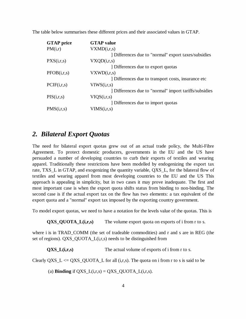
The need for bilateral export quotas grew out of an actual trade policy, the Multi-FibreAgreement. To protect domestic producers, governments in the EU and the US havepersuaded a number of developing countries to curb their exports of textiles and wearingapparel. Traditionally these restrictions have been modelled by endogenizing the export taxrate, TXS_L in GTAP, and exogenizing the quantity variable, QXS_L, for the bilateral flow oftextiles and wearing apparel from most developing countries to the EU and the US Thisapproach is appealing in simplicity, but in two cases it may prove inadequate. The first andmost important case is when the export quota shifts status from binding to non-binding. Thesecond case is if the actual export tax on the flow has two elements: a tax equivalent of theexport quota and a "normal" export tax imposed by the exporting country government.

To model export quotas, we need to have a notation for the levels value of the quotas. This is

QXS_QUOTA_L(i,r,s) The volume export quota on exports of i from r to s.

where i is in TRAD_COMM (the set of tradeable commodities) and r and s are in REG (theset of regions). QXS_QUOTA_L(i,r,s) needs to be distinguished from

QXS_L(i,r,s) The actual volume of exports of i from r to s.

Clearly QXS_L <= QXS_QUOTA_L for all (i,r,s). The quota on i from r to s is said to be

(a) Binding if QXS_L(i,r,s) = QXS_QUOTA_L(i,r,s).

5

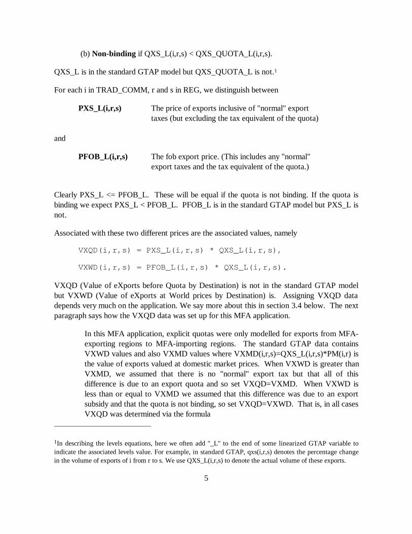
(b) Non-binding if QXS_L(i,r,s) < QXS_QUOTA_L(i,r,s).

QXS_L is in the standard GTAP model but QXS_QUOTA_L is not.1

For each i in TRAD_COMM, r and s in REG, we distinguish between

PXS_L(i,r,s) The price of exports inclusive of "normal" exporttaxes (but excluding the tax equivalent of the quota)

and

PFOB_L(i,r,s) The fob export price. (This includes any "normal"export taxes and the tax equivalent of the quota.)

Clearly PXS_L <= PFOB_L. These will be equal if the quota is not binding. If the quota isbinding we expect PXS_L < PFOB_L. PFOB_L is in the standard GTAP model but PXS_L isnot.

Associated with these two different prices are the associated values, namely

VXQD(i,r,s) = PXS_L(i,r,s) * QXS_L(i,r,s),

VXWD(i,r,s) = PFOB_L(i,r,s) * QXS_L(i,r,s).

VXQD (Value of eXports before Quota by Destination) is not in the standard GTAP modelbut VXWD (Value of eXports at World prices by Destination) is. Assigning VXQD datadepends very much on the application. We say more about this in section 3.4 below. The nextparagraph says how the VXQD data was set up for this MFA application.

In this MFA application, explicit quotas were only modelled for exports from MFA-exporting regions to MFA-importing regions. The standard GTAP data containsVXWD values and also VXMD values where VXMD(i,r,s)=QXS_L(i,r,s)*PM(i,r) isthe value of exports valued at domestic market prices. When VXWD is greater thanVXMD, we assumed that there is no "normal" export tax but that all of thisdifference is due to an export quota and so set VXQD=VXMD. When VXWD isless than or equal to VXMD we assumed that this difference was due to an exportsubsidy and that the quota is not binding, so set VXQD=VXWD. That is, in all casesVXQD was determined via the formula

1In describing the levels equations, here we often add "_L" to the end of some linearized GTAP variable toindicate the associated levels value. For example, in standard GTAP, qxs(i,r,s) denotes the percentage changein the volume of exports of i from r to s. We use QXS_L(i,r,s) to denote the actual volume of these exports.

6

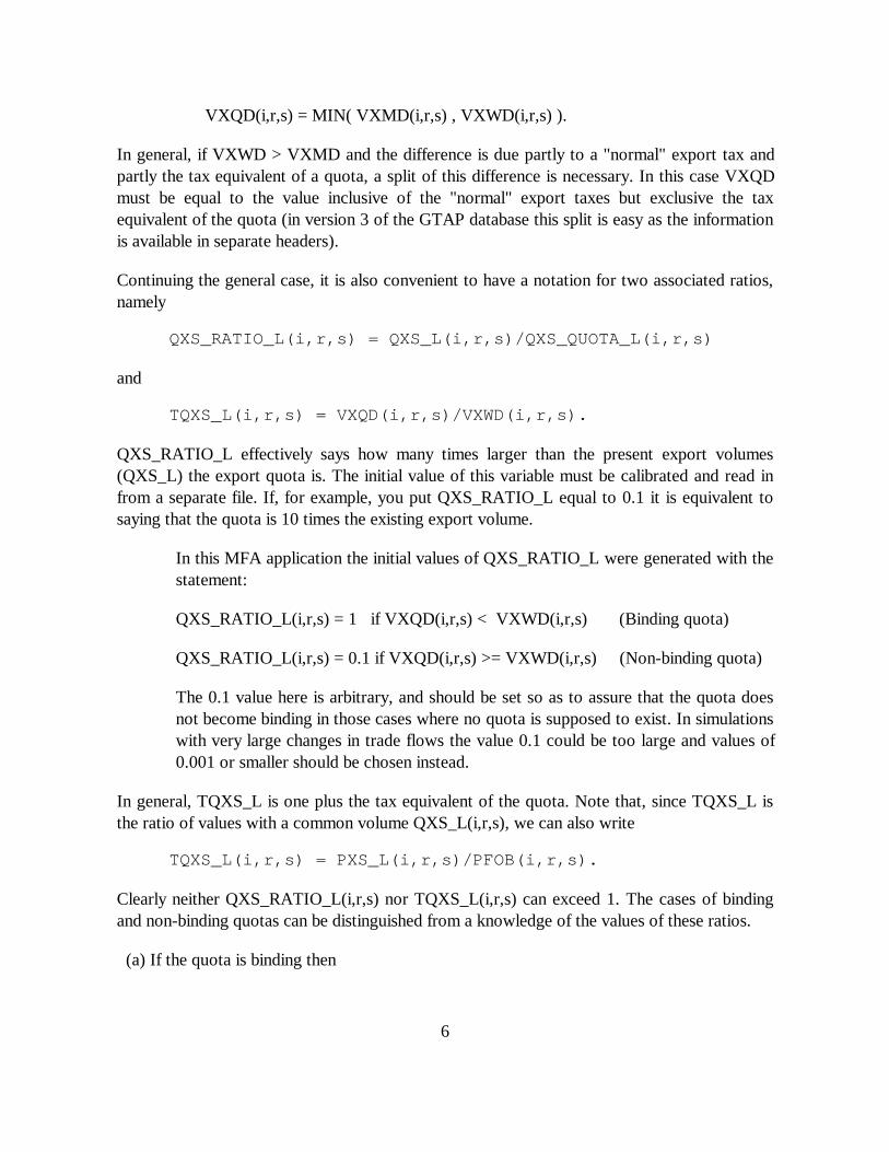
VXQD(i,r,s) = MIN( VXMD(i,r,s) , VXWD(i,r,s) ).

In general, if VXWD > VXMD and the difference is due partly to a "normal" export tax andpartly the tax equivalent of a quota, a split of this difference is necessary. In this case VXQDmust be equal to the value inclusive of the "normal" export taxes but exclusive the taxequivalent of the quota (in version 3 of the GTAP database this split is easy as the informationis available in separate headers).

Continuing the general case, it is also convenient to have a notation for two associated ratios,namely

QXS_RATIO_L(i,r,s) = QXS_L(i,r,s)/QXS_QUOTA_L(i,r,s)

and

TQXS_L(i,r,s) = VXQD(i,r,s)/VXWD(i,r,s).

QXS_RATIO_L effectively says how many times larger than the present export volumes(QXS_L) the export quota is. The initial value of this variable must be calibrated and read infrom a separate file. If, for example, you put QXS_RATIO_L equal to 0.1 it is equivalent tosaying that the quota is 10 times the existing export volume.

In this MFA application the initial values of QXS_RATIO_L were generated with thestatement:

QXS_RATIO_L(i,r,s) = 1 if VXQD(i,r,s) < VXWD(i,r,s) (Binding quota)

QXS_RATIO_L(i,r,s) = 0.1 if VXQD(i,r,s) >= VXWD(i,r,s) (Non-binding quota)

The 0.1 value here is arbitrary, and should be set so as to assure that the quota doesnot become binding in those cases where no quota is supposed to exist. In simulationswith very large changes in trade flows the value 0.1 could be too large and values of0.001 or smaller should be chosen instead.

In general, TQXS_L is one plus the tax equivalent of the quota. Note that, since TQXS_L isthe ratio of values with a common volume QXS_L(i,r,s), we can also write

TQXS_L(i,r,s) = PXS_L(i,r,s)/PFOB(i,r,s).

Clearly neither QXS_RATIO_L(i,r,s) nor TQXS_L(i,r,s) can exceed 1. The cases of bindingand non-binding quotas can be distinguished from a knowledge of the values of these ratios.

(a) If the quota is binding then

7

QXS_RATIO_L=1 and TQXS_L <= 1 (usually TQXS_L < 1).

This is because QXS_L = QXS_QUOTA_L and PXS_L <= PFOB_L (and usually PXS_L < PFOB_L).

(b) If the quota is not binding then

QXS_RATIO < 1 and TQXS_L = 1.

This is because QXS_L < QXS_QUOTA_L and PXS_L = PFOB_L.

This introduces the important equation

MAX [ QXS_RATIO(i,r,s), TQXS_L(i,r,s) ] = 1 for all (i,r,s).

This equation says that, for each (i,r,s), the maximum of these two ratios must equal 1. Sinceeach ratio is at most one, one of the two ratios must equal 1 for each (i,r,s). (Usually the otheris less than 1.)

To summarize, the main new levels variables are,

QXS_QUOTA_L, PXS_L, QXS_RATIO_L, TQXS_L, VXQD.

Of these, usually QXS_QUOTA_L is exogenous and the rest are endogenous. The new levelsequations are

QXS_RATIO_L(i,r,s) = QXS_L(i,r,s)/QXS_QUOTA_L(i,r,s) (L1)

TQXS_L(i,r,s) = PXS_L(i,r,s)/PFOB(i,r,s) (L2)

VXQD(i,r,s) = PXS_L(i,r,s) * QXS_L(i,r,s) (L3)

MAX [ QXS_RATIO_L(i,r,s), TQXS_L(i,r,s) ] = 1 (L4 )

As you can see, there are 5 lots of new levels variables and 4 lots of new levels equations. Thisis consistent with just one lot of these (usually the QXS_QUOTA_L values) being setexogenously. The model should then determine the rest of these.

It is equation L4 above which causes the problems for GEMPACK whose solution algorithmsare not well suited to handling such non-smooth levels equations. We refer to this equation bythe name Exp_Quo_Ratios, which is the name given to the associated linearized version inthe TABLO Input file GTAP33XQ.TAB as set out in Appendix 2.

In addition to the above new equations the equation EXPRICES connecting the fob price ofexports pfob(i,r,s) to the domestic price pm(i,r) and "normal" export taxes tx(i,r) and txs(i,r,s)

8

must now be rewritten. It now connects, in the levels, PXS_L(i,r,s) to these rather thanPFOB_L(i,r,s). Thus the levels equation previously in the model, namely

PFOB_L(i,r,s) = PM_L(i,r)*TX_L(i,r)*TXS_L(i,r,s)

must be replaced by

PXS_L(i,r,s) = PM_L(i,r)*TX_L(i,r)*TXS_L(i,r,s).

2.1 Results of this MFA Application

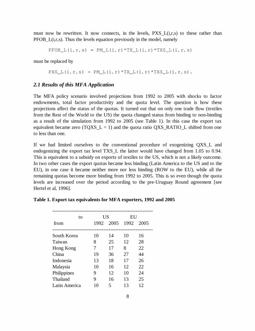
The MFA policy scenario involved projections from 1992 to 2005 with shocks to factorendowments, total factor productivity and the quota level. The question is how theseprojections affect the status of the quotas. It turned out that on only one trade flow (textilesfrom the Rest of the World to the US) the quota changed status from binding to non-bindingas a result of the simulation from 1992 to 2005 (see Table 1). In this case the export taxequivalent became zero (TQXS_L = 1) and the quota ratio QXS_RATIO_L shifted from oneto less than one.

If we had limited ourselves to the conventional procedure of exogenizing QXS_L andendogenizing the export tax level TXS_L the latter would have changed from 1.05 to 0.94.This is equivalent to a subsidy on exports of textiles to the US, which is not a likely outcome.In two other cases the export quotas became less binding (Latin America to the US and to theEU), in one case it became neither more nor less binding (ROW to the EU), while all theremaining quotas become more binding from 1992 to 2005. This is so even though the quotalevels are increased over the period according to the pre-Uruguay Round agreement [seeHertel et al, 1996].

Table 1. Export tax equivalents for MFA exporters, 1992 and 2005

-----------------------------------------------------------to US EU

from 1992 2005 1992 2005 ----------------------------------------------------------- South Korea 10 14 10 16 Taiwan 8 25 12 28 Hong Kong 7 17 8 22 China 19 36 27 44 Indonesia 13 18 17 26 Malaysia 10 16 12 22 Philippines 9 12 10 24 Thailand 9 16 13 25 Latin America 10 5 13 12

9

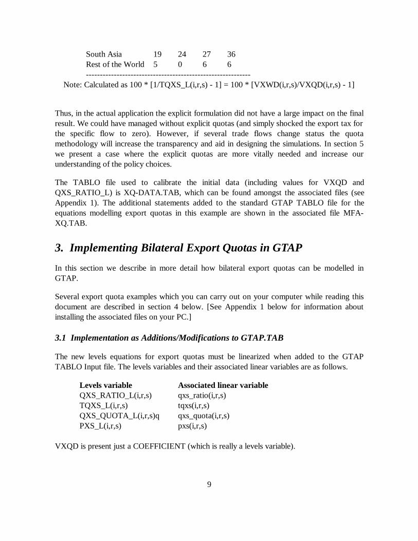
South Asia 19 24 27 36 Rest of the World 5 0 6 6 -----------------------------------------------------------

Note: Calculated as 100 * [1/TQXS_L(i,r,s) - 1] = 100 * [VXWD(i,r,s)/VXQD(i,r,s) - 1]

Thus, in the actual application the explicit formulation did not have a large impact on the finalresult. We could have managed without explicit quotas (and simply shocked the export tax forthe specific flow to zero). However, if several trade flows change status the quotamethodology will increase the transparency and aid in designing the simulations. In section 5we present a case where the explicit quotas are more vitally needed and increase ourunderstanding of the policy choices.

The TABLO file used to calibrate the initial data (including values for VXQD andQXS_RATIO_L) is XQ-DATA.TAB, which can be found amongst the associated files (seeAppendix 1). The additional statements added to the standard GTAP TABLO file for theequations modelling export quotas in this example are shown in the associated file MFA-XQ.TAB.

3. Implementing Bilateral Export Quotas in GTAP

In this section we describe in more detail how bilateral export quotas can be modelled inGTAP.

Several export quota examples which you can carry out on your computer while reading thisdocument are described in section 4 below. [See Appendix 1 below for information aboutinstalling the associated files on your PC.]

3.1 Implementation as Additions/Modifications to GTAP.TAB

The new levels equations for export quotas must be linearized when added to the GTAPTABLO Input file. The levels variables and their associated linear variables are as follows.

Levels variable Associated linear variableQXS_RATIO_L(i,r,s) qxs_ratio(i,r,s)TQXS_L(i,r,s) tqxs(i,r,s)QXS_QUOTA_L(i,r,s)q qxs_quota(i,r,s)PXS_L(i,r,s) pxs(i,r,s)

VXQD is present just a COEFFICIENT (which is really a levels variable).

10

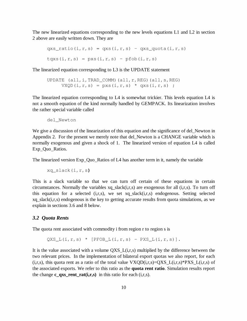
The new linearized equations corresponding to the new levels equations L1 and L2 in section2 above are easily written down. They are

qxs_ratio(i,r,s) = qxs(i,r,s) - qxs_quota(i,r,s)

tqxs(i,r,s) = pxs(i,r,s) - pfob(i,r,s)

The linearized equation corresponding to L3 is the UPDATE statement

UPDATE (all,i,TRAD_COMM)(all,r,REG)(all,s,REG)VXQD(i,r,s) = pxs(i,r,s) * qxs(i,r,s) ;

The linearized equation corresponding to L4 is somewhat trickier. This levels equation L4 isnot a smooth equation of the kind normally handled by GEMPACK. Its linearization involvesthe rather special variable called

del_Newton

We give a discussion of the linearization of this equation and the significance of del_Newton inAppendix 2. For the present we merely note that del_Newton is a CHANGE variable which isnormally exogenous and given a shock of 1. The linearized version of equation L4 is calledExp_Quo_Ratios.

The linearized version Exp_Quo_Ratios of L4 has another term in it, namely the variable

xq_slack(i,r,s )

This is a slack variable so that we can turn off certain of these equations in certaincircumstances. Normally the variables xq_slack(i,r,s) are exogenous for all (i,r,s). To turn offthis equation for a selected (i,r,s), we set xq_slack(i,r,s) endogenous. Setting selectedxq_slack(i,r,s) endogenous is the key to getting accurate results from quota simulations, as weexplain in sections 3.6 and 8 below.

3.2 Quota Rents

The quota rent associated with commodity i from region r to region s is

QXS_L(i,r,s) * [PFOB_L(i,r,s) - PXS_L(i,r,s)].

It is the value associated with a volume QXS_L(i,r,s) multiplied by the difference between thetwo relevant prices. In the implementation of bilateral export quotas we also report, for each(i,r,s), this quota rent as a ratio of the total value VXQD(i,r,s)=QXS_L(i,r,s)*PXS_L(i,r,s) ofthe associated exports. We refer to this ratio as the quota rent ratio. Simulation results reportthe change c_qxs_rent_rat(i,r,s) in this ratio for each (i,r,s).

11

For example, if PFOB_L is 1.2 and PXS_L is 1 then the associated quota rent is QXS_L(1.2 -1.0) and so the associated quota rent ratio is 0.2. If the pre-simulation value of this quota rentratio was zero (meaning that the quota was not binding), then the simulation result for variablec_qxs_rent_rat would be 0.2 (a 0.2 increase from 0.0 to 0.2).

3.3 TABLO Statements for Export Quotas

The equations above for bilateral export quotas need to be added to the standard TABLOInput file for GTAP. Appendix 2 shows the TABLO statements for implementing such exportquotas. Those shown are the ones used in the examples described in section 4 below. [For theMFA example described in section 2 above, slightly different TABLO statements were addedbecause there quotas were only implemented for a subset of the commodities and regions - seethe note near the start of Appendix 2 about this.]

3.4 Assigning Initial QXS_RATIO_L and VXQD Values

For each (i,r,s), we need to set up suitable QXS_RATIO_L(i,r,s) and VXQD(i,r,s) values.Different (i,r,s) triples will probably need different treatments.

If the quota is thought to be not binding,

• VXQD(i,r,s) must be set equal to VXWD(i,r,s);

• the QXS_RATIO_L(i,r,s) value put on the GTAPQUOTA file must not be larger thanone. The QXS_RATIO_L(i,r,s) tells what fraction of the quota you believe the currentexport volume represents so the value assigned will reflect your best information as to howfar the quota is from being binding. If it is nearly binding, you will want a value just lessthan one. If it is a long way from binding you will want a smaller value.

If the quota is thought to be binding,

• QXS_RATIO_L(i,r,s) must be set equal to one;

• the VXQD(i,r,s) value must be no larger than VXWD(i,r,s). The more binding the quota isthought to be, the greater will be the difference between VXWD and VXQD. If you thinkthat the quota is just binding you could set VXQD=VXWD. If you think that the quota isvery restrictive you would set VXQD significantly less than VXWD. In some cases youmight look at the VXMD=PM*QXS values for guidance; if you have VXMD < VXWDand you think that there are no normal export taxes but that all the difference betweenVXMD and VXWD is due to the export quota, you could set VXQD equal to VXMD[This is essentially what was done in the MFA example described in section 2 above.]

12

3.5 Closures for the Model

The normal (or standard) closure for the GTAP model with export quotas has the usual GTAPvariables exogenous. In addition, all components of the linear variables

qxs_quota and xq_slack are exogenous

and the variable

del_Newton is exogenous.

All other new linear variables (namely qxs, pxs, qxs_ratio and tqxs) are endogenous in thisclosure.

To obtain accurate solutions of a simulation with a version of GTAP which includes exportquotas involves solving the model twice. The first calculation is done to see which quotaschange from binding to non-binding or vice versa. In the second calculation we modify theclosure to set qxs_ratio(i,r,s) exogenous and xq_slack(i,r,s) endogenous for those (i,r,s) forwhich the quota has changed from non-binding to binding, and to set tqxs(i,r,s) exogenous andxq_slack(i,r,s) endogenous for those (i,r,s) for which the quota has changed from binding tonon-binding. [See section 3.6 below for more detail.]

3.6 Accurate Export Quota Solutions

To obtain accurate solutions of a model implemented and solved using GEMPACK usuallyinvolves extrapolating after 3 different multi-step calculations (see, for example, section 4 ofHarrison and Pearson (1994)). The theory underpinning extrapolation relies on the underlyinglevels equations being smooth (Pearson,1991). However the Exp_Quo_Ratios equation(equation L4 in section 2 above) is not smooth and so we need a slightly different strategywith a model which has explicit export (or import) quotas. The strategy is as follows.

(a) First do an approximate simulation using a single Euler multi-step calculation (forexample, a 10-step Euler calculation). Here the closure and shocks are those for theapplication you are carrying out, and a shock of one should be given to the variabledel_Newton The sole purpose of this is to find which quotas change their binding/non-binding status (that is, which change from binding to non-binding and which change fromnon-binding to binding). The number of Euler steps must be sufficient to get this correct.[The examples in section 4 below say more about this.] Always use Euler's method forthis simulation, never Gragg's or the midpoint method.

(b) Then do an accurate simulation (extrapolating from 3 multi-step calculations, usingGragg or any other method as appropriate). In this calculation, a closure swap is used toset exogenous qxs_ratio(i,r,s) for all (i,r,s) for which the quota changes in (a) from non-

13

binding to binding and to set exogenous tqxs(i,r,s) for all (i,r,s) for which the quotachanges in (a) from binding to non-binding (in each case, setting the corresponding slackvariable xq_slack(i,r,s) in the Exp_Quo_Ratios equations endogenous). No shock needbe given to the variable del_Newton in this accurate simulation.

The details of this will become much clearer when you carry out some of the examples insection 4 below. We suggest that you at least skim the rest of this section before doing theseexamples. We also suggest that you re-read this section carefully after carrying out theexamples: the details here will probably seem much more straightforward after you have donea few of the examples.

Exact shocks for the components of qxs_ratio and tqxs set exogenous in the accuratecalculation in (b) can be calculated from a knowledge of the pre-simulationQXS_RATIO_L(i,r,s) and TQXS_L(i,r,s) levels values. Indeed,

• if the quota on exports of commodity i from region r to region s changes from non-binding to binding, you know that the post-simulation value of QXS_RATIO_L(i,r,s) mustbe one (this is exactly what binding means). The pre-simulation value ofQXS_RATIO_L(i,r,s) is on the GTAPQUOTA data file. Hence it is easy to work out thepercentage change in QXS_RATIO_L(i,r,s): this is the shock to give qxs_ratio(i,r,s) in theaccurate simulation.

• if the quota on exports of commodity i from region r to region s changes from bindingto non-binding, you know that the post-simulation value of the price ratio TQXS_L(i,r,s)must be 1 (since the post-simulation value of QXS_RATIO_L(i,r,s) is less than one andequation Exp_Quo_Ratios must hold). The pre-simulation value of TQXS_L(i,r,s) can beobtained from the Display file produced by calculation (a) and so it is easy to work out thepercentage change in TQXS_L(i,r,s): this is the shock to give to tqxs(i,r,s) in the accuratesimulation.

A TABLO Input file XQ-BIND.TAB supplied with the associated files calculates theqxs_ratio and tqxs shocks required for the accurate simulation.

The closure used in the accurate simulation is that from (a) with the swaps indicated above.We discuss automating the setting up of this closure in section 8.3 below.

3.6.1 Checking the Accurate Simulation

It is important to check that the accurate simulation (the one in (b) above) has workedcorrectly. As well as checking the convergence, you should check that the same quotas arebinding in the post-simulation data from the accurate simulation as were binding after theapproximate simulation. You must also check that the post-simulation values of the quantityand price ratios QXS_RATIO_L and TQXS_L are as expected [that is, not larger than one

14

and having maximum one for each relevant (i,r,s)]. The file TABLO Input file XQCHK.TAB(see the examples in section 4 below) can be used to check this. This checking ofQXS_RATIO_L and TQXS_L values is necessary to ensure that the initial (approximate)simulation was sufficiently accurate to correctly identify the quotas which change theirbinding/non-binding nature.

If this check fails, it indicates that the approximate simulation in (a) did not have enough Eulersteps. Thus the remedy is to redo the approximate calculation with more Euler steps and thenredo the accurate simulation and check it again.

4. Export Quotas in a 3x3 Version of GTAP

This section introduces the export quota examples associated with this document. Detailedinstructions for carrying out these are also given in the file XQ.TXT .

The relevant TABLO Input file is GTAP33XQ.TAB which can be found in the associatedexamples in the file QUOTA-EX.ZIP (see Appendix 1 below to see how to install theseexamples on your PC). This file is based on the standard TABLO Input file GTAP94.TAB forGTAP. The maximum set sizes have been reduced so that at most 3 tradeable commoditiesand 3 regions are allowed. An additional section containing the TABLO implementation of theexport quota equations is added at the end. The original EXPRICES equation is modified asindicated in section 3 above. The export quota part of this file GTAP33XQ.TAB is shown infull in Appendix 2.

As indicated above in sections 2 and 3.4, supplementary data are required for these quotas.We have added the VXQD data, which are set equal to the usual VXWD data, at header"VXQD". The resulting GTAPDATA file is the file DAT201XQ.HAR which is identical tothe standard 3-tradeable-commodity, 3-region file DAT2-01.HAR with the VXQD dataadded. By setting VXQD=VXWD we are assuming that none of the export quotas arebinding in the initial data.

The other supplementary data needed are the QXS_RATIO_L(i,r,s) values. These are heldon the text file XQ2-01.DAT which is the actual file corresponding to the logical file calledGTAPQUOTA in GTAP33XQ.TAB. Since no quotas are binding, all QXS_RATIO_L valueson this file are less than 1. We have set these ratios

• equal to 0.98 for exports of manufactures "mnfcs" from the Rest of the World "ROW" toboth the United States "USA" and the European Union "EU". This value means thatthese two quotas are nearly binding.

• equal to 0.2 in all other cases, which means that these other quotas are far from binding.

15

The first examples A1-A7 are ones in which the only shocks to the model are to change thelevel of various quotas. Detailed instructions for carrying out these examples are given in thefile XQ.TXT . The second examples P1 and P2 are more realistic in that there the exportquotas are not shocked - rather the example looks at the effect of the existing quotas on aprojection simulation (a stylized version of that described in section 2 above) aimed at takingthe economy from 1992 to 2005.

We encourage you to install the relevant files on your PC (following the instructions inAppendix 1 below) and then to carry out these examples before reading further in this paper.This should give you a clear understanding of what is involved in solving GTAP with explicitexport quotas. [If you don’t have a version of GEMPACK on your PC, you can obtain theDemonstration Version of GEMPACK at no cost from the World-Wide Web - see Appendix 1for details - and use this to carry out the export quota examples.]

5. Bilateral Import Quotas

The need for bilateral import quotas grew out from research on China and grain imports.Chinese agricultural policies are at an important turning point these years as production ofagricultural commodities fails to keep pace with consumption. The pressure for agriculturalprotection and support is increasing. The second Chinese offer to the World TradeOrganization (WTO) within the ongoing negotiations for Chinese membership displays thisconcern. The offer contains tariff quotas on wheat and coarse grains with above-quota tarifflevels being so high that they will effectively block imports [WTO, 1994].

For wheat the proposed tariff quota will fix imports at 9.76 million tons and for barley at0.785 million tons between 1995 and 2004. Compared with the base period quantity ofimports it is evident that this will essentially fix import quantities at the 1992 level. In thequota scenario it is therefore assumed that the quota equals the 1992 import level and remainsunchanged to the year 2005. We extend this assumption to rice as well (for rice the base yearimport quantities are very low but if high import quantities should appear, a logicalconsequence would be an import quota on rice as well).

Once again these quotas could have been modelled by simply fixing the quantity flows(QXS_L) and endogenizing the tariff rate (TMS_L). In this case, however, the approach isinadequate, as we simultaneously need to cut the tariff on coarse grains. Moreover, we are stillstuck with the problem, that if we simply use the bilateral trade flow and endogenize the tariff,the quota could change status from binding to non-binding with potentially misleading results.

Finally, it is attractive from a policy perspective to trace the specific tariff equivalents of thequotas.

16

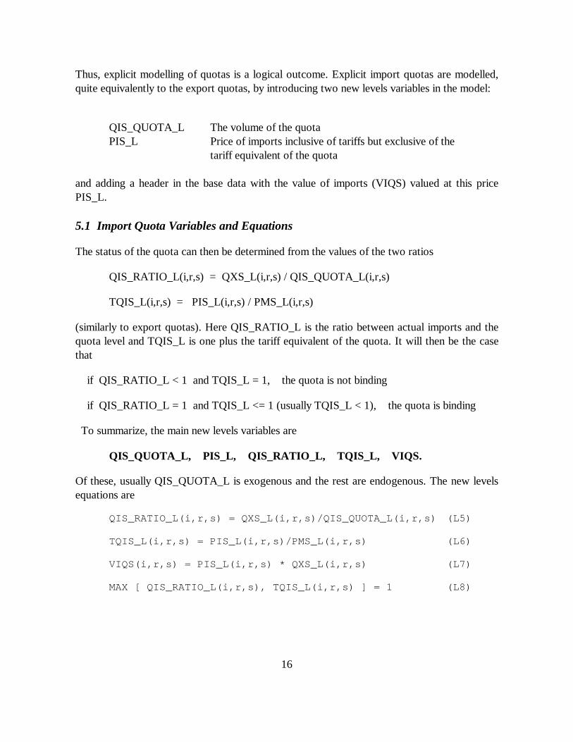
Thus, explicit modelling of quotas is a logical outcome. Explicit import quotas are modelled,quite equivalently to the export quotas, by introducing two new levels variables in the model:

QIS_QUOTA_L The volume of the quotaPIS_L Price of imports inclusive of tariffs but exclusive of the

tariff equivalent of the quota

and adding a header in the base data with the value of imports (VIQS) valued at this pricePIS_L.

5.1 Import Quota Variables and Equations

The status of the quota can then be determined from the values of the two ratios

QIS_RATIO_L(i,r,s) = QXS_L(i,r,s) / QIS_QUOTA_L(i,r,s)

TQIS_L(i,r,s) = PIS_L(i,r,s) / PMS_L(i,r,s)

(similarly to export quotas). Here QIS_RATIO_L is the ratio between actual imports and thequota level and TQIS_L is one plus the tariff equivalent of the quota. It will then be the casethat

if QIS_RATIO_L < 1 and TQIS_L = 1, the quota is not binding

if QIS_RATIO_L = 1 and TQIS_L <= 1 (usually TQIS_L < 1), the quota is binding

To summarize, the main new levels variables are

QIS_QUOTA_L, PIS_L, QIS_RATIO_L, TQIS_L, VIQS.

Of these, usually QIS_QUOTA_L is exogenous and the rest are endogenous. The new levelsequations are

QIS_RATIO_L(i,r,s) = QXS_L(i,r,s)/QIS_QUOTA_L(i,r,s) (L5)

TQIS_L(i,r,s) = PIS_L(i,r,s)/PMS_L(i,r,s) (L6)

VIQS(i,r,s) = PIS_L(i,r,s) * QXS_L(i,r,s) (L7)

MAX [ QIS_RATIO_L(i,r,s), TQIS_L(i,r,s) ] = 1 (L8)

17

Once again, there are 5 lots of new levels variables and 4 lots of new levels equations. This isconsistent with just one lot of these (usually the QIS_QUOTA_L values) being setexogenously. The model should then determine the rest of these.

In addition to the above new equations, the equation MKTPRICES connecting the cif price ofimports pcif(i,r,s) to the domestic price pms(i,r,s) and "normal" import tariffs tm(i,r) andtms(i,r,s) must now be rewritten. It now connects, in the levels, PIS_L(i,r,s) to these ratherthan PMS_L(i,r,s). Thus the levels equation previously in the model, namely

PMS_L(i,r,s) = PCIF_L(i,r,s)*TM_L(i,r)*TMS_L(i,r,s)

must be replaced by

PIS_L(i,r,s) = PCIF_L(i,r,s)*TM_L(i,r)*TMS_L(i,r,s)

5.2 Calibrating VIQS and QIS_RATIO_L Values for this Application

In this application we have a situation where the base data does not contain any quotas orquota tax equivalents. The policy scenario is to implement quotas from a quota free (but lowimport) situation in 1992. Thus, all quotas are equal to the exact imports but no tariffequivalents have yet developed. The new header with the quota information is simply addedwith the statement

VIQS(i,r,s) = VIMS(i,r,s)

Essentially, we wish to calibrate the model so that all quotas are just binding in the base data(QIS_RATIO_L = 1). However, it turns out that if we do this in those cases where the initialtrade volume is zero (and remains zero) the matrix becomes singular during a simulation. Inthose cases we must assume that the quota is not-binding and we end up having a mix ofbinding and non-binding quotas given by:

QIS_RATIO_L(i,r,s) = 1 if VIMS(i,r,s) is larger than zero,

QIS_RATIO_L(i,r,s) = 0.9 if VIMS(i,r,s) is zero.

Once again the value 0.9 is arbitrarily chosen. But in this case it makes no difference as themodel code assures that trade flows that are initially zero remains zero.

5.3 Results of this Application

Once again the simulations involve projections from the year 1992 to 2005. Three differentscenarios are presented. The first is a baseline with shocks to factor endowments, total factorproductivity and implementation of the trade reforms agreed upon in the GATT UruguayRound. The second scenario is the baseline plus liberalization in China according to the second

18

schedule submitted to the WTO, but without the quotas. The third scenario adds the importquotas on grain.

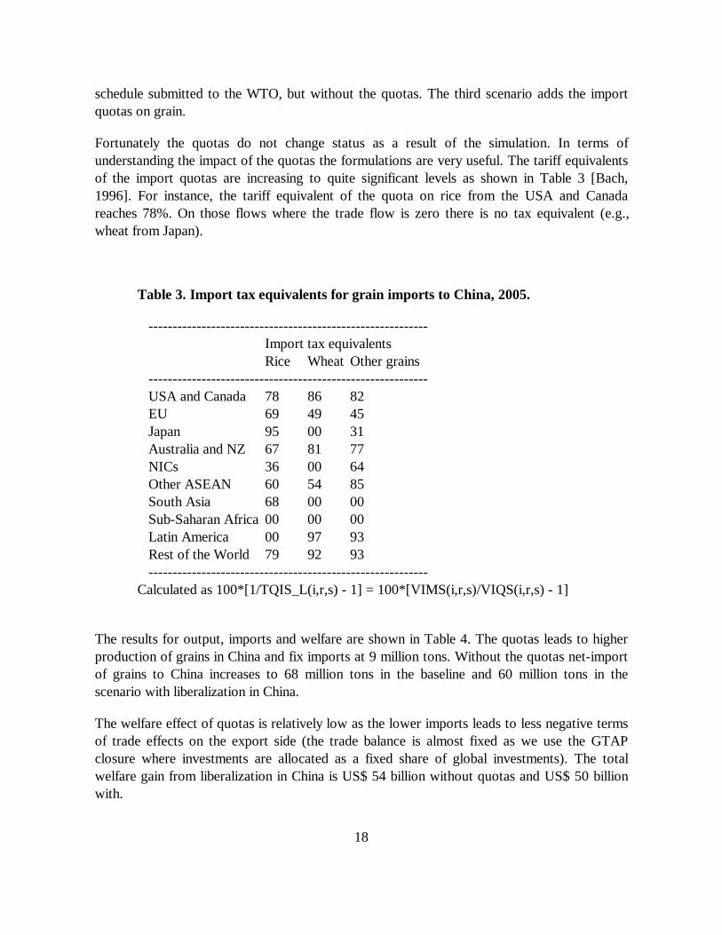
Fortunately the quotas do not change status as a result of the simulation. In terms ofunderstanding the impact of the quotas the formulations are very useful. The tariff equivalentsof the import quotas are increasing to quite significant levels as shown in Table 3 [Bach,1996]. For instance, the tariff equivalent of the quota on rice from the USA and Canadareaches 78%. On those flows where the trade flow is zero there is no tax equivalent (e.g.,wheat from Japan).

Table 3. Import tax equivalents for grain imports to China, 2005.

----------------------------------------------------------Import tax equivalentsRice Wheat Other grains

---------------------------------------------------------- USA and Canada 78 86 82 EU 69 49 45 Japan 95 00 31 Australia and NZ 67 81 77 NICs 36 00 64 Other ASEAN 60 54 85 South Asia 68 00 00 Sub-Saharan Africa 00 00 00 Latin America 00 97 93 Rest of the World 79 92 93 ----------------------------------------------------------Calculated as 100*[1/TQIS_L(i,r,s) - 1] = 100*[VIMS(i,r,s)/VIQS(i,r,s) - 1]

The results for output, imports and welfare are shown in Table 4. The quotas leads to higherproduction of grains in China and fix imports at 9 million tons. Without the quotas net-importof grains to China increases to 68 million tons in the baseline and 60 million tons in thescenario with liberalization in China.

The welfare effect of quotas is relatively low as the lower imports leads to less negative termsof trade effects on the export side (the trade balance is almost fixed as we use the GTAPclosure where investments are allocated as a fixed share of global investments). The totalwelfare gain from liberalization in China is US$ 54 billion without quotas and US$ 50 billionwith.

19

Table 4. Output, import and welfare effects in China, 1992-2005.

-----------------------------------------------------------------------------Grain Net-import Welfareproduction of grains effectmn tons mn tons bn US$

------------------------------------------------------------------------------BASELINE 535 68 -China lib. schedule 514 60 54China lib.+ quotas 578 9 50------------------------------------------------------------------------------

In this case the quota formulation gives us additional insights and allows us to introducequotas while simultaneously changing the import tariffs.

The TABLO file used to calibrate the initial data for this application (including values for thearrays VIQS and QIS_RATIO_L) is IQ-DATA.TAB, which can be found amongst theassociated files (see Appendix 1). The additional statements added to the standard GTAPTABLO file for the equations modelling import quotas in this example are shown in theassociated file CHINA-IQ.TAB.

6. Bilateral Import Quotas in GTAP

In this section we describe how import quotas can be modelled in GTAP. As this is quitesimilar to section 3 for export quotas, the discussion is more brief.

6.1 Implementation as Additions/Modifications to GTAP.TAB

The new levels equations must be linearized when added to the GTAP TABLO Input file. Thelevels variables and their associated linear variables are as follows.

Levels variable Associated linear variableQIS_RATIO_L(i,r,s) qis_ratio(i,r,s)TQIS_L(i,r,s) tqis(i,r,s)QIS_QUOTA_L(i,r,s)q qis_quota(i,r,s)PIS_L(i,r,s) pis(i,r,s)

VIQS is present just a COEFFICIENT (which is really a levels variable).

20

The new linearized equations corresponding to the new levels equations L5 and L6 are easilywritten down. They are

qis_ratio(i,r,s) = qxs(i,r,s) - qis_quota(i,r,s)

tqis(i,r,s) = pis(i,r,s) - pms(i,r,s)

The linearized equation corresponding to L7 is the UPDATE statement

UPDATE (all,i,TRAD_COMM)(all,r,REG)(all,s,REG)VIQS(i,r,s) = pis(i,r,s) * qxs(i,r,s) ;

Once again it is the MAX equation corresponding to L8 which causes problems. Thelinearization of this Imp_Quo_Ratios equation is quite similar to the export quota casedescribed in Appendix 3, so we will only give the result:

IF[ QIS_RATIO_L(i,r,s) >= TQIS_L(i,r,s), QIS_RATIO_L(i,r,s)/100*qis_ratio(i,r,s) ] + IF[ QIS_RATIO_L(i,r,s) < TQIS_L(i,r,s), TQIS_L(i,r,s)/100*tqis(i,r,s) ] + [ MAX {QIS_RATIO_L(i,r,s), TQIS_L(i,r,s)} - 1 ] * del_Newton + iq_slack(i,r,s) = 0 ;

As in the export quota case, the equation contains the variable del_Newton to make sure thatthe two ratios QIS_RATIO_L and TQIS_L do not get larger than 1, and the slack variableiq_slack which allows us to turn off the equation for those flows where we do not need it.

6.2 Quota rents

The quota rents associated with the import quotas on commodity i from region r to region sare in this case the difference between the value of imports outside the border and the valueinside the country after the quota constraint but before the “normal” import tariffs.Specifically, we are interested in the quota rent as a ratio of the total value of imports inclusivethe “normal” import tariffs:

QIS_RENT_RATIO_L = [QXS_L*(PMS_L-PIS_L)]/[QXS_L*PIS_L] = [PMS_L/PIS_L] - 1 = [1/TQIS] - 1

Linearized this equation becomes:

c_qis_rent_rat(i,r,s) = -{1/[100*TQIS_L(i,r,s)]} *tqis(i,r,s)

21

where c_qis_rent_rat is the change in the quota rate ratio (a change variable).

6.3 TABLO Statements for Import Quotas

The entire block of declarations, coefficients and equations for modelling import quotas can befound in the file GTAP33IQ.TAB. Again these quotas are written to make it possible tointroduce quotas on all bilateral flows in the model. In the application described in section 5,import quotas were only introduced on grain imports to China with the use of appropriateSET definitions. This reduces the amount of variables and the size of the model, which can beconvenient or even necessary in some cases.

6.4 Assigning Initial QIS_RATIO_L and VIQS Values

For each (i,r,s), we need to set up suitable QIS_RATIO_L(i,r,s) and VIQS(i,r,s) values.Different (i,r,s) triples will probably need different treatments.

If the import quota is thought to be not binding,

• VIQS(i,r,s) must be set equal to VIMS(i,r,s);

• the QIS_RATIO_L(i,r,s) value put on the GTAPQUOTA file must not be larger than one.The QIS_RATIO_L(i,r,s) tells what fraction of the quota you believe the current importvolume represents so the value assigned will reflect your best information as to how far thequota is from being binding. If it is nearly binding, you will want a value just less than one.If it is a long way from binding you will want a smaller value.

If the quota is thought to be binding,

• QIS_RATIO_L(i,r,s) must be set equal to one;

• the VIQS(i,r,s) value must be no larger than VIMS(i,r,s). The more binding the quota isthought to be, the greater will be the difference between VIMS and VIQS. If you thinkthat the quota is just binding you could set VIQS=VIMS. If you think that the quota isvery restrictive you would set VIQS significantly less than VIMS. In some cases youmight look at the VIWS=PCIF*QXS values for guidance; if you have VIWS < VIMS andyou think that there are no normal import tariffs but that all the difference between VIWSand VIMS is due to the import quota, you could set VIQS equal to VIMS.

6.5 Closures for the Model

Beyond the normal (or standard) closure of the GTAP model the following variables must beadded to the list of exogenous variables in the Command file:

22

qis_quota

iq_slack

del_Newton

All other new linear variables (qis, pis, pis_ratio and tqis) are endogenous. If you wish to run asimulation without any quota constraints just endogenize iq_slack and exogenize tqis. This is aconvenient way to test that the model still behaves exactly as the standard GTAP modelwithout quotas.

When solving the model accurately after the first approximate run, qis_ratio(i,r,s) must beswapped with iq_slack(i,r,s) for those bilateral flows where the quota changes status fromnon-binding to binding and tqis(i,r,s) must be swapped with iq_slack(i,r,s) for those flowswhere the quota changes status from binding to non-binding. [See section 6.6 below for moredetails.]

6.6 Accurate Import Quota Solutions

As with export quotas, this involves first doing an approximate (Euler) simulation to findwhich quotas change their binding/non-binding status, and then doing an accurate simulationusing this knowledge. In the accurate simulation, a closure swap is used to set exogenousqis_ratio(i,r,s) for all (i,r,s) for which the quota changes from non-binding to binding and toset exogenous tqis(i,r,s) for all (i,r,s) for which the quota changes from binding to non-binding(in each case, setting the corresponding slack variable iq_slack(i,r,s) in the Imp_Quo_Ratiosequations endogenous). A shock of one is given to variable del_Newton in the approximatesimulation but no shock needs to be given to this variable in the accurate simulation.

Exact shocks for the components of qis_ratio and tqis set exogenous in the accuratesimulation can be calculated from a knowledge of the pre-simulation QIS_RATIO_L(i,r,s) andTQIS_L(i,r,s) levels values. Indeed,

• if the quota on imports of commodity i from region r to region s changes from non-binding to binding, you know that the post-simulation value of QIS_RATIO_L(i,r,s) mustbe one (this is exactly what binding means). The pre-simulation value ofQIS_RATIO_L(i,r,s) is on the GTAPQUOTA data file. Hence it is easy to work out thepercentage change in QIS_RATIO_L(i,r,s): this is the shock to give qis_ratio(i,r,s) in theaccurate simulation.

• if the quota on imports of commodity i from region r to region s changes from bindingto non-binding, you know that the post-simulation value of the price ratio TQIS_L(i,r,s)must be 1 (since the post-simulation value of QIS_RATIO_L(i,r,s) is less than one andequation Imp_Quo_Ratios must hold). The pre-simulation value of TQIS_L(i,r,s) can be

23

obtained from the Display file produced during the approximate simulation and so it is easyto work out the percentage change in TQIS_L(i,r,s): this is the shock to give to tqis(i,r,s) inthe accurate simulation.

A TABLO Input file IQ-BIND.TAB supplied with the associated files calculates the qis_ratioand tqis shocks required for the accurate simulation.

The closure used in the accurate simulation is that from the approximate simulation with theswaps indicated above. We discuss automating the setting up of this closure in section 8.3below.

6.6.1 Checking the Accurate Simulation

As with export quotas, it is important to check that the accurate simulation has workedcorrectly. As well as checking the convergence, you should check that the same quotas arebinding in the post-simulation data from the accurate simulation as were binding after theapproximate simulation. You must also check that the post-simulation values of the quantityand price ratios QIS_RATIO_L and TQIS_L are as expected [that is, not larger than one andhaving maximum one for each relevant (i,r,s)]. The file TABLO Input file IQCHK.TAB (seethe examples in section 7 below) can be used to check this. This checking of QIS_RATIO_Land TQIS_L values is necessary to ensure that the initial (approximate) simulation wassufficiently accurate to correctly identify the quotas which change their binding/non-bindingnature.

If this check fails, it indicates that the approximate simulation did not have enough Euler steps.Thus the remedy is to redo the approximate calculation with more Euler steps and then redothe accurate simulation and check it again.

7. Import Quotas in a 3x3 Version of GTAP

We now turn to the associated import quota examples, which involve a 3x3 version of theGTAP model and database. Detailed instructions are contained in the file IQ.TXT .

The relevant TABLO Input file is GTAP33IQ.TAB, which can be found in the associatedexamples in the file QUOTA-EX.ZIP (see Appendix 1). The quota section is found at the veryend of the file. When starting with a standard GTAP database we first need to,

1) add the header VIQS.

2) create a file with the values of QIS_RATIO_L.

As in section 5 we assume that initially all quotas are just binding but that no quota rents arepresent. That is QIS_RATIO_L and TQIS_L are both equal to one and the new VIQS data

24

are set equal to the VIMS values. In the standard 3x3 GTAP data, there are no zeros in theVIMS data since very small values are shown even for imports from both USA and EU tothemselves.

These two steps are conveniently done with the TABLO file IQ-DATA.TAB (see the fileIQ.TXT for details).

Again we encourage you to work through the associated import quota examples on your PCbefore you read further in this document. There are three examples called B1, B2 and B3.They all involve shocks to import tariffs with import quotas on food in place.

A noteworthy feature of these import quota examples is that the quota constraints are limitedto the commodity FOOD: this is done by endogenizing the variable iq_slack for the othercommodities (MNFCS and SVCES) and exogenizing tqis for these commodities. This meansthat, when checking the post-simulation values of QIS_RATIO_L(i,r,s) and TQIS_L(i,r,s)after a hopefully accurate import quota simulation, only the values for i=FOOD need to bechecked.

8. Automating the Second Part of the Two-Part SolutionProcedure

In this section we set out the procedure for the bilateral export quota case. The procedure forbilateral import quotas is very similar - we leave the details to our readers.

The second more accurate simulation in the bilateral export quota case may require a closurechange from the first (approximate) simulation and may require shocks to be given to somecomponents of variables qxs_quota and tqxs. The procedure to use with Release 5.1 (April1994) of GEMPACK is set out in sections 8.1 and 8.2 below. A simpler procedure that onlyworks with Release 5.2 (September 1996) of GEMPACK is set out in section 8.3 below.

8.1 Automating the Shocks

Automating calculation of the shocks is straightforward and uses the familiar technique ofcalculating all possible values via a data-manipulation TABLO Input file and selecting thoserequired via statements of the form

shock qxs_ratio("mnfcs","ROW","USA") = select from file <FILE1> ;shock tqxs("mnfcs","ROW","EU") = select from file <FILE2> ;

on your Command file. [This technique is similar to the GTAP method of calculating shocks toremove distortions via SHOCKS.TAB.]

25

The TABLO Input file to calculate shocks for bilateral export quotas is called XQ-BIND.TAB . [This is one of the files associated with this document.] If you examine it, youwill see that it relies on reading both the pre-simulation data (GTAPDATA andGTAPQUOTA files) and also the post-simulation data files produced by the first approximateversion of the simulation. It looks at both to first identify which quotas have changed theirbinding/non-binding status and then writes two text files intended to be used as shocks files forthe variables qxs_ratio and tqxs respectively. In each case, nonzero values are only written forthose components for which the binding/non-binding status changes. [The qxs_ratio shocksfile only has a nonzero value for (i,r,s) when the export quota for this changes from non-binding to binding. The tqxs shocks file only has a nonzero value for (i,r,s) when the exportquota for this changes from binding to non-binding.]

Carrying out the calculation of these two shocks files is straightforward. All you need is aCommand file with the appropriate files associated with each logical file. The file BIND-A1.CMF shows how to do this. In the shocks statements above, FILE1 is the name of theactual file with logical name QXS_RAT_SH produced from XQ-BIND.TAB and FILE2 is thename of the actual file with logical name TQXS_SH produced from XQ-BIND.TAB.

Using these shocks files in the accurate simulation is also quite straightforward. You merelyneed to insert one shock statement (same format as the example above) for each relevantcomponent. Specifically, you need one such qxs_ratio shock statement for each (i,r,s) forwhich the quota changes from non-binding to binding, and you need one such tqxs shockstatement for each (i,r,s) for which the quota changes from binding to non-binding. [See, forexample, the Command file XQ-A6.CMF used in Example A6.]

The need to do this separately for the different components is removed with Release 5.2 ofGEMPACK, as explained in section 8.3 below.

Note that amongst the associated files is a file IQ-BIND.TAB which does for import quotaswhat XQ-BIND.TAB does for export quotas.

8.2 Automating the Closure Change

The closure changes required are swap statements of the form

swap qxs_ratio("mnfcs","ROW","USA") = xq_slack ("mnfcs","ROW","USA") ;

One such statement is needed for each (i,r,s) for which the quota changes from non-binding tobinding. And one similar statement swapping tqxs with xq_slack is required for eachcomponent which changes from binding to non-binding.

26

With Release 5.1 of GEMPACK, you will need to insert these statements by hand. The shocksfiles produced by running XQ-BIND tell you which components are relevant in each case(since these only contain nonzero values when such a closure swap is indicated).

8.3 Automating Shocks and Closure Swaps with Release 5.2 of GEMPACK

Release 5.2 of GEMPACK has new statements allowed in Command files which make it veryeasy to specify the closure swaps and shocks required for the second accurate calculation.

For the closure change, the following statements

exogenous qxs_ratio = nonzero value on file <FILE1> ;endogenous xq_slack = nonzero value on file <FILE1> ;exogenous tqxs = nonzero value on file <FILE2> ;endogenous xq_slack = nonzero value on file <FILE2> ;

are all that is required in every case. Here FILE1 is the name of the actual file with logicalname QXS_RAT_SH produced from XQ-BIND.TAB and FILE2 is the name of the actualfile with logical name TQXS_SH produced from XQ-BIND.TAB (see section 8.1 above).The first of the statements above is an instruction to set exogenous those components ofvariable qxs_ratio for which the associated value on FILE1 is nonzero; similarly for the otherstatements.

The required shocks to qxs_ratio and tqxs can be specified by the two statements

shock qxs_ratio = select from file <FILE1> ;shock tqxs = select from file <FILE2> ;

where FILE1 and FILE2 are as above.2 [The only time when these statements need to bealtered is when no components of qxs_ratio or tqxs are exogenous; then the shock statementfor this variable must be omitted or commented out.] Note that the same files FILE1 andFILE2 serve to specify the closure changes and the extra shocks.

Thus the second accurate simulation is very easy to set up and run under Release 5.2 ofGEMPACK. After the first approximate version is run, you need to compute the shocks filesby running XQ-BIND (from XQ-BIND.TAB) and to modify the Command file by putting inthe statements above (and making the other changes to the Command file as described earlier).

2The astute reader will notice that these statements should work with Release 5.1 of GEMPACK. However abug in that version of the software means that they will almost certainly not work. This is why werecommended individual shock statements for each relevant (i,r,s) in section 8.1 above.

27

You can then run the simulation required to produce accurate results in the presence of thequotas.

The files XQ-A22.CMF and XQ-A62.CMF in the accompanying files are examples using thisautomation.

8.4 An Alternative Closure for the Accurate Simulation

In some cases it may be better to use an alternative closure for the second accurate simulation.In this alternative closure,

• xq_slack is set endogenous for all (i,r,s) - this turns off equation Exp_Quo_Ratios in allcases,

• qxs_ratio is set exogenous for all (i,r,s) for which you believe the quota will be binding (asindicated by the first approximate simulation),

• tqxs is set exogenous for all other (i,r,s) (that is, for which you believe that the quota willnot be binding).

There may be some simulations in which a quota changes status during the simulation (forexample, changes from binding to non-binding during step 6 of a 10-step calculation) and thenchanges back to its original status by the end. In such a case the results are likely to convergebetter if the associated non-smooth Exp_Quo_Ratios plays no role.

9. Handling Other Inequalities using GEMPACK

We mention very briefly some other inequalities which can arise in CGE models and ways inwhich they can be handled with GEMPACK.

Kuhn-Tucker Conditions

Inequalities often enter GE models in the form of Kuhn-Tucker conditions attached with aninequality or sign constraint. Consider, for example, the Kuhn-Tucker conditions

P - MC <= 0, X >= 0, (P-MC)X=0.

These can be rewritten as

MIN ( X, MC-P ) = 0

(which is equivalent to the three Kuhn-Tucker conditions). This levels equation can thenbe linearized and treated as in the quota cases dealt with above.

28

Non-negative Investment

Investment in each sector of a GE model must be non-negative in each period. MichaelMalakellis has used Mark Horridge's method (essentially as set out in this document - see alsoHorridge, 1993) in his intertemporal model ORANI-INT of the Australian economy to ensurethat investment does indeed stay non-negative for each sector in each period. See Malakellis(1994) for details.

Other Quotas

Other treatments of quotas are easy to imagine. For example, instead of bilateral importquotas by commodity and source, each region may impose a quota on the total imports ofeach commodity (from all other regions). This could be modelled explicitly following similarmethods to those described in this paper.

10. Conclusion

The purpose of this technical paper has been to demonstrate that bilateral export and importquotas (and other inequalities) can be modelled explicitly in GTAP and GEMPACK. If youneed to do so, we hope that this paper and the associated computer files will provide sufficientdetail for you to be able to model these in your application.

The examples in sections 2 and 5 above also make the point that when quotas are relevant toyour application, modelling them explicitly is not necessarily the most appropriate way toproceed.

Modelling such inequalities explicitly using GEMPACK is relatively new. We expect thatmodifications to some of the procedures described here will be suggested as they are usedmore.

29

References

Bach, C.F. (1996), Trade Policies and Food Security in China. Department of Economics andNatural Resources, The Royal Danish Agricultural University, Copenhagen.

Brooke, Anthony, David Kendrick and Alexander Meeraus (1988), GAMS: A User's Guide,The Scientific Press, Redwood City.

Harrison, W.J. and K.R. Pearson (1994), Computing Solutions for Large General EquilibriumModels Using GEMPACK. Monash University, Australia, Impact Project. PreliminaryWorking Paper No. IP-64. [A revised version is in Computational Economics vol. 9(1996), pp.83-127.]

Hertel, T.W. (Ed.) (1996, forthcoming), Global Trade Analysis: Modeling and Applications.Cambridge University Press.

Hertel, T., Bach, C.F., Dimaranan, B., & Martin, W. (1995), Growth, Globalization, andGains from the Uruguay Round. Presented at the Sixth International CGE ModelingConference, October 27, 1995. Waterloo, Ontario.

Horridge, J.M. (1993), Inequality Constraints, unpublished manuscript presented to theGEMPACK Users Day in June 1993.

Malakellis, Michael (1994), ORANI-INT: An Intertemporal GE Model of the AustralianEconomy, PhD Thesis, Monash University.

Pearson, K.R. (1991), Solving Nonlinear Economic Models Accurately via a LinearRepresentation, Impact Preliminary Working Paper No. IP-55, Melbourne (July),pp.39.

Rutherford, Thomas F. (1995), Applied General Equilibrium Modeling with MPSGE as aGAMS Subsystem: An Overview of the Modeling Framework and Syntax, Departmentof Economics, University of Western Ontario.

WTO (1994), People's Republic of China - Draft Final Schedule. Geneva, The World TradeOrganization. Spec(88)13/Add.18.

30

Appendix 1: Installing and Using the Associated Files

The associated files are in the PKZIP file QUOTA-EX.ZIP. This contains TABLO, data andCommand files required for the examples described in this paper. To use them you need an80386/80486/pentium PC running DOS, Microsoft Windows or Windows 95 which has eithera DOS-Lahey source-code version, or the Executable-image version, or the DemonstrationVersion of Release 5.1 or later of GEMPACK installed. If you don’t have any of these, youcan obtain the Demonstration Version at no cost from the GEMPACK World-Wide Web site(the address of which is given later in this section).

[If you have a source-code version of GEMPACK for an operating system other thanDOS/Windows, you could easily convert the files in QUOTA-EX.ZIP for use withGEMPACK on your machine.]

To install the files we suggest that you make a new directory or subdirectory (perhapsC:\QUOTAS) and copy the file QUOTA-EX.ZIP into this directory. You will also need thefile PKUNZIP.EXE in order to unzip the files in QUOTA-EX.ZIP. [The files QUOTA-EX.ZIP and PKUNZIP.EXE can be obtained from the World-Wide Web at the address shownbelow.] Then unzip the files by first changing into this directory and then issuing thecommand

pkunzip quota-ex

You should then be able to carry out the examples described in sections 4 and 7 above byworking in this directory. The files XQ.TXT and IQ.TXT contain detailed instructions forcarrying out export quota examples (section 4) and import quota examples (section 7)respectively.

Obtaining QUOTA-EX.ZIP and/or the Demonstration Version of GEMPACK

These will normally be available from the World-Wide Web on the

• GEMPACK Web site http://www.monash.edu.au/policy/gempack.htm and/or

• the GTAP Web site http://www.agecon.purdue.edu/gtap/

In order to use the Demonstration Version of GEMPACK for the quota examples, you willneed two more .ZIP files besides QUOTA-EX.ZIP, namely XQ-TG.ZIP and IQ-TG.ZIP.These are also normally available from the addresses above.

31

Appendix 2: Additions to GTAP94.TAB

for Bilateral Export Quotas

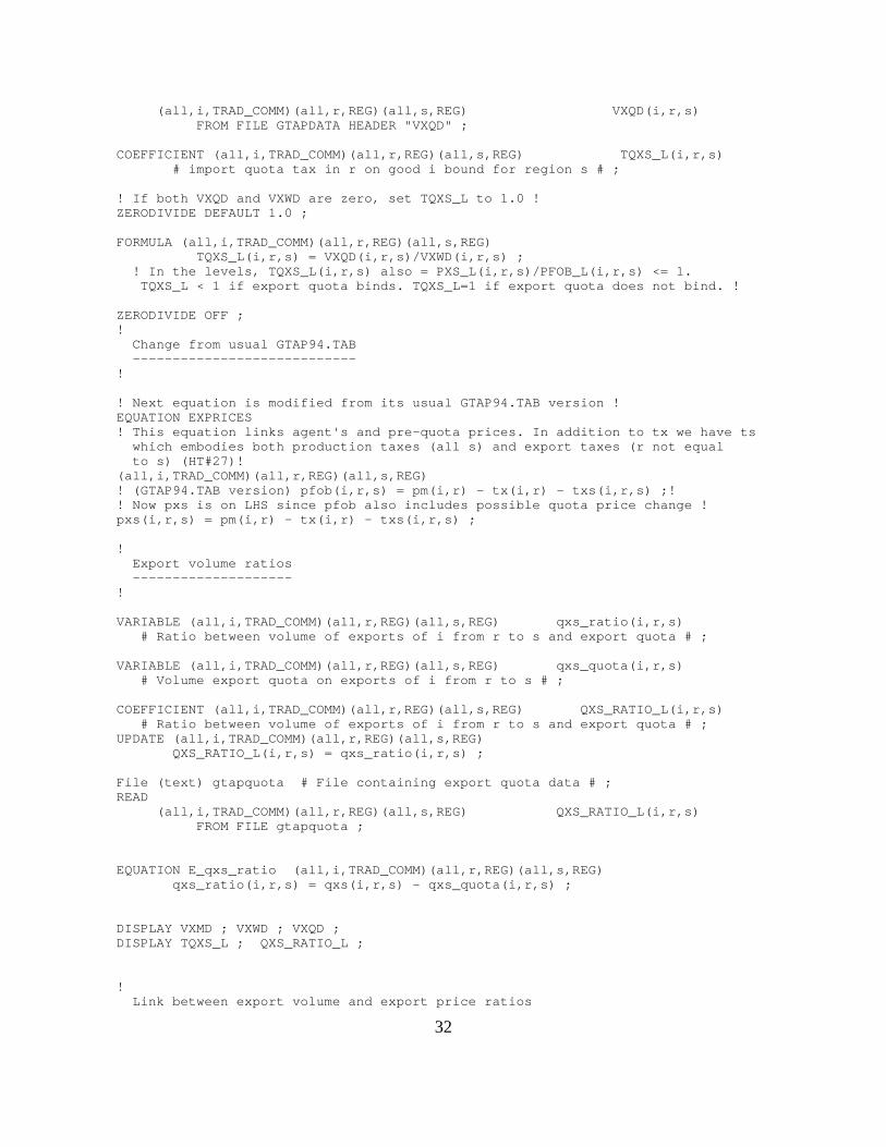
This shows the additions to the standard GTAP94.TAB file for bilateral export quotas. Youcan find these additions at the end of the file GTAP33XQ.TAB used in Examples A1-A6 andP1-P2. The only part of GTAP94.TAB which is changed is the EXPRICES equation, theoriginal version of which is replaced by the version shown below. [More specifically,GTAP33XQ.TAB is based on version 2a August 1995 of GTAP94.TAB.]

[In the export quota example above in section 2 of the paper, bilateral export quotas were onlyadded for certain commodities (the MFA commodities) from certain regions (the MFA-exporting regions) to other specified regions (the MFA-importing regions). This requiresslightly more complicated additions to distinguish these different sets. You can see theTABLO statements added to GTAP94.TAB for the example in section 2 of the paper bylooking at the file MFA-XQ.TAB which you should find amongst the associated computerfiles -see Appendix 1.]

! ----------------------------------------------------------------------- !! Additions for bilateral volume export quotas !! ----------------------------------------------------------------------- !

! Export price ratios -------------------!

VARIABLE (all,i,TRAD_COMM)(all,r,REG)(all,s,REG) pxs(i,r,s) # price of commodity i supplied from r to s inclusive of export taxes # ; ! May be less than pfob(i,r,s) in the levels if the export quota on i from r to s is binding !

VARIABLE (all,i,TRAD_COMM)(all,r,REG)(all,s,REG) tqxs(i,r,s) # import quota tax in r on good i bound for region s # ; ! In the levels, TQXS_L(i,r,s) = PXS_L(i,r,s)/PFOB_L(i,r,s) <= 1. TQXS_L < 1 if export quota binds. TQXS_L=1 if export quota does not bind. !

EQUATION E_tqxs (all,i,TRAD_COMM)(all,r,REG)(all,s,REG) tqxs(i,r,s) = pxs(i,r,s) - pfob(i,r,s) ;

COEFFICIENT (all,i,TRAD_COMM)(all,r,REG)(all,s,REG) VXQD(i,r,s) ! exports of commodity i from region r to destination s valued prior to any quota rent (tradeables only). This value includes export taxes ! ;UPDATE (all,i,TRAD_COMM)(all,r,REG)(all,s,REG) VXQD(i,r,s) = pxs(i,r,s) * qxs(i,r,s) ;

READ

32

(all,i,TRAD_COMM)(all,r,REG)(all,s,REG) VXQD(i,r,s) FROM FILE GTAPDATA HEADER "VXQD" ;

COEFFICIENT (all,i,TRAD_COMM)(all,r,REG)(all,s,REG) TQXS_L(i,r,s) # import quota tax in r on good i bound for region s # ;

! If both VXQD and VXWD are zero, set TQXS_L to 1.0 !ZERODIVIDE DEFAULT 1.0 ;

FORMULA (all,i,TRAD_COMM)(all,r,REG)(all,s,REG) TQXS_L(i,r,s) = VXQD(i,r,s)/VXWD(i,r,s) ; ! In the levels, TQXS_L(i,r,s) also = PXS_L(i,r,s)/PFOB_L(i,r,s) <= 1. TQXS_L < 1 if export quota binds. TQXS_L=1 if export quota does not bind. !

ZERODIVIDE OFF ;! Change from usual GTAP94.TAB ----------------------------!

! Next equation is modified from its usual GTAP94.TAB version !EQUATION EXPRICES! This equation links agent's and pre-quota prices. In addition to tx we have ts which embodies both production taxes (all s) and export taxes (r not equal to s) (HT#27)!(all,i,TRAD_COMM)(all,r,REG)(all,s,REG)! (GTAP94.TAB version) pfob(i,r,s) = pm(i,r) - tx(i,r) - txs(i,r,s) ;!! Now pxs is on LHS since pfob also includes possible quota price change !pxs(i,r,s) = pm(i,r) - tx(i,r) - txs(i,r,s) ;

! Export volume ratios --------------------!

VARIABLE (all,i,TRAD_COMM)(all,r,REG)(all,s,REG) qxs_ratio(i,r,s) # Ratio between volume of exports of i from r to s and export quota # ;

VARIABLE (all,i,TRAD_COMM)(all,r,REG)(all,s,REG) qxs_quota(i,r,s) # Volume export quota on exports of i from r to s # ;

COEFFICIENT (all,i,TRAD_COMM)(all,r,REG)(all,s,REG) QXS_RATIO_L(i,r,s) # Ratio between volume of exports of i from r to s and export quota # ;UPDATE (all,i,TRAD_COMM)(all,r,REG)(all,s,REG) QXS_RATIO_L(i,r,s) = qxs_ratio(i,r,s) ;

File (text) gtapquota # File containing export quota data # ;READ (all,i,TRAD_COMM)(all,r,REG)(all,s,REG) QXS_RATIO_L(i,r,s) FROM FILE gtapquota ;

EQUATION E_qxs_ratio (all,i,TRAD_COMM)(all,r,REG)(all,s,REG) qxs_ratio(i,r,s) = qxs(i,r,s) - qxs_quota(i,r,s) ;

DISPLAY VXMD ; VXWD ; VXQD ;DISPLAY TQXS_L ; QXS_RATIO_L ;

! Link between export volume and export price ratios

33

--------------------------------------------------!

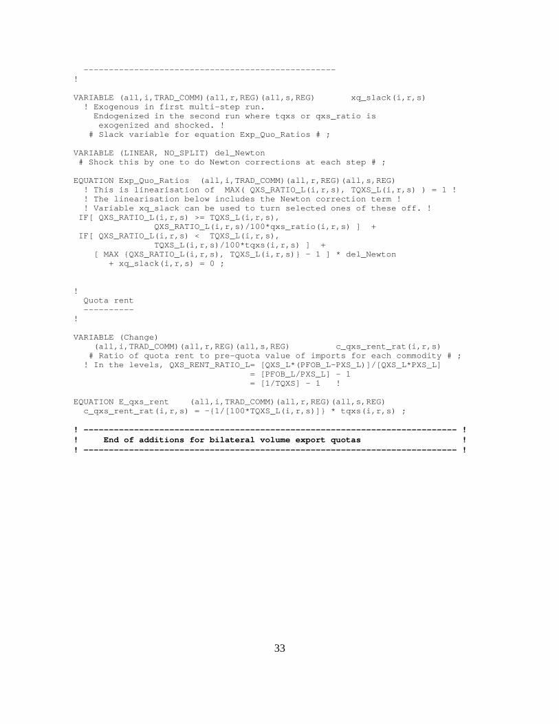
VARIABLE (all,i,TRAD_COMM)(all,r,REG)(all,s,REG) xq_slack(i,r,s) ! Exogenous in first multi-step run. Endogenized in the second run where tqxs or qxs_ratio is exogenized and shocked. ! # Slack variable for equation Exp_Quo_Ratios # ;

VARIABLE (LINEAR, NO_SPLIT) del_Newton # Shock this by one to do Newton corrections at each step # ;

EQUATION Exp_Quo_Ratios (all,i,TRAD_COMM)(all,r,REG)(all,s,REG) ! This is linearisation of MAX( QXS_RATIO_L(i,r,s), TQXS_L(i,r,s) ) = 1 ! ! The linearisation below includes the Newton correction term ! ! Variable xq_slack can be used to turn selected ones of these off. ! IF[ QXS_RATIO_L(i,r,s) >= TQXS_L(i,r,s), QXS_RATIO_L(i,r,s)/100*qxs_ratio(i,r,s) ] + IF[ QXS_RATIO_L(i,r,s) < TQXS_L(i,r,s), TQXS_L(i,r,s)/100*tqxs(i,r,s) ] + [ MAX {QXS_RATIO_L(i,r,s), TQXS_L(i,r,s)} - 1 ] * del_Newton + xq_slack(i,r,s) = 0 ;

! Quota rent ----------!

VARIABLE (Change) (all,i,TRAD_COMM)(all,r,REG)(all,s,REG) c_qxs_rent_rat(i,r,s) # Ratio of quota rent to pre-quota value of imports for each commodity # ; ! In the levels, QXS_RENT_RATIO_L= [QXS_L*(PFOB_L-PXS_L)]/[QXS_L*PXS_L] = [PFOB_L/PXS_L] - 1 = [1/TQXS] - 1 !

EQUATION E_qxs_rent (all,i,TRAD_COMM)(all,r,REG)(all,s,REG) c_qxs_rent_rat(i,r,s) = -{1/[100*TQXS_L(i,r,s)]} * tqxs(i,r,s) ;

! -------------------------------------------------------------------------- !! End of additions for bilateral volume export quotas !! -------------------------------------------------------------------------- !

34

Appendix 3: Linearizing the Exp_Quo_Ratios Levels

Equations for Quotas

Here we show how this is done in the bilateral export quotas case. Other cases are similar.

The relevant equation is the Exp_Quo_Ratios equation (see equation L4 in section 2 above),namely

MAX [ QXS_RATIO(i,r,s)_L, TQXS_L(i,r,s) ] = 1 (L4)

In this section we abbreviate

• QXS_RATIO_L(i,r,s) as QR (quantity ratio) and

• TQXS_L(i,r,s) as PR (price ratio - it is the ratio of PXS and PFOB - see section 2).

Linearizing MAX(QR,PR)=1

The equation "MAX(QR,PR)=1" must be put as a linearized EQUATION on the TABLOInput file since, at present, TABLO Input files do not allow the function MAX to appear inLEVELS EQUATIONs.

When considering MAX(QR,PR), there are two cases.

(a) If QR >= PR, then MAX(QR,PR)=QR so that the change in MAX(QR,PR) is equal to thechange in QR.

(b) If PR > QR, then MAX(QR,PR)=PR so that the change in MAX(QR,PR) is equal to thechange in PR.

Combining these two into one equation using "IF" we can say that

change in MAX(QR,PR) = IF(QR >= PR, c_QR) + IF(QR < PR, c_PR)

where c_QR and c_PR denote the changes in QR and PR. Thus we can use

IF(QR >= PR, c_QR) + IF(QR < PR, c_PR) = 0

as the linearization of the equation MAX(QR,PR)=1.

If QR and PR have associated percent change linear variables p_QR and p_PR in the model,this becomes

IF(QR >= PR, QR/100*p_QR) + IF(QR < PR, PR/100*p_PR) = 0.

35

In the GTAP case,

QR = QXS_RATIO_L(i,r,s) so that p_QR is just the linear variable qxs_quota(i,r,s).

PR = TQXS_L(i,r,s) so that p_PR is just the linear variable tqxs(i,r,s).

Thus, the linearized equation Exp_Quo_Ratios might be written as

EQUATION Exp_Quo_Ratios (all,i,TRAD_COMM)(all,r,REG)(all,s,REG)! This is linearization of MAX( QXS_RATIO_L(i,r,s), TQXS_L(i,r,s) ) = 1 ! IF[ QXS_RATIO_L(i,r,s) >= TQXS_L(i,r,s), QXS_RATIO_L(i,r,s)/100*qxs_ratio(i,r,s) ] + IF[ QXS_RATIO_L(i,r,s) < TQXS_L(i,r,s), TQXS_L(i,r,s)/100*tqxs(i,r,s) ] = 0 ;

In fact the actual equation has two other terms (see Appendix 2 above). One of these terms isthe slack variable xq_slack(i,r,s). This term is added so that, for selected (i,r,s), thesevariables can be set endogenous, which effectively turns this equation off for these (i,r,s). Thisis done in the second accurate simulation (see sections 3.6 and 8 above).

The other term in the Exp_Quo_Ratios equation shown in Appendix 2 involves the variabledel_Newton. This is introduced to implement the so-called Newton correction when runninga multi-step calculation. Roughly, the idea of this Newton correction term is to make sure thatthe two ratios QR and PR return to no larger than 1.0 if they ever get larger than that (as theysometimes will in a multi-step calculation). More details about this are given below.

Linearizing MAX(QR,PR)=1 with Newton Correction

Although the linearization above will produce fairly accurate multi-step solutions provided avery large number of steps is taken, more accurate solutions with fewer steps can be obtainedusing Newton corrections, which are described below, first in general terms, and then as theyapply to our MAX(QR,PR)=1 equation.

For an equation

A = 0

the Newton correction is to handle the case where (during a multistep calculation, say) wehave wandered off the curve so that the current levels value of A is not zero but has the valueE (error) say. Thus we rewrite the equation as

A = E.

The change linearization of this is

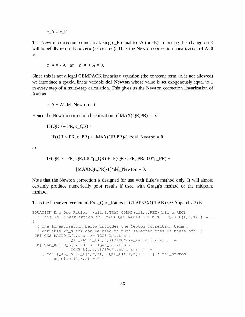
36

c_A = c_E.

The Newton correction comes by taking c_E equal to -A (or -E). Imposing this change on Ewill hopefully return E to zero (as desired). Thus the Newton correction linearization of A=0is

c_A = - A or c_A + A = 0.

Since this is not a legal GEMPACK linearized equation (the constant term -A is not allowed)we introduce a special linear variable del_Newton whose value is set exogenously equal to 1in every step of a multi-step calculation. This gives us the Newton correction linearization ofA=0 as

c_A + A*del_Newton = 0.

Hence the Newton correction linearization of MAX(QR,PR)=1 is

IF(QR >= PR, c_QR) +

IF(QR < PR, c_PR) + [MAX(QR,PR)-1]*del_Newton = 0.

or

IF(QR >= PR, QR/100*p_QR) + IF(QR < PR, PR/100*p_PR) +

[MAX(QR,PR)-1]*del_Newton = 0.

Note that the Newton correction is designed for use with Euler's method only. It will almostcertainly produce numerically poor results if used with Gragg's method or the midpointmethod.

Thus the linearized version of Exp_Quo_Ratios in GTAP33XQ.TAB (see Appendix 2) is

EQUATION Exp_Quo_Ratios (all,i,TRAD_COMM)(all,r,REG)(all,s,REG) ! This is linearization of MAX( QXS_RATIO_L(i,r,s), TQXS_L(i,r,s) ) = 1! ! The linearization below includes the Newton correction term ! ! Variable xq_slack can be used to turn selected ones of these off. ! IF[ QXS_RATIO_L(i,r,s) >= TQXS_L(i,r,s), QXS_RATIO_L(i,r,s)/100*qxs_ratio(i,r,s) ] + IF[ QXS_RATIO_L(i,r,s) < TQXS_L(i,r,s), TQXS_L(i,r,s)/100*tqxs(i,r,s) ] + [ MAX {QXS_RATIO_L(i,r,s), TQXS_L(i,r,s)} - 1 ] * del_Newton + xq_slack(i,r,s) = 0 ;

37

Note that the variable del_Newton is declared in the TABLO Input file via the statement

VARIABLE (LINEAR, NO_SPLIT) del_Newton # Shock this by one to do Newton corrections at each step #

;

The qualifier "NO_SPLIT" is a previously-undocumented VARIABLE qualifier. It means thatany shock given to the variable will be given in each step of a multi-step calculation (ratherthan being spread out across all steps as usual). Variable del_Newton should always be set asexogenous. Usually it is shocked by one (always in the first approximate quota simulation).However it does not need to be shocked in the second (accurate) quota simulations. (Shockingit should make no noticeable difference to the results, except for any components of xq_slackwhich are endogenous.)