Implications of Climate Science for PolicyHenry D. Jacoby

Climate Policy Note No. 2July 2013

The MIT Joint Program on the Science and Policy of Global Change is an organization for research, independent policy analysis, and public education in global environmental change. It seeks to provide leadership in understanding scientific, economic, and ecological aspects of this difficult issue, and combining them into policy assessments that serve the needs of ongoing national and international discussions. To this end, the Program brings together an interdisciplinary group from two established research centers at MIT: the Center for Global Change Science (CGCS) and the Center for Energy and Environmental Policy Research (CEEPR). These two centers bridge many key areas of the needed intellectual work, and additional essential areas are covered by other MIT departments, by collaboration with the Ecosystems Center of the Marine Biology Laboratory (MBL) at Woods Hole, and by short- and long-term visitors to the Program. The Program involves sponsorship and active participation by industry, government, and non-profit organizations.

To inform processes of policy development and implementation, climate change research needs to focus on improving the prediction of those variables that are most relevant to economic, social, and environmental effects. In turn, the greenhouse gas and atmospheric aerosol assumptions underlying climate analysis need to be related to the economic, technological, and political forces that drive emissions, and to the results of international agreements and mitigation. Further, assessments of possible societal and ecosystem impacts, and analysis of mitigation strategies, need to be based on realistic evaluation of the uncertainties of climate science.

Ronald G. Prinn and John M. ReillyProgram Co-Directors

For more information, please contact the Joint Program Office Postal Address: Joint Program on the Science and Policy of Global Change 77 Massachusetts Avenue MIT E19-411 Cambridge MA 02139-4307 (USA) Location: 400 Main Street, Cambridge Building E19, Room 411 Massachusetts Institute of Technology Access: Phone: +1.617. 253.7492 Fax: +1.617.253.9845 E-mail: globalchange@mit.edu Web site: http://globalchange.mit.edu/

Printed on recycled paper

1

Implications of Climate Science for Policy

Henry D. Jacoby*†

Abstract

Climate change presents the greatest challenge ever faced by our domestic and international

institutions, and a great deal of the difficulty lies in the science of the issue. Because human influence

on global climate differs in important ways from other environmental threats these peculiarities set

the context for discussion of what can be done to reduce greenhouse gas emissions and to adapt to

change that cannot be avoided. Following a brief summary of current understanding of how Earth’s

climate works, five ways are presented by which the science of climate impinges on attempts to

construct a policy response.

Contents

1. THE CLIMATE CHALLENGE ....................................................................................................1 1.1 Origins of the Science of Earth’s Climate ............................................................................2 1.2 Where the Science Impinges on Policy ................................................................................3

2. HOW OUR CLIMATE SYSTEM WORKS .................................................................................4 2.1 The Earth, the Sun and the Greenhouse Effect .....................................................................4 2.2 Agents Forcing the Climate ..................................................................................................5

2.2.1 Carbon Dioxide and the Carbon Cycle ......................................................................5 2.2.2 Non-CO2 Gases ..........................................................................................................7 2.2.3 The Magnitude of Natural and Human Forcings .......................................................8

2.3 The Role of the Ocean ..........................................................................................................9 2.4 Feedbacks with Rising Temperature .................................................................................. 11

3. WHERE ARE WE NOW, AND WHERE ARE WE HEADED? ............................................... 12 4. WHERE THE SCIENCE IMPINGES ON POLICY ACTION ................................................... 14

4.1 Contradicts Common Mental Models of System Behavior ................................................ 14 4.2 Requires Attention to Multiple, Diverse, Poorly Measured Influences .............................. 15 4.3 Demands Cooperative Effort by Parties with Diverse Interests ......................................... 17 4.4 Reveals Uncertainty that Complicates Mitigation Decision ............................................... 19 4.5 Creates Special Difficulty in Formulating Adaptation Measures ....................................... 22

5. COMBINED EFFECTS ON THE CHOICE OF RESPONSE STRATEGY .............................. 23 6. REFERENCES ............................................................................................................................ 24

1. THE CLIMATE CHALLENGE

Societies have been dealing with environmental threats for centuries, each problem presenting

its own set of institutional difficulties. Managing human influence on the Planet’s climate

presents a challenge beyond any confronted before, however, and the roots of the difficulty lie in

the underlying science of the issue. Here we review our understanding of how the Earth system

works and ways our activity is influencing it, and explore the reasons why the issue so severely

challenges the mental capability developed in human evolution and the political institutions

developed along the way.

* Joint Program on the Science and Policy of Global Change, Massachusetts Institute of Technology, Cambridge,

MA. † Corresponding author (hjacoby@mit.edu).

2

1.1 Origins of the Science of Earth’s Climate

Knowledge of the threat of climate change, and the policy challenges it presents, are founded

mainly on scientific calculation. There is anecdotal evidence in our day-to-day experience that

changes projected by scientific analysis are already taking place—for example in the earlier

flowering of plants in some parts of the world, changes in migration patterns of birds, and

increases in record high temperatures and intense storms. Also, thermometer and other

measurements show an increase in global temperature over the past 150 years, but even these

estimates require scientific analysis to convert widely distributed and sometimes sparse

measurements into a global picture. Looking forward, projection of the response of the climate to

human intervention is wholly a matter of research on the complicated interactions within the

earth system, and simulation in computer models.

So where does this knowledge base come from? The history is a long one, dating at least to

the early 19th

century when Jean Baptiste Joseph Fourier, the great French mathematician and

physical scientist, calculated that, given its distance from the Sun, the Earth should be cooler

than it is. Among his hypotheses was the possibility that something in the atmosphere was acting

as an insulator. Discovery of the cause came with the work of the Irish scientist John Tyndall

who in 1861 showed that water vapor and CO2 can trap radiant energy. Then in 1896 a Swedish

scientist, Svante Arrhenius, who was seeking to understand what caused the ice ages, concluded

that the CO2 added to the atmosphere could raise global temperature. He computed that a

doubling of its atmospheric concentration would yield a 4°C increase, an estimate somewhat

higher than current calculations but amazingly close considering the climate system knowledge

and computation facilities at his disposal. One forecast Arrhenius got wrong: based on his

expectation for the emerging industrial age and the absorption of CO2 in the Earth system he

thought it would take several thousand years to burn enough fossil fuels to yield an atmospheric

doubling. In fact we are on a track to pass that milestone in the next few decades.

During World War II substantial advances were made in meteorology, and in following

decades the computer revolution produced dramatic increases in the capacity for numerical

calculation. Over time, facilities developed originally for numerical weather forecasting were

extended to longer-term climate projections; eventually these were coupled to models of ocean

behavior; and still later representations were added of the influence of the terrestrial biosphere.

Also, governments supported growing programs of earth observations to support this research

and analysis, so that by the turn of the 21st century several billion U.S. dollars per year were

being spent on climate research and observation in the U.S., Europe, Japan, Australia and several

other countries.

This activity gained a major push in the 1970s when environmental threats were gaining

greater salience in many countries, and summaries of then-current scientific knowledge

supported the expectation that human emissions were at levels that could change the climate. In

the U.S., for example, the so-called Charney Report commissioned by the President’s Office of

Science and Technology Policy (US NAS, 1979) played an important role in raising concern

about the issue and increasing public and policymaker confidence in the ability of the emerging

3

science to understand it. By the late 1990s political concern with the issue was rising and, to gain

some coherence and quality control in the information being developed, governments created the

Intergovernmental Panel on Climate Change (IPCC) with the task of periodically summarizing

the research and analysis.

As of this writing work on the science of climate has spread around the world, and the IPCC

is near completion of its Fifth Assessment Report (the AR-5). The science volume of the AR-5

will summarize results of climate projections by over a dozen large-scale models from the U.S.,

EU, Japan and Australia. The most complete of these models—the atmospheric-ocean general

circulation models—are among of the largest numerical calculations ever attempted. Not

surprisingly considering the complexity of the earth system, these efforts yield different

projection of future climate, and even the spread among the models does not fully reflect the

uncertainty. Thus in exploring the implications of the climate science for policy we are talking in

the main about knowledge developed in these research and analysis activities, and the earth

observation systems that underlie them, and about the level of understanding of this work among

the media, political leaders and the public.

1.2 Where the Science Impinges on Policy

Five characteristics of the issue can be identified that are particularly important in

conditioning potential responses to the threat—either by reducing greenhouse emissions and

other influences or by taking measures to ease adaptation to change that cannot be avoided:

Scientific understanding of the planet contradicts our common mental model of

environmental threats.

There is not just one source of the climate change threat. Many and varied types of

activities contribute to the human influence and some are hard to measure.

Reduction of the threat requires emissions mitigation by many nations, rich and poor,

creating a “commons” problem more complex than the world has confronted before.

Uncertainty in scientific analysis of the response of global climate to greenhouse

emissions complicates the process of deciding mitigation action.

The effects of climate change at the local level are even more uncertain than at a global

scale, yet it is at the local and regional levels where adaptation takes place.

In combination they present a challenge that thus far is proving to be beyond the coping capacity

of our national and international institutions.

To see the depth of the problem, consider a comparison with another familiar environmental

insult: health issues from the pollution of surface waters by human waste. We understand the

main source of the problem—the sewer outflow of urban areas—and we have developed ways to

allocate the cleanup cost in a politically acceptable manner. Moreover, we understand pretty well

what will happen to stream quality if various treatment methods are applied. And finally,

conditions at local scale are not hard to predict, and effects of adaptation to any residual risk

(e.g., boiling water, purchase of bottled water) are easy to understand. It is not that these issues

4

present no challenges to private decisions and public institutions, but what problems as there are

do not reside in the science of water pollution.

We will return to these peculiar aspects of the climate threat, but first it is useful to work

through a brief summary of current scientific understanding of how our planet works, to prepare

a shared base of knowledge of system function and the terminology use to describe it.1

2. HOW OUR CLIMATE SYSTEM WORKS

2.1 The Earth, the Sun and the Greenhouse Effect

At the most fundamental level our climate is determined by the Earth’s relationship to the

Sun. Energy comes in from the Sun and is radiated back to space, and if these two are in balance

the global temperature will be constant. If the energy sent out is less than that coming in the

planet will warm, and vice versa. It’s as simple as that at one level: human-emitted greenhouse

gases hold more of the incoming energy in the system.

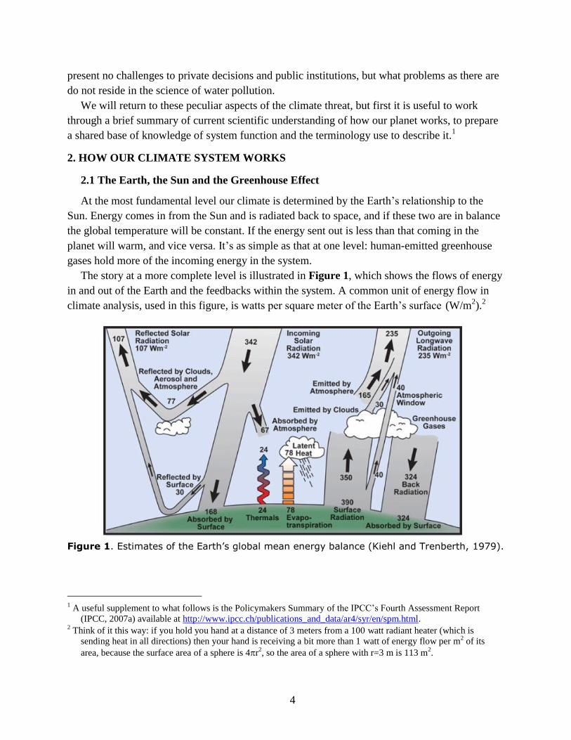
The story at a more complete level is illustrated in Figure 1, which shows the flows of energy

in and out of the Earth and the feedbacks within the system. A common unit of energy flow in

climate analysis, used in this figure, is watts per square meter of the Earth’s surface (W/m2).

2

Figure 1. Estimates of the Earth’s global mean energy balance (Kiehl and Trenberth, 1979).

1 A useful supplement to what follows is the Policymakers Summary of the IPCC’s Fourth Assessment Report

(IPCC, 2007a) available at http://www.ipcc.ch/publications_and_data/ar4/syr/en/spm.html. 2 Think of it this way: if you hold you hand at a distance of 3 meters from a 100 watt radiant heater (which is

sending heat in all directions) then your hand is receiving a bit more than 1 watt of energy flow per m2 of its

area, because the surface area of a sphere is 4r2, so the area of a sphere with r=3 m is 113 m

2.

5

The figure shows the Earth in balance with the sun and outer space, with these exchanges shown

across the top of the figure. Incoming solar radiation, mainly at short wave lengths, is 342 W/m2,

and this is balanced by 107 W/m2

reflected to space at its original wavelengths, some from

clouds and some from the surface, and 235 W/m2 outgoing as longwave (infrared) radiation.

Longwave radiation is given off by any warm body (the phenomenon exploited by the night

scope on a soldier’s weapon).

The key to a livable planet is shown in the right hand part of the figure. While reflected solar

radiation passes back out of the system without interacting with molecules in the atmosphere, the

longwave radiation does interact, reflecting 324 W/m2

back to the surface. The most important of

these substances is water vapor, but also significant even in this picture of balance is a set of

other natural greenhouses (GHGs) such as CO2, methane, nitrous oxide and others to be

discussed below. Now enter humans. We contribute additional volumes of the natural GHGs plus

some we have invented, which has the effect of augmenting the 324 W/m2 back radiation in the

figure. More trapped heat warms the planet until the hotter surface augments the previous

outflow of longwave radiation to space by enough to restore balance.

Then there are additional phenomena that can be discussed using this figure. Human activity

affects the reflection of solar radiation in two ways. White aerosols—mainly sulfate particles

formed from sulfur emissions of coal-fired powerplants—increase reflection, with a cooling

influence. Humans influence the reflectivity of the surface, its so-called albedo, by changes in

land use and by cutting the reflectivity of snow and ice by dirtying it with soot, which is

produced mainly by diesel engines and biomass burning. Not shown in the figure is another

influence: black aerosols which absorb radiation, warming the atmosphere. The combined

influence of these various effects is commonly referred to the anthropogenic “forcing” of the

climate, also in W/m2.

Also to be noted while looking at Figure 1 are positive feedbacks that accompany warming of

the planet, to be discussed later. Warmer ocean and atmospheric temperatures lead to loss of

snow and ice, which lowers the reflection of solar radiation from the surface, and aerosols have

an effect on cloud formation, which influences their complex role in the energy budget. And,

most important, a warmer atmosphere will hold more water vapor, increasing the power of the

most important of the greenhouse substances.

2.2 Agents Forcing the Climate

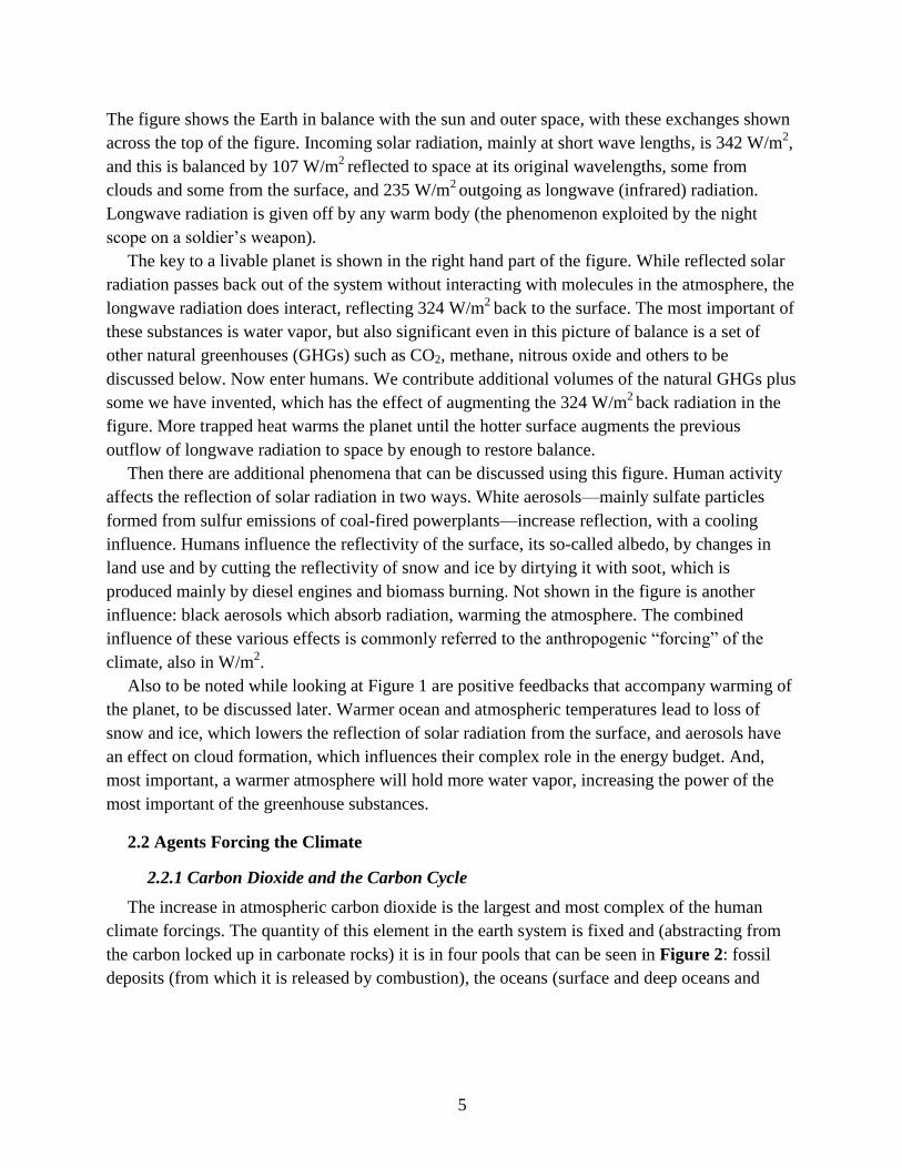
2.2.1 Carbon Dioxide and the Carbon Cycle

The increase in atmospheric carbon dioxide is the largest and most complex of the human

climate forcings. The quantity of this element in the earth system is fixed and (abstracting from

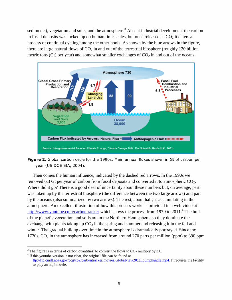
the carbon locked up in carbonate rocks) it is in four pools that can be seen in Figure 2: fossil

deposits (from which it is released by combustion), the oceans (surface and deep oceans and

6

sediments), vegetation and soils, and the atmosphere.3 Absent industrial development the carbon

in fossil deposits was locked up on human time scales, but once released as CO2 it enters a

process of continual cycling among the other pools. As shown by the blue arrows in the figure,

there are large natural flows of CO2 in and out of the terrestrial biosphere (roughly 120 billion

metric tons (Gt) per year) and somewhat smaller exchanges of CO2 in and out of the oceans.

Figure 2. Global carbon cycle for the 1990s. Main annual fluxes shown in Gt of carbon per

year (US DOE EIA, 2004).

Then comes the human influence, indicated by the dashed red arrows. In the 1990s we

removed 6.3 Gt per year of carbon from fossil deposits and converted it to atmospheric CO2.

Where did it go? There is a good deal of uncertainty about these numbers but, on average, part

was taken up by the terrestrial biosphere (the difference between the two large arrows) and part

by the oceans (also summarized by two arrows). The rest, about half, is accumulating in the

atmosphere. An excellent illustration of how this process works is provided in a web video at

http://www.youtube.com/carbontracker which shows the process from 1979 to 2011.4 The bulk

of the planet’s vegetation and soils are in the Northern Hemisphere, so they dominate the

exchange with plants taking up CO2 in the spring and summer and releasing it in the fall and

winter. The gradual buildup over time in the atmosphere is dramatically portrayed. Since the

1770s, CO2 in the atmosphere has increased from around 270 parts per million (ppm) to 390 ppm

3 The figure is in terms of carbon quantities: to convert the flows to CO2 multiply by 3.6.

4 If this youtube version is not clear, the original file can be found at

ftp://ftp.cmdl.noaa.gov/ccg/co2/carbontracker/movies/Globalview2011_pumphandle.mp4. It requires the facility

to play an mp4 movie.

7

today. The video goes on to plot the CO2 levels back in time for several hundred thousand years

using data from ice cores and other sources. The CO2 levels are correlated with temperature, so

the path roughly traces the ice ages and warm periods of the distant past.

Figure 2, also highlights a fact about this greenhouse gas to which we will return later: its

“stock pollutant” nature. It can be illustrated by the following calculation, which is not exact

given the complexities of the carbon cycle but nonetheless informative. We have added 160 to

170 GtC as of the 1990s. If all human emissions were halted immediately, at what rate would the

system return to its earlier state? Answer: the oceans and terrestrial biosphere would begin to

remove the carbon at a rate of only around 4 GtC per year. Thus the climate influence of change

already made to the planet will continue for a very long time, even under the fantasy that we

could halt all global emissions immediately.

2.2.2 Non-CO2 Gases

Many gases can trap longwave energy, but the primary ones are listed in Table 1. Most are

present in nature, but are augmented by industrial and farming activities. The most important is

methane, which is released in fossil energy production and by agricultural activities that create

conditions for methane-producing bacteria such as rice growing, releases from the intestines of

ruminant animals like cows and sheep, and manure management. Another important source of

methane is leakage from natural gas pipelines and consumer appliances. Nitrous oxide also is

released in fossil combustion and in some industrial activities, but has its main source in

agriculture where nitrogen fertilizer stimulates the activity of other bacteria that produce this gas.

Table 1. Non-CO2 Greenhouse Contributors.

Sources Sinks

Primary warming effects

Methane (CH4) Biogenic, fossil Destruction by OH

Nitrous Oxide (N2O) Biogenic, industrial UV radiation

Sulfur Hexafluoride (SF6) Industrial, natural Extremely stable

Hydrofleurocarbons

(HFCs & HCFCs) Industrial, natural Destruction by OH

Perfleurocarbon (PFCs) Industrial, natural Extremely stable

Black carbon (aerosols) Fossil, biofuels, dust Deposition

Knock-on warming

effects

Ozone (O3) Fossil Photochemistry

Cooling effects

Sulfate aerosol (SO2) Fossil Deposition

Then there are the industrial gases—HFCs and HCFCs used in air conditioning and various

solvent applications, PFCs which are a byproduct of aluminum processing and are also

8

manufactured for use in the electronics industry and other applications, and SF6 which is used

mainly as an insulator in electric transformers.5

Also shown in the table are the aerosols mentioned earlier, both the warming black aerosols

and the reflecting sulfate aerosols that have a cooling effect. Then there is ozone, another

greenhouse gas, which is emitted directly in infinitesimal quantities by human activity but is

produced in the atmosphere by chemical action of two by-products of fossil fuel use: organic

compounds from incomplete combustion and methane release, and NOx. (These influences will

show up again below in discussion of mitigation strategies.)

Each of the non-CO2 gases has limited residence time in the atmosphere (see Table 2).

Carbon dioxide, which cycles in and out of the various pools, cannot be said to have a “lifetime”.

At best estimates can be made of the approximate time an emitted molecule spends in the

atmosphere before being absorbed into the terrestrial biosphere or the oceans—generally

estimated to be somewhat over a century. All of the non-CO2 substances, on the other hand, are

subject to some process of chemical destruction or deposition, so lifetimes can be estimated

which range from around a dozen years for methane to thousands of years for some of the

industrial gases.

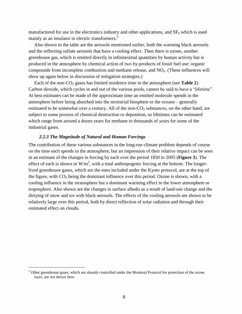
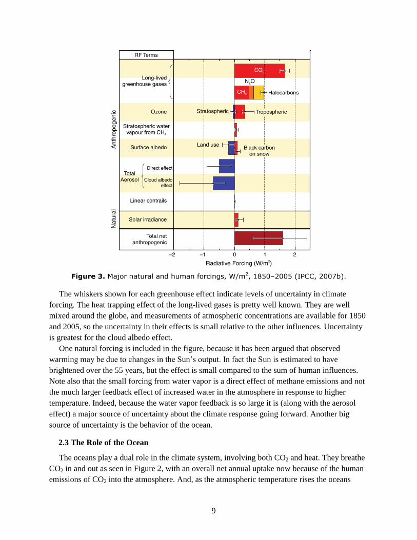
2.2.3 The Magnitude of Natural and Human Forcings

The contribution of these various substances in the long-run climate problem depends of course

on the time each spends in the atmosphere, but an impression of their relative impact can be seen

in an estimate of the changes in forcing by each over the period 1850 to 2005 (Figure 3). The

effect of each is shown in W/m2, with a total anthropogenic forcing at the bottom. The longer-

lived greenhouse gases, which are the ones included under the Kyoto protocol, are at the top of

the figure, with CO2 being the dominant influence over this period. Ozone is shown, with a

cooling influence in the stratosphere but a dominant warming effect in the lower atmosphere or

troposphere. Also shown are the changes in surface albedo as a result of land-use change and the

dirtying of snow and ice with black aerosols. The effects of the cooling aerosols are shown to be

relatively large over this period, both by direct reflection of solar radiation and through their

estimated effect on clouds.

5 Other greenhouse gases, which are already controlled under the Montreal Protocol for protection of the ozone

layer, are not shown here.

9

Figure 3. Major natural and human forcings, W/m2, 1850–2005 (IPCC, 2007b).

The whiskers shown for each greenhouse effect indicate levels of uncertainty in climate

forcing. The heat trapping effect of the long-lived gases is pretty well known. They are well

mixed around the globe, and measurements of atmospheric concentrations are available for 1850

and 2005, so the uncertainty in their effects is small relative to the other influences. Uncertainty

is greatest for the cloud albedo effect.

One natural forcing is included in the figure, because it has been argued that observed

warming may be due to changes in the Sun’s output. In fact the Sun is estimated to have

brightened over the 55 years, but the effect is small compared to the sum of human influences.

Note also that the small forcing from water vapor is a direct effect of methane emissions and not

the much larger feedback effect of increased water in the atmosphere in response to higher

temperature. Indeed, because the water vapor feedback is so large it is (along with the aerosol

effect) a major source of uncertainty about the climate response going forward. Another big

source of uncertainty is the behavior of the ocean.

2.3 The Role of the Ocean

The oceans play a dual role in the climate system, involving both CO2 and heat. They breathe

CO2 in and out as seen in Figure 2, with an overall net annual uptake now because of the human

emissions of CO2 into the atmosphere. And, as the atmospheric temperature rises the oceans

10

absorb heat, in effect creating a “flywheel” effect that introduces a time lag in the effect of the

human forcing. As a result the surface temperature is not yet in equilibrium with the current level

of forcing shown in Figure 3; there is a yet unrealized “commitment” to further change in the

climate even if human forcing were to stay at the current level.

The driver of this process is the deep circulations in the ocean. The top hundred meters or so

is well mixed by wave action, so on a global average this top layer stays in close equilibrium

with the atmosphere in terms of CO2 and temperature. But this top layer alone could not hold the

amount of additional CO2 implied by the estimates in Figure 2, or take up a great amount of heat

in adjusting to a rising atmospheric temperature. The flywheel effect occurs because warm CO2-

rich water is taken from the so-called “mixed” layer and carried into the ocean deeps.

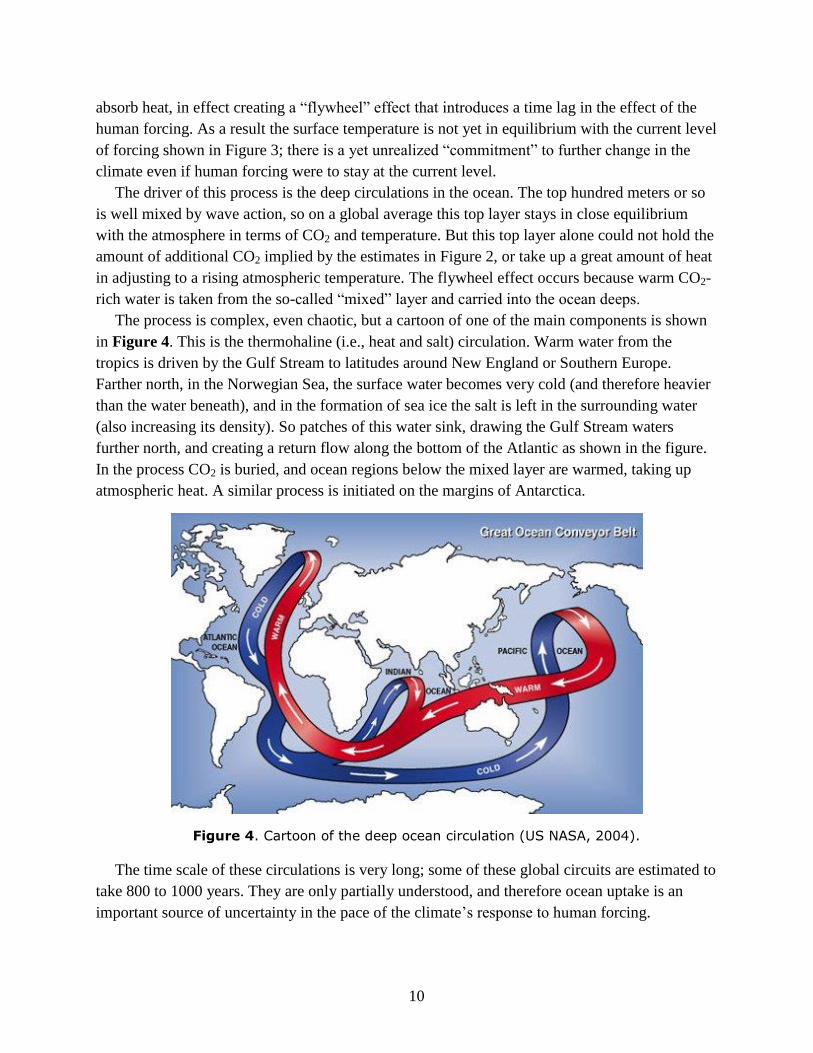
The process is complex, even chaotic, but a cartoon of one of the main components is shown

in Figure 4. This is the thermohaline (i.e., heat and salt) circulation. Warm water from the

tropics is driven by the Gulf Stream to latitudes around New England or Southern Europe.

Farther north, in the Norwegian Sea, the surface water becomes very cold (and therefore heavier

than the water beneath), and in the formation of sea ice the salt is left in the surrounding water

(also increasing its density). So patches of this water sink, drawing the Gulf Stream waters

further north, and creating a return flow along the bottom of the Atlantic as shown in the figure.

In the process CO2 is buried, and ocean regions below the mixed layer are warmed, taking up

atmospheric heat. A similar process is initiated on the margins of Antarctica.

Figure 4. Cartoon of the deep ocean circulation (US NASA, 2004).

The time scale of these circulations is very long; some of these global circuits are estimated to

take 800 to 1000 years. They are only partially understood, and therefore ocean uptake is an

important source of uncertainty in the pace of the climate’s response to human forcing.

11

2.4 Feedbacks with Rising Temperature

If these human forcings were all there was to climate change the threat would be much less

serious than it is. But unfortunately there are a number of system feedbacks to a rise in

temperature, overwhelmingly positive ones that magnify the warming influence. Most important

is the water vapor feedback. At warmer temperatures there is greater evaporation off the oceans,

and a warmer atmosphere will hold more of the resulting water vapor, which is the most

powerful greenhouse influence.

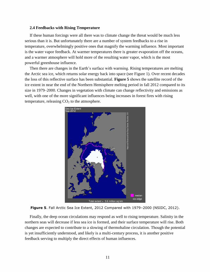
Then there are changes in the Earth’s surface with warming. Rising temperatures are melting

the Arctic sea ice, which returns solar energy back into space (see Figure 1). Over recent decades

the loss of this reflective surface has been substantial. Figure 5 shows the satellite record of the

ice extent in near the end of the Northern Hemisphere melting period in fall 2012 compared to its

size in 1979–2000. Changes in vegetation with climate can change reflectivity and emissions as

well, with one of the more significant influences being increases in forest fires with rising

temperature, releasing CO2 to the atmosphere.

Figure 5. Fall Arctic Sea Ice Extent, 2012 Compared with 1979–2000 (NSIDC, 2012).

Finally, the deep ocean circulations may respond as well to rising temperature. Salinity in the

northern seas will decrease if less sea ice is formed, and their surface temperature will rise. Both

changes are expected to contribute to a slowing of thermohaline circulation. Though the potential

is yet insufficiently understood, and likely is a multi-century process, it is another positive

feedback serving to multiply the direct effects of human influences.

12

3. WHERE ARE WE NOW, AND WHERE ARE WE HEADED?

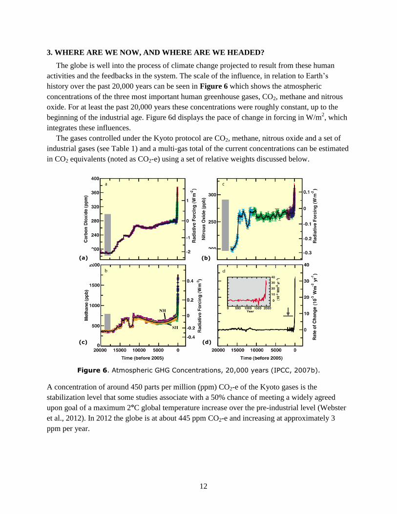
The globe is well into the process of climate change projected to result from these human

activities and the feedbacks in the system. The scale of the influence, in relation to Earth’s

history over the past 20,000 years can be seen in Figure 6 which shows the atmospheric

concentrations of the three most important human greenhouse gases, CO2, methane and nitrous

oxide. For at least the past 20,000 years these concentrations were roughly constant, up to the

beginning of the industrial age. Figure 6d displays the pace of change in forcing in W/m2, which

integrates these influences.

The gases controlled under the Kyoto protocol are CO2, methane, nitrous oxide and a set of

industrial gases (see Table 1) and a multi-gas total of the current concentrations can be estimated

in CO2 equivalents (noted as CO2-e) using a set of relative weights discussed below.

Figure 6. Atmospheric GHG Concentrations, 20,000 years (IPCC, 2007b).

A concentration of around 450 parts per million (ppm) CO2-e of the Kyoto gases is the

stabilization level that some studies associate with a 50% chance of meeting a widely agreed

upon goal of a maximum 2°C global temperature increase over the pre-industrial level (Webster

et al., 2012). In 2012 the globe is at about 445 ppm CO2-e and increasing at approximately 3

ppm per year.

(a) (b)

(c) (d)

13

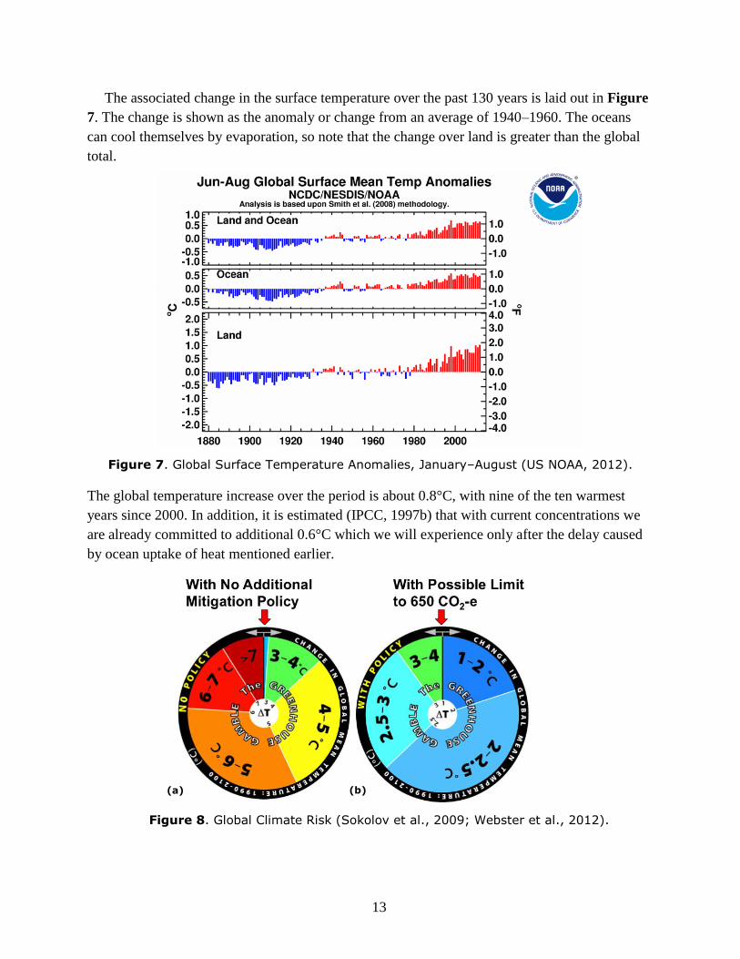
The associated change in the surface temperature over the past 130 years is laid out in Figure

7. The change is shown as the anomaly or change from an average of 1940–1960. The oceans

can cool themselves by evaporation, so note that the change over land is greater than the global

total.

Figure 7. Global Surface Temperature Anomalies, January–August (US NOAA, 2012).

The global temperature increase over the period is about 0.8°C, with nine of the ten warmest

years since 2000. In addition, it is estimated (IPCC, 1997b) that with current concentrations we

are already committed to additional 0.6°C which we will experience only after the delay caused

by ocean uptake of heat mentioned earlier.

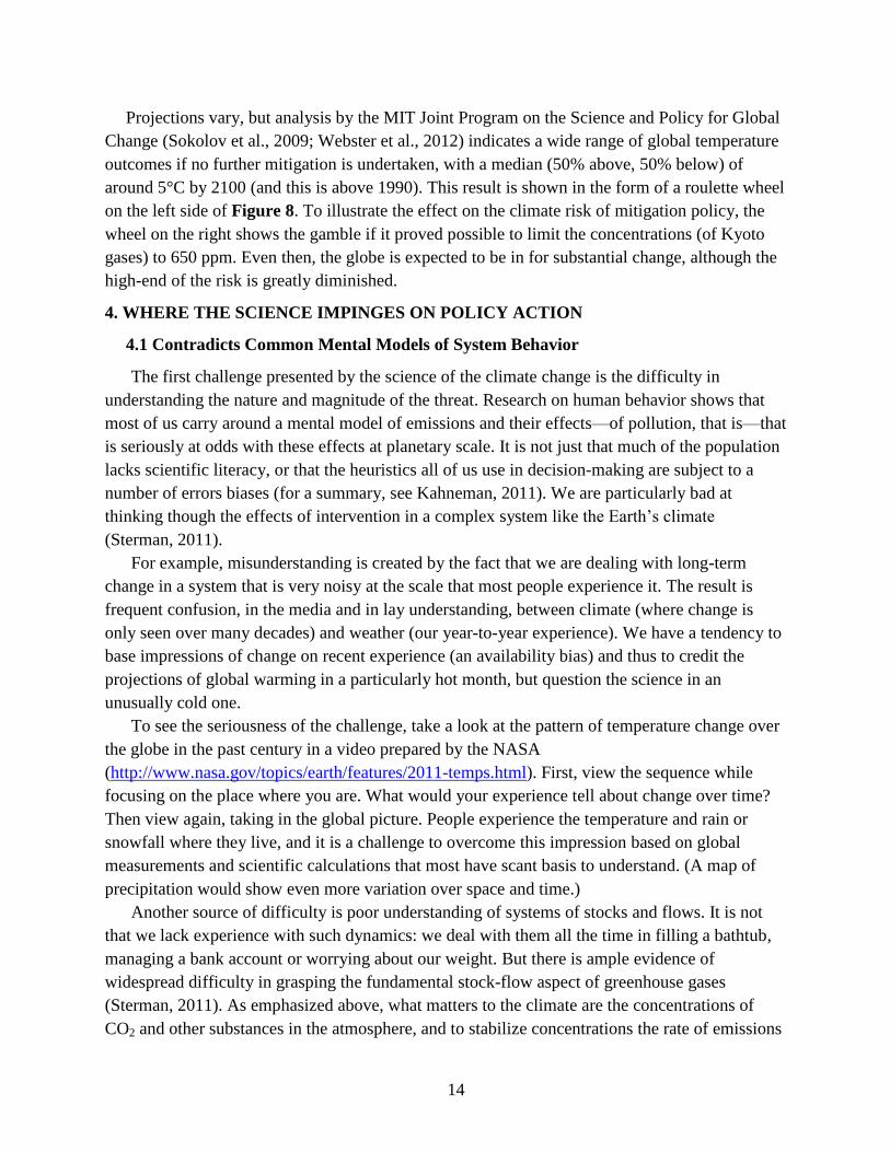
Figure 8. Global Climate Risk (Sokolov et al., 2009; Webster et al., 2012).

(a) (b)

14

Projections vary, but analysis by the MIT Joint Program on the Science and Policy for Global

Change (Sokolov et al., 2009; Webster et al., 2012) indicates a wide range of global temperature

outcomes if no further mitigation is undertaken, with a median (50% above, 50% below) of

around 5°C by 2100 (and this is above 1990). This result is shown in the form of a roulette wheel

on the left side of Figure 8. To illustrate the effect on the climate risk of mitigation policy, the

wheel on the right shows the gamble if it proved possible to limit the concentrations (of Kyoto

gases) to 650 ppm. Even then, the globe is expected to be in for substantial change, although the

high-end of the risk is greatly diminished.

4. WHERE THE SCIENCE IMPINGES ON POLICY ACTION

4.1 Contradicts Common Mental Models of System Behavior

The first challenge presented by the science of the climate change is the difficulty in

understanding the nature and magnitude of the threat. Research on human behavior shows that

most of us carry around a mental model of emissions and their effects—of pollution, that is—that

is seriously at odds with these effects at planetary scale. It is not just that much of the population

lacks scientific literacy, or that the heuristics all of us use in decision-making are subject to a

number of errors biases (for a summary, see Kahneman, 2011). We are particularly bad at

thinking though the effects of intervention in a complex system like the Earth’s climate

(Sterman, 2011).

For example, misunderstanding is created by the fact that we are dealing with long-term

change in a system that is very noisy at the scale that most people experience it. The result is

frequent confusion, in the media and in lay understanding, between climate (where change is

only seen over many decades) and weather (our year-to-year experience). We have a tendency to

base impressions of change on recent experience (an availability bias) and thus to credit the

projections of global warming in a particularly hot month, but question the science in an

unusually cold one.

To see the seriousness of the challenge, take a look at the pattern of temperature change over

the globe in the past century in a video prepared by the NASA

(http://www.nasa.gov/topics/earth/features/2011-temps.html). First, view the sequence while

focusing on the place where you are. What would your experience tell about change over time?

Then view again, taking in the global picture. People experience the temperature and rain or

snowfall where they live, and it is a challenge to overcome this impression based on global

measurements and scientific calculations that most have scant basis to understand. (A map of

precipitation would show even more variation over space and time.)

Another source of difficulty is poor understanding of systems of stocks and flows. It is not

that we lack experience with such dynamics: we deal with them all the time in filling a bathtub,

managing a bank account or worrying about our weight. But there is ample evidence of

widespread difficulty in grasping the fundamental stock-flow aspect of greenhouse gases

(Sterman, 2011). As emphasized above, what matters to the climate are the concentrations of

CO2 and other substances in the atmosphere, and to stabilize concentrations the rate of emissions

15

must be brought down to equal the rate of uptake or destruction. Unfortunately, it is widely

perceived that simply stabilizing emissions will stabilize concentrations. It is a mental model

consistent with other pollution problems—like noise or river pollution—but wrong in this

context.

Related to the stock–flow problem is an incorrect appreciation of the role of time delays in

the system. Two examples will make the point. A common argument in policy discussions, in the

face of uncertainty, is to “wait and learn”. Again, for many environmental issues this is a sound

mental model, because the seriousness of the problem will be roughly the same in a few years

and we may then know better how to deal with it. But it is wrong in this case: for a stock

pollutant the threat does get worse with delay because the stock in the atmosphere is increasing.

Contributing to this problem is poor understanding of ocean circulations, and the time delay they

introduce into climate response to forcing. Because we are committed to change we have not yet

seen, impressions of the threat based on current conditions or change to date are further flawed.

These problems of inadequate mental models of climate change not only influence public

understanding of the science and choices faced; they also provide opportunities for argument by

those opposed to action. Thus policy in this area needs to include a continuing effort to inform,

putting scientific results into language that avoids further increasing these difficulties.

4.2 Requires Attention to Multiple, Diverse, Poorly Measured Influences

Managing an environmental threat is easier if there is one focus for a response. For example,

if overfishing is depleting ocean stocks, then the solution is limits on catch. Unfortunately,

climate-forcing activities are spread across the modern industrial/agricultural economy; no such

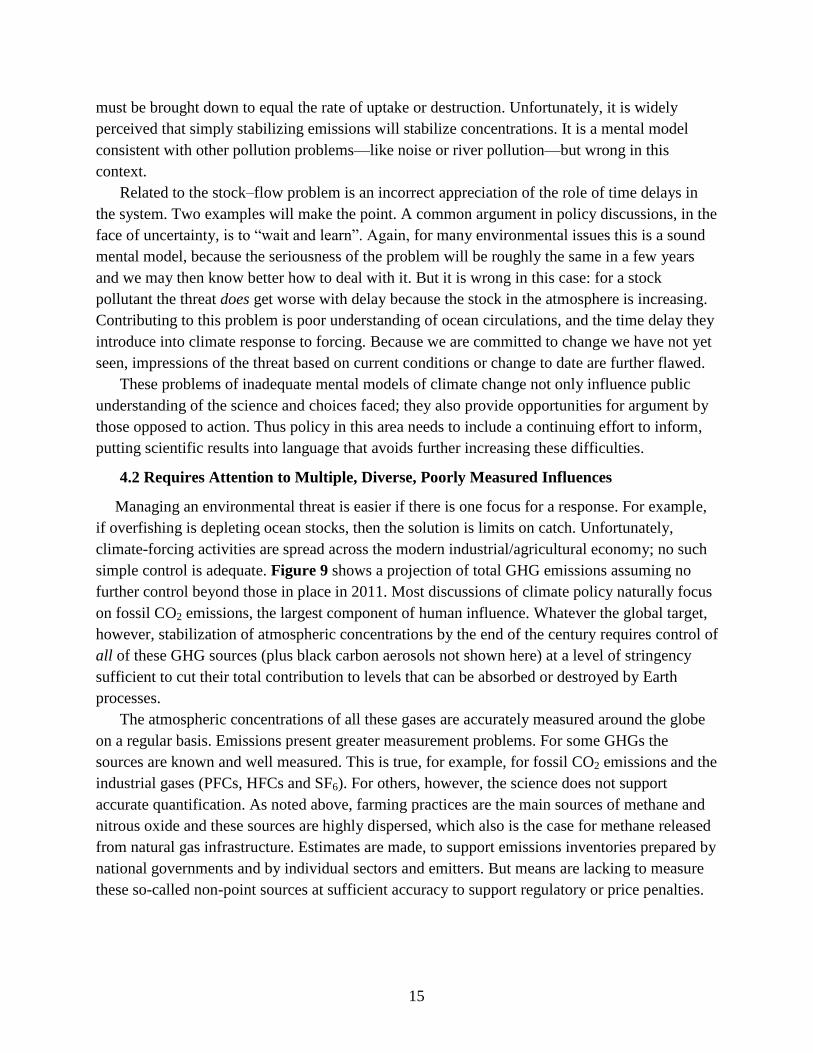
simple control is adequate. Figure 9 shows a projection of total GHG emissions assuming no

further control beyond those in place in 2011. Most discussions of climate policy naturally focus

on fossil CO2 emissions, the largest component of human influence. Whatever the global target,

however, stabilization of atmospheric concentrations by the end of the century requires control of

all of these GHG sources (plus black carbon aerosols not shown here) at a level of stringency

sufficient to cut their total contribution to levels that can be absorbed or destroyed by Earth

processes.

The atmospheric concentrations of all these gases are accurately measured around the globe

on a regular basis. Emissions present greater measurement problems. For some GHGs the

sources are known and well measured. This is true, for example, for fossil CO2 emissions and the

industrial gases (PFCs, HFCs and SF6). For others, however, the science does not support

accurate quantification. As noted above, farming practices are the main sources of methane and

nitrous oxide and these sources are highly dispersed, which also is the case for methane released

from natural gas infrastructure. Estimates are made, to support emissions inventories prepared by

national governments and by individual sectors and emitters. But means are lacking to measure

these so-called non-point sources at sufficient accuracy to support regulatory or price penalties.

16

Figure 9. Global greenhouse gas emissions (MIT JP, 2012).

Similar problems arise in the measurement of emissions from forests destruction, mainly in

the tropics, which is the main component to the land CO2 component in Figure 9. Despite a great

deal of effort to combine on-ground and satellite measurement the irreducible error creates

problems in application to systems of penalty and reward.

A further problem of emissions quantification arises in calculations that appear to be

grounded in the science of climate but that in fact contain elements that lie beyond the domain of

scientific disciplines. In deciding the allocation of mitigation effort there is a need to be able to

express the relative importance of the various GHGs. The mix of these gases varies among

nations, and some weighting scheme is also needed to be able to compute totals for discussion of

equity among parties. Also, such weights are required if there is to be emissions trading among

the gases. The ideal would be a measure of relative future economic and ecological damage

attributable to each, or even a measure of the contribution to future temperature increase. Such

measures raise insurmountable obstacles of uncertainty and estimation, however, so the solution

has been to pick an intermediate level of climate influence: the effect of each on radiative forcing

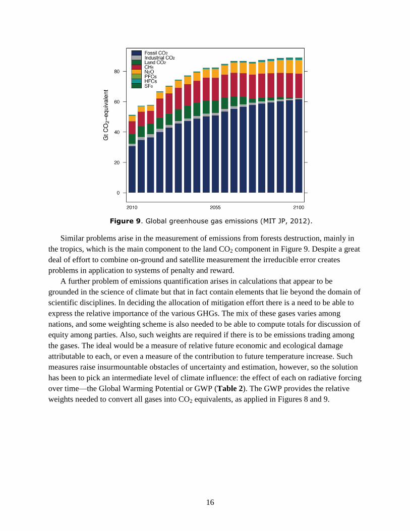
over time—the Global Warming Potential or GWP (Table 2). The GWP provides the relative

weights needed to convert all gases into CO2 equivalents, as applied in Figures 8 and 9.

17

Table 2. Global warming potentials for different integration periods (IPCC, 2007b).

Lifetime

(Years)

Time Horizon (TH) in Years

20 100 500

Methane 12 72 25 7.6

Nitrous Oxide 114 289 298 153

HFC-23 270 12,000 14,800 12,200

HFC-134a 14 3,830 1,430 435

SF6 3,200 16,300 22,800 32,600

The GWPs are calculated by simulating a pulse of each gas in a climate model, tracking the

influence on W/m2

over time, and summing the influences.6 The results then differ by the heat-

trapping power of each substance and the speed by which it is either taken up by the oceans and

terrestrial biosphere or destroyed in the atmosphere. In this calculation there is one key input that

the science cannot resolve: what should be the integration period over which the calculation is

made? A short period gives more weight to shorter-lived gases and vice versa. Table 2 shows the

effect of using a 20, 100 or 500 year period. Through agreements in the IPCC nations have

decided to use the 100-year GWPs for reporting, trading agreements, etc., but much controversy

remains. For example, when there is a focus on climate effects over the next few decades there is

an argument for using the 20-year GWP in order to give a proper weight to methane on this time

horizon. If done the change would triple the weight given a ton of methane in relation to a ton of

CO2. A question also remains whether an additional relative weight should be imposed on

methane for its knock-on effect on the generation of ozone, a greenhouse gas that also damages

CO2-absorbing vegetation.

4.3 Demands Cooperative Effort by Parties with Diverse Interests

Over past decades nations have developed policy regimes to deal with a number of

international environmental problems ranging from the disposal of toxic waste to protection of

endangered species. For some the number of major players was small, simplifying the process of

agreement if interests in the issue were aligned. For example, only a small number of nations are

relevant to agreements to lower stockpiles of nuclear weapons, and in the case of the Montreal

Protocol on Substances that Deplete the Ozone Layer only a few nations were producing the

offending chemicals. For the climate issue the commons problem is truly global. Though not all

nations are essential to reducing the risk, a large number are. Moreover their interests lack

alignment in crucial dimensions.

The nature of this aspect of the challenge can be seen in Figure 10, a projection to 2050 of

energy use (the main source of GHG emissions) assuming no mitigation efforts beyond those in

6 The lifetimes in Table 2 do not indicate when the pulse has completely disappeared from the atmosphere but when

the number of molecules is reduced by 1/e where e=2.72.

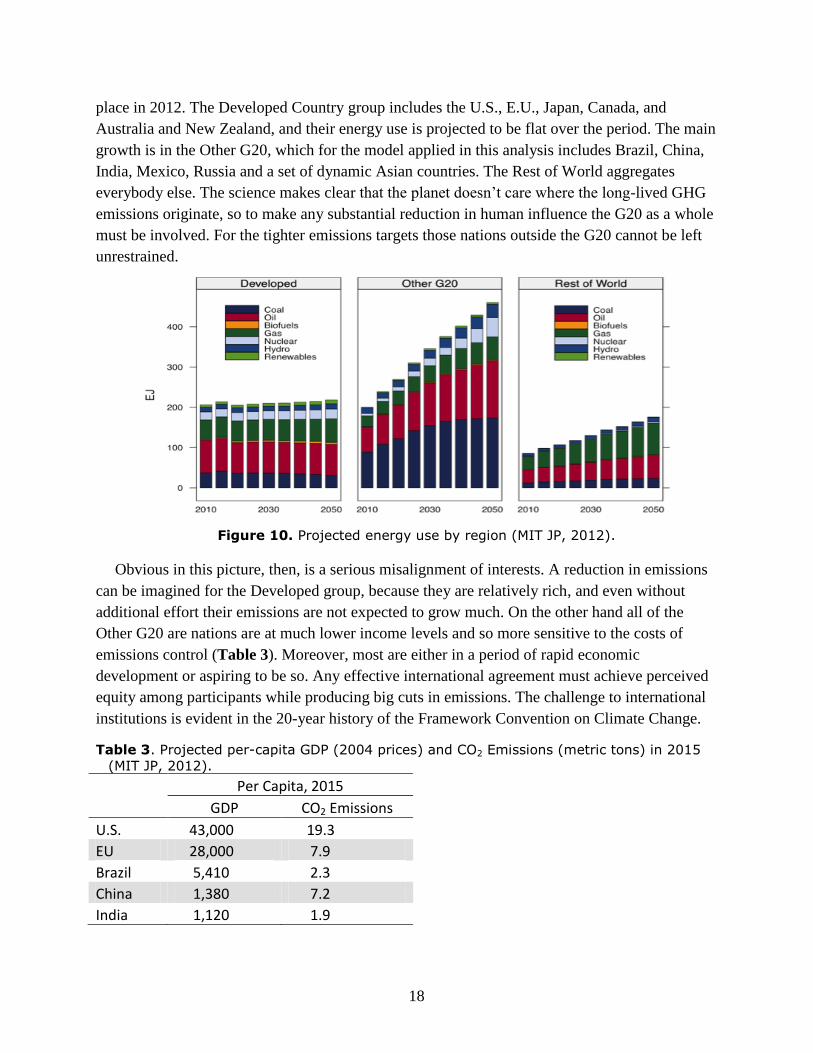
18

place in 2012. The Developed Country group includes the U.S., E.U., Japan, Canada, and

Australia and New Zealand, and their energy use is projected to be flat over the period. The main

growth is in the Other G20, which for the model applied in this analysis includes Brazil, China,

India, Mexico, Russia and a set of dynamic Asian countries. The Rest of World aggregates

everybody else. The science makes clear that the planet doesn’t care where the long-lived GHG

emissions originate, so to make any substantial reduction in human influence the G20 as a whole

must be involved. For the tighter emissions targets those nations outside the G20 cannot be left

unrestrained.

Figure 10. Projected energy use by region (MIT JP, 2012).

Obvious in this picture, then, is a serious misalignment of interests. A reduction in emissions

can be imagined for the Developed group, because they are relatively rich, and even without

additional effort their emissions are not expected to grow much. On the other hand all of the

Other G20 are nations are at much lower income levels and so more sensitive to the costs of

emissions control (Table 3). Moreover, most are either in a period of rapid economic

development or aspiring to be so. Any effective international agreement must achieve perceived

equity among participants while producing big cuts in emissions. The challenge to international

institutions is evident in the 20-year history of the Framework Convention on Climate Change.

Table 3. Projected per-capita GDP (2004 prices) and CO2 Emissions (metric tons) in 2015

(MIT JP, 2012).

Per Capita, 2015

GDP CO2 Emissions

U.S. 43,000 19.3

EU 28,000 7.9

Brazil 5,410 2.3

China 1,380 7.2

India 1,120 1.9

19

4.4 Reveals Uncertainty that Complicates Mitigation Decision

As noted above, each member of a large family of climate models projects change over this

century and beyond, but they differ in important details of future patterns of temperature and

precipitation. Moreover, uncertainty analysis using a single model (Figure 8) reveals great

uncertainty even if emissions uncertainty is removed (as in the right-hand wheel in the figure).

These results reflect the current state of the science as employed in projections of the behavior of

the climate system in response to human influence. Nevertheless, they clearly suggest serious

future risk to ecosystems and national economies.

Unfortunately, this unavoidable level of uncertainty also impedes the formulation of

commitment to reduce the risk. Some participants in the policy process simply don’t trust the

science. And even those with respect for the science may interpret the uncertainty to mean that

understanding is yet insufficient to justify action to limit emissions. At worst, the issue is cast as

a matter of “belief”. In this formulation climate change is either real or it is not, like the virgin

birth, and uncertainty in scientific analyses is taken as indicating a lack of proof. Proper

application of the science will cast the climate threat not as a true-false question (act urgently if it

is real; do nothing if it is not) but as a challenge of risk management. This is a way of thinking

about decision under uncertainty that we apply all the time in our private lives (e.g., how

radically to change diet to lower cholesterol and the risk of heart disease) and in public decision

(how aggressively to pursue a vaccination program to manage the risk of flu epidemic). The

debate of climate policy has been too often driven away from this way of formulating the choice,

however, and correction of this misdefinition would go a long way toward overcoming the

barriers created by unavoidable uncertainty about the magnitude of the threat.

Even given acceptance of climate change as a serious risk, limits to our understanding also

lead to difficulties in deciding the proper response. This is in part because the science cannot yet

support precise quantitative descriptions of what the uncertainties actually are—a shortcoming

has come to be known as the problem of “fat tails”. To frame the issue, consider the following

question: What should be the CO2 price in the European Trading System? Most observers would

agree that the price at the time of this writing (around €7 per ton CO2) is too low, but also that

€150 would be too high. Where do these views come from? Apart from notions of political

feasibility, which no doubt intervene, a substantial influence is a concept in economics that the

policy task is to appropriately spread pain over time. Emissions now will cause damage in the

future (say, in lost consumption), and we can lower future pain by taking some penalty now

(diverting current consumption to emissions mitigation). Impressions of future economic and

environmental damage may be foggy, and the way future and current costs are compared may be

obscure, but the underlying conception is nonetheless common, and not just among economists.

It leads to opinions about the price today and to the expectation that it should rise over time as

future emissions are expected to cause larger incremental damage.

This benefit-cost way of thinking about mitigation effort is implemented in policy procedures.

For example, for federal rulemakings and other policy decisions the U.S. Office of Management

and Budget requires an analysis of monetary costs and benefits. To this end the U.S.

20

Environmental Protection Agency must prepare an analysis of the monetary benefit of reducing a

current ton of CO2—what is called the Social Cost of Carbon (SCC)—to be compared with the

cost of measures to limit emissions (US EPA, 2010). The estimation of the SCC is based on a set

of computer models that simulate the temperature effect of an additional ton of CO2 today,

impose a mathematical function to represent estimated damage of that change in the future, and

(employing some discount rate) smooth the pain over time in a way that maximizes some

measure of human welfare.7

The same formulation is applied when the analysis includes formal representations of

uncertainty in these processes. To highlight difficulties of the climate issue, consider the simpler

case of river pollution by urban waste. For a given waste discharge there is uncertainty in the

resulting water quality—because of uncertainty in flow, temperature, biological processes, etc.

And whatever the water quality in the river there is uncertainty in the damage, say in fish kills

and human disease. To calculate the benefit of reducing urban discharge the range of potential

water quality outcomes can be weighted by their probabilities to compute an expected quality

level. And potential but uncertain levels of damage, for that expected river quality, can be

weighted by their probabilities to yield an overall estimate of the expected benefit of a reduction

in discharge.8 For water pollution this is a credible and easily understood calculation because we

have extensive experience with the biology of rivers and with the effects of polluted waters on

fish and human health.

Now consider the difference with anthropogenic climate change. We have just one planet, and

human greenhouse emissions are pushing some of its climate processes outside the experience of

the past 20,000 years (see Figure 6) and longer. This means that estimates of the parameters of

uncertainty measures of climate response are themselves uncertain. (Various names are given to

this condition including deep uncertainty and structural uncertainty).

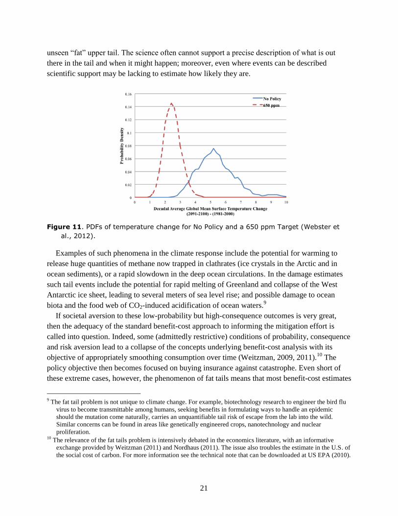
As an example, look again wheel in Figure 8b, where policy constraint removes the

uncertainty in emissions. Underlying the uncertainty in that projection are estimates, based

heavily on analysis of climate behavior in the 20th

century, of the parameters (e.g., mean,

variance) of probability distributions of cloud behavior and aerosol effects (Figure 3), deep ocean

circulations (Figure 4), and aspects of CO2 emissions from the terrestrial biosphere (Figure 2).

The resulting probability distribution that was restated in the form of the Figure 8 roulette wheel

is shown in Figure 11. The distribution for the policy (650 ppm) case looks like a bell-shaped

curve (a normal distribution) whose tails are pretty “thin”: under the 650 ppm target the

probability of a temperature increase exceeding 4°C is near zero. However, given that the

uncertainty parameters are based on a single planet, with limited data about this one, these

parameters are themselves uncertain. So, if we could take this parameter uncertainty into account

the resulting distribution would be more spread out. To use the term introduced earlier, it has an

7 There are, of course, many difficulties with such analyses, not least being the valuation of non-market effects and

the choice of discount rate, but here the focus is on issues in the underlying climate science. 8 To see this done for climate using an integrated assessment model see Nordhaus, 2008.

21

unseen “fat” upper tail. The science often cannot support a precise description of what is out

there in the tail and when it might happen; moreover, even where events can be described

scientific support may be lacking to estimate how likely they are.

Figure 11. PDFs of temperature change for No Policy and a 650 ppm Target (Webster et

al., 2012).

Examples of such phenomena in the climate response include the potential for warming to

release huge quantities of methane now trapped in clathrates (ice crystals in the Arctic and in

ocean sediments), or a rapid slowdown in the deep ocean circulations. In the damage estimates

such tail events include the potential for rapid melting of Greenland and collapse of the West

Antarctic ice sheet, leading to several meters of sea level rise; and possible damage to ocean

biota and the food web of CO2-induced acidification of ocean waters.9

If societal aversion to these low-probability but high-consequence outcomes is very great,

then the adequacy of the standard benefit-cost approach to informing the mitigation effort is

called into question. Indeed, some (admittedly restrictive) conditions of probability, consequence

and risk aversion lead to a collapse of the concepts underlying benefit-cost analysis with its

objective of appropriately smoothing consumption over time (Weitzman, 2009, 2011).10

The

policy objective then becomes focused on buying insurance against catastrophe. Even short of

these extreme cases, however, the phenomenon of fat tails means that most benefit-cost estimates

9 The fat tail problem is not unique to climate change. For example, biotechnology research to engineer the bird flu

virus to become transmittable among humans, seeking benefits in formulating ways to handle an epidemic

should the mutation come naturally, carries an unquantifiable tail risk of escape from the lab into the wild.

Similar concerns can be found in areas like genetically engineered crops, nanotechnology and nuclear

proliferation. 10

The relevance of the fat tails problem is intensively debated in the economics literature, with an informative

exchange provided by Weitzman (2011) and Nordhaus (2011). The issue also troubles the estimate in the U.S. of

the social cost of carbon. For more information see the technical note that can be downloaded at US EPA (2010).

22

of mitigation effort—valuable as they are in tuning intuition—do not convey the whole story.

Aversion to risks that the science cannot yet quantify will be an important influence on policy

deliberations, leaning toward a more aggressive current response than the standard benefit-cost

analysis would indicate, and to support for those who would inject the precautionary principle

into policy debates.

This state of scientific understanding of the climate system calls for the use of policy

instruments that can be flexible over time as earth-system knowledge is gained. (The same

conclusion emerges from consideration of uncertainty in the costs of control. and this concern

arises in decisions about adaptation as well as for mitigation.) As in most problems of risk

management under uncertainty, climate policy is best thought of as facilitating a process of

sequential decision: act now based on current knowledge, learn over time, and revise later based

on any new information. It is a model of the policy process that is consistent with the fact that

governments cannot make commitments for long periods of time, but its implications are not

always considered in formulating the details of mitigation proposals.

4.5 Creates Special Difficulty in Formulating Adaptation Measures

Whatever success we may have in limiting greenhouse emissions the Planet faces changes in

climate to which human and natural systems will have to adapt. Many of these adjustments will

take place gradually, in response to change as experienced year to year, “on the ground” as it

were. For example, shifts in rainfall and temperature will change the economics of different

crops and where they are grown, leading to shifts over time; changes in atmospheric conditions

and availability of food supplies will lead to changes in migration patterns of birds, other animals

and insects. Indeed some of these effects are seen in the response of natural systems to the

climate change already experienced.

However, some adaptation could be very expensive if it is not possible to anticipate what is

coming. For example, large capital facilities underlie the water management systems that support

irrigated agriculture and industrial and residential water services. These systems take a long time

to develop and are very costly, so systems built now need to take account of conditions under

projected climate change, and appropriate near-term revision of existing systems could lower the

economic loss when the climate change comes. For instance, a change in mountain runoff from

slowly melting snow to winter and spring rainfall may call for substantial revision in the design

of irrigation systems and the water storage reservoirs that support them. Without a change in

technology electric powerplants may not be able to depend on streams and rivers for the quantity

and temperature of flow needed for cooling.

Or, to take a regulatory example, many governments compute maps of likely flooding from

rivers and streams and use this information in determining zoning regulations, requirements for

the design of structures’ flood zones, and insurance rates. These estimates determine the location

of large swathes of urban and industrial activity and thus the risks to which they will be subject

in the future. Many governments and private industries are already trying to formulate

23

investment and regulatory policies that anticipate potential change in the hope of lowering the

associated economic cost and social disruption.

But here again the climate science intercedes. The uncertainty in future change at global scale

is already great, as indicated in Figure 8. But adaptation decisions depend on climate conditions

at local scale: the particular agricultural zone, valley or river basin. At these local scales the

uncertainty in future change is even greater. Even computer models of the climate that agree on

change at global scale may yield estimates of the change in runoff in a particular river basin that

differ not only in magnitude but also in sign: some project more water, some less. Indeed it is a

general characteristic Earth systems that the smaller the region of interest the greater the

additional uncertainty in modeling the climate change effects. Another pass through the 20th

century (http://www.nasa.gov/topics/earth/features/2011-temps.html) suggests this result should

be no surprise.

The implication of the higher level of uncertainty for policy is that the planning of

anticipatory adaptation, be it by investment or regulatory change, needs to be based on an

expression of the full uncertainty of future projections at local scale. Decisions made on the basis

of one or two scenarios could lead to costly decisions, and very often the proper response may be

to provide more flexibility for adjusting to future conditions that cannot now be specified even

though there is a high likelihood that some change is coming.

5. COMBINED EFFECTS ON THE CHOICE OF RESPONSE STRATEGY

The formulation of strategy to deal with the climate change threat is greatly complicated by

the combination of these various characteristics of the issue. The magnitude of the climate

challenge can again be highlighted in contrast to a superficially similar problem: formulating a

respond to the threat to the stratospheric ozone layer by a set of industrial gases. In negotiation of

the Montreal Protocol the interest of the main parties (developed countries and firms that

produced these gases) were aligned, a narrow set of gases were at issue, corresponding policy on

adaptation to increased UV radiation was not an issue, and compensation of nations adjusting to

the change was easily handled. It is not so easy with climate, where:

Participation is required by parties whose interests are not aligned;

Emissions with different origins and lifetimes, some poorly measured, must be dealt with;

Adaptation is a serious issue and not completely separate from mitigation;

Uncertainty is greater and harder to quantify; and

Involvement of both rich and poor nations will require substantial financial differences in

effort according to ability and likely some financial assistance.

And, of course these same issues serve to complicate not only international agreement but also

the formulation of the domestic actions within each country.

Given these characteristics of the climate issue, the appropriate strategy for the needed

international response remains unclear even after two decades of struggle. Is it to best to follow

the Montreal Protocol model and seek a global agreement covering all nations and all these

issues? This is the strategy underlying the various stages of negotiation under the Framework

24

Convention on Climate Change, including the latest effort under the Durban Platform (UN

FCCC, 2011). Is it likely more productive to focus on various “club” agreements, which may be

built around groups where interests are more closely aligned (e.g., the Asia-Pacific Partnership,

Major Economies Forum, G-20, G8+5)? Or is a set of bilateral agreements among major players

the way forward?

There is even a choice of which of the human influences should be the focus in any

agreement. Negotiations in the Framework Convention have taken (on all at once) long-lived and

short-lived gases weighted by the Global Warming Potentials in Table 2. An alternative

suggested by UNEP and WMO (2011) is to seek an agreement focused on short-lived

substances—methane, and black carbon—motivated in part that agreement may be facilitated by

the non-climate co-benefits that would result from the reduction in air pollution. Or is it likely

that this combination of problem characteristics will necessarily lead to a combination of all, in a

loosely coordinated regime “complex” (Keohane and Victor, 2010)?11

Though one can hope

national interests may come to be better aligned, the scientific characteristics of the climate

threat are not likely to change in coming decades, so the complications it introduces will

continue.

Acknowledgments

This paper was produced originally for the Global Governance Programme of the Robert

Schulman Centre for Advanced Studies, European University Institute, Florence, and released as

EUI Working Paper RSCAS 2012/72.

6. REFERENCES

Cole, D., 2011: From Global to Polycentric Climate Governance. EUI Working Paper RSCAS

2011/30, Robert Schuman Centre for Advanced Studies, European University Institute,

Florence.

IPCC [Intergovernmental Panel on Climate Change], 2007a: Synthesis Report, Summary for

Policymakers. R. Pachauri and A. Reisinger (eds.), Cambridge University Press: Cambridge,

United Kingdom and New York, NY

(http://www.ipcc.ch/publications_and_data/ar4/syr/en/spm.html).

IPCC [Intergovernmental Panel on Climate Change], 2007b: Climate Change 2007: The

Physical Science Basis. Contribution of Working Group I to the Fourth Assessment Report of

the Intergovernmental Panel on Climate Change. S. Solomon, D. Qin, M. Manning, Z. Chen,

M. Marquis, K.B. Avery, M. Tignor and H.L. Miller (eds.), Cambridge University Press:

Cambridge, United Kingdom and New York, NY.

Keohane, R., and D. Victor, 2010: The Regime Complex for Climate Change, Discussion Paper

10-33, Harvard Project on International Agreements, Kennedy School of Government, Harvard

University, Cambridge, MA.

Kahneman, D., 2011: Thinking Fast and Slow, Farrar, Straus and Giroux: New York, NY.

11

Expectation of this outcome is consistent with a more formal analysis of “polycentric” governance as applied to

climate change by Cole (2011).

25

Kiehl, J. and K. Trenberth, 1979: Earth’s Annual Global Mean Energy Budget. Bull. Amer.

Meteor. Soc., 78: 197–208.

MIT JP [MIT Joint Program on the Science and Policy of Global Change], 2012: Energy and

Climate Outlook 2012. Cambridge, MA.

(http://globalchange.mit.edu/research/publications/other/special/2012Outlook).

NSIDC [National Snow and Ice Date Center], 2012: Press Release: Arctic sea ice shatters

previous low records; Antarctic sea ice edges to record high. Boulder, CO

(http://nsidc.org/news/press/20121002_MinimumPR.html).

Nordhaus, W., 2008: A Question of Balance: Weighing the Options on Global Warming Policies.

(available for download at http://nordhaus.econ.yale.edu/cv_current.htm).

Nordhaus, W., 2011: The Economics of Tail Event with an Application to Climate Change.

Review of Environmental Economics and Policy, 5(2): 240–257.

Sokolov, A., P. Stone, C. Forest, R. Prinn, M. Sarofim, M. Webster, S. Paltsev, C.A. Schlosser,

D. Kicklighter, S. Dutkiewicz, J. Reilly, C. Wang, B. Felzer, J. Melillo and H. Jacoby, 2009:

Probabilistic Forecast for 21st Century Climate Based on Uncertainties in Emissions (without

Policy) and Climate Parameters. Journal of Climate, 22(19): 5175–5204 [Erratum].

Sterman, J., 2011: Communicating climate change risks in a skeptical world. Climatic Change,

108: 811–826.

UNEP and WMO [UN Environment Program and World Meteorological Organization], 2011:

Integrated Assessment of Black Carbon and Tropospheric Ozone. United Nations Environment

Program and World Meteorological Organization, UNEP/GC/26/INF/20.

UN FCCC [UN Framework Convention on Climate Change], 2011: Establishment of and Ad

Hoc Working Group on the Durban Platform for Enhanced Action. Conference of the Parties,

Seventeenth Session, FCCC/CP/2011/L.10.

US EPA [US Environmental Protection Agency], 2010: The Social Cost of Carbon: Estimating

the Benefits of Reducing Greenhouse Gas Emissions.

(http://www.epa.gov/climatechange/EPAactivities/economics/scc.html).

US NAS [US National Academy of Sciences], 1979: Carbon Dioxide and Climate: A Scientific

Assessment, Washington, D.C.

US NASA [US National Atmospheric and Space Administration], 2004: NASA Science Space

News, Washington, D.C. (http://science.nasa.gov/science-news/science-at-

nasa/2004/05mar_arctic/).

US NOAA [US National Oceanic and Atmospheric Administration, National Climate Data

Center], 2012: State of the Climate: Global Analysis for August 2012, published online

September 2012, retrieved on October 1, 2012 (http://www.ncdc.noaa.gov/sotc/global/2012/8).

Webster, M., A. Sokolov, J. Reilly, C. Forest, S. Paltsev, C.A. Schlosser, C. Wang, D.

Kicklighter, M. Sarofim, J. Melillo, R. Prinn and H. Jacoby, 2012: Analysis of policy targets

under uncertainty. Climatic Change, 112(3-4): 569–583.

Weitzman, M., 2009: On Modeling and Interpreting the Economics of Catastrophic Climate

Change. Review of Economics and Statistics, 91(1): 1–19.

Weitzman, M., 2011: Fat-Tailed Uncertainty in the Economics of Climate Change. Review of

Environmental Economics and Policy. 5(2): 275–292.

CLIMATE POLICY NOTE SERIES of the MIT Joint Program on the Science and Policy of Global Change

Contact the Joint Program Office to request a copy. The Climate Policy Note Series is distributed at no charge.

FOR THE COMPLETE LIST OF JOINT PROGRAM CLIMATE POLICY NOTES: http://globalchange.mit.edu/research/publica-tions/other/climatepolicy

2. Implications of Climate Science for Policy Jacoby July 2013

1. Climate Change Today Prinn et al. April 2011