Prepared for submission to JHEP

Importance and construction of features in identifying

new physics signals with deep learning

Chang-Wei Loh,a Rui Zhang,a Yong-Heng Xu,a Zhi-Qiang Qian,a Si-Cheng Chen,b

He-Yang Long,a You-Hang Liu,a De-Wen Cao,a Wei Wanga and Ming Qia,1

aNanjing University, 22 Hankou Road, Nanjing, Jiangsu, ChinabNanjing University of Aeronautics and Astronautics, 29 Jiangjun Dadao, Nanjing, Jiangsu, China

E-mail: qming@nju.edu.cn

Abstract: Advances in machine learning have led to an emergence of new paradigms in

the analysis of large data which could assist traditional approaches in the search for new

physics amongst the immense Standard Model backgrounds at the Large Hadron Collider.

Deep learning is one such paradigm. In this work, we first study feature importance ranking

of signal-background classification features with deep learning for two Beyond Standard

Model benchmark cases: a multi-Higgs and a supersymmetry scenario. We find that the

discovery reach for the multi-Higgs scenario could still increase with additional features.

In addition, we also present a deep learning-based approach to construct new features to

separate signals from backgrounds using the ATLAS detector as a specific example. We

show that the constructed feature is more effective in signal-background separation than

commonly used features, and thus is better for physics searches in the detector. As a

side application, the constructed feature may be used to identify any momentum bias in

a detector. We also utilize a convolutional neural network as part of the momentum bias

checking approach.

Keywords: deep learning, classification feature, LHCarX

iv:1

712.

0380

6v1

[he

p-ex

] 1

1 D

ec 2

017

Contents

1 Introduction 1

2 Feature Importance in Beyond Standard Model Signals 3

2.1 Multi-Higgs Signal 3

2.2 Supersymmetry Signal 7

3 Constructing Features with Deep Learning 10

4 Summary 14

1 Introduction

After the discovery of a light Higgs boson [1, 2], there is a general expectation for particles

from physics beyond the Standard Model (BSM) to be observed in the ATLAS and CMS

detectors at the Large Hadron Collider (LHC). However, none has been found so far.

Often, to discriminate signals originating from new physics against the immense Standard

Model (SM) backgrounds, various signal-background classification features, including raw

kinematic features of final states physics objects as measured by the detector and derived

features which can be computed from the combinations of these raw features, are used.

Typical raw features include the transverse momentum pT and pseudorapidity η of the final

states physics objects and missing energy MET of the physics events, while derived features

are commonly physics inspired which includes the invariant masses of a set of physics

objects. The choice of using any features lies in whether the classification performance and

hence the discovery significance could be improved with the inclusion of a feature as part

of the physics event selection cuts.

Employing machine learning in signal-background classification problems in particle

physics is not new. In fact, machine learning approaches typically outperform the tradi-

tional linear cuts used for event selections, as the latter could not capture the non-linear

correlations among the classification features. For instance, in the search for new physics in

the WWbb channel with the ATLAS detector, which assumed a multi-Higgs boson cascade

decay [3] as a benchmark process, a machine learning tool, i.e. boosted decision tree (BDT)

[4] signal-background classifier has been used. In the continuous attempt to gain an edge

in discovering new physics, a new machine learning paradigm, known as deep learning [5]

has recently caught the attention of the particle physics community.

Deep learning is a class of machine learning which has had ubiquitous success in a

plethora of disparate fields, ranging from arts [6] and language [7] to genetics [8] and drug

discovery [9]. In high-energy physics, various studies have been done for its potential use in

particle collisions [10], exotics searches [11], jet classifications [12–14] and the monitoring

– 1 –

of superconducting magnets at the LHC [15]. Deep learning can be regarded as an ex-

tension of the artificial neural network, but with more hidden layers and more versatile in

terms of the connection between neurons in the layers. The versatility of the connections

enables the emergence of new network architectures such as the autoencoder [16], convo-

lutional neural network [17], long short-term memory [18] and recursive neural network

[19]. Succinctly, deep neural networks (DNN) is a highly effective data-driven function

approximator that seeks to model the quantity of interest y using data from a vector of

inputs x with DL(x, p) = y, where p are parameters of the DNN; their values are found

during the training stage of the network. In the case of a signal-background classification

problem, x would be the classification features and y would be the event class, i.e. a signal

or a background. DNN is appealing as it bypasses the need for assumptions about the

underlying mechanisms that produce the data, and instead, assist us in gaining insights as

to the mechanisms that produce them.

In many areas, it is true that machines outperform humans on problems tailored to

achieve a certain aim. Machines optimizes their inputs with one aim in mind, i.e. to achieve

the best possible target pertaining to that aim. In particle physics, given kinematic inputs

from the detectors, we construct detector-agnostic features with physics interpretation

that may or may not work optimally for signal-background separations in an experimental

setting. This contradicts the aim of optimizing a signal-background separation. To search

for some new unknown physics, one desires to achieve the best possible discovery reach given

the amount of data collected at the LHC. Could machine learning assist in constructing

new features to achieve this aim optimally?

Common to all machine learning endeavors in physics event selection cuts, is the search

for new classification features as inputs to the machine learning classifiers. For instance,

in supersymmetry (SUSY) searches, much work has been done to craft new classification

features [20–23] to assist in increasing the signal-background discrimination power. How-

ever, an increase in the number of features used in machine learning approaches would

evoke a high computational cost in doing a single event class prediction and the curse of

dimensionality; the latter refers to the decrease in the accuracy of a classifier prediction

with increasing number of input features when the data is sparse in addition to the larger

uncertainty in the prediction.

Therefore, in this work, we first compare deep learning with BDT, where the latter is a

commonly used machine learning approach in particle physics, in their effectiveness on new

physics searches. We also perform a feature importance ranking with respect to the machine

learning methods to identify the subset of features that gives an optimal classification. We

demonstrate this using two benchmark processes: multi-Higgs, which is also of relevance

to models with an extended Higgs sector [24], and SUSY. The datasets used here has been

used previously in [11]. We then present an approach based on deep learning to construct

new features from some raw kinematic features obtained from a simulation of the ATLAS

detector using the Higgs(Z boson) decaying to two tau leptons as the signal(background)

class, where both decays have already been observed at the LHC [25, 26]. Using such

already known signals and backgrounds would provide a good testing ground at the LHC

for the deep learning-based approach. We also discuss some implications of the constructed

– 2 –

features, in particular as a momentum bias checking tool.

2 Feature Importance in Beyond Standard Model Signals

2.1 Multi-Higgs Signal

In the multiple Higgs bosons scenario, the model contains a heavy neutral Higgs H (425

GeV), an intermediate charged Higgs H± (325 GeV) and a light Higgs boson h (125 GeV).

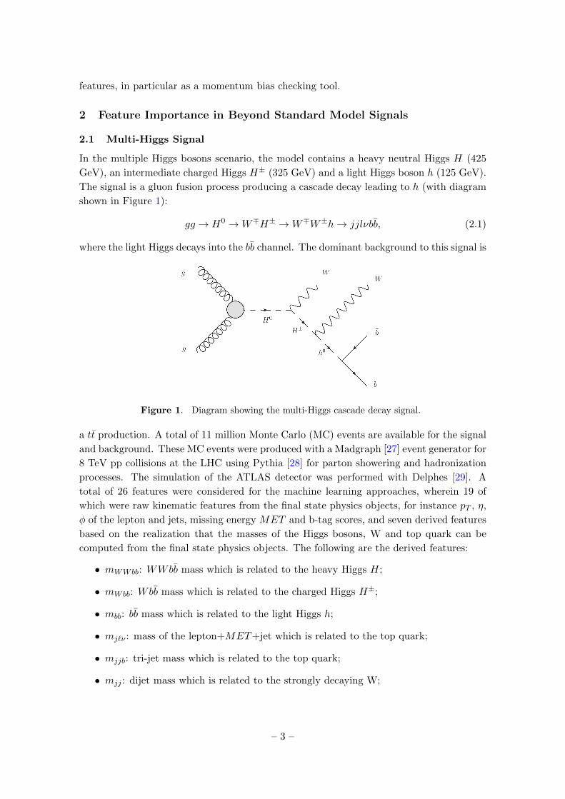
The signal is a gluon fusion process producing a cascade decay leading to h (with diagram

shown in Figure 1):

gg → H0 →W∓H± →W∓W±h→ jjlνbb̄, (2.1)

where the light Higgs decays into the bb̄ channel. The dominant background to this signal is

Figure 1. Diagram showing the multi-Higgs cascade decay signal.

a tt̄ production. A total of 11 million Monte Carlo (MC) events are available for the signal

and background. These MC events were produced with a Madgraph [27] event generator for

8 TeV pp collisions at the LHC using Pythia [28] for parton showering and hadronization

processes. The simulation of the ATLAS detector was performed with Delphes [29]. A

total of 26 features were considered for the machine learning approaches, wherein 19 of

which were raw kinematic features from the final state physics objects, for instance pT , η,

φ of the lepton and jets, missing energy MET and b-tag scores, and seven derived features

based on the realization that the masses of the Higgs bosons, W and top quark can be

computed from the final state physics objects. The following are the derived features:

• mWWbb: WWbb̄ mass which is related to the heavy Higgs H;

• mWbb: Wbb̄ mass which is related to the charged Higgs H±;

• mbb: bb̄ mass which is related to the light Higgs h;

• mj`ν : mass of the lepton+MET+jet which is related to the top quark;

• mjjb: tri-jet mass which is related to the top quark;

• mjj : dijet mass which is related to the strongly decaying W;

– 3 –

Figure 2. Feature importance ranking shown as the AUC vs. number of features k using DNN

and BDT. For each k-th data point, we also indicate the k-th important feature F ∗k used to form

the optimal feature set {F ∗k , ..., F

∗2 , F

∗1 } to obtain the corresponding AUC.

• m`ν : mass of the lepton+MET which is related to the weakly decaying W.

For ensuring the efficient training of the machine learning approaches, the MC data

was preprocessed in order to standardize the features to some common range of values.

This was done by scaling the features, i.e. dividing each feature by its maximum value

within the dataset used. To measure the classification performance of machine learning

approaches as well as simultaneously perform a feature importance ranking for the 26

features, we plotted the AUC, i.e. the area under the receiver operating characteristic

curve (ROC) vs. the number of features k used to obtain the AUC result (see Figure 2).

In brief, an ROC is a plot of the signal efficiency vs. background rejection. An AUC of 0.5

indicates random classification, while an AUC of 1 corresponds to a perfect classification.

In Figure 2, we show the classification performance and feature importance ranking for a

deep learning and BDT classifier. For each k-th point in Figure 2, we indicate the k-th

most important feature which was added to the subset of important features to obtain the

AUC. For the BDT, the optimal set of k was found through a permutation of the values

of each feature [30]. For deep learning, we designed a DNN architecture with a bottleneck

neuron (see Figure 3) that was trained to minimize the cross-entropy loss function with a

softmax activation function at the output layer. To identify the first important feature out

of the 26 features using the DNN with a bottleneck neuron, 26 input neurons representing

the 26 features are forced to pass through the bottleneck neuron before connecting to the

first fully-connected layer of the DNN during the training stage. Once the training ends,

the weight of each input neuron at the bottleneck is extracted. The feature with the largest

weight is regarded as the first important feature. Subsequently, in order to identify the

second most important feature out of the remaining 25 features, a total of 25 input neurons

representing the remaining 25 features are forced to pass through the bottleneck neuron

before connecting to the first fully-connected layer, while the input neuron corresponding

– 4 –

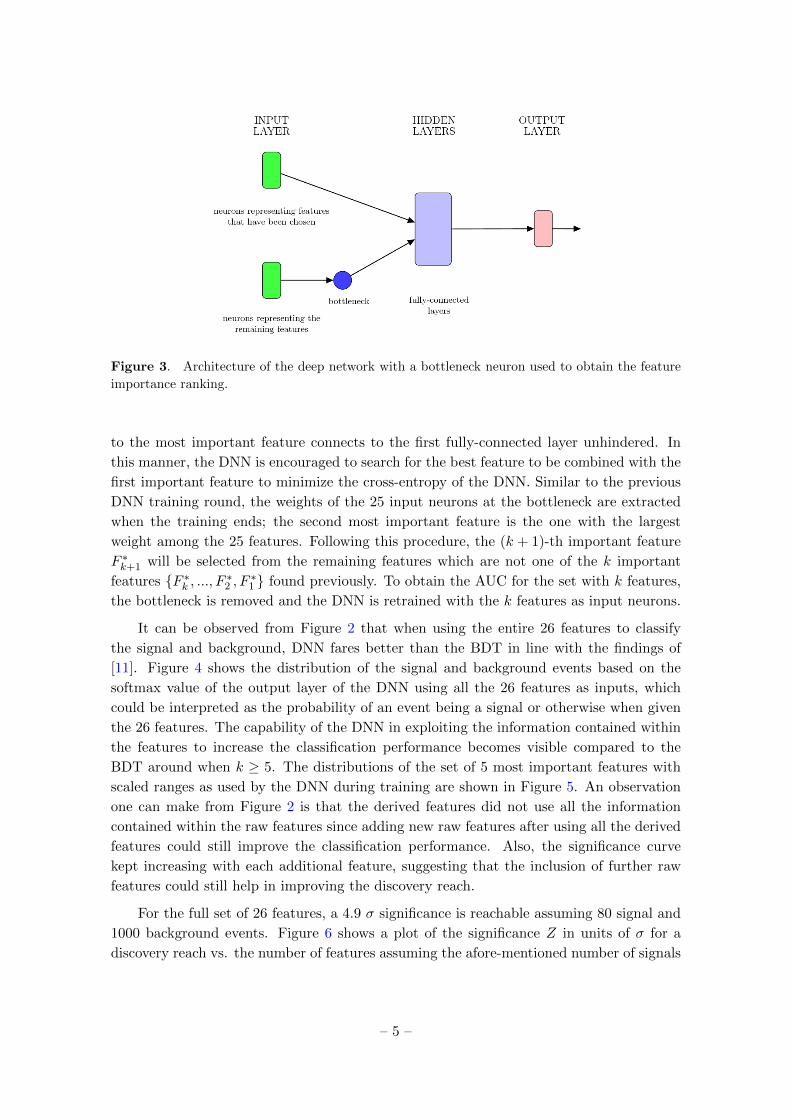
Figure 3. Architecture of the deep network with a bottleneck neuron used to obtain the feature

importance ranking.

to the most important feature connects to the first fully-connected layer unhindered. In

this manner, the DNN is encouraged to search for the best feature to be combined with the

first important feature to minimize the cross-entropy of the DNN. Similar to the previous

DNN training round, the weights of the 25 input neurons at the bottleneck are extracted

when the training ends; the second most important feature is the one with the largest

weight among the 25 features. Following this procedure, the (k + 1)-th important feature

F ∗k+1 will be selected from the remaining features which are not one of the k important

features {F ∗k , ..., F

∗2 , F

∗1 } found previously. To obtain the AUC for the set with k features,

the bottleneck is removed and the DNN is retrained with the k features as input neurons.

It can be observed from Figure 2 that when using the entire 26 features to classify

the signal and background, DNN fares better than the BDT in line with the findings of

[11]. Figure 4 shows the distribution of the signal and background events based on the

softmax value of the output layer of the DNN using all the 26 features as inputs, which

could be interpreted as the probability of an event being a signal or otherwise when given

the 26 features. The capability of the DNN in exploiting the information contained within

the features to increase the classification performance becomes visible compared to the

BDT around when k ≥ 5. The distributions of the set of 5 most important features with

scaled ranges as used by the DNN during training are shown in Figure 5. An observation

one can make from Figure 2 is that the derived features did not use all the information

contained within the raw features since adding new raw features after using all the derived

features could still improve the classification performance. Also, the significance curve

kept increasing with each additional feature, suggesting that the inclusion of further raw

features could still help in improving the discovery reach.

For the full set of 26 features, a 4.9 σ significance is reachable assuming 80 signal and

1000 background events. Figure 6 shows a plot of the significance Z in units of σ for a

discovery reach vs. the number of features assuming the afore-mentioned number of signals

– 5 –

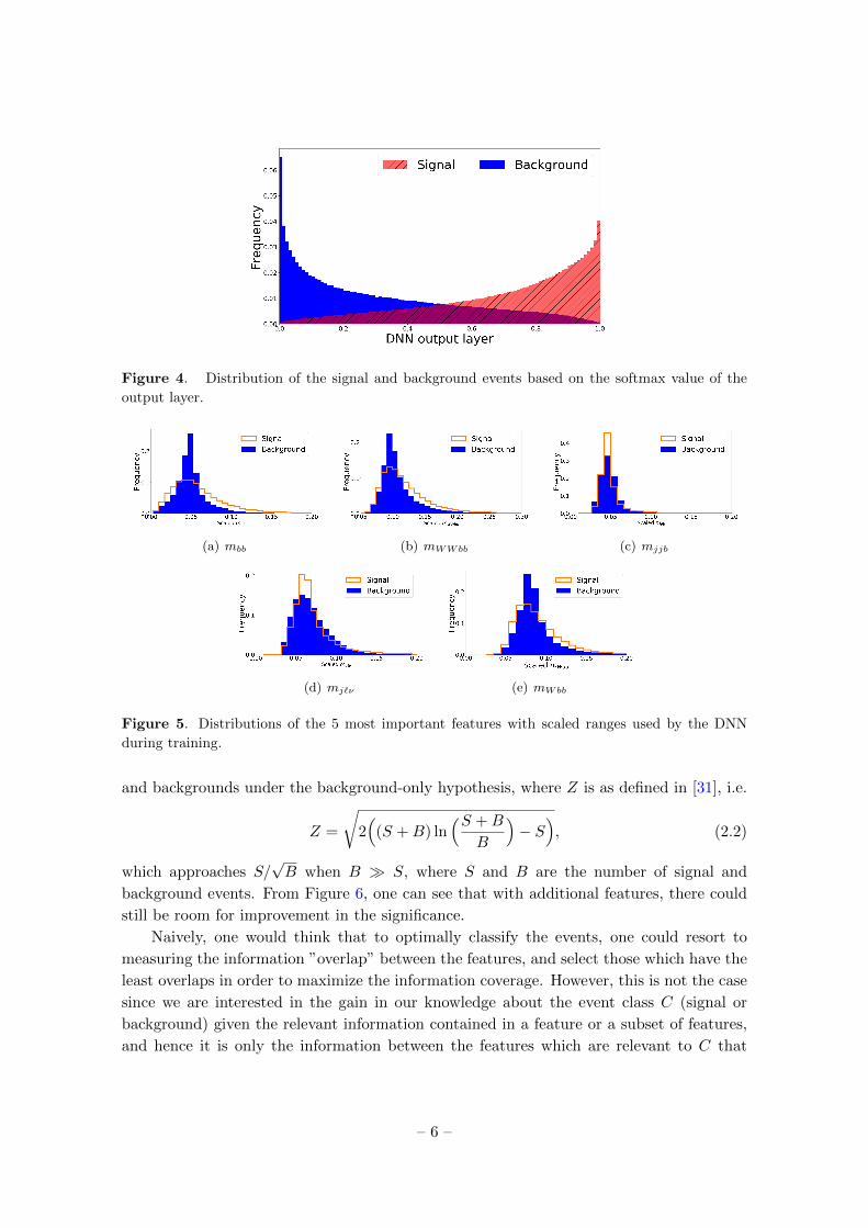
Figure 4. Distribution of the signal and background events based on the softmax value of the

output layer.

(a) mbb (b) mWWbb (c) mjjb

(d) mj`ν (e) mWbb

Figure 5. Distributions of the 5 most important features with scaled ranges used by the DNN

during training.

and backgrounds under the background-only hypothesis, where Z is as defined in [31], i.e.

Z =

√2(

(S +B) ln(S +B

B

)− S

), (2.2)

which approaches S/√B when B � S, where S and B are the number of signal and

background events. From Figure 6, one can see that with additional features, there could

still be room for improvement in the significance.

Naively, one would think that to optimally classify the events, one could resort to

measuring the information ”overlap” between the features, and select those which have the

least overlaps in order to maximize the information coverage. However, this is not the case

since we are interested in the gain in our knowledge about the event class C (signal or

background) given the relevant information contained in a feature or a subset of features,

and hence it is only the information between the features which are relevant to C that

– 6 –

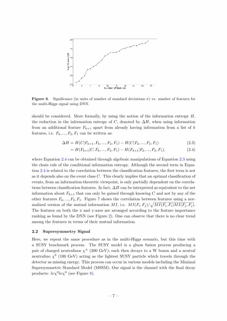
Figure 6. Significance (in units of number of standard deviations σ) vs. number of features for

the multi-Higgs signal using DNN.

should be considered. More formally, by using the notion of the information entropy H,

the reduction in the information entropy of C, denoted by ∆H, when using information

from an additional feature Fk+1 apart from already having information from a list of k

features, i.e. Fk, ..., F2, F1 can be written as:

∆H = H(C|Fk+1, Fk, ..., F2, F1)−H(C|Fk, ..., F2, F1) (2.3)

= H(Fk+1|C,Fk, ..., F2, F1)−H(Fk+1|Fk, ..., F2, F1), (2.4)

where Equation 2.4 can be obtained through algebraic manipulations of Equation 2.3 using

the chain rule of the conditional information entropy. Although the second term in Equa-

tion 2.4 is related to the correlation between the classification features, the first term is not

as it depends also on the event class C. This clearly implies that an optimal classification of

events, from an information-theoretic viewpoint, is only partially dependent on the correla-

tions between classification features. In fact, ∆H can be interpreted as equivalent to the net

information about Fk+1 that can only be gained through knowing C and not by any of the

other features Fk, ..., F2, F1. Figure 7 shows the correlation between features using a nor-

malized version of the mutual information MI, i.e. MI(Fi, Fj)/√MI(Fi, Fi)MI(Fj , Fj).

The features on both the x and y-axes are arranged according to the feature importance

ranking as found by the DNN (see Figure 2). One can observe that there is no clear trend

among the features in terms of their mutual information.

2.2 Supersymmetry Signal

Here, we repeat the same procedure as in the multi-Higgs scenario, but this time with

a SUSY benchmark process. The SUSY model is a gluon fusion process producing a

pair of charged neutralinos χ± (200 GeV); each then decays to a W boson and a neutral

neutralino χ0 (100 GeV) acting as the lightest SUSY particle which travels through the

detector as missing energy. This process can occur in various models including the Minimal

Supersymmetric Standard Model (MSSM). Our signal is the channel with the final decay

products: lνχ0lνχ0 (see Figure 8).

– 7 –

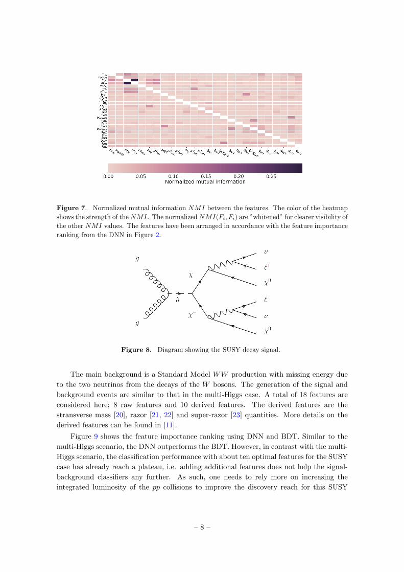
Figure 7. Normalized mutual information NMI between the features. The color of the heatmap

shows the strength of theNMI. The normalizedNMI(Fi, Fi) are ”whitened” for clearer visibility of

the other NMI values. The features have been arranged in accordance with the feature importance

ranking from the DNN in Figure 2.

Figure 8. Diagram showing the SUSY decay signal.

The main background is a Standard Model WW production with missing energy due

to the two neutrinos from the decays of the W bosons. The generation of the signal and

background events are similar to that in the multi-Higgs case. A total of 18 features are

considered here; 8 raw features and 10 derived features. The derived features are the

stransverse mass [20], razor [21, 22] and super-razor [23] quantities. More details on the

derived features can be found in [11].

Figure 9 shows the feature importance ranking using DNN and BDT. Similar to the

multi-Higgs scenario, the DNN outperforms the BDT. However, in contrast with the multi-

Higgs scenario, the classification performance with about ten optimal features for the SUSY

case has already reach a plateau, i.e. adding additional features does not help the signal-

background classifiers any further. As such, one needs to rely more on increasing the

integrated luminosity of the pp collisions to improve the discovery reach for this SUSY

– 8 –

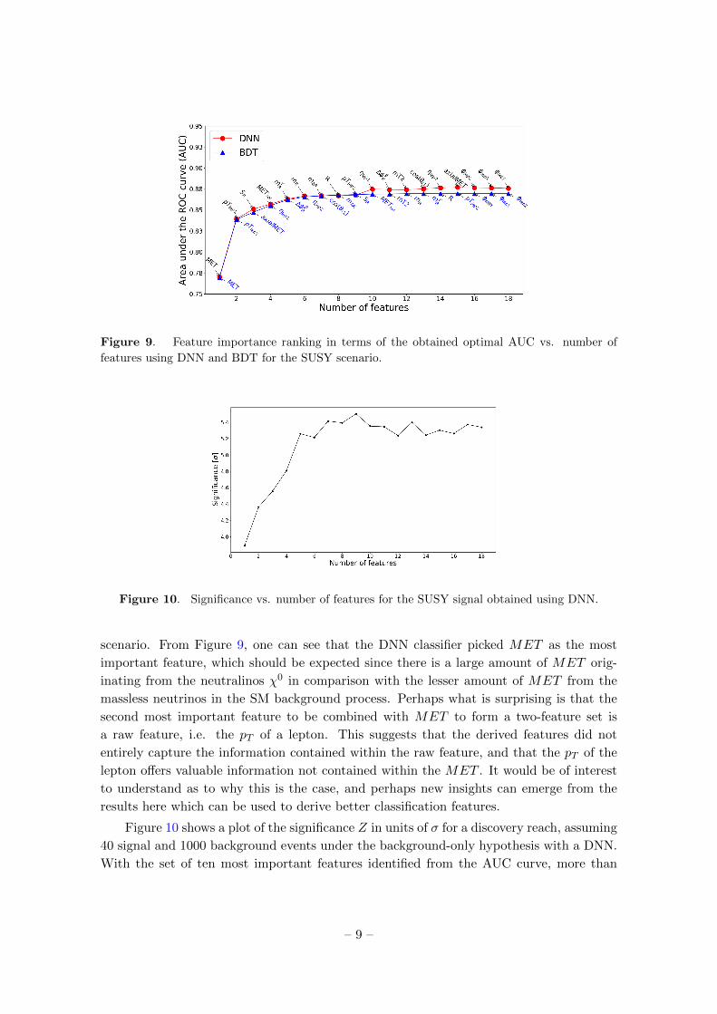
Figure 9. Feature importance ranking in terms of the obtained optimal AUC vs. number of

features using DNN and BDT for the SUSY scenario.

Figure 10. Significance vs. number of features for the SUSY signal obtained using DNN.

scenario. From Figure 9, one can see that the DNN classifier picked MET as the most

important feature, which should be expected since there is a large amount of MET orig-

inating from the neutralinos χ0 in comparison with the lesser amount of MET from the

massless neutrinos in the SM background process. Perhaps what is surprising is that the

second most important feature to be combined with MET to form a two-feature set is

a raw feature, i.e. the pT of a lepton. This suggests that the derived features did not

entirely capture the information contained within the raw feature, and that the pT of the

lepton offers valuable information not contained within the MET . It would be of interest

to understand as to why this is the case, and perhaps new insights can emerge from the

results here which can be used to derive better classification features.

Figure 10 shows a plot of the significance Z in units of σ for a discovery reach, assuming

40 signal and 1000 background events under the background-only hypothesis with a DNN.

With the set of ten most important features identified from the AUC curve, more than

– 9 –

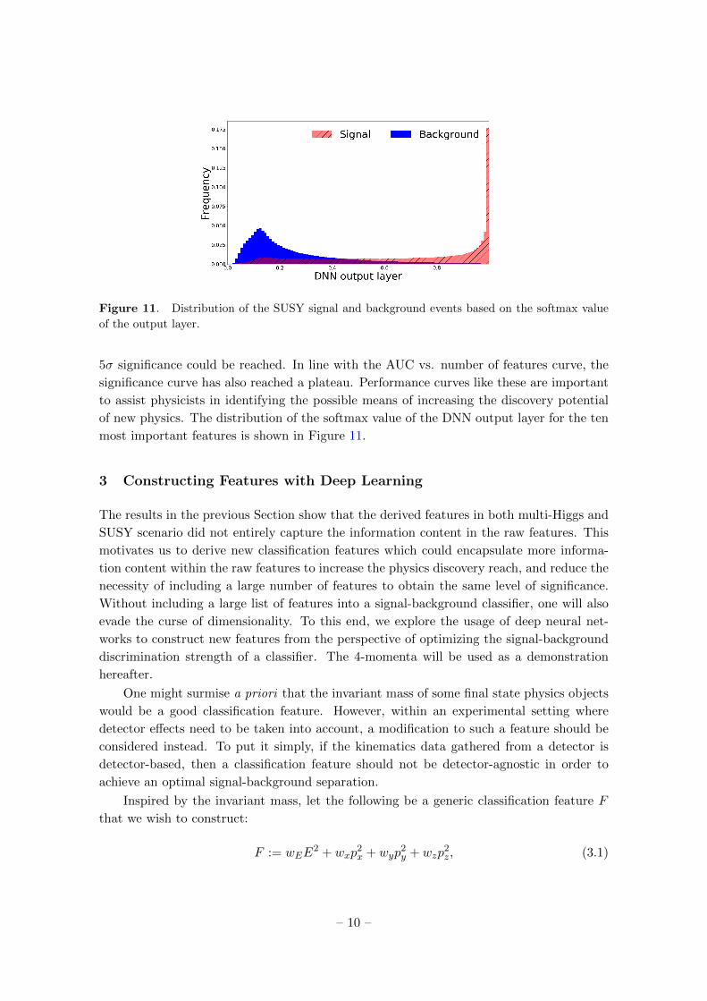
Figure 11. Distribution of the SUSY signal and background events based on the softmax value

of the output layer.

5σ significance could be reached. In line with the AUC vs. number of features curve, the

significance curve has also reached a plateau. Performance curves like these are important

to assist physicists in identifying the possible means of increasing the discovery potential

of new physics. The distribution of the softmax value of the DNN output layer for the ten

most important features is shown in Figure 11.

3 Constructing Features with Deep Learning

The results in the previous Section show that the derived features in both multi-Higgs and

SUSY scenario did not entirely capture the information content in the raw features. This

motivates us to derive new classification features which could encapsulate more informa-

tion content within the raw features to increase the physics discovery reach, and reduce the

necessity of including a large number of features to obtain the same level of significance.

Without including a large list of features into a signal-background classifier, one will also

evade the curse of dimensionality. To this end, we explore the usage of deep neural net-

works to construct new features from the perspective of optimizing the signal-background

discrimination strength of a classifier. The 4-momenta will be used as a demonstration

hereafter.

One might surmise a priori that the invariant mass of some final state physics objects

would be a good classification feature. However, within an experimental setting where

detector effects need to be taken into account, a modification to such a feature should be

considered instead. To put it simply, if the kinematics data gathered from a detector is

detector-based, then a classification feature should not be detector-agnostic in order to

achieve an optimal signal-background separation.

Inspired by the invariant mass, let the following be a generic classification feature F

that we wish to construct:

F := wEE2 + wxp

2x + wyp

2y + wzp

2z, (3.1)

– 10 –

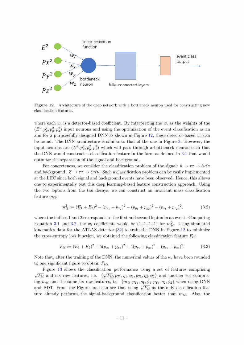
Figure 12. Architecture of the deep network with a bottleneck neuron used for constructing new

classification features.

where each wi is a detector-based coefficient. By interpreting the wi as the weights of the

(E2, p2x, p2y, p

2z) input neurons and using the optimization of the event classification as an

aim for a purposefully designed DNN as shown in Figure 12, these detector-based wi can

be found. The DNN architecture is similar to that of the one in Figure 3. However, the

input neurons are (E2, p2x, p2y, p

2z) which will pass through a bottleneck neuron such that

the DNN would construct a classification feature in the form as defined in 3.1 that would

optimize the separation of the signal and background.

For concreteness, we consider the classification problem of the signal: h→ ττ → `ν`ν

and background: Z → ττ → `ν`ν. Such a classification problem can be easily implemented

at the LHC since both signal and background events have been observed. Hence, this allows

one to experimentally test this deep learning-based feature construction approach. Using

the two leptons from the tau decays, we can construct an invariant mass classification

feature m``:

m2`` := (E1 + E2)

2 − (px1 + px2)2 − (py1 + py2)2 − (pz1 + pz2)2, (3.2)

where the indices 1 and 2 corresponds to the first and second lepton in an event. Comparing

Equation 3.1 and 3.2, the wi coefficients would be (1,-1,-1,-1) for m2``. Using simulated

kinematics data for the ATLAS detector [32] to train the DNN in Figure 12 to minimize

the cross-entropy loss function, we obtained the following classification feature F``:

F`` := (E1 + E2)2 + 5(px1 + px2)2 + 5(py1 + py2)2 − (pz1 + pz2)2. (3.3)

Note that, after the training of the DNN, the numerical values of the wi have been rounded

to one significant figure to obtain F``.

Figure 13 shows the classification performance using a set of features comprising√F`` and six raw features, i.e. {

√F``, pT1 , η1, φ1, pT2 , η2, φ2} and another set compris-

ing m`` and the same six raw features, i.e. {m``, pT1 , η1, φ1, pT2 , η2, φ2} when using DNN

and BDT. From the Figure, one can see that using√F`` as the only classification fea-

ture already performs the signal-background classification better than m``. Also, the

– 11 –

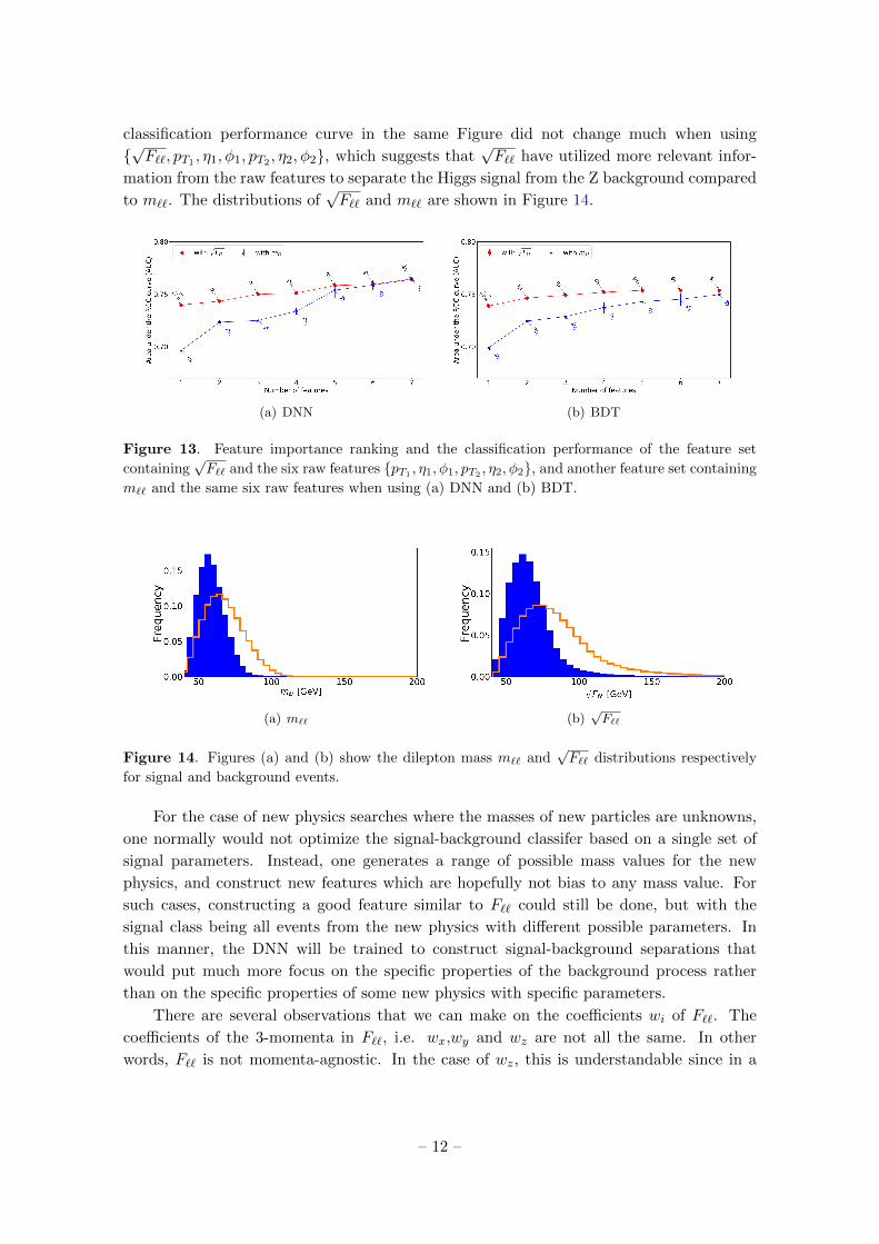
classification performance curve in the same Figure did not change much when using

{√F``, pT1 , η1, φ1, pT2 , η2, φ2}, which suggests that

√F`` have utilized more relevant infor-

mation from the raw features to separate the Higgs signal from the Z background compared

to m``. The distributions of√F`` and m`` are shown in Figure 14.

(a) DNN (b) BDT

Figure 13. Feature importance ranking and the classification performance of the feature set

containing√F`` and the six raw features {pT1

, η1, φ1, pT2, η2, φ2}, and another feature set containing

m`` and the same six raw features when using (a) DNN and (b) BDT.

(a) m`` (b)√F``

Figure 14. Figures (a) and (b) show the dilepton mass m`` and√F`` distributions respectively

for signal and background events.

For the case of new physics searches where the masses of new particles are unknowns,

one normally would not optimize the signal-background classifer based on a single set of

signal parameters. Instead, one generates a range of possible mass values for the new

physics, and construct new features which are hopefully not bias to any mass value. For

such cases, constructing a good feature similar to F`` could still be done, but with the

signal class being all events from the new physics with different possible parameters. In

this manner, the DNN will be trained to construct signal-background separations that

would put much more focus on the specific properties of the background process rather

than on the specific properties of some new physics with specific parameters.

There are several observations that we can make on the coefficients wi of F``. The

coefficients of the 3-momenta in F``, i.e. wx,wy and wz are not all the same. In other

words, F`` is not momenta-agnostic. In the case of wz, this is understandable since in a

– 12 –

detector environment, one already anticipates that the longitudinal momentum would not

be similar to the transverse momenta. As for the wx and wy coefficients, they are the same

to one significant figure. This suggests that there is no bias in the transverse momenta.

We did a check on this with a convolutional neural network to find out if the transverse

momenta px and py are indeed indistinguishable from one another. In this manner, the

convolutional neural network (CNN) acts as a momentum bias checking tool.

We first define our signal and background classes. Assuming the data points of (px1 +

px2) vs. (py1 + py2) came from an unknown distribution, we define our signal to be scatter

plots of (px1 + px2) vs. (py1 + py2), and a swap of the axes as the background, i.e. the

scatter plots of (py1 + py2) vs. (px1 + px2). A representative example of a signal and a

background scatter plot is shown in Figure 16(a). Each scatter plot contains the momenta

(a) (b)

Figure 15. Figure (a) shows a scatter plot of the signal (px1+px2

) vs. (py1+py2

) and background

(py1+ py2

) vs. (px1+ px2

). Figure (b) shows an image of (px1+ px2

) vs. (py1+ py2

) converted from

the scatter plot signal used in Figure (a).

from N events randomly selected from the existing Monte Carlo dataset. In our work, we

chose N as 10 thousand. Since the inputs to the CNN have to be images, we converted

each scatter plot to an image with 20 x 20 pixels (see Figure 16(b)). Using a simple

CNN with one convolution layer with 2x2 filters and two fully-connected layers, we find

a classification accuracy of 0.5 ± 0.006 indicating that the CNN basically made random

classifications, i.e. the CNN could find any bias in the transverse plane when comparing pxvs. py. Had if there was any bias, the CNN would be able to distinguish the signals from

backgrounds. Rpeating this procedure with the signal being (px1 + px2) vs. (pz1 + pz2) and

the background being (pz1 + pz2) vs. (px1 + px2) (see Figure 16), we find a classification

accuracy of 1, indicating that the CNN regards the transverse momentum and longitudinal

momentum as being entirely different from one another.

– 13 –

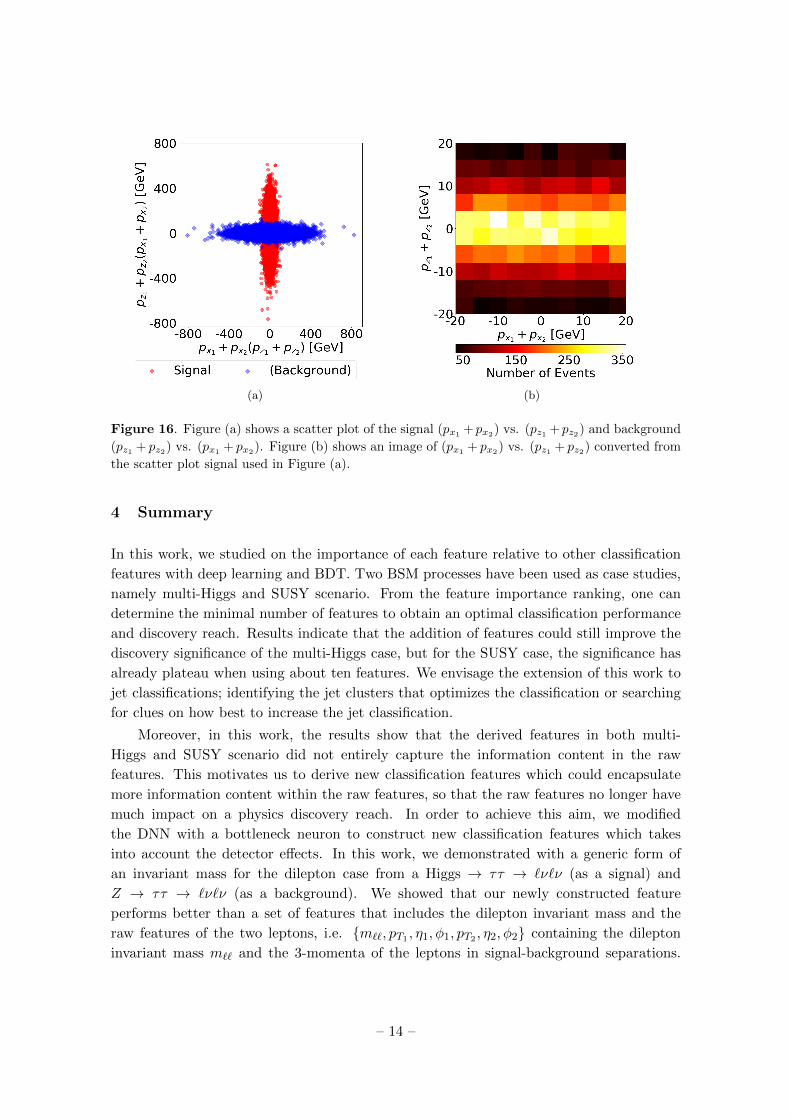
(a) (b)

Figure 16. Figure (a) shows a scatter plot of the signal (px1 + px2) vs. (pz1 + pz2) and background

(pz1 + pz2) vs. (px1+ px2

). Figure (b) shows an image of (px1+ px2

) vs. (pz1 + pz2) converted from

the scatter plot signal used in Figure (a).

4 Summary

In this work, we studied on the importance of each feature relative to other classification

features with deep learning and BDT. Two BSM processes have been used as case studies,

namely multi-Higgs and SUSY scenario. From the feature importance ranking, one can

determine the minimal number of features to obtain an optimal classification performance

and discovery reach. Results indicate that the addition of features could still improve the

discovery significance of the multi-Higgs case, but for the SUSY case, the significance has

already plateau when using about ten features. We envisage the extension of this work to

jet classifications; identifying the jet clusters that optimizes the classification or searching

for clues on how best to increase the jet classification.

Moreover, in this work, the results show that the derived features in both multi-

Higgs and SUSY scenario did not entirely capture the information content in the raw

features. This motivates us to derive new classification features which could encapsulate

more information content within the raw features, so that the raw features no longer have

much impact on a physics discovery reach. In order to achieve this aim, we modified

the DNN with a bottleneck neuron to construct new classification features which takes

into account the detector effects. In this work, we demonstrated with a generic form of

an invariant mass for the dilepton case from a Higgs → ττ → `ν`ν (as a signal) and

Z → ττ → `ν`ν (as a background). We showed that our newly constructed feature

performs better than a set of features that includes the dilepton invariant mass and the

raw features of the two leptons, i.e. {m``, pT1 , η1, φ1, pT2 , η2, φ2} containing the dilepton

invariant mass m`` and the 3-momenta of the leptons in signal-background separations.

– 14 –

Since the Higgs and Z decay to ττ have already been observed at the LHC, our feature

construction approach can be readily tested in the experiments. It is straightforward to

extend the feature construction approach to new physics searches.

As a side application of the feature construction approach, we could use the resulting

constructed feature to identify any momentum biases. In this work, we have also used

a convolutional neural network as part of the momentum bias checking approach. We

performed a demonstration using the sum of the px and py momenta of the two leptons, and

the sum of the px and pz momenta of the same two leptons. In particular, the convolutional

neural network gives an accuracy of 0.5 if two variables are statistically indistinguishable,

and an accuracy of 1 if two variables are statistically distinguishable.

Acknowledgments

We wish to express our gratitude to Shen-Jian Chen and Zuo-Wei Liu for providing the com-

puting facilities, including an Nvidia Tesla P40 GPU to complete this work. The authors

gratefully acknowledge the support of the International Science and Technology Coopera-

tion Program of China (Grant No. 2015DFG02100) and the National 973 Project Founda-

tion of the Ministry of Science and Technology of China (Contract No. 2013CB834300).

References

[1] ATLAS collaboration, G. Aad et al., Observation of a new particle in the search for the

Standard Model Higgs boson with the ATLAS detector at the LHC, Phys. Lett. B 716 (2012)

1 – 29.

[2] CMS collaboration, S. Chatrchyan et al., Observation of a new boson at a mass of 125 GeV

with the CMS experiment at the LHC, Phys. Lett. B 716 (2012) 30 – 61.

[3] AtlAS collaboration, G. Aad et al., Search for a multi-Higgs-boson cascade in WWbb events

with the ATLAS detector in pp collisions at√s = 8 TeV, Phys. Rev. D 89 (2014) .

[4] B. P. Roe et al., Boosted decision trees as an alternative to artificial neural networks for

particle identification, NIM A 543 (2005) 577 – 584.

[5] Y. Lecun, Y. Bengio and G. Hinton, Deep learning, Nature 521 (2015) 436 – 444.

[6] L. A. .Gatys, A. S. Ecker and M. Bethge, Texture and art with deep neural networks, Current

Opinion in Neurobiology 46 (2017) 178 – 186.

[7] A. Karpathy and L. Fei-Fei, Deep Visual-Semantic Alignments for Generating Image

Descriptions, IEEE Trans. Pattern Anal. Mach. Intell. 39 (Apr., 2017) 664–676.

[8] M. K. K. Leung, H. Y. Xiong, L. J. Lee and B. J. Frey, Deep learning of the tissue-regulated

splicing code, Bioinformatics 30 (2014) i121–i129.

[9] P. Mamoshina, A. Vieira, E. Putin and A. Zhavoronkov, Applications of Deep Learning in

Biomedicine, Molecular Pharmaceutics 13 (2016) 1445–1454.

[10] C. Madrazo, I. Cacha, L. Iglesias and J. de Lucas, Application of a Convolutional Neural

Network for image classification to the analysis of collisions in High Energy Physics, 2017,

1708.07034.

– 15 –

[11] P. Baldi, P. Sadowski and D. Whiteson, Searching for Exotic Particles in High-Energy

Physics with Deep Learning, Nature Commun. 5 (2014) 4308.

[12] P. Baldi, K. Bauer, C. Eng, P. Sadowski and D. Whiteson, Jet Substructure Classification in

High-Energy Physics with Deep Neural Networks, Phys. Rev. D93 (2016) 094034.

[13] P. T. Komiske, E. M. Metodiev and M. D. Schwartz, Deep learning in color: towards

automated quark/gluon jet discrimination, JHEP 01 (2017) 110.

[14] L. de Oliveira, M. Kagan, L. Mackey, B. Nachman and A. Schwartzman, Jet-images — deep

learning edition, JHEP 2016 (2016) 69.

[15] M. Wielgosz, A. Skocze and M. Mertik, Using LSTM recurrent neural networks for

monitoring the LHC superconducting magnets, Nucl. Instrum. Meth. A867 (2017) 40–50.

[16] G. E. Hinton and R. S. Zemel, Autoencoders, Minimum Description Length and Helmholtz

Free Energy, in Advances in Neural Information Processing Systems 6 (J. D. Cowan,

G. Tesauro and J. Alspector, eds.), pp. 3–10. Morgan-Kaufmann, 1994.

[17] A. Krizhevsky, I. Sutskever and G. E. Hinton, ImageNet Classification with Deep

Convolutional Neural Networks, Commun. ACM 60 (May, 2017) 84–90.

[18] S. Hochreiter and J. Schmidhuber, Long Short-Term Memory, Neural Comput. 9 (1997)

1735–1780.

[19] P. Frasconi, M. Gori and A. Sperduti, A General Framework for Adaptive Processing of Data

Structures, Trans. Neur. Netw. 9 (Sept., 1998) 768–786.

[20] A. Barr, C. Lester and P. Stephens, m(T2): The Truth behind the glamour, J. Phys. G29

(2003) 2343–2363.

[21] C. Rogan, Kinematical variables towards new dynamics at the LHC, 2017, 1006.2727.

[22] CMS collaboration, S. Chatrchyan et al., Inclusive search for squarks and gluinos in pp

collisions at√s = 7 TeV, Phys. Rev. D85 (2012) 012004.

[23] M. R. Buckley, J. D. Lykken, C. Rogan and M. Spiropulu, Super-Razor and Searches for

Sleptons and Charginos at the LHC, Phys. Rev. D89 (2014) 055020.

[24] A. Djouadi, The Anatomy of electro-weak symmetry breaking. II. The Higgs bosons in the

minimal supersymmetric model, Phys. Rept. 459 (2008) 1–241.

[25] ATLAS collaboration, G. Aad et al., Evidence for the Higgs-boson Yukawa coupling to tau

leptons with the ATLAS detector, JHEP 04 (2015) 117.

[26] CMS collaboration, S. Chatrchyan et al., Evidence for the 125 GeV Higgs boson decaying to

a pair of τ leptons, JHEP 05 (2014) 104.

[27] J. Alwall, R. Frederix, S. Frixione, V. Hirschi, F. Maltoni, O. Mattelaer et al., The

automated computation of tree-level and next-to-leading order differential cross sections, and

their matching to parton shower simulations, JHEP 2014 (2014) 79.

[28] T. Sjostrand, S. Mrenna and P. Z. Skands, PYTHIA 6.4 Physics and Manual, JHEP 05

(2006) 026.

[29] DELPHES 3 collaboration, J. de Favereau, C. Delaere, P. Demin, A. Giammanco,

V. Lematre, A. Mertens et al., DELPHES 3, A modular framework for fast simulation of a

generic collider experiment, JHEP 02 (2014) 057.

[30] L. Breiman, Random forests, Machine Learning 45 (2001) 5–32.

– 16 –

[31] G. Cowan, K. Cranmer, E. Gross and O. Vitells, Asymptotic formulae for likelihood-based

tests of new physics, Eur. Phys. J. C 71 (2011) 1554.

[32] P. Baldi, P. Sadowski and D. Whiteson, Enhanced Higgs Boson to τ+τ− Search with Deep

Learning, Phys. Rev. Lett. 114 (2015) 111801.

– 17 –