Embed Size (px)
Citation preview
Improved sampling in Monte Carlo simulations of small
clusters
by
Hanbin Liu
BS, Tianjin University, 1996
MS, Tsinghua University, 1999
Submitted to the Graduate Faculty of
Arts and Science in partial fulfillment
of the requirements for the degree of
Doctor of Philosophy
University of Pittsburgh
[2005]
UNIVERSITY OF PITTSBURGH
FACULTY OF ARTS AND SCIENCES
This dissertation was presented
by
Hanbin Liu
It was defended on
July 5th, 2005
and approved by
Rob D. Coalson
David W. Pratt
Jeffery D. Madura
Kenneth D. Jordan
Dissertation Director
ii
Advisor: Professor Kenneth D. Jordan
Improved sampling in Monte Carlo simulations of small clusters
Hanbin Liu, PhD
University of Pittsburgh, 2005
In this thesis, improved sampling algorithms are applied to atomic and molecular
clusters. The parallel-tempering Monte Carlo procedure is used to characterize the
(CO2)n, n = 6, 8, 13, 19, and 38, clusters. The heat capacity curves of the n = 13 and 19
clusters are found to have pronounced peaks that can be associated with cluster melting.
In addition, there is evidence of a low temperature “solid ↔ solid” transition in the case
of (CO2)19. The low-energy minima and rearrangement pathways are determined and
used to examine the complexity of the potential energy surfaces of the clusters.
An algorithm combining the Tsallis generalized ensemble and the parallel
tempering algorithm is introduced and applied to a 1D model potential and to Ar38. The
convergence of parallel tempering Monte Carlo simulations of the 38-atom Lennard-
Jones cluster starting from the Oh global minimum and from the C5v second lowest-
energy minimum is also investigated. It is found that achieving convergence is
appreciably more difficult, particularly at temperatures in the vicinity of the Oh C5v
transformation, when starting from the C5v structure. Compared to PTMC, the hybrid
algorithm is about 10 times faster for reaching equilibrium in the 1D model potential and
is about 3 times faster for reaching equilibrium in the LJ38 system when starting from the
iii

second lowest energy minimum. The Wang-Landau free random walk algorithm is also
applied to Ar13 and Ar38.
iv

TABLE OF CONTENTS 1. Chapter 1 Introduction ................................................................................................ 1
1.1. The Monte Carlo method .................................................................................... 1 1.2. Statistical Mechanics of equilibrium systems5 ................................................... 1
1.2.1. Master equation and equilibrium state........................................................ 1 1.2.2. Fluctuations of energy in Monte Carlo simulations.................................... 3
1.3. Principles of Monte Carlo simulations and the Metropolis algorithm................ 3 1.4. Problem of quasi-ergodicity and advanced Monte Carlo algorithms ................. 6
1.4.1. Jump walking and parallel tempering Monte Carlo algorithm ................... 6 1.4.2. Multicanonical Monte Carlo algorithm ...................................................... 7 1.4.3. Tsallis statistics ........................................................................................... 9 1.4.4. Wang-Landau free random walk in energy space..................................... 11 1.4.5. Other methods........................................................................................... 11
1.5. The overview of the thesis and application of advanced sampling algorithms 12 2. Chapter 2 Finite temperature properties of (CO2)n clusters ...................................... 15
2.1. Introduction....................................................................................................... 15 2.2. Methodology..................................................................................................... 16
2.2.1. Model potential ......................................................................................... 16 2.2.2. Parallel tempering Monte Carlo procedure............................................... 18 2.2.3. Disconnectivity graphs.............................................................................. 21
2.3. Results............................................................................................................... 21 i) (CO2)6 .................................................................................................................... 22 ii) (CO2)8 ................................................................................................................... 23 iii) (CO2)13................................................................................................................. 24 iv) (CO2)19................................................................................................................. 25 v) (CO2)38 .................................................................................................................. 27
2.4. Conclusions....................................................................................................... 27 3. Chapter 3 On the Convergence of Parallel Tempering Monte Carlo Simulations of LJ38................................................................................................................................................................................................... 45
3.1. Introduction....................................................................................................... 45 3.2. Methodology..................................................................................................... 47
3.2.1. PTTS algorithm......................................................................................... 47 3.2.2. Reweight technology ................................................................................ 48
3.3. Computational details ....................................................................................... 50 3.3.1. 1D model potential.................................................................................... 50 3.3.2. PTMC simulations of Ar38 ........................................................................ 51 3.3.3. PTTS simulations of Ar38.......................................................................... 52
3.4. Results............................................................................................................... 52 3.4.1. 1D model potential.................................................................................... 52 3.4.2. PTMC simulations of Ar38 ........................................................................ 53 3.4.3. PTTS simulations of Ar38.......................................................................... 57
3.5. Conclusions....................................................................................................... 58
v
4. Chapter 4 The application of Wang-Laudau free random walk algorithm on Ar cluster................................................................................................................................ 72
4.1. Introduction....................................................................................................... 72 4.2. Method .............................................................................................................. 73 4.3. Simulation details.............................................................................................. 74 4.4. Results and discussion ...................................................................................... 75
BIBLIOGRAPHY............................................................................................................. 78 Appendix A................................................................................................................... 84 Computational study about the stereochemistry of the cyclization of a secondary alkyllithium................................................................................................................... 84 I. Introduction ............................................................................................................... 84 II. Computational details............................................................................................... 85 III. Result and Discussion ............................................................................................. 86 IV. Conclusions............................................................................................................. 88 References..................................................................................................................... 90 Appendix B ................................................................................................................... 98 Theoretical characterization of the (H2O)21 cluster....................................................... 98 I. Introduction ............................................................................................................... 99 II. Computational details............................................................................................. 100 III. Results and Discussion ......................................................................................... 101 IV. Conclusions........................................................................................................... 103 References................................................................................................................... 105
vi

LIST OF TABLES
Table 2.1 Location of the point charges in the Murthy CO2 potential.............................. 17
Table 2.2 Lennard-Jones parameters for the Murthy CO2 model potentiala..................... 17
vii
LIST OF FIGURES
Figure 1.1 Schematic of the parallel tempering algorithm. Simulations at the N temperatures of interest, T1,T2…TN are carried out in parallel, one temperature per processor. In each simulation, most moves are carried out with the Metropolis algorithm, represented by the filled circles, and the remaining moves involve exchanges, represented by the unfilled rectangles, between the configurations at adjacent temperatures. The figure was adapted from Arnold Tharrington’s thesis. . 14
Figure 2.1 Heat capacity curves of the (CO2)n clusters calculated by means of parallel tempering Monte Carlo simulations. For each cluster, run1 denotes the simulation starting from global minimum and run2 denotes the simulation starting from a random geometry. ..................................................................................................... 29
Figure 2.2 Energy level diagram for the (CO2)n clusters. Each horizontal line corresponds to the energy of a local minimum as determined from quenching calculations. ...... 30
Figure 2.3 Structures of the six lowest-energy minima of (CO2)6 from eigenmode-following optimizations. ........................................................................................... 31
Figure 2.4 Distributions of local minima generated by quenching configurations from parallel tempering Monte Carlo simulations on (CO2)6............................................ 32
Figure 2.5 Disconnectivity graph for the (CO2)6 cluster. The numbers designate the low-energy structures depicted in Figure 2.3. .................................................................. 33
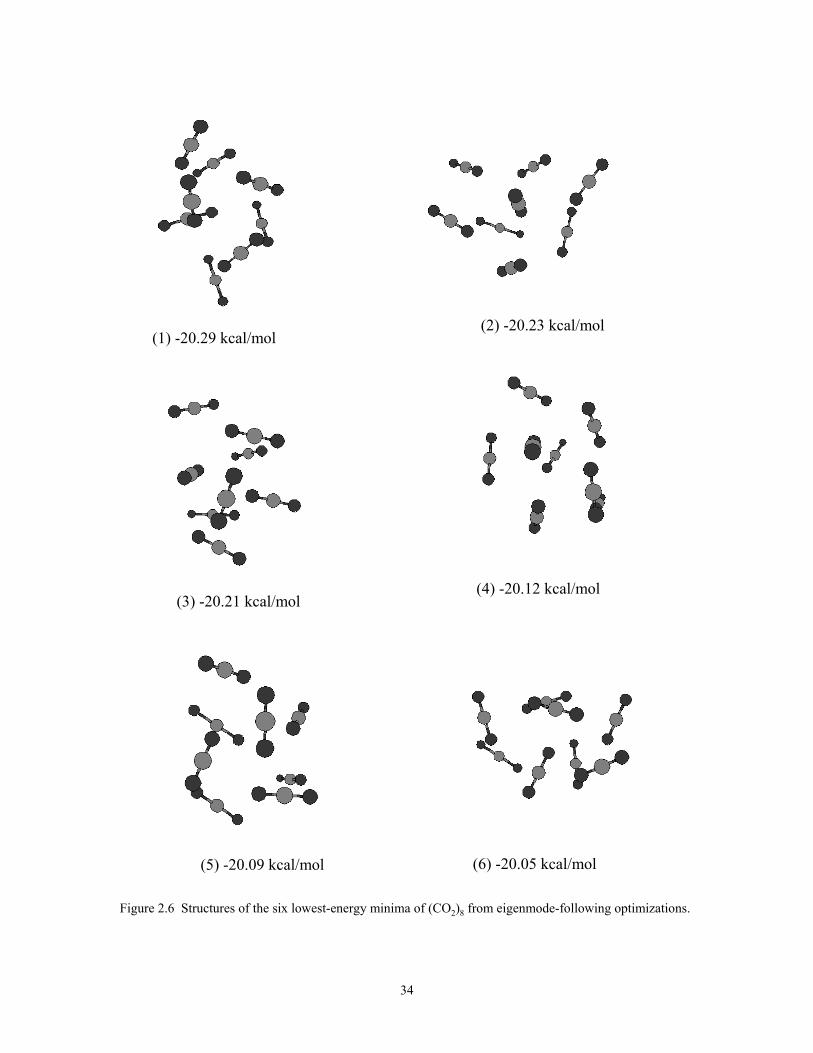
Figure 2.6 Structures of the six lowest-energy minima of (CO2)8 from eigenmode-following optimizations. ........................................................................................... 34
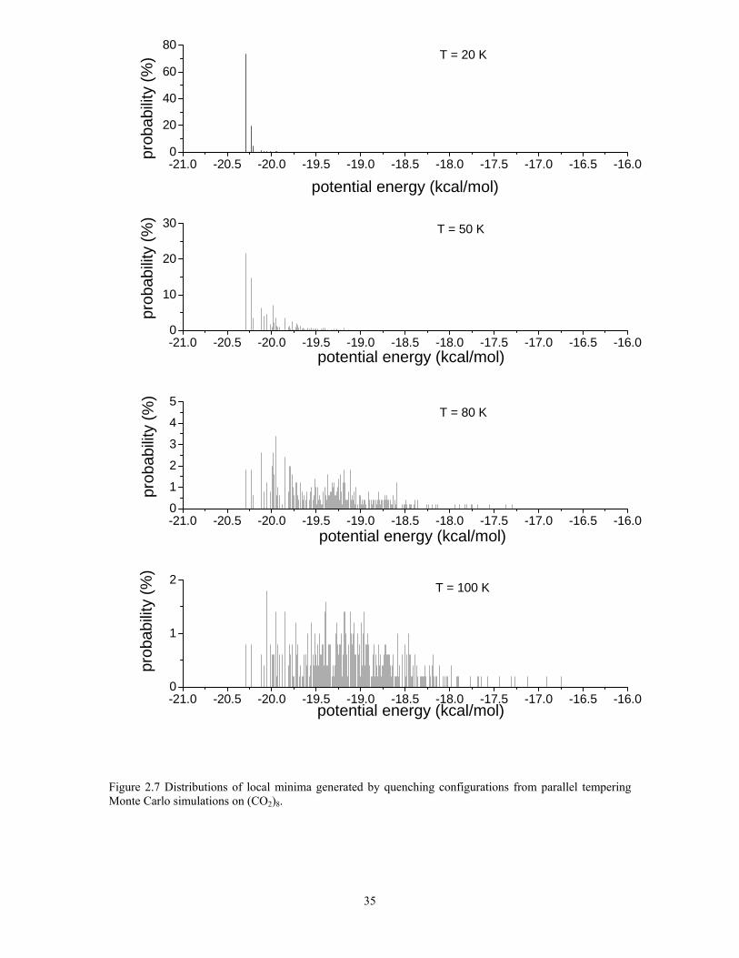
Figure 2.7 Distributions of local minima generated by quenching configurations from parallel tempering Monte Carlo simulations on (CO2)8............................................ 35
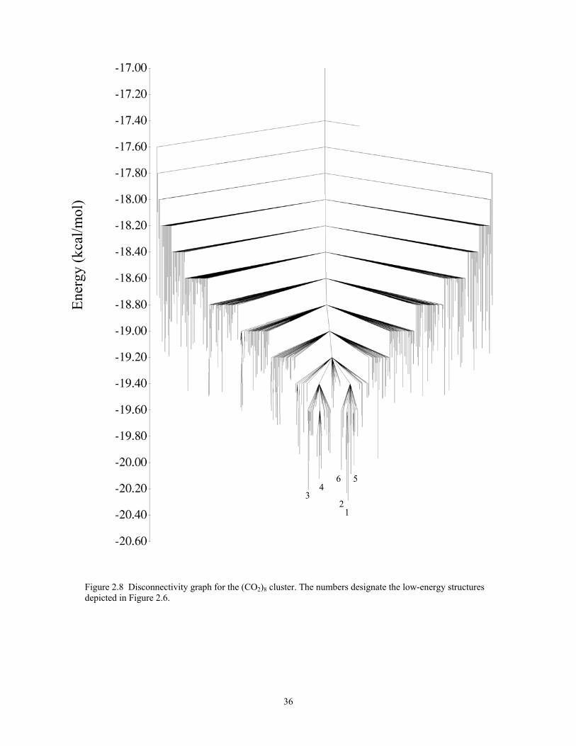
Figure 2.8 Disconnectivity graph for the (CO2)8 cluster. The numbers designate the low-energy structures depicted in Figure 2.6. .................................................................. 36
Figure 2.9 Structures of the six lowest-energy minima of (CO2)13 from eigenmode-following optimizations. ........................................................................................... 37
Figure 2.10 Distributions of local minima generated by quenching configurations from parallel tempering Monte Carlo simulations on (CO2)13. ......................................... 38
Figure 2.11 Disconnectivity graph for the (CO2)13 cluster. The numbers designate the low-energy structures depicted in Figure 2.9............................................................ 39
viii

Figure 2.12 Structures of the six lowest-energy minima of (CO2)19 from eigenmode-following optimizations. ........................................................................................... 40
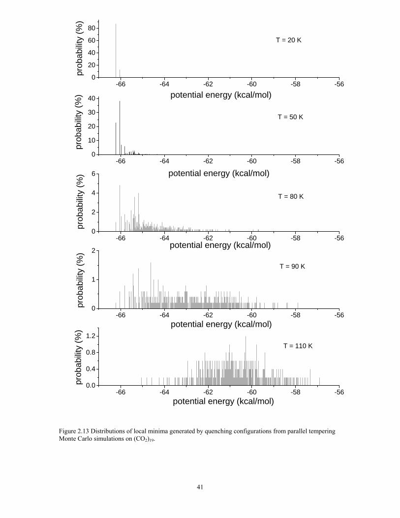
Figure 2.13 Distributions of local minima generated by quenching configurations from parallel tempering Monte Carlo simulations on (CO2)19. ......................................... 41
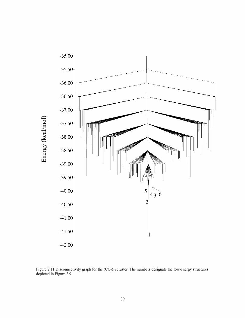
Figure 2.14 Disconnectivity graph for the (CO2)19 cluster. The numbers designate the low-energy structures depicted in Figure 2.12.......................................................... 42
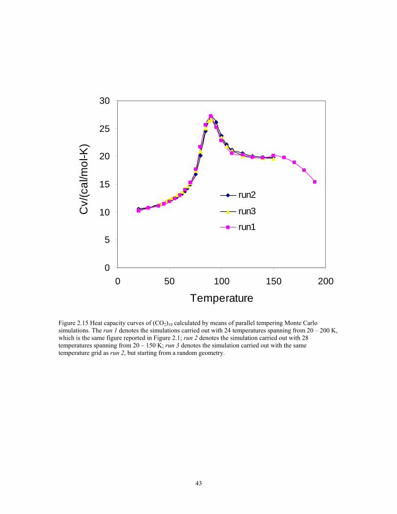
Figure 2.15 Heat capacity curves of (CO2)19 calculated by means of parallel tempering Monte Carlo simulations. The run 1 denotes the simulations carried out with 24 temperatures spanning from 20 – 200 K, which is the same figure reported in Figure 2.1; run 2 denotes the simulation carried out with 28 temperatures spanning from 20 – 150 K; run 3 denotes the simulation carried out with the same temperature grid as run 2, but starting from a random geometry. ............................................................ 43
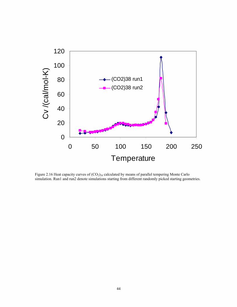
Figure 2.16 Heat capacity curves of (CO2)38 calculated by means of parallel tempering Monte Carlo simulation. Run1 and run2 denote simulations starting from different randomly picked starting geometries. ....................................................................... 44
Figure 3.1 Disconnectivity diagram of Ar38. .................................................................... 60
Figure 3.2 Two lowest energy isomers of Ar38................................................................. 61
Figure 3.3 One-dimensional potential energy V(x) vs. position x and the analytical distributions ρ1 and ρ2 at T = 24 and 0.094, respectively. ......................................... 62
Figure 3.4 Ergodicity of the various simulation methods for the one-dimensional model and T= 0.093. MMC denotes Metropolis Monte Carlo algorithm, TS denotes Tsallis statistics, PTMC denotes parallel tempering Monte Carlo, and PTTS denotes parallel tempering Tsallis statistics........................................................................................ 63
Figure 3.5 Ergodicity for the various simulation methods for the one-dimensional model at different temperatures. MMC denotes Metropolis Monte Carlo algorithm, TS denotes Tsallis statistics, PTMC denotes parallel tempering Monte Carlo, and PTTS denotes parallel tempering Tsallis statistics.............................................................. 64
Figure 3.6 Heat capacity vs. T of Ar38 from PTMC simulations starting from the global minimum isomer. All production runs were carried out for 1 billion moves. Equilibrium periods ranged from 0.4 to 6.4x10⁹. ..................................................... 65
Figure 3.7 Heat capacity vs. T of Ar38 from PTMC simulations starting from second lowest energy minimum isomer. All production runs were carried out for 1 billion moves. Equilibrium periods ranged from 0.4 to 6.4x10⁹.......................................... 66
Figure 3.8 Heat capacity vs. T of Ar38 from PTMC simulations starting from the global minimum and from the second lowest energy isomer. The equilibrium periods were 3.4x10⁹ moves, and the production runs were carried out for 4x10⁹ moves. ........... 67
ix

Figure 3.9 Inherent structures at the end of various length equilibration periods for PTMC simulations of Ar38: (a) starting from the global minimum, (b) starting from the second lowest energy minimum. The number of moves in each equilibration period is specified in the figure............................................................................................ 68
Figure 3.10 Inherent structure distributions from PTMC simulations of Ar38 starting from the second lowest energy minimum. Simulations were carried out with a production period of 1×10⁹ moves and differ in the length of the equilibrium period. The inherent structures are labeled as follows: E = -41.821 (■), -41.659 (●), -41.630 (▲), -41.588 (▼), -41.569 (♦) and > -41.569 kcal/mol (+). The inherent structures with energies of -41.821 and -41.659 kcal/mol are the global minimum and the second lowest energy minimum, respectively. ......................................................... 69
Figure 3.11 Inherent structure distributions from PTMC simulations of Ar38 starting from: (a) the global minimum and (b) the second lowest energy minimum. The simulations were carried out with an equilibration period of 3.4x10⁹ moves and production runs of 4x10⁹ moves. The inherent structures are labeled as follows: E = -41.821 (■), -41.659 (●), -41.630 (▲), -41.588 (▼), -41.569 (♦) and > -41.569 kcal/mol (+).... 70
Figure 3.12 Heat capacity vs. T of Ar38 from PTTS simulations starting from the second lowest energy minimum. Equilibration periods ranged from 0.4x10⁸ to 2.6x10⁹ moves, and production periods were 1x10⁹ moves for the case of an equilibration period of 0.4x10⁸ moves and 0.6x10⁹ moves in the other four cases. ...................... 71
Figure 4.1 Heat capacity vs. temperature curves of the Ar13 cluster. The blue line denotes the result obtained using the WL algorithm, the purple line denotes results obtained using the jump walk algorithm. ................................................................................ 76
Figure 4.2 Heat capacity vs. temperature curve of Ar38 obtained using the WL algorithm and PTTS algorithm.................................................................................................. 77
x

PREFACE
First and foremost, I would like to thank my advisor Ken Jordan with my deepest
gratitude. He guided me into the wonderful area of computational chemistry. He is
always there to help when I have difficulties in my research. Besides his comprehensive
knowledge in chemistry, his zeal for science, work ethic, patience and life attitude
impressed me a lot. He serves as my role model of a scientist and an educator.
I would also like to thank Professors Rob Coalson, David Pratt and Jeffery
Madura for serving on my thesis committee and Professor Maria Kurnikova at Carnegie
Mellon University for stimulating discussions on my proposal project. Their willingness
to share their expertise and provide valuable advice is greatly appreciated.
I want to thank all the members in Jordan group, past or present, for their help and
friendship. Especially, I want to thank Drs. Arnold Tharrington and Dominic Alfonso for
there valuable help when I just started my research here; Dr. Feng Wang and Dr. Richard
Christie, Brad M-K Tsai, Jun Cui, Kadir Diri, and Alex Bayden helped me a lot in many
valuable discussions. I enjoyed working with all the members of Jordan group and expect
to be a life long friend with them.
I want to thank my family, whose constant love and understanding supports me
during the past five years. I thank my husband Kai Deng for his encouraging and love. I
thank my parents, my sister Hantao and her family for their unconditional love and help. I
would not be able to obtain this degree without my family’s support. I am proud to be
the Mom of my son David Deng. He was born and grew up with me during my PhD
study at Pittsburgh. He is a great gift from God. I would like to thank God for everything.
xi

1. Chapter 1 Introduction
1.1. The Monte Carlo method
Monte Carlo simulation methods are used routinely in many fields, including
chemistry, biology, physics, engineering, and economics. The name “Monte Carlo” was
coined by Metropolis (inspired by Ulam's interest in poker) during the Manhattan Project
of World War II at Los Alamos1,2.
The basic idea in Monte Carlo simulations is to simulate the random fluctuation
of a system from state to state. In a Monte Carlo simulation, we directly simulate this
process, creating a model on our computer and making it pass through a sequence of
states in such a way that the probability of being in any particular state u at a given time t
is equal to the weight Wu(t) which that state would have in a real system. The advantage
of the Monte Carlo approach in statistical mechanics is that we only need to sample a
small fraction of the states of the system in order to obtain accurate estimates of the
partition function. 3-5
1.2. Statistical Mechanics of equilibrium systems5
1.2.1. Master equation and equilibrium state
Suppose that )( νµ →P is the rate of the transition from state µ to state ν, and
)(tµω represents the probability that the system will be in state µ at time t. Then the
master equation for the evolution of )(tµω in terms of the rates )( νµ →P can be written
as:
)].()()()([ νµωµνωω
νµν
µ →−→=∑ PtPtdt
d (1.1)
1
The first term on the right-hand side of this equation represents the rate of transitions into
state µ, and the second term represents the rate of transitions out of state µ. The
probabilities )(tµω obey the sum rule
1)( =∑ tµ
µω . (1.2)
If the system reaches equilibrium, then 0=dt
d µω , and the weights of all states become
constant.
Gibbs showed that for a system in thermal equilibrium with a reservoir at
temperature T, the equilibrium occupation probabilities are
µβµ
EeZ
p −=1 , (1.3)
where β denotes 1/kT, k is the Boltzmann constant and Z is the partition function. For an
equilibrium state, the probability distribution is known as the Boltzmann distribution.
From Equation 1.3, the expectation of an observable Q for a system in
equilibrium is
∑ −=µ
βµ
µEeQQΖ
1 . (1.4)
Based on Equation 1.4, the internal energy, heat capacity, entropy, and Helmholtz free
energy, F, of the system can be expressed
,11β
µβ
µµ ∂
∂−== −∑ Z
Z ZeEU E (1.5)
,log2
222
ββ
ββ
∂∂
=∂∂
−=∂∂
=ZkUk
TUC (1.6)
,loglogZ
Z kkS +∂
∂−=
ββ (1.7)
2
and
ZkTTSUF log−=−= . (1.8)
In performing Monte Carlo simulations, one often calculates the quantities of interest
directly without first evaluating the partition function.
1.2.2. Fluctuations of energy in Monte Carlo simulations
For studies of phase changes, it is useful to calculate the energy fluctuations,
which are given by
222)( EEEE −=− , (1.9)
since
2
222 11
βµ
βµ
µ
∂∂
== ∑ − ZZ
eEZ
E E . (1.10)
Combining Equations 1.6 and 1.9, we get
222
βkCEE =− . (1.11)
This shows that the heat capacity is proportional to the energy fluctuations of the
equilibrium system.
1.3. Principles of Monte Carlo simulations and the Metropolis algorithm
The Monte Carlo method in statistical mechanics generally uses Markov chains to
sample a state (or configuration) C with a probability P(C) to replace multivariate
integrations
∑=C
CPCff )()( (1.12)
by simple averages
3
)(11∑=
≅M
iiCf
Mf . (1.13)
It is very important to generate an appropriate random set of states according to the
Boltzmann probability. In a Markov process, given a system in one state µ, the
probability of accept moves from state µ to ν is only based on the state µ. Almost all
Monte Carlo schemes rely on Markov processes for generating the set of states used,
since it is impossible to choose states at random and accept or reject them with a
probability proportional to , which would end up rejecting almost all states because
the probabilities for their acceptance would be exponentially small.
µβEe−
Detail balance condition ensures that the Boltzmann probability distribution is
achieved when the system has come to equilibrium. The condition for detailed balance is
)()( µννµµ →=→ PpPp v . (1.14)
where pµ is the probability of the system at state in equilibrium and P(µ ν) is the
transition probability for state µ to state ν.
Detailed balance implies that on average the probability for the system going from µ to ν
should be the same as from ν to µ. In this case the transition probabilities should satisfy
)(
)()( µνβ
µ
ν
µννµ EEe
pp
PP −−==
→→ , (1.15)
as well as the constraint
∑ =→ν
νµ 1)(P . (1.16)
The Metropolis Monte Carlo algorithm, introduced by Nicolas Metropolis and his
co-workers in 19536, is the most famous and widely used Monte Carlo algorithm.
4
Metropolis Monte Carlo follows equations 1.15 and 1.16. The transition probability P
(µ ν) can be broken into two parts:
)()()( νµνµνµ →→=→ AgP , (1.17)
where g(u v) is the selection probability, and A(u v) is the acceptance ratio. In the
Metropolis Monte Carlo algorithm, the selection probability g(u v) = g(v u), so the
detailed balance equation can be written as
)(
)()(
)()()()(
)()( µνβ
µννµ
µνµννµνµ
µννµ EEe
AA
AgAg
PP −−=
→→
=→→→→
=→→ . (1.18)
Metropolis Monte Carlo chooses the acceptance ratio as:
)1,min()( )( µνβνµ EEeA −−=→ , (1.19)
This means that if the new state (or new configuration) has a lower energy, it will always
be accepted, and if it has higher energy than the old state (or configuration), it will be
accepted based on the probability of . The Metropolis algorithm satisfies the
condition of detailed balance in Eq. 1.15 and the constraint condition of Eq. 1.16.
Averages of the properties of interest are obtained by averaging over the sampled
configurations. In order to obtain the value of a property such as energy E as a function of
T, the simulation is repeated for a range of temperatures.
)( µνβ EEe −−
The Metropolis sampling technique has been successfully applied to study the
equilibrium properties of liquids and polymers and to investigate protein folding.
However, if there are high-energy barriers between the potential energy minima in a
system, then Metropolis Monte Carlo simulations may become trapped in low energy
minima regions and fail to reach equilibrium.
5
1.4. Problem of quasi-ergodicity and advanced Monte Carlo algorithms
The condition of ergodicity is the requirement that it should be possible for the
Markov process to reach any state of the system from any other state, if the simulation is
run long enough. As mentioned above, Metropolis Monte Carlo simulations may fail to
reach equilibrium because of the existence of high energy barriers. The simulations then
will not properly sample the potential energy surface and will give results which are
incorrect. Such a simulation is often referred to as quasi-ergodic.7 A variety of methods
have been suggested for tackling this problem.
These approaches can be classified into two groups. The first group modifies the
Boltzmann weight factor. Sampling using non-Boltzmann weight factors allows the
simulation to overcome energy barrier and to sample much wider regions of phase space
than by conventional methods.8,9 The most well-known generalized-ensemble methods
include umbrella sampling,10-14 the multicanonical algorithm,15-24 and Tsallis generalized
thermostatistics.25-28 Umbrella sampling was the first generalized ensemble method.
Multicanonical Monte Carlo simulations perform random walks in a energy-phase space.
The second group of methods takes advantage of ergodicity present at higher
temperatures by allowing the exchange of configurations between low and high
temperatures. By exchanging states at different temperatures, the higher-temperature
simulations can thus “help” the lower-temperature ones cross the energy barriers between
different basins. Jump walk29-33 and parallel tempering Monte Carlo34-37 are examples of
this second group of algorithms.
1.4.1. Jump walking and parallel tempering Monte Carlo algorithm
The jump walking algorithm was first introduced by Frantz et al.30 In this
approach, a low-temperature simulation is permitted to attempt jumps to configurations
6
that were sampled in a simulation that was run at a higher temperature. A Metropolis
criterion is applied when deciding whether or not to accept the move. To implement the
jump walk algorithm, one usually first performs a high-temperature simulation and stores
a subset of configurations from the high-temperature simulation. Then a low-temperature
simulation reads the stored configurations and randomly picks one for the jump. This
approach obviously requires large disk space to save the high temperature configurations.
The parallel tempering algorithm34,35 is similar to the jump walking algorithm. In
the parallel-tempering Monte Carlo procedure one performs in parallel Monte Carlo
simulations at N different temperatures. Configurations from the simulations at adjacent
temperatures are exchanged from time to time. The parallel tempering algorithm uses the
ergodicty achieved at high temperature to help the simulations at low temperatures reach
equilibrium. Since configuration generation and exchange are on the fly; thus the
algorithm avoids hard disk storage space which speeds up the simulation. Better sampling
of phase space is achieved than the jump walking algorithim. Figure 1.1 depicts
schematically the parallel tempering Monte Carlo procedure. The parallel tempering (also
called replica exchange) algorithm has been found to be a very powerful sampling
algorithm38-53 and it can overcome the quasi erogidicty problem caused by multiple-
minima and high energy barriers between the minima. The parallel tempering algorithm
has been widely used in many fields recently and has been used in combination with
molecular dynamics simulations.
1.4.2. Multicanonical Monte Carlo algorithm
The multicanonical MC (MUCA) method was developed by Bergs15 and first
applied to lattice spin models. The MUCA ensemble is based on a probability function in
7
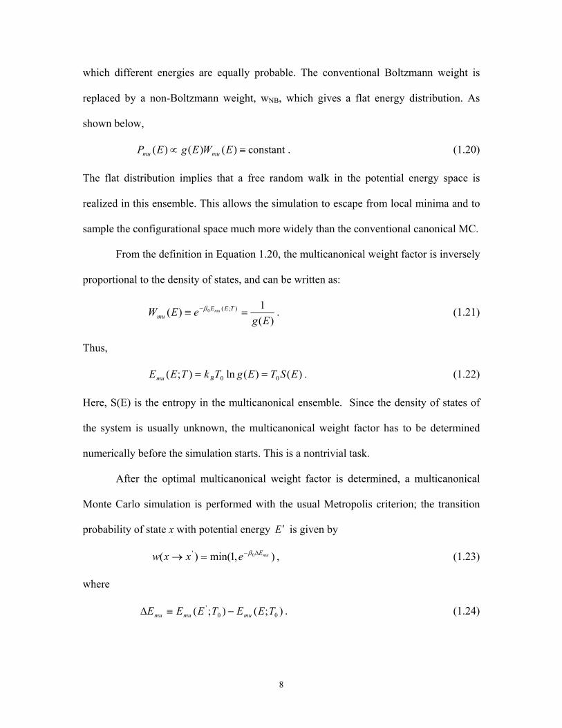
which different energies are equally probable. The conventional Boltzmann weight is
replaced by a non-Boltzmann weight, wNB, which gives a flat energy distribution. As
shown below,
≡∝ )()()( EWEgEP mumu constant . (1.20)
The flat distribution implies that a free random walk in the potential energy space is
realized in this ensemble. This allows the simulation to escape from local minima and to
sample the configurational space much more widely than the conventional canonical MC.
From the definition in Equation 1.20, the multicanonical weight factor is inversely
proportional to the density of states, and can be written as:
)(1)( );(0
EgeEW TEE
mumu =≡ −β . (1.21)
Thus,
)()(ln);( 00 ESTEgTkTEE Bmu == . (1.22)
Here, S(E) is the entropy in the multicanonical ensemble. Since the density of states of
the system is usually unknown, the multicanonical weight factor has to be determined
numerically before the simulation starts. This is a nontrivial task.
After the optimal multicanonical weight factor is determined, a multicanonical
Monte Carlo simulation is performed with the usual Metropolis criterion; the transition
probability of state x with potential energy E ′ is given by
),1min()( 0' muEexxw ∆−=→ β , (1.23)
where
);();( 00' TEETEEE mumumu −≡∆ . (1.24)
8

Once the estimate of the density of states is obtained, the multicanonical weight factor
can be directly determined by the formula below:
⎪⎪
⎩
⎪⎪
⎨
⎧
+−∂
∂=
+−∂
∂
=
=
=
);()();(
)(ln);(
);()();(
);(
00
00
00
0
TEEEEE
TEEEgkTTEE
TEEEEE
TEE
TEE
HmuHEEmu
mu
lmulEEmu
mu
H
l
(1.25)
where 1
1 TEE = , and
HTH EE = . The expectation value of a physical quantity A
at any temperature T is then calculated from
∑∑
−
−
=
E
EE
E
T eEg
eEgEAA β
β
)(
)()( (1.26)
It is a very difficult task to calculate density of states directly with high accuracy for large
systems. Almost all the methods to generate density of states are based on an
accumulation of the energy histogram. On the other hand, in a multicanonical simulation,
the density of states need not be very accurate. The re-weighting procedure does not
depend on the accuracy of the density of the states as long as the histogram can cover all
important energy levels with sufficient statistics.
1.4.3. Tsallis statistics
Tsallis statistics avoids the problem presented by the need to predetermine the
weight function in MUCA.25
The generalized thermostatistics proposed by Tsallis defines the generalized
entropy as
1
)(])(1[ 1
−
−=
−∫q
rprpdrkS
NTsallis
qNTsallis
N
Bq , (1.27)
9
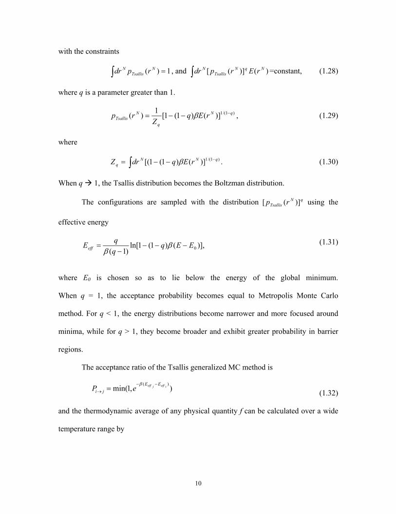
with the constraints
∫ = 1)( NTsallis
N rpdr , and ∫ )()]([ NqNTsallis
N rErpdr =constant, (1.28)
where q is a parameter greater than 1.
)1/(1)]()1(1[1)( qN
q
NTsallis rEq
Zrp −−−= β , (1.29)
where
)1/(1)]()1(1[( qNNq rEqdrZ −∫ −−= β . (1.30)
When q 1, the Tsallis distribution becomes the Boltzman distribution.
The configurations are sampled with the distribution using the
effective energy
qNTsallis rp )]([
(1.31) )],
((ln[ Eqq−−− β)11
)1( 0Eq
Eeff −=β
where E0 is chosen so as to lie below the energy of the global minimum.
When q = 1, the acceptance probability becomes equal to Metropolis Monte Carlo
method. For q < 1, the energy distributions become narrower and more focused around
minima, while for q > 1, they become broader and exhibit greater probability in barrier
regions.
The acceptance ratio of the Tsallis generalized MC method is
),1min()(
ieffjeff EEji eP
−−
→ =β
(1.32)
and the thermodynamic average of any physical quantity f can be calculated over a wide
temperature range by
10

∑∑
⋅
⋅⋅= −
−−
E
EE
E
T ew
ewff β
β
1
1
(1.33)
1.4.4. Wang-Landau free random walk in energy space
The free random walk in energy space with a flat histogram54,55 has become
known as “Wang-Landau sampling”. This algorithm is based on the observation that if
one performs a random walk in energy space and the probability to visit a given energy
level E is proportional to the reciprocal of the density of states 1/g(E), then a flat
histogram is generated for the energy distribution.
The partition function can be written as a sum over all states or over all energies
E,
∑∑ −− ==E
E
i
E eEgeZ i ββ )( , (1.34)
where g(E) is the density of states. Since g(E) is independent of temperature, it can be
used to find all properties of the system at different temperatures.
The idea of Wang-Laudau is very similar to multicanonical methods. An accurate
knowledge of the weight factors used in multicanonical methods is equivalent to a
knowledge of the density of states of the system. The Wang-Landau method directly and
self-consistently determines the density of states by performing a random walk in the
energy space, with a probability proportional to the reciprocal of the density of states. A
convertion factor is defined at the beginning of the simulation, starting with a big number
compared to 1. It will iteratively be updated when a flat energy histogram has been
achieved during the simulation. When the convertion factor is close to 1, a reliable and
accurate estimate of g(E) will be obtained.
1.4.5. Other methods
11
There are many more new sampling methods in Monte Carlo simulation besides
the four widely used algorithms described earlier. Hetenyi et al. introduced the multiple
“time step” Monte Carlo by divided the potential into a short- and long-range part56;
Berne et al. introduced catalytic Monte Carlo57; Brown et al. developed cool walking
algorithm58; and Transition Matrix Monte Carlo method59-61. Thus far, the most popular
methods using in sampling are parallel tempering Monte Carlo and multicanonical Monte
Carlo.
1.5. The overview of the thesis and application of advanced sampling algorithms
The thesis is mainly focused on using the advanced sampling method to
investigate weakly bound clusters. One of the reasons often stated for studying small
weakly bound clusters is that they provide a bridge between micro-systems and bulk
systems. Clusters can provide insights into the transformation from finite to bulk
behavior. They can also exhibit properties that are different from both the properties of
the individual atom or molecule and those of bulk matter.
In Chapter 2, the parallel tempering Monte Carlo procedure is applied to
investigate CO2 clusters. In spite of the importance of CO2 as a solvent, relatively little is
known about CO2 clusters. Exceptions are the CO2 dimer and trimer which have been the
subject of several experimental and theoretical studies. We are especially intrigued by the
thermodynamic properties, in particular the melting behavior, of CO2 clusters and how
this behavior depends on the details of the underlying potential energy surface.
In Chapter 3, a hybrid algorithm of parallel tempering Monte Carlo simulation
and Tsallis statistics has been introduced and applied on a 1D model potential. The LJ38
cluster, which is known to have an extremely rugged potential energy surface has been
12
investigate using both parallel tempering Monte Carlo and the hybrid algorithm. The
results show the when the simulation starting from the second minima, the simulations
tend to very hard to reach equilibrium and it shows the potential to be a very good test
system for new algorithm development. Comparing to PTMC, the hybrid algorithm is
about 10 times faster for reaching equilibrium in the 1D model potential and is about 3
times faster for reaching equilibrium in the Ar38 system when starting from the second
lowest energy minimum.
In Chapter 4, the Wang-Landau free random walk algorithm is used in simulation
of Ar13 and Ar38. The algorithm is found to work well for Ar13 which has a simple
potential energy landscape. However, in the Ar38 system, difficulties are met in reaching
a flat distribution because of the difficulty in generating configurations in the low-energy
regions.
Appendix A is a separated project collaborated with professor Cohen. The
research is focused on computational study of the stereochemistry of intramolecular
carbolithiation of a secondary alkyllithium to produce a 2-substituted
cyclopentylmethyllithium using DFT theory.
Appendix B is a project that I have involved. My major contribution for that
project is using eigenmode following algorithm to locate the global minima of (H2O)21.
,
13
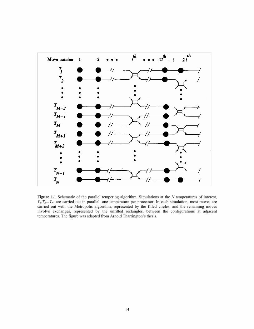
Figure 1.1 Schematic of the parallel tempering algorithm. Simulations at the N temperatures of interest, T1,T2…TN are carried out in parallel, one temperature per processor. In each simulation, most moves are carried out with the Metropolis algorithm, represented by the filled circles, and the remaining moves involve exchanges, represented by the unfilled rectangles, between the configurations at adjacent temperatures. The figure was adapted from Arnold Tharrington’s thesis.
14
2. Chapter 2 Finite temperature properties of (CO2)n clusters
2.1. Introduction
Carbon dioxide has attracted considerable experimental and theoretical attention
both because of the importance of its supercritical state for chemical separations and
because it is a prototype for molecules for which the dominant electrostatic interactions
are quadrupole-quadrupole in nature.62 Although the net dipole moment for CO2 is zero,
there is a clear charge separation in CO2 molecule with the bond electron density being
polarized more towards the oxygen atoms, leaving the carbon atom with a partial positive
charge and the two oxygen atoms with partial negative charges. Because the molecular
charge is very well characterized, CO2 has attracted attention from the theorists. For
example, the crystal structure, volume compression and vibrational properties of solid
CO2 have been calculated with various model potentials and compared with the
experimental results.63-65
In spite of this, our knowledge of the properties of CO2 clusters lags behind that
for clusters of polar molecules such as water. Although several Monte Carlo and
molecular dynamic simulations of (CO2)n clusters have been carried out,66-70 there remain
unresolved issues including the connections between the thermodynamic behavior and
the topology of the underlying potential energy surfaces. Also, it appears that some of
these simulations failed to achieve equilibrium, particularly at the lowest temperatures
considered.
In the present study the parallel-tempering Monte Carlo method,71 which is well
suited for achieving equilibrium in low-temperature simulations when there are large
energy barriers separating low-lying local potential energy minima, is combined with
long production cycles to calculate the finite-temperature behavior of (CO2)n, n = 6, 8, 13,
15
and 19, clusters. To aid in analyzing the nature of the transitions associated with peaks in
the heat capacity curves, the populations of inherent structures are calculated as a
function of temperature. Stillinger and Weber proposed the idea to partitioning the
potential surface into basins of attractions72. The inherent structures of quenching provide
insight into the accessible local minima of the potential energy surface for a temperature
of simulation. Later, Becker and Karplus introduced disconnecitivity diagrams to
represent the topology of the potential energy surface73. Those two methods are
combined in our analysis to help describe the potential energy surface. For each
simulation, the saved configurations are quenched (minimized) to their closed local
minimum. For each cluster considered, the low-energy minima and transition states are
located using the eigenmode-following method74-76 and used to construct disconnectivity
graphs to provide insight into the topology of the potential energy surface, in particular,
the accessibility of different regions of configuration space as a function of energy.
Simulations of (CO2)38 are also performed using parallel tempering Monte Carlo method.
2.2.Methodology
2.2.1. Model potential
The CO2 - CO2 interactions are described by a two-body model potential due to
Murthy et al.77 This is a rigid monomer model with CO bond lengths equal to the
experimental (Re) value and interactions between monomers described by electrostatic
and 6-12 Lennard-Jones terms. The former are incorporated by means of five point
charges on each monomer, the locations and values of which are given in Table 1. The
Lennard - Jones terms are atom-atom in nature, with the parameters being given in Table
2.
16
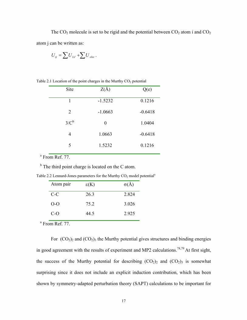
The CO2 molecule is set to be rigid and the potential between CO2 atom i and CO2
atom j can be written as:
elecLJij UUU ∑∑ += .
Table 2.1 Location of the point charges in the Murthy CO2 potential
Site Z(Å) Q(e)
1 -1.5232 0.1216
2 -1.0663 -0.6418
3/Cb 0 1.0404
4 1.0663 -0.6418
5 1.5232 0.1216
a From Ref. 77. b The third point charge is located on the C atom.
Table 2.2 Lennard-Jones parameters for the Murthy CO2 model potentiala
Atom pair ε(K) σ(Å)
C-C 26.3 2.824
O-O 75.2 3.026
C-O 44.5 2.925
a From Ref. 77.
For (CO2)2 and (CO2)3 the Murthy potential gives structures and binding energies
in good agreement with the results of experiment and MP2 calculations.78,79 At first sight,
the success of the Murthy potential for describing (CO2)2 and (CO2)3 is somewhat
surprising since it does not include an explicit induction contribution, which has been
shown by symmetry-adapted perturbation theory (SAPT) calculations to be important for
17
these clusters.80 This suggests that either the LJ or the electrostatic term (or perhaps both)
in the Murthy potential is too attractive, thereby “mimicking” the induction interactions.
The use of enhanced electrostatic terms to incorporate induction is a common procedure,
with a representative example being the TIP4P model for water.81
2.2.2. Parallel tempering Monte Carlo procedure
Monte Carlo simulations were carried out using the parallel tempering
algorithm,34,35 in which simulations over the range of temperatures of interest are carried
out in parallel. The sets of configurations generated at the various temperatures are called
“replicas”. Most moves are “local”, i.e., confined to individual replicas, with trial moves
translations or rotations of individual molecules, being accepted or rejected according to
the Metropolis algorithm:
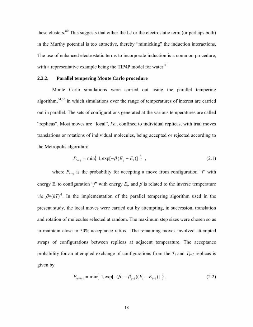
{ )](exp[,1min ijji EEP }−−=→ β , (2.1)
where Pi→j is the probability for accepting a move from configuration “i” with
energy Ei to configuration “j” with energy Ej, and β is related to the inverse temperature
via β=(kT)-1. In the implementation of the parallel tempering algorithm used in the
present study, the local moves were carried out by attempting, in succession, translation
and rotation of molecules selected at random. The maximum step sizes were chosen so as
to maintain close to 50% acceptance ratios. The remaining moves involved attempted
swaps of configurations between replicas at adjacent temperature. The acceptance
probability for an attempted exchange of configurations from the Ti and Ti+1 replicas is
given by
{ })])((exp[,1min 111 +++↔ −−−= iiiiii EEP ββ , (2.2)
18
where βi = (kTi)-1. Exchanges were attempted once every 100 moves, and were
made only between replicas at adjacent temperatures. On odd swap cycles, the attempted
exchanges were between the (T1, T2), (T3, T4), etc. replicas, and on even cycles, between
the (T2, T3), (T4, T5), etc. replicas. Additional details on the parallel tempering code used
to carry out the simulations are given in Ref. 82.
At the highest temperatures used in the simulations, evaporative events could
occur, which would seriously impact convergence. This problem was avoided in the
simulations on the three smaller clusters by rejecting moves that placed one or more of
the molecules over a specified distance [6 Å for (CO2)6 and (CO2)8 and 8 Å for (CO2)13 ]
from the center of mass of the cluster. For (CO2)19, moves that placed the C atom of an
individual monomer more than 5 Å from the C atoms of all other monomers in the cluster
were rejected. This constraint method is called “maximum group distance” method. The
difference constraint method for (CO2)19 cluster allows the cluster having extended forms
as well as compact forms.
One of the challenges in carrying out parallel-tempering Monte Carlo simulations
is the choice of an appropriate grid of temperatures covering the temperature range of
interest. The temperature range should encompass regions over which the structural
transformations of interest occur. It is also essential that all important energy barriers are
readily overcome at the highest temperature employed and that there is appreciable
overlap between the potential energy distributions from the simulations at adjacent
temperatures. In the present study, twenty temperatures spanning 20-150 K were used for
(CO2)n, n = 6, 8, 13, and twenty-four temperatures spanning 20-200 K were used for
(CO2)19. These temperature ranges were chosen on the basis of series of preliminary
19
parallel-tempering Monte Carlo simulations with different choices of the temperatures.
Additional simulations, employing up to 28 temperatures, were also carried out, results
obtained were very close to those from the simulations using fewer temperatures.
For each cluster studied, two parallel-tempering Monte Carlo simulations were
carried out, one starting from a configuration chosen at random from a preliminary high-
temperature Metropolis Monte-Carlo simulation, and the other starting from the global
minimum structure. Comparison of the results of the two simulations provides a check
on attainment of equilibrium. For each simulation, averaging was done over 2×10⁷
moves following an equilibration period, which ranged from 107 moves for (CO2)6 and
(CO2)8 to 2×10⁷ moves for (CO2)13 and 3× 10⁷ moves for (CO2)19. The equilibration data
are not counted on the average. Each standard Monte Carlo move includes a translation
move of a random picked molecule and a rotational move a random picked molecule. The
step size of each kind of moved are adjusted every 1000 moves in the equilibration
period. The acceptance criterion for the translational and rotational moves was
maintained 50% by adjusting the step size. During the simulation, the configurations are
saved every 40000 moves for further analysis.
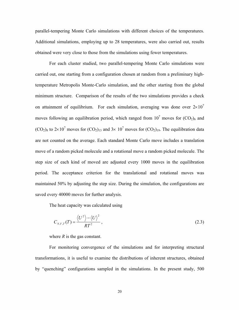
The heat capacity was calculated using
2
22
,, )(RT
UUTC TVN
−= , (2.3)
where R is the gas constant.
For monitoring convergence of the simulations and for interpreting structural
transformations, it is useful to examine the distributions of inherent structures, obtained
by “quenching” configurations sampled in the simulations. In the present study, 500
20
configurations, chosen at equal intervals, were saved from each replica and optimized to
their inherent structures by use of the eigenmode-following method as implemented in
the Orient 4.3 program.83
2.2.3. Disconnectivity graphs
Over the past few years much progress has been made in establishing the
relationship between the topology of the potential energy surface and the difficulty of
achieving equilibrium in finite temperature (or energy) simulations.82,84,85 This requires
locating the local potential energy minima and the transition states connecting the
minima. In the present study, this was accomplished by carrying out eigenmode-
following (EF)74,76 searches in directions, both parallel and anti-parallel to specific
eigenvectors of the Hessian, for each of the minima located in the course of the
optimizations. Searches were done along the eigenvector associated with the lowest 8, 15,
24 and 50 eigenvalues for (CO2)6, (CO2)8, (CO2)13 and (CO2)19, respectively. For each
transition state located in this manner, subsequent searches were carried out to identify
the minima connected to the transition state, allowing construction of the rearrangement
pathways. These results were used to construct disconnectivity graphs,86 which show the
minima that are accessible at different energy thresholds and thus provide a convenient
visual representation of the connectivity/disconnectivity of different regions of the
potential energy surface.73,86
2.3. Results
The heat capacity vs. temperature curves, obtained from the parallel-tempering
simulations, are shown in Figure 2.1. For each cluster, curves from both the simulation
started at the global minimum structure and that started from a randomly selected
21
structure are reported and found to be in excellent agreement, providing evidence that the
calculations have achieved equilibrium. The heat capacity curves of (CO2)6 and (CO2)8
display broad, weak peaks centered near T = 70 K. In contrast, the heat capacity curves of
(CO2)13 and (CO2)19 display pronounced, narrower peaks near T = 90 K. In analyzing
these results, it is useful to examine the low-energy minima from the EF optimizations,
the distributions of inherent structures sampled in the finite temperature simulations, and
the disconnectivity graphs. The energies of the low-lying local minima of the various
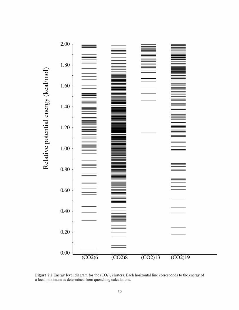
clusters are indicated in Figure 2.2. The analyses of the results for various clusters are
presented below.
i) (CO2)6
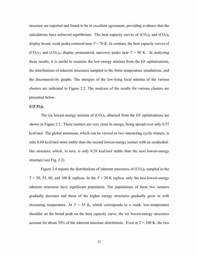
The six lowest-energy minima of (CO2)6 obtained from the EF optimizations are
shown in Figure 2.3. These isomers are very close in energy, being spread over only 0.57
kcal/mol. The global minimum, which can be viewed as two interacting cyclic trimers, is
only 0.04 kcal/mol more stable than the second lowest-energy isomer with an octahedral-
like structure, which, in turn, is only 0.28 kcal/mol stable than the next lowest-energy
structure (see Fig. 2.2).
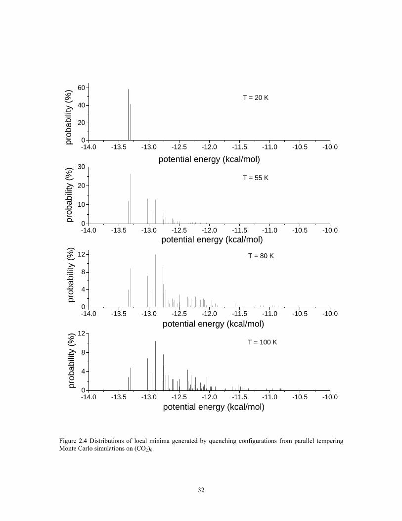
Figure 2.4 reports the distributions of inherent structures of (CO2)6 sampled in the
T = 20, 55, 80, and 100 K replicas. In the T = 20 K replica, only the two lowest-energy
inherent structures have significant population. The populations of these two isomers
gradually decrease and those of the higher energy structures gradually grow in with
increasing temperature. At T = 55 K, which corresponds to a weak, low-temperature
shoulder on the broad peak on the heat capacity curve, the six lowest-energy structures
account for about 70% of the inherent structure distribution. Even at T = 100 K, the two
22
lowest-energy structures together still account for about 9% of the population and the six
lowest-energy structures for about 32% of the population. Although Etters et al.2
concluded that (CO2)6 undergoes a melting transition near 70 K, in our opinion, the
density of states near this temperature is not sufficiently high to attribute the broad, weak
peak in the heat capacity curve to a melting transition.
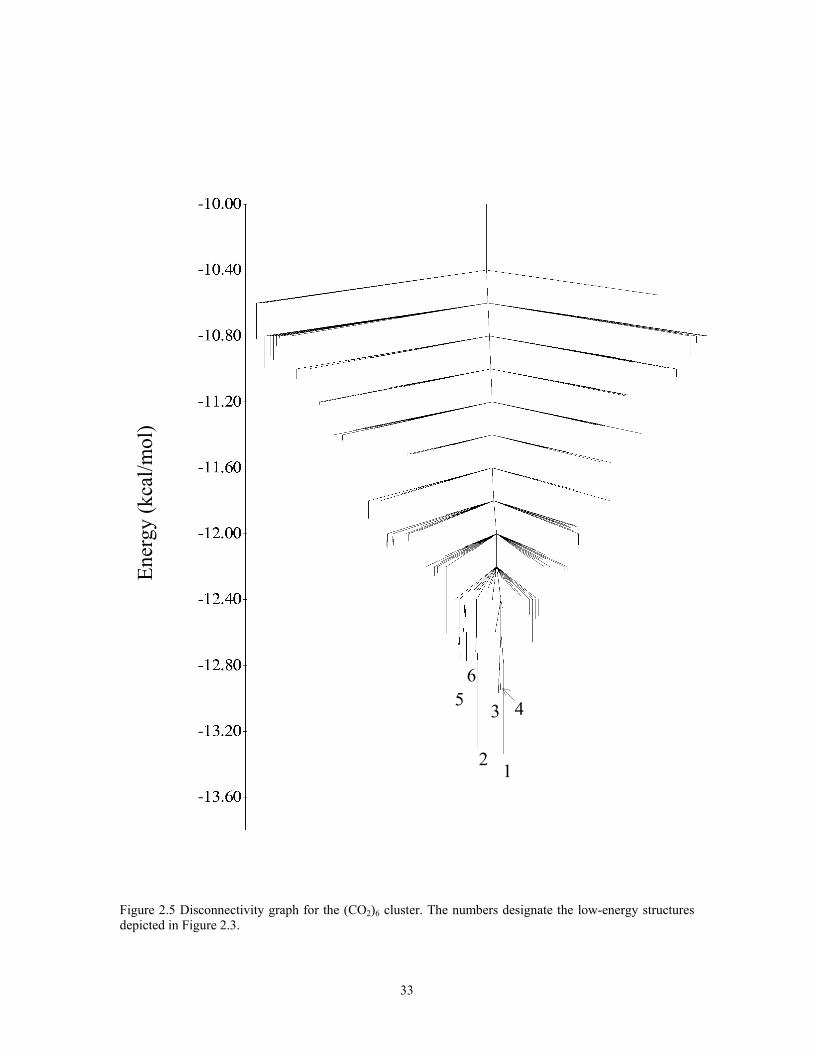
The disconnectivity graph for (CO2)6 is shown in Figure 2.5. Overall, the diagram
is quite simple, and the potential energy surface can be characterized as having a single
funnel. There is a barrier of about 1 kcal/mol for interconversion of the two lowest energy
isomers. Thus, it should be possible to achieve sizable populations of both these isomers
in a seeded expansion.
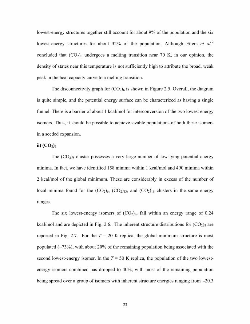
ii) (CO2)8
The (CO2)8 cluster possesses a very large number of low-lying potential energy
minima. In fact, we have identified 158 minima within 1 kcal/mol and 490 minima within
2 kcal/mol of the global minimum. These are considerably in excess of the number of
local minima found for the (CO2)6, (CO2)13, and (CO2)19 clusters in the same energy
ranges.
The six lowest-energy isomers of (CO2)8, fall within an energy range of 0.24
kcal/mol and are depicted in Fig. 2.6. The inherent structure distributions for (CO2)8 are
reported in Fig. 2.7. For the T = 20 K replica, the global minimum structure is most
populated (~73%), with about 20% of the remaining population being associated with the
second lowest-energy isomer. In the T = 50 K replica, the population of the two lowest-
energy isomers combined has dropped to 40%, with most of the remaining population
being spread over a group of isomers with inherent structure energies ranging from -20.3
23

to -19.8 kcal/mol. In the T = 80 K replica, the net population of the two lowest-energy
isomers has dropped to about 7%, with the remaining population being spread over a
large number of isomers.
The disconnectivity graph for (CO2)8 is shown in Fig. 2.8. The potential energy
surface of this cluster is characterized by two low-energy basins, each containing about
20 local minima. There is a barrier of about 1 kcal/mol between the lowest-energy
structures in one basin to the lowest-energy structure in the other basin. Comparison of
Figures 2.7 and 2.8 reveals that near T = 70 K the (CO2)8 cluster has an appreciable
population of higher-energy structures associated with the two low-energy basins as well
as of a large number of structures associated with other regions of the potential energy
surface. While, the density of inherent structures is high enough to view the cluster as
“liquid-like” for temperatures above about 80 K, this system does not possess a sizable
energy gap between the global minimum or small group of low-energy minima and the
remaining higher-lying minima (see Fig. 2.2), and it has been argued that such an energy
gap is required for a cluster to display a well-defined melting transition.87 Due to the
absence of the energy gap, the broad transition found for (CO2)8 can be viewed as “glass-
like” rather than originating from a well-defined melting transition.
iii) (CO2)13
The structures of the six lowest-energy isomers of the (CO2)13 cluster are shown
in Fig. 2.9. In agreement with Ref. 69, the global minimum has an icosahedral-like
structure of S6 symmetry. The global minimum is predicted to be 1.16 kcal/mol more
stable than the second lowest-energy isomer, which belongs to a group of isomers with
distorted icosahedral structures. This situation is analogous to that for the LJ13 cluster, for
24
which the global minimum is a highly stable icosahedral structure, followed in energy by
a group of distorted-icosahedral isomers, and then by non-icosahedral structures.88
The inherent structure distributions of (CO2)13 are reported in Fig. 2.10. Only the
global minimum structure has an appreciable population in the T = 20 K replica. Even at
T = 60 K, it accounts for over 99% of the total population. However, at T = 90 K, the
population of the global minimum structure has dropped to about 48%, with the
remaining population being spread over a large number of higher-energy structures. At T
= 110 K, the population of the global minimum structure has fallen to below 0.5%.
The inherent structure distributions and the large peak in the heat capacity curve
of (CO2)13 are both indicative of a relatively sharp melting transition near 90 K. This is in
agreement with Maillet et al., who concluded on the basis of molecular dynamics
simulations that the (CO2)13 cluster melts near T = 95 K. The disconnectivity graph for
(CO2)13 shown in Fig. 2.11 displays a single-funnel topology similar to that found for
LJ13.
iv) (CO2)19
The geometries of the six lowest-energy isomers of (CO2)19 are shown in figure
2.12. All of these may be viewed as icosahedral-like with an approximately icosahedal
(CO2)13 core and with the remaining six molecules forming a surface layer. These six
isomers are close in energy, being spread over only 0.5 kcal/mol. The inherent structure
distributions are plotted in figure 2.13. For the T = 20 K replica, about 87% of the
population is associated with the global minimum, with the remaining population being
due to the next two-lowest energy isomers. At T = 50 K, these three isomers still
dominate, but now isomer 2, is most populated at 38%. At T = 80 K, somewhat below the
25

temperature of the maximum in the large peak in the heat capacity curve, the net
population of the three lowest energy isomers has fallen to about 8%, with the remaining
population being distributed over a large number of higher-lying isomers. At T = 100 K,
there is no significant population of the six lowest-energy isomers. The trends in the
inherent structure distributions provide strong evidence that the large peak near 90 K in
the heat capacity curve of (CO2)19 is due to a melting-like transition. This is consistent
with the conclusion of Maillet et al., who reported, based on molecular dynamics
simulations, that (CO2)19 melts near T = 95 K.
The heat capacity curve for (CO2)19 also displays a weak shoulder near T = 50 K.
This is due to a “solid” to “solid” transition between isomer 1 and isomers 2 and 3. This
interpretation is supported by the disconnectivity graph of (CO2)19 shown in Fig. 14,
which reveals that each of the three low-energy isomers is associated with a different
basin. The barriers to go from the lowest-energy isomer to the basins containing isomers
2 and 3 are over 3 kcal/mol.
As we have mentioned before, the simulations of (CO2)19 were also carried out at
28 temperature replicas for comparation the convergence of the simulations and
investigation of the influence of temperature spacing. 28 temperatures ranging from 20 –
150 K have been applied to the simulation. The temperature grids for those extra
simulations are finer. Figure 2.15 shows the results of heat capacity curves running at
different temperature grids. From Figure 2.15 we can see there is no distinguishable
difference among the results of simulations with different temperature grids. The
simulation using 24 temperatures spanning from 20 – 200 K is good and have enough
overlap between the sampling distributions.
26
v) (CO2)38
The parallel tempering Monte Carlo algorithms are also applied to the simulation
of (CO2)38 cluster. Two runs of simulations have been performed with different random
start geometry and slightly different temperature spacings. 32 temperatures has been used
from 20K to 200K. The heat capacity results are reported in figure 2.16. For each
simulation, the average results are calculated over the production cycle of 4x10⁷ cycles,
which following by the equilibrium cycles is around 4x10⁷ steps. Similar to the
simulations of (CO2)19, the constraint method to prevent evaporation is so called
“maximum group distance” method. Moves that placed the C atom of an individual
monomer more than 8 Å from the C atoms of all other monomers in the cluster were
rejected. It appears that the system has not reach equilibrium since the agreements in the
heat capacity curves between the two runs are not very well. But both of them show the
similar pattern with two peaks in the heat capacity curves. There is a broad peak around
100 K and an extra sharp big peak around 180 K. The broad peak about 100 K may be
described as a solid-solid state transition. The sharp peak around 180 K may be described
as the melting transition. The temperature of the sharp peak is in a fair good agreement
with the sublimation temperature of dry ice which is 194.5 K.
2.4. Conclusions
In this paper the finite temperature behavior of the (CO2)n, n = 6, 8, 13, and 19,
clusters has been investigated by means of parallel-tempering Monte Carlo simulations.
The results have been analyzed in terms of inherent structure distributions and
disconnectivity graphs. The question of when to characterize a structural transformation
in a small cluster as a melting transition has been the subject of much discussion in the
27
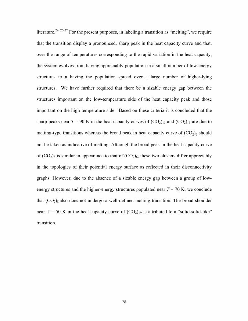
literature.24, 26-27 For the present purposes, in labeling a transition as “melting”, we require
that the transition display a pronounced, sharp peak in the heat capacity curve and that,
over the range of temperatures corresponding to the rapid variation in the heat capacity,
the system evolves from having appreciably population in a small number of low-energy
structures to a having the population spread over a large number of higher-lying
structures. We have further required that there be a sizable energy gap between the
structures important on the low-temperature side of the heat capacity peak and those
important on the high temperature side. Based on these criteria it is concluded that the
sharp peaks near T = 90 K in the heat capacity curves of (CO2)13 and (CO2)19 are due to
melting-type transitions whereas the broad peak in heat capacity curve of (CO2)6 should
not be taken as indicative of melting. Although the broad peak in the heat capacity curve
of (CO2)8 is similar in appearance to that of (CO2)6, these two clusters differ appreciably
in the topologies of their potential energy surface as reflected in their disconnectivity
graphs. However, due to the absence of a sizable energy gap between a group of low-
energy structures and the higher-energy structures populated near T = 70 K, we conclude
that (CO2)8 also does not undergo a well-defined melting transition. The broad shoulder
near T = 50 K in the heat capacity curve of (CO2)19 is attributed to a “solid-solid-like”
transition.
28

0
5
10
15
20
25
30
35
40
45
0 50 100 150 200
Temperature (K)
Cv
(cal
/mol
-K)
CO2_6_run1CO2_6_run2CO2_8_run1CO2_8_run2CO2_13_run1CO2_13_run2CO2_19_run1CO2_19_run2
Figure 2.1 Heat capacity curves of the (CO2)n clusters calculated by means of parallel tempering Monte Carlo simulations. For each cluster, run1 denotes the simulation starting from global minimum and run2 denotes the simulation starting from a random geometry.
29
Rel
ativ
e po
tent
ial e
nerg
y (k
cal/m
ol)
Figure 2.2 Energy level diagram for the (CO2)n clusters. Each horizontal line corresponds to the energy of a local minimum as determined from quenching calculations.
30

nima of (CO2)6
Figure 2.3 Structures of the six lowest-energy mi fro
(1) -13.34 kcal/mol
(5) -12.89 kcal/mol
31
PE=-13.30kcal/mol(2) -13.30 kcal/
(3) -13.02 kcal/molm ei
(4) -12.95 kcal/mol
(6) -12.77 kcal/molmol
genmode-following optimizations.
-14.0 -13.5 -13.0 -12.5 -12.0 -11.5 -11.0 -10.5 -10.00
20
40
60
prob
abilit
y (%
)pr
obab
ility
(%)
potential energy (kcal/mol)
potential energy (kcal/mol)
prob
abilit
y (%
)
potential energy (kcal/mol)
T = 20 K
prob
abilit
y (%
)
potential energy (kcal/mol)
-14.0 -13.5 -13.0 -12.5 -12.0 -11.5 -11.0 -10.5 -10.00
10
20
30T = 55 K
-14.0 -13.5 -13.0 -12.5 -12.0 -11.5 -11.0 -10.5 -10.00
4
8
12 T = 80 K
-14.0 -13.5 -13.0 -12.5 -12.0 -11.5 -11.0 -10.5 -10.00
4
8
12T = 100 K
Figure 2.4 Distributions of local minima generated by quenching configurations from parallel tempering Monte Carlo simulations on (CO2)6.
32
12
3 456
Ener
gy (k
cal/m
ol)
igure 2.5 Disconnectivity graph for the (CO2)6 cluster. The numbers designate the low-energy structures F
depicted in Figure 2.3.
33
Figu
(1) -20.29 kcal/mol
re 2.6 Structures of the six lowest-energy minima of (CO2)8 from eig
34
0
(2) -2 .23 kcal/mol (3) -20.21 kcal/mol(4) -20.12 kcal/mol
(5) -20.09 kcal/mol (6) -20.05 kcal/molenmode-following optimizations.
-21.0 -20.5 -20.0 -19.5 -19.0 -18.5 -18.0 -17.5 -17.0 -16.5 -16.00
20
40
60
80
prob
abilit
y (%
)pr
obab
ility
(%)
prob
abilit
y (%
)
potential energy (kcal/mol)
potential energy (kcal/mol)
T = 20 K
prob
abilit
y (%
)
potential energy (kcal/mol)
-21.0 -20.5 -20.0 -19.5 -19.0 -18.5 -18.0 -17.5 -17.0 -16.5 -16.00
10
20
30 T = 50 K
-21.0 -20.5 -20.0 -19.5 -19.0 -18.5 -18.0 -17.5 -17.0 -16.5 -16.00
1
2
3
4
5T = 80 K
-21.0 -20.5 -20.0 -19.5 -19.0 -18.5 -18.0 -17.5 -17.0 -16.5 -16.00
1
2 T = 100 K
potential energy (kcal/mol)
Figure 2.7 Distributions of local minima generated by quenching configurations from parallel tempering Monte Carlo simulations on (CO2)8.
35
12
34
56
Ener
gy (k
cal/m
ol)
Figure 2.8 Disconnectivity graph for the (CO2)8 cluster. The numbers designate the low-energy structures depicted in Figure 2.6.
36
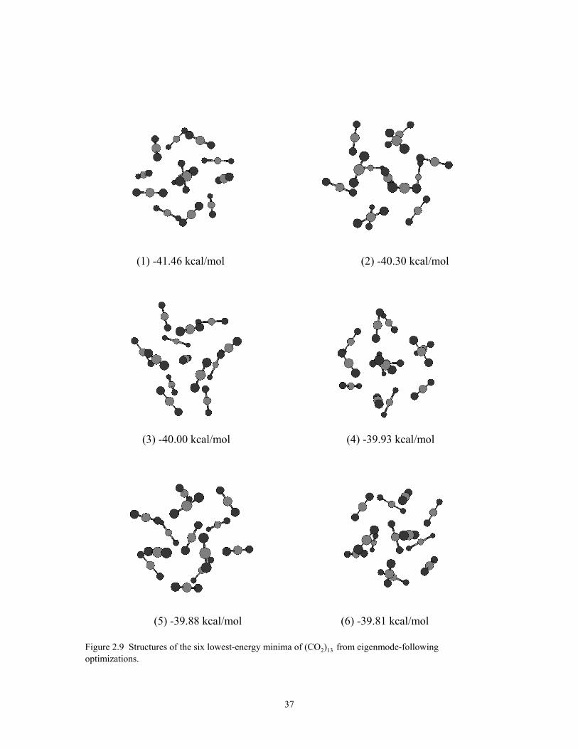
Figure 2optimiz
(1) PE=-41.46 kcal/mol
.9 Structures of the six lowest-energy minima of (CO2)13 from ations.
37
(2) -40.30 kcal/mol
(1) -41.46 kcal/mol (3) -40.00 kcal/mol (4) -39.93 kcal/mol (5) -39.88 kcal/mol (6) -39.81 kcal/moleigenmode-following

-42 -41 -40 -39 -38 -37 -36 -35 -34 -33 -32 -31 -300
20
40
60
80
100
prob
abilit
y (%
)pr
obab
ility
(%)
prob
abilit
y (%
)T = 20 K
prob
abilit
y (%
)
potential energy (kcal/mol)
-42 -410.0
0.2
0.4
0.6
0.8
1.0T = 60 K
-42 -410.0
0.2
0.4
0.6
0.8
1.0
-42 -410.0
0.4
0.8
1.2
1.6
×
×0.0
Figure 2.10 Distributions oMonte Carlo simulations o
0.01
potential energy (kcal/mol)
potential energy (kcal/mol)-40 -39 -38 -37 -36 -35 -34 -33 -32 -31 -30
-40 -39 -38 -37 -36 -35 -34 -33 -32 -31 -30
T = 90 K
-40 -39 -38 -37 -36 -35 -34 -33 -32 -31 -30
potential energy (kcal/mol)
T = 110 K
1
f local minima generated by quenching configurations from parallel tempering n (CO2)13.
38
1
2345 6
Ener
gy (k
cal/m
ol)
Figure 2.11 Disconnectivity graph for the (CO2)13 cluster. The numbers designate the low-energy structures depicted in Figure 2.9.
39
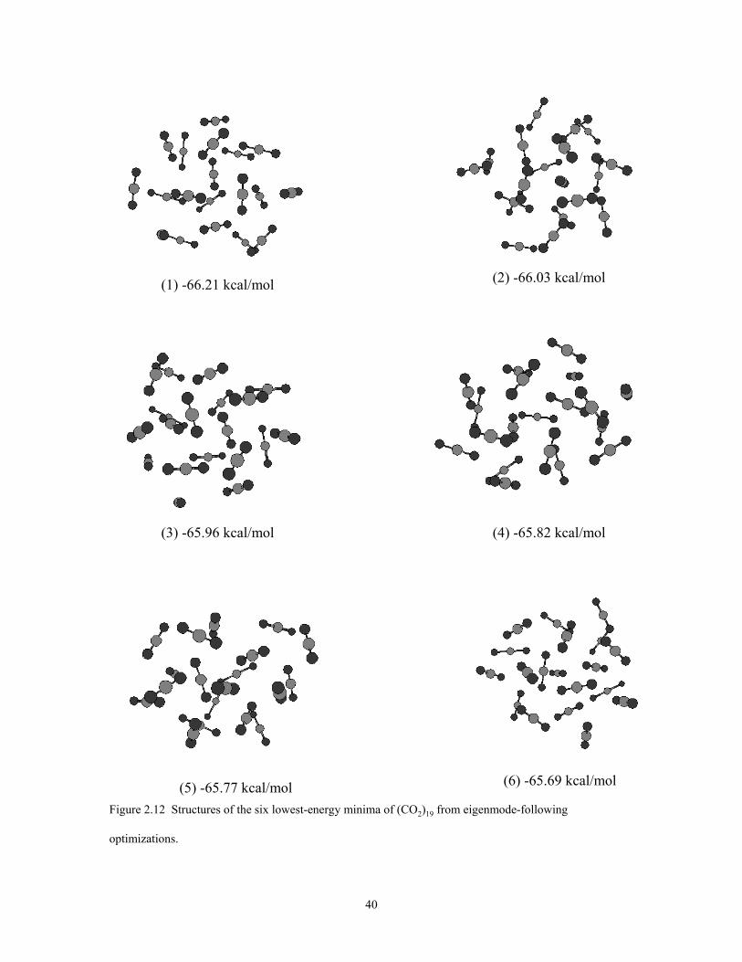
Figure 2.1
optimizat
(1) -66.21 kcal/mol
2 Structures of the six lowest-energy minima of (CO2)19 from eigen
ions.
40
(2) -66.03 kcal/mol
(3) -65.96 kcal/mol (4) -65.82 kcal/mol (5) -65.77 kcal/mol m(6) -65.69 kcal/mol
ode-following
-66 -64 -62 -60 -58 -560
10
20
30
40
T = 50 K
prob
abilit
y (%
)pr
obab
ility
(%)
prob
abilit
y (%
)pr
obab
ility
(%)
prob
abilit
y (%
)
potential energy (kcal/mol)
potential energy (kcal/mol)
potential energy (kcal/mol)
potential energy (kcal/mol)
-66 -64 -62 -60 -58 -560
20
40
60
80
T = 20 K
-66 -64 -62 -60 -58 -560
2
4
6
T = 80 K
-66 -64 -62 -60 -58 -560
1
2
T = 90 K
-66 -64 -62 -60 -58 -560.0
0.4
0.8
1.2T = 110 K
potential energy (kcal/mol)
Figure 2.13 Distributions of local minima generated by quenching configurations from parallel tempering Monte Carlo simulations on (CO2)19.
41

1 2 345 6
Ener
gy (k
cal/m
ol)
Figure 2.14 Disconnectivity graph for the (CO2)19 cluster. The numbers designate the low-energy structures depicted in Figure 2.12.
42
0
5
10
15
20
25
30
0 50 100 150 200
Temperature
Cv/
(cal
/mol
-K)
run2
run3
run1
Figure 2.15 Heat capacity curves of (CO2)19 calculated by means of parallel tempering Monte Carlo simulations. The run 1 denotes the simulations carried out with 24 temperatures spanning from 20 – 200 K, which is the same figure reported in Figure 2.1; run 2 denotes the simulation carried out with 28 temperatures spanning from 20 – 150 K; run 3 denotes the simulation carried out with the same temperature grid as run 2, but starting from a random geometry.
43
0
20
40
60
80
100
120
0 50 100 150 200 250
Temperature
Cv
/(cal
/mol
-K)
(CO2)38 run1 (CO2)38 run2
Figure 2.16 Heat capacity curves of (CO2)38 calculated by means of parallel tempering Monte Carlo simulation. Run1 and run2 denote simulations starting from different randomly picked starting geometries.
44
3. Chapter 3 On the Convergence of Parallel Tempering Monte Carlo Simulations of LJ38
3.1. Introduction
The conventional Metropolis algorithm for sampling the canonical distribution
has difficulties dealing with the problem of quasi-ergodicity associated with complex
potential energy landscapes. Recently, considerable progress has been made in
developing efficient sampling algorithms for dealing with this problem. The parallel
tempering algorithm has been used extensively as a means of improving sampling.
However, it suffers from the need to use an increasing number of temperatures with
increasing system size. The details of the parallel tempering algorithm were given in
Chapters 1 and 2.
This chapter, describes an effective hybrid scheme for combining parallel
tempering Monte Carlo and Tsallis generalized statistics. As mentioned in Chapter 1,
Tsallis statistics employ more delocalized potential energy distributions than does
sampling from the Boltzman distribution. Thus, the hybrid scheme might be expected to
give improved convergence. The strategy is similar in spirit to work of Sugita et al., who
introduced a parallel tempering multicanonical algorithm89,90. Whitfield et al91. and Jang
et al92. have previously combined parallel tempering with Tsallis statistics. In both their
approaches, each replica at a specified target temperature is run with different q values.
Exchanges of configurations are allowed between simulations with different q values but
at the same T. Our hybrid scheme is an extension of the original parallel tempering Monte
Carlo, with sampling being done in the Tsallis generalized ensemble at different
temperatures, and the exchange of configurations between different replicas
45
(temperatures) being permitted. Results for the canonical ensemble are obtained by using
the histogram reweighting to transform between ensembles.
Four different approaches – parallel tempering Tsallis statistics, parallel
tempering Monte Carlo, Metropolis Monte Carlo, and Tsallis statistics based Monte
Carlo - are applied to a 1D model potential and to the LJ38 cluster.
The 38-atom Lennard Jones (LJ38) cluster has a global minimum with an Oh
symmetry FCC-like structure followed by a C5v symmetry icosahedral isomer lying only
slightly higher in energy, see figure 3.2. These two minima are separated by a
complicated rearrangement pathway with a high overall barrier. The funnel leading to the
C5v potential energy minimum is much broader than that leading to the FCC minimum,85
and, as a result, it is difficult to locate the global minimum starting from an arbitrary
structure and to achieve equilibrium in low temperature Monte Carlo simulations. For
these reasons the LJ38 cluster has proven to be a valuable system for testing global
optimization and Monte Carlo simulation algorithms.71,93-95 Figure 3.1 shows the
disconnectivity diagram of LJ38.74 This diagram helps convery a sense of the complexity
of the potential energy surface of LJ38.
The LJ38 cluster, with parameters appropriate for Ar, and referred to here as Ar38,
has been employed by Neirotti et al.,71 Calvo et al.,94 and Frantz29 to demonstrate the
utility of parallel-tempering Monte Carlo (PTMC) procedure34,96-98 for achieving
equilibrium in systems prone to quasiergodic behavior. The heat capacity curve of Ar38 as
treated classically has a pronounced peak near T = 20 K due to cluster melting and a
weak shoulder near T = 15 K due to the FCC icosahedral transition. Traditional Monte
Carlo simulations with Metropolis sampling6 are unable to properly characterize the Ar38
46

cluster at temperatures in the vicinity of the latter transition. Neirotti et al. were able to
overcome this problem by use the PTMC procedure in which Monte Carlo simulations
are carried out for a range of temperatures and exchanges of configurations between
different temperature simulations (replicas) are permitted. The PTMC simulations of
Neirotti et al. employed 32 temperatures (from 0.5 to 30 K), an equilibration period of
2.85x10⁸ moves, and production cycles of 1.3x10¹⁰ moves at each temperature. Most
moves for each replica were carried out using the Metropolis algorithm. An exchange of
configurations between replicas at adjacent temperatures was attempted every 380
moves. PTMC simulations starting from the global minimum and from a randomly
generated structure were found to give similar heat capacity (Cv) vs. T curves.
In testing a generalized ensemble PTMC algorithm, described below, we found
that equilibration of Ar38 is much harder to achieve when starting the simulation from the
C5v minimum than from the global minimum. This led us to reexamine the convergence
of traditional PTMC simulations of Ar38 starting from both the FCC global minimum and
the C5v local minimum. In addition, we present results obtained using a parallel
tempering Monte Carlo algorithm based on Tsallis statistics12-14 (PTTS).
3.2. Methodology
3.2.1. PTTS algorithm
In the Tsallis generalized ensemble25-28 the entropy is defined as
1
)(])(1[ 1
−
−=
−∫q
rprpdrkS
NTsallis
qNTsallis
N
Bq , (3.2)
with the constraints
∫ = 1)( NTsallis
N rpdr , and ∫ )()]([ NqNTsallis
N rErpdr =constant, (3.3)
47
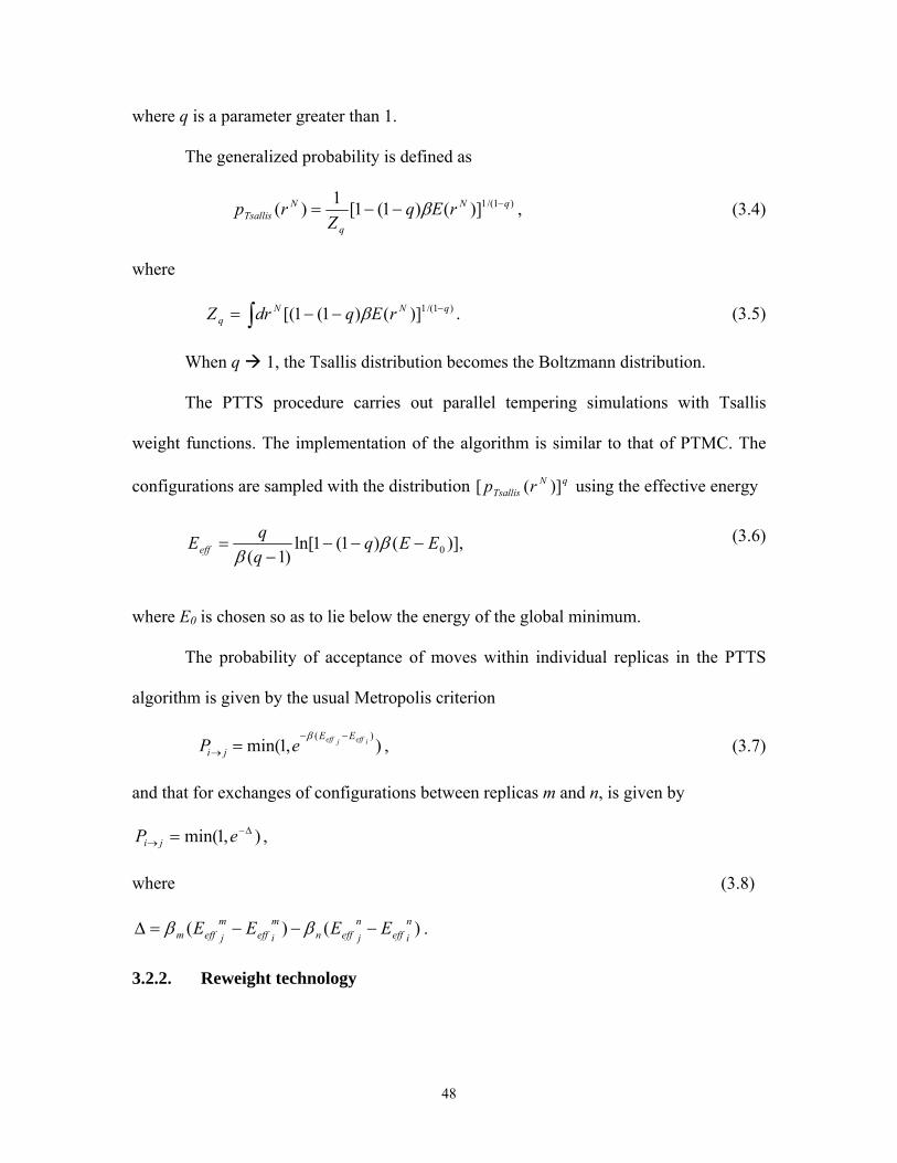
where q is a parameter greater than 1.
The generalized probability is defined as
)1/(1)]()1(1[1)( qN
q
NTsallis rEq
Zrp −−−= β , (3.4)
where
)1/(1)]()1(1[( qNNq rEqdrZ −∫ −−= β . (3.5)
When q 1, the Tsallis distribution becomes the Boltzmann distribution.
The PTTS procedure carries out parallel tempering simulations with Tsallis
weight functions. The implementation of the algorithm is similar to that of PTMC. The
configurations are sampled with the distribution using the effective energy qNTsallis rp )]([
(3.6) )],
((ln[ Eqq−−−= β)11
)1( 0Eq
Eeff −β
where E0 is chosen so as to lie below the energy of the global minimum.
The probability of acceptance of moves within individual replicas in the PTTS
algorithm is given by the usual Metropolis criterion
),1min()(
ieffjeff EEji eP
−−
→ =β
, (3.7)
and that for exchanges of configurations between replicas m and n, is given by
),1min( ∆−→ = eP ji ,
where (3.8)
)()( nieff
njeffn
mieff
mjeffm EEEE −−−=∆ ββ .
3.2.2. Reweight technology
48
Since the PTTS and TS simulations are carried out in a generalized ensemble, it is
essential to transform back to the canonical ensemble in order to obtain physically
meaningful values for the potential energy, heat capacity, and other properties of interest.
This is accomplished by histogram reweighting. In the histogram method, the frequency
of observing a energy range between bin is recorded which denoted H(E). E is the media
value f the energy range in the bin. The probability of observing a particular value E is
given by
EeEWZ
EP β−= )(1)( , (3.9)
where β=1/(kT), Z is the partition function, and W(E) is the number of states with energy
E.
If we generate Nc configurations, the expectation value of the number of
occurrences of E is given by
Ec eEWZNEH β−−= )()( 1 (3.10)
so
EZeEHEW β)()( = . (3.11)
Still consider the energy, the sampling over generalized Tsallis statics ensemble can be
reweight as:
∑∑
−−
−−
==
E
EEE
EE
eff
eff
eEH
eEEHEU )(
)(
)(
)(
β
β
, (3.12)
where Eeff is the effective energy is the Tsallis statistics.
The histogram procedure is very simple to implement, however the sum over all
energy levels can result in overflows. This problem can be solved by the strategy of Ref
49
5, in which the terms in equation 3.12 are calculated using logarithms. The basic idea is:
if l1 and l2 are the logarithms of two numbers x1 and x2, and that l1 ≥ l2, then the logarithm
of the sum x1 + x2 is
).1log())1(log()log()log( 1212121121
lllllll eleeeexx −− ++=+=+=+ (3.13)
3.3. Computational details
3.3.1. 1D model potential
We wish to compare the rates of convergence of parallel tempering Monte Carlo
(PTMC), parallel tempering Tsallis statistics (PTTS), Metropolis Monte Carlo (MMC)
and Tsallis statistics (TS). To accomplish this, we employ a 1D-model potential as a test.
Since the exact distribution can be calculated analytically for the model potential, the
ergodicity can be readily monitored throughout the simulation. The potential energy
function used is
∑=
−−−−+− +−−−=4
1
)3(3)2(3)8(100 )10/2sin(100.505.470.50)(222
nn
xxx xnCeeexV π ,
(3.14)
where x belongs to (-10, 10) and C1, C2, C3, C4 are chosen to be -0.466516, -0.834376,
-0.714529, and -0.0245586, respectively. A plot of the potential energy function is shown
in Figure 3.3, from which it is seen that it has two low-lying minima of almost the same
energy, one with a narrow funnel (global minimum) and one with a broad funnel.
The exact distribution is calculated explicitly from the formula:
∫ −
−
=)(
)(
)(xV
xV
exact dxeex
β
β
ρ . (3.15)
50
The numerical distribution corresponding to a simulation of length steps is
denoted by ).;( stepsxnumρ The ergodicity during the simulations is calculated using
∑∑ −
=
xexact
xexactnum
x
xstepsxsteps 2
2
2
)]([
)]();([)(
ρ
ρρχ . (3.16)
The simulations were carried out at temperatures of 24.0, 6.0, 1.5, 0.375, and
0.09375. In the PTMC and PTTS simulations exchanges between adjacent temperatures
were attempted every 500 moves. The highest temperature used, 24.0, is high enough to
avoid trapping even in the Metropolis MC simulations (as seen from Fig. 3.3). All
simulations were carried out for 108 moves at each temperature. The maxima step sizes of
the various simulations (MMC, TS, PTMC and PTTS) were adjusted to maintain a 50%
acceptance ratio during the simulations. The q values in the Tsallis statistic and parallel
tempering Tsallis statistics have been set to 1.1.
3.3.2. PTMC simulations of Ar38
The PTMC simulations of Ar38 carried out in the present study used the same 32
temperatures employed by Neirotti et al. Every 38th move an exchange of configurations
from replicas at adjacent temperatures (Ti and Ti+1) was attempted, with Ti also being
selected at random. This gave an attempted exchange rate of once every 38 x 31 moves,
approximately three times less frequent than that used in the study of Neirotti et al. The
remaining moves involved attempted displacements of individual atoms, selected at
random and with acceptance/rejection being based on the Metropolis procedure. In
carrying out PTMC simulations on cluster systems it is essential to exclude evaporative
events. This was accomplished in the present study by using a constraint sphere with a
radius of 8.5 Å. The maximum step sizes for the production runs were determined from
51
preliminary PTMC simulations in which the maximum step sizes were adjusted so that
about 50% of the moves were accepted in each replica.
To monitor convergence, the simulations were carried out for different length
equilibration periods, followed by production runs comprised of 109 move blocks. The
equilibration periods ranged from 0.4x10⁹ to 6.4x10⁹ moves. The heat capacity for each
simulation was calculated using
)(1 222 EE
kTCv −= . (3.17)
For each replica, every millionth configuration was saved for subsequent analysis.
3.3.3. PTTS simulations of Ar38
In our application of the PTTS algorithm we used the same temperature grid as
employed for the PTMC simulations. Evaporative events were again excluded by using a
8.5 Å constraint sphere. After completion of the simulation, the energies were reweighted
by using the histogram method99 to transform back to the canonical ensemble.
Hansmann et al.100 recommended choosing q = 1+1/N, where N is the number of
degrees of freedom, in the system of interest. In the case of Ar38 this would give q =
1.009. However, we were unable to achieve well converged results for our PTTS
simulations of Ar38 with a q value this large, and we adopted instead q = 1.001.
3.4. Results
3.4.1. 1D model potential
Figure 3.4 and 3.5 plot the ergodicity curves for the simulations carried out on the
1D model potential at different temperatures. The simulations were started from a
52
random position between x = 0 and x = 10, which are around the broad energy funnel.
The distributions during the simulation are calculated using the histogram method. A
total of 10,000 bins are used along the x axis, giving a bin size of 0.002. For T = 24 all
simulation methods rapidly achieve equilibrium. At T = 0.094, neither Metropolis Monte
Carlo nor Tsallis statistics sampling is able to achieve equilibrium even after 108 steps. In
particular, in this case the system remains localized in the broad funnel, and is unable to
sample the deeper, narrow funnel. In contrast, both PTMC and PTTS sample the
Boltzmann distribution with a relative error of less than 1% even for s as short as 5x10⁵
moves. For simulations longer than about 1x10⁷ moves, PTTS performs significantly
better than PTMC.
3.4.2. PTMC simulations of Ar38
Figures 3.6 and 3.7 report the heat capacity curves obtained from the PTMC
simulations initiated from the Oh and C5v minima, respectively. The various curves were
obtained from simulations with production periods of 1x10⁹ moves, and with
equilibration periods ranging from 0.4x10⁹ to 6.4x10⁹ moves. The curves from the
simulations starting from the global minimum (Fig. 3.1) are in fairly good agreement
with one another, with the greatest sensitivity to the length of the equilibration period
being for temperatures near 12 K, i.e., in the vicinity of the Oh icosahedral
transformation. The agreement in this case is even better if we consider only the
simulations with equilibration periods of 3.4x10⁹ or more moves. The remaining small
spread in the heat capacity curves near T = 12 K reflects the need for use of longer
production runs.
53
From a comparison of Fig. 3.6 and 3.7 it is seen that the agreement between the
heat capacity curves from the various simulations started from the C5v minimum is much
poorer than that found between the heat capacity curves from the various simulations
started from the Oh minimum. In particular, when starting from the C5v minimum, the
simulations employing equilibration periods of 0.4x10⁹, 1.4x10⁹, and 2.4x10⁹ moves
display a spurious peak at temperatures below that anticipated for the Oh icosahedral
transformation. This peak is especially pronounced in the simulation with an
equilibration period of only 0.4x10⁹ moves, where it appears near 3 K. The spurious peak
moves up in temperature and decreases in height as the equilibration period is increased,
approaching the physically meaningful shoulder near T =12 K for equilibration periods of
3.4x10⁹ or more moves. However, even when using these longer equilibration periods,
the heat capacity curves from the various simulations show more scatter, especially in the
region of the Oh icosahedral transformation, when starting from the C5v than from the
Oh minimum. This indicates that the need for a longer production period is more acute
when starting the simulation from the C5v minimum.
Figure 3.8 displays heat capacity curves obtained from PTMC simulations starting
from the global minimum and from the C5v minimum, with equilibration periods of
3.4x10⁹ moves and averaging over four consecutive blocks of 1x10⁹ production moves.
The two heat capacity curves are in close agreement with one another as well as with that
published previously by Neirotti et al. even in the region of the shoulder due to the Oh
icosahedral transformation. However, the agreement is deceptive as is revealed by
comparing with the results obtained from still longer simulations with averages
calculated using the configurations sampled in the moves between 7.4x10⁹ and 11.4x10⁹
54
and between 11.4x10⁹ and 17.4x10⁹. For the case that the simulations were started from
the global minimum, the resulting heat capacity curves are nearly identical to that
obtained by averaging over the configurations sampled over the moves 3.4x10⁹ to
7.4x10⁹ and which is shown in Fig. 3.8. On the other hand, in the case that the
simulations were started from the second lowest energy minimum, the heat capacity
curve obtained by averaging over configurations sampled in the 7.4x10⁹ to 11.4x10⁹
range of moves is much more pronounced than that reported in Fig. 3.8, whereas that
obtained by averaging over moves in the 11.4x10⁹ – 17.4x10⁹ range is similar to that
reported in Fig. 3.8. These results show that very long production runs are required to
achieve convergence of PTMC simulations in the vicinity of the Oh icosahedral
transformation when starting from the C5v minimum.
Additional insight into the origin of the difficulty in converging the PTMC
simulations of LJ38 when starting from the C5v minimum can be gained by determining
the inherent structures associated with the configurations present at the end of each
equilibration period. The inherent structures were obtained by optimized the structures
with the eigenmode-following algorithm as implemented in the Orient program.101
Figure 3.9a reports for the simulations starting from the global minimum the energies of
the resulting inherent structure at the end of various equilibration periods. The resulting
inherent structure distributions are similar for various length equilibration periods, with
the first ten replicas (i.e., those for the ten lowest temperatures) giving the global
minimum and at most three of the 17 lowest temperature replicas giving an inherent
structure other than the global minimum. Similar results are found for the inherent
structures populated at the end of the production runs for the simulations starting from the
55
C5v local minimum for the cases of equilibration periods of 3.4x10⁹ or more moves. (Fig.
3.9b) However, in the simulations with equilibration periods of 2.4x10⁹ or fewer moves,
fewer low-temperature replicas have inherent structure associated with the global
minimum at the end of the equilibration runs. In fact, with the equilibration period of
only 0.4x10⁹ moves, only the lowest temperature replica is associated with the global
minimum inherent structure at the end of the equilibration. As the production runs
increase from 4x10⁸ to 3.4x10⁹ moves, the number of low-temperature replicas associated
with the global minimum at the end of the run increases. The spurious low-temperature
peak in the heat capacity curve in the simulations starting from the second lowest energy
minimum structure and with equilibration periods of less than 3.4x10⁹ moves, is a
consequence of the global minimum structure not being adequately sampled in the
equilibration runs in the low-temperatures replicas. In these cases, during the course of
the production runs, there is a shift in the population in the low temperature replicas from
minima in the icosahedral funnel to the Oh funnel. This shift in population is responsible
for the spurious low-temperature peak in Cv. While this problem could be overcome by
use of very long production cycles, this is less computationally efficient than using
equilibration runs of adequate length.
We next examine the distributions of inherent structures obtained from the
production runs associated with PTMC simulations starting from both the global
minimum structure as well as from the C5v minimum. Fig. 3.10 shows the distributions
obtained for the simulations started from the C5v local minima, using production runs of
1x10⁹ moves, and employing various length equilibration periods. For each simulation,
every millionth configuration was saved and optimized to its inherent structure. It is clear
56

from the results reported in this figure that the simulations using equilibration periods of
only 1.4x10⁹ and 2.4x10⁹ moves are far from converged.
Fig. 3.11 reports the distributions of inherent structures from simulation starting
from the Oh and C5v minima, and carried out for equilibration periods of 3.4x10⁹ moves
and production periods of 4x10⁹ moves. The inherent structure distributions from these
two simulations are nearly identical although, as pointed out above, simulations starting
from the second lowest energy minimum are not actually converged. The population of
low-energy structures associated with the icosahedral funnel grows rapidly as the
temperature increases from about 10 K, and reaches a maximum around 18 K.
Interestingly, both the third and fifth lowest energy isomers of Ar38 acquire considerably
more population than does the second-lowest energy (C5v) isomer. At T = 18.5 K, 65% of
the total population is associated with the four-lowest energy inherent structures
associated with the icosahedral funnel.
3.4.3. PTTS simulations of Ar38
Figure 3.12 shows the heat capacity curves obtained from the PTTS simulations
of Ar38 initiated from the second lowest energy minimum. The equilibration periods
ranged from 0.4 to 3.2x10⁹ moves and the production cycles were either 1.0x10⁹ or
0.6x10⁹ moves. PTTS simulations with an equilibration period as short as 2.0x10⁹ moves
and a production period as short as 0.6x10⁹ moves, give a nearly converged Cv vs. T
curve, with the exception being that the shoulder near 12 K is slightly more pronounced
than found from the PTMC simulations starting from the global minimum. Upon adoption
of an equilibration period of 3.2x10⁹ moves, while remaining a production period of only
0.6x10⁹ moves, the low-temperature shoulder is attenuated, bringing it more in line with
57
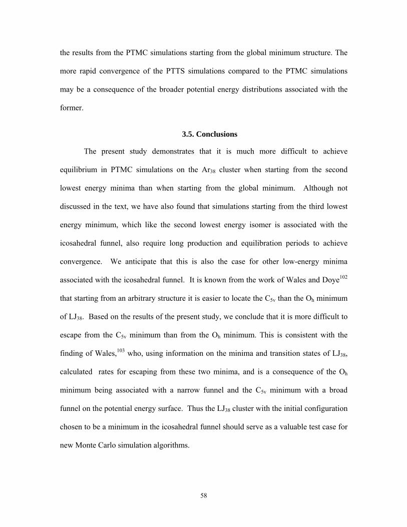
the results from the PTMC simulations starting from the global minimum structure. The
more rapid convergence of the PTTS simulations compared to the PTMC simulations
may be a consequence of the broader potential energy distributions associated with the
former.
3.5. Conclusions
The present study demonstrates that it is much more difficult to achieve
equilibrium in PTMC simulations on the Ar38 cluster when starting from the second
lowest energy minima than when starting from the global minimum. Although not
discussed in the text, we have also found that simulations starting from the third lowest
energy minimum, which like the second lowest energy isomer is associated with the
icosahedral funnel, also require long production and equilibration periods to achieve
convergence. We anticipate that this is also the case for other low-energy minima
associated with the icosahedral funnel. It is known from the work of Wales and Doye102
that starting from an arbitrary structure it is easier to locate the C5v than the Oh minimum
of LJ38. Based on the results of the present study, we conclude that it is more difficult to
escape from the C5v minimum than from the Oh minimum. This is consistent with the
finding of Wales,103 who, using information on the minima and transition states of LJ38,
calculated rates for escaping from these two minima, and is a consequence of the Oh
minimum being associated with a narrow funnel and the C5v minimum with a broad
funnel on the potential energy surface. Thus the LJ38 cluster with the initial configuration
chosen to be a minimum in the icosahedral funnel should serve as a valuable test case for
new Monte Carlo simulation algorithms.
58

A new algorithm combining parallel tempering Monte Carlo and Tsallis statistics
is introduced and tested on a 1 – dimensional model potential and on LJ38. The model
potential results demonstrate significantly better convergence of the PTTS algorithm than
for the PTMC algorithm. The PTTS algorithm also displays improved convergence in the
case of LJ38. Further work is needed to determine whether this hybrid algorithm will in
fact require fewer temperatures than does the PTMC algorithm.
59
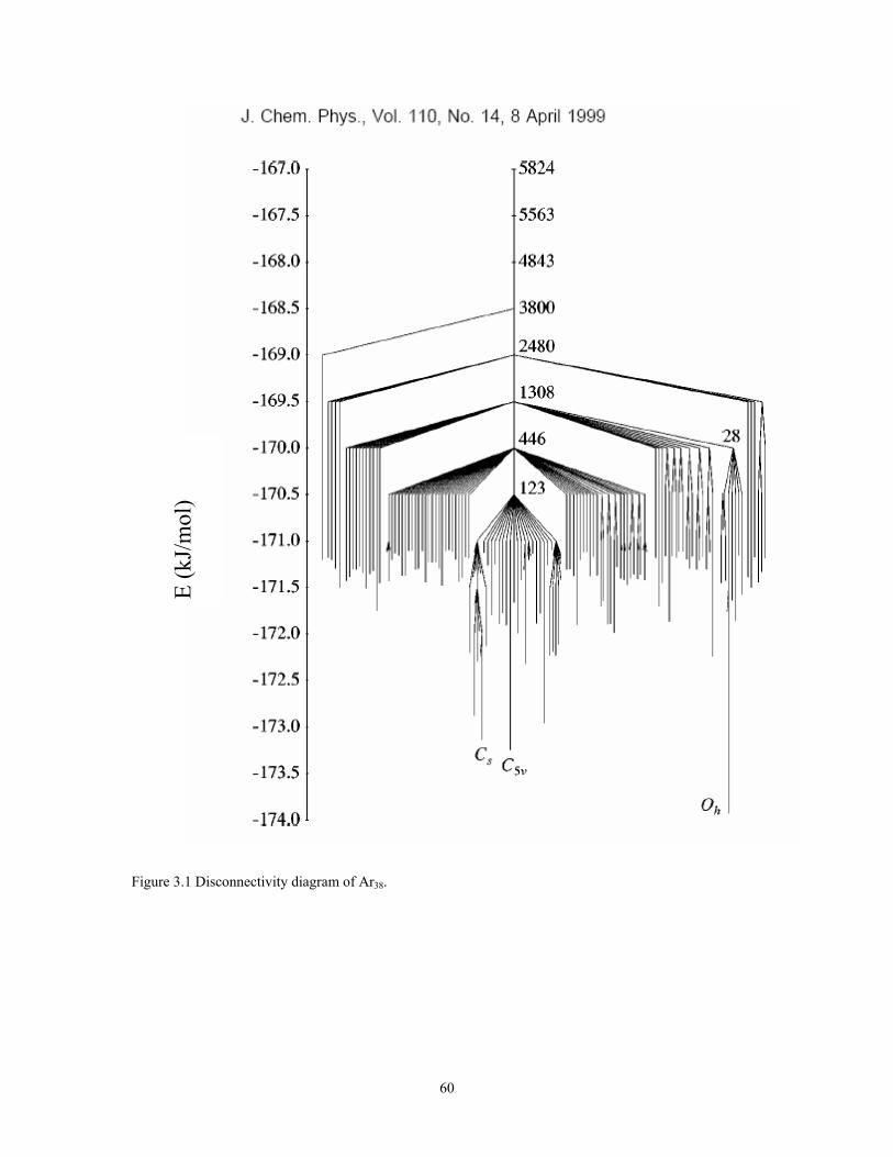
E (k
J/m
ol)
Figure 3.1 Disconnectivity diagram of Ar38.
60
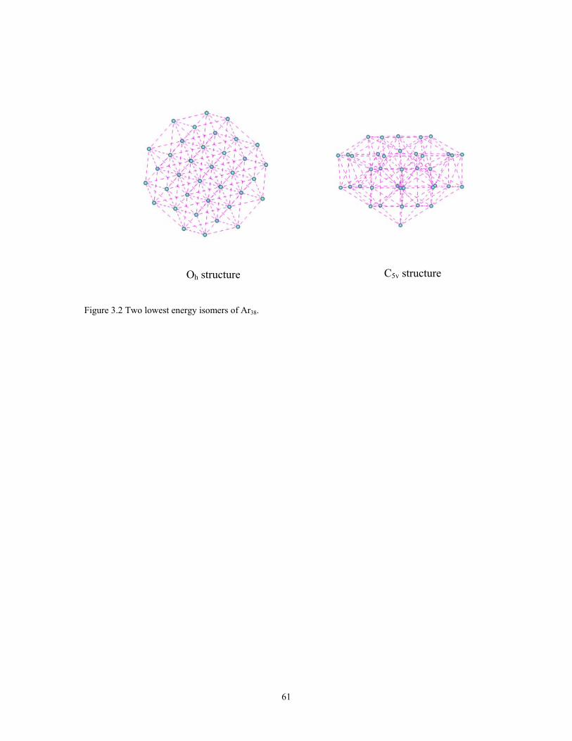
e e
Figure 3.2 Two lowest ene
Oh structur
rgy isomers of Ar38.
61
C5v structur
10 5 0 5 1060
40
20
0
20
V(x) ρ(x)
--------- V(x) --------- ρ2(x) ---------- ρ1(x)*50
Figure 3.3 One-dimensional potential energy V(x) vs. position x and the analytical distributions ρ1 and ρ2 at T = 24 and 0.094, respectively.
62
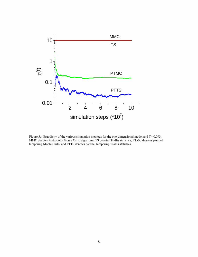
2 4 6 8 100.01
0.1
1
10
PTTS
PTMC
TS
MMC
simulation steps (*107)
χ(t)
Figure 3.4 Ergodicity of the various simulation methods for the one-dimensional model and T= 0.093. MMC denotes Metropolis Monte Carlo algorithm, TS denotes Tsallis statistics, PTMC denotes parallel tempering Monte Carlo, and PTTS denotes parallel tempering Tsallis statistics.
63
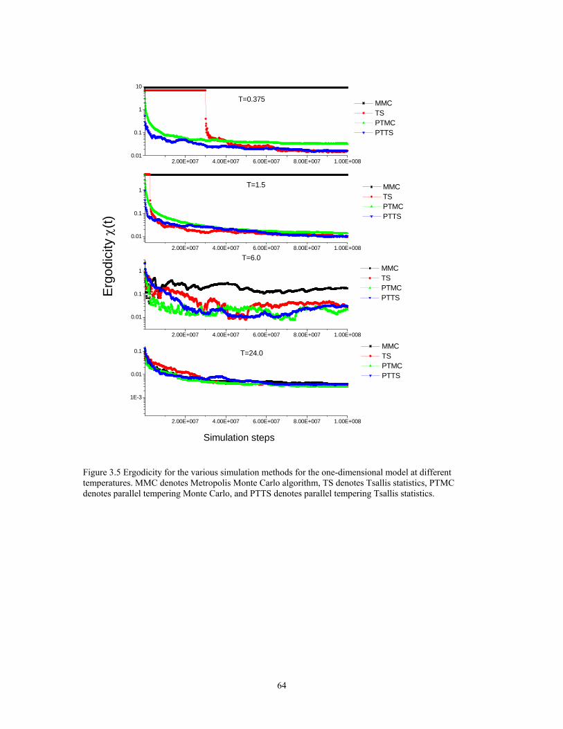
2.00E+007 4.00E+007 6.00E+007 8.00E+007 1.00E+008
1E-3
0.01
0.1
Ergo
dici
ty χ
(t)
T=24.0 MMC TS PTMC PTTS
Simulation steps
2.00E+007 4.00E+007 6.00E+007 8.00E+007 1.00E+008
0.01
0.1
1
T=6.0 MMC TS PTMC PTTS
2.00E+007 4.00E+007 6.00E+007 8.00E+007 1.00E+008
0.01
0.1
1T=1.5 MMC
TS PTMC PTTS
2.00E+007 4.00E+007 6.00E+007 8.00E+007 1.00E+0080.01
0.1
1
10
T=0.375 MMC TS PTMC PTTS
Figure 3.5 Ergodicity for the various simulation methods for the one-dimensional model at different temperatures. MMC denotes Metropolis Monte Carlo algorithm, TS denotes Tsallis statistics, PTMC denotes parallel tempering Monte Carlo, and PTTS denotes parallel tempering Tsallis statistics.
64
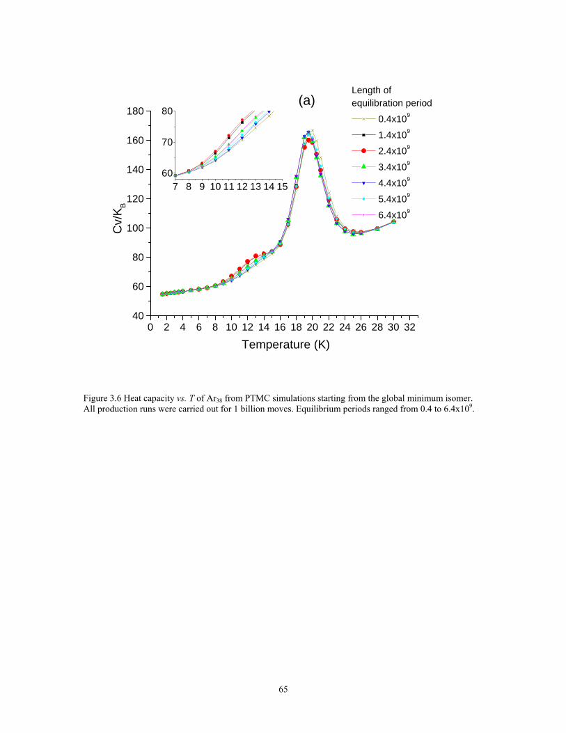
0 2 4 6 8 10 12 14 16 18 20 22 24 26 28 30 3240
60
80
100
120
140
160
180 C
v/K B
Temperature (K)
Length of equilibration period
0.4x10⁹
1.4x10⁹
2.4x10⁹
3.4x10⁹
4.4x10⁹
5.4x10⁹
6.4x10⁹
7 8 9 10 11 12 13 14 1560
70
80(a)
Figure 3.6 Heat capacity vs. T of Ar38 from PTMC simulations starting from the global minimum isomer. All production runs were carried out for 1 billion moves. Equilibrium periods ranged from 0.4 to 6.4x10⁹.
65

0 2 4 6 8 10 12 14 16 18 20 22 24 26 28 30 3240
60
80
100
120
140
160
180
Length ofequilibration period
0.4x10⁹
1.4x10⁹
2.4x10⁹
3.4x10⁹
4.4x10⁹
5.4x10⁹
6.4x10⁹
Temperature (K)
Cv
/KB
7 8 9 10 11 12 13 14 1560
70
80(b)
Figure 3.7 Heat capacity vs. T of Ar38 from PTMC simulations starting from second lowest energy minimum isomer. All production runs were carried out for 1 billion moves. Equilibrium periods ranged from 0.4 to 6.4x10⁹.
66
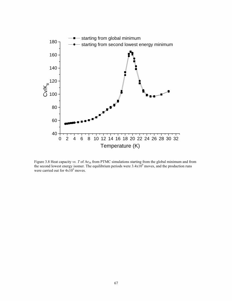
0 2 4 6 8 10 12 14 16 18 20 22 24 26 28 30 3240
60
80
100
120
140
160
180 C
v/K B
Temperature (K)
starting from global minimum starting from second lowest energy minimum
Figure 3.8 Heat capacity vs. T of Ar38 from PTMC simulations starting from the global minimum and from the second lowest energy isomer. The equilibrium periods were 3.4x10⁹ moves, and the production runs were carried out for 4x10⁹ moves.
67
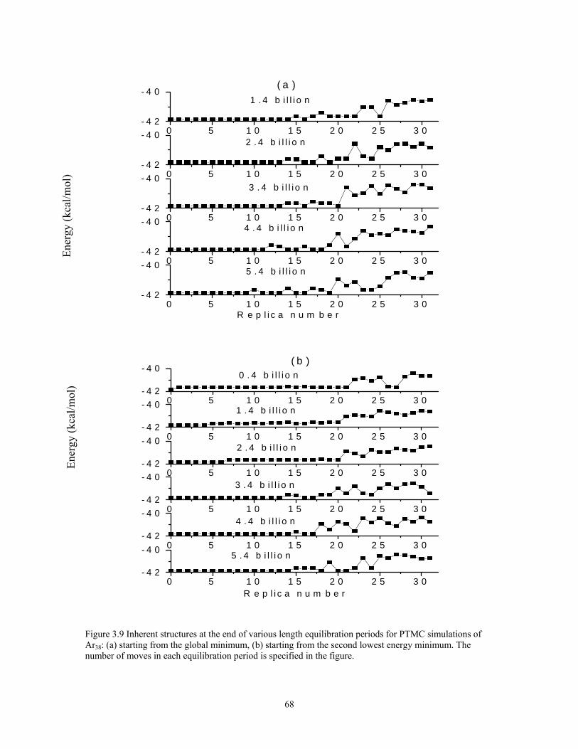
0 5 1 0 1 5 2 0 2 5 3 0- 4 2
- 4 05 . 4 b i l l i o n
0 5 1 0 1 5 2 0 2 5 3 0- 4 2
- 4 0
4 . 4 b i l l i o n0 5 1 0 1 5 2 0 2 5 3 0
- 4 2
- 4 03 . 4 b i l l i o n
0 5 1 0 1 5 2 0 2 5 3 0- 4 2
- 4 0
2 . 4 b i l l i o n0 5 1 0 1 5 2 0 2 5 3 0
- 4 2
- 4 0
R e p l i c a n u m b e r
( a )1 . 4 b i l l i o n
Ener
gy (k
cal/m
ol)
0 5 1 0 1 5 2 0 2 5 3 0- 4 2
- 4 0 5 . 4 b i l l i o n0 5 1 0 1 5 2 0 2 5 3 0
- 4 2
- 4 04 . 4 b i l l i o n
0 5 1 0 1 5 2 0 2 5 3 0- 4 2
- 4 03 . 4 b i l l i o n
0 5 1 0 1 5 2 0 2 5 3 0- 4 2
- 4 0
2 . 4 b i l l i o n0 5 1 0 1 5 2 0 2 5 3 0
- 4 2
- 4 0 1 . 4 b i l l i o n0 5 1 0 1 5 2 0 2 5 3 0
- 4 2
- 4 0
R e p l i c a n u m b e r
( b )0 . 4 b i l l i o n
Ener
gy (k
cal/m
ol)
Figure 3.9 Inherent structures at the end of various length equilibration periods for PTMC simulations of Ar38: (a) starting from the global minimum, (b) starting from the second lowest energy minimum. The number of moves in each equilibration period is specified in the figure.
68

0 4 8 12 16 20 24 280.0
0.2
0.4
0.6
0.8
1.0 equilib. 1.4 billion moves
0 4 8 12 16 20 24 280.0
0.2
0.4
0.6
0.8
1.0 equilib. 2.4 billion moves
0 4 8 12 16 20 24 280.0
0.2
0.4
0.6
0.8
1.0
equilib. 3.4 billion moves
0 4 8 12 16 20 24 280.0
0.2
0.4
0.6
0.8
1.0 equilib. 4.4 billion moves
0 4 8 12 16 20 24 280.0
0.2
0.4
0.6
0.8
1.0 equilib. 5.4 billion moves
0 4 8 12 16 20 24 280.0
0.2
0.4
0.6
0.8
1.0
Pop
ulat
ion
Replica numberReplica number
equilib. 6.4 billion moves
Figure 3.10 Inherent structure distributions from PTMC simulations of Ar38 starting from the second lowest energy minimum. Simulations were carried out with a production period of 1×10⁹ moves and differ in the length of the equilibrium period. The inherent structures are labeled as follows: E = -41.821 (■), -41.659 (●), -41.630 (▲), -41.588 (▼), -41.569 (♦) and > -41.569 kcal/mol (+). The inherent structures with energies of -41.821 and -41.659 kcal/mol are the global minimum and the second lowest energy minimum, respectively.
69
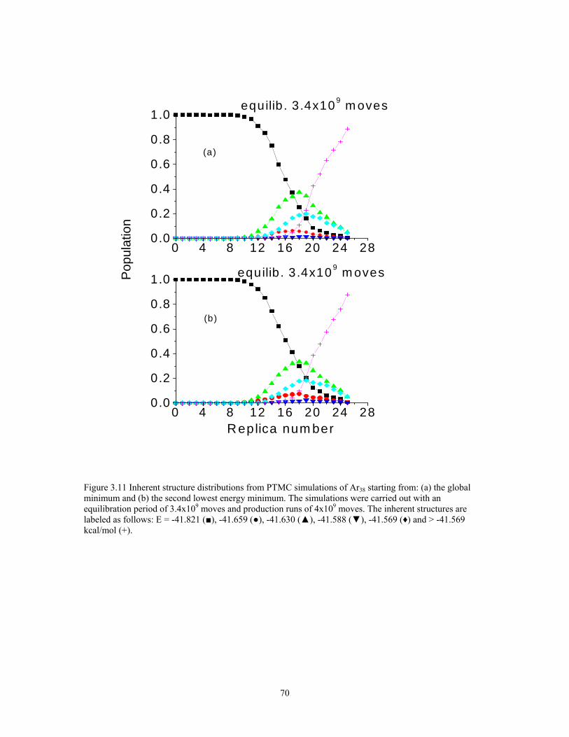
0 4 8 12 16 20 24 280.0
0.2
0.4
0.6
0.8
1.0
(b)
equilib . 3.4x10⁹ m oves
0 4 8 12 16 20 24 280.0
0.2
0.4
0.6
0.8
1.0P
opul
atio
n
Replica num ber
equilib . 3.4x10⁹ m oves
(a)
Figure 3.11 Inherent structure distributions from PTMC simulations of Ar38 starting from: (a) the global minimum and (b) the second lowest energy minimum. The simulations were carried out with an equilibration period of 3.4x10⁹ moves and production runs of 4x10⁹ moves. The inherent structures are labeled as follows: E = -41.821 (■), -41.659 (●), -41.630 (▲), -41.588 (▼), -41.569 (♦) and > -41.569 kcal/mol (+).
70

0 2 4 6 8 10 12 14 16 18 20 22 24 26 28 30 3240
60
80
100
120
140
160
180
equilib 4x10⁸
equilib 1.4x10⁹
equilib 2.0x10⁹
equilib 2.6x10⁹
equilib 3.2x10⁹
Cv/K
B
Temperature(K)
Figure 3.12 Heat capacity vs. T of Ar38 from PTTS simulations starting from the second lowest energy minimum. Equilibration periods ranged from 0.4x10⁸ to 2.6x10⁹ moves, and production periods were 1x10⁹ moves for the case of an equilibration period of 0.4x10⁸ moves and 0.6x10⁹ moves in the other four cases.
71
4. Chapter 4 The application of Wang-Laudau free random walk algorithm on Ar cluster
4.1. Introduction
Simulations of systems with rough potential energy surfaces pose considerable
challenges. Examples include high-density or low-temperature liquids, polymers, and
proteins, for which the simulation is prone to be trapped in potential energy minima for
large numbers of simulation steps. As mentioned in Chapter 1, numerous techniques have
been proposed to overcome the quasi-ergodicity problem associated with rough
landscapes and high energy barriers between energy minima. Techniques such as parallel
tempering and multicanonical Monte Carlo have proven to be valuable. Multicanonical
Monte Carlo simulations sample broad phase space by (ideally) using a uniform energy
distribution. The trapping into energy minima can be artificially eliminated by assigning
“weight” to different energy states. However the weight factors are not known so the
multicanonical computation often requires tedious iterative calculations to get a good
estimate of the weight factors.
As we have mentioned in Chapter 1, the Wang-Landau method directly and self-
consistently determines the density of states by performing a random walk in the energy
space. The WL algorithm has attracted a lot of attention, and it has been applied to
biological systems and to quantum Monte Carlo calculations. The application of WL
algorithm is very straightforward. The algorithm is also parallizable. Rathore et al.104
have combined the WL algorithm and the parallel tempering scheme in their studies of
the α-helix-coil and β-sheet-coil transitions of a designer peptide. Several new
approaches105,106 based on modifications of the WL algorithm have been published
recently.
72
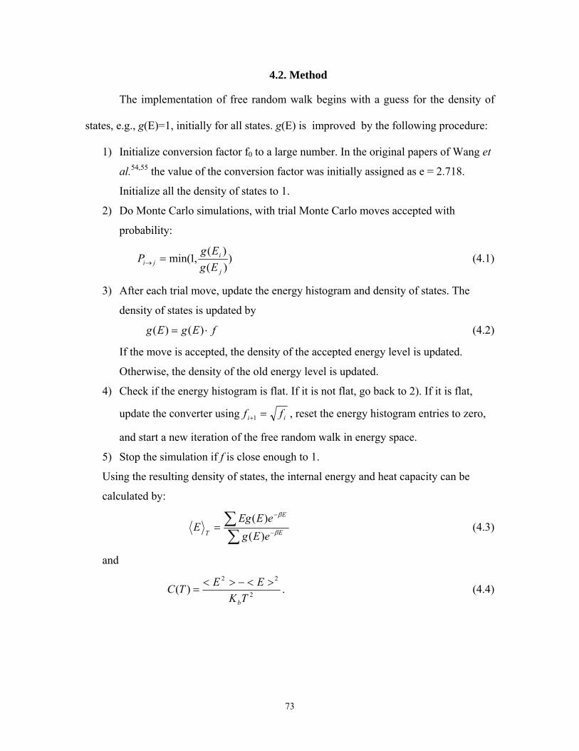
4.2. Method
The implementation of free random walk begins with a guess for the density of
states, e.g., g(E)=1, initially for all states. g(E) is improved by the following procedure:
1) Initialize conversion factor f0 to a large number. In the original papers of Wang et
al.54,55 the value of the conversion factor was initially assigned as e = 2.718.
Initialize all the density of states to 1.
2) Do Monte Carlo simulations, with trial Monte Carlo moves accepted with
probability:
))()(
,1min(j
iji Eg
EgP =→ (4.1)
3) After each trial move, update the energy histogram and density of states. The
density of states is updated by
fEgEg ⋅= )()( (4.2)
If the move is accepted, the density of the accepted energy level is updated.
Otherwise, the density of the old energy level is updated.
4) Check if the energy histogram is flat. If it is not flat, go back to 2). If it is flat,
update the converter using ii ff =+1 , reset the energy histogram entries to zero,
and start a new iteration of the free random walk in energy space.
5) Stop the simulation if f is close enough to 1.
Using the resulting density of states, the internal energy and heat capacity can be
calculated by:
∑∑
−
−
= E
E
T eEgeEEg
E β
β
)()(
(4.3)
and
2
22
)(TK
EETCb
><−><= . (4.4)
73
4.3. Simulation details
The WL free random walk algorithm was originally tested to investigate phase
transition of the Ising model54. After that, a number of groups have applied this method to
applications include protein,107 polymer films.108,109 Thus far there is no report of the
application of the WL algorithm to investigate the thermodynamic properties of clusters.
One of the most intriguing aspects of this approach is that density of states can be
used to obtain an estimate of the entropy. In this chapter, the WL free random walk
algorithm is applied to the Ar13 and to the much more complicated Ar38 cluster.
The thermodynamic properties of Ar13 have been explored with a wide range of
algorithms.30,33,91 The system is defined by Lennard Jones interactions. In our
simulations, a constraint sphere of 5 Å has been applied to the cluster. A single atom of
Ar is chosen at random and moved to a new position. The maximum step size is 0.5 Å.
The energy of the trial system is calculated and the probability of accepting the move is
based on equation 4.1. The system is allowed to move in the energy range of -10.7
kcal/mol to 0 kcal/mol. A total 50 bins were used to divide up the energy range.
The free random walk algorithm was also applied to Ar38. In this case the
constraint sphere was chosen to be 8.5 Å. The energy range in the simulation is from -
41.3 kcal/mol to -30 kcal/mol. The energy range was binned with a bin-size of 0.2
kcal/mol. For the Ar38 cluster it is difficult to get a flat energy distribution, at least when
using single atom moves. Since the system is allowed to move freely in the energy space,
the acceptance ratio is proportional to the density of states. If the energy of a newly
generated configuration fills within an energy bin which has not been visited before, the
move will definitely be accepted. However, randomly generating configurations at the
low energies is much more difficult than at high energies, particularly for the systems
74
with sharp funnels in their potential energy surface. A second approach has been tested
for updating configurations. A pivot (reflection point within the constraint sphere) was
randomly chosen, then the atoms within the distance of 3.5 Å of the pivot are subject to a
reflection with respect to the pivot. The group and reflection method for updating the
configurations has been applied in the geometric cluster algorithms developed by Luijten
et al.110 Such multiple-moves are very useful in some cases since they keep the basic
interactions within the group (e.g., in the water cluster, the reflection would retain
hydrogen bonds within the group).
Even with the geometry group scheme to update the configurations, it is still not
possible to get a flat energy distribution in the region of the global and second lowest
energy minima. In the simulation of Ar38, The energy range to do free random walk is -
41.3 kcal/mol to -30 kcal/mol.
4.4. Results and discussion
Figure 4.1 compares the heat capacity curve of Ar13 calculated using WL
algorithm and with jump walk Monte Carlo method. It has been established that jump
walk algorithm is suitable for Ar13 system33. 16 temperatures were used in the jump-walk
Monte Carlo simulations. Overall there is a fair agreement between the heat capacity
curves calculated using the two approaches. WL simulations are much faster to converge
and do not depend on the spacing of the temperature grid. Basically you can calculate any
thermodynamic properties at any temperature in the free random walk algorithm.
However for Ar38 the heat capacity curve calculated using the free random walk
procedure is only in fair agreement with the PTTS curve depicted earlier. Figure 4.2
compares the heat capacity curve of Ar38 calculated using WL algorithm and PTTS
75
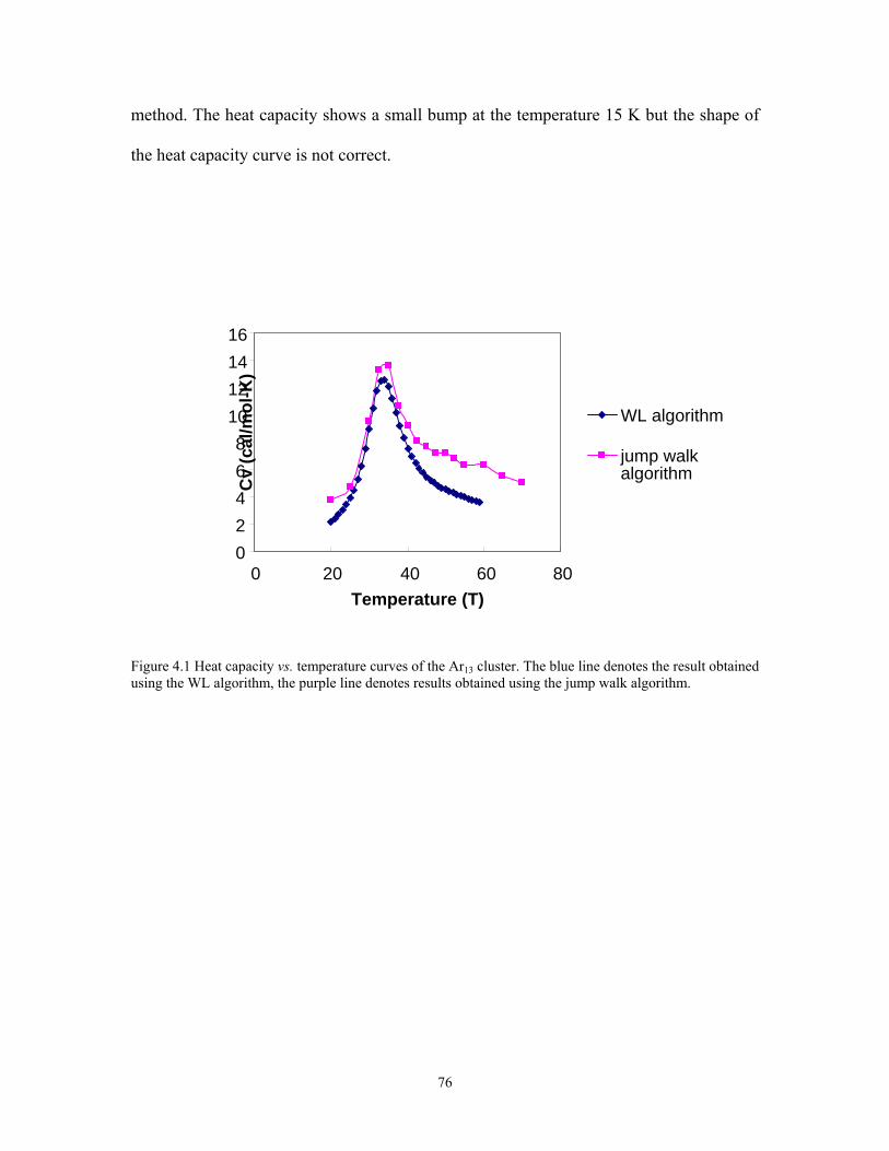
method. The heat capacity shows a small bump at the temperature 15 K but the shape of
the heat capacity curve is not correct.
16 14
Figure 4.1 Heat capacity vs. temperature curves of the Ar13 cluster. The blue line denotes the result obtained using the WL algorithm, the purple line denotes results obtained using the jump walk algorithm.
0 2 4 6
Cv
(
8 cal/
10 mo
12 l-K)
WL algorithm
jump walk algorithm
0 20 40 60 80Temperature (T)
76

0
1
2
3
4
5
6
7
8
9
0 10 20 30 40 50
Temperature(K)
Cv(
cal/m
ol-K
)
WL algorithmPTTS
Figure 4.2 Heat capacity vs. temperature curve of Ar38 obtained using the WL algorithm and PTTS algorithm.
77
BIBLIOGRAPHY
(1) Metropolis, N. “Monte Carlo: in the beginning and some great expectations,” in Monte Carlo Calculations and Applications in Neutronics, Photonics, and Statistical Physics, edited by Alcouffe, R., Dautray R., Forster A. Ledanois G. and Mercier, B. Springer Verlag: Berlin, 1985.
(2) Metropolis, N. Los Alamos Science 1987.
(3) Frenkel, D. and Smit, B. Understanding Molecular Simulation; Academic Press: San Diego, 1996.
(4) Kalos, M. H. and Whitlock, P. A. Monte Carlo methods; Wiley-interscience: New York, 1986.
(5) Newman, M. E. J. and Barkema, G. T. Monte Carlo Methods in Statistical Physics; Oxford Univ. Press: New York, 2001.
(6) Metropolis, N., Rosenbluth, A. W., Rosenbluth, M. N., Teller, A. H. and Teller, E. J. Chem.Phys. 1953, 21, 1087.
(7) Berne, B. J. and Straub, J. E. Curr. Opin. Struc. Bio. 1997, 7, 181.
(8) Mitsutake, A., Sugita, Y. and Okamoto, Y. Biopolymers (peptide science) 2001, 60.
(9) Berg, B. Phys. Commun. 2002, 104.
(10) Torrie, G. M. and Valleau, J. P. J. Comput. Phys. 1977, 23, 187.
(11) Lee, J. Phys. Rev. Lett. 1993, 71, 211.
(12) Beichl, I. and Sulivan, F. Computing in Science & Engineering 1999, 1, 71.
(13) Bigot, B. and Jorgensen, W. L. J. Chem. Phys. 1981, 75, 1944.
(14) Ding, K. and Valleau, J. P. J. Chem. Phys. 1993, 98, 3306.
(15) Berg, B. A. Int'l J. Mod. Phys. C 1993, 4, 249.
(16) Berg, B. A. Comput. Phys. Commun. 2003, 153, 397.
78
(17) Yasar, F., Arkin, H., Celik, T., Berg, B. A. and Meirovitch, H. J. Comput. Chem. 2002, 23, 1127.
(18) Arkin, H., Yasar, F., Celik, T., Berg, B. A. and Meirovitch, H. Comput. Phys. Commun. 2002, 147, 600.
(19) Berg, B. A. Nuclear Phys. B, Proceedings Supplements 1998, 63, 982.
(20) Berg, B. A., Hansmann, U. E. and Celik, T. Phys. Rev. B 1994, 50, 16444.
(21) Berg, B. A., Celik, T. and Hansmann, U. Europhys. Lett. 1993, 22, 63.
(22) Holzlohner, R. and Menyuk Curtis, R. Opt. Lett. 2003, 28, 1894.
(23) Gil Kim, J., Fukunishi, Y., Kidera, A. and Nakamura, H. Phys. Rev. E 2003, 68, 021110.
(24) Shirai, H., Nakajima, N., Higo, J., Kidera, A. and Nakamura, H. J. Mol. Biol. 1998, 278, 481.
(25) Straub, J. E. and Andricioaei, I. Brazilian. J. Phys. 1999, 29, 179.
(26) Andricioaei, I. and Straub, J. E. J. Chem. Phys. 1997, 107, 9117.
(27) Andricioaei, I. and Straub, J. E. Phys. Rev. E 1996, 53, R3055.
(28) Tsallis, C. and Stariolo, D. A. Physica A 1996, 233, 395.
(29) Frantz, D. D. J Chem. Phys. 2001, 115, 6136.
(30) Frantz, D. D., Freeman, D. L. and Doll, J. D. J. Chem. Phys. 1992, 97, 5713.
(31) Frantz, D. D. J. Chem. Phys. 1996, 105, 10030.
(32) Frantz, D. D. J. Chem. Phys. 1997, 107, 1992.
(33) Tsai, C. J. and Jordan, K. D. J. Chem. Phys. 1993, 99, 6957.
(34) Geyer, C. J. and Thompson, E. A. J. Am. Stat. Assoc. 1995, 90, 909.
(35) Tesi, M. C., van Fensburg, E. J. J., Orlandini, E. and Whittington, S. G. J. Stat. Phys. 1996, 82, 155.
(36) Hukushima, K. and Nemoto, K. J. Phys. Soc. Jpn. 1996, 65, 1604.
(37) Hukushima, K., Takayama, H. and Nemoto, K. Int. J. Mod. Phys. C 1996, 7, 337.
79
(38) Habeck, M., Nilges, M. and Rieping, W. Phys. Rev. Lett. 2005, 94.
(39) Yang, X. and Saven, J. G. Chem. Phys. Lett. 2005, 401, 205.
(40) Chen, J. H., Im, W. and Brooks, C. L. J. Am. Chem. Soc. 2004, 126, 16038.
(41) Cecchini, M., Rao, F., Seeber, M. and Caflisch, A. J. Chem. Phys. 2004, 121, 10748.
(42) Ahunbay, M. G., Kranias, S., Lachet, V. and Ungerer, P. Fluid Phase Equilib. 2004, 224, 73.
(43) Sabo, D., Predescu, C., Doll, J. D. and Freeman, D. L. J. Chem. Phys. 2004, 121, 856.
(44) Hung, F. R., Dudziak, G., Sliwinska-Bartkowiak, M. and Gubbins, K. E. Mole. Phys. 2004, 102, 441.
(45) Vreede, J., Bolhuis, P. G., Smit, B. and Hellingwerf, K. J. Biophys. J. 2004, 86, 84A.
(46) Fenwick, M. K. and Escobedo, F. A. J. Chem. Phys. 2003, 119, 11998.
(47) Im, W., Feig, M. and Brooks, C. L. Biophys. J. 2003, 85, 2900.
(48) Suenaga, A. J. Mol. Structure-Theochem 2003, 634, 235.
(49) Pitera, J. W. and Swope, W. Proc. Natl. Acad. Sci. U. S. A. 2003, 100, 7587.
(50) Sikorski, A. and Romiszowski, P. Biopolymers 2003, 69, 391.
(51) Pokarowski, P., Kolinski, A. and Skolnick, J. Biophys. J. 2003, 84, 1518.
(52) Bratko, D. and Blanch, H. W. J. Chem. Phys. 2003, 118, 5185.
(53) Zhou, R. H., Berne, B. J. and Germain, R. Proc. Natl. Acad. Sci. U. S. A. 2001, 98, 14931.
(54) Wang, F. G. and Landau, D. P. Phys. Rev. E 2001, 64.
(55) Wang, F. G. and Landau, D. P. Phys. Rev. Lett. 2001, 86, 2050.
(56) Hetenyi, B., Bernacki, K. and Berne, B. J. J. Chem. Phys. 2002, 117, 8203.
(57) Stolovitzky, G. and Berne, B. J. Proc. Natl. Acad. Sci. U. S. A. 2000, 97, 11164.
80
(58) Brown, S. and Head-Gordon, T. J. Comput. Chem. 2003, 24, 68.
(59) Swendsen, R. H., Diggs, B., Wang, J. S., Li, S. T., Genovese, C. and Kadane, J. B. Inter.l J Modern Phys.s C 1999, 10, 1563.
(60) Wang, J. S. Comput. Phys. Commun. 1999, 122, 22.
(61) Wang, J. S., Tay, T. K. and Swendsen, R. H. Phys. Rev. Lett. 1999, 82, 476.
(62) Stone, A. J. the theory of Intermolecular Forces; Calrendon Press: Oxford, 1996.
(63) Kobashi, K. and Kihara, T. J. Chem. Phys. 1980, 3216.
(64) Etters, R. D. and Kuchta, B. J. Chem. Phys. 1989, 90, 4537.
(65) Kuchta, B. and Etters, R. D. Phys. Rev. B 1988, 38, 6265.
(66) Etters, R. D., Flurchick, K., Pan, R. P. and Chandrasekharan, V. J. Chem. Phys. 1981, 75, 929.
(67) Torchet, G., de Feraudy, M. F., Boutin, A. and Fuchs, A. H. J. Chem. Phys. 1996, 105, 3671.
(68) Maillet, J.-B., Boutin, A., Buttefey, S., Calvo, F. and Fuchs, A. H. J. Chem. Phys. 1998, 109, 329.
(69) Maillet, J.-B., Boutin, A. and Fuchs, A. H. J. Chem. Phys. 1999, 111, 2095.
(70) Van de Waal, B. W. J. Chem. Phys. 1987, 86, 5660.
(71) Neirotti, J. P., Calvo, F., Freeman, D. L. and Doll, J. D. J. Chem. Phys. 2000, 112, 10340.
(72) Stillinger, F. H. and Weber, T. A. Science 1984, 225, 983.
(73) Becker, O. M. and Karplus, M. J. Chem. Phys. 1997, 106, 1495.
(74) Miller, M. A., Doye, J. P. K. and Wales, D. J. J. Chem. Phys. 1999, 110, 328.
(75) Cerjan, C. J. and Miller, W. H. J. Chem. Phys. 1981, 75, 2800.
(76) Tsai, C. J. and Jordan, K. D. J. Phys. Chem. 1993, 97, 11227.
(77) Murthy, C. S., O'Shea, S. F. and McDonald, I. R. Mol. Phys. 1983, 50, 531.
81
(78) Weida, M. J., Sperhac, J. M. and Nesbitt, D. J. J. Chem. Phys. 1995, 103, 7685.
(79) Jordan, K. D. unpublished work.
(80) Bukowski, R., Sadlej, J., Jeziorski, B., Jankowski, P., Szalewicz, K., Kucharski, S. A., Williams, H. L. and Rice, B. M. J. Chem. Phys. 1999, 110, 3785.
(81) Jorgensen, W. L., Chandrasekhar, J., Madura, J. D., Impey, R. W. and Klein, M. L. J. Chem. Phys. 1983, 79, 926.
(82) Munro, L. J., Tharrington, A. and Jordan, K. D. Comput. Phys. Commun. 2002, 145, 1.
(83) Popelier, P. L. A. and Stone, A. J. Mol. Phys. 1994, 82, 411.
(84) Pedulla, J. M. and Jordan, K. D. Chem. Phys. 1998, 239, 593.
(85) Doye, J. P. K., Miller, M. A. and Wales, D. J. J. Chem. Phys. 1999, 110, 6896.
(86) Doye, J. P. K., Miller, M. A. and Wales, D. J. J. Chem. Phys. 1999, 111, 8417.
(87) Beck, T. L. and Berry, R. S. J. Chem. Phys. 1988, 88, 3910.
(88) Deaven, D. M., Tit, N., Morris, J. R. and Ho, K. M. Chem. Phys. Lett. 1996, 256, 195.
(89) Mitsutake, A., Sugita, Y. and Okamoto, Y. J. Chem. Phys. 2003, 118, 6664.
(90) Mitsutake, A., Sugita, Y. and Okamoto, Y. J. Chem. Phys. 2003, 118, 6676.
(91) Whitfield, T. W., Bu, L. and Straub, J. E. Physica A 2002, 305, 157.
(92) Jang, S. M., Shin, S. and Pak, Y. Phys. Rev. Lett. 2003, 91.
(93) Doye, J. P. K., Wales, D. J. and Miller, M. A. J. Chem. Phys. 1998, 109, 8143.
(94) Calvo, F., Neirotti, J. P., Freeman, D. L. and Doll, J. D. J. Chem. Phys. 2000, 112, 10350.
(95) Bayden, A. S. and Jordan, K. D. Chem. Phys. Lett. 2004, 385, 101.
(96) Pillardy, J. and Piela, L. J. Phys. Chem. 1995, 99, 11805.
82

(97) Marinari, E. and Parisi, G. Europhys. Lett. 1992, 19, 451.
(98) Tesi, M. C., vanRensburg, E. J. J., Orlandini, E. and Whittington, S. G. J. Stat. Phys. 1996, 82, 155.
(99) Ferrenberg, A. M. and Swendsen, R. H. Phys. Rev. Lett. 1988, 61, 2635.
(100) Hansmann, U. H. E. and Okamoto, Y. Braz. J. Phys. 1999, 29, 187.
(101) Stone, A. J., Dullweber, A., Engkvist, O., Fraschini, E., Hodges, M. P., Meredith, A. W., Popelier, P. L. A. and Wales, D. J. Orient: a program for studying interactions between molecules, version 4.5; University of Cambridge, 2003.
(102) Wales, D. J. and Doye, J. P. K. J. Phys. Chem. A 1997, 101, 5111.
(103) Wales, D. J. Mole. Phys. 2002, 100, 3285.
(104) Rathore, N., Knotts, T. A. and de Pablo, J. J. J. Chem. Phys. 2003, 118, 4285.
(105) Shell, M. S., Debenedetti, P. G. and Panagiotopoulos, A. Z. J. Chem. Phys. 2003, 119, 9406.
(106) Yan, Q. L. and de Pablo, J. J. Phys. Rev. Lett. 2003, 90.
(107) Rathore, N., Knotts, T. A. and de Pablo, J. J. Biophys. J. 2003, 85, 3963.
(108) Vorontsov-Velyaminov, P. N., Volkov, N. A. and Yurchenko, A. A. J. Phys. A 2004, 37, 1573.
(109) Jain, T. S. and de Pablo, J. J. J. Chem. Phys. 2002, 116, 7238.
(110) Liu, J. W. and Luijten, E. Phys. Rev. Lett. 2004, 92.
83
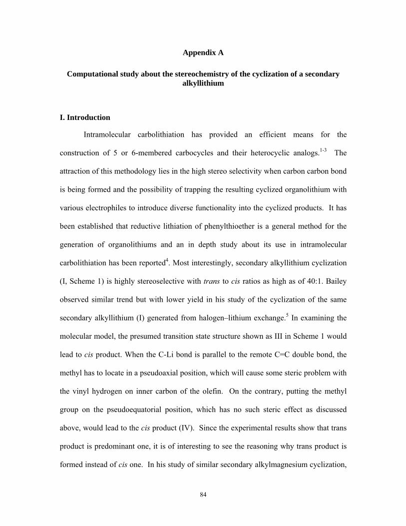
Appendix A
Computational study about the stereochemistry of the cyclization of a secondary alkyllithium
I. Introduction
Intramolecular carbolithiation has provided an efficient means for the
construction of 5 or 6-membered carbocycles and their heterocyclic analogs.1-3 The
attraction of this methodology lies in the high stereo selectivity when carbon carbon bond
is being formed and the possibility of trapping the resulting cyclized organolithium with
various electrophiles to introduce diverse functionality into the cyclized products. It has
been established that reductive lithiation of phenylthioether is a general method for the
generation of organolithiums and an in depth study about its use in intramolecular
carbolithiation has been reported4. Most interestingly, secondary alkyllithium cyclization
(I, Scheme 1) is highly stereoselective with trans to cis ratios as high as of 40:1. Bailey
observed similar trend but with lower yield in his study of the cyclization of the same
secondary alkyllithium (I) generated from halogen–lithium exchange.5 In examining the
molecular model, the presumed transition state structure shown as III in Scheme 1 would
lead to cis product. When the C-Li bond is parallel to the remote C=C double bond, the
methyl has to locate in a pseudoaxial position, which will cause some steric problem with
the vinyl hydrogen on inner carbon of the olefin. On the contrary, putting the methyl
group on the pseudoequatorial position, which has no such steric effect as discussed
above, would lead to the cis product (IV). Since the experimental results show that trans
product is predominant one, it is of interesting to see the reasoning why trans product is
formed instead of cis one. In his study of similar secondary alkylmagnesium cyclization,
84
Richey has proposed late transition state for his reaction to explain the high trans
selectivity in his reaction (trans/cis=10:1 in his case).6 However, it will be interested to
the synthetic community by doing calculations to explain the high trans selectivity in our
secondary alkyllithium cyclization. Since THF is used as the solvent for the reaction and
THF is known to be lithiophilic, it will be of interesting to examine the solvent effect.
Li
Li
(I) (II)
Li
Li
(III) (IV)
?
Scheme 1 Secondary alkyllithium Cyclization
II. Computational details
Calculations employing the B3LYP hybrid density functional method7-9 were
used to investigate the mechanisms of secondary cabanionic cyclization depicted in
Scheme 1. Geometry optimization of all reactants, products and transition states were
carried out using the 6-31+G(d) basis set10. Transition states were located using the
synchronous transit-guided quasi-Newton method of Schegal (QST3). Harmonic
frequency calculations were performed to establish the nature of each stationary point, to
calculate vibrational zero-point energy corrections, and to estimate free energies at the
reaction temperature -78 °C. All calculations were carried out using Gaussian 038.
The experiments were carried out in THF at -78 °C. Initially the solvent effect
was included through the polarizable continuum model (PCM)11,12. However, it is very
85

likely under these experimental conditions the Li+ ion is coordinated by THF molecules.
In order to investigate the importance of such coordination, calculations were also carried
out with inclusion of one or two THF molecules. Reactants, products and transition states
coordinated with one or two THF molecules are indicated by (thf) n (n=1, 2) in the figures
and tables.
III. Result and Discussion
The optimized minima and transition states are depicted schematically in Figures
1-3. Detailed structural parameters and energies for all the structures are reported in the
supporting information. The energies, ZPE’s, and free energy corrections of reactants,
transition states, and products are reported in tables 1-3.
The cyclohexane chair-like reactants are actually intermediates with the stability
derived from interaction of the Li+ with the π bond13,14. There are cis and trans
coordinated complexes. The reaction is racemic so both cis- and trans-complexes contain
mirror image structures. As can be seen from the data summarized in Figure 1, the
energies of cis reactant and trans reactant are very close with the cis-complex calculated
to be only 0.50 kcal/mol lower in energy. The greater stability of the cis complex appears
to be due to the less steric effects. There are a number of short, non-bonded hydrogen-
hydrogen and carbon-hydrogen interactions present in the trans intermediate complex
caused by the pseudoaxial methyl group.
The trans product is predicted to be 3.0 kcal/mol more stable than the cis product
as a consequence of steric effects of the cis product involving the methyl substituent and
the –CH2Li on the cyclopentane ring.
86
First, the theoretical study of gas phase pathways leading to cis and trans product
are conducted. The transition state search gives a chair-like transition state for the cis
reaction path. However, two transition states, one chair-like and the other twisted, are
found to lead to the trans product. In the twisted transition state, the methyl group
connected to C6 is in the equatorial plane, while in the chair-like transition state it is in
the pseudoaxial position. The twisted transition state is calculated to be about 0.18
kcal/mol lower in energy than the chair-like transition state for the trans pathway. The
transition state on the cis pathway is calculated to be 0.14 and 0.52 kcal/mol lower in
energy than the trans (twisted) and trans (chair-like) transition states, respectively.
Hence, the theoretical results for the gas phase pathways do not account for the highly
trans/cis ratio (40:1) observed in the experiments.
The solvent effect was included by performing single point calculations on the
optimized structures of the minima and transition states with PCM model of THF solvent.
The results show almost no changes in the reaction activation energies and can’t explain
the experiment results either.
We now consider the results of the calculations including explicit THF molecules.
Calculations about the effect of THF molecules on the reaction pathways are rare in the
literature. Piffl et al15 published their study on THF coordination with the sulfur-
stabilized allyllithium compounds both in NMR study and theoretical calculations. Our
study about the THF effect on the reaction pathways is shown in Figures 2 and 3, which
depicted the optimized structures of the THF-containing complexes as well as the total
energies with zero-point energy and free energy corrections. From these figures, it can be
seen that the C2-Li and C6-Li distances increase as a result of the coordination of THF.
87

The coordination of THF with Li+ weakens the interaction of Li with the π bond as well
as the carbon-lithium bond. A single THF molecule cause a stabilization of the chair-like
trans transition state relative to the twisted trans and cis transition states. In the chair-like
trans transition state the two rings lie roughly in the same plane, minimizing the H-H
non-bonded interactions. However, in the chair-like cis transition state and twisted trans
transition state, the dihedral angles of the THF ring and the transition state ring are about
150°. This flipping up of THF ring is due to the existence of the equatorial methyl group
connected to C5. With one THF molecule, the activation energy of the trans pathway is
2.65 kcal/mol below that in the cis pathway which would lead to over a 99% selectivity
for the trans product, well matching the experimental results.
The net binding energy of two THFs with reactant complex is calculated to be
about 18 kcal/mol. The energy of the trans reactant complex is now calculated to be
1.679 kcal/mol less stable than the cis complex. The activation energies of all three
pathways for two THF molecules are greater compared with one THF. However at
temperature -78°C, the ∆H for evaporation is -9.05 kcal/mol. It appears that the second
THF would prefer to stay in the solvent rather than coordinate with Li+ . Probably it is
rare for two THF molecules to coordinate with one Li+ at the same time. So this reaction
pathway will not be very likely happened in the real system.
IV. Conclusions
The lithiophilic solvent THF plays an important role in the high steroselectivity
reaction of secondary alkyllithium cyclization. Steric effects have been shown to have a
major influence on the selectivity of this reaction. Quantum mechanical calculations
about the coordination of one THF molecule with Li+ can be used to explain the
88

experimental results very well. THF is a principal member of the class of dipolar aprotic
solvent, which serves as ideal media for a variety of important chemical reactions. The
strong interaction of THF with Li+ and the steric effect caused by THF is believed to
increase the selectivity of the cyclization reaction and even change the reaction pathway.
89

References
(1) Bailey, W. F. and Ovaska, T. V. In Advances in Detailed Reaction Mechanisms; Coxon, J. M., Ed.; JAI Press: Greenwich, CT, 1994; Vol. 3; pp 251.
(2) Mealy, M. J. and Bailey, W. F. J. Organomet. Chem. 2002, 646, 59.
(3) Clayden, J. Organolithiums: Selectivity for Synthesis; Pergamon Press: New York, NY, 2002.
(4) Deng, K., Bensari, A. and Cohen, T. J. Am. Chem. Soc. 2002, 124, 12106.
(5) Bailey, W. F., Nurmi, T. T., Patricia, J. J. and Wang, W. J. Am. Chem. Soc. 1987, 2441.
(6) Walter, C. K., Rees, T. C. and Richey, H. G. Tetrahedron Lett. 1971, 3455.
(7) Becke, A. D. J. Chem. Phys. 1993, 98, 5648.
(8) M. J. Frisch, G. W. T., H. B. Schlegel, G. E. Scuseria,, M. A. Robb, J. R. C., J. A. Montgomery, Jr., T. Vreven,, K. N. Kudin, J. C. B., J. M. Millam, S. S. Iyengar, J. Tomasi,, V. Barone, B. M., M. Cossi, G. Scalmani, N. Rega,, G. A. Petersson, H. N., M. Hada, M. Ehara, K. Toyota,, R. Fukuda, J. H., M. Ishida, T. Nakajima, Y. Honda, O. Kitao,, H. Nakai, M. K., X. Li, J. E. Knox, H. P. Hratchian, J. B. Cross,, C. Adamo, J. J., R. Gomperts, R. E. Stratmann, O. Yazyev,, A. J. Austin, R. C., C. Pomelli, J. W. Ochterski, P. Y. Ayala,, K. Morokuma, G. A. V., P. Salvador, J. J. Dannenberg,, V. G. Zakrzewski, S. D., A. D. Daniels, M. C. Strain,, O. Farkas, D. K. M., A. D. Rabuck, K. Raghavachari,, J. B. Foresman, J. V. O., Q. Cui, A. G. Baboul, S. Clifford,, J. Cioslowski, B. B. S., G. Liu, A. Liashenko, P. Piskorz,, I. Komaromi, R. L. M., D. J. Fox, T. Keith, M. A. Al-Laham,, C. Y. Peng, A. N., M. Challacombe, P. M. W. Gill, and B. Johnson, W. C., M. W. Wong, C. Gonzalez, and J. A. Pople. Gaussian 03, Revision C.01. In Gaussian, Inc., Wallingford CT, 2004.
(9) Lee, C., Yang, W. and Parr, R. G. Phys. Rev. B, 1988, 37, 785789.
(10) Hehre, W. J., Ditchfield, R. and Pople, J. A. J. Chem. Phys. 1972, 56, 2257.
(11) Tomasi, J., Cammi, R. and Mennucci, B. Int. J. Quantum Chem. 1999, 75, 783.
(12) Cossi, M., Barone, V., Cammi, R. and Tomasi, J. Chem. Phys. Lett. 1996, 255, 327.
90

(13) Bailey, W. F., Khanolkar, A. D., Gavaskar, K., Ovaska, T. V., Rossi, K., Thiel, Y. and Wiberg, K. B. J. Am. Chem. Soc. 1991, 113, 5720.
(14) Wu, Y. D. and Houk, K. N. J. Am. Chem. Soc. 1987, 109, 908.
(15) Piffl, M., Weston, J., Gunther, W. and Anders, E. J. Org. Chem. 2000, 65, 5942.
91
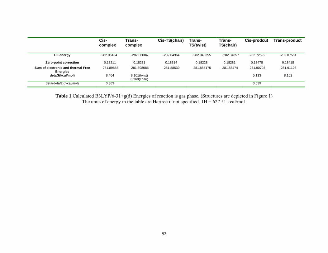
Cis-complex
Trans-complex
Cis-TS(chair) Trans-TS(twist)
Trans-TS(chair)
Cis-prodcut Trans-product
HF energy -282.06134 -282.06084 -282.04964 -282.048355 -282.04857 -282.72592 -282.07551
Zero-point correction 0.18211
0.18231 0.18314 0.18228 0.18281 0.18478 0.18418Sum of electronic and thermal Free
Energies -281.89888 -281.898085 -281.88539 -281.885175 -281.88474 -281.90703 -281.91108
detaG(kcal/mol) 8.464 8.101(twist)8.369(chair)
5.113 8.152
deta(detaG)(/kcal/mol) 0.363 3.039
Table 1 Calculated B3LYP/6-31+g(d) Energies of reaction is gas phase. (Structures are depicted in Figure 1)
The units of energy in the table are Hartree if not specified. 1H = 627.51 kcal/mol.
92
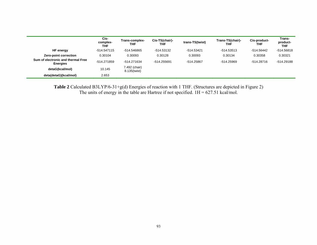
Cis-
complex-THF
Trans-complex-THF
Cis-TS(chair)-THF trans-TS(twist) Trans-TS(chair)-
THF Cis-product-
THF Trans-
product-THF
HF energy -514.547115
-514.546865 -514.53132 -514.53421 -514.53513 -514.56442 -514.56818Zero-point correction 0.30104 0.30093 0.30128 0.30093 0.30134 0.30358 0.30321
Sum of electronic and thermal Free Energies -514.271859 -514.271634 -514.255691 -514.25867 -514.25969 -514.28716 -514.29188
detaG(kcal/mol) 10.145 7.492 (chair) 8.135(twist)
deta(detaG)(kcal/mol) 2.653
Table 2 Calculated B3LYP/6-31+g(d) Energies of reaction with 1 THF. (Structures are depicted in Figure 2)
The units of energy in the table are Hartree if not specified. 1H = 627.51 kcal/mol.
93
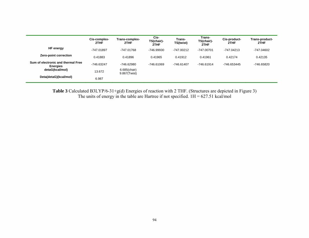
Cis-complex-2THF
Trans-complex-2THF
Cis-TS(chair)-
2THF
Trans-TS(twist)
Trans-TS(chair)-
2THF
Cis-product-2THF
Trans-product-2THF
HF energy -747.01897
-747.01768 -746.99930 -747.00212 -747.00701 -747.04213 -747.04602
Zero-point correction 0.41883 0.41896 0.41965 0.41912 0.41961 0.42174 0.42135
Sum of electronic and thermal Free Energies -746.63247 -746.62980 -746.61069 -746.61407 -746.61914 -746.653445 -746.65820
detaG(kcal/mol) 13.672 6.685(chair)
9.867(Twist) Deta(detaG)(kcal/mol)
6.987
Table 3 Calculated B3LYP/6-31+g(d) Energies of reaction with 2 THF. (Structures are depicted in Figure 3)
The units of energy in the table are Hartree if not specified. 1H = 627.51 kcal/mol
94
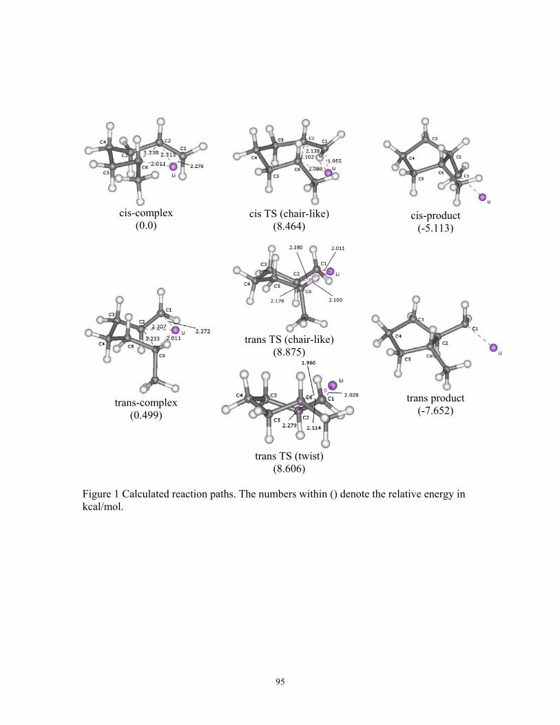
cis-complex
(0.0)
cis TS (chair-like)
(8.464)
cis-product
(-5.113)
trans TS (chair-like)
(8.875)
trans-complex
(0.499)
trans TS (twist) (8.606)
trans product (-7.652)
Figure 1 Calculated reaction paths. The numbers within () denote the relative energy in kcal/mol.
95

cis-complex with 1THF
(0.0)
cis TS with THF (chair-like) (10.145)
cis-product-with 1THF
(-9.603)
trans TS with THF(chair-like)
(7.639)
trans-complex with 1THF
(0.141)
trans TS with THF(twist)
(8.2743)
trans-product with 1THF (-12.563)
Figure 2 Calculated reaction paths with 1 explicit THF molecule. The numbers within ( ) denote the relative energy in kcal/mol
96

cis-complex with 2THF
(0.0)
cis TS with 2THF(chair)
(13.672)
cis product (-13.160)
trans TS with 2THF(chair)
(8.365)
trans-complex with 2THF
(1.679)
trans TS with 2THF(twist)
(11.546)
trans product
(-16.143)
Figure 3 Calculated reaction paths with two explicit THF molecules. The numbers within () denote the relative energy in kcal/mol.
97
Appendix B
Theoretical characterization of the (H2O)21 cluster
Jun Cui, Hanbin Liu, and Kenneth D. Jordan*
Department of Chemistry and Center for Molecular and Materials Simulations
University of Pittsburgh
Pittsburgh, PA 15260
Abstract: In this paper, we examine theoretically the structures and energies of selected
low energy isomers of (H2O)20 and (H2O)21, with particular attention paid to isomers
derived from water dodecahedron. Results are reported for the Becke3LYP density
functional and the RI-MP2 electronic structure methods, as well as for several water
models. The calculations reveal that the global minimum structure of (H2O)21 is a water
dodecahedron with an interior water molecule engaged in four hydrogen bonds. This
indicates that the excess proton is not “driving” the high stability of the magic number
H+(H2O)21 cluster, the global minimum of which is also derived from the water
dodecahedron and has interior water molecule.
98
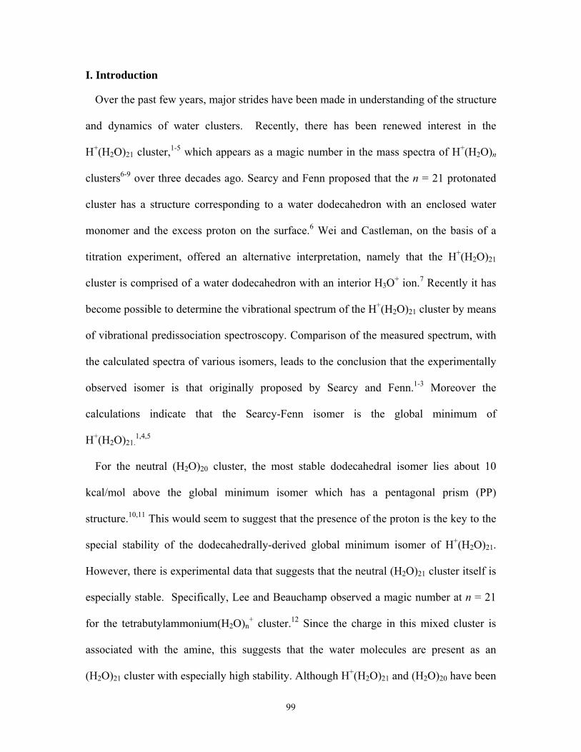
I. Introduction
Over the past few years, major strides have been made in understanding of the structure
and dynamics of water clusters. Recently, there has been renewed interest in the
H+(H2O)21 cluster,1-5 which appears as a magic number in the mass spectra of H+(H2O)n
clusters6-9 over three decades ago. Searcy and Fenn proposed that the n = 21 protonated
cluster has a structure corresponding to a water dodecahedron with an enclosed water
monomer and the excess proton on the surface.6 Wei and Castleman, on the basis of a
titration experiment, offered an alternative interpretation, namely that the H+(H2O)21
cluster is comprised of a water dodecahedron with an interior H3O+ ion.7 Recently it has
become possible to determine the vibrational spectrum of the H+(H2O)21 cluster by means
of vibrational predissociation spectroscopy. Comparison of the measured spectrum, with
the calculated spectra of various isomers, leads to the conclusion that the experimentally
observed isomer is that originally proposed by Searcy and Fenn.1-3 Moreover the
calculations indicate that the Searcy-Fenn isomer is the global minimum of
H+(H2O)21.1,4,5
For the neutral (H2O)20 cluster, the most stable dodecahedral isomer lies about 10
kcal/mol above the global minimum isomer which has a pentagonal prism (PP)
structure.10,11 This would seem to suggest that the presence of the proton is the key to the
special stability of the dodecahedrally-derived global minimum isomer of H+(H2O)21.
However, there is experimental data that suggests that the neutral (H2O)21 cluster itself is
especially stable. Specifically, Lee and Beauchamp observed a magic number at n = 21
for the tetrabutylammonium(H2O)n+ cluster.12 Since the charge in this mixed cluster is
associated with the amine, this suggests that the water molecules are present as an
(H2O)21 cluster with especially high stability. Although H+(H2O)21 and (H2O)20 have been
99
the subject of numerous theoretical studies, the neutral (H2O)21 cluster has received much
less attention. Wales and Hodges have characterized (H2O)21 using the TIP4P water
model13 and reported that the global minimum has a “flat” structure comprised of fused
four- and five- membered rings,10 and hereafter referred to as TIP4P-gm(21).
In this paper, we examine theoretically the structures and energies of selected low
energy isomers of (H2O)20 and (H2O)21, with particular attention paid to isomers derived
from water dodecahedron. Results are reported for the Becke3LYP density functional14-16
and the resolvent of the identity second order Møller-Plesset perturbation Theory (RI-
MP2) electronic structure methods,17 as well as for the TIP4P effective two-body model
potential, and for the Dang-Chang,18 AMOEBA,19 and TTM2-F20 polarizable water
models.
II. Computational details
The Becke3LYP calculations were performed with both the 6-31+G(d) and aug-cc-
pVDZ21,22 basis sets, and the RI-MP2 calculations were performed using both the aug-cc-
pVDZ and aug-cc-pVTZ(-f)21,22 basis sets. The –f in the latter case indicates that the f
functions on the O atoms and the d functions on the H atoms that would be present in the
full aug-cc-pVTZ basis set have been omitted. The RI-MP2 calculations with the aug-cc-
pVTZ(-f) basis set were carried out using the RI-MP2/aug-cc-pVDZ optimized
geometries. The Becke3LYP and RI-MP2 calculations were carried out using Gaussian
0316 and Turbomole,23,24 respectively. The calculations with the TIP4P and Dang-Chang,
AMOEBA force fields were carried out using the Tinker program,19,25-27 and the
calculations with the TTM2-F force field were carried out using the Occident program
from Xantheas group.20
100
Clusters of the size of (H2O)20 and (H2O)21 have a very large number of low-lying local
minima, making location of the global minimum especially challenging.10 In this work
we adopted several strategies in searching for low energy minima. First, we selected low-
energy structures from the Cambridge Cluster Database10 which were located by means
of the basin hopping Monte Carlo procedure28 and using the TIP4P water model. In the
case of (H2O)21, we also built structures by adding a water molecule in the interior of the
(H2O)20 dodecahedron. Since there are multiple isomers of this type, these structures were
used to initialize eigenmode-following searches29-31 for other minima and as initial
structures for use in simulated annealing calculations, carried out with molecular
dynamics simulations and the AMOEBA force field. For (H2O)20, we also examined
structures formed by removing one of the surface water molecule from the most stable
dodecahedrally derived form of (H2O)21. The lowest energy structures thus located were
used to initiate geometry optimizations with the various force fields as well as with the
Becke3LYP and RI-MP2 electronic structure methods.
III. Results and Discussion
In discussing the results for (H2O)21, we focus primarily on the two isomers denoted
TIP4P-gm(21) and DD(20,1) and depicted in Figure 1. The former is the global minimum
located by Wales and Hodges using the TIP4P model, and the latter denotes a distorted
dodecahedron with an interior water molecule engaged in four hydrogen bonds. The
DD(20,1) isomer has a structure similar to the global minimum of (H2O)21 except for the
absence of the excess proton in H+(H2O)21. Figure 2 reports for the TIP4P-gm(21) and
DD(20,1) isomers of (H2O)21 as well as of four forms of (H2O)20 the binding energies.
The Becke3LYP/aug-cc-pVDZ and RI-MP2/aug-cc-pVDZ calculations place the
101
DD(20,1) isomer energetically below the TIP4P-gm(21) isomer by 6.7 and 4.2 kcal/mol,
respectively. The energy difference between the two isomers is 4.6 kcal/mol at the RI-
MP2/aug-cc-pVTZ(-f) level. Inclusion of corrections for vibrational zero-point energy
(estimated at the Becke3LYP/6-31+G(d) level) further stablizes the DD(20,1) structure
over the TIP4P-gm(21) isomer by 1.2 kcal/mol.
At the RI-MP2/aug-cc-pVDZ level of theory the counterpoise correction for basis set
superposition error (BSSE) is 43.1 kcal/mol for both the DD(20,1) and TIP4P-gm(21)
isomers. The corresponding counterpoise corrections are -28.1 and -27.5 kcal/mol at the
RI-MP2/aug-cc-PVTZ(-f) level. Thus, while the BSSE corrections are large for the basis
sets employed, they are nearly identical for the two isomers, for both basis sets
considered. As a result, we conclude that the DD(20,1) isomer would be about 5 kcal/mol
more stable (before ZPE correction) than the TIP4P-gm(21) isomer in the complete basis
set limit.
The TTM2-F and AMOEBA polarizable models favor the DD(20,1) isomer by 1.1 and
4.0 kcal/mol respectively. On the other hand, the TIP4P and DC models both predict the
TIP4P-gm(21) isomer to be slightly more stable than the DD(20,1) isomer. Thus, it
appears that in a model potential approach both distributed polarizable sites and a
realistic description of the electrostatics are required in order to properly describe the
energy difference between the TIP4P-gm(21) and DD(20,1) isomers of (H2O)21.
For (H2O)20, results are reported in Figure 2 for the “perfect” dodecahedron [PD(20)],
the pentagonal prism [PP(20)], and the DD(19,1) isomer, which is formed by removing a
water from the surface of DD(20,1) and allowing for geometrical relaxation. The
structures of the PD(20), PP(20), and DD(19,1) isomers are depicted on Figure 1. Figure
102
2 also reports energies for a structure designated DD(20,0), formed by removing the
interior water molecule from DD(20,1), without allowing relaxation of the geometry. As
seen from Figure 2, for (H2O)20, PP(20) is the global minimum at all levels of theory
considered, although the energy gap between PP(20) and DD(19,1) is only 1.3 kcal/mol
at the RI-MP2/aug-cc-pVTZ(-f) level. The DD(20,0) species is calculated to be less
stable by 5-15 kcal/mol, depending on the theoretical method employed, than the PD(20)
isomer. This represents the energetic cost of distorting the (H2O)20 dodecahedron into the
structure it has in the DD(20,1) isomer. The DD(20,1) species is 26-35 kcal/mol more
stable than the DD(20,0) species, for the theoretical methods considered. Again, the
energy difference obtained using the TTM2-F and AMOEBA models are in fairly good
agreement with the RI-MP2/aug-cc-pVTZ(-f) results.
There are siginificant differences between the relative energies, and those from the
AMOEBA and RI-MP2 calculations. This may be a consequence of the well-known
inadequency of the density functional methods for describing dispersion interactions.32
IV. Conclusions
The present study provides evidence that the DD(20,1) isomer of (H2O)21, which
consists of a distorted water dodecahedron with an interior water engaged in four H-
bonds, is significantly more stable than the TIP4P-gm(21) isomer, which is lowest energy
isomer of (H2O)21 located with the TIP4P water model. At the RI-MP2/aug-cc-pVTZ(-f)
level the DD(20,1) isomer is calculated to be 22.9 kcal/mol more stable than the global
minimum of (H2O)20. This is an unusually large difference in stability for two adjacent
(i.e., n and n+1) water clusters and is consistent with the experiments of Lee et al., which
suggested an unusually high stability of (H2O)21. The high stability of the DD(20,1)
103
isomer derives from the presence of the four strong H-bonds involving the interior water
molecule. These results also indicate that the high stability of the Searcy-Fenn form of
H+(H2O)21 is due primarily to the strong H-bonds involving the interior water monomer
rather than to the excess proton.
Surprisingly, it is found that Dang-Chang polarizable water model fails to predict that
DD(20,1) isomer is more stable than TIP4P-gm(21). The TTM2-F and AMOEBA water
models, which employ distributed polarizable sites, do predict the DD(20,1) isomer to be
more stable than the TIP4P-gm(21) isomer. Of these two models, the AMOEBA model,
which also employs distributed multipoles, gives an energy difference closer to the RI-
MP2 results than does the TTM2-F model. Thus it appears that the use of both distributed
multipoles and distributed polarizable sites is necessary to provide a realistic description
of (H2O)21.
For (H2O)20 the RI-MP2 calculations predict that the DD(19, 1) isomer to be only 1.3
kcal/mol less stable than the PP(20) global minimum isomer. Interestingly, several
papers, discussing various type of isomers of (H2O)20, have not mentioned this
species.11,33,34
The DD(20,1) isomer investigated here is calculated to have a dipole moment of 3.00
D. As a result, this isomer should form a stable dipole bound anion, which would allow
access to the neutral DD(20,1) form of (H2O)21 via photo-detachment of the anion.
Acknowledgements: This research was carried out with the support of the National
Science Foundation.
104
References
(1) Shin, J. W.; Hammer, N. I.; Diken, E. G.; Johnson, M. A.; Walters, R. S.; Jaeger,
T. D.; Duncan, M. A.; Christie, R. A.; Jordan, K. D. Science 2004, 304, 1137.
(2) Miyazaki, M.; Fujii, A.; Ebata, T.; Mikami, N. Science 2004, 304, 1134.
(3) Wu, C.-C.; Lin, C.-K.; Chang, H.-C.; Jiang, J.-C.; Kuo, J.-L.; Klein, M. L. J.
Chem. Phys. 2005, 122, 074315.
(4) Kuo, J.-L.; Klein, M. L. J. Chem. Phys. 2005, 122, 024516.
(5) James, T.; Wales, D. J. J. Chem. Phys. 2005, in press.
(6) Searcy, J. Q.; Fenn, J. B. J. Chem. Phys. 1974, 61, 5282.
(7) Wei, S.; Shi, Z.; Castleman, A. W.; Jr. J. Chem. Phys. 1991, 94, 3268.
(8) Lee, S. W.; Cox, H.; Goddard, W. A.; Beauchamp, J. L. J. Am. Chem. Soc. 2000,
122, 9201.
(9) Niedner-Schatteburg, G.; Bondybey, V. E. Chem. Rev. 2000, 100, 4059
(10) Wales, D. J.; Hodges, M. P. Chem. Phys. Lett. 1998, 286, 65.
(11) Fanourgakis, G. S.; Apra, E.; Xantheas, S. S. J. Chem. Phys. 2004, 121, 2655.
(12) Lee, S. W.; Freivogel, P.; Schindler, T.; Beauchamp, J. L. J. Am. Chem. Soc.
1998, 120, 11758.
(13) Jorgensen, W. L.; Chandrasekhar, J.; Madura, J. D.; Impey, R. W.; Klein, M. L. J.
Chem. Phys. 1983, 79, 926.
105
(14) Becke, A. D. J. Chem. Phys. 1993, 98, 5648.
(15) Lee, C.; Yang, W.; Parr, R. G. Phys. Rev. B 1988, 37, 785–789.
(16) M. J. Frisch, G. W. T., H. B. Schlegel, G. E. Scuseria,; M. A. Robb, J. R. C., J. A.
Montgomery, Jr., T. Vreven,; K. N. Kudin, J. C. B., J. M. Millam, S. S. Iyengar, J.
Tomasi,; V. Barone, B. M., M. Cossi, G. Scalmani, N. Rega,; G. A. Petersson, H. N., M.
Hada, M. Ehara, K. Toyota,; R. Fukuda, J. H., M. Ishida, T. Nakajima, Y. Honda, O.
Kitao,; H. Nakai, M. K., X. Li, J. E. Knox, H. P. Hratchian, J. B. Cross,; C. Adamo, J. J.,
R. Gomperts, R. E. Stratmann, O. Yazyev,; A. J. Austin, R. C., C. Pomelli, J. W.
Ochterski, P. Y. Ayala,; K. Morokuma, G. A. V., P. Salvador, J. J. Dannenberg,; V. G.
Zakrzewski, S. D., A. D. Daniels, M. C. Strain,; O. Farkas, D. K. M., A. D. Rabuck, K.
Raghavachari,; J. B. Foresman, J. V. O., Q. Cui, A. G. Baboul, S. Clifford,; J.
Cioslowski, B. B. S., G. Liu, A. Liashenko, P. Piskorz,; I. Komaromi, R. L. M., D. J. Fox,
T. Keith, M. A. Al-Laham,; C. Y. Peng, A. N., M. Challacombe, P. M. W. Gill,; B.
Johnson, W. C., M. W. Wong, C. Gonzalez, and J. A. Pople. Gaussian, Inc., Wallingford
CT 2004.
(17) Feyereisen, M.; Fitzgerald, G.; Komornicki, A. Chem. Phys. Lett. 1993, 208, 359.
(18) Dang, L. X.; Chang, T.-M. J. Chem. Phys. 1997, 106, 8149.
(19) Ren, P. Y.; Ponder, J. W. J. Phys. Chem. B 2003, 107, 5933.
(20) Burnham, C. J.; Xantheas, S. S. J. Chem. Phys. 2002, 116, 5115.
(21) Dunning, T. H.; Jr. J. Chem. Phys. 1989, 90, 1007.
(22) Kendall, R. A.; Dunning, T. H.; Harrison, R. J. J. Chem. Phys. 1992, 96, 6796.
106

(23) Treutler, O.; Ahlrichs, R. J. Chem. Phys. 1995, 102, 346.
(24) Von Arnim, M.; Ahlrichs, R. J. Comput. Chem. 1998, 19, 1746.
(25) Ren, P. Y.; Ponder, J. W. J. Comput. Chem. 2002, 23, 1497.
(26) Pappu, R. V.; Hart, R. K.; Ponder, J. W. J. Phys. Chem. B 1998, 102, 9725.
(27) Hodsdon, M. E.; Ponder, J. W.; Cistola, D. P. J. Mol. Biol. 1996, 264, 585.
(28) Scheraga, Z. L. H. A. Proc. Nat. Acad. Sci. USA 1987, 84, 6611.
(29) Simons, J.; Jerrgensen, P.; Taylor, H.; Orment, J. J. Phys. Chem. 1983, 87, 2745.
(30) Banerjee, A.; Adams, N.; Simons, J.; Shepard, R. J. Phys. Chem. 1985, 89, 52.
(31) Cerjan, C. J.; Miller, W. H. J. Chem. Phys. 1981, 75, 2800.
(32) Boys, S. F.; Bernardi, F. Mol. Phys. 1970, 19, 553.
(33) Tsai, C. J.; Jordan, K. D. J. Phys. Chem. 1993, 97, 5208.
(34) Sremaniak, L. S.; Perera, L.; Berkowitz, M. L. J. Chem. Phys. 1996, 105, 3715.
107
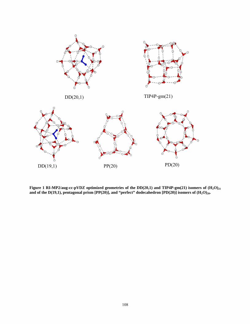
TIP4P-gm(21) DD(20,1)
PD(20) DD(19,1) PP(20)
Figure 1 RI-MP2/aug-cc-pVDZ optimized geometries of the DD(20,1) and TIP4P-gm(21) isomers of (H2O)21 and of the D(19,1), pentagonal prism [PP(20)], and “perfect” dodecahedron [PD(20)] isomers of (H2O)20.
108
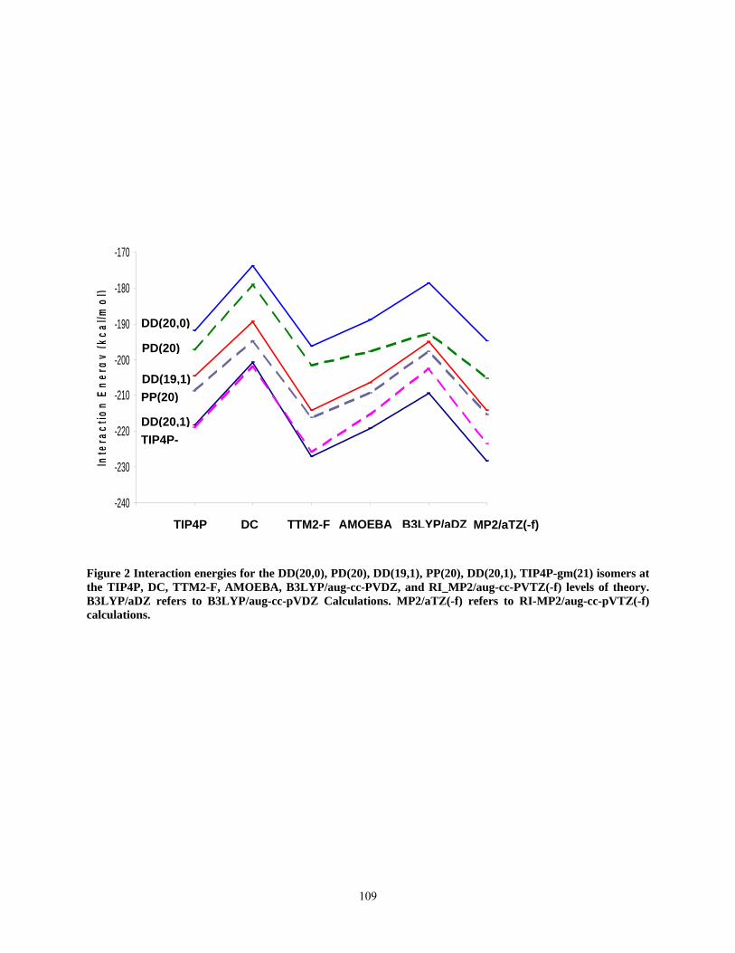
-240
-230
-220
-210
-200
-190
-180
-170
Inte
ract
ion
Ener
gy(k
cal/m
ol)
TIP4P-DD(20,1)
PP(20) DD(19,1)
PD(20)
DD(20,0)
AMOEBA B3LYP/aDZTIP4P DC TTM2-F MP2/aTZ(-f)
Figure 2 Interaction energies for the DD(20,0), PD(20), DD(19,1), PP(20), DD(20,1), TIP4P-gm(21) isomers at the TIP4P, DC, TTM2-F, AMOEBA, B3LYP/aug-cc-PVDZ, and RI_MP2/aug-cc-PVTZ(-f) levels of theory. B3LYP/aDZ refers to B3LYP/aug-cc-pVDZ Calculations. MP2/aTZ(-f) refers to RI-MP2/aug-cc-pVTZ(-f) calculations.
109