Visualization Advanced Algorithms

(Ch. 9)

2012-10-01

Overview in data space – Taxonomy Advanced visual mappings Advanced algorithms

Outline

…is about mapping data to visual form It requires understanding of the nature of the data to be visualized.

Advanced visualization….

How can data be characterized?

Attributes (properties, variables) Type Dimensionality

Represented over a certain Domain

Dimensionality Type Regularity

Taxonomy

Attribute - Types – Nominal (label names, qualities)

– Ordinal (rank , position)

– Numerical Cardinal (can be counted)

Discrete quantities/intervals (integer)

Continuous quantities/intervals (rational numbers)

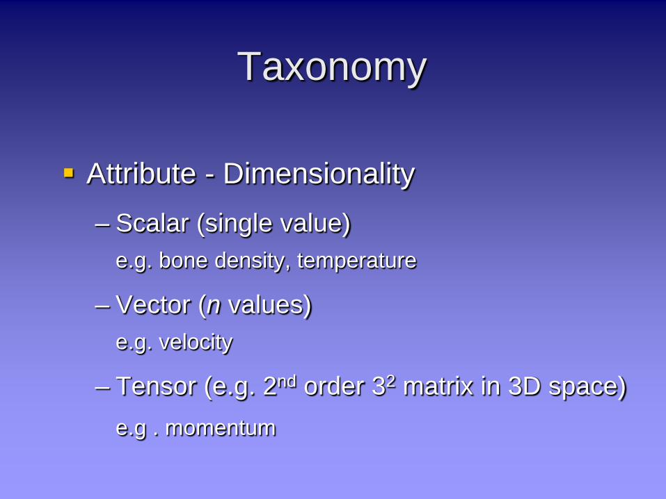
Taxonomy

Attribute - Dimensionality – Scalar (single value)

e.g. bone density, temperature

– Vector (n values) e.g. velocity

– Tensor (e.g. 2nd order 32 matrix in 3D space) e.g . momentum

Taxonomy Dimensionality of domain

– 1D: e.g. stock value over time

– 2D: e.g. light intensity across an area-sensor

– 3D: e.g. bone density in an anatomic specimen

– 4D: e.g. temporal change of a 3D temperature distribution

Domain types – Spatial, Temporal, Frequency

Domain regularity – Curvature (rectilinear, curvilinear grid over a surface)

– Continuous, discrete

Visual Mapping How can attributes of certain type and dimensionality

which are represented in domains of any dimensionality be mapped upon visual structure?

Visual structures have different properties – Spatial position, size, orientation and shape

– Color and gradient

– Texture

– Transparency

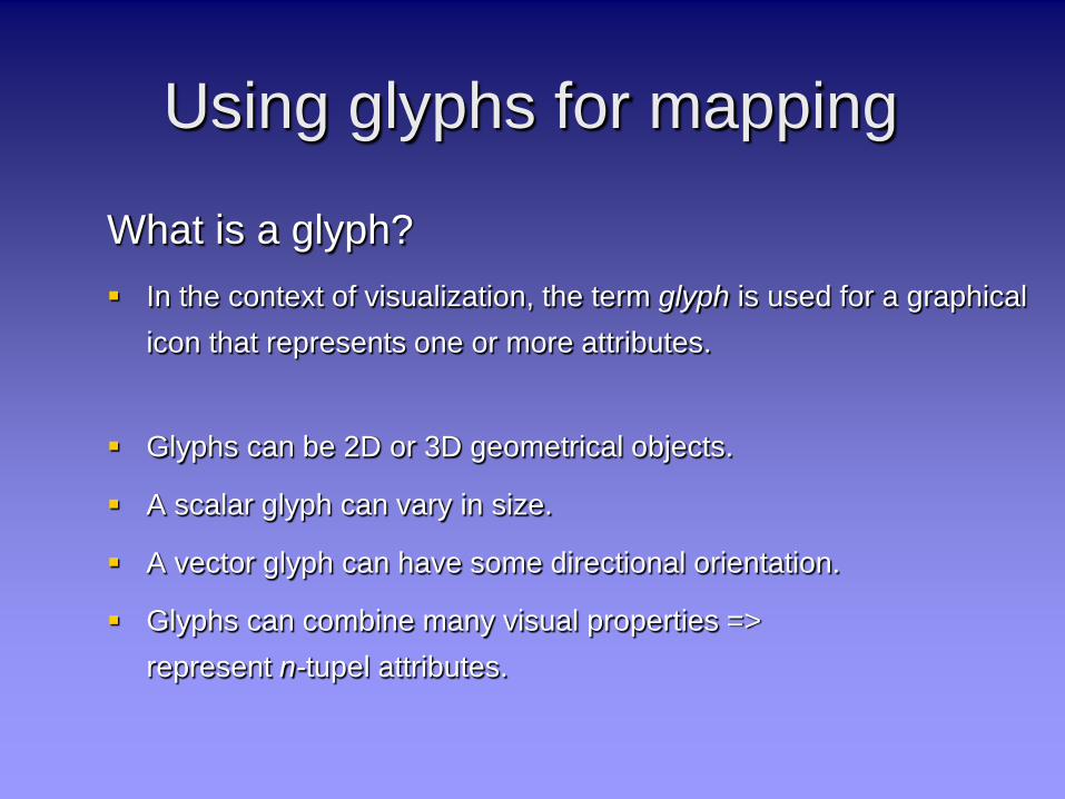
Using glyphs for mapping

What is a glyph? In the context of visualization, the term glyph is used for a graphical

icon that represents one or more attributes.

Glyphs can be 2D or 3D geometrical objects.

A scalar glyph can vary in size.

A vector glyph can have some directional orientation.

Glyphs can combine many visual properties => represent n-tupel attributes.

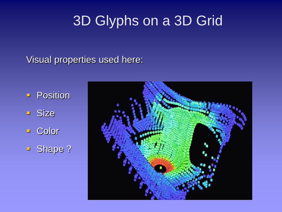
3D Glyphs on a 3D Grid

Visual properties used here:

Position

Size

Color

Shape ?

For scientific visualization of some entity E: Suppose attributes are quantities Attributes dimension is 1 => scalar S Defined on a n-dimensional domain: Ed

(n)S

Taxonomy Example application Vis. Technique/Mapping

E1S e.g. any function of time Line graph

E2S Meteorology, Photography Contour lines

Medicine Image display

Surface view

Mapping techniques for scalar data

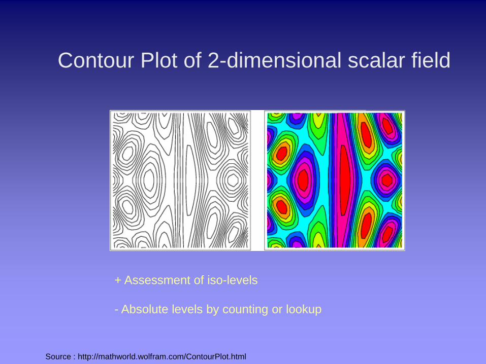
Source : http://mathworld.wolfram.com/ContourPlot.html

Contour Plot of 2-dimensional scalar field

+ Assessment of iso-levels - Absolute levels by counting or lookup

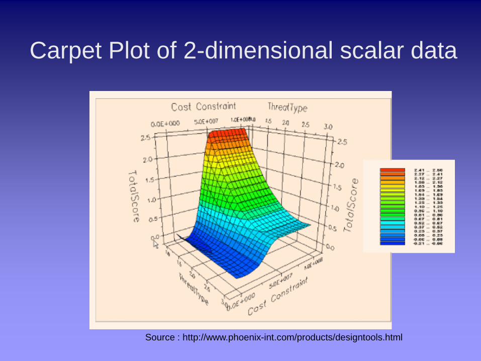
Source : http://www.phoenix-int.com/products/designtools.html

Carpet Plot of 2-dimensional scalar data

Taxonomy Example application Vis. Technique/Mapping E2

nS Multi-channel 2d sensor data Height-field plots w. color Geography (elevation, color) 2D scatter plots with glyphs Medical sciences E3

S Medical sciences Iso-surfaces+surface Physics, Chemistry rendering Geo-Sciences Direct volume rendering Slicing, Cutting E3

nS Medical sciences same as E3nS in combination

FE analysis with colours an glyphs Geo-Sciences

Em

nS Physics projection to lower dimensions Computer Science animation

Mapping techniques for scalar data

http://www.siggraph.org/education/materials/HyperVis/vised/VisTech/Techniques/sndaheightfield.html

Height-Field Plot (multivariate 2D scalar field)

Elevation model. Hue indicates type of vegetation

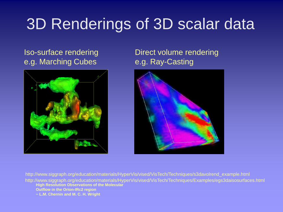
Iso-surface rendering e.g. Marching Cubes

High Resolution Observations of the Molecular Outflow in the Orion-IRc2 region ~ L.M. Chernin and M. C. H. Wright

http://www.siggraph.org/education/materials/HyperVis/vised/VisTech/Techniques/Examples/egs3daisosurfaces.html

Direct volume rendering e.g. Ray-Casting

3D Renderings of 3D scalar data

http://www.siggraph.org/education/materials/HyperVis/vised/VisTech/Techniques/s3davolrend_example.html

3D scalar field rendering - Dividing Cubes

Idea: Draw an implicit model by splatting all voxels classified as object. • Point based rendering technique, is fast • No connectivity/topology information needed • Save only object-voxels • Solid surface appears only if point cloud dense enough, otherwise ….

Voxel splatting artifacts

Voxel Splatting Artifacts: Solution: - “Fat splats”

- “Refined voxel models” (e.g. dividing cubes)

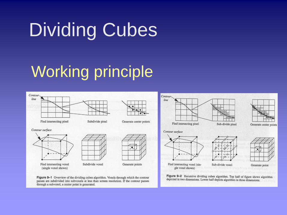
Dividing Cubes

Working principle

Issues in regard to 3D techniques

Computer screen is a 2D display surface -> 3D representation must be projected to eliminate z Problems: • Occlusion • Ambiguities (front or back?) • Distortion (if perspective projection is used)

One simple solution

• Show a “2D subset” of the data in context Depending on how the ”2D subset” is defined different names are used for this technique: ”Slicing” ”Cutting” ”Probing”

http://www.mathworks.com/access/helpdesk/help/techdoc/ref/slice.shtml

Slicing – 2D base plane in original domain

http://www.vis.uni-stuttgart.de/eng/research/fields/current/volclipping/

Cutting – Curved surface, cube surface

By Daniel Weiskopf

Probing

• Sampling one dataset with a set of points • Most general • Arbitrary probe shapes and topologies • Re-sampling -> aliasing/filtering • Display of probe data depends on probe topology and attribute types

Probing

Textbook page 337

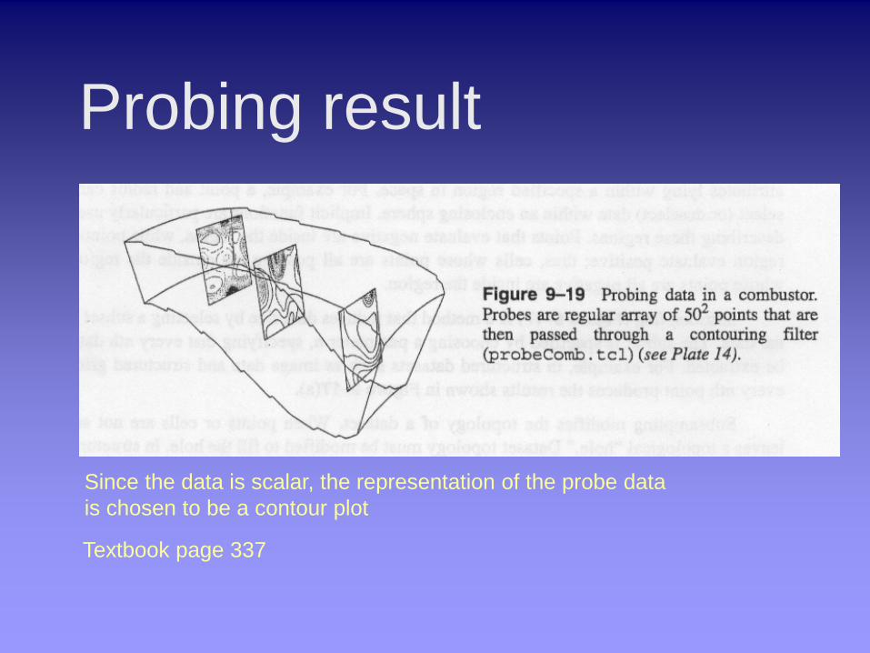
Probing result

Textbook page 337

Since the data is scalar, the representation of the probe data is chosen to be a contour plot

Cutting, slicing, probing

When probing scalar fields, the representation of the re-sampled data depends on the attributes of the original domain Vector data on a surface probe can be used to e.g. warp the surface -> carpet plot OBS: Ambiguity problem. Can be difficult to interpret if probe surface is curved !!! Is 3D shape due to vector-warp or due to curved probe?

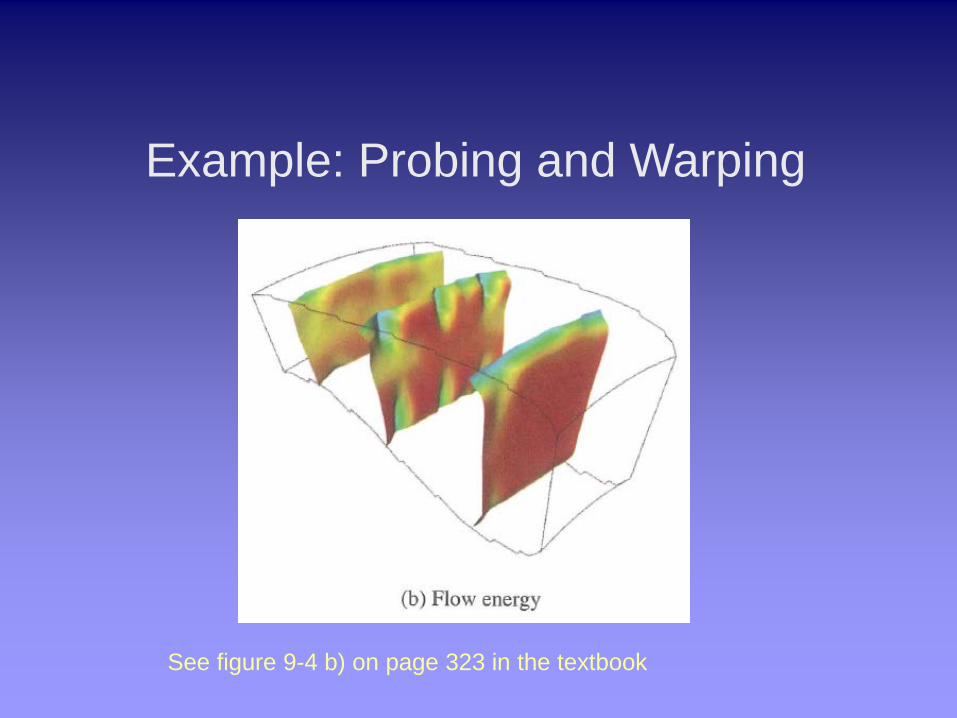
Example: Probing and Warping

See figure 9-4 b) on page 323 in the textbook

Mapping techniques for vector/tensor data

For scientific visualization of some entity E: Suppose attributes are n-vectors or n x n-tensors Defined on a n-dimensional domain: Ed

Vn or EdTn;n

Taxonomy Example application Vis. Technique/Mapping E2

V2 Physics, CFD, Meteorology Arrow plots E2

V2 Oceanography Particle tracing Stream lines E2;t

V2 “ Streak lines E2;t

V3 “ See E2V2

E2;tV3 Hedgehogs

Particle animation

Mapping techniques for vector/tensor data

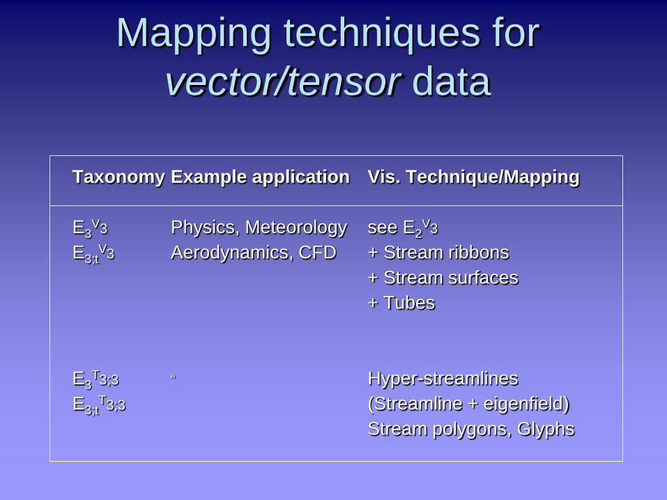
Taxonomy Example application Vis. Technique/Mapping E3

V3 Physics, Meteorology see E2V3

E3;tV3 Aerodynamics, CFD + Stream ribbons

+ Stream surfaces + Tubes E3

T3;3 “ Hyper-streamlines E3;t

T3;3 (Streamline + eigenfield) Stream polygons, Glyphs

Hedgehogs Arrow-Plots Streamlines Streaklines Particle tracing / animation Stream Ribbons Stream Surfaces (Stream Polygons)

Drawing techniques for vector fields

Hedgehogs

http://www.cc.gatech.edu/gvu/datavis/projects_98/frank/hedgehogs.htm By Frank Reise

At fixed places in the regular grid, vectors are represented by directed line segments.

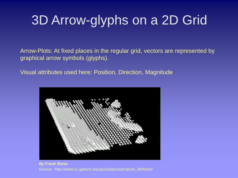
3D Arrow-glyphs on a 2D Grid

By Frank Reise Source : http://www.cc.gatech.edu/gvu/datavis/projects_98/frank/

Arrow-Plots: At fixed places in the regular grid, vectors are represented by graphical arrow symbols (glyphs). Visual attributes used here: Position, Direction, Magnitude

(C) Jean M. Favre, CSCS-Centro Svizzero di Calcolo Scientifico

http://www.siggraph.org/education/materials/HyperVis/vised/VisTech/Techniques/Examples/egv2dastreamparttracks.html

Streamlines Streamlines:

Seed points are released into the flow-field and advected with the flow. New particle positions are updated iteratively. The trace of a seed point is represented as a stream line. The vector field is assumed to be static. Interpolation in space.

Streamlines: Depicts structure of a flow field at fixed point in time Vector magnitude not immediately visible (i.e. distance between particle positions) Color coding of vector magnitude

Streaklines & Particle Tracing

Particle tracing: Particles are traced, but only current

position is subject to dynamic vector field.

Streaklines: Particles are moved depending on vector field.

Similar to particle tracking, but: Particle positions (also

previous) and vector field is updated at certain time leaps.

Visualizes the dynamics structure of a vector field over a certain time interval. For static vector fields, there is no difference compared with streamlines.

Streaklines & Particle Tracing

Streamlines: Gray dashed: Particle Traces: Red line Streaklines : Blue line

Source: Wikimedia Commons, Author: Fi1Kaiv8

Stream Ribbons The problem with streamlines and streaklines is that only the direction of flow of the field becomes evident. Rotations of the flow field around the flow axis and divergence and convergence of the field do not become visible. By connecting the traces of two adjacent streamlines, a ribbon band composed of polygons stretching between the two streamlines can be visualized. The orientation of the ribbon surface mediates rotational and contraction towards the direction of flow. The twist of the ribbon is an indicator for the streamwise vorticity of the field.

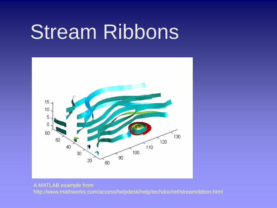
Stream Ribbons

A MATLAB example from http://www.mathworks.com/access/helpdesk/help/techdoc/ref/streamribbon.html

Stream Surfaces

• A extension or generalization of stream ribbons are stream surfaces.

• Stream surfaces are an infinite number of streamlines passing through a base curve or rake.

• In practice, a number of n seed points define the rake (user defined).

• N streamlines are bridged with polygons and form a more complex surface.

• Problems can occur with self-intersections and with separation (bifurcations).

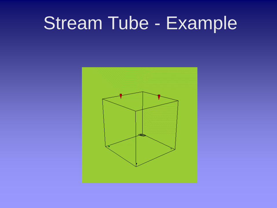
Stream Tube - Example

Stream Surfaces - Properties & Interpretation

• Stream surfaces reveal additional information on the structure of the vector field.

• Stream surfaces are tangential to the velocity vector • Hence, if e.g. vector field defines fluid flow, there is no transport of fluid through the stream surface • A circular rake will result in a s.k. stream tube

• Since there is no flux through the tube, the stream tube represents constant mass flux

Stream Polygons

• Used to reveal other local properties of vector fields/tensor fields

• If vector field describes flow of material this is due to local strain and rigid body motion.

• Strain (normal strain and shear strain), rotation -> deformation • Formally described as a strain matrix and rotation matrix i.e. 3x3 tensors

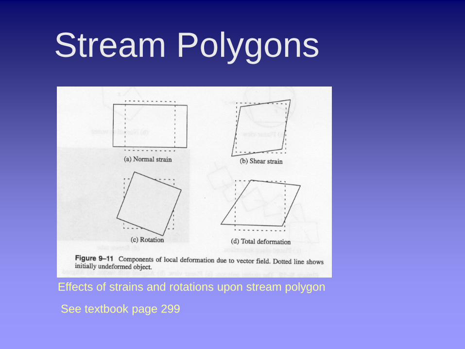
Stream Polygons

Effects of strains and rotations upon stream polygon

See textbook page 299

Stream Polygons

See textbook page 300

• Stream polygons are moved towards the direction of velocity vector.

• Polygon normal vector is aligned with velocity vector.

• Shear and normal strains deform the polygon.

• Rotation is about the polygon normal vector i.e. velocity vector.

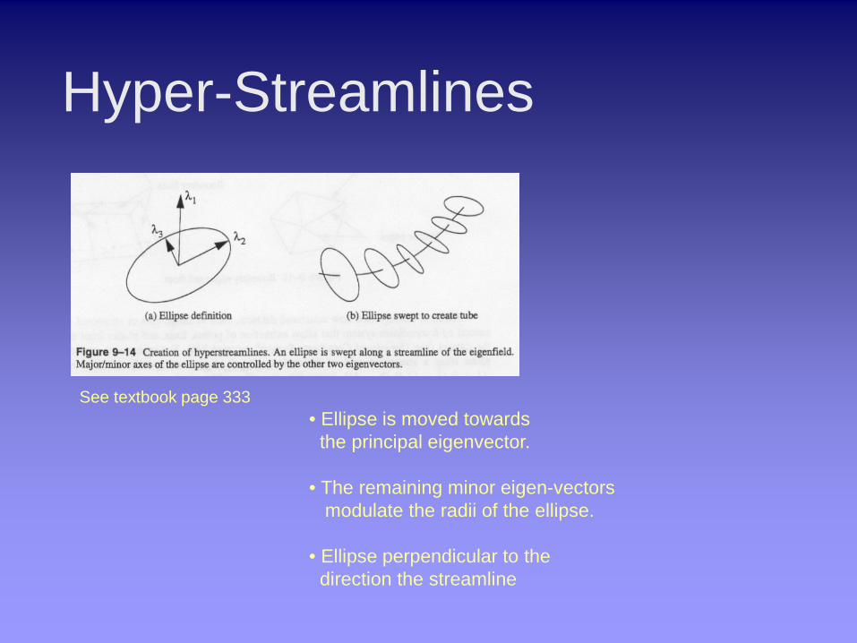
Hyper-Streamlines

See textbook page 333 • Ellipse is moved towards the principal eigenvector.

• The remaining minor eigen-vectors modulate the radii of the ellipse. • Ellipse perpendicular to the direction the streamline

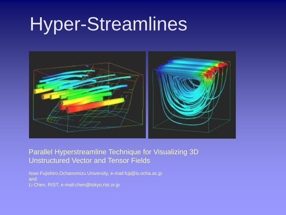
Hyper-Streamlines

Parallel Hyperstreamline Technique for Visualizing 3D Unstructured Vector and Tensor Fields

Issei Fujishiro,Ochanomizu University, e-mail:fuji@is.ocha.ac.jp and Li Chen, RIST, e-mail:chen@tokyo.rist.or.jp

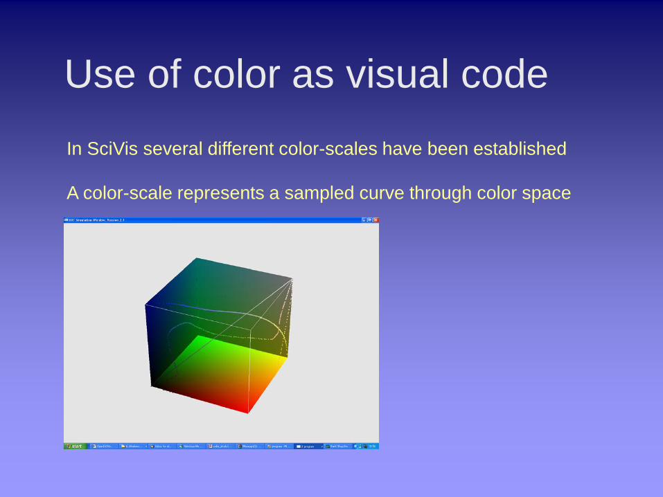
Use of color as visual code In SciVis several different color-scales have been established A color-scale represents a sampled curve through color space

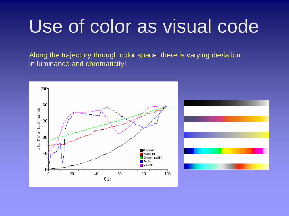
Use of color as visual code Along the trajectory through color space, there is varying deviation in luminance and chromaticity!

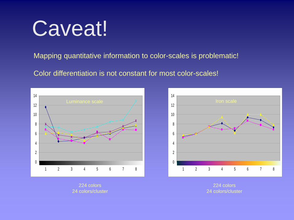
Caveat! Mapping quantitative information to color-scales is problematic! Color differentiation is not constant for most color-scales!

0

2

4

6

8

10

12

14

1 2 3 4 5 6 7 80

2

4

6

8

10

12

14

1 2 3 4 5 6 7 8

Luminance scale Iron scale

224 colors 24 colors/cluster

224 colors 24 colors/cluster

Visualization of time varying data in pulp process industry

The Lime Kiln – Part of the Recycling Process

Surveillance of temperatures Purpose: - Efficiency - Energy savings - Safety

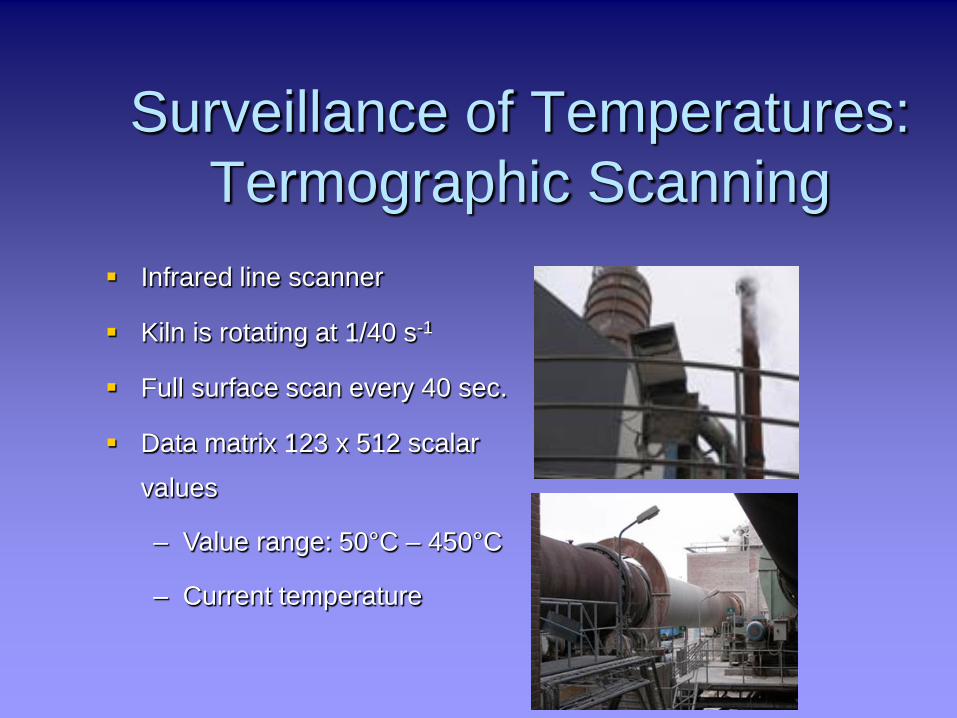
Surveillance of Temperatures: Termographic Scanning

Infrared line scanner

Kiln is rotating at 1/40 s-1

Full surface scan every 40 sec.

Data matrix 123 x 512 scalar

values

– Value range: 50°C – 450°C

– Current temperature

The operators’ task of visual investigation

Observe and visually analyze the graphical representation

Purpose : Detection of typical irregularities:

Bonded deposits -> slow dynamic process (days-weeks)

-> low variability of temperature

Variation in composition of fuel and chemicals -> relative slow process (hours to minutes)

-> relative low variability of temperature

Partial defects of insulation -> rapid dynamic process (minutes to seconds)

-> sudden increase of temperature

Assignment:

1. Discuss the visual task of the operators and classify the visualization problem according to the taxonomy of data in terms of attributes, domain, dimensions and nature of data!

2. Discuss general solutions in the InfoViz/SciViz that appear plausible to visualize the task-specific data.

3. Make a proposal for a visualization that would enhance the operators performance when identifying partial defects of insulation!

Use sketches and drawings to illustrate your design!

To be discussed on Thursday, 11th of October 2012 Get bonus on course grade if handed in in writing, max. 2 pages (A4) including sketches/figure. Include your name(s) and