Embed Size (px)
Citation preview
IMPROVEMENT OF THE PRIMARY LOW-FREQUENCY ACCELEROMETER CALIBRATION SYSTEM AT INMETRO
G.P. Ripper, C.D. Ferreira, R.S. Dias, G.B. Micheli, INMETRO / DIMCI / DIAVI /LAVIB
IMEKO 23rd TC3, 13th TC5 and 4th TC22 International Conference 30 May to 1 June, 2017, Helsinki, Finland

Outline of the presentation • Introduction • Description of the experiments
• New Calibration system
• Results and Discussions
• Conclusions

Introduction
• The Vibration Laboratory (Lavib) of INMETRO is continuously looking forward the improvement of its calibration systems and methods in order to fulfill the rising metrological demands in Brazil.
• Low-frequency vibration measurements are of interest in many different fields, as for instance: energy production, environmental assessment, transportation, etc.
Wind turbines Geophones Vibration analyzer for elevator

Low Frequency primary calibration system
1st Setup - Fringe Counting Method
Frequency range: 0.4 Hz to 160 Hz Exp. Unc. (k=2): 0.35 %
Diagram of the experimental setup (Fringe Counting Method)

Vibration exciter APS 129 Control accelerometer
Accelerometer under calibration
Electrodynamic vibration exciter
Linear guide Aluminum base
Aerostatic bearing
Modular mounting system
Mounting table
131,0
132,0
133,0
134,0
135,0
136,0
137,0
0,1 1 10 100 1000
Frequency [Hz]
Sens
itivi
ty [m
V/(m
/s2 )]
Su m1
Su m2
Su mean
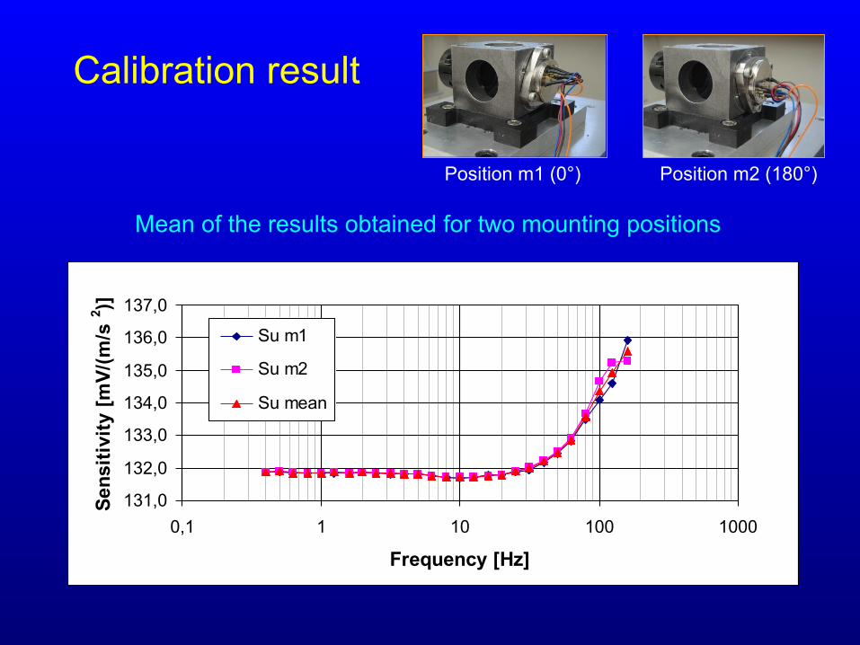
Calibration result
Mean of the results obtained for two mounting positions
Position m1 (0°) Position m2 (180°)
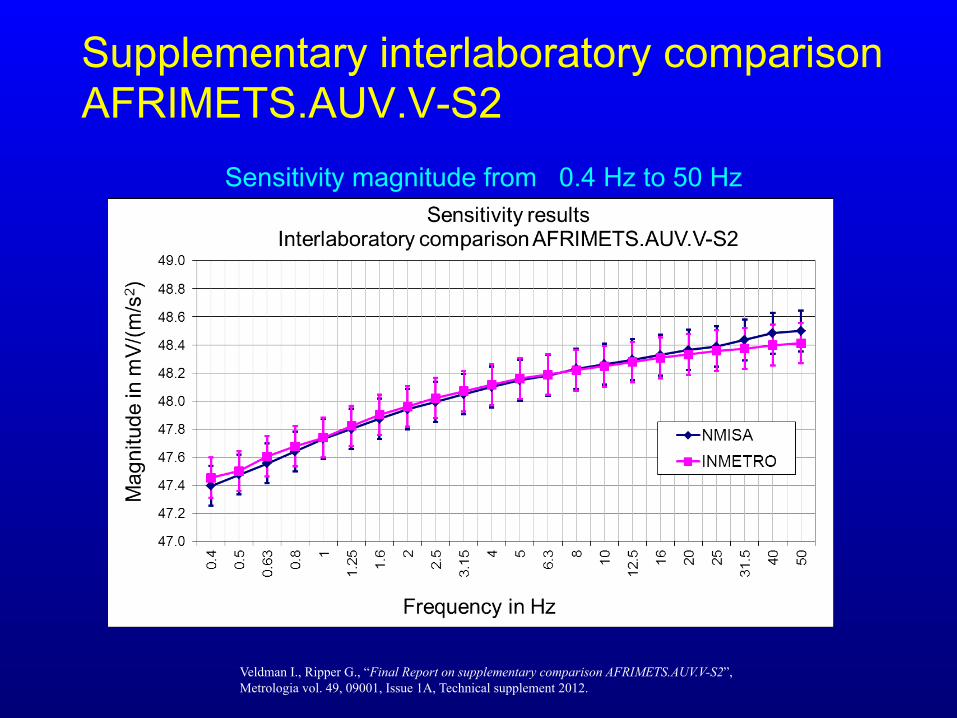
Supplementary interlaboratory comparison AFRIMETS.AUV.V-S2
Sensitivity magnitude from 0.4 Hz to 50 Hz
Veldman I., Ripper G., “Final Report on supplementary comparison AFRIMETS.AUV.V-S2”, Metrologia vol. 49, 09001, Issue 1A, Technical supplement 2012.
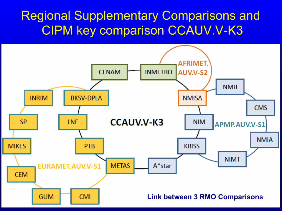
Regional Supplementary Comparisons and CIPM key comparison CCAUV.V-K3
Link between 3 RMO Comparisons
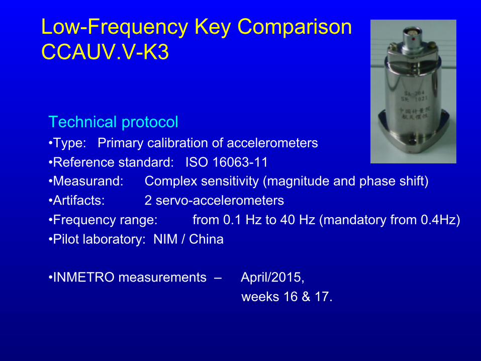
Low-Frequency Key Comparison CCAUV.V-K3
Technical protocol • Type: Primary calibration of accelerometers • Reference standard: ISO 16063-11 • Measurand: Complex sensitivity (magnitude and phase shift) • Artifacts: 2 servo-accelerometers • Frequency range: from 0.1 Hz to 40 Hz (mandatory from 0.4Hz) • Pilot laboratory: NIM / China
• INMETRO measurements – April/2015, weeks 16 & 17.
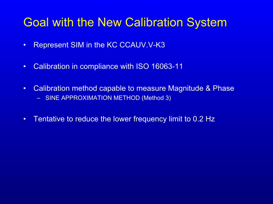
Goal with the New Calibration System
• Represent SIM in the KC CCAUV.V-K3
• Calibration in compliance with ISO 16063-11
• Calibration method capable to measure Magnitude & Phase – SINE APPROXIMATION METHOD (Method 3)
• Tentative to reduce the lower frequency limit to 0.2 Hz
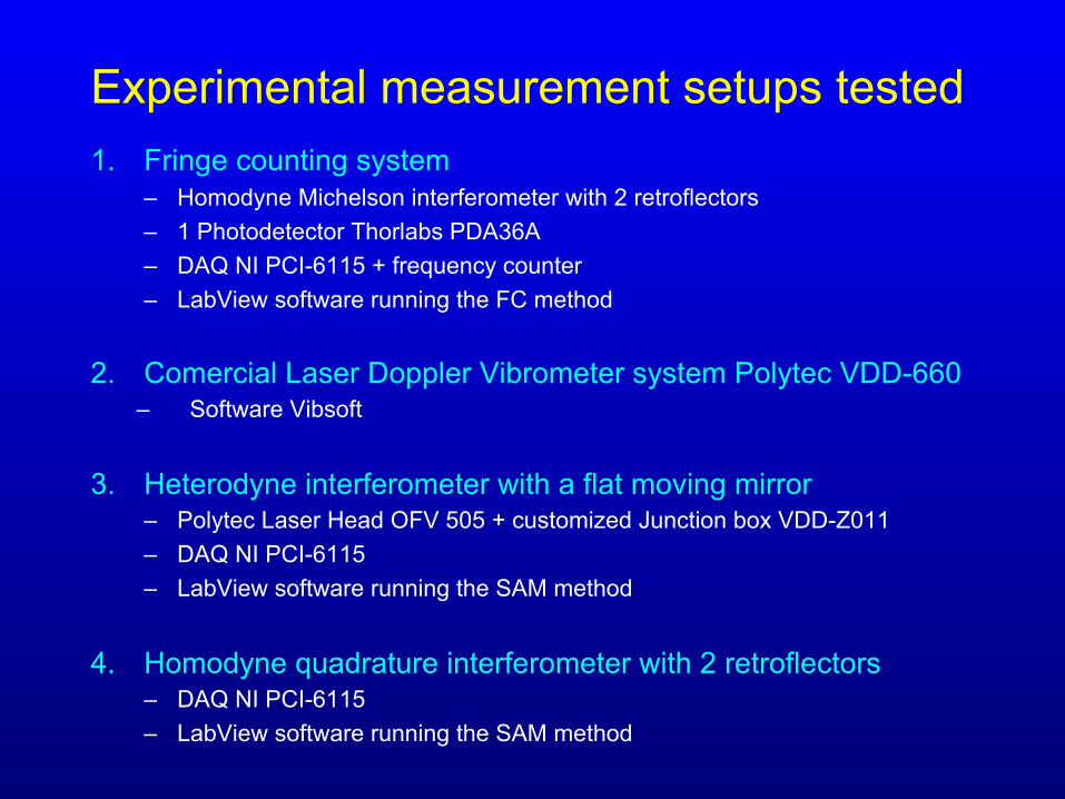
Experimental measurement setups tested 1. Fringe counting system
– Homodyne Michelson interferometer with 2 retroflectors – 1 Photodetector Thorlabs PDA36A – DAQ NI PCI-6115 + frequency counter – LabView software running the FC method
2. Comercial Laser Doppler Vibrometer system Polytec VDD-660 – Software Vibsoft
3. Heterodyne interferometer with a flat moving mirror – Polytec Laser Head OFV 505 + customized Junction box VDD-Z011 – DAQ NI PCI-6115 – LabView software running the SAM method
4. Homodyne quadrature interferometer with 2 retroflectors – DAQ NI PCI-6115 – LabView software running the SAM method

Computer
Comercial LDV Polytec VDD-660 + software Vibsoft 4.1
Junction Box VDD-Z011
Optical Head OFV-505
DAQ PCI NI-6110
Software VIBSOFT 4.1
accelerometer
I
Q
Vout
Polytec system
Signal Generator
f1
IEEE-488
Power Amplifier shaker
Manual setting of vibration level per frequency
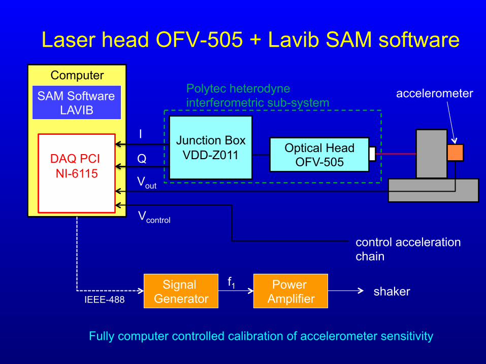
Computer
Laser head OFV-505 + Lavib SAM software
Junction Box VDD-Z011
Optical Head OFV-505
DAQ PCI NI-6115
SAM Software LAVIB
accelerometer
I
Q
Vout
Polytec heterodyne interferometric sub-system
control acceleration chain
Signal Generator
f1
IEEE-488
Power Amplifier shaker
Vcontrol
Fully computer controlled calibration of accelerometer sensitivity

Polytec laser vibrometer
VDD-660 system Modified junction box VDD-Z011 I & Q analog output signals A/D conversion with DAQ NI 6115 • 12 bit resolution • 4 channel simultaneous sampling • 10 MS/s max. sampling rate LabView software
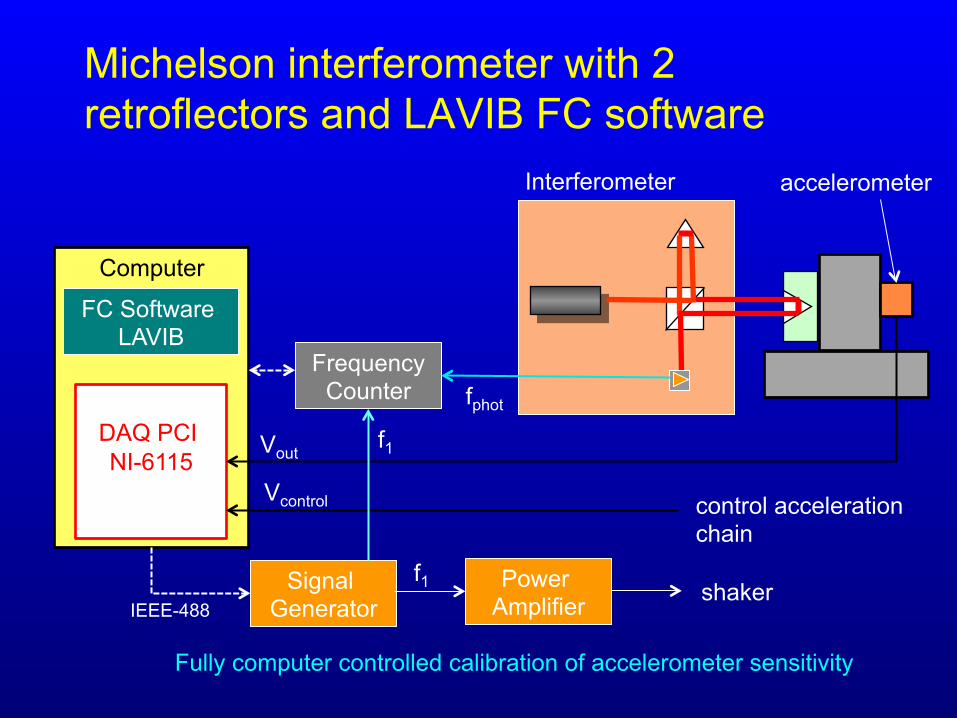
Computer
Michelson interferometer with 2 retroflectors and LAVIB FC software
DAQ PCI NI-6115
FC Software LAVIB
accelerometer
Vout
Interferometer
Frequency Counter
Signal Generator
f1
fphot
IEEE-488
f1 Power Amplifier shaker
control acceleration chain
Vcontrol
Fully computer controlled calibration of accelerometer sensitivity
Computer
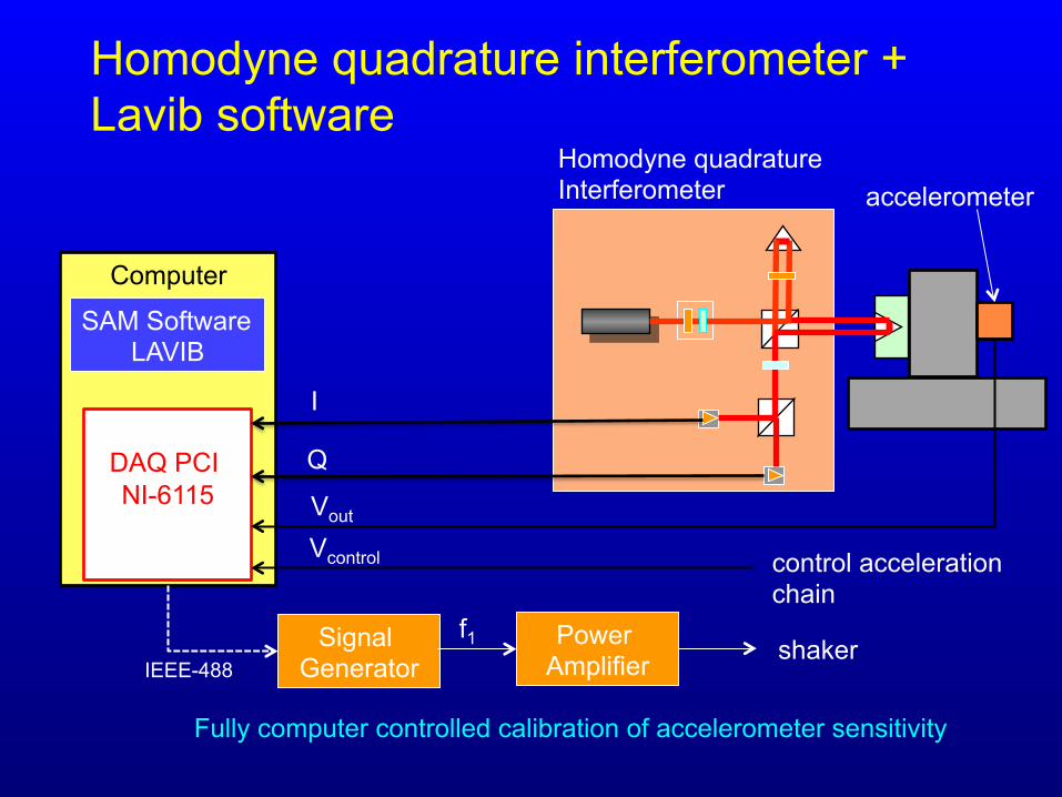
Homodyne quadrature interferometer + Lavib software
DAQ PCI NI-6115
SAM Software LAVIB
accelerometer
I
Q
Vout
Homodyne quadrature Interferometer
Signal Generator IEEE-488
f1 Power Amplifier shaker
control acceleration chain
Vcontrol
Fully computer controlled calibration of accelerometer sensitivity

Modified Michelson interferometer with two retroflectors
He-Ne Laser
Photodetector
Accelerometer Retroflector 2
Retroflector 1
s(t)
BS
u1(t)
Shaker table
intensidade luminosadeslocamento
Braços iguais no interferômetro (L=0)Interference
fringes
8ˆ λ
fRs =Displacement amplitude:
Fringes per vibra5on period: 1f
fR fotf =
)cos(ˆ)( 1 ststs ϕω +=

Homodyne quadrature interferometer with two retroflectors
He-Ne Laser
Photodetectors
PBS
Accelerometer Retroflector 2
Retroflector 1
)cos(ˆ)( 1tsts ω=
s(t)
P2
P1 WP-λ/4 BS
u1(t)
u2(t)
Opto-Isolator WP-λ/2
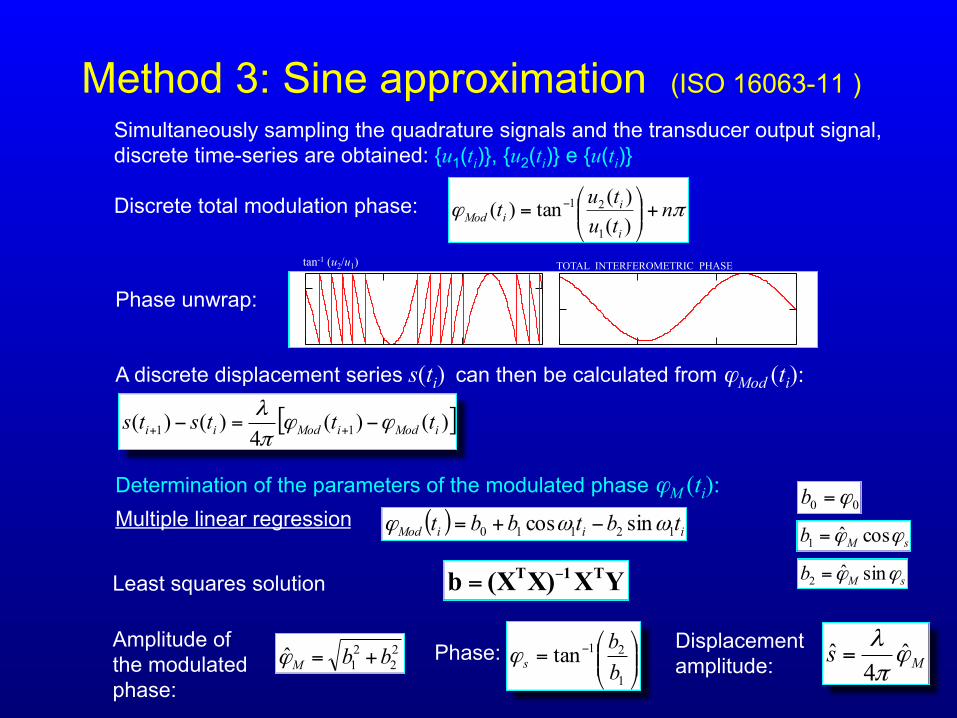
Method 3: Sine approximation (ISO 16063-11 ) Simultaneously sampling the quadrature signals and the transducer output signal, discrete time-series are obtained: {u1(ti)}, {u2(ti)} e {u(ti)}
Discrete total modulation phase: πϕ ntututi
iiMod +⎟⎟
⎠
⎞⎜⎜⎝
⎛= −
)()(tan)(
1
21
ARCTAN (u2/u1) FASE TOTAL DO SINAL INTERFEROMÉTRICO
Phase unwrap:
[ ])()(4
)()( 11 iModiModii tttsts ϕϕπλ
−=− ++
A discrete displacement series s(ti) can then be calculated from ϕMod (ti):
Determination of the parameters of the modulated phase ϕM (ti): Multiple linear regression ( ) iiiMod tbtbbt 12110 sincos ωωϕ −+=
YXX)(Xb T1T −=Least squares solution
22
21ˆ bbM +=ϕ ⎟⎟
⎠
⎞⎜⎜⎝
⎛= −
1
21tanbb
sϕAmplitude of the modulated phase:
Phase: Displacement amplitude: Ms ϕ
πλ ˆ4
ˆ =
sMb ϕϕ cosˆ1 =
sMb ϕϕ sinˆ2 =
00 ϕ=b
TOTAL INTERFEROMETRIC PHASE tan-1 (u2/u1)

Method 3: Sine approximation
Multiple linear regression
YXX)(Xb T1T −=Least squares solution:
Signal amplitude: Phase:
iuiui tututu 11 sinsinˆcoscosˆ)( ωϕωϕ −=
iuiuui tbtbbtu 12110 sincos)( ωω −+=
The equation for the transducer output can be written in its discrete form:
uu ub ϕcosˆ1 =
uu ub ϕsinˆ2 =
constant0 =ub
22
21ˆ uu bbu += ⎟⎟
⎠
⎞⎜⎜⎝
⎛= −
1
21tanu
uu b
bϕ
auSua ˆˆˆ = ( )au ϕϕϕ −=Δ
Mfa ϕπλ ˆˆ 2= πϕϕ += sa
Sensitivity:
Amplitude: Phase shift:
Acceleration amplitude: Phase:
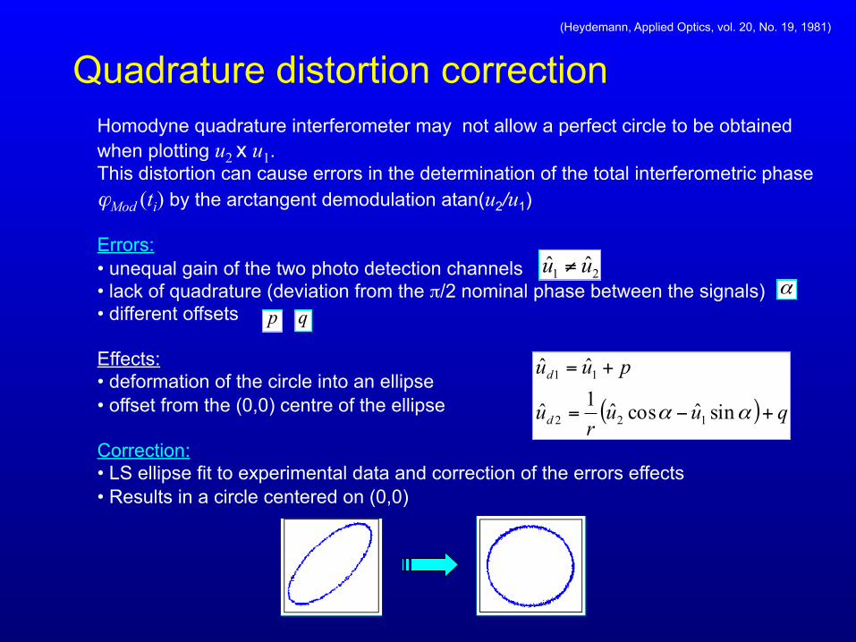
Quadrature distortion correction Homodyne quadrature interferometer may not allow a perfect circle to be obtained when plotting u2 x u1. This distortion can cause errors in the determination of the total interferometric phase ϕMod (ti) by the arctangent demodulation atan(u2/u1) Errors: • unequal gain of the two photo detection channels • lack of quadrature (deviation from the π/2 nominal phase between the signals) • different offsets
Effects: • deformation of the circle into an ellipse • offset from the (0,0) centre of the ellipse Correction: • LS ellipse fit to experimental data and correction of the errors effects • Results in a circle centered on (0,0)
21 ˆˆ uu ≠
( ) quur
u
puu
d
d
+−=
+=
αα sinˆcosˆ1ˆ
ˆˆ
122
11
(Heydemann, Applied Optics, vol. 20, No. 19, 1981)
αp q

Homodyne quadrature interferometer
R2 R1
PBS
WP- λ/2 WP-λ/4
P Laser
Ph2 Ph1
BS
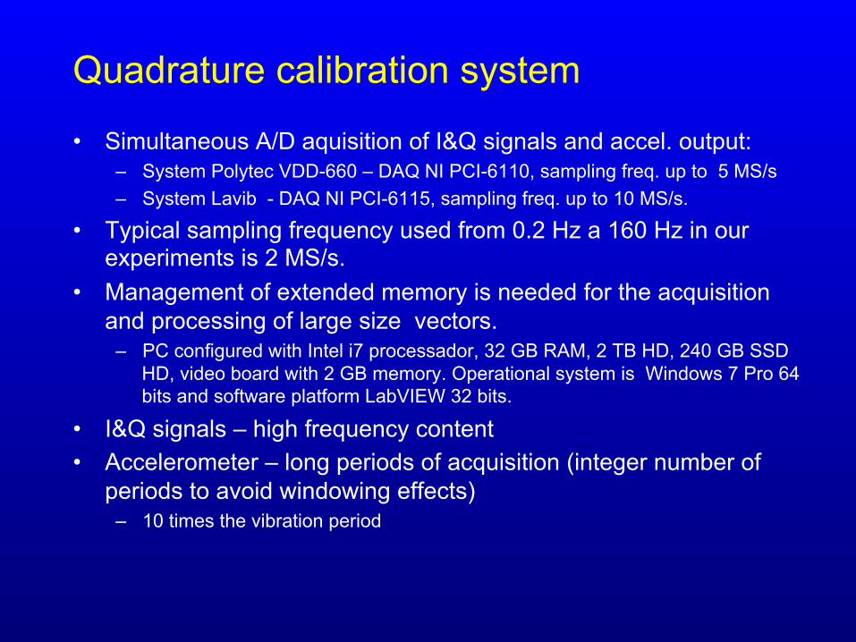
Quadrature calibration system
• Simultaneous A/D aquisition of I&Q signals and accel. output: – System Polytec VDD-660 – DAQ NI PCI-6110, sampling freq. up to 5 MS/s – System Lavib - DAQ NI PCI-6115, sampling freq. up to 10 MS/s.
• Typical sampling frequency used from 0.2 Hz a 160 Hz in our experiments is 2 MS/s.
• Management of extended memory is needed for the acquisition and processing of large size vectors.
– PC configured with Intel i7 processador, 32 GB RAM, 2 TB HD, 240 GB SSD HD, video board with 2 GB memory. Operational system is Windows 7 Pro 64 bits and software platform LabVIEW 32 bits.
• I&Q signals – high frequency content • Accelerometer – long periods of acquisition (integer number of
periods to avoid windowing effects) – 10 times the vibration period

Lavib SAM software - Streaming to disk
• Software was developed to optimize the use of PC memory
• Packages of data with fixed length are A/D converted and streamed to disc in a cyclic process.
• These packages are later recovered and appended in sequence to obtain data vectors with the resolution and length compatible with each vibration frequency.
• After applying the arctangent demodulation and phase unwrap algorithm data decimation is used to reduce vectors size
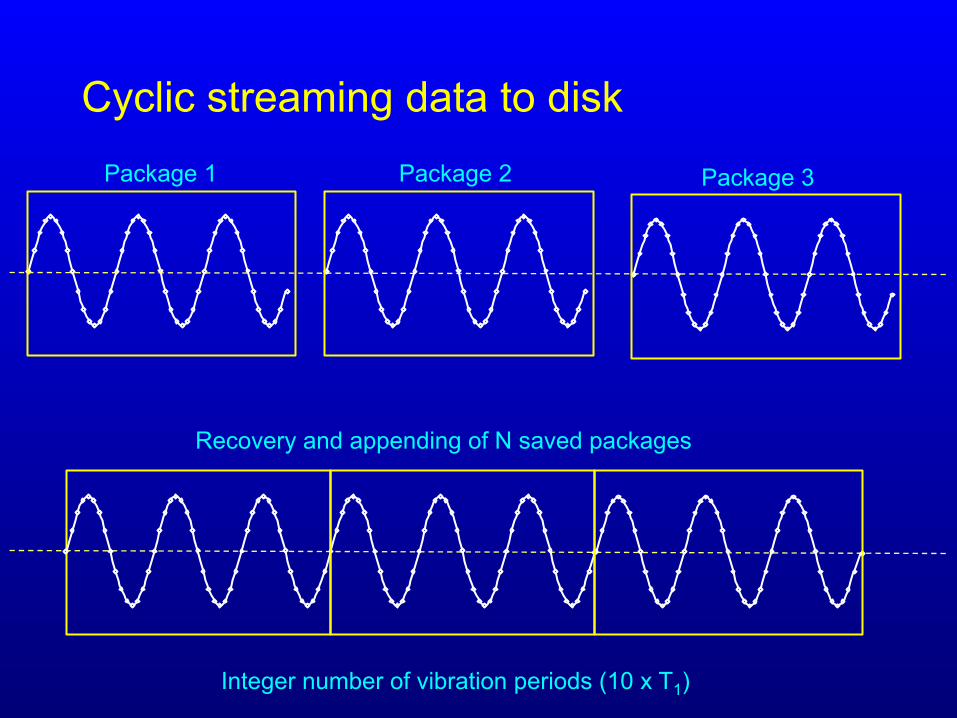
Cyclic streaming data to disk Package 1
Recovery and appending of N saved packages
Package 2 Package 3
Integer number of vibration periods (10 x T1)

Acquisition parameters Frequency
[Hz[ Period
[s] # Samples
Sampling rate [Samples/s]
# packages
Acquisition time [s]
# Cycles
0.2 5 250000 2000000 400 50 10 0.25 4 250000 2000000 320 40 10
0.315 3.17460317 125000 2000000 3200 200 63 0.4 2.5 500000 2000000 100 25 10 0.5 2 500000 2000000 80 20 10
0.63 1.58730158 125000 2000000 1600 100 63 0.8 1.25 250000 2000000 100 12.5 10 1 1 250000 2000000 80 10 10
1.25 0.8 250000 2000000 64 8 10 1.6 0.625 250000 2000000 50 6.25 10 2 0.5 250000 2000000 40 5 10
2.5 0.4 250000 2000000 32 4 10 3.15 0.31746031 250000 2000000 160 20 63
4 0.25 250000 2000000 20 2.5 10 5 0.2 250000 2000000 16 2 10
6.3 0.15873015 250000 2000000 80 10 63 8 0.125 250000 2000000 10 1.25 10
10 0.1 2000000 2000000 1 1 10 12.5 0.08 2000000 2000000 2 2 25 16 0.0625 2000000 2000000 1 1 16 20 0.05 2000000 2000000 1 1 20 25 0.04 2000000 2000000 1 1 25
31.5 0.03174603 2000000 2000000 2 2 63 40 0.025 2000000 2000000 1 1 40 50 0.02 2000000 2000000 1 1 50

Data processing (example for 1 Hz)
SAMs
sSAMϕs (ti)
Recovery of I&Q signals
saved to disk (T = 0.125 s)
2 MSa/s 250 kSa
Ellipse fit
Correction
Phase unwrap
πλ4
×
⎟⎟⎠
⎞⎜⎜⎝
⎛−
1
21tanc
c
uu
Decimation (factor = 20)
Save reduced data to disk
(T = 10 s) 12.5 kSa
SAM
I (t)
Q(t)
A/D conversion
Rate = 2 MSa/s # Samples =250 kSa
Save package
to disk (T = 0,125 s)
2 Stacks of 80
packages (T = 10 s)
Length = 20 MSa
Repeat for N packages
Interferometric signals
Repeat for N packages
1 Stack of 80
reduced packages (T = 10 s)
Length = 1 MSa
displacement vector

Data processing (example for 1 Hz)
SAMû
uSAMϕu (ti)
Recovery of I&Q signals
saved to disk (T = 0.125 s)
2 MSa/s 250 kSa
Decimation (factor = 20)
Save reduced data to disk
(T = 10 s) 12.5 kSa
SAM
u (t)
A/D conversion Rate = 2 MSa/s
# Samples =250 kSa
Save package
to disk (T = 0,125 s)
2 Stacks of 80
packages (T = 10 s)
Length = 20 MSa
Repeat for N packages
Transducer output signal
Repeat for N packages
1 Stack of 80
reduced packages (T = 10 s)
Length = 1 MSa
Transducer output vector
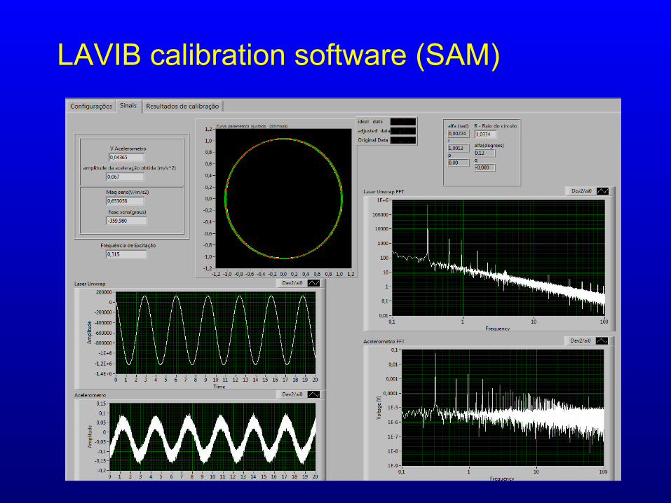
LAVIB calibration software (SAM)

Calibration results Servo-accelerometer Allied Signal QA-3000 + 5 kΩ shunt resistor
A deviation can be observed above 5 Hz, when the acceleration level rises from 2 m/s2 up to 3,5 m/s2. This increase in acceleration level is usually applied to improve the signal-to-noise ratio on the transducer output signal
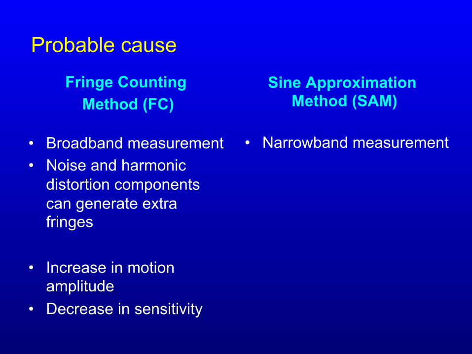
Probable cause
Fringe Counting Method (FC)
• Broadband measurement • Noise and harmonic
distortion components can generate extra fringes
• Increase in motion amplitude
• Decrease in sensitivity
Sine Approximation Method (SAM)
• Narrowband measurement
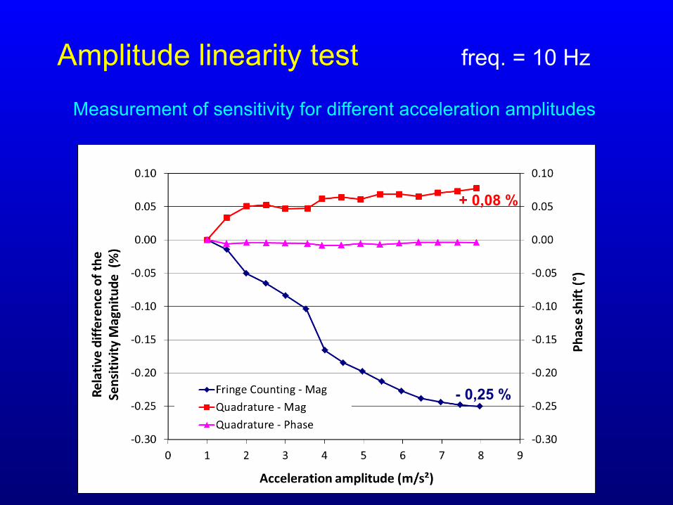
Amplitude linearity test freq. = 10 Hz
Measurement of sensitivity for different acceleration amplitudes
+ 0,08 %
- 0,25 %

Amplitude linearity test freq. = 10 Hz
Measurement of sensitivity for different acceleration amplitudes

Phase response Comparison of results from 3 measurement setups
SAM Difference smaller than 0,01º
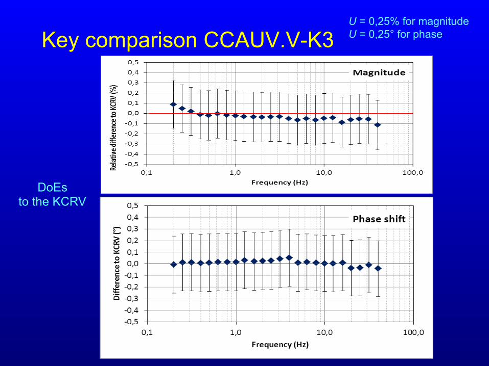
Key comparison CCAUV.V-K3
DoEs to the KCRV
U = 0,25% for magnitude U = 0,25° for phase
Conclusions • The new system presented allowed INMETRO to improve its
measurement capability for vibration calibrations in low frequencies.
• SAM presents higher immunity to noise and THD than FC
• Primary calibrations of complex sensitivity (mag & phase) are already possible from 0.2 Hz to 160 Hz.
• Current CMC of INMETRO for magnitude - Exp. Unc. is 0.35%
• Key comparison CCAUV.V-K3 allowed us to check the equivalence between results obtained by several NMIs – Lower uncertainty was reported using the new system : 0.25% for magnitude and 0.25o for phase – Calculated DoEs smaller than 0.15% for magnitude and 0.1o for phase