Improving Autonomous Performance of a Passive Morphing

Information Technology and Control 2020/1/4928

Improving Autonomous Performance of a Passive Morphing Fixed Wing UAV

ITC 1/49Information Technology and ControlVol. 49 / No. 1 / 2020pp. 28-35DOI /10.5755/j01.itc.49.1.23275

Improving Autonomous Performance of a Passive Morphing Fixed Wing UAV

Received 2019/05/19 Accepted after revision 2019/12/17

http://dx.doi.org//10.5755/j01.itc.49.1.23275

HOW TO CITE: Coban, S., Bilgic, H. H., & Akan, E. (2020). Improving Autonomous Performance of a Passive Morphing Fixed Wing UAV. Information Technology and Control, 49(1), 28-35. https://doi.org//10.5755/j01.itc.49.1.23275

Corresponding author: [email protected]

Sezer CobanFaculty of Aeronautics and Astronautics; Iskenderun Technical University; Iskenderun, Turkey; phone: +90 326 613 56 00 (Ext: 5213); e-mail: [email protected]

Hasan Huseyin BilgicFaculty of Engineering and Natural Sciences; Iskenderun Technical University; Iskenderun, Turkey; phone: +90 326 613 56 00 (Ext: 2419); e-mail: [email protected]

Ercan AkanBarbaros Hayrettin Faculty of Naval Architecture and Maritime; Iskenderun Technical University; Iskenderun, Turkey; phone: +90 326 613 56 00 (Ext: 3020); e-mail: [email protected]

In this article, simultaneous longitudinal and lateral flight control systems design for both passive and active mor-phing unmanned aerial vehicles (UAVs) is first time applied for autonomous flight performance maximization. For this purpose, an UAV whose wing and tail unit can be assembled to fuselage from different points in a pre-scribed interval and whose wing and tail can move forward and backward independently in tail to nose direction is manufactured. Following this, an autopilot is purchased and it lets change of P, I, D coefficients in certain intervals. First, dynamic model and longitudinal and lateral state space models of UAV are obtained and then simulation model is reached. At the same time, block diagram of autopilot system and modeling of it in MATLAB/Simulink environment are found. After these, using these two models and adaptive stochastic optimization method, name-ly, SPSA, simultaneous design of UAV and autopilot is applied in order to minimize a cost function consisting of rise time, settling time and maximum overshoot. Therefore, primarily autonomous performance is maximized in computer environment. Moreover, high performance is observed at simulation responses.KEYWORDS: UAV (Unmanned Aerial Vehicle), Dynamic Model, State Space Model, PID, Simulink.

mailto:[email protected]

29Information Technology and Control 2020/1/49

1. Introduction Studies on the morphing of UAV have been increas-ing in recent years. The motivation behind morphing has been to find new ways to boost the capabilities of aircraft. This paper concentrates on UAV morphing concepts, designs and control technologies. Aircraft wings are a structural part that allows the aircraft to fly in various flight conditions, but their performance can be improved. The ability to change the geometry of the wing surface before and during the flight attracts researchers and designers. Morph-ing means a change of shape, but there is no accept-ed definition in aviation. Changing the wing shape or geometry is not a new working area. In the literature, morphing solutions always have disadvantages in terms of cost, complexity or weight, but in some cases provide several benefits to the system. Recent devel-opments in smart materials can overcome limitations and increase benefits from existing design solutions. The challenge is to design a structure that can with-stand the prescribed loads, but can also change the shape of the structure. Ideally, there should be no distinction between the wing and the fuselage. Mor-phing is a promising technology for a new generation aircraft. However, manufacturers and end users still doubt about the benefits of adopting morphing in the near future. This paper provides a review of the latest technology in morphing aircraft and focuses on struc-tural, deforming morphing concepts for fixed wings, particularly with reference to active systems. Re-searchers have carried out many studies on the mod-eling and control of unmanned aerial vehicles [8-15].An Unmanned Aerial Vehicle (UAV) can move freely in three imaginary axes that intersect and are per-pendicular to the center of gravity. To be able to say that this aircraft has been fully inspected, the pilot or automatic control systems must have control over the movement of these three imaginary axes. The Vertical Axis is that extending from the upper body through the center of gravity of the aircraft. Movement around this axis is called yaw motion. Yaw moves the nose of the aircraft to the right or left relative to the vertical axis. The longitudinal axis is the axis that extends from the nose to the tail of the aircraft, which crosses the aircraft and passes through the center of gravity. Motion around this axis is called ’roll’. The motion of the aircraft around this axis is controlled by flap,

elevator or spoiler. The lateral axis is the axis that crosses the aircraft from one wing end to the other wing end and then passes through the center of gravi-ty. Movement around this axis is called pitch motion. Pitch occurs when the aircraft changes its angle of attack, meaning that it moves to climb or dive [12]. The pitch movement of the aircraft around this axis is controlled by the elevators, movable horizontal stabi-lizers and elevators.

2. UAV Designing and ManufacturingThe design of UAV was completed on computer en-vironment by using Solidworks program. A detailed drawing of all parts of the UAV during design was made. The top view of our unmanned aerial vehicle is given in Figure 1 [2].

Figure 1 Top view of UAV

1. Introduction Studies on the morphing of UAV have been increasing in recent years. The motivation behind morphing has been to find new ways to boost the capabilities of aircraft. This paper concentrates on UAV morphing concepts, designs and control technologies.

Aircraft wings are a structural part that allows the aircraft to fly in various flight conditions, but their performance can be improved. The ability to change the geometry of the wing surface before and during the flight attracts researchers and designers. Morphing means a change of shape, but there is no accepted definition in aviation. Changing the wing shape or geometry is not a new working area. In the literature, morphing solutions always have disadvantages in terms of cost, complexity or weight, but in some cases provide several benefits to the system. Recent developments in smart materials can overcome limitations and increase benefits from existing design solutions. The challenge is to design a structure that can withstand the prescribed loads, but can also change the shape of the structure. Ideally, there should be no distinction between the wing and the fuselage. Morphing is a promising technology for a new generation aircraft. However, manufacturers and end users still doubt about the benefits of adopting morphing in the near future. This paper provides a review of the latest technology in morphing aircraft and focuses on structural, deforming morphing concepts for fixed wings, particularly with reference to active systems. Researchers have carried out many studies on the modeling and control of unmanned aerial vehicles [8-15].

An Unmanned Aerial Vehicle (UAV) can move freely in three imaginary axes that intersect and are perpendicular to the center of gravity. To be able to say that this aircraft has been fully inspected, the pilot or automatic control systems must have control over the movement of these three imaginary axes. The Vertical Axis is that extending from the upper body through the center of gravity of the aircraft. Movement around this axis is called yaw motion. Yaw moves the nose of the aircraft to the right or left relative to the vertical axis. The longitudinal axis is the axis that extends from the nose to the tail of the aircraft, which crosses the aircraft and passes through the center of gravity. Motion around this axis is called ’roll’. The motion of the aircraft around this axis is controlled by flap, elevator or spoiler. The lateral

axis is the axis that crosses the aircraft from one wing end to the other wing end and then passes through the center of gravity. Movement around this axis is called pitch motion. Pitch occurs when the aircraft changes its angle of attack, meaning that it moves to climb or dive [12]. The pitch movement of the aircraft around this axis is controlled by the elevators, movable horizontal stabilizers and elevators.

2. UAV Designing and

Manufacturing The design of UAV was completed on computer environment by using Solidworks program. A detailed drawing of all parts of the UAV during design was made. The top view of our unmanned aerial vehicle is given in Figure 1 [2].

FFiigguurree 11

Top view of UAV

As a result of the designing, the parts of the body components were cut from the depron and the plywood in the laser cutting device. Body parts are glued together with epoxy adhesive. Wing and tail profile is produced using CNC cutting device. For the wing and tail set, the necessary reinforcements were made by using balsa, plywood and carbon rod. Aileron, elevator and rudder were produced. All outer surfaces were covered

As a result of the designing, the parts of the body com-ponents were cut from the depron and the plywood in the laser cutting device. Body parts are glued together


with epoxy adhesive. Wing and tail profile is produced using CNC cutting device. For the wing and tail set, the necessary reinforcements were made by using balsa, plywood and carbon rod. Aileron, elevator and rudder were produced. All outer surfaces were cov-ered with coating. Transformation mechanism for wing and tail set was produced. Aileron, elevator and rudder were assembled. Front and rear landing gear were produced and assembled [4]. In Figure 2, UAV body and wing skeleton view and in Figure 3, the final version of the UAV are presented.

Figure 3The final version of the UAV

with coating. Transformation mechanism for wing and tail set was produced. Aileron, elevator and rudder were assembled. Front and rear landing gear were produced and assembled [4]. In Figure 2, UAV body and wing skeleton view and in Figure 3, the final version of the UAV are presented. FFiigguurree 22 UAV body and wing skeleton view

FFiigguurree 33

The final version of the UAV

3. UAV Dynamic Modeling In order to perform any dynamic modeling of any aeronautical vehicle or any UAV, it is necessary to obtain the governing equations of the aircraft body. These equations can be classified into three groups. These equations are the equations of force, moment equations and kinematic equations of the body. Newton's second law was used in the literature to extract the force equations [11]:

.cg

II I A

cg cga a= = +

dV VF M M ω V

dt t⊗

∂ ∂

(1)

The components of the force on the three axes (X, Y, Z) can be expressed in terms of the weight of the aircraft, linear accelerations, linear velocities

(u, v, w), angular velocities (p, q, r) and Euler orientation angles as follows [9]:

( ) sin( )( ) cos( )sin( ) .( ) cos( )sin( )

a a A

a aA A A

a a A A

X M u qw rv M gF Y M v ru pw M g

Z M w pv qu M g

θθ φθ φ

+ − +

= = + − −

+ − −

(2)

In order to extract the moment equations, the law of conservation of angular momentum, which is widely used in the literature, has been used. In Equation (3), this law is granted [14]:

I I A II = + h h ω ht ⊗

∂∂

. (3)

In Figure 4, the linear and angular velocity components in an aircraft (in the aircraft axis assembly) are presented visually. In Figure 5, the relationships between the speed components and the off-shore and side-strap angles are presented in an aircraft.

FFiigguurree 44

Linear and angular velocity components for aircraft (airborne axis team)

FFiigguurree 55

Ramp and side strap angles with speed components in an air tool


FFiigguurree 33



.cg

II I A

cg cga a= = +

dV VF M M ω V

dt t⊗

∂ ∂

(1)




a a A

a aA A A

a a A A


Z M w pv qu M g

θθ φθ φ

+ − +

= = + − −

+ − −

(2)



∂∂

. (3)


FFiigguurree 44


FFiigguurree 55


Figure 2 UAV body and wing skeleton view

3. UAV Dynamic ModelingIn order to perform any dynamic modeling of any aeronautical vehicle or any UAV, it is necessary to obtain the governing equations of the aircraft body. These equations can be classified into three groups. These equations are the equations of force, moment

equations and kinematic equations of the body. New-ton’s second law was used in the literature to extract the force equations [11]:


FFiigguurree 33



.cg

II I A

cg cga a= = +

dV VF M M ω V

dt t⊗

∂ ∂

(1)




a a A

a aA A A

a a A A


Z M w pv qu M g

θθ φθ φ

+ − +

= = + − −

+ − −

(2)



∂∂

. (3)


FFiigguurree 44


FFiigguurree 55


(1)

The components of the force on the three axes (X, Y, Z) can be expressed in terms of the weight of the air-craft, linear accelerations, linear velocities (u, v, w), angular velocities (p, q, r) and Euler orientation an-gles as follows [9]:


FFiigguurree 33



.cg

II I A

cg cga a= = +

dV VF M M ω V

dt t⊗

∂ ∂

(1)




a a A

a aA A A

a a A A


Z M w pv qu M g

θθ φθ φ

+ − +

= = + − −

+ − −

(2)



∂∂

. (3)


FFiigguurree 44


FFiigguurree 55


(2)



FFiigguurree 33



.cg

II I A

cg cga a= = +

dV VF M M ω V

dt t⊗

∂ ∂

(1)




a a A

a aA A A

a a A A


Z M w pv qu M g

θθ φθ φ

+ − +

= = + − −

+ − −

(2)



∂∂

. (3)


FFiigguurree 44


FFiigguurree 55


(3)

In Figure 4, the linear and angular velocity compo-nents in an aircraft (in the aircraft axis assembly) are presented visually. In Figure 5, the relationships between the speed components and the off-shore and side-strap angles are presented in an aircraft.

Figure 4Linear and angular velocity components for aircraft (airborne axis team)


FFiigguurree 33



.cg

II I A

cg cga a= = +

dV VF M M ω V

dt t⊗

∂ ∂

(1)




a a A

a aA A A

a a A A


Z M w pv qu M g

θθ φθ φ

+ − +

= = + − −

+ − −

(2)



∂∂

. (3)


FFiigguurree 44


FFiigguurree 55



3. State-Space ModelStability derivatives are obtained by using stability derivative coefficients. The state space model is de-rived using these obtained stability derivatives. Nu-merical values are obtained by using the geometric data of the unmanned aerial vehicle. Longitudinal state space model of UAV is given in Equation (4):

δ δ

δ δ

δ δ δ δ

θ θ

δ

δ

−∆ ∆∆ ∆

=+ + +∆ ∆

∆ ∆

∆+

+ + ∆

0

0

.

000

0 0 1 0

0 0

u w

u w

u w w w w w q w

eT

TeT

w w ee eT T

X X gu uZ Z uw w

M M Z M M Z M M uq q

X X

Z Z

M M Z M M Z

L(4)

Lateral state space model is given in Equation (5) [16]:

4. State-Space Model Stability derivatives are obtained by using stability derivative coefficients. The state space model is derived using these obtained stability derivatives. Numerical values are obtained by using the geometric data of the unmanned aerial vehicle. Longitudinal state space model of UAV is given in Equation (4):

( )δ δ

δ δ

δ δ δ δ

θ θ

δ

δ

−∆ ∆∆ ∆

=+ + +∆ ∆

∆ ∆

∆+

+ + ∆

0

0

.

000

0 0 1 0

0 0

4

u w

u w

u w w w w w q w

eT

TeT

w w ee eT T

X X gu uZ Z uw w

M M Z M M Z M M uq q

X X

Z Z

M M Z M M Z

L

ateral state space model is given in Equation (5) [16]:

δ

δ δ δ δ

δ

θ

φ φ

− − −

∆ ∆+ + +

∆ ∆=

∆ ∆+ + +∆ ∆

+ +

+

+

0 0

* * * * * *

* * * * * *

* * *

*

( ) cos( )

0

0

0 1 0 0

0

*

v p r

xz xzw v p p r r

x x

xz xz xzv v p p r r

z z z

r

xz xza a r r

x x

a

Y Y u Y g

I I Iv vxzL N L N L Np pI I Ixr rI I I

N L N L N LI I I

Y

I IL N L N

I I

N δ δ δ

δ

δ

∆

∆+

* .

* *

0 0

a

xz xz ra r r

z z

I IL N L

I I

By examining the eigenvalues of state-space models obtained as a result of dynamic modeling, it can be decided that the models we create are correct. Figures 6 and 7 show the longitudinal and lateral flight modes, respectively. Therefore, it can be claimed that our dynamic modeling process is correct [6].

FFiigguurree 66 Longitudinal motion modes of UAV

FFiigguurree 77 Lateral motion modes of UAV

5. Wing and Structural

Analysis of UAV Figure 8 shows the aerodynamic coefficient values of UAV at different attack angles, such as 0 °, 4 ° and 8 °.

FFiigguurree 88 Aerodynamic coefficients at (a) 0 ° attack angle, (b) 4 ° attack angle, (c) 8 ° attack angle (a)

(b)

(c)

(5)

Figure 5Ramp and side strap angles with speed components in an air tool


FFiigguurree 33



.cg

II I A

cg cga a= = +

dV VF M M ω V

dt t⊗

∂ ∂

(1)




a a A

a aA A A

a a A A


Z M w pv qu M g

θθ φθ φ

+ − +

= = + − −

+ − −

(2)



∂∂

. (3)


FFiigguurree 44


FFiigguurree 55


By examining the eigenvalues of state-space models obtained as a result of dynamic modeling, it can be de-cided that the models we create are correct. Figures 6 and 7 show the longitudinal and lateral flight modes, respectively. Therefore, it can be claimed that our dy-namic modeling process is correct [6].

Figure 6Longitudinal motion modes of UAV

Figure 7Lateral motion modes of UAV

5. Wing and Structural Analysis of UAVFigure 8 shows the aerodynamic coefficient values of UAV at different attack angles, such as 0 °, 4 ° and 8 °.When we increase the wing profile at angles of 0° to 20° in angles of attack, the aerodynamic coefficients will change for each angle of attack. According to the results of the analysis, it is observed that the wing profile is stalled after 16° of attack (Figure 9).Figure 10(a) shows the deviation of the UAV on the wing. The deviation is increased as the wing moves to-wards the tip and reaches the highest value when the end of the wing is reached. Figure 10(b) shows the Von


Figure 8 Aerodynamic coefficients at (a) 0 ° attack angle, (b) 4 ° attack angle, (c) 8 ° attack angle

Figure 9 Angle of attack when entering the stall profile

(a)

(b)

(c)

Mises stress values on the wing of the UAV. Von Mises stress values vary according to the change in bending resistance. As a result, the largest Von Mises strain val-ue is found at the root of the wing. The best place for carbon tubes is where the voltage produced by the foam and carbon tubes is below the maximum voltage value.

Figure 10 Von mises stress results (80 km /h)

5. Wing and Structural

Analysis of UAV Figure 8 shows the aerodynamic coefficient values of UAV at different attack angles, such as 0 °, 4 ° and 8 °.

Figure 8 Aerodynamic coefficients at (a) 0 ° attack angle, (b) 4 ° attack angle, (c) 8 ° attack angle (a)

(b)

(c)

Figure 9 Angle of attack when entering the stall profile

When we increase the wing profile at angles of 0° to 20° in angles of attack, the aerodynamic coefficients will change for each angle of attack. According to the results of the analysis, it is observed that the wing profile is stalled after 16° of attack (Figure 9). Figure 10(a) shows the deviation of the UAV on the wing. The deviation is increased as the wing moves towards the tip and reaches the highest value when the end of the wing is reached. Figure 10(b) shows the Von Mises stress values on the wing of the UAV. Von Mises stress values vary according to the change in bending resistance. As a result, the largest Von Mises strain value is found at the root of the wing. The best place for carbon tubes is where the voltage produced by the foam and carbon tubes is below the maximum voltage value. Figure 10 Von mises stress results (80 km /h) a)

FFiigguurree 99 Angle of attack when entering the stall profile

When we increase the wing profile at angles of 0° to 20° in angles of attack, the aerodynamic coefficients will change for each angle of attack. According to the results of the analysis, it is observed that the wing profile is stalled after 16° of attack (Figure 9). Figure 10(a) shows the deviation of the UAV on the wing. The deviation is increased as the wing moves towards the tip and reaches the highest value when the end of the wing is reached. Figure 10(b) shows the Von Mises stress values on the wing of the UAV. Von Mises stress values vary according to the change in bending resistance. As a result, the largest Von Mises strain value is found at the root of the wing. The best place for carbon tubes is where the voltage produced by the foam and carbon tubes is below the maximum voltage value. FFiigguurree 1100 Von mises stress results (80 km /h)

a)

b)

6. Autopilot System and

Optimization

P-I-D based autopilot system is shown in Figure 11. Six P-I-D controllers were used to control the distance between the designated distances.

FFiigguurree 1111 Hierarchical detailed autopilot structure of the UAV

An adjustable autopilot was used for the flight observations. This autopilot system has a classical autopilot structure. The three layers for the hierarchical control structure are outer loop, middle loop and inner loop which have been shown in the Figure 12 [5]. Here, the trajectory analysis can be examined

(a)

(b)

6. Autopilot System and OptimizationP-I-D based autopilot system is shown in Figure 11. Six P-I-D controllers were used to control the dis-tance between the designated distances.An adjustable autopilot was used for the flight ob-servations. This autopilot system has a classical au-topilot structure. The three layers for the hierarchi-cal control structure are outer loop, middle loop and inner loop which have been shown in the Figure 12 [5]. Here, the trajectory analysis can be examined in


Figure 11Hierarchical detailed autopilot structure of the UAV

terms of speed, altitude or angle of yaw and their com-bination. It also benefited from 5 sensor inputs. Streamlined strengths acting on an UAV body put ten-

FFiigguurree 99 Angle of attack when entering the stall profile

When we increase the wing profile at angles of 0° to 20° in angles of attack, the aerodynamic coefficients will change for each angle of attack. According to the results of the analysis, it is observed that the wing profile is stalled after 16° of attack (Figure 9). Figure 10(a) shows the deviation of the UAV on the wing. The deviation is increased as the wing moves towards the tip and reaches the highest value when the end of the wing is reached. Figure 10(b) shows the Von Mises stress values on the wing of the UAV. Von Mises stress values vary according to the change in bending resistance. As a result, the largest Von Mises strain value is found at the root of the wing. The best place for carbon tubes is where the voltage produced by the foam and carbon tubes is below the maximum voltage value. FFiigguurree 1100 Von mises stress results (80 km /h)

a)

b)

6. Autopilot System and

Optimization

P-I-D based autopilot system is shown in Figure 11. Six P-I-D controllers were used to control the distance between the designated distances.

FFiigguurree 1111 Hierarchical detailed autopilot structure of the UAV

An adjustable autopilot was used for the flight observations. This autopilot system has a classical autopilot structure. The three layers for the hierarchical control structure are outer loop, middle loop and inner loop which have been shown in the Figure 12 [5]. Here, the trajectory analysis can be examined

Figure 12 The control structure of autopilot system

in terms of speed, altitude or angle of yaw and their combination. It also benefited from 5 sensor inputs.

FFiigguurree 1122 The control structure of autopilot system

Streamlined strengths acting on an UAV body put tentatively within the wind burrow can be gotten with a drive estimation framework. In any case, it is very expensive to form the calculation of these forces by analyzing each body shape in an isolated wind burrow. In expansion, it is not possible to calculate nonlinear complex components logically contained within the streamlined strengths. For this reason, stochastic estimation strategies are utilized [3-10].

In complex problems like ours, where random gradient is not possible, random optimization methods should be used. SPSA and genetic algorithms are some of them. However, SPSA achieves optimal results much faster than genetic algorithms. Because SPSA performs two calculations at each iteration, genetic algorithms calculate up to 2n. In other words, if the number of optimization variables is 5, the SPSA performs 2 calculations in each iteration, while the genetic algorithms make 32 calculations. However, SPSA does not reach the optimum result every time that corresponding MATLAB code is executed. Therefore, a small number of trials is performed to determine the optimum result.

Since there is a complex dependence between total autonomous flight performance cost index and the constraints on the optimization variables (3 P-I-D gains for longitudinal controller, 3 P-I-D gains for lateral controller, and 2 passive morphing parameters of UAV and 2 active morphing parameters of UAV, entire of 10 parameters),

computation of cost function derivatives with respect to these parameters is not analytically possible. This advocates the invitation of certain stochastic optimization techniques. In order to solve this specific problem, a stochastic optimization method, named as SPSA (i.e. simultaneous perturbation stochastic approximation), is applied.

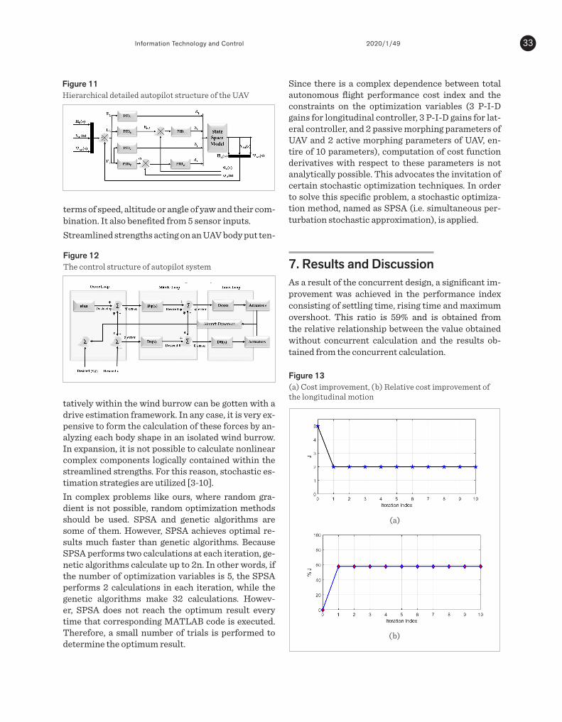
7. Results and Discussion As a result of the concurrent design, a significant improvement was achieved in the performance index consisting of settling time, rising time and maximum overshoot. This ratio is 59% and is obtained from the relative relationship between the value obtained without concurrent calculation and the results obtained from the concurrent calculation.

FFiigguurree 1133 (a) Cost improvement, (b) Relative cost

improvement of the longitudinal motion (a)

(b)

Figure 14 shows the pitch angle of the longitudinal motion, the velocity along the x-

tatively within the wind burrow can be gotten with a drive estimation framework. In any case, it is very ex-pensive to form the calculation of these forces by an-alyzing each body shape in an isolated wind burrow. In expansion, it is not possible to calculate nonlinear complex components logically contained within the streamlined strengths. For this reason, stochastic es-timation strategies are utilized [3-10].In complex problems like ours, where random gra-dient is not possible, random optimization methods should be used. SPSA and genetic algorithms are some of them. However, SPSA achieves optimal re-sults much faster than genetic algorithms. Because SPSA performs two calculations at each iteration, ge-netic algorithms calculate up to 2n. In other words, if the number of optimization variables is 5, the SPSA performs 2 calculations in each iteration, while the genetic algorithms make 32 calculations. Howev-er, SPSA does not reach the optimum result every time that corresponding MATLAB code is executed. Therefore, a small number of trials is performed to determine the optimum result.

Since there is a complex dependence between total autonomous flight performance cost index and the constraints on the optimization variables (3 P-I-D gains for longitudinal controller, 3 P-I-D gains for lat-eral controller, and 2 passive morphing parameters of UAV and 2 active morphing parameters of UAV, en-tire of 10 parameters), computation of cost function derivatives with respect to these parameters is not analytically possible. This advocates the invitation of certain stochastic optimization techniques. In order to solve this specific problem, a stochastic optimiza-tion method, named as SPSA (i.e. simultaneous per-turbation stochastic approximation), is applied.

7. Results and DiscussionAs a result of the concurrent design, a significant im-provement was achieved in the performance index consisting of settling time, rising time and maximum overshoot. This ratio is 59% and is obtained from the relative relationship between the value obtained without concurrent calculation and the results ob-tained from the concurrent calculation.

Figure 13(a) Cost improvement, (b) Relative cost improvement of the longitudinal motion










(b)











(b)


(a)

(b)


Figure 14 Closed-loop responses of longitudinal motion

axis, the angular velocity along the y-axis, the velocity along the z-axis and the responses of the horizontal tail and the elevation angle.

FFiigguurree 1144 Closed-loop responses of longitudinal motion

As can be seen from Figure 14, the longitudinal trajectory has followed the pitch angle well with a little error of 3 degrees. Furthermore, the velocity along the x-axis, the angular velocity along the y-axis followed by the trajectory zero line.

8. Conclusions In this paper, simultaneous longitudinal and lateral flight control systems design for both passive and active morphing unmanned aerial vehicles (UAVs) is first time applied for autonomous flight performance maximization. Dynamic model and longitudinal and lateral state space models of UAV are obtained and then simulation model of UAV is reached. After these, adaptive stochastic optimization method (SPSA), simultaneous design of UAV and autopilot is applied in order to minimize a cost function consisting of rise time, settling time and maximum overshoot. As a result of the concurrent design, a significant improvement was achieved in the performance index consisting of settling time, rising time and maximum overshoot and this ratio is 59%. Since the total cost index captures terms both related with longitudinal and lateral flights, considerable improvement in longitudinal autonomous flight performance was obtained and the lateral autonomous flight performance were not broken. Closed loop responses for both longitudinal and lateral flight while there exist atmospheric turbulence were investigated. The desired trajectories (i.e. 3 degrees roll angle for lateral autopilot and 3 degrees pitch angle for longitudinal autopilot) were successfully tracked. The saturations on active control surfaces (i.e. elevator and aileron) were also satisfied. In addition, the other outputs such as linear and angular velocities were not experienced with catastrophic behavior. Simultaneous design idea converted the UAV and its autopilot system into suitable form satisfying good performance and trajectory tracking for both lateral and longitudinal flights.

References

1. AL-Madani, B., Svirskis, M., Narvydas, G., Maskeliūnas, R., Damaševičius, R. Design of Fully Automatic Drone Parachute System with Temperature Compensation Mechanism for Civilian and Military Applications. Journal of Advanced Transportation, 2018, 1–11. http:// doi.org/10.1155/2018/2964583.

2. Antić, D., Jovanović, Z., Danković, N., Spasić, M., Stankov, S. Probability Estimation of

Figure 14 shows the pitch angle of the longitudinal motion, the velocity along the x-axis, the angular ve-locity along the y-axis, the velocity along the z-axis and the responses of the horizontal tail and the eleva-tion angle.

As can be seen from Figure 14, the longitudinal tra-jectory has followed the pitch angle well with a little error of 3 degrees. Furthermore, the velocity along the x-axis, the angular velocity along the y-axis followed by the trajectory zero line.

8. ConclusionsIn this paper, simultaneous longitudinal and later-al flight control systems design for both passive and active morphing unmanned aerial vehicles (UAVs) is first time applied for autonomous flight performance maximization. Dynamic model and longitudinal and lateral state space models of UAV are obtained and then simulation model of UAV is reached. After these, adaptive stochastic optimization method (SPSA), si-multaneous design of UAV and autopilot is applied in order to minimize a cost function consisting of rise time, settling time and maximum overshoot. As a result of the concurrent design, a significant im-provement was achieved in the performance index consisting of settling time, rising time and maximum overshoot and this ratio is 59%. Since the total cost in-dex captures terms both related with longitudinal and lateral flights, considerable improvement in longitu-dinal autonomous flight performance was obtained and the lateral autonomous flight performance were not broken. Closed loop responses for both longitu-dinal and lateral flight while there exist atmospheric turbulence were investigated. The desired trajecto-ries (i.e. 3 degrees roll angle for lateral autopilot and 3 degrees pitch angle for longitudinal autopilot) were successfully tracked. The saturations on active con-trol surfaces (i.e. elevator and aileron) were also satis-fied. In addition, the other outputs such as linear and angular velocities were not experienced with cata-strophic behavior. Simultaneous design idea convert-ed the UAV and its autopilot system into suitable form satisfying good performance and trajectory tracking for both lateral and longitudinal flights.

References 1. AL-Madani, B., Svirskis, M., Narvydas, G., Maskeliūnas,

R., Damaševičius, R. Design of Fully Automatic Drone Parachute System with Temperature Compensation

Mechanism for Civilian and Military Applications. Journal of Advanced Transportation, 2018, 1-11. https://doi.org/10.1155/2018/2964583

https://doi.org/10.1155/2018/2964583

https://doi.org/10.1155/2018/2964583


2. Antić, D., Jovanović, Z., Danković, N., Spasić, M., Stan-kov, S. Probability Estimation of Certain Properties of the Imperfect Systems. Proceedings of IEEE 7th Inter-national Symposium on Applied Computational Intelli-gence and Informatics, (SACI 2012), Timisoara, Roma-nia, May 24-26, 2012, 213-216. https://doi.org/10.1109/SACI.2012.6250004

3. Bilgic, H. H., Sen, M. A., Kalyoncu, M. Tuning of LQR Controller for an Experimental Inverted Pendulum System Based on the Bees Algorithm. Journal of Vi-broengineering, 2016, 18(6), 3684-3694. https://doi.org/10.21595/jve.2016.16787

4. Brodić, D. Advantages of the Extended Water Flow Algorithm for Handwritten Text Segmentation. In: Kuznetsov, S. O. et al. (Eds.), Pattern Recognition and Machine Intelligence, Lecture Notes in Computer Sci-ence, 6744, Springer, Belin-Heidelberg, 2011, 418-423. https://doi.org/10.1007/978-3-642-21786-9_68

5. Çoban S., Oktay T. A Review of Tactical Unmanned Ae-rial Vehicle Design Studies; The Eurasia Proceedings of Science, Technology, Engineering Mathematics; 2017, (1), 30-35.

6. Çoban S., Oktay T. Legal and Ethical Issues of Un-manned Aerial Vehicles. Journal of Aviation, 2018, 2(1), 31-35. https://doi.org/10.30518/jav.421644

7. Elbanna, A. E. A., Soliman, T. H. M., Ouda, A. N., Hamed, E. M. Improved Design and Implementation of Auto-matic Flight Control System (AFCS) for a Fixed Wing Small UAV. Radioengineering, 2018, 27(3), 882-890. https://doi.org/10.13164/re.2018.0882

8. Gandolfo, D. C., Salinas, L. R., Brandão, A. S., Toibe-ro, J. M. Path Following for Unmanned Helicopter: An Approach on Energy Autonomy Improvement. Infor-

mation Technology and Control, 2016, 45(1), 86-98. https://doi.org/10.5755/j01.itc.45.1.12413

9. Ivanovas, A., Ostreika, A., Maskeliūnas, R., Damaševiči-us, R., Połap, D., Woźniak, M. Block Matching Based Ob-stacle Avoidance for Unmanned Aerial Vehicle. Lecture Notes in Computer Science, 2018, 58-69. https://doi.org/10.1007/978-3-319-91253-0_6

10. Oktay T., Çoban, S. Simultaneous Longitudinal and Lat-eral Flight Control Systems Design For both Passive and Active Morphing Tuavs. Elektronika Ir Elektro-technika, 2017, 23(5), 15-20. https://doi.org/10.5755/j01.eie.23.5.19238

11. Preparata, F. P., Shamos, M. I. Computational Geome-try: An Introduction. Springer, Berlin, 1995.

12. Spall, J. C. Multivariate Stochastic Approximation Us-ing A Simultaneous Perturbation Gradient Approxima-tion. IEEE Transactions on Automatic Control, 1992, 37(3), 332-341. https://doi.org/10.1109/9.119632

13. Tsai, J. L. Efficient Multi-Server Authentication Scheme Based on One-Way Hash Function Without Verification Table. Computers and Security, 2008, 27(3), 115-121. https://doi.org/10.1016/j.cose.2008.04.001

14. Vidojković, B., Jovanović, Z., Milojković, M. The Prob-ability Stability Estimation of the System Based on the Quality of the Components. Facta Universitatis, Se-ries: Electronics and Energetics, 2006, 19(3), 385-391. https://doi.org/10.2298/FUEE0603385V

15. Yazid, E., Garratt, M., Santoso, F. Control Position of A Quadcopter Drone Using Evolutionary Algo-rithms Optimized Self-Tuning 1st-Order Takagi-Su-geno-Kang-Type Fuzzy Logic Controller. Applied Soft Computing, 2019, (1)78, 373-39. https://doi.org/10.1016/j.asoc.2019.02.023

https://doi.org/10.1109/SACI.2012.6250004

https://doi.org/10.1109/SACI.2012.6250004

https://doi.org/10.21595/jve.2016.16787

https://doi.org/10.21595/jve.2016.16787

https://doi.org/10.1007/978-3-642-21786-9_68

https://doi.org/10.30518/jav.421644

https://doi.org/10.13164/re.2018.0882

https://doi.org/10.5755/j01.itc.45.1.12413

https://doi.org/10.1007/978-3-319-91253-0_6

https://doi.org/10.1007/978-3-319-91253-0_6

https://doi.org/10.5755/j01.eie.23.5.19238

https://doi.org/10.5755/j01.eie.23.5.19238

https://doi.org/10.1109/9.119632

https://doi.org/10.1016/j.cose.2008.04.001

https://doi.org/10.2298/FUEE0603385V

https://doi.org/10.1016/j.asoc.2019.02.023

https://doi.org/10.1016/j.asoc.2019.02.023

Documents

Improving Autonomous Performance of a Passive Morphing