Improving Efficiency of PV Systems Using Statistical Performance Monitoring

Report IEA-PVPS T13-07:2017

INTERNATIONAL ENERGY AGENCY PHOTOVOLTAIC POWER SYSTEMS PROGRAMME

Improving Efficiency of PV Systems Using Statistical Performance Monitoring

IEA PVPS Task 13, Subtask 2 Report IEA-PVPS T13-07:2017

June 2017

ISBN 978-3-906042-48-0

Author:

Mike Green (mike@lightning.co.il)

Contributing authors:

Eyal Brill (eyalbrill@decisionmakers.biz)

Birk Jones (cbjones@sandia.gov)

Jonathon Dore (jonathon@solaranalytics.com.au)

3

Table of Contents

Table of Contents ............................................................................................................................... 3

Foreword ............................................................................................................................................ 5

Acknowledgements ............................................................................................................................ 6

List of Abbreviations ........................................................................................................................... 7

Executive Summary ............................................................................................................................ 8

1 Introduction ............................................................................................................................. 10

2 Smart Monitoring of Residential Solar ..................................................................................... 13

2.1 System Inputs.....................................................................................................................13

2.2 Electricity Generation Estimation ......................................................................................14

2.3 Real-Time Monitoring ........................................................................................................14

2.4 Performance Losses ...........................................................................................................14

2.4.1 Shading ..................................................................................................................... 15

2.4.2 Inverter Clipping ....................................................................................................... 15

2.4.3 Power Factor Correction .......................................................................................... 15

2.4.4 String/Module faults ................................................................................................ 16

2.4.5 Excessive Soiling ....................................................................................................... 16

2.4.6 Degradation .............................................................................................................. 16

2.5 Effect of the monitoring resolution ...................................................................................16

2.6 Conclusions ........................................................................................................................19

3 Machine Learning for Fast Fault Recognition........................................................................... 20

3.1 System inputs .....................................................................................................................21

3.2 Theoretical Background .....................................................................................................21

3.3 Results ................................................................................................................................23

3.4 Conclusions ........................................................................................................................28

4 Fault Prediction Using Clustering Algorithms........................................................................... 29

4.1 Theoretical background .....................................................................................................29

4.2 Methodology .....................................................................................................................32

4.3 The test systems ................................................................................................................33

4.4 Results ................................................................................................................................35

4.5 Conclusions ........................................................................................................................36

5 Fault Detection Using Artificial Neural Networks .................................................................... 37

4

5.1 Theoretical background .................................................................................................... 37

5.1.1 Laterally Primed Adaptive Resonance Theory (LAPART) .......................................... 38

5.1.2 Gaussian Process Regression (GPR) .......................................................................... 39

5.1.3 Support Vector Machine (SVM)................................................................................ 39

5.2 Experiments ...................................................................................................................... 40

5.2.1 Maximum Power Point Data .................................................................................... 40

5.2.2 Current & Voltage (I-V) Curve Data .......................................................................... 42

5.3 Results ............................................................................................................................... 43

5.3.1 Maximum Power Point Data .................................................................................... 44

5.3.2 Current & Voltage (I-V) Curve Data .......................................................................... 47

5.4 Conclusions ....................................................................................................................... 49

6 Conclusions ............................................................................................................................... 50

References ........................................................................................................................................ 52

5

Foreword

The International Energy Agency (IEA), founded in November 1974, is an autonomous body within the framework of the Organization for Economic Co-operation and Development (OECD) which carries out a comprehensive programme of energy co-operation among its member countries. The European Union also participates in the work of the IEA. Collaboration in research, develop-ment and demonstration of new technologies has been an important part of the Agency’s Pro-gramme.

The IEA Photovoltaic Power Systems Programme (PVPS) is one of the collaborative R&D Agree-ments established within the IEA. Since 1993, the PVPS participants have been conducting a varie-ty of joint projects in the application of photovoltaic conversion of solar energy into electricity.

The mission of the IEA PVPS Technology Collaboration Programme is: To enhance the internation-al collaborative efforts which facilitate the role of photovoltaic solar energy as a cornerstone in the transition to sustainable energy systems. The underlying assumption is that the market for PV systems is rapidly expanding to significant penetrations in grid-connected markets in an increasing number of countries, connected to both the distribution network and the central transmission network.

This strong market expansion requires the availability of and access to reliable information on the performance and sustainability of PV systems, technical and design guidelines, planning methods, financing, etc., to be shared with the various actors. In particular, the high penetration of PV into main grids requires the development of new grid and PV inverter management strategies, greater focus on solar forecasting and storage, as well as investigations of the economic and technological impact on the whole energy system. New PV business models need to be developed, as the de-centralised character of photovoltaics shifts the responsibility for energy generation more into the hands of private owners, municipalities, cities and regions.

IEA PVPS Task 13 engages in focusing the international collaboration in improving the reliability of photovoltaic systems and subsystems by collecting, analyzing and disseminating information on their technical performance and failures, providing a basis for their technical assessment, and developing practical recommendations for improving their electrical and economic output.

The current members of the IEA PVPS Task 13 include:

Australia, Austria, Belgium, China, Denmark, Finland, France, Germany, Israel, Italy, Japan, Malay-sia, Netherlands, Norway, SolarPower Europe, Spain, Sweden, Switzerland, Thailand and the Unit-ed States of America.

This report focusses on new methods for closely monitoring PV systems by using the existing data produced by the system for statistical analysis. This will enable system owners and maintenance personnel to quickly ascertain a fault condition, even before the fault occurs with some methods, thereby increasing PV system availability.

The editors of the document are Mike Green of M.G.Lightning Ltd, Israel, and Boris Farnung, Fraunhofer ISE, Freiburg, Germany.

The report expresses, as nearly as possible, the international consensus of opinion of the Task 13 experts on the subject dealt with. Further information on the activities and results of the Task can be found at: http://www.iea-pvps.org.

6

Acknowledgements

This report received valuable contributions from several IEA-PVPS Task 13 members and other international experts. Many thanks go to:

Giorgio Belluardo, EURAC research, Institute for Renewable Energy, Italy

David Moser, EURAC research, Institute for Renewable Energy, Italy

Dario Bertani, Ricerca sul Sistema Energetico – RSE S.p.A., Italy

Karl Berger, AIT Austrian Institute of Technology GmbH, Austria

Lyndon Frearson, CAT projects, Australia

Paul Rodden, CAT projects, Australia

This report is supported by the following entities:

Israel Energy and Water Resources Ministry (ISR)

M.G. Lightning Electrical Engineering (ISR)

Decision Makers Ltd. (ISR)

Sandia National Laboratories (USA)

Solar Analytics Pty Ltd (AUS)

7

List of Abbreviations

AC Alternating Current ANN Artificial Neural Networks API Application Programming Interface ART Adaptive Resonance Theory ASL Above Sea Level AUD Australian Dollar CI Confidence Interval DAQ Data Acquisition System DBSCAN Density-Based-Spatial-Clustering of Applications with Noise DC Direct Current EM Expectation-Maximization EPI Energy Performance Index FDD Fault Detection and Diagnostics FN False Negative FOR Forced Outage Rate FP False Positive FPR False Positive Rate GP Gaussian Process GPR Gaussian Process Regression kWh Kilowatt hour kWp Kilowatt peak LAPART Laterally Primed Adaptive Resonance Theory ML Machine Learning MLT Machine Learning Technology MPP Maximum Power Point MPPT Maximum Power Point Tracking NDH Next Day's Hourly Pac Power – Alternating Current PID Potential Induced Degradation POA Plane-Of-Array PPI Power Performance Index PV Photovoltaic ROC Receiver Operating Characteristic RT Regression Tree SVM Support Vector Machine TN True Negative TP True Positive TPR True Positive Rate WWS “WunderGround” Weather Service

8

Executive Summary

Availability, high efficiency and therefore fault detection are of equal importance to the PV sys-tem owner and the grid manager for utility-grade PV and increasingly for the small residential array. With increasing penetration of small arrays, large neighborhoods aggregate to virtual meg-awatt power stations, creating an amorphous and unpredictable power-producing entity.

Achieving and maintaining high efficiency is the responsibility of the system owner. Large PV plants are business units in and of themselves and are managed accordingly. Commercial, small industrial and residential systems are usually erected on independent rooftops with no immediate professional oversight as to daily maintenance. Few small systems are effectively monitored. At best, the system owner monitors the inverter and is made aware of faults to the level of aware-ness that such monitoring is capable of achieving.

The simplicity of the PV system in comparison to other energy-producing systems makes for diffi-cult fault monitoring. Electricity generation in a turbine of any type, for example, entails many moving parts, different pressure levels, changing angles and speeds. Set-points defined for sen-sors on these critical elements in the system can warn of impending system failure. The PV system has only meteorological input and electrical output. No parameters are available for monitoring with a set-point other than the energy readings and the accompanying electrical parameters sup-plied by the electricity generation. Smart meters and new inverter technologies allow monitoring and communications, opening the scope for improved monitoring and analytics at the small sys-tem level. Inverter manufacturers and independent monitoring services supply simple metrics to aid in ascertaining system health such as inverter comparison (when more than one inverter ex-ists) and PR calculation (when irradiance values are available). This report examines four new methods using increasingly advanced statistical analysis of the system-supplied parameters to enable quicker and more exact alerts, particularly for the residential system maintained by non-professionals. By being technology independent, the methods have applications for grid-level integration of distributed energy.

The first system for residential solar analytics was developed in Australia, where solar irradiation data is made available free of charge by the government. This system comprises a simple energy meter installed on the PV system feed into the electrical power-distribution box that collects data. Using statistical analysis, the data on generated electricity is compared to an expected generation profile from the irradiation data and system configuration. The system owner has access to real-time electricity generation data and fault diagnosis that identifies issues and what to check if per-formance was not as expected.

The second system uses machine learning to predict next day’s hourly production by small resi-dential systems for aggregation into virtual neighborhood power plants for the benefit of grid managers. This system requires only inverter data feed to the system server. The algorithms work on the inverter feed and meteorological prediction extracted from commercially available mete-orological servers. No irradiation data or system configuration data is required. Applying these algorithms on yesterday’s weather history, as opposed to weather predictions, produces an im-mediate indication of system health. Tracking daily system health, which is simplified to qualita-tive ratings from A to F, enables even the smallest system to positively ascertain that the system is performing as expected or that a service call should be made.

Fault prediction is the topic of the third system described in this report, which is also based on machine-learning algorithms. Clustering statistical methods are used to predict future faults that will affect power production. This system requires only an inverter data feed and access to histor-ical meteorological data extracted from commercially available meteorological servers. No irradia-tion data or system configuration data is required. This system has proven so far to predict future

9

loss due to faults, though work continues to classify the specific fault that will occur in order to enable the owner to undertake appropriate preemptive corrective action.

The last system to be described in this report demonstrates promising application of artificial neu-ral networks. These algorithms learn the behavior of the system from the available inputs. This learned behavior is compared to incoming real-time parameters from the system, enabling detec-tion of faults much faster than existing methods in the field today such as Performance Ratio, Power Performance Index or inverter comparison, for example. At the time of writing, the devel-oped algorithms have produced good results in the test systems. Future work requires that the algorithms be applied to data from various seasons and locations and combined with more testing and development to detect a wider variety of fault conditions.

10

1 Introduction

PV systems have come of age to the extent that PV energy penetration into national electrical grid systems has reached double digit percentages of total electricity generation in some countries. Grid-connected PV electricity generation began on the residential roof top, augmenting electricity generation while following a healthy grid, and shutting down when the distribution grid left ac-ceptable parameters for voltage or frequency. From residential systems of a few kilowatts in size, PV arrays grew to commercial systems of tens and hundreds of kilowatts, then progressed to utili-ty-grade PV power stations of tens of megawatts. Small residential systems in some neighbor-hoods aggregate to virtual power plants of some megawatts in size, while utility-grade PV power plants in some countries are no longer allowed to shut down when the grid is stressed, but must support the grid, producing reactive energy to aid in grid stabilization.

Utility-grade PV power plants are growing in size, yet residential PV systems outstrip them in most countries, certainly in number and even in total installed capacity. The utility-grade PV plant is increasingly being treated as a conventional power plant and the developers/owners of these industrially sized and maintained plants can negotiate with the utilities on mutually accepted terms that meet the business plan of both parties. Residential PV, however, leaves the utility with many challenges. Before the advent of the current popularity of PV in the residential market, resi-dents would purchase a certain amount of electrical energy from a given utility. At some point the residents began installing PV systems on their roof tops. The utility now sells less energy to these household, decreasing profits. However, these PV systems produce electricity by the whims of the weather, creating uncertainty in the amount of reserve energy the utility grid manager must have on hand at any given time, requiring higher levels of spinning reserve. The utility faces new chal-lenges in meeting uncertain demand with uncertain supply and tighter constraints on voltage and frequency control.

The loss of revenue due to distributed generation, which requires regulators to rethink tariff sys-tems to reflect the evolving modern distribution grid that includes distributed generation, cannot be dealt with in the scope of this report. However, challenges with integrating distributed energy generation can be reduced using the methods reported here, by enabling the utility grid manager to better forecast electricity generation from residential neighborhoods, and by greatly increasing the availability and lowering Forced Outage Rate (FOR) of the neighborhood as a virtual multi-megawatt power plant.

From the point of view of the system owner, low availability and low efficiency translate directly to loss of revenue even more so than for the grid manager, particularly for larger systems under scrutiny from financial agencies demanding performance reviews that match expectations. Early fault detection enables the system owner to act quickly to repair the fault, thereby retaining effi-ciency, and could prevent excessive abnormal behavior that can lead to major damage including fire and electric shock.

Early monitoring of PV systems encompassed the simple collection of parameters such as power, voltage, current, etc., from the inverter. Different inverter manufacturers offered different data sets. As systems grew to commercial sizes with business plans under commercial scrutiny, solar irradiation sensors became more common, enabling the calculation of a performance ratio to enable system owners to understand the overall efficiency of their systems. Professional suppliers of monitoring services can now plot the power produced against the solar irradiation in real time.

In systems consisting of more than one inverter, it has become common for monitoring services to supply a daily comparison of the inverters in the system. Since in many systems the inverters are not all of the same size, and even when of the same size they are not always loaded with the same number of modules on the DC side, the monitoring service must first normalize the parame-

11

ters to be used. This normalization is the ratio of the parameter in use to the area of PV modules measured in square meters, producing a value for a single square meter, or to the installed power of the modules. The normalized parameter is then easily compared to that from other inverters.

Monitoring for large systems [1] with larger budgets that are funded by financial institutions is backed by the financial capacity and the motivation to install more complex monitoring hardware elements such as string monitoring, coupled with custom monitoring software. This combination enables alarms on low-producing strings or the use of weather-corrected performance ratio met-rics [2] that offer a more accurate performance ratio based on module temperature as well as solar irradiation. As a result, all large PV installations are typically well monitored for efficiency and availability, enabling early detection of fault conditions or low efficiency.

Until recently however, for small residential systems there has not been a cost-effective solution for monitoring and fault detection. As a result, the reality for small-system efficiency is that faults are often not discovered for some weeks or months, usually after the delivery and analysis of the monthly or quarterly electric bill.

Unlike utility-scale or large commercial systems, the cost of monitoring for single-inverter systems has been prohibitive. With independent single inverters, as for a large percentage of residential systems, it has not been possible to do an inverter comparison, performance ratio calculation or any other metric showing that the system could be producing more than it did. This reality has led many small-system owners to have no monitoring at all, since simple, cost-effective methods for ascertaining system health were not available.

With smart metering, new inverter technologies and cloud-based data sharing, new opportunities for smart monitoring of residential solar installations are emerging. This report will describe four methods for statistical analysis of the parameters supplied by a PV system that will enable system owners to understand their system performance better and to identify whether and when their system is losing revenue. At the same time, monitoring can indicate a risk of impending faults, thereby increasing availability, and inform the grid manager of intermittent supply, reducing the Forced Outage Rate and increasing predictability.

This report attempts to show a departure from classic system monitoring based on comparing system parameters to sensor outputs or the dependence on relatively costly service-based meth-ods for detecting dropping efficiency, towards dependence on readily available system parame-ters and their statistical relativity. Four methodologies are described, arguably from the least to greatest mathematical complexity. The order does represent the development chronology, with the first system being developed earlier than the rest and consequently being longer in the field; the last system described is still in the academic stages.

The first methodology is described by Jonathan Dore, of the Australian company Solar Analytics Pty. This system was developed in Australia primarily for residential solar analytics, where about 98 % of the almost 1.6 million solar systems installed on the continent are residential or commer-cial and under 10kWp in size [3]. The addition of a simple monitoring device mounted in the resi-dential electrical distribution box, along with weather data combined with the system configura-tion, enables the use of statistical algorithms to detect fault conditions quickly.

The second method to be discussed is described by Mike Green of the Israeli company M.G.Lightning Ltd. This method was developed with the intended purpose of accurately predict-ing the next-day hourly yield of residential and commercial systems using energy or power pa-rameters from the existing inverter data loggers and inexpensive hourly meteorological predic-tions from nearby public weather servers containing no irradiation data. These algorithms, when used on the historical data from the same meteorological server for the finished production day, will inform the system owner of the system health, enabling the system owner to react quickly to a failing or failed system.

12

The third method to be discussed is also described by Mike Green of the Israeli company M.G.Lightning Ltd. This system works to predict faults before they occur, using clustering ma-chine-learning algorithms applied to system-produced parameters retrieved from the existing inverter data loggers, inexpensive hourly meteorological predictions from nearby public weather servers containing no irradiation data and a variety of system-specific calculated values. These new algorithms predict the on-coming of a fault condition that will cause loss of revenue. Contin-ued work on these algorithms should enable the prediction to be expanded to include the type of fault and a timeline for the future fault.

The fourth system is described by Birk Jones of Sandia National Laboratories of the United States. It is an academic portrayal of initial work done using Artificial Neural Networks to enable fast, almost immediate detection of faults by learning the behavior of the system from the available inputs, and producing a behavior pattern to which incoming parameters are compared. If the incoming data from the PV system are not within the learned behavior parameters, a fault is ap-parent. Three types of algorithms were developed and tested with good results.

It is apparent from the four systems described in this report from three research and develop-ment centers, which are independent of each other and situated equally across 17 time zones, each serving their perceived market, that the state of the art for monitoring PV systems is moving from a sensor-based system to one of statistical calculations performed on system production parameters. This development comes about due to the granular nature of PV electricity genera-tion in a national grid. The total PV electricity generated in a national grid is largely supplied by many small systems with small financial plans that cannot support high-efficiency monitoring on their own. Statistical analysis requires no hardware, so the cost of the monitoring is flexible.

As the world moves towards distributed generation with multi-directional power flow within dis-tribution grids, these statistical methods will become crucial to retain efficiency and predict the electricity yield.

13

2 Smart Monitoring of Residential Solar

Jonathan Dore Australia

At time of writing, the PV market in Australia includes close to 1.6 million PV systems, 98 % of them rooftop systems with less than 10 kWp of installed power [4]. This amount of PV energy injected into the grid creates many challenges to the grid operators. This great uptake of rooftop PV by residential grid customers in Australia is a result of a combination of high irradiance, sup-portive policy and residential electricity prices averaging AUD 0.21 to 0.38/kWh and peaking at AUD 0.50/kWh.

With more than 20 % of residential households generating power from their rooftops, there is a significant investment and influence on the grid that would benefit from monitoring. With stand-ard installed hardware, small-system owners are not able to monitor or predict yield with any accuracy or at all.

In Australia, satellite irradiance and weather data are available from the national weather service free of charge. This available information coupled with accurate readings of the energy feed at the level of the residential electric power-meter box enables some powerful statistical calcula-tions that can aid the system owner to quickly determine that their system is not producing as it should.

Motivated by feed-in tariffs or self-consumption, the system owner has a strong interest in learn-ing of faults as soon as possible to ensure expected revenue from the system. Methods used for fault detection in small systems, where no irradiation sensors exist, depend primarily on assump-tions as to what the system should be producing. Accuracy of these estimates is improved by comparing with production estimates based on weather and nearby system data. The statistical tools described here use both available irradiance and weather data and the behavior of the plant itself to ascertain normal behavior, and to understand what is wrong when behavior is abnormal.

2.1 System Inputs

The system owner or installer is responsible for supplying the system parameters such as:

Location PV module type Inverter type PV module orientation PV module tilt String configuration

Additional monitoring hardware is added to the system, as shown in Figure 1, to acquire the elec-trical parameters from the inverter. The acquired parameters available for statistical analysis in-clude:

Current Voltage Frequency Active energy over 5 seconds Reactive energy over 5 seconds

14

Figure 1: AC Power data from the inverter is acquired by a monitor mounted in the power meter box

Meteorological data and satellite irradiance maps are supplied by the national weather service. Temperature and wind-speed are supplied in 30-minute intervals. The irradiance data is supplied as a daily aggregate of satellite-derived global horizontal irradiance

2.2 Electricity Generation Estimation

The daily irradiance data is further manipulated using algorithms developed in collaboration with the University of New South Wales for:

temporal irradiance separation direct/diffuse irradiance separation plane-of-array irradiance transposition

Using these algorithms, an hourly plane-of-array irradiance is calculated for each hour of the day.

The one-sun power of the specified modules is de-rated according to the available plane-of-array irradiance and then a temperature de-rating is applied as a function of manufacturer-specified temperature coefficients, ambient temperature, wind-speed, mounting configuration and irradi-ance.

The expected module power is then aggregated across each string in the system to obtain a total DC power for a given inverter input. The AC power is then calculated, applying a further de-rating based on manufacturer-specified inverter efficiency and limited by maximum inverter output.

The power is calculated for the mid-point of each hour and used as an average to calculate the generated electricity for that hour.

2.3 Real-Time Monitoring

The PV generation is assessed every hour to determine if the site is online and producing. If the power is negligible, an alarm is sent to the system owner.

At the end of each day, the daily energy generation is compared with the values calculated from the system parameters. If the performance is lower than expected, diagnostic algorithms are run and an alert is sent.

2.4 Performance Losses

Diagnostics are run on the system when the production is lower than the calculated production values. The analytics then compares the fault signal with known fault signatures to identify the likely cause of the underperformance. Some examples of fault finding include:

15

2.4.1 Shading

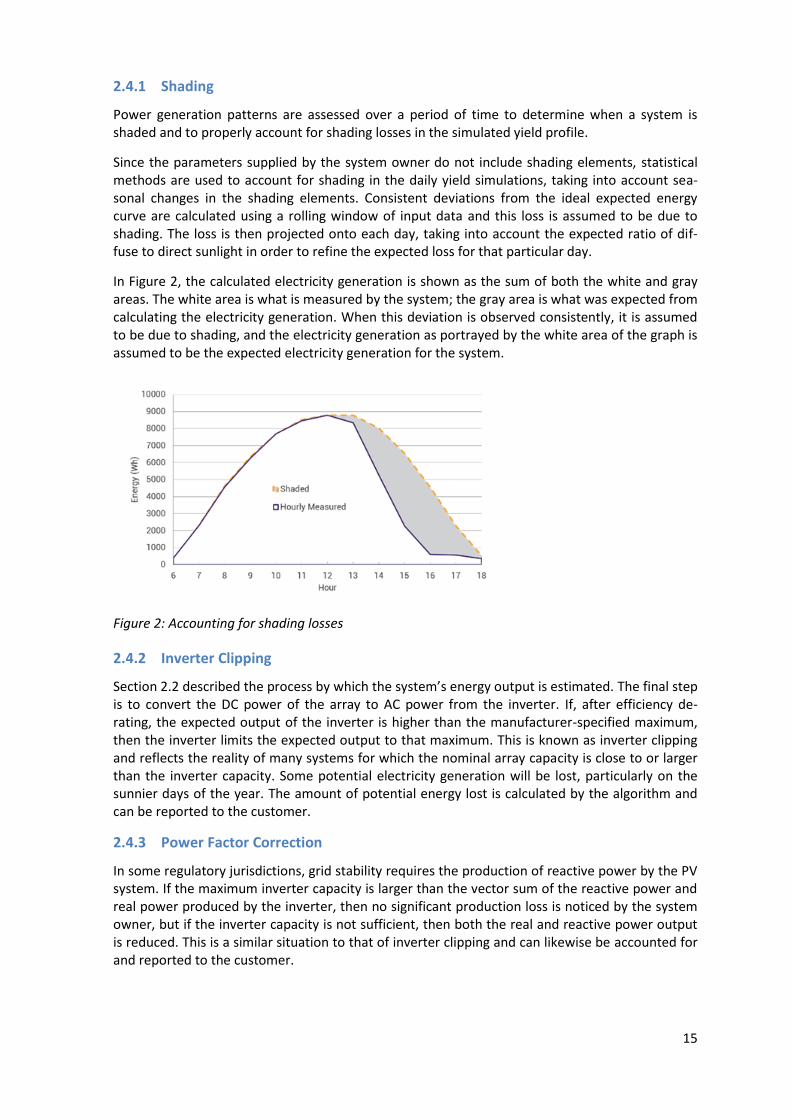
Power generation patterns are assessed over a period of time to determine when a system is shaded and to properly account for shading losses in the simulated yield profile.

Since the parameters supplied by the system owner do not include shading elements, statistical methods are used to account for shading in the daily yield simulations, taking into account sea-sonal changes in the shading elements. Consistent deviations from the ideal expected energy curve are calculated using a rolling window of input data and this loss is assumed to be due to shading. The loss is then projected onto each day, taking into account the expected ratio of dif-fuse to direct sunlight in order to refine the expected loss for that particular day.

In Figure 2, the calculated electricity generation is shown as the sum of both the white and gray areas. The white area is what is measured by the system; the gray area is what was expected from calculating the electricity generation. When this deviation is observed consistently, it is assumed to be due to shading, and the electricity generation as portrayed by the white area of the graph is assumed to be the expected electricity generation for the system.

Figure 2: Accounting for shading losses

2.4.2 Inverter Clipping

Section 2.2 described the process by which the system’s energy output is estimated. The final step is to convert the DC power of the array to AC power from the inverter. If, after efficiency de-rating, the expected output of the inverter is higher than the manufacturer-specified maximum, then the inverter limits the expected output to that maximum. This is known as inverter clipping and reflects the reality of many systems for which the nominal array capacity is close to or larger than the inverter capacity. Some potential electricity generation will be lost, particularly on the sunnier days of the year. The amount of potential energy lost is calculated by the algorithm and can be reported to the customer.

2.4.3 Power Factor Correction

In some regulatory jurisdictions, grid stability requires the production of reactive power by the PV system. If the maximum inverter capacity is larger than the vector sum of the reactive power and real power produced by the inverter, then no significant production loss is noticed by the system owner, but if the inverter capacity is not sufficient, then both the real and reactive power output is reduced. This is a similar situation to that of inverter clipping and can likewise be accounted for and reported to the customer.

16

2.4.4 String/Module faults

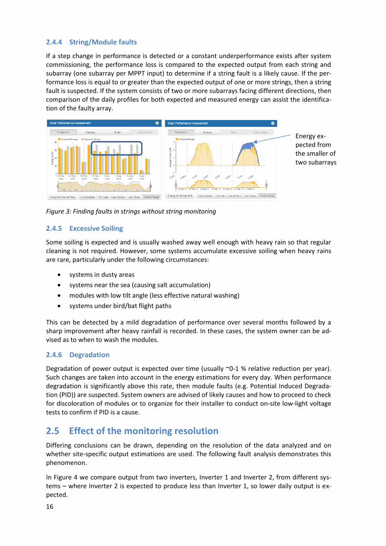
If a step change in performance is detected or a constant underperformance exists after system commissioning, the performance loss is compared to the expected output from each string and subarray (one subarray per MPPT input) to determine if a string fault is a likely cause. If the per-formance loss is equal to or greater than the expected output of one or more strings, then a string fault is suspected. If the system consists of two or more subarrays facing different directions, then comparison of the daily profiles for both expected and measured energy can assist the identifica-tion of the faulty array.

Figure 3: Finding faults in strings without string monitoring

2.4.5 Excessive Soiling

Some soiling is expected and is usually washed away well enough with heavy rain so that regular cleaning is not required. However, some systems accumulate excessive soiling when heavy rains are rare, particularly under the following circumstances:

systems in dusty areas

systems near the sea (causing salt accumulation)

modules with low tilt angle (less effective natural washing)

systems under bird/bat flight paths

This can be detected by a mild degradation of performance over several months followed by a sharp improvement after heavy rainfall is recorded. In these cases, the system owner can be ad-vised as to when to wash the modules.

2.4.6 Degradation

Degradation of power output is expected over time (usually ~0-1 % relative reduction per year). Such changes are taken into account in the energy estimations for every day. When performance degradation is significantly above this rate, then module faults (e.g. Potential Induced Degrada-tion (PID)) are suspected. System owners are advised of likely causes and how to proceed to check for discoloration of modules or to organize for their installer to conduct on-site low-light voltage tests to confirm if PID is a cause.

2.5 Effect of the monitoring resolution

Differing conclusions can be drawn, depending on the resolution of the data analyzed and on whether site-specific output estimations are used. The following fault analysis demonstrates this phenomenon.

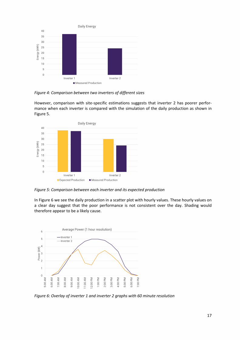
In Figure 4 we compare output from two inverters, Inverter 1 and Inverter 2, from different sys-tems – where Inverter 2 is expected to produce less than Inverter 1, so lower daily output is ex-pected.

Energy ex-pected from the smaller of two subarrays

17

Figure 4: Comparison between two inverters of different sizes

However, comparison with site-specific estimations suggests that inverter 2 has poorer perfor-mance when each inverter is compared with the simulation of the daily production as shown in Figure 5.

Figure 5: Comparison between each inverter and its expected production

In Figure 6 we see the daily production in a scatter plot with hourly values. These hourly values on a clear day suggest that the poor performance is not consistent over the day. Shading would therefore appear to be a likely cause.

Figure 6: Overlay of inverter 1 and inverter 2 graphs with 60 minute resolution

18

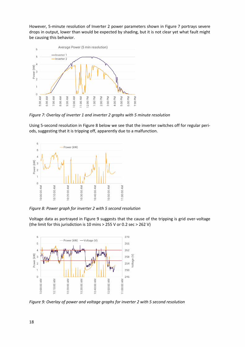
However, 5-minute resolution of Inverter 2 power parameters shown in Figure 7 portrays severe drops in output, lower than would be expected by shading, but it is not clear yet what fault might be causing this behavior.

Figure 7: Overlay of inverter 1 and inverter 2 graphs with 5 minute resolution

Using 5-second resolution in Figure 8 below we see that the inverter switches off for regular peri-ods, suggesting that it is tripping off, apparently due to a malfunction.

Figure 8: Power graph for inverter 2 with 5 second resolution

Voltage data as portrayed in Figure 9 suggests that the cause of the tripping is grid over-voltage (the limit for this jurisdiction is 10 mins > 255 V or 0.2 sec > 262 V)

Figure 9: Overlay of power and voltage graphs for inverter 2 with 5 second resolution

19

2.6 Conclusions

Monitoring of residential solar PV generation, combined with statistical evaluation of the data enables the system owner to acquire real-time data and in-depth analysis of the system health, based on a comparison between the predicted hourly production and the actual monitored pro-duction.

The system depends on the ability to simulate the day’s production based on solar irradiation data and the monitoring of the AC energy input to the local electrical power-distribution box.

The system owner has only to install the modular data monitor in the electrical power-distribution box and to describe the PV system configuration in a web-based input form. The cloud-based monitoring system collects the energy data and acquires the irradiation and meteorological data for the day past, then performs the simulation.

The algorithms complete the simulation of the electricity generation by statistically comparing the actual yield with the simulation and correcting for shading and other elements that cannot be input by the owner.

The algorithms are applied to a profile of the system that enables an understanding of unusual behavior and the consequent classification of this behavior as a solvable problem, such as loss of string production in an MPPT input.

High-resolution data, recorded at intervals down to 5 seconds, is stored for analyzing the cause of any loss of revenue that may be found by this monitoring system.

20

3 Machine Learning for Fast Fault Recognition

Mike Green and Eyal Brill Israel

This method was developed with the intended purpose of accurately predicting the Next Day’s Hourly (NDH) yield of residential and commercial systems using existing inverter data loggers and inexpensive hourly meteorological predictions from nearby public weather servers.

Before the “Solar Boom”, grid managers knew exactly how much power was to be delivered every hour the next day by each power plant on the grid. The grid manager would also pay for some generators to run without producing energy, as a spinning reserve to be used if the consumption changed from that forecast.

As PV energy becomes more common, the uncertainty increases, requiring more expensive spin-ning reserve. Utilities and regulators can insist that large, industrial-sized PV plants pay for predic-tion services based on irradiation maps and hourly simulations, even incurring penalties if the prediction is incorrect. This is not possible in the case of the small residential PV system owner. These systems, usually under 10 kWp in size, are not equipped with the hardware or software to enable accurate predictions and for the most part, irradiation maps are not available. However, some neighborhoods have become multi-megawatt PV power stations, with many tens of sepa-rate systems each consisting of different combinations of inverters, modules, orientations, inclina-tions and even functionality.

Unlike the case of large commercial systems, a large neighborhood system aggregated of many small systems is characterized by large variability of daily results when compared to the theoreti-cal results. This is mainly due to two reasons. First, small systems are affected by any change of conditions, the difference between individual locations is large and this yields a difference in pro-duction. Second, the quality of maintenance is not the same for all systems. As a result of this variability a theoretical model which fits all systems is not applicable. If one would like to achieve daily prediction with high accuracy in spite of the above conditions, a different approach must be taken.

One of the possible approaches uses Machine Learning Technology (MLT). The MLT is a set of mathematical algorithms which “learns” the relation between past inputs and outputs of a system and tries to predict future outputs based on future inputs. It is important to note that the result of the “learning” process is a specific relationship for each system. This specific relation is called “a model”. A model of a system in this case is “Inverter-based”. Thus it reflects the specific condition under which the inverter is working (e.g. geographic location, weather, tilt, azimuth, etc.). It also reflects the specific hardware characteristics of each inverter. If for example two originally identi-cal inverters (i.e. produced by the same manufacturer at the same time) receive different mainte-nance, the result should be reflected in the model.

As explained in Chapter 3.2, the MLT described uses a “Regression Tree” (RT). The RT uses only the power or energy parameters from the inverter data logger and meteorological predicted data available from public weather servers.

Since the system can accurately predict the NDH yield, these algorithms, when applied to the historical data acquired from the same weather server at the same time as next day’s predictions, can ascertain if the system performed as it should have. If not, the system owner can be notified to examine the system.

21

3.1 System inputs

The only required input from the system owner is hourly energy or power parameters from the inverter.

From an online weather server near the PV system, the following parameters are collected from today’s hourly historical data and tomorrow’s hourly predictions:

Temperature Humidity Barometric pressure Wind speed Dew point Rain Sky view (amount of sky covered by clouds)

All variables are continuous variables except the last one, which is a category variable that de-scribes the sky state (clear, partial cloudy, cloudy, rain, fog etc.).

The service that was used in the development of these algorithms is the “WunderGround” Weather Service (WWS). This a low-cost service with open Application Programming Interface (API) which gives easy access to real historical data and future weather prediction based on hourly results.

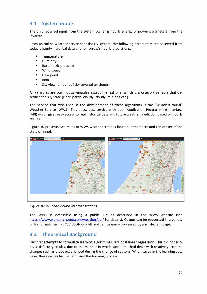
Figure 10 presents two maps of WWS weather stations located in the north and the center of the state of Israel.

Figure 10: WunderGround weather stations.

The WWS is accessible using a public API as described in the WWS website (see https://www.wunderground.com/weather/api/ for details). Output can be requested in a variety of file formats such as CSV, JSON or XML and can be easily processed by any .Net language.

3.2 Theoretical Background

Our first attempts to formulate learning algorithms used local linear regression. This did not sup-ply satisfactory results, due to the manner in which such a method dealt with relatively extreme changes such as those experienced during the change of seasons. When saved in the learning data base, these values further confused the learning process.

22

As was indicated in the previous section, a regression tree was found to offer good results; the longer the learning period, the better the results. In this section, a short theoretical description of the Regression Tree (RT) is given.

The idea behind the RT is to divide multi-dimensional hyperspace into small subspaces and to create for each subspace a linear (or non-linear) model which creates a prediction in the immedi-ate surrounding only. The use of this approach allows for inputs and outputs to have different relationships in different subspaces. For example, wind acts to cool the PV modules; however humidity affects the heat transfer. Since humidity, wind speed and ambient temperature affect the back module temperature; different changes in these inputs may have different results de-pending on the conditions. Thus, a different model should be constructed for each set of condi-tions.

The main question is how to generate the subspaces and what type of model (linear or nonlinear) should be used in each subspace.

Theoretically there are several options for efficiently splitting a multi-dimensional space into sub-spaces. One of the main options is to use a measurement quantity called “entropy”. The entropy is measured by the following equation:

])[(log)()(1

N

i

b xxPxEntropy

When the distribution is continuous rather than discrete, the sum is replaced by an integral as follows:

dxxPxPxEntropy b ])([log)()(

In the case where the dependent variable (energy) is a continuous variable (as in our case), the target of the tree builder should be variance reduction instead of an entropy reduction. The vari-ance reduction of a node N is defined as the total reduction of the variance of the target (de-pendent) variable (energy) due to the split at this node. Variance is calculated as the sum of squared differences between the value of each record and the mean. In our case we use the me-dian instead of the mean.

N

i

ixN

xVariance1

2)(1

)(

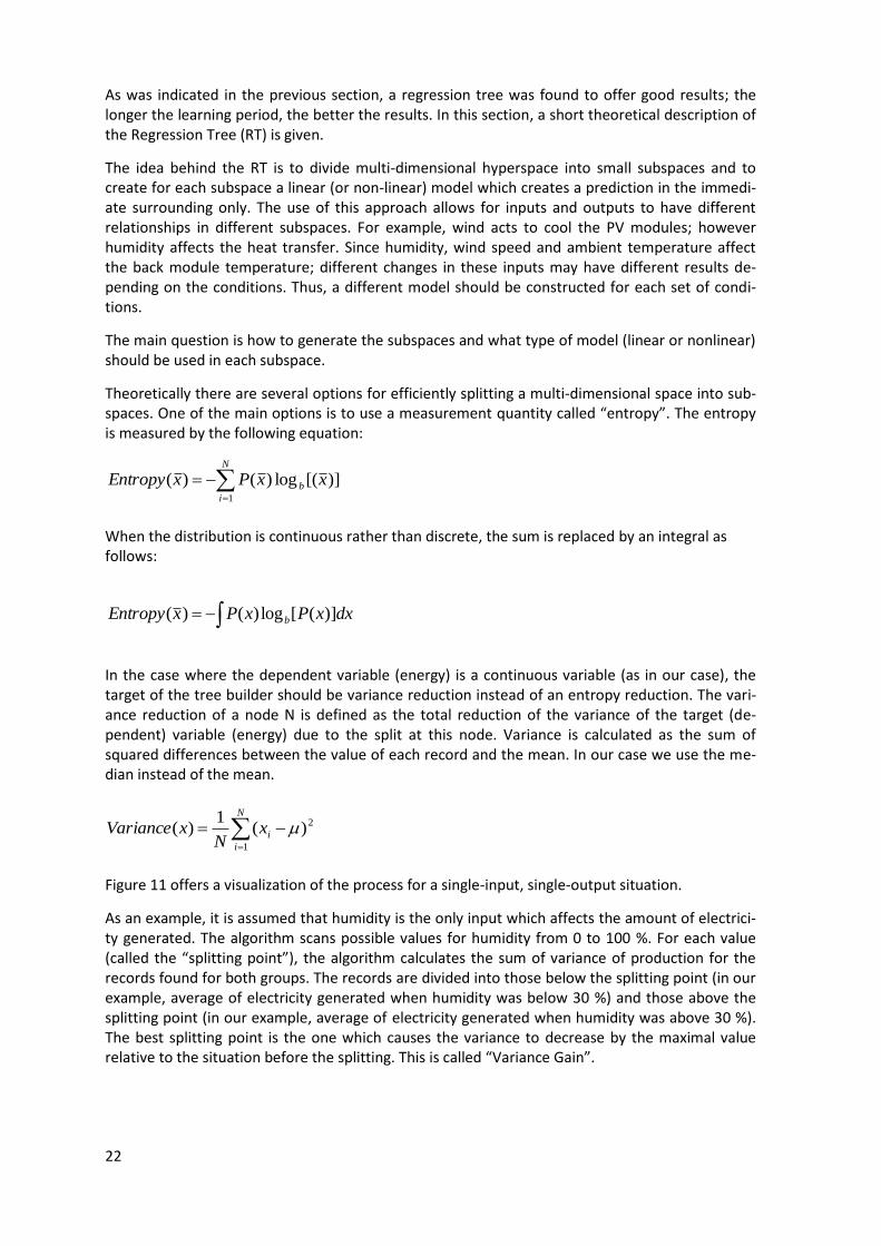
Figure 11 offers a visualization of the process for a single-input, single-output situation.

As an example, it is assumed that humidity is the only input which affects the amount of electrici-ty generated. The algorithm scans possible values for humidity from 0 to 100 %. For each value (called the “splitting point”), the algorithm calculates the sum of variance of production for the records found for both groups. The records are divided into those below the splitting point (in our example, average of electricity generated when humidity was below 30 %) and those above the splitting point (in our example, average of electricity generated when humidity was above 30 %). The best splitting point is the one which causes the variance to decrease by the maximal value relative to the situation before the splitting. This is called “Variance Gain”.

23

Figure 11: Principle of variance gain calculation

The algorithm scans all variables, calculating the best splitting point for each variable. Then the variance reduction from all variables is examined to choose the variable which reduces the varia-bility the most. This variable supplies us with the first splitting point

Once the first splitting point has been selected, the process continues for each sub-group sepa-rately and recursively, taking into account only the records in each group. The process ends when all sub-groups generated have a uniform output value or the number of records in the group is less than a predefined value; for example, 100 records. We shall call the final results of the sub-groups “leaves” (a single one is a leaf).

Since the inputs include both continuous and discrete variables, both entropy reduction and vari-ance reduction are used respectively for the splitting process.

Once the multi-dimensional space has been reduced into subspaces (leaves), for each leaf the algorithm calculates a linear equation between the output (energy) and several inputs.

In case the process of estimating the linear equation for a given leaf fails or produces a linear es-timation of low quality, the median of output (energy) of all records in this leaf is used instead. Using the median is more robust than using the mean since the median is more immune to outli-ers.

The resulting regression tree is saved to a file for later use. During prediction, the following pro-cess occurs:

Using the inputs for a requested prediction, the algorithm locates the relevant leaf in the tree

It then assigns the input values to the equation of the leaf to generate a prediction In case the prediction is more than 3 standard deviations from the median, the median is

used as the output and not the regression result

3.3 Results

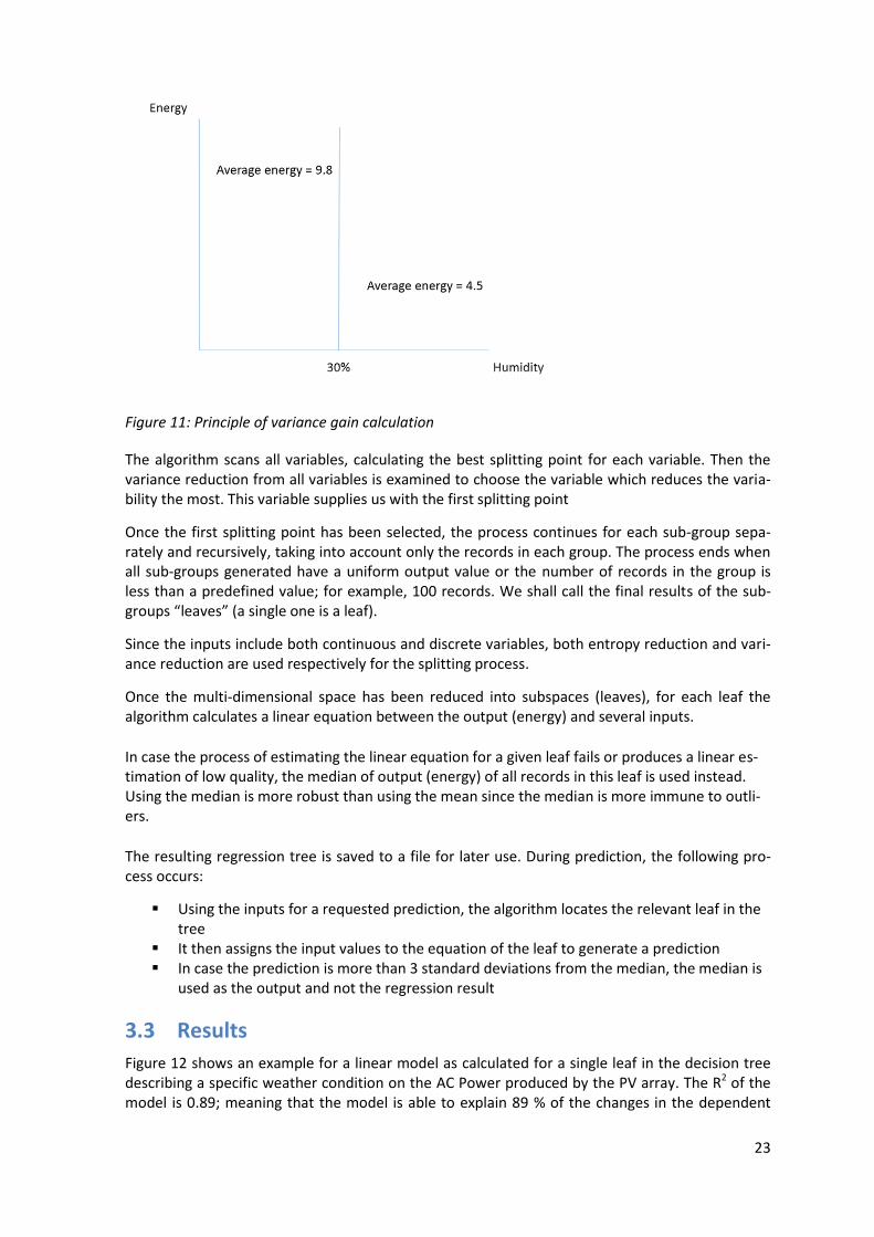
Figure 12 shows an example for a linear model as calculated for a single leaf in the decision tree describing a specific weather condition on the AC Power produced by the PV array. The R2 of the model is 0.89; meaning that the model is able to explain 89 % of the changes in the dependent

24

variable (AC power). The F value is 85.295 with probability < 0.001; meaning that the probability that the model missed an explanatory variable is less than 0.001 percent, these two values make the model significant. The entire list of coefficients for the variables is significant, with a P value less than 0.001. The P value of each coefficient (for a variable) is the probability that this variable will have no effect on the dependent variable (AC Power) and should therefore not be included in the model. As can be seen for all variables the probability for such a case is less than 0.001.

The values in the “Parameter Estimates” of Figure 12 are the coefficients of the linear model that should be used for prediction.

Figure 12: Example for linear model results

The following examples are of next day hourly predictions based on weather predictions, not his-torical values. The algorithms applied to historical meteorological values for the purpose of fault detection are more accurate to the degree of the weather prediction accuracy.

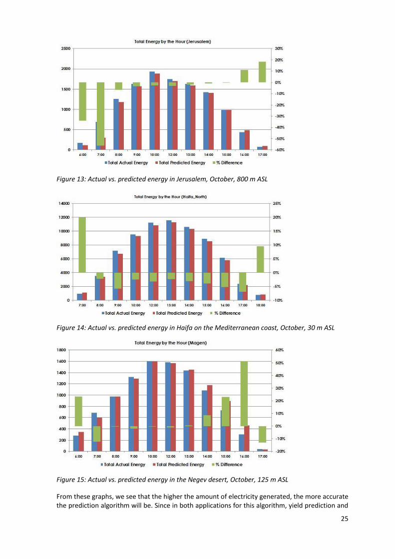
The following set of graphs portrays the algorithm`s performance after about one year in the field. As explained previously, the longer the algorithms are in use, the more accurate they be-come. These graphs present the hourly aggregation for the month of October, a month notable for seasonal changes. The three systems shown are each in a different climatic area. Figure 13 shows the electricity generated and predicted from Jerusalem, at 800 m Above Sea Level (ASL). Figure 14 presents the values from the Haifa coast, some tens of meters from the sea and at an elevation of about 30 m ASL. Figure 15 portrays a system in the Negev desert at an elevation of 125 m ASL.

25

Figure 13: Actual vs. predicted energy in Jerusalem, October, 800 m ASL

Figure 14: Actual vs. predicted energy in Haifa on the Mediterranean coast, October, 30 m ASL

Figure 15: Actual vs. predicted energy in the Negev desert, October, 125 m ASL

From these graphs, we see that the higher the amount of electricity generated, the more accurate the prediction algorithm will be. Since in both applications for this algorithm, yield prediction and

26

as an indicator of system health, the emphasis is on times of high electricity output, it may be possible to filter or ignore the early morning and late afternoon.

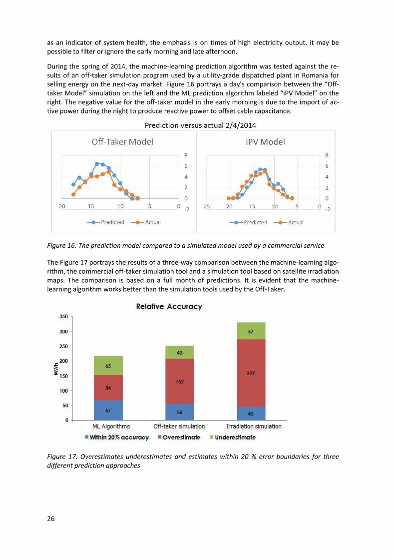
During the spring of 2014, the machine-learning prediction algorithm was tested against the re-sults of an off-taker simulation program used by a utility-grade dispatched plant in Romania for selling energy on the next-day market. Figure 16 portrays a day’s comparison between the “Off-taker Model” simulation on the left and the ML prediction algorithm labeled “iPV Model” on the right. The negative value for the off-taker model in the early morning is due to the import of ac-tive power during the night to produce reactive power to offset cable capacitance.

Figure 16: The prediction model compared to a simulated model used by a commercial service

The Figure 17 portrays the results of a three-way comparison between the machine-learning algo-rithm, the commercial off-taker simulation tool and a simulation tool based on satellite irradiation maps. The comparison is based on a full month of predictions. It is evident that the machine-learning algorithm works better than the simulation tools used by the Off-Taker.

Figure 17: Overestimates underestimates and estimates within 20 % error boundaries for three different prediction approaches

27

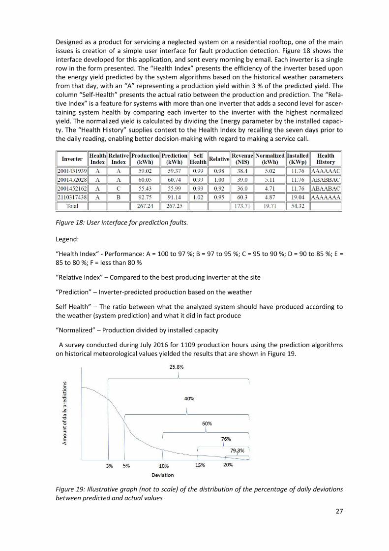
Designed as a product for servicing a neglected system on a residential rooftop, one of the main issues is creation of a simple user interface for fault production detection. Figure 18 shows the interface developed for this application, and sent every morning by email. Each inverter is a single row in the form presented. The “Health Index” presents the efficiency of the inverter based upon the energy yield predicted by the system algorithms based on the historical weather parameters from that day, with an “A” representing a production yield within 3 % of the predicted yield. The column “Self-Health” presents the actual ratio between the production and prediction. The “Rela-tive Index” is a feature for systems with more than one inverter that adds a second level for ascer-taining system health by comparing each inverter to the inverter with the highest normalized yield. The normalized yield is calculated by dividing the Energy parameter by the installed capaci-ty. The “Health History” supplies context to the Health Index by recalling the seven days prior to the daily reading, enabling better decision-making with regard to making a service call.

Figure 18: User interface for prediction faults.

Legend:

“Health Index“ - Performance: A = 100 to 97 %; B = 97 to 95 %; C = 95 to 90 %; D = 90 to 85 %; E = 85 to 80 %; F = less than 80 %

“Relative Index” – Compared to the best producing inverter at the site

“Prediction” – Inverter-predicted production based on the weather

Self Health” – The ratio between what the analyzed system should have produced according to the weather (system prediction) and what it did in fact produce

“Normalized” – Production divided by installed capacity

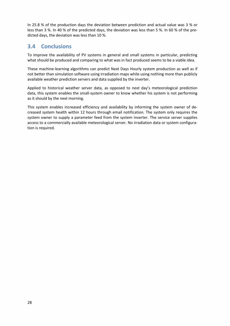
A survey conducted during July 2016 for 1109 production hours using the prediction algorithms on historical meteorological values yielded the results that are shown in Figure 19.

Figure 19: Illustrative graph (not to scale) of the distribution of the percentage of daily deviations between predicted and actual values

28

In 25.8 % of the production days the deviation between prediction and actual value was 3 % or less than 3 %. In 40 % of the predicted days, the deviation was less than 5 %. In 60 % of the pre-dicted days, the deviation was less than 10 %.

3.4 Conclusions

To improve the availability of PV systems in general and small systems in particular, predicting what should be produced and comparing to what was in fact produced seems to be a viable idea.

These machine-learning algorithms can predict Next Days Hourly system production as well as if not better than simulation software using irradiation maps while using nothing more than publicly available weather prediction servers and data supplied by the inverter.

Applied to historical weather server data, as opposed to next day’s meteorological prediction data, this system enables the small-system owner to know whether his system is not performing as it should by the next morning.

This system enables increased efficiency and availability by informing the system owner of de-creased system health within 12 hours through email notification. The system only requires the system owner to supply a parameter feed from the system inverter. The service server supplies access to a commercially available meteorological server. No irradiation data or system configura-tion is required.

29

4 Fault Prediction Using Clustering Algorithms

Mike Green and Eyal Brill Israel

Clustering analysis is a type of machine learning being used to develop predictive fault algorithms for PV systems, enabling system owners to receive notice of impending faults before they become apparent to the point of lost revenue. Clustering is the task of grouping a set of objects in such a way that objects in the same group (called a cluster) are more similar (in some sense or another) to each other than to those in other groups (clusters).

In the methodology developed for this application, the parameters are those supplied by the in-verter or data logger, meteorological parameters from nearby public weather servers and custom parameters designed for the application based on solar PV electricity generation.

Of all the parameters available, one parameter is chosen as the dependent variable with the oth-ers being independent variables.

The development of these algorithms requires an understanding of the dependence of the pa-rameters produced by the PV system, both electrical and mechanical. Whereas the process is sta-tistical, the success of the algorithms to predict faults depends also on the technical understand-ing of the electrical and physical properties of PV technology.

4.1 Theoretical background

Clustering methods aim to group records in a data set into several groups, in which items within a group are similar (as much as possible) and the difference between groups is as large as possible. Clustering may be either distance-based or density-based.

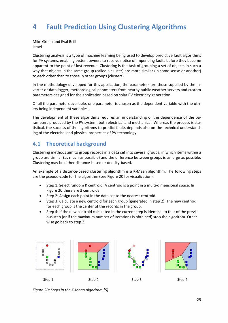
An example of a distance-based clustering algorithm is a K-Mean algorithm. The following steps are the pseudo-code for the algorithm (see Figure 20 for visualization).

Step 1: Select random K centroid. A centroid is a point in a multi-dimensional space. In Figure 20 there are 3 centroids

Step 2: Assign each point in the data set to the nearest centroid.

Step 3: Calculate a new centroid for each group (generated in step 2). The new centroid for each group is the center of the records in the group.

Step 4: If the new centroid calculated in the current step is identical to that of the previ-ous step (or if the maximum number of iterations is obtained) stop the algorithm. Other-wise go back to step 2.

Figure 20: Steps in the K-Mean algorithm [5]

30

The advantage of this algorithm is its simplicity and relatively short time for converging to a solu-tion. The disadvantage of this algorithm is its inability to discover the optimal number of clusters automatically.

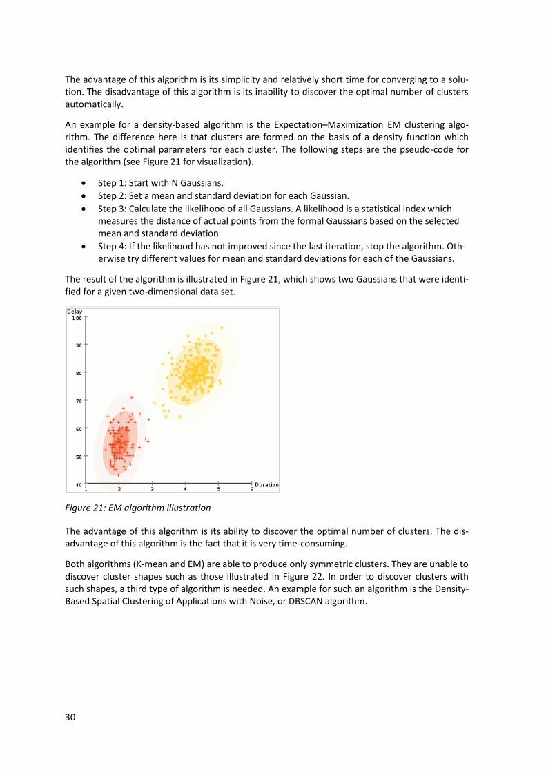
An example for a density-based algorithm is the Expectation–Maximization EM clustering algo-rithm. The difference here is that clusters are formed on the basis of a density function which identifies the optimal parameters for each cluster. The following steps are the pseudo-code for the algorithm (see Figure 21 for visualization).

Step 1: Start with N Gaussians.

Step 2: Set a mean and standard deviation for each Gaussian.

Step 3: Calculate the likelihood of all Gaussians. A likelihood is a statistical index which measures the distance of actual points from the formal Gaussians based on the selected mean and standard deviation.

Step 4: If the likelihood has not improved since the last iteration, stop the algorithm. Oth-erwise try different values for mean and standard deviations for each of the Gaussians.

The result of the algorithm is illustrated in Figure 21, which shows two Gaussians that were identi-fied for a given two-dimensional data set.

Figure 21: EM algorithm illustration

The advantage of this algorithm is its ability to discover the optimal number of clusters. The dis-advantage of this algorithm is the fact that it is very time-consuming.

Both algorithms (K-mean and EM) are able to produce only symmetric clusters. They are unable to discover cluster shapes such as those illustrated in Figure 22. In order to discover clusters with such shapes, a third type of algorithm is needed. An example for such an algorithm is the Density-Based Spatial Clustering of Applications with Noise, or DBSCAN algorithm.

31

Figure 22: Non-symmetric clusters

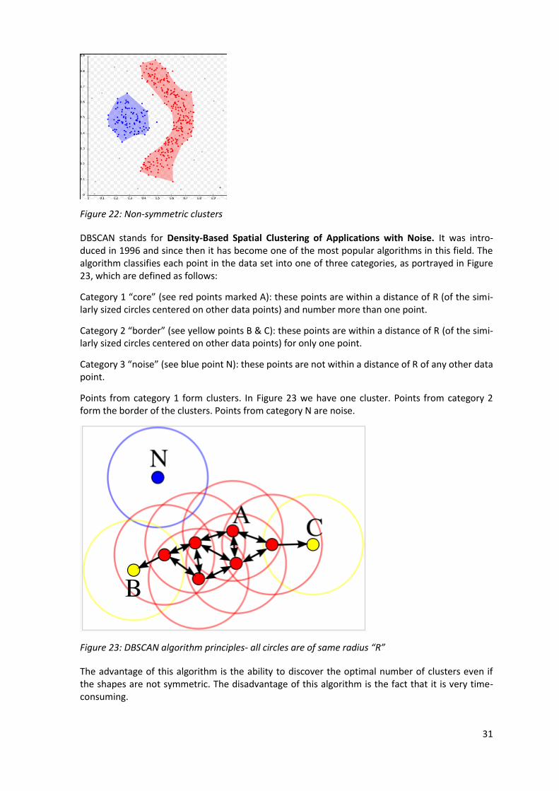
DBSCAN stands for Density-Based Spatial Clustering of Applications with Noise. It was intro-duced in 1996 and since then it has become one of the most popular algorithms in this field. The algorithm classifies each point in the data set into one of three categories, as portrayed in Figure 23, which are defined as follows:

Category 1 “core” (see red points marked A): these points are within a distance of R (of the simi-larly sized circles centered on other data points) and number more than one point.

Category 2 “border” (see yellow points B & C): these points are within a distance of R (of the simi-larly sized circles centered on other data points) for only one point.

Category 3 “noise” (see blue point N): these points are not within a distance of R of any other data point.

Points from category 1 form clusters. In Figure 23 we have one cluster. Points from category 2 form the border of the clusters. Points from category N are noise.

Figure 23: DBSCAN algorithm principles- all circles are of same radius “R”

The advantage of this algorithm is the ability to discover the optimal number of clusters even if the shapes are not symmetric. The disadvantage of this algorithm is the fact that it is very time-consuming.

32

4.2 Methodology

For the purpose of developing and testing the algorithms, the following methodology was defined for commencing the learning process.

The following steps have been defined for preparing and testing the clustering:

Step 1: Generate a clear data set (e.g. 4 months of 15-min data) of whatever inverter parameters are available from the inspected system and publicly accessible meteorological data (initial learn-ing process).

Step 2: Choose the output value as a dependent (examined) parameter; at this point of develop-ment we are using AC power (generation) as the dependent parameter, since a drop in power is a fault causing financial loss.

Step 3: Add the following to each record:

Electricity generation for the previous hour Electricity generation for the same hour a day before Day of the year expressed as sin(day), cos(day) transformation

)365

2cos(),

365

2sin(

dayofyeardayofyear

Step 4: For each cluster, an equation is developed that defines the relationship between all the independent values and the single dependent value. Each internal equation is devised to ensure a Confidence Interval [CI] of 99 %. The Confidence Interval is calculated using either a parametric (normal distribution) or non-parametric method.

Step 5: Run a new set of data through the clustering equations and check the equation output versus the real dependent values for the examined variable - the real values should fall within the Confidence Interval of 0.001 (probability).

Step 6: All new data running through the equations should now fall within the Confidence Interval of the predicted values from the clustering; if not, we may have an impending fault

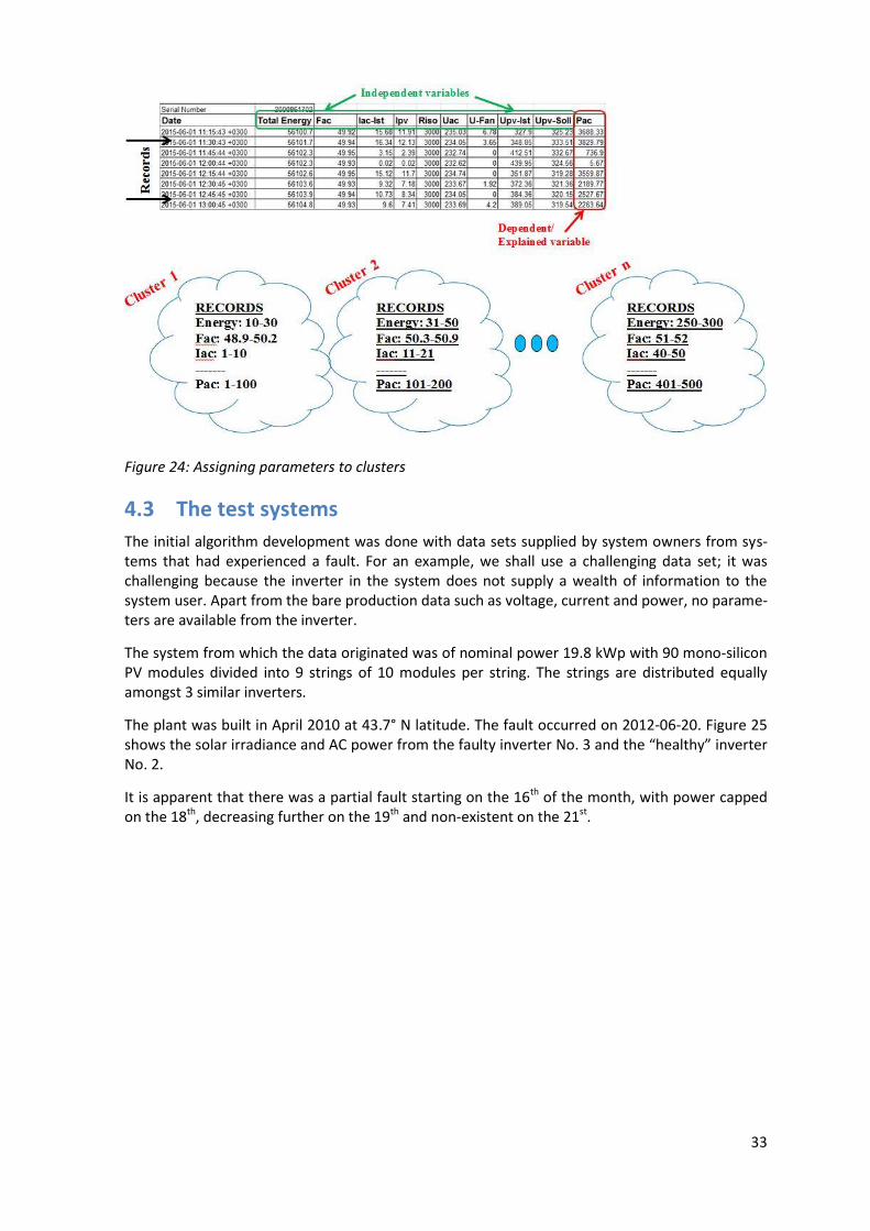
Figure 24 portrays the thought behind choosing the clusters. The generated power parameter (Pac) is chosen as the dependent value, since this value is the end result of the purpose to gener-ate electricity. This is the parameter that is failing from the authors’ point of view.

The remaining parameters are independent variables. The clusters are chosen by clustering the data set with methods as described in the previous section.

33

Figure 24: Assigning parameters to clusters

4.3 The test systems

The initial algorithm development was done with data sets supplied by system owners from sys-tems that had experienced a fault. For an example, we shall use a challenging data set; it was challenging because the inverter in the system does not supply a wealth of information to the system user. Apart from the bare production data such as voltage, current and power, no parame-ters are available from the inverter.

The system from which the data originated was of nominal power 19.8 kWp with 90 mono-silicon PV modules divided into 9 strings of 10 modules per string. The strings are distributed equally amongst 3 similar inverters.

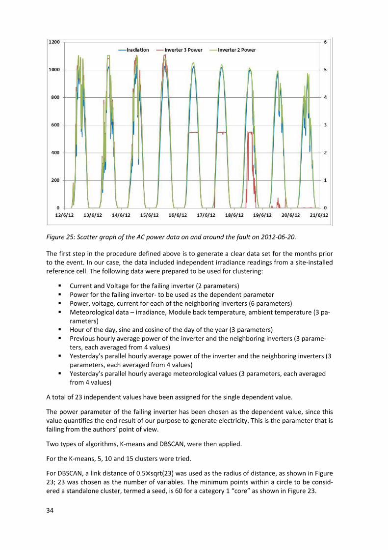
The plant was built in April 2010 at 43.7° N latitude. The fault occurred on 2012-06-20. Figure 25 shows the solar irradiance and AC power from the faulty inverter No. 3 and the “healthy” inverter No. 2.

It is apparent that there was a partial fault starting on the 16th of the month, with power capped on the 18th, decreasing further on the 19th and non-existent on the 21st.

34

Figure 25: Scatter graph of the AC power data on and around the fault on 2012-06-20.

The first step in the procedure defined above is to generate a clear data set for the months prior to the event. In our case, the data included independent irradiance readings from a site-installed reference cell. The following data were prepared to be used for clustering:

Current and Voltage for the failing inverter (2 parameters) Power for the failing inverter- to be used as the dependent parameter Power, voltage, current for each of the neighboring inverters (6 parameters) Meteorological data – irradiance, Module back temperature, ambient temperature (3 pa-

rameters) Hour of the day, sine and cosine of the day of the year (3 parameters) Previous hourly average power of the inverter and the neighboring inverters (3 parame-

ters, each averaged from 4 values) Yesterday’s parallel hourly average power of the inverter and the neighboring inverters (3

parameters, each averaged from 4 values) Yesterday’s parallel hourly average meteorological values (3 parameters, each averaged

from 4 values)

A total of 23 independent values have been assigned for the single dependent value.

The power parameter of the failing inverter has been chosen as the dependent value, since this value quantifies the end result of our purpose to generate electricity. This is the parameter that is failing from the authors’ point of view.

Two types of algorithms, K-means and DBSCAN, were then applied.

For the K-means, 5, 10 and 15 clusters were tried.

For DBSCAN, a link distance of 0.5×sqrt(23) was used as the radius of distance, as shown in Figure 23; 23 was chosen as the number of variables. The minimum points within a circle to be consid-ered a standalone cluster, termed a seed, is 60 for a category 1 “core” as shown in Figure 23.

35

4.4 Results

We ran the data set using different numbers of clusters in K-mean and found that there was no difference in the outcome between the sets using 5 clusters or more than 5 clusters.

We ran both the K-mean and DBSCAN using both a parametric and non-parametric confidence interval.

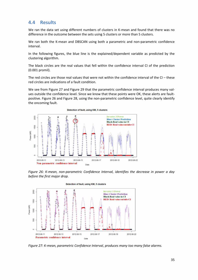
In the following figures, the blue line is the explained/dependent variable as predicted by the clustering algorithm.

The black circles are the real values that fell within the confidence interval CI of the prediction (0.001 promil).

The red circles are those real values that were not within the confidence interval of the CI – these red circles are indications of a fault condition.

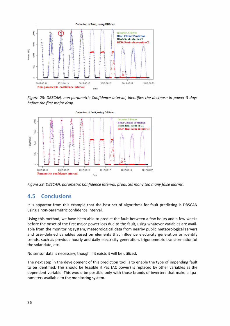
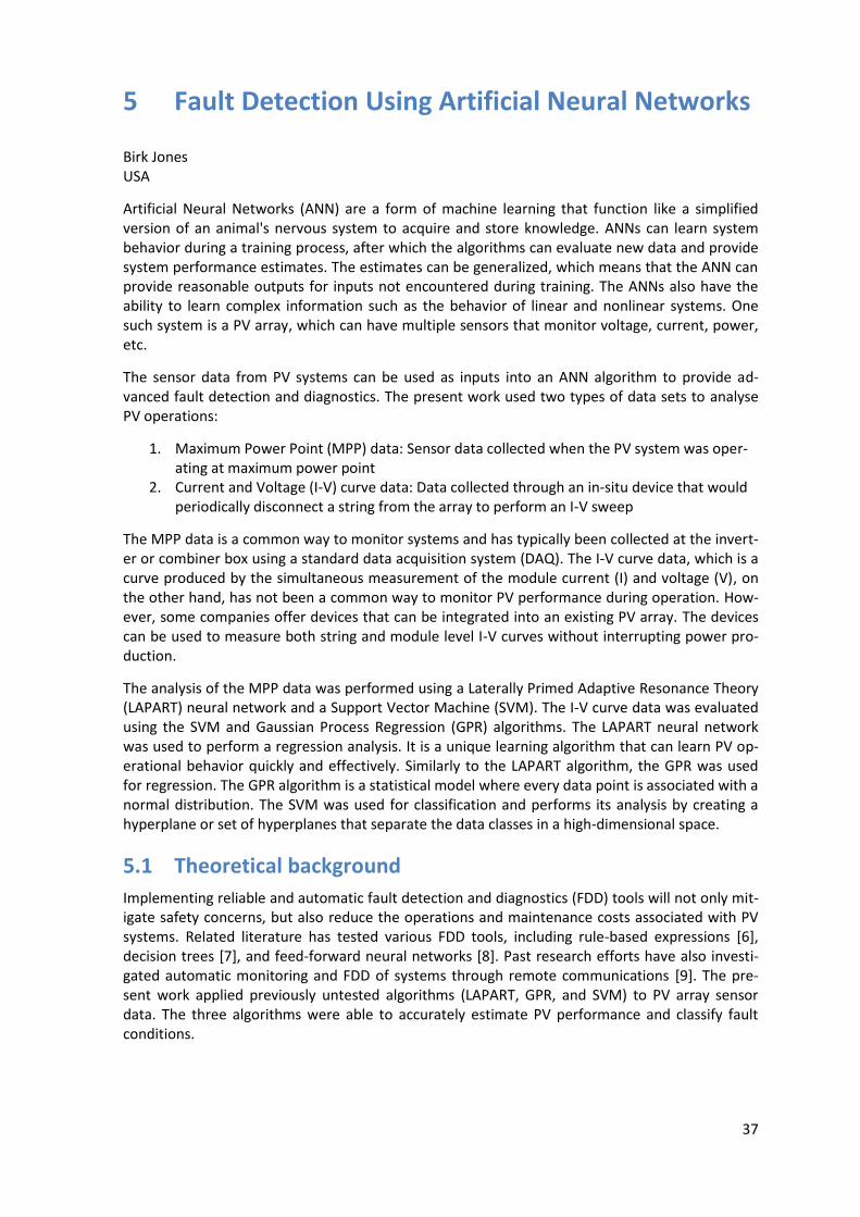
We see from Figure 27 and Figure 29 that the parametric confidence interval produces many val-ues outside the confidence level. Since we know that these points were OK, these alerts are fault-positive. Figure 26 and Figure 28, using the non-parametric confidence level, quite clearly identify the oncoming fault.

Figure 26: K-mean, non-parametric Confidence Interval, identifies the decrease in power a day before the first major drop.

Figure 27: K-mean, parametric Confidence Interval, produces many too many false alarms.

36

Figure 28: DBSCAN, non-parametric Confidence Interval, identifies the decrease in power 3 days before the first major drop.

Figure 29: DBSCAN, parametric Confidence Interval, produces many too many false alarms.

4.5 Conclusions

It is apparent from this example that the best set of algorithms for fault predicting is DBSCAN using a non-parametric confidence interval.

Using this method, we have been able to predict the fault between a few hours and a few weeks before the onset of the first major power loss due to the fault, using whatever variables are avail-able from the monitoring system, meteorological data from nearby public meteorological servers and user-defined variables based on elements that influence electricity generation or identify trends, such as previous hourly and daily electricity generation, trigonometric transformation of the solar date, etc.

No sensor data is necessary, though if it exists it will be utilized.

The next step in the development of this prediction tool is to enable the type of impending fault to be identified. This should be feasible if Pac (AC power) is replaced by other variables as the dependent variable. This would be possible only with those brands of inverters that make all pa-rameters available to the monitoring system.

37

5 Fault Detection Using Artificial Neural Networks

Birk Jones USA

Artificial Neural Networks (ANN) are a form of machine learning that function like a simplified version of an animal's nervous system to acquire and store knowledge. ANNs can learn system behavior during a training process, after which the algorithms can evaluate new data and provide system performance estimates. The estimates can be generalized, which means that the ANN can provide reasonable outputs for inputs not encountered during training. The ANNs also have the ability to learn complex information such as the behavior of linear and nonlinear systems. One such system is a PV array, which can have multiple sensors that monitor voltage, current, power, etc.

The sensor data from PV systems can be used as inputs into an ANN algorithm to provide ad-vanced fault detection and diagnostics. The present work used two types of data sets to analyse PV operations:

1. Maximum Power Point (MPP) data: Sensor data collected when the PV system was oper-ating at maximum power point

2. Current and Voltage (I-V) curve data: Data collected through an in-situ device that would periodically disconnect a string from the array to perform an I-V sweep

The MPP data is a common way to monitor systems and has typically been collected at the invert-er or combiner box using a standard data acquisition system (DAQ). The I-V curve data, which is a curve produced by the simultaneous measurement of the module current (I) and voltage (V), on the other hand, has not been a common way to monitor PV performance during operation. How-ever, some companies offer devices that can be integrated into an existing PV array. The devices can be used to measure both string and module level I-V curves without interrupting power pro-duction.

The analysis of the MPP data was performed using a Laterally Primed Adaptive Resonance Theory (LAPART) neural network and a Support Vector Machine (SVM). The I-V curve data was evaluated using the SVM and Gaussian Process Regression (GPR) algorithms. The LAPART neural network was used to perform a regression analysis. It is a unique learning algorithm that can learn PV op-erational behavior quickly and effectively. Similarly to the LAPART algorithm, the GPR was used for regression. The GPR algorithm is a statistical model where every data point is associated with a normal distribution. The SVM was used for classification and performs its analysis by creating a hyperplane or set of hyperplanes that separate the data classes in a high-dimensional space.

5.1 Theoretical background

Implementing reliable and automatic fault detection and diagnostics (FDD) tools will not only mit-igate safety concerns, but also reduce the operations and maintenance costs associated with PV systems. Related literature has tested various FDD tools, including rule-based expressions [6], decision trees [7], and feed-forward neural networks [8]. Past research efforts have also investi-gated automatic monitoring and FDD of systems through remote communications [9]. The pre-sent work applied previously untested algorithms (LAPART, GPR, and SVM) to PV array sensor data. The three algorithms were able to accurately estimate PV performance and classify fault conditions.

38

5.1.1 Laterally Primed Adaptive Resonance Theory (LAPART)

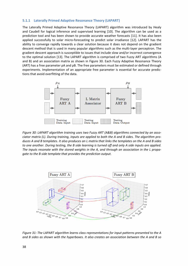
The Laterally Primed Adaptive Resonance Theory (LAPART) algorithm was introduced by Healy and Caudell for logical inference and supervised learning [10]. The algorithm can be used as a prediction tool and has been shown to provide accurate weather forecasts [11]. It has also been applied successfully to solar micro-forecasting to predict solar irradiance [12]. LAPART has the ability to converge rapidly towards a clear solution because it does not depend on the gradient descent method that is used in many popular algorithms such as the multi-layer perceptron. The gradient descent approach is susceptible to issues that include slow and/or incorrect convergence to the optimal solution [13]. The LAPART algorithm is comprised of two Fuzzy ART algorithms (A and B) and an association matrix as shown in Figure 30. Each Fuzzy Adaptive Resonance Theory (ART) has a free parameter ρA and ρB. The free parameters must be estimated or defined through experiments. Implementation of an appropriate free parameter is essential for accurate predic-tions that avoid overfitting of the data.

Figure 30: LAPART algorithm training uses two Fuzzy ART (A&B) algorithms connected by an asso-ciator matrix (L). During training, inputs are applied to both the A and B sides. The algorithm pro-duces A and B templates. It also produces an L matrix that links the templates on the A and B sides to one another. During testing, the B side learning is turned off and only A side inputs are applied. The inputs resonate with the stored weights in the A, and through an association in the L propa-gate to the B side template that provides the prediction output.

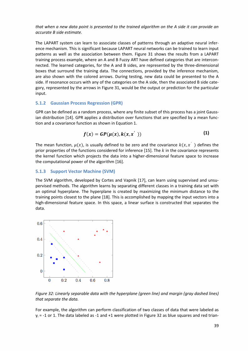
Figure 31: The LAPART algorithm learns class representations for input patterns presented to the A and B sides as shown with the hyperboxes. It also creates an association between the A and B so

39

that when a new data point is presented to the trained algorithm on the A side it can provide an accurate B side estimate.

The LAPART system can learn to associate classes of patterns through an adaptive neural infer-ence mechanism. This is significant because LAPART neural networks can be trained to learn input patterns as well as the association between them. Figure 31 shows the results from a LAPART training process example, where an A and B Fuzzy ART have defined categories that are intercon-nected. The learned categories, for the A and B sides, are represented by the three-dimensional boxes that surround the training data. The connections, provided by the inference mechanism, are also shown with the colored arrows. During testing, new data could be presented to the A side. If resonance occurs with any of the categories on the A side, then the associated B side cate-gory, represented by the arrows in Figure 31, would be the output or prediction for the particular input.

5.1.2 Gaussian Process Regression (GPR)

GPR can be defined as a random process, where any finite subset of this process has a joint Gauss-ian distribution [14]. GPR applies a distribution over functions that are specified by a mean func-tion and a covariance function as shown in Equation 1.

𝒇(𝒙) = 𝑮𝑷(𝝁(𝒙), 𝒌(𝒙, 𝒙′)) (1)

The mean function, 𝜇(𝑥), is usually defined to be zero and the covariance 𝑘(𝑥, 𝑥′) defines the prior properties of the functions considered for inference [15]. The 𝑘 in the covariance represents the kernel function which projects the data into a higher-dimensional feature space to increase the computational power of the algorithm [16].

5.1.3 Support Vector Machine (SVM)

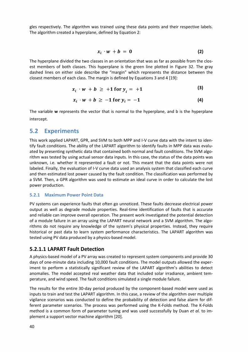
The SVM algorithm, developed by Cortes and Vapnik [17], can learn using supervised and unsu-pervised methods. The algorithm learns by separating different classes in a training data set with an optimal hyperplane. The hyperplane is created by maximizing the minimum distance to the training points closest to the plane [18]. This is accomplished by mapping the input vectors into a high-dimensional feature space. In this space, a linear surface is constructed that separates the data.

Figure 32: Linearly separable data with the hyperplane (green line) and margin (gray dashed lines) that separate the data.

For example, the algorithm can perform classification of two classes of data that were labeled as yi = -1 or 1. The data labeled as -1 and +1 were plotted in Figure 32 as blue squares and red trian-

40

gles respectively. The algorithm was trained using these data points and their respective labels. The algorithm created a hyperplane, defined by Equation 2:

𝒙𝒊 ∙ 𝒘 + 𝒃 = 𝟎 (2)

The hyperplane divided the two classes in an orientation that was as far as possible from the clos-est members of both classes. This hyperplane is the green line plotted in Figure 32. The gray dashed lines on either side describe the “margin” which represents the distance between the closest members of each class. The margin is defined by Equations 3 and 4 [19]:

𝒙𝒊 ∙ 𝒘 + 𝒃 ≥ +𝟏 𝐟𝐨𝐫 𝒚𝒊

= +𝟏 (3)

𝒙𝒊 ⋅ 𝒘 + 𝒃 ≥ −𝟏 𝐟𝐨𝐫 𝒚𝒊 = −𝟏 (4)

The variable w represents the vector that is normal to the hyperplane, and b is the hyperplane

intercept.

5.2 Experiments

This work applied LAPART, GPR, and SVM to both MPP and I-V curve data with the intent to iden-tify fault conditions. The ability of the LAPART algorithm to identify faults in MPP data was evalu-ated by presenting synthetic data that contained both normal and fault conditions. The SVM algo-rithm was tested by using actual sensor data inputs. In this case, the status of the data points was unknown, i.e. whether it represented a fault or not. This meant that the data points were not labeled. Finally, the evaluation of I-V curve data used an analysis system that classified each curve and then estimated lost power caused by the fault condition. The classification was performed by a SVM. Then, a GPR algorithm was used to estimate an ideal curve in order to calculate the lost power production.

5.2.1 Maximum Power Point Data

PV systems can experience faults that often go unnoticed. These faults decrease electrical power output as well as degrade module properties. Real-time identification of faults that is accurate and reliable can improve overall operation. The present work investigated the potential detection of a module failure in an array using the LAPART neural network and a SVM algorithm. The algo-rithms do not require any knowledge of the system’s physical properties. Instead, they require historical or past data to learn system performance characteristics. The LAPART algorithm was tested using PV data produced by a physics-based model.

5.2.1.1 LAPART Fault Detection A physics-based model of a PV array was created to represent system components and provide 30 days of one-minute data including 10,000 fault conditions. The model outputs allowed the exper-iment to perform a statistically significant review of the LAPART algorithm’s abilities to detect anomalies. The model accepted real weather data that included solar irradiance, ambient tem-perature, and wind speed. The fault conditions simulated a single module failure.

The results for the entire 30-day period produced by the component-based model were used as inputs to train and test the LAPART algorithm. In this case, a review of the algorithm over multiple vigilance scenarios was conducted to define the probability of detection and false alarm for dif-ferent parameter scenarios. The process was performed using the K-Folds method. The K-Folds method is a common form of parameter tuning and was used successfully by Duan et al. to im-plement a support vector machine algorithm [20].

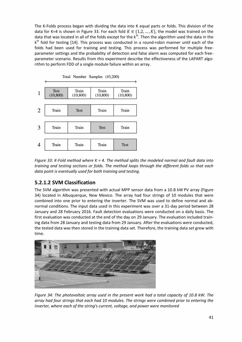
41

The K-Folds process began with dividing the data into K equal parts or folds. This division of the data for K=4 is shown in Figure 33. For each fold 𝐾 ∈ {1,2, … , 𝐾}, the model was trained on the data that was located in all of the folds except for the kth. Then the algorithm used the data in the kth fold for testing [14]. This process was conducted in a round-robin manner until each of the folds had been used for training and testing. This process was performed for multiple free-parameter settings and the probability of detection and false alarm was computed for each free-parameter scenario. Results from this experiment describe the effectiveness of the LAPART algo-rithm to perform FDD of a single module failure within an array.

Figure 33: K-Fold method where K = 4. The method splits the modeled normal and fault data into training and testing sections or folds. The method loops through the different folds so that each data point is eventually used for both training and testing.

5.2.1.2 SVM Classification The SVM algorithm was presented with actual MPP sensor data from a 10.8 kW PV array (Figure 34) located in Albuquerque, New Mexico. The array had four strings of 10 modules that were combined into one prior to entering the inverter. The SVM was used to define normal and ab-normal conditions. The input data used in this experiment was over a 31-day period between 28 January and 28 February 2016. Fault detection evaluations were conducted on a daily basis. The first evaluation was conducted at the end of the day on 29 January. The evaluation included train-ing data from 28 January and testing data from 29 January. After the evaluations were conducted, the tested data was then stored in the training data set. Therefore, the training data set grew with time.

Figure 34: The photovoltaic array used in the present work had a total capacity of 10.8 kW. The array had four strings that each had 10 modules. The strings were combined prior to entering the inverter, where each of the string's current, voltage, and power were monitored

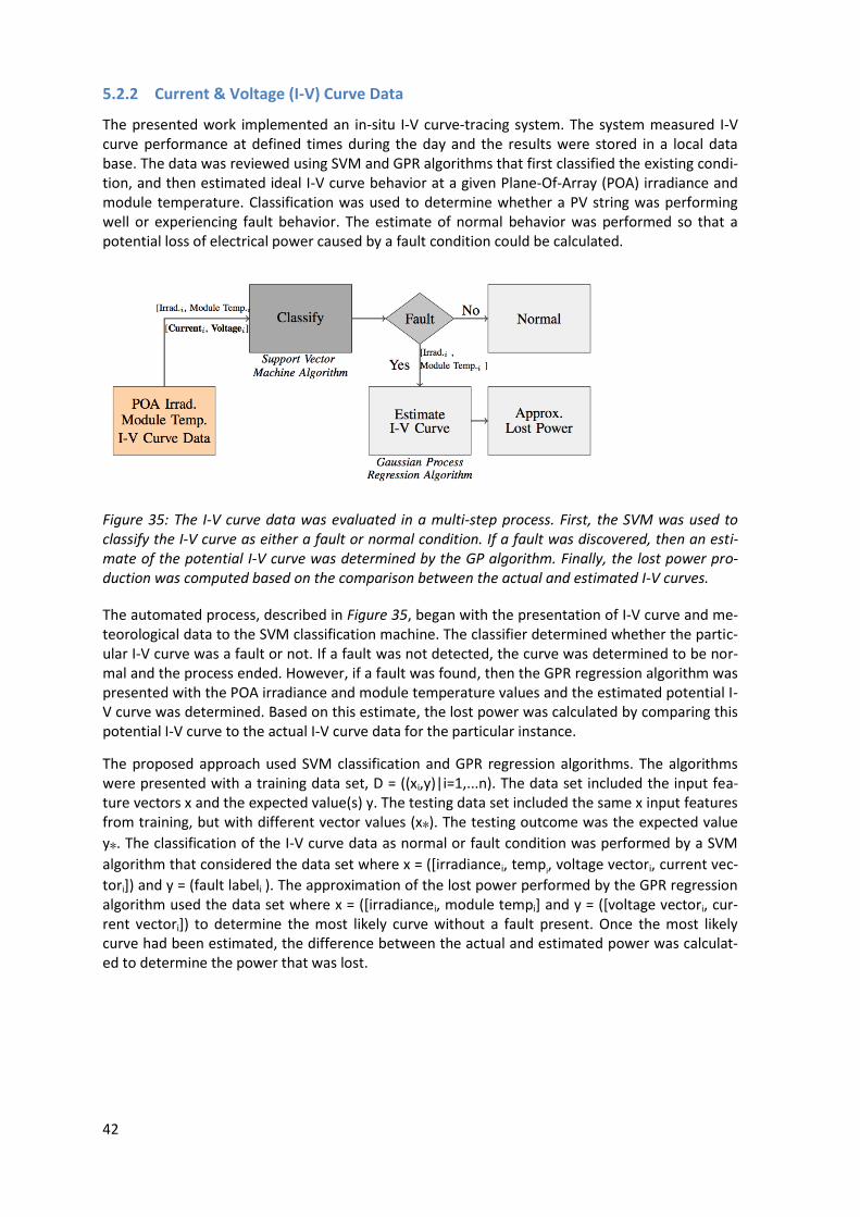
42

5.2.2 Current & Voltage (I-V) Curve Data

The presented work implemented an in-situ I-V curve-tracing system. The system measured I-V curve performance at defined times during the day and the results were stored in a local data base. The data was reviewed using SVM and GPR algorithms that first classified the existing condi-tion, and then estimated ideal I-V curve behavior at a given Plane-Of-Array (POA) irradiance and module temperature. Classification was used to determine whether a PV string was performing well or experiencing fault behavior. The estimate of normal behavior was performed so that a potential loss of electrical power caused by a fault condition could be calculated.

Figure 35: The I-V curve data was evaluated in a multi-step process. First, the SVM was used to classify the I-V curve as either a fault or normal condition. If a fault was discovered, then an esti-mate of the potential I-V curve was determined by the GP algorithm. Finally, the lost power pro-duction was computed based on the comparison between the actual and estimated I-V curves.

The automated process, described in Figure 35, began with the presentation of I-V curve and me-teorological data to the SVM classification machine. The classifier determined whether the partic-ular I-V curve was a fault or not. If a fault was not detected, the curve was determined to be nor-mal and the process ended. However, if a fault was found, then the GPR regression algorithm was presented with the POA irradiance and module temperature values and the estimated potential I-V curve was determined. Based on this estimate, the lost power was calculated by comparing this potential I-V curve to the actual I-V curve data for the particular instance.

The proposed approach used SVM classification and GPR regression algorithms. The algorithms were presented with a training data set, D = ((xi,y)|i=1,...n). The data set included the input fea-ture vectors x and the expected value(s) y. The testing data set included the same x input features from training, but with different vector values (x∗). The testing outcome was the expected value

y∗. The classification of the I-V curve data as normal or fault condition was performed by a SVM

algorithm that considered the data set where x = ([irradiancei, tempi, voltage vectori, current vec-

tori]) and y = (fault labeli ). The approximation of the lost power performed by the GPR regression algorithm used the data set where x = ([irradiancei, module tempi] and y = ([voltage vectori, cur-rent vectori]) to determine the most likely curve without a fault present. Once the most likely curve had been estimated, the difference between the actual and estimated power was calculat-ed to determine the power that was lost.

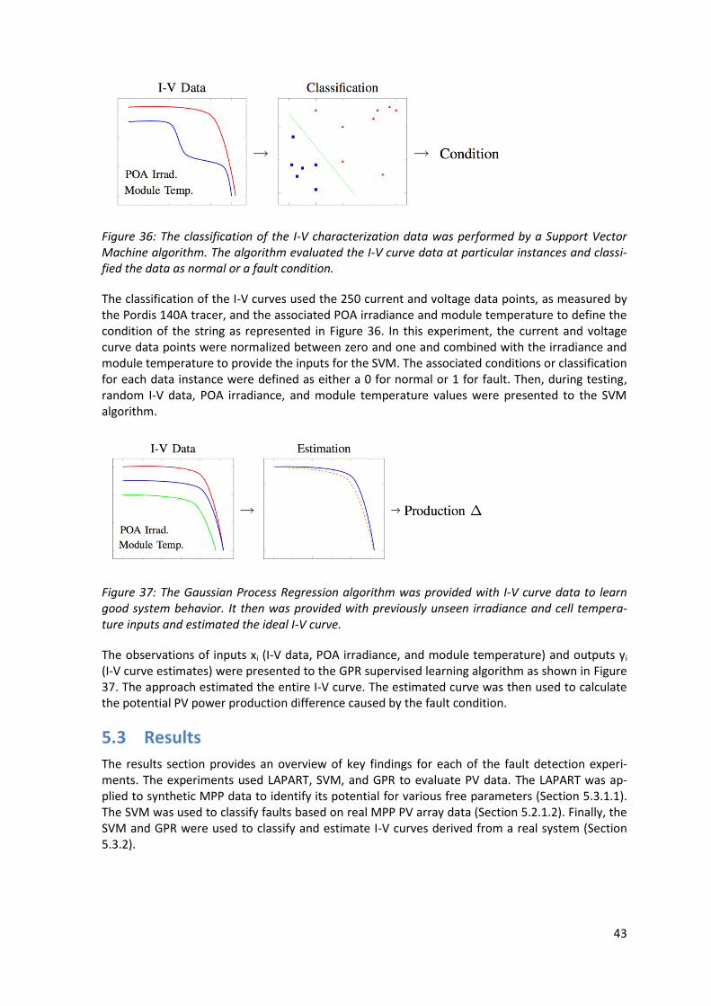
43

Figure 36: The classification of the I-V characterization data was performed by a Support Vector Machine algorithm. The algorithm evaluated the I-V curve data at particular instances and classi-fied the data as normal or a fault condition.

The classification of the I-V curves used the 250 current and voltage data points, as measured by the Pordis 140A tracer, and the associated POA irradiance and module temperature to define the condition of the string as represented in Figure 36. In this experiment, the current and voltage curve data points were normalized between zero and one and combined with the irradiance and module temperature to provide the inputs for the SVM. The associated conditions or classification for each data instance were defined as either a 0 for normal or 1 for fault. Then, during testing, random I-V data, POA irradiance, and module temperature values were presented to the SVM algorithm.

Figure 37: The Gaussian Process Regression algorithm was provided with I-V curve data to learn good system behavior. It then was provided with previously unseen irradiance and cell tempera-ture inputs and estimated the ideal I-V curve.

The observations of inputs xi (I-V data, POA irradiance, and module temperature) and outputs yi (I-V curve estimates) were presented to the GPR supervised learning algorithm as shown in Figure 37. The approach estimated the entire I-V curve. The estimated curve was then used to calculate the potential PV power production difference caused by the fault condition.

5.3 Results

The results section provides an overview of key findings for each of the fault detection experi-ments. The experiments used LAPART, SVM, and GPR to evaluate PV data. The LAPART was ap-plied to synthetic MPP data to identify its potential for various free parameters (Section 5.3.1.1). The SVM was used to classify faults based on real MPP PV array data (Section 5.2.1.2). Finally, the SVM and GPR were used to classify and estimate I-V curves derived from a real system (Section 5.3.2).

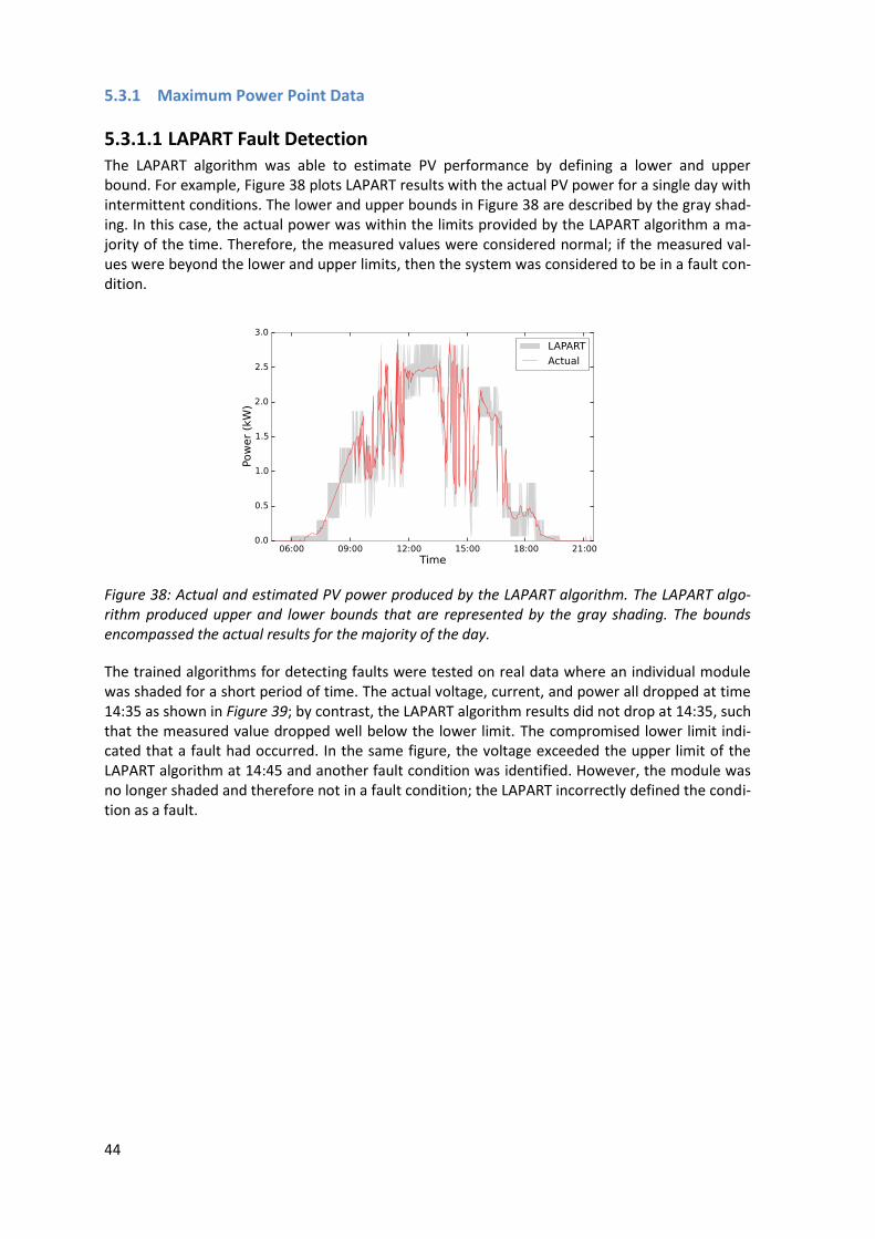
44

5.3.1 Maximum Power Point Data

5.3.1.1 LAPART Fault Detection The LAPART algorithm was able to estimate PV performance by defining a lower and upper bound. For example, Figure 38 plots LAPART results with the actual PV power for a single day with intermittent conditions. The lower and upper bounds in Figure 38 are described by the gray shad-ing. In this case, the actual power was within the limits provided by the LAPART algorithm a ma-jority of the time. Therefore, the measured values were considered normal; if the measured val-ues were beyond the lower and upper limits, then the system was considered to be in a fault con-dition.

Figure 38: Actual and estimated PV power produced by the LAPART algorithm. The LAPART algo-rithm produced upper and lower bounds that are represented by the gray shading. The bounds encompassed the actual results for the majority of the day.

The trained algorithms for detecting faults were tested on real data where an individual module was shaded for a short period of time. The actual voltage, current, and power all dropped at time 14:35 as shown in Figure 39; by contrast, the LAPART algorithm results did not drop at 14:35, such that the measured value dropped well below the lower limit. The compromised lower limit indi-cated that a fault had occurred. In the same figure, the voltage exceeded the upper limit of the LAPART algorithm at 14:45 and another fault condition was identified. However, the module was no longer shaded and therefore not in a fault condition; the LAPART incorrectly defined the condi-tion as a fault.

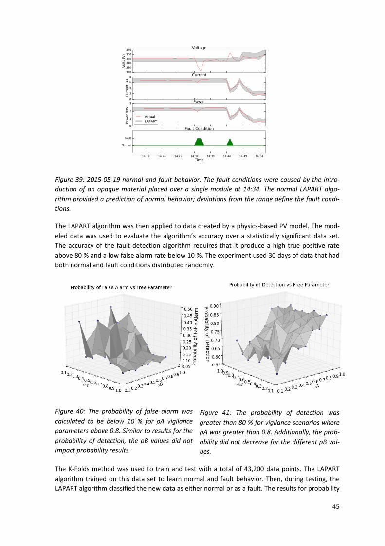
45

Figure 39: 2015-05-19 normal and fault behavior. The fault conditions were caused by the intro-

duction of an opaque material placed over a single module at 14:34. The normal LAPART algo-

rithm provided a prediction of normal behavior; deviations from the range define the fault condi-

tions.

The LAPART algorithm was then applied to data created by a physics-based PV model. The mod-

eled data was used to evaluate the algorithm’s accuracy over a statistically significant data set.

The accuracy of the fault detection algorithm requires that it produce a high true positive rate

above 80 % and a low false alarm rate below 10 %. The experiment used 30 days of data that had

both normal and fault conditions distributed randomly.

Figure 40: The probability of false alarm was

calculated to be below 10 % for ρA vigilance

parameters above 0.8. Similar to results for the

probability of detection, the ρB values did not

impact probability results.

Figure 41: The probability of detection was

greater than 80 % for vigilance scenarios where

ρA was greater than 0.8. Additionally, the prob-

ability did not decrease for the different ρB val-

ues.

The K-Folds method was used to train and test with a total of 43,200 data points. The LAPART

algorithm trained on this data set to learn normal and fault behavior. Then, during testing, the

LAPART algorithm classified the new data as either normal or as a fault. The results for probability

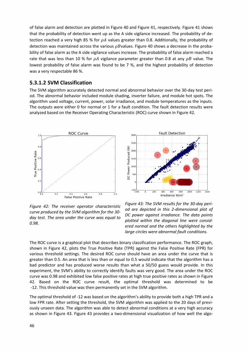
46

of false alarm and detection are plotted in Figure 40 and Figure 41, respectively. Figure 41 shows

that the probability of detection went up as the A side vigilance increased. The probability of de-

tection reached a very high 85 % for 𝜌𝐴 values greater than 0.8. Additionally, the probability of

detection was maintained across the various 𝜌𝐵values. Figure 40 shows a decrease in the proba-

bility of false alarm as the A side vigilance values increase. The probability of false alarm reached a

rate that was less than 10 % for 𝜌𝐴 vigilance parameter greater than 0.8 at any 𝜌𝐵 value. The

lowest probability of false alarm was found to be 7 %, and the highest probability of detection

was a very respectable 86 %.

5.3.1.2 SVM Classification The SVM algorithm accurately detected normal and abnormal behavior over the 30-day test peri-od. The abnormal behavior included module shading, inverter failure, and module hot spots. The algorithm used voltage, current, power, solar irradiance, and module temperatures as the inputs. The outputs were either 0 for normal or 1 for a fault condition. The fault detection results were analyzed based on the Receiver Operating Characteristic (ROC) curve shown in Figure 42.

Figure 42: The receiver operator characteristic curve produced by the SVM algorithm for the 30-day test. The area under the curve was equal to 0.98.

Figure 43: The SVM results for the 30-day peri-od are depicted in this 2-dimensional plot of DC power against irradiance. The data points plotted within the diagonal line were consid-ered normal and the others highlighted by the large circles were abnormal fault conditions.

The ROC curve is a graphical plot that describes binary classification performance. The ROC graph, shown in Figure 42, plots the True Positive Rate (TPR) against the False Positive Rate (FPR) for various threshold settings. The desired ROC curve should have an area under the curve that is greater than 0.5. An area that is less than or equal to 0.5 would indicate that the algorithm has a bad predictor and has produced worse results than what a 50/50 guess would provide. In this experiment, the SVM’s ability to correctly identify faults was very good. The area under the ROC curve was 0.98 and exhibited low false positive rates at high true positive rates as shown in Figure 42. Based on the ROC curve result, the optimal threshold was determined to be -12. This threshold value was then permanently set in the SVM algorithm.

The optimal threshold of -12 was based on the algorithm’s ability to provide both a high TPR and a low FPR rate. After setting the threshold, the SVM algorithm was applied to the 20 days of previ-ously unseen data. The algorithm was able to detect abnormal conditions at a very high accuracy as shown in Figure 43. Figure 43 provides a two-dimensional visualization of how well the algo-

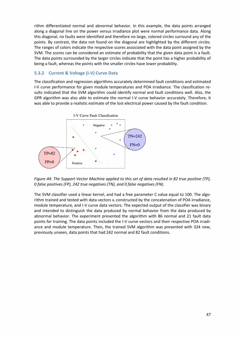
47

rithm differentiated normal and abnormal behavior. In this example, the data points arranged along a diagonal line on the power versus irradiance plot were normal performance data. Along this diagonal, no faults were identified and therefore no large, colored circles surround any of the points. By contrast, the data not found on the diagonal are highlighted by the different circles. The ranges of colors indicate the respective scores associated with the data point assigned by the SVM. The scores can be considered an estimate of probability that the given data point is a fault. The data points surrounded by the larger circles indicate that the point has a higher probability of being a fault, whereas the points with the smaller circles have lower probability.

5.3.2 Current & Voltage (I-V) Curve Data

The classification and regression algorithms accurately determined fault conditions and estimated I-V curve performance for given module temperatures and POA irradiance. The classification re-sults indicated that the SVM algorithm could identify normal and fault conditions well. Also, the GPR algorithm was also able to estimate the normal I-V curve behavior accurately. Therefore, it was able to provide a realistic estimate of the lost electrical power caused by the fault condition.

Figure 44: The Support Vector Machine applied to this set of data resulted in 82 true positive (TP), 0 false positives (FP), 242 true negatives (TN), and 0 false negatives (FN).

The SVM classifier used a linear kernel, and had a free parameter C value equal to 100. The algo-rithm trained and tested with data vectors xi constructed by the concatenation of POA irradiance, module temperature, and I-V curve data vectors. The expected output of the classifier was binary and intended to distinguish the data produced by normal behavior from the data produced by abnormal behavior. The experiment presented the algorithm with 86 normal and 21 fault data points for training. The data points included the I-V curve vectors and their respective POA irradi-ance and module temperature. Then, the trained SVM algorithm was presented with 324 new, previously unseen, data points that had 242 normal and 82 fault conditions.

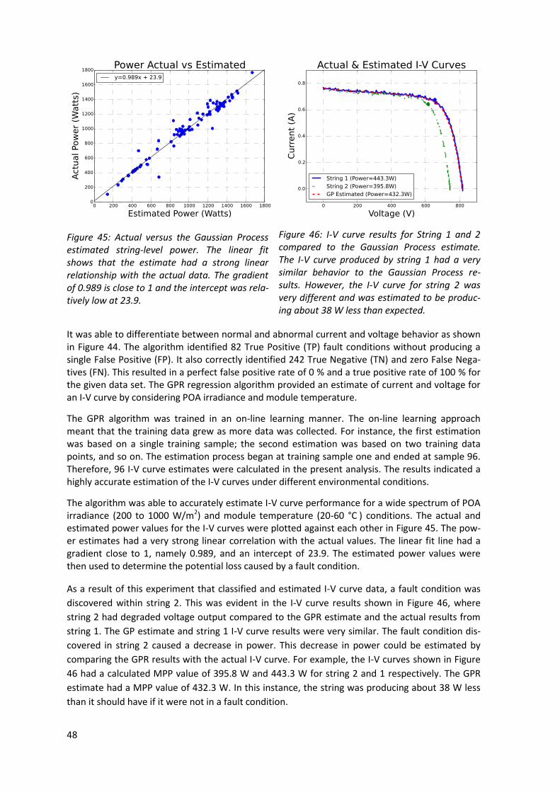
48

Figure 45: Actual versus the Gaussian Process estimated string-level power. The linear fit shows that the estimate had a strong linear relationship with the actual data. The gradient of 0.989 is close to 1 and the intercept was rela-tively low at 23.9.

Figure 46: I-V curve results for String 1 and 2 compared to the Gaussian Process estimate. The I-V curve produced by string 1 had a very similar behavior to the Gaussian Process re-sults. However, the I-V curve for string 2 was very different and was estimated to be produc-ing about 38 W less than expected.

It was able to differentiate between normal and abnormal current and voltage behavior as shown in Figure 44. The algorithm identified 82 True Positive (TP) fault conditions without producing a single False Positive (FP). It also correctly identified 242 True Negative (TN) and zero False Nega-tives (FN). This resulted in a perfect false positive rate of 0 % and a true positive rate of 100 % for the given data set. The GPR regression algorithm provided an estimate of current and voltage for an I-V curve by considering POA irradiance and module temperature.

The GPR algorithm was trained in an on-line learning manner. The on-line learning approach meant that the training data grew as more data was collected. For instance, the first estimation was based on a single training sample; the second estimation was based on two training data points, and so on. The estimation process began at training sample one and ended at sample 96. Therefore, 96 I-V curve estimates were calculated in the present analysis. The results indicated a highly accurate estimation of the I-V curves under different environmental conditions.

The algorithm was able to accurately estimate I-V curve performance for a wide spectrum of POA irradiance (200 to 1000 W/m2) and module temperature (20-60 °C ) conditions. The actual and estimated power values for the I-V curves were plotted against each other in Figure 45. The pow-er estimates had a very strong linear correlation with the actual values. The linear fit line had a gradient close to 1, namely 0.989, and an intercept of 23.9. The estimated power values were then used to determine the potential loss caused by a fault condition.

As a result of this experiment that classified and estimated I-V curve data, a fault condition was

discovered within string 2. This was evident in the I-V curve results shown in Figure 46, where

string 2 had degraded voltage output compared to the GPR estimate and the actual results from

string 1. The GP estimate and string 1 I-V curve results were very similar. The fault condition dis-

covered in string 2 caused a decrease in power. This decrease in power could be estimated by

comparing the GPR results with the actual I-V curve. For example, the I-V curves shown in Figure

46 had a calculated MPP value of 395.8 W and 443.3 W for string 2 and 1 respectively. The GPR

estimate had a MPP value of 432.3 W. In this instance, the string was producing about 38 W less

than it should have if it were not in a fault condition.

49

5.4 Conclusions

Current recommendations for PV system oversight suggest metrics such as performance ratio (PR), temperature-corrected PR [21], Energy Performance Index (EPI), the NREL System Advisor Model model, EPI Regression model, and Power Performance Index (PPI). The PR is a measure of the theoretical and actual energy output. The theoretical output can be based on manufacturer specifications and not actual system performance. This calculation can be used to estimate the efficiency of the array, but cannot provide a detailed diagnostic of plant conditions. Advanced algorithms, such as machine learning and neural networks, have the ability to learn the actual system operational behavior with great detail under various operating conditions. This advanced learning approach provides plant operators with a detailed tool for analysis that is simple to im-plement. Additionally, the learning algorithm results can provide more detail and precision than the common PR.

The present work applied three algorithms that can be used to perform a detailed analysis of MPP and I-V curve data. The algorithms were used to detect faults and also estimate performance. The LAPART algorithm estimated PV performance by producing lower and upper bounds; if the meas-ured data fell outside of the bounds, it was determined to be in a fault condition. This approach was tested on synthetic data and fault data was introduced randomly. The LAPART algorithm was able to identify fault conditions at a TPR rate above 80 % and a FPR below 10 %. The SVM algo-rithm analyzed actual MPP data from a 10.8 kW array and was able to differentiate between nor-mal and abnormal behavior well. The approach produced an area under the ROC that was very close to 1. Finally, the proposed methodology to classify and then estimate lost power based on I-V curve data was implemented successfully. The SVM algorithm identified normal and abnormal behavior without producing a single false alarm. The GPR estimate showed a high linear relation-ship with the measured data and is a viable option for estimating I-V curve performance. The three algorithms were tested on a small sampling of data collected in Albuquerque, New Mexico. Future work requires that the algorithms be applied to data at various seasons and locations. Al-so, more testing and development is required to detect a wider variety of fault conditions.

50

6 Conclusions

In this report, we have examined four methods for fault detection using statistics as opposed to comparing parameters to acceptable set-points. All these methods offer quicker and more accu-rate detection of yield-reducing fault conditions than the methods currently in use by most off-the-shelf monitoring systems producing efficiency matrices such as the Performance Ratio, when irradiation sensors are available, or compare production to an assumed performance index or to a neighboring system.

As well as being quicker and more accurate, they require fewer inputs than existing systems, ena-bling the small-system owner to maintain a high level of PV plant efficiency, as he is alerted earlier to lower than acceptable power production than is possible without such statistical analysis. Each of the methods discussed has advantages and disadvantages. At time of writing, the ANN and clustering methods have yet to be commercialized.

The statistical evaluation of monitored data discussed in chapter 2 quickly ascertains when a fault condition exists and enables trouble-shooting of the fault. The advantages of this system over the current state of monitoring technology is that no irradiance or weather sensors are required; monitoring with the high time resolution provides real-time data and analysis specific to the sys-tem and includes advanced algorithms for different types of losses. Faults are quickly detected and identified and the system owner is advised of the fault and a recommended action.

The current state of the art for monitoring of residential PV plants (if monitoring exists at all) of-ten creates a warning that is not specific enough to allow specific corrective action. Furthermore, no other analysis tools are able to provide detailed trouble-shooting of the fault.

The disadvantage of this system is that it relies on weather data for the daily simulation process, which is available free of charge in Australia, but not for the rest of the world. The system also requires input from the home owner about the system specifications, and the physical installation of a monitoring unit in the household electrical power-meter box.

Machine learning for fast fault recognition enables even the smallest residential system owner to ascertain that their system is not operating optimally. The advantages of this system are that the system owner has only to supply access to inverter data, and that when a fault is perceived, the identification is based specifically on the system itself, enabling the owner to act with confidence on the alarm issued by the system.

The disadvantages to the system are that it is limited by the accuracy of the data supplied by the inverter and if a PV system has underperformed from the start, the detection system will not identify the underperformance.

Another advantage to this system is that when electricity tariffs begin to reflect the true cost of distributed generation on the distribution grid, and utilities begin to require NDH from residential customers, this algorithm will already be available. The system owner can then turn around and offer the same service to the utility, but based on next day’s weather predictions instead of yes-terday’s history.

Fault predictions using clustering machine-learning algorithms offer the quickest fault detection to date – before a major power-reducing fault occurs. The advantages of the system are that faults are predicted before they have a large impact, requiring no sensors or expensive irradiation maps and no information on system configuration. The system works solely on whatever produc-tion parameters are available. All that is required is a data feed from the inverter and meteorolog-ical data extracted from a local public meteorological server.

51

Fault detection based on artificial neural networks offers fast fault detection. The advantages of this system are that the alarms issued are produced by statistical analysis based on parameters produced by the system itself, and occur in real time. This system offers fault detection far faster than current commercially available systems, but does not require any knowledge of the system configuration.

The disadvantages of the system as it is presented here are a complexity that may require local computing power and the use of irradiance readings requiring sensors that are not available in small residential applications.

It is apparent from the four systems described in this report from three research and develop-ment centers, which are independent of each other and situated equally across 17 time zones, each serving their perceived market, that the state of the art for monitoring PV systems is moving from a sensor-based system to one of statistical calculations performed on system production parameters. This development comes about due to the granular nature of PV electricity genera-tion in a national grid. The total PV electricity generated in a national grid is largely supplied by many small systems with small financial plans that cannot support high-efficiency monitoring on their own. Statistical analysis requires no hardware, so the cost of the monitoring is flexible.

As the world moves towards distributed generation with multi-directional power flow within dis-tribution grids, these statistical methods will become crucial to retain efficiency and predict the electricity yield.

52

References

[1] Achim Woyte et al., “Analytical Monitoring of Grid-connected Photovoltaic Systems - Good Practice for Monitoring and Performance Analysis”, IEA PVPS Report T13-03: 2014, Mar. 2014.

[2] Thomas Nordmann, Wilfried G.J.H.M. van Sark, Mike Green, “Analysis of Long-Term Perfor-mance of PV Systems - Different Data Resolution for Different Purposes”, IEA-PVPS Report T13-05:2014, Nov. 2014, Page 39

[3] Australian Photovoltaic Institute, http://pv-map.apvi.org.au/ (2017-01-18)

[4] Australian Photovoltaic Institute, http://pv-map.apvi.org.au/ (2017-01-18)

[5] https://en.wikipedia.org/wiki/K-means_clustering#Initialization_methods (2017-01-18)

[6] A. Chouder and S. Silvestre, “Automatic supervision and fault detection of PV systems based on power losses analysis,” Energy Convers. Manag., vol. 51, no. 10, pp. 1929–1937, Oct. 2010.

[7] Y. Zhao, L. Yang, B. Lehman, J.-F. de Palma, J. Mosesian, and R. Lyons, “Decision tree-based fault detection and classification in solar photovoltaic arrays,” in 2012 Twenty-Seventh Annu-al IEEE Applied Power Electronics Conference and Exposition (APEC), 2012, pp. 93–99.

[8] D. Riley and J. Johnson, “Photovoltaic prognostics and heath management using learning algorithms,” in 2012 38th IEEE Photovoltaic Specialists Conference (PVSC), 2012, pp. 001535–001539.

[9] A. Drews, A. C. de Keizer, H. G. Beyer, E. Lorenz, J. Betcke, W. G. J. H. M. van Sark, W. Heyden-reich, E. Wiemken, S. Stettler, P. Toggweiler, S. Bofinger, M. Schneider, G. Heilscher, and D. Heinemann, “Monitoring and remote failure detection of grid-connected PV systems based on satellite observations,” Sol. Energy, vol. 81, no. 4, pp. 548–564, Apr. 2007.

[10] M. J. Healy, T. P. Caudell, and S. D. G. Smith, “A neural architecture for pattern sequence verification through inferencing,” IEEE Trans. Neural Netw., vol. 4, no. 1, pp. 9–20, Jan. 1993.

[11] M. J. Healy and T. P. Caudell, “Acquiring rule sets as a product of learning in a logical neural architecture,” IEEE Trans. Neural Netw., vol. 8, no. 3, pp. 461–474, May 1997.

[12] A. Mammoli, A. Menicucci, T. Caudell, A. Ellis, S. Willard, and J. Simmins, “Low-cost solar micro-forecasts for PV smoothing,” in 2013 1st IEEE Conference on Technologies for Sustaina-bility (SusTech), 2013, pp. 238–243.

[13] S. Haykin, Neural Networks A Comprehensive Foundation, 2nd ed. Prentice-Hall, Inc., 1999.

[14] K. P. Murphy, Machine Learning: A Probabilistic Perspective. MIT Press, 2012.

[15] C. E. Rasmussen and C. K. I. Williams, Gaussian Processes for Machine Learning. University Press Group Limited, 2006.

[16] J. Shawe-Taylor and N. Cristianini, Kernel Methods for Pattern Analysis. Cambridge University Press, 2004.

[17] C. Cortes and V. Vapnik, “Support-vector networks,” Mach. Learn., vol. 20, no. 3, pp. 273–297, Sep. 1995.

[18] S. Marsland, “Novelty detection in learning systems,” Neural Comput. Surv., vol. 3, no. 2, pp. 157–195, 2003.

53

[19] C. J. C. Burges, “A Tutorial on Support Vector Machines for Pattern Recognition,” Data Min. Knowl. Discov., vol. 2, no. 2, pp. 1–32, 1998.

[20] K. Duan, S. S. Keerthi, and A. N. Poo, “Evaluation of simple performance measures for tuning SVM hyperparameters,” Neurocomputing, vol. 51, pp. 41–59, Apr. 2003.

[21] V. Sharma, A. Kumar, O. S. Sastry, and S. S. Chandel, “Performance assessment of different solar photovoltaic technologies under similar outdoor conditions,” Energy, vol. 58, pp. 511–518, Sep. 2013.

54

For further information about the IEA Photovoltaic Power Systems Programme and Task 13 publi-cations, please visit www.iea-pvps.org.